EvoTorch: Scalable Evolutionary Computation in Python

Abstract

Evolutionary computation is an important component within various fields such as artificial intelligence research, reinforcement learning, robotics, industrial automation and/or optimization, engineering design, etc. Considering the increasing computational demands and the dimensionalities of modern optimization problems, the requirement for scalable, re-usable, and practical evolutionary algorithm implementations has been growing. To address this requirement, we present EvoTorch: an evolutionary computation library designed to work with high-dimensional optimization problems, with GPU support and with high parallelization capabilities. EvoTorch is based on and seamlessly works with the PyTorch library, and therefore, allows the users to define their optimization problems using a well-known API.

About this document

This document is a technical report describing version 0.4.0 of the EvoTorch evolutionary computation library. As the library is updated, corresponding updates will be made to this technical report. Please refer to this section, which you will find at the top of any version of this technical report, to find the corresponding version of the EvoTorch library to which this report refers.

EvoTorch is publicly available at https://github.com/nnaisense/evotorch/.

All GPU-based experiments were run on an NVIDIA DGX-Station with 4 16GB Tesla V100 GPUs, 256 GB DDR4 memory and 20-core, 40-thread Intel Xeon E5-2698 v4 processor.

1 Introduction

To use the definition of Back and Schwefel [1996], evolutionary computation (EC) is “an area of computer science that uses ideas from biological evolution to solve computational problems”. EC has become a popular approach for optimization and reinforcement learning due in large part to its flexibility and generality: the same evolutionary search procedure can be used to solve a wide range of tasks from static traveling salesman problems to optimizing neural network control policies. All that’s required in this black box setting is a function computes the relative "fitness" of each candidate solution, i.e. no gradient information needed. A the same time, when useful domain knowledge is available, EC makes it easy to incorporate this through problem-specific operators for further efficiency.

In order to leverage the full potential of this powerful approach, parallelization is the key—just as it, resoundingly, has been in the field of deep learning where today the default approach is to train enormous neural network models on GPUs [Chellapilla et al., 2006; Ciresan et al., 2011; Krizhevsky et al., 2012] (see survey [Schmidhuber, 2015]) using frameworks such as TensorFlow, Theano, PyTorch, etc. [James Bergstra et al., 2010; Tokui et al., 2015; Abadi et al., 2016; Yuret, 2016; Innes, 2018; Frostig et al., 2018; Paszke et al., 2019].

Because evolutionary algorithms use a population of solution points that can be evaluated independently, they are naturally suited for and can significantly benefit from the parallelized computation capabilities of hardware accelerators, allowing for much larger population sizes that increase the likelihood of reliably discovering sufficiently good solutions faster.

That being said, compared to deep learning frameworks, support for hardware accelerators in EC libraries has been relatively slow in coming, as recently argued by Tang et al. [2022]. Instead, traditional CPU-based parallelization has remained as the standard approach (e.g. see DEAP [Fortin et al., 2012], pymoo [Blank and Deb, 2020], ECJ [Luke, 1998], pagmo [Biscani and Izzo, 2020]). It is important to note that CPU-bound EC libraries do not necessarily preclude GPU acceleration. Indeed, one can take the population provided by the library, and manually transfer it to the GPU for accelerated computation (as done in Lu et al. [2019] which uses pymoo). However, such manual operations can become tricky, especially in the case of multiple GPUs, and can usually only speed up fitness evaluations, while the EC algorithm itself remains on the CPU. To better exploit the GPUs, EC libraries based on JAX [Frostig et al., 2018], such as evosax [Lange, 2022], EvoJAX [Tang et al., 2022], and EvoX [Huang et al., 2023] have been recently been released which can scale up to all the GPUs visible to the computer, for both fitness evaluations and and the EC algorithm itself.

In this report, we present EvoTorch, a new EC library written in Python [Van Rossum and Drake, 2009] and based on PyTorch, unlike the aforementioned JAX-based EC libraries. EvoTorch brings fully parallelizable EC into the well-established and rich PyTorch ecosystem providing more seamless compatibility with existed code-bases. We list the design principles of EvoTorch below.

Easy and efficient parallelization. EvoTorch allows for multiple modes of parallelization that can be used with minimal input from the user. Like evosax and EvoJAX, EvoTorch can easily parallelize computations using all the GPUs on a local computer. In many cases, the fitness function is a CPU-bound blackbox component which is impossible to transfer to GPU (e.g. a physics simulation). For such scenarios, EvoTorch supports parallelization across multiple CPUs of the same computer, or across the CPUs of multiple computers in a cluster (with the help of the ray [Moritz et al., 2018] library). Combining all, for challenging tasks which are transferable to GPU, EvoTorch supports parallelization across multiple GPUs of multiple computers of a cluster as well.

PyTorch ecosystem. PyTorch provides convenient user-interfaces and easily-extendable tools for a variety of machine learning tasks. As a result, a broad ecosystem has developed, with many powerful PyTorch-based libraries now powering the state-of-the-art across many domains, for example: PyTorch Geometric for geometric deep learning [Fey and Lenssen, 2019], Detectron2 for object detection [Wu et al., 2019], AllenNLP for natural language processing [Gardner et al., 2017], and TorchDrug for drug discovery [Zhu et al., 2022]. By building upon the PyTorch framework, EvoTorch immediately provides these growing communities with a way to incorporate GPU-accelerated evolutionary computation into their research. Additionally, this decision equips the evolutionary algorithm community with direct ways to pursue research and applications in neuroevolution within the context of the extensive support for neural networks provided through the PyTorch ecosystem.

Generality. While EvoTorch expresses numeric solutions as PyTorch tensors for vectorized and hardware-accelerated operations, it also allows for the evolution of variable-length lists, tuples, dictionaries which can contain tensors or other containers. We argue that this feature allows EvoTorch to be used on a widest possible variety of optimization problems.

2 The proposed software: EvoTorch

2.1 The general structure

EvoTorch consists of the following main components.

Problem. A Problem object is where the users define their fitness functions, objective senses (i.e. minimization or maximization), number of objectives, solution structure (where the declared structure can dictate that the solutions are vectors or variable-length lists or dictionaries, etc.), data types (e.g. torch.float32 for 32-bit floating point numbers), as well as device of computation (e.g. "cpu" or "cuda"). Additionally, for parallelized evaluation of the solutions, one can specify the number of actors (helper subprocesses in ray) so that the Problem object will spawn that many actors and split the workload of fitness evaluation among those actors. For multi-GPU usage, one can also specify the number of GPUs to be used by each actor.

A Problem object also serves as a toolbox for the programmer. It provides utilities for evaluating solutions (abstracting away details regarding parallelization) and for generating populations, where each population is represented by a SolutionBatch that provides further utilities to the programmer for selecting solutions and/or for manipulating the population.

SolutionBatch. A SolutionBatch is how populations and sub-populations are represented in EvoTorch, storing both the decision values and the evaluation results (i.e. fitnesses and optionally further evaluation-related data) of the solutions.

If the problem at hand is configured to work with fixed-length numeric vectors, the decision values are stored in a contiguous 2-dimensional PyTorch tensor (each row of the tensor representing a different solution). If the problem has a custom solution structure (e.g. variable-length lists, dictionaries, etc.), then the decision values are stored by an EvoTorch-specific container named ObjectArray, which is an array type with a torch-inspired interface but with the capability of storing non-numeric data.

SolutionBatch provides utilities for sorting, pareto-sorting, and ranking its contained solutions, abstracting away details such as the objective sense. A SolutionBatch can be indexed (to get a single solution), sliced (to get a sub-population), or combined with another SolutionBatch. These high level functionalities operate simultaneously on the solutions and their registered fitnesses, saving the programmer from manual work and from possible mistakes.

SearchAlgorithm. The implementation of an EC algorithm is expected to inherit from the super-class named SearchAlgorithm. EvoTorch provides the following ready-to-use EC algorithms: exponential and separable variations of natural evolution strategies (XNES [Glasmachers et al., 2010] and SNES [Schaul et al., 2011]), policy gradients with parameter-based exploration (PGPE [Sehnke et al., 2010]), cross entropy method (CEM [Rubinstein, 1997, 1999]), covariance matrix adaptation evolution strategy (CMA-ES [Hansen and Ostermeier, 2001]), general genetic algorithms [Holland, 1975, 1992], non-dominated sorting genetic algorithm (NSGA-II [Deb et al., 2002]), cooperative synapse neuroevolution (CoSyNE [Gomez et al., 2008]), and multi-dimensional archive of phenotypic elites (MAP-Elites [Mouret and Clune, 2015]).

Users can develop custom EC algorithms via subclassing SearchAlgorithm. Thanks to the utilities provided by the Problem and SolutionBatch components, users do not have to worry about details such as parallelization, objective sense, etc., and can instead focus on the core algorithm implementation.

Logger. EvoTorch provides loggers which periodically report/save the current status of the evolutionary search to the screen, or to the disk, or to another back-end such as neptune [Neptune Contributors, 2022], mlflow [MLflow Contributors, 2022], or sacred [Greff et al., 2017].

2.2 Library interface

EvoTorch is designed to work with arbitrary fitness functions which map a PyTorch tensor, representing solutions, to another PyTorch tensor, representing the evaluation results or fitnesses.

As an example, consider a function $f$ which computes the Euclidean norm of a vector $x$, and returns it as the fitness of $x$:

⬇

import torch

def f(x: torch.Tensor) -> torch.Tensor:

return torch.linalg.norm(x)

Let us now assume that the optimization problem has the following properties: (p1) the goal is to minimize $f(x)$; (p2) a vector $x\in R^{100}$ (i.e. 100 decision variables); (p3) the decision variables are of the type float32; and (p4) the search should begin from within the interval $x_{i}\in[-10,10],\forall i=1..100$. In EvoTorch, this optimization problem can be expressed as:

⬇

from evotorch import Problem

prob = Problem(

"min", f, # (p1) Note: "max" is also supported for maximization

solution_length=100, # (p2)

dtype=torch.float32, # (p3) Note: float32 is the default, so, this line can be omitted

initial_bounds=(-10.0, 10.0), # (p4)

)

Let us further assume, for the sake of this example, that we wish to solve the optimization problem prob via the eross entropy method (CEM; [Rubinstein, 1997, 1999]), and to tune it as follows: (c1) the initial standard deviation of the search distribution is 0.5; (c2) the population size is 250; and (c3) at each generation, the better half of the population is selected to produce the next generation’s center point. In EvoTorch, CEM can be instantiated and tuned as follows:

⬇

from evotorch.algorithms import CEM

searcher = CEM(

prob,

stdev_init=0.5, # (c1)

popsize=250, # (c2)

parenthood_ratio=0.5, # (c3)

)

This CEM instance can then be executed for 100 generations as follows:

⬇

from evotorch.logging import StdOutLogger

_ = StdOutLogger(searcher) # This will print out the status at the end of each generation

searcher.run(100) # Run the search algorithm for 100 generations

result = searcher.status["center"] # Get the center solution

where the solution result is expressed as the center of the evolutionary search distribution, stored in the variable result.

2.3 Vectorization capabilities

The example shown in section 2.2 can be made more efficient by replacing the fitness function with its vectorized counterpart. In this context, a vectorized function is a function that operates not on a single input, but on a batch of inputs. Recall from the example that the function $f$ expects 1-dimensional PyTorch tensors of length 100. The vectorized counterpart of $f$ instead would receive a 2-dimensional tensor of size $(k,100)$, and would return a 1-dimensional tensor of length $k$, where $k$ is the batch size. The vectorized counterpart of $f$ can be defined as follows:

⬇

from evotorch.decorators import vectorized

@vectorized

def vf(x: torch.Tensor) -> torch.Tensor:

return torch.linalg.norm(x, dim=-1)

In this new function definition, the configuration dim=-1 tells the PyTorch function norm that the norms should be computed across the last dimension. Given that the expected input is 2-dimensional, the result of this operation will be a 1-dimensional vector. This function is marked by using @vectorized to inform EvoTorch that this function is vectorized. After these changes, the instantiation of Problem is as before:

⬇

vprob = Problem("min", vf, ...)

Vectorized PyTorch functions are suitable for further performance boost from GPUs. In EvoTorch, it is possible to move the entire evolutionary procedure (including the search algorithm and the fitness function) to the GPU by simply using the device keyword argument:

⬇

vprob = Problem("min", vf, device="cuda:0", ...)

where "cuda:0" refers to the first GPU device usable by the CUDA backend of PyTorch.

2.4 Parallelization capabilities

In some scenarios, one might prefer traditional CPU-based multiprocess parallelization over GPU-based vectorization. One common scenario is when the fitness function is not (or cannot) be defined purely via PyTorch operations. For such cases, EvoTorch has the capability of instantiating actors (with the help of the ray framework [Moritz et al., 2018]), each actor being a separate process dedicated to evaluating the fitness of the solutions it receives. The performance boost is then realized by sharing a population among the actors and running them in parallel. Enabling such parallelization is done using the keyword argument num_actors:

⬇

parallel_prob = Problem("min", f, num_actors=4, ...) # use 4 actors in parallel

2.5 Combining parallelization and GPU vectorization

CPU-based parallelization and GPU vectorization can be combined to take advantages of multiple GPUs. In those cases, one can define the main device of the problem as "cpu", and use a special decorator named @on_cuda to mark the fitness function so that each actor will use the CUDA device assigned to itself when calling the fitness function. An example usage of the decorator @on_cuda is shown below:

⬇

from evotorch.decorators import on_cuda, vectorized

@on_cuda

@vectorized

def gpu_f(x: torch.Tensor) -> torch.Tensor:

fitnesses = ... # compute each fitness somehow

return fitnesses

Now, assuming four GPUs, the following problem instantiation can be made:

⬇

multi_gpu_prob = Problem("min", gpu_f, num_actors=4, num_gpus_per_actor=1, device="cpu", ...)

where the main device for the Problem object is "cpu" (meaning that populations will be held on the CPU, and the evolutionary algorithm will run its operations on the CPU), but once a remote actor receives its portion of the population for fitness evaluation, it will move that portion onto its assigned GPU and execute the fitness function there. The argument num_actors=4 specifies that there will be four actors, and num_gpus_per_actor=1 specifies that each actor will be assigned its own GPU.

Optionally, the algorithms CEM, PGPE, and SNES can further exploit multiple GPUs by enabling a distributed mode inspired by the distributed evolutionary search architectures used in [Salimans et al., 2017; Mania et al., 2018; Lenc et al., 2019]. In the distributed mode, the following steps are followed at each generation: (i) the main process sends each remote actor its current search distribution parameters; (ii) each remote actor generates its own sub-population according to these parameters on its own assigned fitness evaluation device (which, in the case of the example function gpu_f, is its assigned "cuda" device); (iii) each remote actor evaluates its own sub-population, and computes its own sub-gradient; (iv) the main process collects the sub-gradients from the remote actors and computes the main gradient via averaging; and (v) the main gradient is used for updating the parameters of the search distribution. Thanks to the step (ii), the generation of the population is handled in a parallelized manner (in addition to the parallelization applied on fitness evaluation). Furthermore, the communication between the main process and the remote actors is reduced to the search distribution parameters and the sub-gradients. Therefore, further performance gains can be observed in distributed mode. The distributed mode can be enabled simply via the keyword argument distributed, as shown below:

⬇

searcher = PGPE(multi_gpu_prob, distributed=True, ...)

3 Use Cases

To highlight the general applicability of EvoTorch and the various research directions it enables, a number of example use-cases are provided below.

3.1 Blackbox Optimization

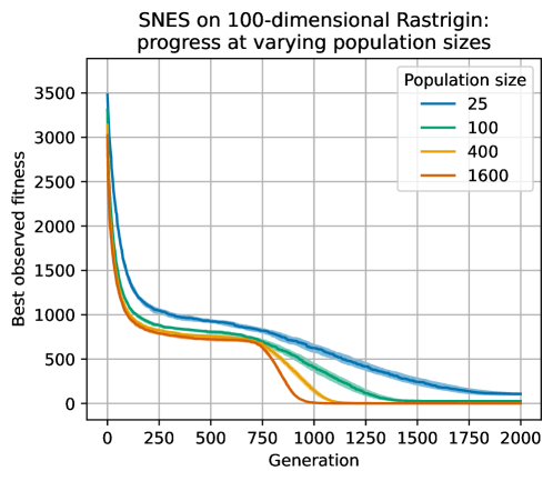
Figure 1: Comparison of the median fitness of the best solution for different population size using SNES on the 100-dimensional Rastrigin function. Bold curves represent the medians over 50 runs, and the shaded regions represent the means $\pm$ the standard deviations.

An immediate application of EvoTorch is general blackbox optimization problems. Consider the classic Rastrigin blackbox optimization benchmark function [Hoffmeister and Bäck, 1990] over $n$ dimensions,

$$f(x)=10n+\sum_{i=1}^{n}x_{i}^{2}-10\cos(2\pi x_{i}),$$ (1)

which can be implemented in vectorized form as,

⬇

@vectorized

def vrast(x: torch.Tensor) -> torch.Tensor:

return 10 * x.shape[-1] + torch.sum(x.pow(2.) - 10 * torch.cos(2 * math.pi * x), dim=-1)

which gives the vectorized and GPU-ready minimization problem,

⬇

rastrigin_prob = Problem(

"min", vrast, device="cuda:0", solution_length=100, initial_bounds=(-5.12, 5.12))

It is then straightforward to run a continuous blackbox optimization algorithm such as SNES [Schaul et al., 2011] to optimize this task,

⬇

searcher = SNES(rastrigin_prob, stdev_init=5)

searcher.run(4000) # Run for 4000 generations

.

However, note that the main measure of algorithm performance in blackbox benchmarking literature is the fitness obtained after a given budget of samples [Hansen et al., 2010]. The underlying assumption is that every sample has equal cost, but this is not strictly the case when optimization problems are vectorizable and parallelizable, which most, if not all, problems are. When time-to-solution or solution quality, rather than raw work done, is the most important criteria, vectorization and parallelization may fundamentally shift how algorithms are evaluated.

Figure 1 shows the median fitness of the best solution to the 100-dimensional Rastrigin problem discovered by SNES across 50 runs, with varying population size $\lambda\in\{25,100,400,1600\}$. Substantial increases in population size visibly improve both the speed of convergence and quality of optima discovered. However, the most surprising aspect of this is the tradeoff in computation time; in Figure 2 we present run-time performance results for the SNES implementation on both CPU and GPU. Here we observe that as the population size increases, the implementations scale elegantly into the 10s and even (in the case of GPU) hundreds of thousands.

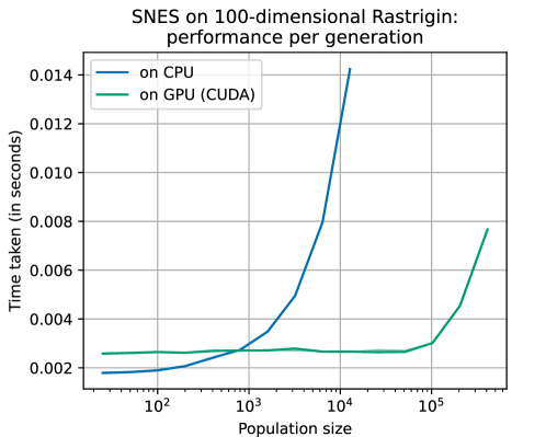
Figure 2: GPU vs CPU wall-clock time for a simple black-box optimization experiment per generation. Bold curves represent the medians, and the shaded regions represent the means $\pm$ the standard deviations. For each population size, 50 runs were started, each run lasting for 2000 generations. Median time was summarized over all generations of all runs. Therefore, each reported time for each population size is a summary over 2000 $\times$ 50 = 100000 data points.

3.2 As an alternative to first-order optimization methods

In some scenarios, one might consider using EC as an alternative to a gradient-aware first-order optimization method. One such scenario is when the fitness function is known to be differentiable, yet its implementation is only available on a framework which does not support auto-differentiation. Another such scenario is when, even though the fitness function is differentiable, the search space is nonconvex, and therefore there is a significant chance of converging to a suboptimal solution when relying on local gradients.

To be a practical alternative to first-order optimization methods, an evolutionary algorithm has to be competitive in terms of its finally converged solutions, and also in terms of its wall-clock time requirements.

Here, we evaluate the evolutionary algorithm CEM to see if it is indeed competitive against the well-known first-order optimization method Adam [Kingma and Ba, 2015]. We also add a parallelized variant of Adam into our comparison, where $n$ instances of Adam perform their searches in parallel, $n$ being the population size, equal to the population size we use for CEM.

Our test problems are the convex sphere problem ($\sum_{i\in\{1,2,...\}}x^{2}$) and the nonconvex Rastrigin problem. For each test problem, we used three settings: (i) population size=10000, dimensionality of the problem=100; (ii) population size=1000, dimensionality of the problem=1000; and (iii) population size=100, dimensionality of the problem=10000. These three settings ensure that the computations required by each iteration for each of the considered methods can be fully parallelized across the cores of a single GPU. This test, therefore, aims to demonstrate how EC compares against Adam when GPU-based parallelization is fully exploited. The results are shown in figure 3.

(a) Sphere function

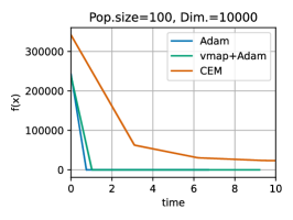
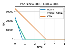
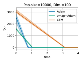
(b) Rastrigin function

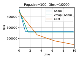
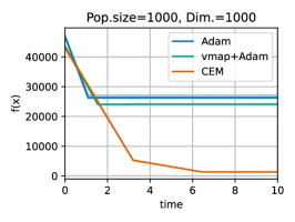
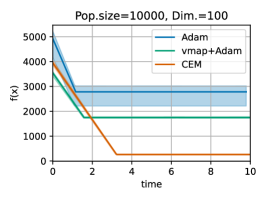
For both sphere and Rastrigin functions, initial search points were picked elementwise from within $[-10,10]$.

Hyperparameters for CEM. Initial standard deviation of the search distribution: 1.0. Parenthood ratio: 0.5 (i.e. the better half of each population is declared as parents). An element of the standard deviation vector is not allowed to change more than 2% of its original value (this limiter was previously used in the PGPE implementation of Ha [2019], where 20% was used).

Hyperparameters for Adam. Step size: 0.6 (tuned from the set $\{0.0025,0.005,0.01,0.02,0.1,0.4,0.6,1.0\}$). Other settings are left as default ($\beta_{1}=0.9$, $\beta_{2}=0.999$, $\epsilon=\textnormal{1e-8}$).

Figure 3: Convergence plots (fitness $f(x)$ vs wall clock time in seconds) comparing Adam, vmap+Adam (parallelized Adam), and CEM, on (a) sphere function and (b) Rastrigin function, considering three pairs of population sizes and problem dimensionalities. Each curve represents the median across 5 runs. Shaded regions are bounded by the means $\pm$ the standard deviations.

In figure 3(a), unsurprisingly, both variations of Adam quickly converge to the optimum point of the sphere function thanks to the accurate directions provided by the true gradients. Interestingly, we also see that the time required by CEM to converge to the optimum is in the same order of magnitude compared to the single Adam run (except when its population size is 100 where it cannot reach the optimum), despite the fact that CEM has to evaluate many test points at each iteration. This result demonstrates a case where GPU-based parallelization brings the performance of EC to a level that is comparable to first-order methods even on simple convex functions.

In figure 3(b), we see that both variations of Adam suffer from the locality of their gradients, and converge to worse local optima on the Rastrigin function compared to CEM. These results are compatible with the study of Lehman et al. [2018], where the authors show that a first-order gradient descent struggles on the "fleeting peaks" surface, a search space which has nonconvex features.

In summary, while the accuracy of the true gradients and the usefulness of the first-order methods cannot be denied, these empirical results emphasize the generality of evolutionary algorithms, and show us that GPUs further increase this generality.

3.3 multi-objective Optimization

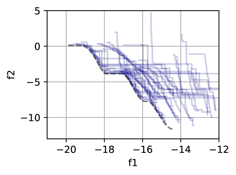
(a) Population size $25$

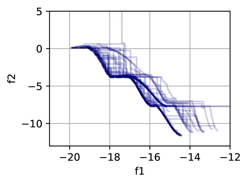
(b) Population size $100$

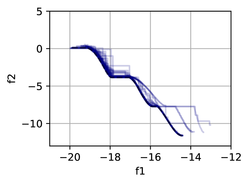
(c) Population size $400$

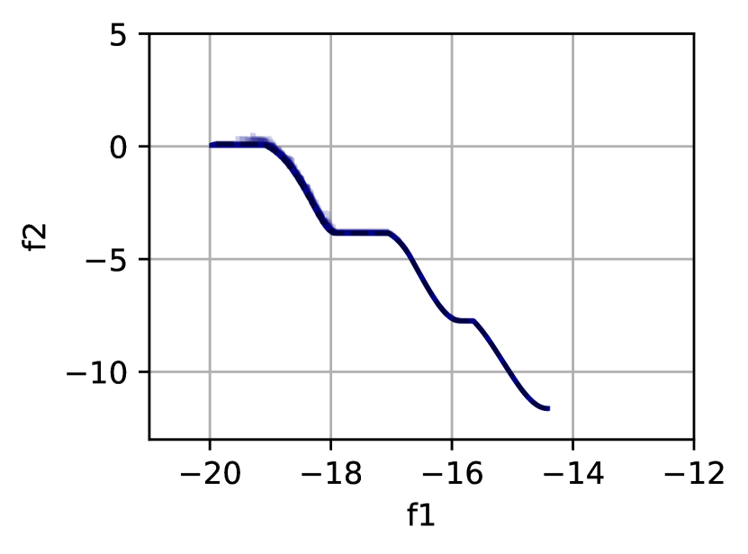
(d) Population size $1600$

Figure 4: Results for NSGA-II on the Kursawe function. Varying population sizes: (a) 25, (b) 100, (c) 400 and (d) 1600. Each faint blue line represents a Pareto front discovered by a single run of the algorithm, with 50 runs performed for each population size. The dashed black line represents the known global Pareto front of solutions.

Evolutionary algorithms are, alongside mathematical programming methods, one of the most popular approaches to a-posteriori multi-objective optimization. A specific advantage of evolutionary algorithms in this setting is that they can use membership of the Pareto front, and heuristics thereof, as a selection criteria to evolve a diverse population of candidate solutions without prior knowledge of how to weight the multiple, potentially conflicting, rewards. As a result, multi-objective evolutionary algorithms such as the NSGA family [Deb et al., 2002; Deb and Jain, 2013], MOEA/D Zhang and Li [2007] and AGE-MOEA [Panichella, 2019] have found widespread application, for example in planning [Sarker and Ray, 2009], molecular docking [Janson et al., 2008] and neural architecture search [Lu et al., 2019].

EvoTorch facilitates the straight-forward implementation and application of multi-objective optimization at scale. By default, EvoTorch problem definitions support multiple objectives. Consider the bi-objective, tri-variate Kursawe function [Kursawe, 1990],

$$f_{1}(x)=\sum_{i=1}^{2}-10e^{-0.2\sqrt{x_{i}^{2}+x_{i+1}^{2}}},$$ (2)

$$f_{2}(x)=\sum_{i=1}^{3}|x_{i}|^{0.8}+5\sin x_{i}^{3}.$$ (3)

This function can be easily implemented in vectorized form using PyTorch such that the declared function receives a $(k,3)$ dimensional tensor of $k$ 3-dimensional vector solutions, and returns a $(k,2)$ dimensional tensor of $k$ 2-dimensional fitnesses:

⬇

@vectorized

def kursawe(x: torch.Tensor) -> torch.Tensor:

f1 = torch.sum(

-10 * torch.exp(

-0.2 * torch.sqrt(x[:, 0:2] ** 2.0 + x[:, 1:3] ** 2.0)

),

dim=-1,

) # Compute the first objective

f2 = torch.sum(

(torch.abs(x) ** 0.8) + (5 * torch.sin(x ** 3)),

dim=-1,

) # Compute the second objective

fitnesses = torch.stack([f1, f2], dim=-1) # Stack the two objectives together

return fitnesses

Then a problem class can be instantiated as normal,

⬇

kursawe_prob = Problem(

["min", "min"], kursawe, # Both objectives are to be minimized

solution_length=3,

initial_bounds=(-5.0, 5.0),

solution_length=3,

)

The genetic algorithm implementation of EvoTorch can handle multiple objectives, and therefore can work on kursawe_prob:

⬇

ga = GeneticAlgorithm(kursawe_prob, popsize=...)

When initialized with a multi-objective problem, GeneticAlgorithm follows the procedures of NSGA-II [Deb et al., 2002] and enables the behavior of organizing its populations using Pareto-ranking and crowd-sorting.

Figure 4 shows the results of running this multi-objective algorithm for $30$ generations with varying population sizes. Each faint line represents the Pareto front of discovered solutions by the algorithm, with 50 runs performed for each population size. Even though the total number of generations remains the same, it can clearly be seen that increasing the population size yields substantially better Pareto fronts, with the $1600$ population size reliably obtaining the known global optimum for this problem, represented as a black dashed line in each plot.

While scaling the population is clearly beneficial for NSGA-II, in principle, many multi-objective evolutionary algorithms require $O(n^{2})$ time complexity where $n$ is the population size, as they require pairwise comparisons of the individual solutions’ fitness values to establish Pareto dominance. In practice, this computationally limits the application of MOEAs to relatively small population sizes. However, the underlying mathematics of computing population-wide pareto dominance are highly vectorizable and therefore well-suited to execution on accelerated hardware such as GPUs.

As a result, when excluding the time complexity of fitness evaluation which may vary with application, we generally observe that the run-time of EvoTorch’s NSGA-II implementation scales elegantly with the population size when deployed on such accelerated hardware. This is demonstrated in Figure 5, where NSGA-II is run on the Kursawe problem at varying population sizes on both the CPU and GPU. In this setting, we observe that we are able to efficiently run NSGA-II on the GPU with population sizes greater than $10000$, thanks to the fast implementation of Pareto sorting.

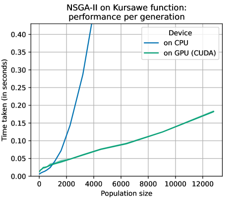
Figure 5: GPU vs CPU wall-clock times for a simple multi-objective optimization experiment per generation. Bold curves represent the medians, and the shaded regions represent the means $\pm$ the standard deviations. For each population size, 50 runs were started, each run lasting for 30 generations. Median time was summarized over all generations of all runs. Therefore, each reported time for each population size is a summary over 30 $\times$ 50 = 1500 data points.

3.4 Reinforcement learning

It has been demonstrated that evolutionary algorithms are competitive for solving reinforcement learning tasks (see, e.g., [Salimans et al., 2017; Mania et al., 2018; Ha, 2019]). EvoTorch provides problem types for tackling gym and brax tasks. Additionally, utilities which were demonstrated by Salimans et al. [2017] as helpful for evolutionary reinforcement learning, such as online observation normalization and adaptive population size, are also implemented.

3.4.1 Gym

The gym library [Brockman et al., 2016] provides various reinforcement learning tasks that have been used as common benchmarks. Among the environments provided by gym are continuous locomotion tasks (such as hopper [Erez et al., 2011], walker, humanoid [Tassa et al., 2012], etc.) based on the MuJoCo simulator [Todorov et al., 2012]. Additional gym environments can be provided by libraries such as PyBullet [Coumans and Bai, 2021], Roboschool [Klimov and Schulman, 2017], PyBullet Gymperium [Ellenberger, 2019], etc.

EvoTorch has a problem type named GymNE for solving reinforcement learning tasks defined by the gym library. A simple instantiation of GymNE for solving the cart pole task looks like this:

⬇

from evotorch.neuroevolution import GymNE

problem = GymNE(env="CartPole-v1", network=network_class)

where network_class is a reference to a class that inherits from torch.nn.Module, which specifies the architecture of the neural network whose parameters will be evolved. More keyword arguments are available for enabling observation normalization, multi-episode evaluation, hard-coded alive bonus removal (which is reported to help with standard locomotion benchmarks [Mania et al., 2018; Toklu et al., 2020]), timestep-dependent manual alive bonus schedule, parallelized evaluation (using multiple actors via num_actors), etc.

It has been observed that the PGPE+ClipUp (i.e. PGPE [Sehnke et al., 2010] coupled with the ClipUp optimizer [Toklu et al., 2020]) implementation of EvoTorch can solve the MuJoCo tasks Walker2d-v4 and Humanoid-v4 with a performance that is compatible with [Toklu et al., 2020]. We have also observed that the PyBullet task HumanoidBulletEnv-v0 can be solved to obtain a competitive cumulative reward. The results are shown in figure 6.

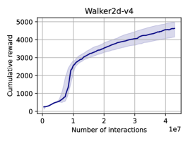
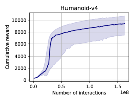
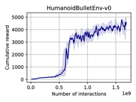
Configuration. For Walker2d-v4 and Humanoid-v4, linear policies with bias terms were used. For HumanoidBulletEnv-v0, a neural network with a hidden recurrent layer of 64 neurons and with tanh activations was used. For each task, PGPE+ClipUp hyperparameters were taken from [Toklu et al., 2020]. In the case of HumanoidBulletEnv-v0, even though a non-recurrent network was used in [Toklu et al., 2020], same hyperparameters were used and observed to work for the runs reported here with recurrent policies.

Figure 6: Results obtained on locomotion tasks with PGPE+ClipUp. The plots for Walker2d-v4 and Humanoid-v4 summarize 30 runs. The plot for HumanoidBulletEnv-v0 summarizes 5 runs. In each plot, bold curve represents the median and the shaded area is bounded by the mean $\pm$ the standard deviation.

3.4.2 Brax

brax [Freeman et al., 2021b, a] is a differentiable and vectorized simulator written in JAX that can take advantage of hardware accelerators including GPUs. EvoTorch provides a vectorized counterpart of GymNE named VecGymNE, that can work with brax tasks.

We performed test runs using PGPE+ClipUp on a single GPU for solving the brax tasks fetch and humanoid. The results are shown in figure 7. In the figure, we see that, in the median case, the cumulative reward threshold 12 can be reached in less than 14 minutes for the fetch task. In the case of the humanoid task, if we accept 6000 as the solving threshold for the humanoid task (as done for its MuJoCo counterpart, Humanoid-v4, in e.g. [Salimans et al., 2017; Mania et al., 2018]), we see that interesting locomotion behaviors are learned in less than 6 minutes in the median case. We also see that a cumulative reward around 10000 can be achieved for the humanoid task after 100 generations.

(a) fetch

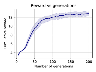
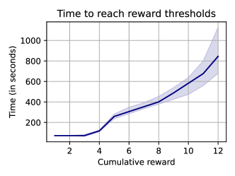
Policy: A neural network with a single hidden recurrent layer of 64 neurons, with tanh activations. An elementwise non-affine layer normalization is applied just before the output layer. The output layer is a linear transformation, followed by a clip operation to make sure that the produced output is within valid boundaries.

(b) humanoid

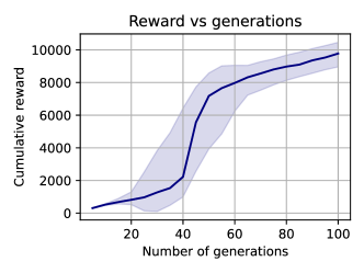
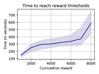
Policy: A linear policy with bias terms. Alive bonus: The default constant alive bonus of 5.0 (which has been reported to harm exploration for distribution-based evolutionary search [Mania et al., 2018; Toklu et al., 2020]) is removed. Instead, here we used a timestep-dependent alive bonus schedule: from timestep 0 to 400, the agent receives no alive bonus; from timestep 400 to 700, the alive bonus linearly increases from 0.0 to 10.0; and beginning with timestep 700, the agent receives an alive bonus of 10.0 for each timestep. By this tuning, we aim to make the alive bonus an active component of the reward function only towards the later phases of the evolution where the agents have learned to walk and their episodes are longer.

PGPE+ClipUp configuration for both (a) and (b). We enabled two enhancements previously used by [Salimans et al., 2017]: observation normalization and 0-centered solution ranking (where the worst solution is assigned the rank -0.5 and the best solution is assigned the rank +0.5). Population size: 12000; center learning rate: 0.375; maximum speed for ClipUp: 0.75; standard deviation learning rate: 0.1.

Figure 7: Results obtained on brax tasks with PGPE+ClipUp. Each plot summarizes 30 runs. In each plot, bold curve represents the median and the shaded area is bounded by the mean $\pm$ the standard deviation.

3.5 Supervised learning

There is a broad interest in applying evolutionary algorithms to supervised learning tasks, for example as an alternative to gradient-based methods for training neural networks for regression and classification [Mandischer, 2002; Zhang et al., 2017; Lehman et al., 2018; Lenc et al., 2019; Li et al., 2019]. Beyond simply serving as an alternative to gradient-descent, EA-based approaches to supervised learning open up a number of interesting research directions, such as training on inference-only hardware, optimizing for non-differentiable or discontinuous loss functions and optimizing non-differentiable neural architectures. To facilitate these research directions, EvoTorch provides support for supervised neuroevolution out-of-the-box through the SupervisedNE problem class.

To demonstrate this, we consider the experiments presented in [Lenc et al., 2019], specifically for training a small convolutional neural network on the MNIST dataset. We use ‘MNIST30K’ network as described, except that we use layer normalization rather than batch normalization. With this network defined as a PyTorch module class MNIST30K, and with a training dataset train_dataset prepared, creation of a problem instance is then straight-forward:

⬇

mnist_problem = SupervisedNE(

train_dataset, # Using the mnist training dataset

MNIST30K, # Training the MNIST30K module

nn.CrossEntropyLoss(), # Minimizing cross-entropy loss

minibatch_size=1024, # With a minibatch size of 512

common_minibatch=True, # Always using the same minibatch across all solutions on an actor

num_actors=32, # The total number of CPUs used

num_gpus_per_actor=’max’, # Dividing all available GPUs between the 32 actors

)

In this configuration, 32 ray actors will be created, each with a fragment of a GPU assigned to it, for the forward (inference) step of evaluating each member of the population under cross-entropy loss across 1024 samples. As noted in Lenc et al. [2019], gradient updates can be more stable when the same minibatch of data is used across all solutions evaluated by a single actor within a single step; this is reflected in the common_minibatch argument.

This problem class can be interfaced by search algorithms like any other. In this example, we use the PGPE search algorithm with the Adam optimizer and a population size of 3200. We generally found that raw fitnesses could be used directly, rather than rank-based fitness shaping, to beneficial effect. Additionally, as described by Lenc et al. [2019] as ‘semi-updates’, the gradients used by distribution-based evolutionary algorithms can be approximated locally on individual actors and then averaged without introducing any bias; this is reflected in the distributed argument. Our search algorithm is therefore instantiated:

⬇

searcher = PGPE(

mnist_problem,

radius_init=2.25, # Initial radius of the search distribution

center_learning_rate=1e-2, # Learning rate used by adam optimizer

stdev_learning_rate=0.1, # Learning rate for the standard deviation

popsize=3200,

distributed=True, # Gradients are computed locally at actors and averaged

optimizer=’adam’, # Using the adam optimizer

ranking_method=None, # No rank-based fitness shaping is used

)

Running the evolutionary algorithm for only $400$ generations, we observe quick convergence in the training loss as shown in Figure 8. Once we have allowed the search algorithm to converge, we obtain a respectable $98.8\%$ test accuracy on unseen data.

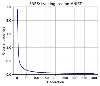
Figure 8: Training loss (cross entropy) of a single run of SNES on the MNIST dataset by generation. The loss shown is the mean of the loss obtained by each member of the population in each generation.

3.6 Discrete Optimization

In EvoTorch, the data type of the decision variables can be declared as integer (e.g. torch.int32, torch.int64, etc.) or boolean (i.e. torch.bool). Assuming the goal of minimization, defining a discrete optimization problem looks like this:

⬇

discrete_problem = Problem("min", discrete_fitness_function, dtype=torch.int64, ...)

where discrete_fitness_function is expected as a function which receives a tensor whose dtype is torch.int64 and returns a fitness tensor whose dtype is a floating-point type (torch.float32 by default).

Such problems with discrete decision variable types can be solved with GeneticAlgorithm. EvoTorch provides implementations of cross-over operators for GeneticAlgorithm that are friendly with discrete variable types. Problem-specific mutation operators can be defined by the user. A GeneticAlgorithm instantiation for discrete_problem looks like this:

⬇

from evotorch.operators import TwoPointCrossOver

def mutate(decision_values: torch.Tensor) -> torch.Tensor:

# Here, decision_values is a 2-dimensional tensor where each row represents a solution.

mutated_decision_values = ... # a mutated copy of decision_values is generated here

return mutated_decision_values

ga = GeneticAlgorithm(

discrete_problem,

operators=[TwoPointCrossOver(discrete_problem), mutate],

popsize=...,

...

)

Challenges regarding vectorization. In many discrete optimization problems, straightforward vectorization might not be possible because the fitness functions must be expressed algorithmically (rather than as combinations of numeric PyTorch operations). An important example comes from the field of genetic programming where fitness functions interpret executable programs encoded in the candidate solutions. This interpreter must visit each symbol of the given program sequentially, perform conditional operations according to the symbol at hand, and produce the final result only at the end of the program. It is this algorithmic and sequential nature that hinders the vectorization across the decision variables of a batch of solutions. However, this does not mean that vectorization is hindered entirely. Indeed, there can be a vectorized interpreter which, within a single step, processes the next symbol of each program. Therefore, more generally, while algorithmic and/or sequential fitness functions might sacrifice vectorization across the decision variables, it can still be enjoyed across multiple solutions.

To allow the user to express sequential fitness functions in a practical manner, EvoTorch provides vectorized PyTorch-based data structures that can be used as variable length lists, queues, stacks, and dictionaries. As an example, let us imagine that we have 10000 lists. Considering each of these lists, let us say we wish to sample a real number, and then, if the sampled number is positive, we wish to append it into its associated list. This program can be written without writing any loop as follows:

⬇

from evotorch.tools.structures import CList

batch_of_lists = CList( # make a batch of lists with contiguous storage

max_length=10, # each list can have at most this many elements

batch_size=10000, # we want this many lists in our batch

# device="cuda", # can be enabled for exploiting the GPU

)

batch_of_numbers = torch.randn(10000, device=batch_of_lists.device)

batch_of_lists.append_(batch_of_numbers, where=(batch_of_numbers > 0))

A genetic programming example has been implemented where the fitness function is a stack-based interpreter written using the CList structure. Populations ranged from 5000 to 100000 programs of maximum length 20. Wall-clock times were compared for a single GPU versus a 40-thread CPU (without multiple actors, with multithreading enabled for PyTorch). The results in figure 9 show that the GPU time requirement is almost flat up to population size 30000, whereas the CPU curve increases sharply, taking more than 10 times that the GPU implementation for population size 10000.

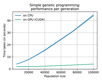
Figure 9: GPU vs CPU wall-clock times for a simple genetic programming notebook per generation. Bold curves represent the medians, and the shaded regions represent the means $\pm$ the standard deviations. For each population size, 30 runs were started, each run lasting for 50 generations. Median time was summarized over all generations (except the very first generation where the population initialization procedures have an overhead) of all runs. Therefore, each reported time for each population size is a summary over 49 $\times$ 30 = 1470 data points.

Although we have used genetic programming as our example, we argue that fitness functions of similar nature might be encountered in other discrete optimization fields such as transportation, scheduling, etc. It is our hope that the features of EvoTorch mentioned here can allow the users to quickly prototype GPU-friendly problem definitions in such cases.

4 Conclusion

We have presented EvoTorch, an evolutionary computation library written in Python programming language and built upon PyTorch and ray. Among the highlights of the library are:

• seamless interaction with the well-developed scientific ecosystem of Python;

• ability to exploit hardware accelerators such as GPU with the help of PyTorch;

• ability to scale up to large experiments with the help of CPU-based parallelization and distributed computation abilities brought by ray;

• efficient neuroevolution and blackbox optimization thanks to having state-of-the-art algorithm implementations (PGPE, XNES, etc.);

• general abilities to address various types of problems (with single or multiple objectives, with continuous or discrete variable types, etc.).

It is our hope that EvoTorch will become a practical tool for performing large-scale evolutionary computation in both the research and industrial communities.

References

-
Abadi et al. [2016]
Abadi, M., P. Barham, J. Chen, Z. Chen, A. Davis, J. Dean, M. Devin,
S. Ghemawat, G. Irving, M. Isard, M. Kudlur, J. Levenberg, R. Monga,
S. Moore, D. G. Murray, B. Steiner, P. Tucker, V. Vasudevan, P. Warden,
M. Wicke, Y. Yu, and X. Zheng
2016. TensorFlow: A system for large-scale machine learning. In 12th USENIX Symposium on Operating Systems Design and Implementation (OSDI 16), Pp. 265–283. Available online: https://www.usenix.org/system/files/conference/osdi16/osdi16-abadi.pdf. -
Back and Schwefel [1996]
Back, T. and H.-P. Schwefel
1996. Evolutionary computation: An overview. In Proceedings of IEEE International Conference on Evolutionary Computation, Pp. 20–29. IEEE. doi:10.1109/ICEC.1996.542329. -
Biscani and Izzo [2020]
Biscani, F. and D. Izzo
2020. A parallel global multiobjective framework for optimization: pagmo. Journal of Open Source Software, 5(53):2338. -
Blank and Deb [2020]
Blank, J. and K. Deb
2020. Pymoo: Multi-objective optimization in Python. IEEE Access, 8:89497–89509. doi:10.1109/ACCESS.2020.2990567. -
Brockman et al. [2016]
Brockman, G., V. Cheung, L. Pettersson, J. Schneider, J. Schulman, J. Tang, and
W. Zaremba
2016. Openai gym. arXiv preprint. arXiv:1606.01540. -
Chellapilla et al. [2006]
Chellapilla, K., S. Puri, and P. Simard
2006. High performance convolutional neural networks for document processing. In Tenth international workshop on frontiers in handwriting recognition (IWFHR 10). hal:inria-00112631. -
Ciresan et al. [2011]
Ciresan, D. C., U. Meier, J. Masci, L. M. Gambardella, and
J. Schmidhuber
2011. Flexible, high performance convolutional neural networks for image classification. In Proceedings of the Twenty-Second International Joint Conference on Artificial Intelligence (IJCAI’11), Pp. 1237–1242. AAAI Press. Available online: https://www.aaai.org/ocs/index.php/IJCAI/IJCAI11/paper/view/3098/3425. -
Coumans and Bai [2021]
Coumans, E. and Y. Bai
2016–2021. Pybullet, a python module for physics simulation for games, robotics and machine learning. http://pybullet.org. -
Deb and Jain [2013]
Deb, K. and H. Jain
2013. An evolutionary many-objective optimization algorithm using reference-point-based nondominated sorting approach, part I: solving problems with box constraints. IEEE Transactions on Evolutionary Computation (TEVC), 18(4):577–601. doi:10.1109/TEVC.2013.2281535. -
Deb et al. [2002]
Deb, K., A. Pratap, S. Agarwal, and T. Meyarivan
2002. A fast and elitist multiobjective genetic algorithm: NSGA-II. IEEE Transactions on Evolutionary Computation (TEVC), 6(2):182–197. doi:10.1109/4235.996017. -
Ellenberger [2019]
Ellenberger, B.
2018–2019. Pybullet gymperium. https://github.com/benelot/pybullet-gym. -
Erez et al. [2011]
Erez, T., Y. Tassa, and E. Todorov
2011. Infinite-horizon model predictive control for periodic tasks with contacts. In Proceedings of Robotics: Science and Systems VII. MIT Press. doi:10.15607/RSS.2011.VII.010. -
Fey and Lenssen [2019]
Fey, M. and J. E. Lenssen
2019. Fast graph representation learning with pytorch geometric. arXiv preprint. arXiv:1903.02428. -
Fortin et al. [2012]
Fortin, F.-A., F.-M. De Rainville, M.-A. G. Gardner, M. Parizeau, and
C. Gagné
2012. DEAP: Evolutionary algorithms made easy. Journal of Machine Learning Research (JMLR), 13(1):2171–2175. Available online: https://www.jmlr.org/papers/v13/fortin12a.html. -
Freeman et al. [2021a]
Freeman, C. D., E. Frey, A. Raichuk, S. Girgin, I. Mordatch, and
O. Bachem
2021a. Brax - a differentiable physics engine for large scale rigid body simulation. http://github.com/google/brax. -
Freeman et al. [2021b]
Freeman, C. D., E. Frey, A. Raichuk, S. Girgin, I. Mordatch, and
O. Bachem
2021b. Brax–a differentiable physics engine for large scale rigid body simulation. arXiv preprint. arXiv:2106.13281. -
Frostig et al. [2018]
Frostig, R., M. J. Johnson, and C. Leary
2018. Compiling machine learning programs via high-level tracing. Systems for Machine Learning, 4(9). Available online: https://mlsys.org/Conferences/doc/2018/146.pdf. -
Gardner et al. [2017]
Gardner, M., J. Grus, M. Neumann, O. Tafjord, P. Dasigi, N. F. Liu, M. Peters,
M. Schmitz, and L. S. Zettlemoyer
2017. Allennlp: A deep semantic natural language processing platform. arXiv preprint. arXiv:1803.07640. -
GitHub [2023a]
GitHub
2023a. Contributors to nnaisense/evotorch. https://github.com/nnaisense/evotorch/graphs/contributors. -
GitHub [2023b]
GitHub
2023b. Issues nnaisense/evotorch. https://github.com/nnaisense/evotorch/issues. -
Glasmachers et al. [2010]
Glasmachers, T., T. Schaul, S. Yi, D. Wierstra, and
J. Schmidhuber
2010. Exponential natural evolution strategies. In Proceedings of the 12th annual conference on Genetic and Evolutionary Computation (GECCO’10), Pp. 393–400. ACM. doi:10.1145/1830483.1830557. -
Gomez et al. [2008]
Gomez, F., J. Schmidhuber, R. Miikkulainen, and
M. Mitchell
2008. Accelerated neural evolution through cooperatively coevolved synapses. Journal of Machine Learning Research, 9(5). Available online: https://www.jmlr.org/papers/v9/gomez08a.html. -
Greff et al. [2017]
Greff, K., A. Klein, M. Chovanec, F. Hutter, and
J. Schmidhuber
2017. The Sacred Infrastructure for Computational Research. In Proceedings of the 16th Python in science conference (SciPy 2017), Pp. 49–56. doi:10.25080/shinma-7f4c6e7-008. -
Ha [2019]
Ha, D.
2019. Reinforcement learning for improving agent design. Artificial Life, 25(4):352–365. doi:10.1162/artl_a_00301. -
Hansen et al. [2010]
Hansen, N., A. Auger, R. Ros, S. Finck, and
P. Pošík
2010. Comparing results of 31 algorithms from the black-box optimization benchmarking BBOB-2009. In Proceedings of the 12th annual conference on Genetic and Evolutionary Computation (GECCO’10), Pp. 1689–1696. ACM. doi:10.1145/1830761.1830790. -
Hansen and Ostermeier [2001]
Hansen, N. and A. Ostermeier
2001. Completely derandomized self-adaptation in evolution strategies. Evolutionary computation, 9(2):159–195. doi:10.1162/106365601750190398. -
Hoffmeister and
Bäck [1990]
Hoffmeister, F. and T. Bäck
1990. Genetic algorithms and evolution strategies: Similarities and differences. In International Conference on Parallel Problem Solving from Nature (PPSN 1990), Pp. 455–469. Springer. doi:10.1007/bfb0029787. -
Holland [1975]
Holland, J.
1975. Adaptation in Natural and Artificial Systems. University of Michigan Press. doi:10.7551/mitpress/1090.001.0001. -
Holland [1992]
Holland, J. H.
1992. Genetic algorithms. Scientific american, 267(1):66–73. Available online: https://www.jstor.org/stable/24939139. -
Huang et al. [2023]
Huang, B., R. Cheng, Y. Jin, and K. C. Tan
2023. EvoX: A distributed GPU-accelerated library towards scalable evolutionary computation. arXiv preprint. arXiv:2301.12457. -
Innes [2018]
Innes, M.
2018. Flux: Elegant machine learning with Julia. Journal of Open Source Software, 3(25):602. doi:10.21105/joss.00602. -
James Bergstra et al. [2010]
James Bergstra, Olivier Breuleux, Frédéric Bastien, Pascal
Lamblin, Razvan Pascanu, Guillaume Desjardins, Joseph Turian,
David Warde Farley, and Yoshua
Bengio
2010. Theano: a cpu and gpu math compiler in Python. In Proceedings of the 9th Python in science conference (SciPy 2010), Pp. 18 – 24. doi:10.25080/Majora-92bf1922-003. -
Janson et al. [2008]
Janson, S., D. Merkle, and M. Middendorf
2008. Molecular docking with multi-objective particle swarm optimization. Applied Soft Computing, 8(1):666–675. doi:10.1016/j.asoc.2007.05.005. -
Kingma and Ba [2015]
Kingma, D. P. and J. Ba
2015. Adam: A method for stochastic optimization. In Proceedings of 3rd International Conference on Learning Representations (ICLR). arXiv:1412.6980. -
Klimov and Schulman [2017]
Klimov, O. and J. Schulman
2017. Roboschool. https://openai.com/blog/roboschool/. -
Krizhevsky et al. [2012]
Krizhevsky, A., I. Sutskever, and G. E. Hinton
2012. ImageNet classification with deep convolutional neural networks. Advances in neural information processing systems (NIPS 2012), 25. Available online: https://proceedings.neurips.cc/paper/2012/file/c399862d3b9d6b76c8436e924a68c45b-Paper.pdf. -
Kursawe [1990]
Kursawe, F.
1990. A variant of evolution strategies for vector optimization. In International conference on parallel problem solving from nature (PPSN 1990), Pp. 193–197. Springer. doi:10.1007/BFb0029752. -
Lange [2022]
Lange, R. T.
2022. evosax: Jax-based evolution strategies. arXiv preprint. arXiv:2212.04180. -
Lehman et al. [2018]
Lehman, J., J. Chen, J. Clune, and K. O. Stanley
2018. ES is more than just a traditional finite-difference approximator. In Proceedings of the 16th annual conference on Genetic and Evolutionary Computation (GECCO’18), Pp. 450–457. doi:10.1145/3205455.3205474. -
Lenc et al. [2019]
Lenc, K., E. Elsen, T. Schaul, and K. Simonyan
2019. Non-differentiable supervised learning with evolution strategies and hybrid methods. arXiv preprint. arXiv:1906.03139. -
Li et al. [2019]
Li, Y., Z. Zhu, D. Kong, H. Han, and Y. Zhao
2019. EA-LSTM: Evolutionary attention-based LSTM for time series prediction. Knowledge-Based Systems, 181:104785. doi:10.1016/j.knosys.2019.05.028. -
Lu et al. [2019]
Lu, Z., I. Whalen, V. Boddeti, Y. Dhebar, K. Deb, E. Goodman, and
W. Banzhaf
2019. NSGA-net: neural architecture search using multi-objective genetic algorithm. In Proceedings of the 17th annual conference on Genetic and Evolutionary Computation (GECCO’19), Pp. 419–427. doi:10.1145/3321707.3321729. -
Luke [1998]
Luke, S.
1998. ECJ evolutionary computation library. Available for free at http://cs.gmu.edu/~eclab/projects/ecj/. -
Mandischer [2002]
Mandischer, M.
2002. A comparison of evolution strategies and backpropagation for neural network training. Neurocomputing, 42(1-4):87–117. doi:10.1016/S0925-2312(01)00596-3. -
Mania et al. [2018]
Mania, H., A. Guy, and B. Recht
2018. Simple random search of static linear policies is competitive for reinforcement learning. In Advances in Neural Information Processing Systems (NeurIPS 2018), Pp. 1800–1809. Available online: https://proceedings.neurips.cc/paper/2018/file/7634ea65a4e6d9041cfd3f7de18e334a-Paper.pdf. -
MLflow Contributors [2022]
MLflow Contributors
2022. mlflow: Open source platform for the machine learning lifecycle. https://github.com/mlflow/mlflow. -
Moritz et al. [2018]
Moritz, P., R. Nishihara, S. Wang, A. Tumanov, R. Liaw, E. Liang, M. Elibol,
Z. Yang, W. Paul, M. I. Jordan, and I. Stoica
2018. Ray: A distributed framework for emerging AI applications. In 13th USENIX Symposium on Operating Systems Design and Implementation (OSDI 18), Pp. 561–577. -
Mouret and Clune [2015]
Mouret, J.-B. and J. Clune
2015. Illuminating search spaces by mapping elites. arXiv preprint. arXiv:1504.04909. -
Neptune Contributors [2022]
Neptune Contributors
2022. neptune-client: Experiment tracking tool and model registry. https://github.com/neptune-ai/neptune-client. -
Panichella [2019]
Panichella, A.
2019. An adaptive evolutionary algorithm based on non-euclidean geometry for many-objective optimization. In Proceedings of the 17th annual conference on Genetic and Evolutionary Computation (GECCO’19), Pp. 595–603. doi:10.1145/3321707.3321839. -
Paszke et al. [2019]
Paszke, A., S. Gross, F. Massa, A. Lerer, J. Bradbury, G. Chanan, T. Killeen,
Z. Lin, N. Gimelshein, L. Antiga, A. Desmaison, A. Kopf, E. Yang, Z. DeVito,
M. Raison, A. Tejani, S. Chilamkurthy, B. Steiner, L. Fang, J. Bai, and
S. Chintala
2019. PyTorch: An imperative style, high-performance deep learning library. In Advances in Neural Information Processing Systems (NeurIPS 2019), volume 32. Available online: https://proceedings.neurips.cc/paper/2019/file/bdbca288fee7f92f2bfa9f7012727740-Paper.pdf. -
Rubinstein [1999]
Rubinstein, R.
1999. The cross-entropy method for combinatorial and continuous optimization. Methodology and computing in applied probability, 1(2):127–190. doi:10.1023/A:1010091220143. -
Rubinstein [1997]
Rubinstein, R. Y.
1997. Optimization of computer simulation models with rare events. European Journal of Operational Research, 99(1):89–112. doi:10.1016/S0377-2217(96)00385-2. -
Salimans et al. [2017]
Salimans, T., J. Ho, X. Chen, S. Sidor, and
I. Sutskever
2017. Evolution strategies as a scalable alternative to reinforcement learning. arXiv preprint arXiv. arXiv:1703.03864. -
Sarker and Ray [2009]
Sarker, R. and T. Ray
2009. An improved evolutionary algorithm for solving multi-objective crop planning models. Computers and electronics in agriculture, 68(2):191–199. doi:10.1016/j.compag.2009.06.002. -
Schaul et al. [2011]
Schaul, T., T. Glasmachers, and J. Schmidhuber
2011. High dimensions and heavy tails for natural evolution strategies. In Proceedings of the 13th annual conference on Genetic and Evolutionary Computation (GECCO’11), Pp. 845–852. doi:10.1145/2001576.2001692. -
Schmidhuber [2015]
Schmidhuber, J.
2015. Deep learning in neural networks: An overview. Neural networks, 61:85–117. doi:10.1016/j.neunet.2014.09.003. -
Sehnke et al. [2010]
Sehnke, F., C. Osendorfer, T. Rückstieß, A. Graves, J. Peters, and
J. Schmidhuber
2010. Parameter-exploring policy gradients. Neural Networks, 23(4):551–559. doi:10.1016/j.neunet.2009.12.004. -
Tang et al. [2022]
Tang, Y., Y. Tian, and D. Ha
2022. EvoJAX: Hardware-accelerated neuroevolution. arXiv preprint. arXiv:2202.05008. -
Tassa et al. [2012]
Tassa, Y., T. Erez, and E. Todorov
2012. Synthesis and stabilization of complex behaviors through online trajectory optimization. In Proceedings of the IEEE/RSJ International Conference on Intelligent Robots and Systems, Pp. 4906–4913. IEEE. doi:10.1109/IROS.2012.6386025. -
Todorov et al. [2012]
Todorov, E., T. Erez, and Y. Tassa
2012. Mujoco: A physics engine for model-based control. In Proceedings of the IEEE/RSJ International Conference on Intelligent Robots and Systems, Pp. 5026–5033. IEEE. doi:10.1109/IROS.2012.6386109. -
Toklu et al. [2020]
Toklu, N. E., P. Liskowski, and R. K. Srivastava
2020. Clipup: a simple and powerful optimizer for distribution-based policy evolution. In International Conference on Parallel Problem Solving from Nature (PPSN 2020), Pp. 515–527. Springer. doi:10.1007/978-3-030-58115-2_36. -
Tokui et al. [2015]
Tokui, S., K. Oono, S. Hido, and J. Clayton
2015. Chainer: a next-generation open source framework for deep learning. In Proceedings of workshop on Machine Learning Systems (LearningSys) in Advances in Neural information processing systems (NIPS 2015), volume 5, Pp. 1–6. Available online: http://learningsys.org/papers/LearningSys_2015_paper_33.pdf. -
Van Rossum and Drake [2009]
Van Rossum, G. and F. L. Drake
2009. Python 3 Reference Manual. CreateSpace. Available online: https://docs.python.org/3/reference/. -
Wu et al. [2019]
Wu, Y., A. Kirillov, F. Massa, W.-Y. Lo, and
R. Girshick
2019. Detectron2. https://github.com/facebookresearch/detectron2. -
Yuret [2016]
Yuret, D.
2016. Knet: Beginning deep learning with 100 lines of Julia. In Proceedings of workshop on Machine Learning Systems (LearningSys) in Advances in Neural information processing systems (NIPS 2016), volume 2016, P. 5. Available online: https://www.vliz.be/nl/kaarten-bibliotheek?module=ref&refid=310930. -
Zhang and Li [2007]
Zhang, Q. and H. Li
2007. MOEA/D: A multiobjective evolutionary algorithm based on decomposition. IEEE Transactions on evolutionary computation (TEVC), 11(6):712–731. doi:10.1109/TEVC.2007.892759. -
Zhang et al. [2017]
Zhang, X., J. Clune, and K. O. Stanley
2017. On the relationship between the OpenAI evolution strategy and stochastic gradient descent. arXiv preprint. arXiv:1712.06564. -
Zhu et al. [2022]
Zhu, Z., C. Shi, Z. Zhang, S. Liu, M. Xu, X. Yuan, Y. Zhang, J. Chen, H. Cai,
J. Lu, C. Ma, R. Liu, L.-P. Xhonneux, M. Qu, and
J. Tang
2022. Torchdrug: A powerful and flexible machine learning platform for drug discovery. arXiv preprint. arXiv:2202.08320.