Uncovering gravitational-wave backgrounds from noises of unknown shape with LISA

Abstract

Detecting stochastic background radiation of cosmological origin is an exciting possibility for current and future gravitational-wave (GW) detectors. However, distinguishing it from other stochastic processes, such as instrumental noise and astrophysical backgrounds, is challenging. It is even more delicate for the space-based GW observatory LISA since it cannot correlate its observations with other detectors, unlike today’s terrestrial network. Nonetheless, with multiple measurements across the constellation and high accuracy in the noise level, detection is still possible. In the context of GW background detection, previous studies have assumed that instrumental noise has a known, possibly parameterized, spectral shape. To make our analysis robust against imperfect knowledge of the instrumental noise, we challenge this crucial assumption and assume that the single-link interferometric noises have an arbitrary and unknown spectrum. We investigate possible ways of separating instrumental and GW contributions by using realistic LISA data simulations with time-varying arms and second-generation time-delay interferometry. By fitting a generic spline model to the interferometer noise and a power-law template to the signal, we can detect GW stochastic backgrounds up to energy density levels comparable with fixed-shape models. We also demonstrate that we can probe a region of the GW background parameter space that today’s detectors cannot access.

I Introduction

The hunt for stochastic gravitational-wave backgrounds (SGWBs) (see [1, 2, 3, 4, 5, 6, 7] for recent reviews) has started with the advent of gravitational wave (GW) astronomy, based on sensitive laser interferometry [8, 9, 10, 11, 12, 13, 14, 15, 16, 17, 18] and the pulsar timing arrays [19, 20, 21, 22, 23, 24]. Future earth-based experiments [25, 26, 27] as well as space-borne missions [28, 29, 30, 31, 32, 33, 34, 35] will also join this hunt. For the Laser Interferometer Space Antenna (LISA) mission [36] in particular, the search for a SGWB constitutes a major science objective.

Produced by multiple incoherent emissions, stochastic GWs can stem from both cosmological and astrophysical origins. In cosmology, they could originate for primordial quantum fluctuations possibly amplified by the cosmic inflation. They would then be unique tracers of the early and opaque universe, well before the last scattering surface. Other mechanisms like first-order phase transitions and cosmic strings, could also produce stochastic emissions of GWs, carrying information about the existence of topological defects in the early universe. Thus the detection of SGWB by LISA should provide invaluable information on the astrophysical sources properties and could give hints on some of the physics processes which may have taken place in the early universe. However, in order to carry out this scientific program, it will be mandatory to be able to distinguish the sources signal from the instrumental background noise, which represents a major challenge for LISA. Sorting out the sources categories in order to shed light on the underlying physics of a cosmological SGWB represents yet an additional major challenge.

The precise shape of the SGWB spectrum from cosmological origin over the entire LISA frequency band is difficult to predict can be considered unknown at present time. A wide variety of possible early-universe phenomena, either at the inflationary or post-inflationary stages, are possible source candidates. Likewise, large numbers of uncorrelated and unresolved astrophysical sources can superimpose and lead to SGWBs with complex spectral shapes. SGWBs from both cosmological and astrophysical origins are furthermore likely to overlap, thus resulting in a SGWB even more complex to decipher thus yielding a complex total SGWB which would be challenging to characterize.

Capturing the main features of a SGWB spectral shape and identifying its origin using parametrizations with various level of complexity is therefore a challenging task. Widely used parametrizations include simple power laws, monotonic signals with smoothly growing or decreasing slopes, signals with one or more exponential bumps, broken power laws, given by smooth function with changing slope at some given frequencies, or wiggly signals. Among the many challenges of dealing with SGWB, assessing LISA’s capability to separate different components, i.e., instrumental noise, galactic and extra-galactic foregrounds, astrophysical backgrounds, as well cosmological backgrounds, is of particular importance. Much work in these two directions has already begun (see for example [37, 38, 39, 40, 41, 42, 43, 44, 45, 46, 47, 48, 49]).

In contrast to previous search methods where the LISA instrumental noise was parametrized with a fixed and known spectral shape, we investigate in this paper an approach to distinguish a simple SGWB signal from the instrumental noise assuming that the single-link interferometric noises have an arbitrary and unknown spectrum. As a proof of principle, we choose to restrict ourselves to simple power laws to describe the SGWB signal, deferring the discussion of more complex signals (like cosmic strings [49] and phase transitions [50, 51]) for future study and publication. Yet, power laws can be representative of various stochastic source types. A power law with spectral index $n=2/3$ is usually considered to be a good approximation to describe the SGWB from compact binaries [1, 13], whereas a $n=0$ power law signal reflects a scale-free cosmological generation mechanism typically driven by early-universe slow-roll inflation scenarios, or by cosmic defect networks [52, 4] which exhibit scale invariance in the LISA band [4]. Furthermore, as mentioned in [43] and references therein, spectral indices in the range $0.5\lesssim n\lesssim 1$ in the presence of a kinetic energy-dominated phase (see for example  [53] for a review) can also be considered.

There exists various features that could be exploited in order to test LISA’s ability to resolve a SGWB signal. The characteristics of the SGWB itself, such as its amplitude, the possible particular frequency slope(s) or the possible presence of bumps can be used to distinguish the signal from the noise. The time variability of the SGWB for cosmological sources is not expected to provide a useful handle, and for some astrophysical sources, such as Galactic binaries, the effect is expected to be marginal [43], although accounting for a non-stationary behaviour can help the inference [39]. One could also try to use anisotropies of the SGWB to distinguish different sources as they are characterized by different angular spectra [54]. However, to focus the scope of our study, we will refrain from discussing the possible role of anisotropies. This feature deserves further studies (which could also possibly imply further assumptions on the instrumental noise) and we defer this discussion for future work.

In this work, we take a step towards more realism by using time-domain LISA data simulations with time-varying, unequal arms and second-generation time-delay interferometry [55, 56, 57, 58, 59]. As for the data analysis, we introduce flexibility in the noise modelling by fitting generic spline functions to the interferometer noise. While previously used to model the noise power spectral density (PSD) for both LIGO-Virgo [60, 61, 62, 63] and LISA data analysis [64, 65], such a technique has not been tested for SGWB detection. We make use of three main sensible features to disentangle SGWB from noise: i) a fixed, parametrized signal template; ii) the knowledge of the distinctive transfer functions for noise and GW strain and iii) the use of the full covariance matrix of the time-delay interferometry (TDI) variables. Besides, we rely on two idealizations in this work. First, we assume all non-stochastic GW sources have been perfectly subtracted from the data, thus leaving behind idealized residual data. Second, we assume a unique transfer function for the noise. These simplifications allow us to focus on introducing more degrees of freedom in modelling the noise’s spectral shape and assess its impact on detection.

The paper is organized as follows. In Section II we describe the way we simulate the data. In Section III we detail the data analysis method including the model assumptions, the likelihood (Section III.2) and the priors (Section III.3) we use. We describe our results on the detection of the SGWB signal and the associated parameter estimation in Section IV before concluding with a discussion on the results and prospects for future developments in Section V.

II Data simulation

II.1 Stochastic gravitational-wave background

A SGWB is defined as the superposition of many non-resolvable random signals. Formally, we write the strain as

$$\mathbf{h}(t)=\int{\mathbf{h}(t,\hat{\mathbf{n}})\differential{\hat{\mathbf{n}}}},$$ (1)

where we integrate over all possible source directions $\hat{\mathbf{n}}$. We use LISA GW Response [66] to simulate the SGWB signal. LISA GW Response approximates this sky integral as a discrete sum over a limited number of point sources $N$ (sky resolution). The stochastic point sources are evenly spread on the celestial sphere using HEALPix [67, 68], with direction vectors $\hat{\mathbf{n}}_{k}$ for $k=1,\dots,N$. The previous equation now reads

$$\mathbf{h}(t)=\sum_{k=1}^{N}{\mathbf{h}(t,\hat{\mathbf{n}}_{k})}.$$ (2)

Our model fixes $S_{h}(f)$, the strain PSD, defined by the long-duration limit of the expectation of its Fourier transform’s square modulus, as

$$S_{h}(f,\hat{\mathbf{n}}_{k})\equiv\lim_{T\to+\infty}\operatorname{E}\left[\frac{1}{2T}\absolutevalue{\int_{-T}^{+T}h_{p}(t,\hat{\mathbf{n}}_{k})e^{-2i\pi ft}\differential{t}}^{2}\right],$$ (3)

where we have written the strain in the traceless-transverse gauge for the specific source $k$, hence with the two polarizations $p=+,\times$.

We assume that the spectrum of GW energy density per logarithmic frequency intervals at present day is characterized by a power law

$$\Omega_{\mathrm{GW}}(f)=\Omega_{0}\quantity(\frac{f}{f_{0}})^{n},$$ (4)

where $\Omega_{0}$ and $n$ are respectively the energy density at the pivot frequency $f_{0}$ and the spectral index, i.e., the model parameters we will have to estimate. The pivot frequency is chosen at the geometric mean of the bounds of the analysed frequency bandwidth, so that $f_{0}=\sqrt{f_{\mathrm{min}}f_{\mathrm{max}}}$ with $f_{\mathrm{min}}=$0.1\text{\,}\mathrm{mHz}$$ and $f_{\mathrm{max}}=$100\text{\,}\mathrm{mHz}$$.

We assume that the SGWB is isotropic, i.e.,

$$S_{h}(f,\hat{\mathbf{n}}_{k})=\frac{1}{N}S_{h}(f)\,\forall k,$$ (5)

and relate $\Omega_{\mathrm{GW}}(f)$ to the one-sided GW strain power spectral density as [4]

$$S_{h}(f)=\Omega_{\mathrm{GW}}(f)\frac{3H_{0}^{2}}{4\pi^{2}f^{3}},$$ (6)

where $H_{0}$ is the Hubble parameter at present day.

We generate the stochastic point source’s strain in the time domain, using an inverse Fourier-transform method.

II.2 Link response

We describe the instrument and the measurements following the standard LISA conventions, which are illustrated in Fig. 1. Spacecraft are indexed from 1 to 3 clockwise when looking down on the $z$-axis. Movable optical sub-assemblys (MOSAs) are indexed with two numbers $ij$, where $i$ is the index of the spacecraft the system is mounted on (local spacecraft), and $j$ is the index of the spacecraft the light is received from (distant spacecraft).

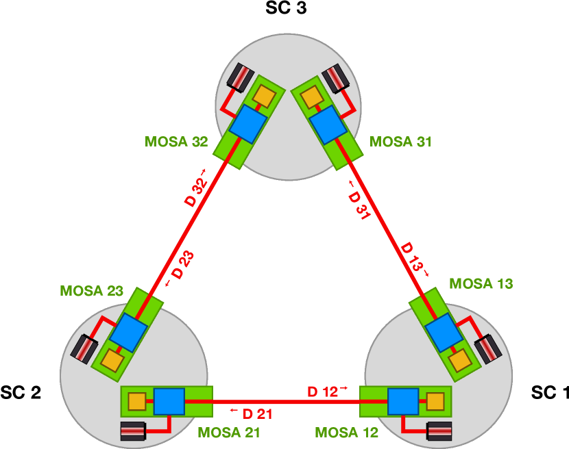
Figure 1: Standard LISA conventions. Spacecraft are labelled with 1, 2, 3; MOSAs are identified with two indices. Elements and quantities uniquely related to one spacecraft or one MOSA carry the same label.

The LISA measurements are labelled according to the MOSA on which they are performed. Light propagation times are indexed according to the MOSA on which they are measured, i.e., the receiving MOSA. In the rest of this paper, we only write quantities for a specific choice of indices (spacecraft or MOSA), and leave it to the reader to form all remaining expressions using circular permutation and swapping of indices.

The first step to computing the instrument response to the SGWB is to compute the deformation induced on the six LISA laser links via LISA GW Response. We use the linearity of the response function to write the overall response $y_{12}(t)$ of link $12$ as the discrete sum of the individual link responses to the $N$ point sources,

$$y_{12}(t)=\sum_{k=1}^{N}{y_{12,k}(t)}.$$ (7)

Similar equations can be written for all 6 LISA links.

The time series of frequency shifts $y_{12,k}(t)$, experienced by light traveling along link $12$, is computed by projecting the strain of point source $k$ on the link unit vector (computed from the spacecraft positions). The derivation of the link response, under usual approximations (expansion of the wave propagation time to first order, spacecraft immobile during this propagation time) can be found in Appendix A, as well as in the literature [e.g. 69]. It reads

$$y_{12,k}(t) \approx{}\frac{1}{2\quantity(1-\hat{\mathbf{k}}_{k}\dotproduct\hat{\mathbf{n}}_{12}(t))}\left[\right.$$

$$\left.H_{12,k}\quantity(t-\frac{L_{12}(t)}{c}-\frac{\hat{\mathbf{k}}_{k}\dotproduct\mathbf{x}_{2}(t)}{c})\right.$$

$$\left.-H_{12,k}\quantity(t-\frac{\hat{\mathbf{k}}_{k}\dotproduct\mathbf{x}_{1}(t)}{c})\right].$$ (8)

The $y_{ij}$ time series along the 6 LISA links are then combined in various ways to compute the TDI observables.

II.3 Instrumental noise

We include the dominant secondary noises in our analysis, which are test-mass acceleration noise and readout noise (mainly shot noise). We assume that laser frequency noise is perfectly suppressed by TDI, and therefore do not include it in our simulations.

We assume that the noises are uncorrelated in each MOSA, and identically distributed. The PSD of test-mass acceleration noise is given by

$$S_{\mathrm{TM}}(f)=a_{\mathrm{TM}}^{2}\left[1+\left(\frac{f_{1}}{f}\right)^{2}\right]\left[1+\left(\frac{f}{f_{2}}\right)^{4}\right],$$ (9)

where $a_{\mathrm{TM}}=3\times 10^{-15}\,\mathrm{ms^{-2}}$, $f_{1}=4\times 10^{-4}$ Hz and $f_{2}=8$ mHz. The readout noise PSD is

$$S_{\mathrm{OMS}}(f)=a_{\mathrm{OMS}}^{2}\left[1+\left(\frac{f_{3}}{f}\right)^{4}\right],$$ (10)

where $a_{\mathrm{OMS}}=15\times 10^{-12}\,\mathrm{mHz^{-1/2}}$ and $f_{3}=2$ mHz.

We generate instrumental noise directly at the science interferometer level, assuming no correlations between different interferometers. This way, only the diagonal elements of the links’ noise covariance matrix are non-vanishing. While unrealistic, this assumption is meant to simplify the subsequent analysis at relatively small cost in terms of impact on the noise covariance structure (see Section II.4).

II.4 Time-delay interferometry

TDI combinations are defined as linear combinations of time-shifted measurements. The first and second-generation Michelson combinations, $X_{1}$ and $X_{2}$, are given by [58],

$$\begin{split}X_{1}={}&y_{13}+\mathbf{D}_{13}y_{31}+\mathbf{D}_{131}y_{12}+\mathbf{D}_{1312}y_{21}\\ &-[y_{12}+\mathbf{D}_{12}y_{21}+\mathbf{D}_{121}y_{13}+\mathbf{D}_{1213}y_{31}],\end{split}$$ (11)

$$\begin{split}X_{2}={}&X_{1}+\mathbf{D}_{13121}y_{12}+\mathbf{D}_{131212}y_{21}+\mathbf{D}_{1312121}y_{13}+\mathbf{D}_{13121213}y_{31}\\ &-[\mathbf{D}_{12131}y_{13}+\mathbf{D}_{121313}y_{31}+\mathbf{D}_{1213131}y_{12}+\mathbf{D}_{12131312}y_{21}],\end{split}$$ (12)

Delay operators are defined by

$$\mathbf{D}_{ij}x(t)=x(t-L_{ij}(t)),$$ (13)

where $L_{ij}(t)$ is the delay time along link $ij$ at reception time $t$. Because light travel times evolve slowly with time, we compute chained delays as simple sums of delays rather than nested delays, i.e.,

$$\mathbf{D}_{i_{1},i_{2},\dots,i_{n}}x(t)=x\quantity(t-\sum_{k=1}^{n-1}{L_{i_{k}i_{k+1}}(t)}),$$ (14)

While this approximation cannot be used to study laser-noise suppression upstream of the LISA data analysis, it is sufficient when computing the response function. Note that these equations are left unchanged (up to a sign) by reflection symmetries. However, applying the three rotations generates the three Michelson combinations, $X,Y,Z$, for both generations. In our simulation, we compute them using the PyTDI [70] software.

Michelson combinations have highly-correlated noises. An quasi-uncorrelated set of TDI variables, $A,E,T$, can be obtained from linear combinations of $X,Y,Z$, given by [71]. However, $A,E,T$ are only exactly orthogonal (or uncorrelated) under the equal-armlength, equal noise assumptions. In this work, armlengths are not equal, so that we cannot consider $A,E,T$ as exactly uncorrelated. To visualize it, we compute their theoretical PSDs in Fig. 2, which shows that below 3 mHz the cross spectral density (CSD) levels (dashed curves) become dominant over the $TT$ PSD (solid brown curve).

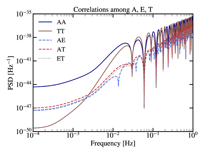
Figure 2: PSDs of TDI $A=E$ and $T$ (solid dark blue and brown lines, respectively) compared with their CSDs (light blue, red, and grey dashed lines).

Therefore, we perform the data analysis directly from TDI combinations $X,Y,Z$ by modelling their full $3\times 3$ covariance (see Section III).

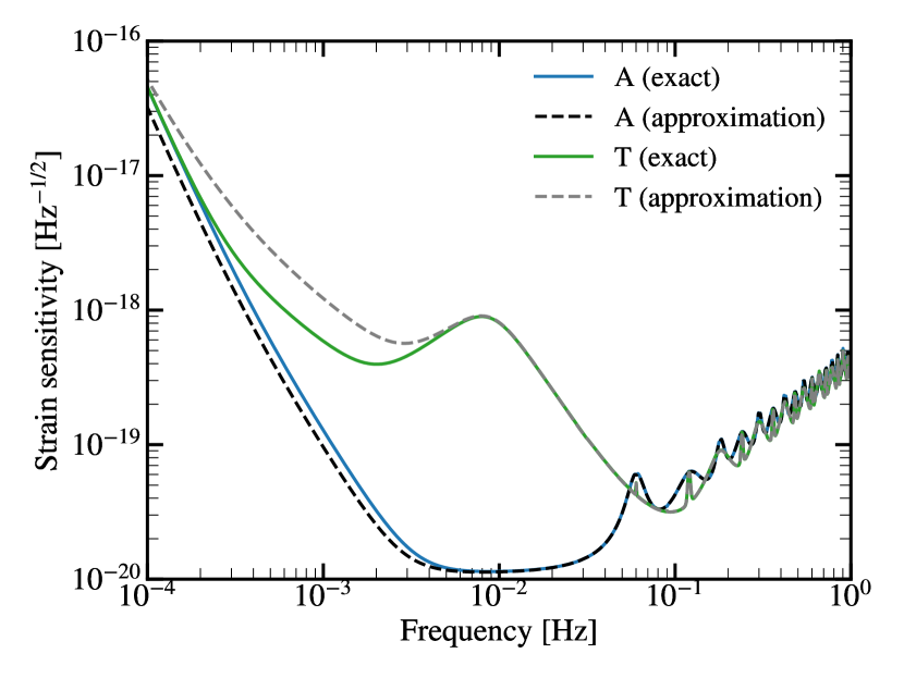
Figure 3: Effect of neglecting the cross-correlations among link measurements on the TDI sensitivity. The PSDs of TDI $A$ and $T$ with correlated links are represented by the continuous blue and green curves, respectively. The effect of assuming uncorrelated links is shown by the dashed black and gray lines. At high frequency (above 5 mHz), the difference is negligible. A deviation appears at low frequency, where the assumption leads to underestimating the strain noise level for both channels.

We illustrate in Fig. 3 the effect of the assumption we introduced in Section II.3 when neglecting the cross-correlations among the links $y_{ij}$, where we compare the change in GW sensitivity of TDI variables $A$ and $T$ with (solid curves) and without (dashed curves) the uncorrelated link assumption. While the relative error remains smaller than $5\text{\,}\mathrm{\char 37\relax}$ at high frequency, the plot shows a discrepancy of about $50\text{\,}\mathrm{\char 37\relax}$ in $A$ and a factor of 4 in $T$ at frequencies below 10 mHz. In other words, the assumption leads to a slight decrease of the overall noise level, and an overestimation of the attenuating power of $T$ at low frequency, which is usually considered as a quasi-null channel. However, the asymptotic behavior is the same: in the low-frequency limit, the $T$ channel is not suppressing gravitational waves better than $A$ or $E$.

III Data analysis model

In the analysis, we consider the data vector $\mathbf{\tilde{d}}\equiv(\tilde{X},\tilde{Y},\tilde{Z})^{T}$ of the Fourier-transformed TDI variables. For each frequency $f$, we encode the TDI transformation of Eq. 12 in a matrix $\mathbf{M}_{\mathrm{TDI}}$, so that can write the measured data $\mathbf{\tilde{d}}$ as a function of the link vector $\mathbf{\tilde{y}}$ as

$$\mathbf{\tilde{d}}(f)=\mathbf{M}_{\mathrm{TDI}}(f)\mathbf{\tilde{y}}(f),$$ (15)

where we defined the link vector as

$$\mathbf{\tilde{y}}=(\tilde{y}_{12},\,\tilde{y}_{23},\,\tilde{y}_{31},\,\tilde{y}_{13},\,\tilde{y}_{32},\,\tilde{y}_{21})^{T}.$$ (16)

To compute the transfer function $\mathbf{M}_{\mathrm{TDI}}(f)$, it is sufficient to approximate all the delays operators defined in Eq. 13 as complex phasing operators [72],

$$\mathbf{D}_{ij}\tilde{x}(f)\approx\tilde{x}(f)e^{-2\pi ifL_{ij}}.$$ (17)

We assume that the link data is only made of two stochastic processes: the SGWB signal $\mathbf{\tilde{y}}_{\mathrm{GW}}$ and the instrumental noise $\mathbf{\tilde{n}}$, so that

$$\mathbf{\tilde{y}}(f)=\mathbf{\tilde{y}}_{\mathrm{GW}}(f)+\mathbf{\tilde{n}}(f).$$ (18)

Since signal and noise are independent processes, the TDI data covariance can be written as the sum of the SGWB and instrumental noise link covariances,

$$\mathbf{C}_{y}(f)=\langle\mathbf{\tilde{y}}\mathbf{\tilde{y}}^{{\dagger}}\rangle=\mathbf{C}_{\mathrm{GW}}(f)+\mathbf{C}_{n}(f).$$ (19)

We straightforwardly deduce the TDI covariance from Eq. 15 as

$$\mathbf{C}_{d}(f)=\mathbf{M}_{\mathrm{TDI}}(f)\mathbf{C}_{y}(f)\mathbf{M}_{\mathrm{TDI}}^{{\dagger}}(f).$$ (20)

Note that it is not necessary to include laser frequency noise, as we assume that it is perfectly canceled by TDI. As discussed in Section II.3, we further assume that the noises affecting each link measurements are uncorrelated and all characterized by the same one-sided PSD $S_{n}(f)$. Therefore, their covariance is diagonal:

$$\mathbf{C}_{n}(f)\equiv\langle\mathbf{\tilde{n}}\mathbf{\tilde{n}}^{{\dagger}}\rangle=\frac{1}{2}S_{n}(f)\mathbf{I}_{6}.$$ (21)

This assumption allows us to easily express the contribution of the noise to the full covariance as a simple product

$$\mathbf{C}_{n}(f)=\frac{1}{2}S_{n}(f)\mathbf{M}_{\mathrm{TDI}}(f)\mathbf{M}_{\mathrm{TDI}}^{{\dagger}}(f).$$ (22)

As for the GW signal, we assume that it is isotropic and stationary, so that its response at any frequency $f$ and time $t_{0}$ can be encoded in a $6\times 6$ matrix $\mathbf{R}(f,t_{0})$ as

$$\mathbf{C}_{\mathrm{GW}}(f)=S_{h}(f)\mathbf{R}(f,t_{0}),$$ (23)

where the elements of $\mathbf{R}(f,t_{0})$ are explicitly derived in Appendix B. The background isotropy brings a quasi-independence on time, so that the choice of $t_{0}$ is irrelevant in our study.

The key point of the analysis is that we assume that we know both the frequency-dependent TDI transfer matrix $\mathbf{M}_{\mathrm{TDI}}(f)$ and the GW response matrix $\mathbf{R}(f,t_{0})$. Both of them depend on inter-spacecraft distances, which we suppose we know perfectly. Then, the parameters we have to estimate are the ones describing the signal PSD $S_{h}(f)$ and the noise PSD $S_{n}(f)$. Equation 4 provides the parametrization of $S_{h}(f)$, which includes the energy density $\Omega_{0}$ and spectral index $n$. The model for $S_{n}(f)$ is detailed in the next section.

III.1 Noise model

We aim at having a generic and flexible modeling of the noise. To this end, we model the single-link noise log-PSD with interpolating cubic B-spline functions. This basis provides a stable parametrization of any sufficiently smooth function, avoiding numerical errors that can arise when using high order polynomials. The parameters of the model are the logarithm of the control frequencies $x_{i}$ and their corresponding log-PSD ordinates $a_{i}$. We fix the first and last control frequencies to be the boundaries of the analysed frequency bandwidth, so that $x_{0}=\log f_{\min}$ and $x_{Q}=\log f_{\max}$, where $Q+1$ is the total number of control points. Then, we construct the spline function

$$\log S_{n}(f)=\sum_{i=1}^{Q+1}a_{i}B_{i,3}\left(\mathbf{\xi},f\right),$$ (24)

where $a_{i}$ are the spline coefficients and $\mathbf{\xi}$ is the vector of the $Q+5$ spline knots. The basis elements $B_{i,3}(\mathbf{\xi},f)$ are defined recursively as

$$B_{i,0}(f) =1,\textrm{ if $\xi_{i}\leq\log f<\xi_{i+1}$, otherwise $0$,}$$

$$B_{i,k}(f) =\frac{\log{f}-\xi_{i}}{\xi_{i+k}-\xi_{i}}B_{i,k-1}(f)+\frac{\xi_{i+k+1}-\log{f}}{\xi_{i+k+1}-\xi_{i+1}}B_{i+1,k-1}(f).$$ (25)

The spline knots are directly related to the control points as

$$\begin{split}\xi_{i}&=x_{0}\;\forall i\in[0,\,3];\\ \xi_{i+3}&=x_{i}\;\forall i\in[0,\,Q];\\ \xi_{i+3}&=x_{Q}\;\forall i\in[Q,\,Q+3];\\ \log S_{n}(e^{x_{i+3}})&=a_{i}\;\forall i\in[0,\,Q].\end{split}$$ (26)

In practice, we use the interp1d function of the SciPy package [73], which builds the spline basis based on the control log-frequencies $x_{i}$ and their corresponding ordinates $a_{i}$. Since the frequencies of the first and last control points are fixed, the spline model is described by $2Q$ parameters that we can gather in a vector $\boldsymbol{\theta}_{n}=(x_{0},\dots,x_{Q},a_{1},\dots,a_{Q-1})^{T}$.

III.2 Likelihood

In principle, one could directly write down the likelihood for the frequency-domain TDI data $\mathbf{\tilde{d}}$ using Whittle’s approximation [74]. To decrease the computational cost of the likelihood evaluation, we instead consider frequency sample averages of the periodogram.

Let us define the normalized windowed discrete Fourier transform (DFT) of any multivariate time series of length $N_{x}=\lfloor Tf_{s}\rfloor$ as

$$\mathbf{\tilde{x}}(f_{k})=\sqrt{\frac{2}{\kappa_{2}f_{s}}}\sum_{n=0}^{N_{x}-1}w_{n}\mathbf{x}_{n}e^{-2\pi kn/N_{x}},$$ (27)

where $w_{n}$ is a time window smoothly decreasing to zero at the edges of the time series, and $\kappa_{p}=\sum_{n=0}^{N_{x}-1}{w_{n}}^{p}$. We choose this normalization such that the periodogram is directly given by the square modulus of $\tilde{\mathbf{x}}_{k}$, and its expectation is directly comparable with the one-sided PSD.

At each frequency bin $f_{k}$, we define the $3\times 3$ periodogram matrix as $\mathbf{P}(f_{k})\equiv\mathbf{\tilde{d}}(f_{k})\mathbf{\tilde{d}}(f_{k})^{{\dagger}}$. To compress the data, we split the frequency series $\mathbf{\tilde{d}}$ into $J$ consecutive, non-overlapping segments. We call $f_{j}$ the central frequency and $n_{j}$ the size of each segment $j$. We define the averaged periodogram matrix $\mathbf{\bar{P}}(f_{j})$ by averaging the periodograms over the frequency bins within each segment $j$,

$$\mathbf{\bar{P}}(f_{j})\equiv\frac{1}{n_{j}}\sum_{k=j-\frac{n_{j}}{2}}^{j+\frac{n_{j}}{2}}\mathbf{\tilde{d}}(f_{k})\mathbf{\tilde{d}}(f_{k})^{{\dagger}}.$$ (28)

If the DFTs $\mathbf{\tilde{d}}(f_{k})$ were uncorrelated between different frequency bins, the matrix $\mathbf{Y}(f_{j})\equiv\nu(f_{j})\mathbf{P}(f_{j})$ would follow a complex Wishart distribution with $\nu(f_{j})=n_{j}$ degrees of freedoms (DoFs) and scale matrix $\mathbf{C}_{d}(f)$, with a probability density function

$$p({\mathbf{Y}(f)}|\boldsymbol{\theta})=\frac{\quantity|\mathbf{Y}(f)|^{\nu-3}\operatorname{exp}\quantity[-\operatorname{tr}(\mathbf{C}_{d}^{-1}\mathbf{Y}(f))]}{\quantity|\mathbf{C}_{d}(f)|^{\nu}\cdot\mathcal{C}\tilde{\Gamma}_{3}(\nu)},$$ (29)

where $\mathcal{C}\tilde{\Gamma}_{p}(\nu)$ is the complex gamma function, $\operatorname{tr\left(\cdot\right)}$ is the trace operator and $\quantity|\mathbf{A}|$ is the determinant of any matrix $\mathbf{A}$. In reality, the frequency bins that are close to each other are mildly correlated, depending on the choice of the window function $w_{n}$ in Eq. 27. As a result, the effective number of DoFs $\nu(f_{j})$ is smaller than the number of averaged frequency bins $n_{j}$. A good measure of the reduction factor is provided by the normalized equivalent noise bandwidth $N_{\mathrm{bw}}$, defined for any window $w$ and time series size $N_{d}$ as

$$N_{\mathrm{bw}}=N_{d}\frac{\kappa_{2}}{\kappa_{1}},$$ (30)

which is expressed in number of frequency bins. Values of $N_{\mathrm{bw}}$ for various windows can be found in [75]. The effective number of DoFs is then given by $\nu(f_{j})=n_{j}/N_{\mathrm{bw}}$.

Taking the logarithm of Eq. 29 above and keeping only the terms depending on the parameters $\boldsymbol{\theta}$ yields

$$\log p({\mathbf{Y}(f)}|\boldsymbol{\theta})=-\operatorname{tr}(\mathbf{C}_{d}^{-1}\mathbf{Y}(f))-\nu(f)\log\quantity|\mathbf{C}_{d}(f)|.$$ (31)

The full log-likelihood across the analyzed bandwidth is then the sum over all frequency bins

$$\mathcal{L}_{\mathbf{Y}}(\boldsymbol{\theta})=\sum_{j=0}^{J-1}\log p({\mathbf{Y}(f_{j})}|\boldsymbol{\theta}).$$ (32)

When both noise and signal are included in the likelihood, the vector of model parameters $\boldsymbol{\theta}$ includes the control point locations, the spline coefficients, and the GW parameters $\boldsymbol{\theta}=(x_{0},\ldots,x_{Q},a_{1},\ldots,a_{Q-1},\log\Omega_{0},n)^{T}$.

III.3 Priors

Aiming at a robust analysis, we choose poorly constraining priors for the noise parameters. We let the control points take value in an interval bounded by one order of magnitude below and above the true noise model $S_{n,\mathrm{true}}$ (which is used for the injection). This way, we have

$$S_{n}(f)\in\left[10^{-1}\,S_{n,\mathrm{true}}(f);\;10\,S_{n,\mathrm{true}}(f)\right].$$ (33)

Note that this prior does not reflect the allocated margins for the required LISA sensitivity, but enables us to remain conservative in our analysis.

We allow the control frequencies to take value within the analyzed bandwidth $\left[f_{\mathrm{min}},f_{\mathrm{max}}\right]$. To enforce a relatively even distribution of the control points, we assign to each of them a Beta distribution conditioned on the location of the previous one, such that

$$p\left(x_{i}|x_{i-1}\right)\propto u_{i}^{\alpha_{i}-1}(1-u_{i})^{\beta_{i}-1},$$ (34)

where $u_{i}\equiv\left(x_{i}-x_{i-1}\right)/\left(x_{Q}-x_{i-1}\right)$ is the position of control point $x_{i}$ relative to the previous one $x_{i-1}$, rescaled in the interval $[0,\,1]$. We choose parameters values $\alpha_{i}=2$ and $\beta_{i}=Q-i+2$ so that the mode of the conditional distribution peaks at $(x_{Q}-x_{i-1})/(Q-i)$. This choice ensures that if the control point $x_{i-1}$ is given, as there are $Q-i$ control points left to be placed, the next one has more probability to be placed in the first $1/(Q-i)\mathrm{{}^{th}}$ of the remaining frequency band.

Concerning the SGWB parameters, we impose uniform priors on $\log\Omega_{0}$ and on $n$, respectively in intervals $[-35,\,-28]$ and $[-5,7]$.

IV Detection and parameter estimation

IV.1 Detection

In a Bayesian framework, detecting the presence of a stochastic process can be done through model comparison: one model assumes that the data only contains noise (null hypothesis $H_{0}$), while the other model assumes the presence of a SGWB in addition to the noise (tested hypothesis $H_{1}$). We compare the models by computing their Bayes factor, defined as the ratio of their evidences. The log-Bayes factor is then

$$\log\mathcal{B}_{10}(\mathbf{Y})=\log Z_{1}(\mathbf{Y})-\log Z_{0}(\mathbf{Y}),$$ (35)

where $Z_{i}(y)\equiv\int_{{\boldsymbol{\theta}}_{i}}p\left(y|H_{i}\right)d\boldsymbol{\theta}$ is the evidence of the model under hypothesis $H_{i}$ and $\Theta_{i}$ is the space in which $\boldsymbol{\theta}_{i}$ is allowed to take values. The presence of a SGWB is claimed when the Bayes factor stands above a given threshold.

When dealing with parallel-tempered Markov chain Monte Carlo (MCMC) outputs, we can approximate the evidence by thermodynamic integration [76],

$$\log Z_{i}(\mathbf{Y})=\int_{0}^{1}\mathrm{E}_{\beta}\quantity[\log p\left(\mathbf{Y}|\boldsymbol{\theta},H_{i}\right)]\differential{\beta},$$ (36)

where the expectation $\mathrm{E}_{\beta}$ is taken with respect to the tempered posterior density $p_{\beta}\left(\mathbf{Y}|\boldsymbol{\theta},H_{i}\right)\propto p\left(\mathbf{Y}|\boldsymbol{\theta},H_{i}\right)^{\beta}p(\boldsymbol{\theta},H_{i})$. The variable $\beta$ is the inverse temperature of the tempered chain, and $\mathrm{E}_{\beta}$ is the expectation of the chain at temperature $1/\beta$ taken over the parameter space $\Theta$.

IV.2 Averaged Bayes factors

We aim to find the parameter pairs $(\Omega_{0},n)$ for which the Bayes factor is equal to the detection threshold $\mathcal{B}_{\mathrm{thresh}}$. To do that, we compute the posterior distributions under both $H_{0}$ and $H_{1}$ for a wide range of parameter values. The Bayes factor depends on the specific data realization; instead of generating hundreds of data realizations for each parameter pair, we choose to consider the averaged Bayes factor, that we define as the Bayes factor computed from the expected likelihood under the true distribution when $H_{1}$ is true.

In other words, if the data is described by the true parameter vector $\boldsymbol{\theta}^{\star}$, then we can compute the averaged log-Bayes factor

$$\overline{\log\mathcal{B}_{10}}=\log\mathcal{B}_{10}(\mathbf{\bar{Y}}),$$ (37)

where $\mathbf{\bar{Y}}=\operatorname{E}_{\theta^{\star}}[\mathbf{Y}]$ is the expectation of the data $\mathbf{Y}$ under the true hypothesis. Note that $\overline{\log\mathcal{B}_{10}}$ is not the statistical expectation of the log-Bayes factor, but we will show later that using $\overline{\log\mathcal{B}_{10}}=\mathcal{B}_{\mathrm{thresh}}$ provides a conservative criterion for detection.

IV.3 Optimal model order

For this work, we adopted a spline model that is flexible enough to fit the spectral series. With the right parametrization, it yields satisfactory results in inferring the instrumental noise PSD shape (see Section IV.4). One of the challenges of this strategy is to choose the most suitable model order, i.e., the optimal number of spline knots. This is crucial for avoiding over-fitting situations, but also biases in the search and in parameter estimation.

As described previously, we perform a model selection by computing Bayes factors between two hypotheses. Thus, for a given data scenario, we can either perform the analysis multiple times with different spline orders, or dynamically estimate the model order together with its corresponding parameters. As a cross-validation test for our analyses here, we choose the latter applied on a simplified case. We use a reversible jump (RJ)-MCMC algorithm [77], which is generalization of the Metropolis-Hastings [78, 79, 80] algorithm, capable of searching in parameter spaces of varying dimensionality (see [81] for a review of sampling techniques). In particular, we use a RJ algorithm enhanced with parallel tempering techniques [82, 83, 84] to efficiently identify the optimal number of knots in our spline model.

To simplify the procedure, we focus on instrumental noise only. We simulate one year of noise data, as described in Section II, without any GW signal present. We then build a likelihood function that is computationally efficient.

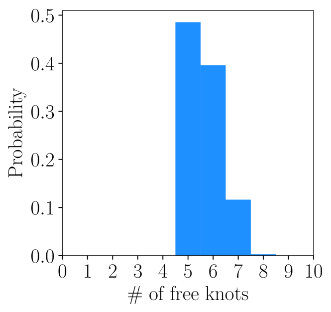
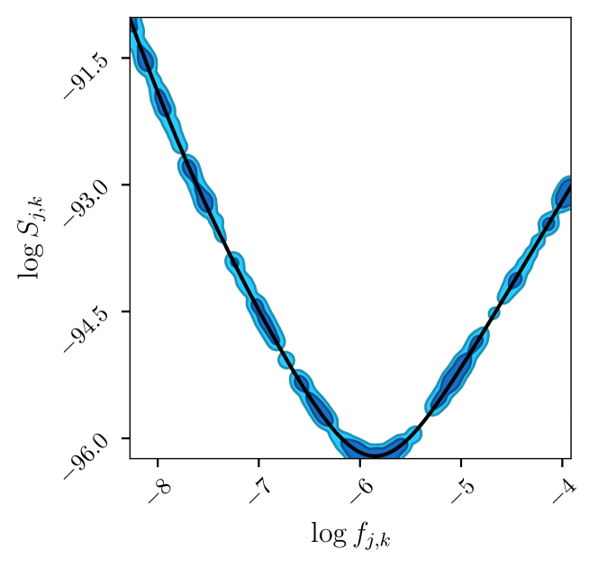
Figure 4: Estimating the optimal model order using RJ-MCMC. In this investigation, we have fixed the frequencies of the two edge knots, while letting the algorithm determine the optimal number of internal knots, together with their frequencies and amplitude. Right: posterior samples of the knots amplitudes $\log S_{j,k}$ and frequencies $\log f_{j,k}$ for all given spline models of order $k$, as sampled with our RJ algorithm (we stack the chains for all $k$). The algorithm explores the true noise curve (solid black line) by proposing spline knots positioned across the frequency range (see main text for more details). The plot was generated with [85].

Our spline model fixes the control frequencies of the two knots at the edges of our spectrum; their amplitudes $S_{\mathrm{low}}$ and $S_{\mathrm{high}}$ are left as free parameters to be estimated. The number of other knots $k$, their frequencies $S_{j,k}$ and amplitudes $f_{j,k}$ in-between are also determined from the data. We remind here that the $j$ index corresponds to the spline number for the given model order $k$.

For the knot parameters, we have chosen a quite broad uniform prior, $\log S_{j,k}\sim\mathcal{U}[-100,\,-91]$ and for $\log f_{j,k}$, a uniform prior across the log-frequency range; for the spline model order $k$, we used an uninformative prior $k\sim\mathcal{U}[3,\,30]$. Running the algorithm for 10 temperatures [82] with 20 walkers each [83] yields the result shown in the left panel of Fig. 4.

It is particularly interesting to also inspect the 2D posterior slices of the parameters, shown in the right panel of Fig. 4. We have essentially sampled the full parameter space of $\log S_{j,k}$ and $\log f_{j,k}$ for all the possible values of the dimensionality $k$ of the model. The figure shows that there is no unique solution when fitting both the frequencies and amplitudes of the spline knots, and the MCMC chains explore the true shape of the noise spectra.

From the posterior distribution of the model order $k$, shown in the left panel of Fig. 4, we see that a maximum can be found between $k=5$ and $k=6$. In the rest of the study, we fix the model order to this optimal value $k=5$, i.e. $5+2$ knots. This translates to twelve parameters (the internal knots’ frequencies and amplitudes, plus the frequencies of the two edge knots).

IV.4 Assessment of the detectability of a stochastic gravitational-wave background

Now we compute the averaged Bayes factors for a wide range of SGWB parameters to assess our ability to detect a SGWB with a noise of unknown spectral shape, under the assumptions that we stated in Section III. For a set of spectral indices ranging from -4 to 5, and log-energy densities between ${10}^{-14}$ and ${10}^{-12}$, we run our Bayesian model comparison and plot the results in Fig. 5.

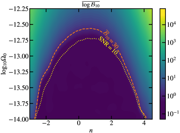
Figure 5: Left: averaged log-Bayes factor contour plot for a range of SGWB spectral index $n$ ($x$-axis) and log-energy density $\log\Omega_{0}$ ($y$-axis) with a knee frequency of $f_{0}=$3.16\text{\,}\mathrm{mHz}$$. The color map represents the values of the decimal logarithm of Bayes factor, with warmer shades indicating larger values. The orange dashed line is the detection threshold taken equal to 30, considered as a strong evidence for the presence of the SGWB. The yellow dotted line shows the SNR-10 line as a comparison.

We represent values of log-Bayes factors using a color scale, with warmer colors signify large detection evidences. From the initial set of 272 computed point, we interpolate the log-Bayes factor values on a finer grid of $100\times 100$ points using a Gaussian process regression. This allows us to plot a line of constant Bayes factor (dashed orange) of $\overline{\mathcal{B}_{10}}=30$, which is considered as a detection threshold for strong evidence for hypothesis $H_{1}$ [38]. All couples of parameters that lie below this line are considered as undetectable signals, and all above values are strong detections. For example, we find that the amplitude detection threshold for a scale-invariant SGWB ($n=0$) is about $\Omega_{0}=$2.5\text{\times}{10}^{-13}$$, which is close to what previous work using a parametrized noise PSDs model found (for example, Adams and Cornish get $\Omega_{0}=$1.7\text{\times}{10}^{-13}$$). Besides the obvious effect of the increase of detectability with the energy density, we also observe a dependence that is strongly tied to the spectral shape of the noise present in the data. For a given energy density, the Bayes factor is minimum when $n$ is between 0.5 and 1. We observe the same minimum for the SNR curve, suggesting that our ability to detect the signal is mainly driven by its SNR, which is itself determined by both $\Omega_{0}$ and $n$.

The location of the SNR minimum is set by the strain sensitivity curve in Fig. 3, as well as the SGWB strain PSD’s dependence on frequency, which is proportional to $f^{n-3}$, as shown in Eq. 6. Note that the choice of the knee frequency (of about $3\text{\,}\mathrm{mHz}$) also drives the location of the minimum through its contribution to the effective SGWB amplitude.

Figure 5 provides us with the range of power-law parameters that LISA will be able to probe. This result can be considered in the context of previous measurements. The LIGO, Virgo and KAGRA collaborations are able to put upper limits on the isotropic gravitational-wave background from Advanced LIGO’s and Advanced Virgo’s third observing run [16]. In particular, they find that the dimensionless energy density is bounded as $\Omega_{\mathrm{GW}}\leq$5.8\text{\times}{10}^{-9}$$ at the $95\text{\,}\mathrm{\char 37\relax}$ credible level for a frequency-independent gravitational-wave background, with $99\text{\,}\mathrm{\char 37\relax}$ of the sensitivity coming from the band $20\text{\,}\mathrm{Hz}76.6\text{\,}\mathrm{Hz}$. They also find the upper limit $\Omega_{\mathrm{GW}}\leq$3.4\text{\times}{10}^{-9}$$ at $25\text{\,}\mathrm{Hz}$ for a power-law gravitational-wave background with a spectral index of 2/3 in the band $20\text{\,}\mathrm{Hz}90.6\text{\,}\mathrm{Hz}$, and $\Omega_{\mathrm{GW}}\leq$3.9\text{\times}{10}^{-10}$$ at $25\text{\,}\mathrm{Hz}$ for a spectral index of 3, in the band $20\text{\,}\mathrm{Hz}291.6\text{\,}\mathrm{Hz}$.

The NANOGrav collaboration [22], using their $12.5\text{\,}\mathrm{yr}$ pulsar-timing data set, finds that under their fiducial model, the Bayesian posterior of the amplitude has median $1.92^{+0.75}_{-0.55}\times 10^{-15}$ for an $f^{-2/3}$ spectrum (as expected from a population of inspiralling supermassive black holes) at a reference frequency of $1\text{\,}{\mathrm{yr}}^{-1}$. The International Pulsar Timing Array (IPTA) collaboration [24], using their second data release and for a spectral index of $-2/3$, finds a recovered amplitude of $2.8^{+1.2}_{-0.8}\times 10^{-15}$ at a reference frequency of $1\text{\,}{\mathrm{yr}}^{-1}$.

We gather these experimental measurements in Table 1 and compare them to what LISA could observe, should the frequency dependence of the GW background remain constant in-between the detectors sensitive bands. This comparison shows that LISA would be able to detect, or place tighter constraints, on energy densities for SGWB searched in LIGO-Virgo or pulsar timing array data. Besides, the detection limits of about ${10}^{-14}$ we obtain in Fig. 5 for extreme spectral indices like $n=-3$ or $n=4$ would yield huge amplitudes in the IPTA and LIGO-Virgo bands, respectively. Those lying well above the detectors sensitivity, such power laws would be visible today and are therefore not expected to arise in LISA.

Detector	$n$	$\Omega_{\mathrm{det}}(f_{\mathrm{det}})$	$\Omega_{\mathrm{LISA}}(f_{0})$	Thresh.	Refs
LVK	$0$	$5.8\cdot 10^{-9}$	$5.8\cdot 10^{-9}$	$2.5\cdot 10^{-13}$	[16]
LVK	$2/3$	$3.4\cdot 10^{-9}$	$8.3\cdot 10^{-12}$	$2.7\cdot 10^{-13}$	[16]
NANOGrav	$-2/3$	$1.9\cdot 10^{-15}$	$9.2\cdot 10^{-9}$	$2.0\cdot 10^{-13}$	[22]
IPTA	$-2/3$	$2.8\cdot 10^{-15}$	$1.3\cdot 10^{-8}$	$2.0\cdot 10^{-13}$	[24]

Table 1: Comparison of LISA capabilities with current detector constraints on SGWB parameters. The columns from left to right show, respectively, the detector’s collaboration name; the power-law index value; the energy density computed at the detector pivot frequency $f_{\text{det}}$ ($25\text{\,}\mathrm{Hz}$ for LVK, $1\text{\,}{\mathrm{yr}}^{-1}$ for NANOGrav and IPTA); the extrapolated energy density at LISA’s $3\text{\,}\mathrm{mHz}$ pivot frequency; the detection threshold computed in this study; and the reference from which we extract the constraints.

IV.5 Parameter estimation

As an example of parameter posterior, we pick the case $\Omega_{0}=$1.63\text{\times}{10}^{-13}$$ and $n=-1$. It is particularly interesting because it lies in the detection limit and also features a SGWB strain PSD slope of $-4$, which is similar to the low-frequency shape of the strain sensitivity curve (in power). We plot the signal parameters’ joint posterior in Fig. 7 and verify that the injected values lies within the credible interval. We also compute the corresponding TDI signal and noise PSDs from posterior samples in Fig. 6. The maximum a posteriori estimate (MAP) of the GW signal parameters yields the red solid curve, which is close to the true PSD shown by the dashed purple curve, even though the credible interval is relatively large. The noise PSD represented by the blue curve is better constrained as it dominates over the signal in the entire frequency band. This is confirmed by the spline reconstruction of the links’ noise PSD in Fig. 8, where the MAP estimate (in blue) coincides with the true PSD (dashed orange) with a relative error smaller than $10\text{\,}\mathrm{\char 37\relax}$ in most of the analyzed frequency band.

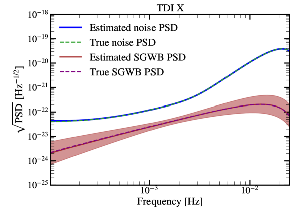
Figure 6: Posteriors of the noise (blue) and the SGWB (red) PSDs in TDI channel $X$ for an injection with $\Omega_{0}=$1\text{\times}{10}^{-13}$$ and $n=-1$. The light red-shaded area represents the 3-$\sigma$ credible interval.

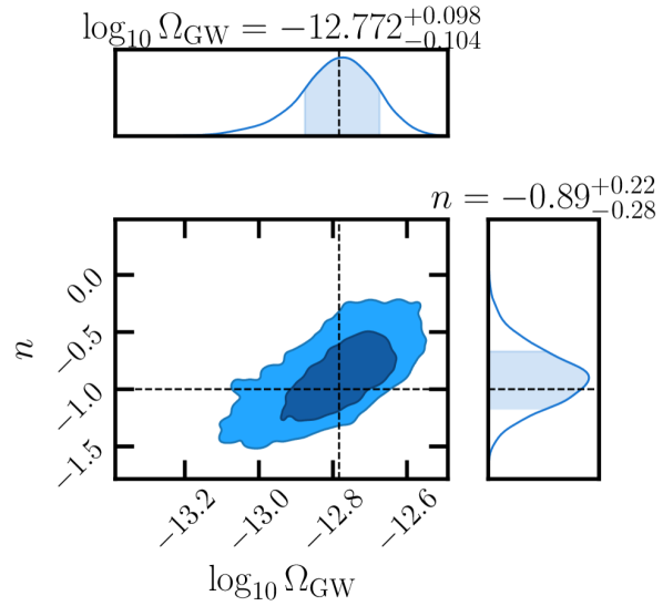
Figure 7: Posteriors of the SGWB parameters (log-energy density and power-law index) for an injection of $\Omega_{0}=$1.63\text{\times}{10}^{-13}$$ and $n=-1$.

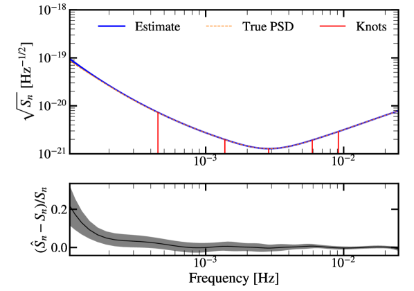
Figure 8: Upper panel: posterior of the single-link noise PSD (blue) compared to the true value (dashed orange). The vertical red lines locate spline control points. Bottom panel: average relative error obtained with the MAP estimate, along with the 3-$\sigma$ credible interval.

IV.6 Validity of the averaged Bayes factors

In this section, we check that the averaged Bayes factor $\overline{\log\mathcal{B}_{10}}$ we compute with the method outlined in Section IV.1 is consistent with what we obtain with single data realizations. We generate simulated datasets following the model described in Section II; we include different realizations of both the noises and the SGWB for a handful of cases.

As we are particularly interested in LISA’s ability to detect a SGWB as a function of its shape, we extract the pairs of parameters defining the contour line $\overline{\mathcal{B}_{10}}(\Omega_{0},n)=30$ corresponding to the detection threshold (dashed orange line in Fig. 5). For each of these pairs corresponding to an integer power law index between $n=-2$ and $n=3$, we generate 10 data realizations under hypothesis $H_{1}$, from which we sample the posterior distributions and compute the evidences under both $H_{0}$ and $H_{1}$. We plot the histogram of the log-Bayes factors we obtain in Fig. 9 (orange), along with the detection threshold line (dashed red). The distribution we obtain exhibits a significant variance, but the mean is located towards Bayes factor values larger than the threshold. Among the Bayes factors estimated from these simulations, $80\text{\,}\mathrm{\char 37\relax}$ yield a value above the detection threshold.

In addition, we perform a similar analysis with 30 data realizations generated under hypothesis $H_{0}$ (containing only noise), and plot the histogram of the log-Bayes factors we obtain in blue on the same figure. They are concentrated around zero and distributed approximately like a chi-squared distribution. All the simulations produce values below the detection threshold, i.e., there are no false positive for these data realizations. The orange and blue distributions show that our derivation of detection limit is a conservative one as it minimizes the false-alarm rate at the expense of $20\text{\,}\mathrm{\char 37\relax}$ of false negatives.

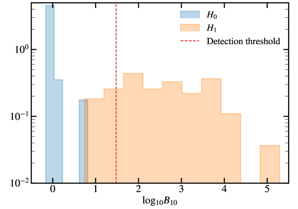
Figure 9: Statistics of the decimal log-Bayes factor for couples of parameters $(\log\Omega_{0},n)$ corresponding to the detection threshold $\mathcal{B}_{10}=30$ (vertical red dashed line) derived from the contour plot in Fig. 5. For each power-law index, Bayes factors are computed for 10 data realizations under $H_{1}$ (noise and signal, in blue). The histogram of log-Bayes factors computed for 20 data realizations under $H_{0}$ (noise only) is also shown in orange.

V Conclusion

We have presented a method to detect SGWBs from LISA measurements, which, for the first time, is model-agnostic with respect to the instrumental noise spectral shape. Instead, we use a flexible model for the single-link noise PSDs based on cubic splines. Such modelling could avoid biasing the instrument characterization and the subsequent impact on the signal detection. We test for the presence of an isotropic SGWB through Bayesian model comparison, where we model both the signal and the noise transfer functions. We also adopt a template-based search to look for power-law signals. As a step towards more realistic instrumental setup compared to previous studies, we simulate interferometric data in the time domain, featuring a spacecraft constellation with unequal, time-varying armlengths. In this configuration, the assumptions underlying classic pseudo-orthogonal TDI variables $A,E,T$ break down. Therefore, we directly analyze the three second-generation Michelson variables $X_{2}$, $Y_{2}$, $Z_{2}$ and account for their full frequency-dependent covariance matrix. We restrict the observation time to one year and the analyzed frequency bandwidth to the interval $0.1\text{\,}\mathrm{mHz}50\text{\,}\mathrm{mHz}$ to mitigate computation time and artefacts related to blind frequency spots of LISA’s sensitivity.

We run multiple injections of SGWBs with a wide range of energy densities and power-law spectral indices to determine the region of the parameter space that would allow for a detection. We confirm LISA’s ability to detect a scale-invariant SGWB with an energy density above $\sim$2\text{\times}{10}^{-13}$$, a threshold that was previously reported in the literature, in spite of the added flexibility on the noise modeling. This confirms LISA’s ability to detect SGWBs that not accessible to today’s GW detectors. In addition, we show that with a pivot frequency of $f_{0}\sim$3\text{\,}\mathrm{mHz}$$ and power-law indices ranging between $n=-2$ and $n=3$, we can distinguish GW backgrounds from noise provided that their SNR is sufficiently large. We also probe larger absolute values of indices, keeping in mind that such extreme cases are unlikely to correspond to any signal as they would have been detected by current observatories.

This work motivates further investigations to improve the robustness of SGWBs searches with space-based observatories against instrumental noise modeling. In this perspective, future works will account for distinct transfer functions for the different noise sources, and in particular for acceleration and readout noises. We also plan to allow for different noise levels across the various interferometers. Moreover, we performed our study based on a power-law model of isotropic stochastic signals, which does not reflect the full diversity of processes that can lead to stochastic backgrounds of GWs. We plan to test other templates, but also to assess to what extent one can be agnostic with respect to both the signal and noise shapes while preserving the ability to tell them apart. As a final step, we aim to include the various astrophysical stochastic signals in our analysis, thus testing this pipeline to the greater LISA global fit scheme [64].

Appendix A Derivation of the time-domain response function

We express each stochastic point source’s position using the Cartesian coordinate system $(\mathbf{x},\mathbf{y},\mathbf{z})$, defined such that $(\mathbf{x},\mathbf{y})$ is the plane of the ecliptic. We introduce the associated spherical coordinates $(\theta,\phi)$, based on the orthonormal basis vectors $(\hat{\mathbf{e}}_{r},\hat{\mathbf{e}}_{\theta},\hat{\mathbf{e}}_{\phi})$, as illustrated in Fig. 10. The $k$-th source localization is parametrized by the ecliptic latitude $\beta_{k}=\pi/2-\theta_{k}$ and the ecliptic longitude $\lambda_{k}=\phi_{k}$. The basis vectors read

$$\hat{\mathbf{e}}_{r,k} =(\cos\beta_{k}\cos\lambda_{k},\cos\beta_{k}\sin\lambda_{k},\sin\beta_{k}),$$ (38a)

$$\hat{\mathbf{e}}_{\theta,k} =(\sin\beta_{k}\cos\lambda_{k},\sin\beta_{k}\sin\lambda_{k},-\cos\beta_{k}),$$ (38b)

$$\hat{\mathbf{e}}_{\phi,k} =(-\sin\lambda_{k},\cos\lambda_{k},0).$$ (38c)

Figure 10: Parametrization of the localization for point source $k$. The propagation vector is $\mathbf{\hat{k}_{k}}$, and the polarization vectors are $\mathbf{\hat{u}_{k}}$ and $\mathbf{\hat{v}_{k}}$. Adapted from the LDC Manual, available at https://lisa-ldc.lal.in2p3.fr.

The propagation vector is $\hat{\mathbf{k}}_{k}=-\hat{\mathbf{e}}_{r,k}$. We define the polarization vectors as $\hat{\mathbf{u}}_{k}=-\hat{\mathbf{e}}_{\phi,k}$ and $\hat{\mathbf{v}}_{k}=-\hat{\mathbf{e}}_{\theta,k}$. This produces, for source $k$, a direct orthonormal basis $(\hat{\mathbf{u}}_{k},\hat{\mathbf{v}}_{k},\hat{\mathbf{k}}_{k})$.

The time series of frequency shifts $y_{12,k}(t)$, experienced by light traveling along link $12$, is computed by projecting the strain of point source $k$ on the link unit vector $\hat{\mathbf{n}}_{12}$ (computed from the spacecraft positions),

$$\begin{split}H_{12,k}(t)={}&h_{+}(t,\hat{\mathbf{n}}_{k})\xi_{+}(\hat{\mathbf{u}}_{k},\hat{\mathbf{v}}_{k},\hat{\mathbf{n}}_{12})\\ &+h_{\times}(t,\hat{\mathbf{n}}_{k})\xi_{\times}(\hat{\mathbf{u}}_{k},\hat{\mathbf{v}}_{k},\hat{\mathbf{n}}_{12}),\end{split}$$ (39)

where we assume that the link unit vector $\hat{\mathbf{n}}_{12}$ is constant during the light travel time. The antenna pattern functions are given by

$$\xi_{+}(\hat{\mathbf{u}}_{k},\hat{\mathbf{v}}_{k},\hat{\mathbf{n}}_{12}) =\quantity(\hat{\mathbf{u}}_{k}\dotproduct\hat{\mathbf{n}}_{12})^{2}-\quantity(\hat{\mathbf{v}}_{k}\dotproduct\hat{\mathbf{n}}_{12})^{2},$$ (40a)

$$\xi_{\times}(\hat{\mathbf{u}}_{k},\hat{\mathbf{v}}_{k},\hat{\mathbf{n}}_{12}) =2\quantity(\hat{\mathbf{u}}_{k}\dotproduct\hat{\mathbf{n}}_{12})\quantity(\hat{\mathbf{v}}_{k}\dotproduct\hat{\mathbf{n}}_{12}).$$ (40b)

Light emitted by spacecraft 2 at $t_{2}$ reaches spacecraft 1 at $t_{1}$. Accounting for the effect of source $k$ only, these two times $t_{1}$ and $t_{2}$ are related by $H_{12,k}(\mathbf{x},t)$,

$$t_{1}\approx t_{2}+\frac{L_{12}}{c}-\frac{1}{2c}\int_{0}^{L_{12}}{H_{12,k}(\mathbf{x}(\lambda),t(\lambda))\differential{\lambda}},$$ (41)

We approximate the wave propagation time to first order as $t(\lambda)\approx t_{2}+\lambda/c$. Also, $\mathbf{x}(\lambda)=\mathbf{x}_{2}(t_{2})+\lambda\hat{\mathbf{n}}_{12}(t_{2})$, where $\mathbf{x}_{2}(t_{2})$ represents the position of the emitter spacecraft at emission time. Using these two expressions, we can further refine $H_{12,k}$ as

$$\begin{split}&H_{12,k}\quantity(\mathbf{x}(\lambda),t(\lambda))=H_{12,k}\quantity(t(\lambda)-\frac{\hat{\mathbf{k}}_{k}\dotproduct\mathbf{x}(\lambda)}{c})\\ &=H_{12}\quantity(t_{2}-\frac{\hat{\mathbf{k}}_{k}\dotproduct\mathbf{x}_{2}(t_{2})}{c}+\frac{1-\hat{\mathbf{k}}_{k}\dotproduct\hat{\mathbf{n}}_{12}(t_{2})}{c}\lambda),\end{split}$$ (42)

Combining Eqs. 42 and 41 and differentiating the resulting expression with respect to $t_{2}$ yields the relative frequency shift, $y_{12}$, experienced by light as it travels along link 12,

$$y_{12,k}(t_{2}) \approx\frac{1}{2\quantity(1-\hat{\mathbf{k}}_{k}\dotproduct\hat{\mathbf{n}}_{12}(t_{2}))}$$

$$\left[H_{12,k}\quantity(t_{2}-\frac{\hat{\mathbf{k}}_{k}\dotproduct\mathbf{x}_{2}(t_{2})}{c})\right.$$

$$\left.-H_{12,k}\quantity(t_{2}-\frac{\hat{\mathbf{k}}_{k}\dotproduct\mathbf{x}_{1}(t_{1})}{c}+\frac{L_{12}}{c})\right].$$ (43)

Here, we have introduced the receiver spacecraft position at reception time $\mathbf{x}_{1}(t_{1})=\mathbf{x}_{2}(t_{2})+L_{12}\hat{\mathbf{n}}_{12}(t_{2})$. These spacecraft positions are expressed in the coordinate frame introduced represented Fig. 10, and computed with LISA Orbits [86].

Using $t_{1}\approx t_{2}+L_{12}/c$ and the fact that the spacecraft moves slowly compared to the propagation timescale, we obtain $\mathbf{x}_{2}(t_{2})\approx\mathbf{x}_{2}(t_{1})$ and $\hat{\mathbf{n}}_{12}(t_{1})\approx\hat{\mathbf{n}}_{12}(t_{2})$,

$$y_{12,k}(t_{1}) \approx\frac{1}{2\quantity(1-\hat{\mathbf{k}}_{k}\dotproduct\hat{\mathbf{n}}_{12}(t_{1}))}$$

$$\left[H_{12,k}\quantity(t_{1}-\frac{L_{12}(t_{1})}{c}-\frac{\hat{\mathbf{k}}_{k}\dotproduct\mathbf{x}_{2}(t_{1})}{c})\right.$$

$$\left.-H_{12,k}\quantity(t_{1}-\frac{\hat{\mathbf{k}}_{k}\dotproduct\mathbf{x}_{1}(t_{1})}{c})\right],$$ (44)

where the equation for $y_{12,k}$ is now solely a function of reception time $t_{1}$. Finally, combining Eqs. 7, 39 and 8 gives $y_{12}$ as a function of $t_{1}$ in terms of the point sources’ strains.

Appendix B Derivation of the stochastic gravitational-wave background response in the frequency domain

In this section, we derive the frequency-domain covariance of two links due to an isotropic and stationary SGWB given by Eq. 23.

The measured response to a particular polarization $p=+,\times$ includes the contribution from all sky locations, so that

$$y_{lm,p}(t)=\int_{\hat{\mathbf{k}}}{y_{lm,p}(t,\hat{\mathbf{k}})\differential[2]{\hat{\mathbf{k}}}}.$$ (45)

We can obtain the expression for $y_{lm,p}(t,\hat{\mathbf{k}})$ by combining Eq. 8 and Eq. 39 to get

$$\begin{split}y_{lm,p}(t,\hat{\mathbf{k}})\approx{}&\frac{1}{2\quantity(1-\hat{\mathbf{k}}\dotproduct\hat{\mathbf{n}}_{lm}(t))}\left[\right.\\ &\left.h_{p}\quantity(t-\frac{L_{lm}(t)}{c}-\frac{\hat{\mathbf{k}}\dotproduct\mathbf{x}_{m}(t)}{c},\hat{\mathbf{n}}_{k})\right.\\ &-\left.h_{p}\quantity(t-\frac{\hat{\mathbf{k}}\dotproduct\mathbf{x}_{l}(t)}{c},\hat{\mathbf{n}}_{k})\right]\xi_{p}(\hat{\mathbf{u}}_{k},\hat{\mathbf{v}}_{k},\hat{\mathbf{n}}_{lm}).\end{split}$$ (46)

Then, we decompose the time-domain GW perturbation $h_{p}(\tau,\hat{\mathbf{k}})$ on the Fourier basis as

$$h_{p}(\tau,\hat{\mathbf{k}})=\int_{-\infty}^{+\infty}{\tilde{h}_{p}(f,\hat{\mathbf{k}})e^{2\pi if\tau}\differential{f}}.$$ (47)

Injecting this decomposition into Eq. 46 yields

$$\begin{split}y_{lm,p}(t,\hat{\mathbf{k}})\approx\int_{-\infty}^{+\infty}{\tilde{h}_{p}(f^{\prime},\hat{\mathbf{k}})e^{2\pi if^{\prime}t}G_{lm,p}(f^{\prime},t,\hat{\mathbf{k}})\differential{f^{\prime}}},\end{split}$$ (48)

where we defined the kernel

$$\begin{split}G_{lm,p}(f^{\prime},t,\hat{\mathbf{k}})={}&\frac{\xi_{p}(\hat{\mathbf{u}}_{k},\hat{\mathbf{v}}_{k},\hat{\mathbf{n}}_{lm})}{2\quantity(1-\hat{\mathbf{k}}\dotproduct\hat{\mathbf{n}}_{lm}(t))}\Big{[}\\ &e^{-\frac{2\pi if^{\prime}}{c}\quantity(L_{lm}(t)+\hat{\mathbf{k}}\dotproduct\mathbf{x}_{m}(t))}-e^{-\frac{2\pi if^{\prime}}{c}\hat{\mathbf{k}}\dotproduct\mathbf{x}_{l}(t)}\Big{]}.\end{split}$$ (49)

Now we compute the Fourier transform of Eq. 48 evaluated at frequency $f$, which yields

$$\tilde{y}_{lm,p}(f,\hat{\mathbf{k}})=\int_{-\infty}^{+\infty}\tilde{h}_{p}(f^{\prime},\hat{\mathbf{k}})\tilde{G}_{lm,p}(f^{\prime},f-f^{\prime},\hat{\mathbf{k}})\differential f^{\prime},$$ (50)

which is the convolution of the gravitational strain with the Fourier transform of the kernel

$$\tilde{G}_{lm,p}(f^{\prime},f,\hat{\mathbf{k}})\equiv\int_{-\infty}^{+\infty}G_{lm,p}(f^{\prime},t,\hat{\mathbf{k}})e^{-2\pi ift}\differential{t}.$$ (51)

For isotropic, stationary, zero-mean backgrounds with PSD $S_{h}$, the strain covariance can be written as

$$\mathrm{E}\quantity[\tilde{h}_{p}(f,\hat{\mathbf{k}})\tilde{h}^{\ast}_{p^{\prime}}(f^{\prime},\hat{\mathbf{k}}^{\prime})]=\frac{1}{8\pi}S_{h}(f)\delta(f-f^{\prime})\delta(\hat{\mathbf{k}}-\hat{\mathbf{k}}^{\prime})\delta_{pp^{\prime}}.$$ (52)

Let us label the covariance of two links $lm$ and $l^{\prime}m^{\prime}$ as

$$C_{lm,l^{\prime}m^{\prime},p}(f)\equiv\mathrm{E}\quantity[\tilde{y}_{lm,p}(f),\tilde{y}^{\ast}_{l^{\prime}m^{\prime},p}(f)].$$ (53)

Plugging Eq. 45 and Eq. 50 into Eq. 53, owing to isotropy and stationarity we obtain

$$\begin{split}C_{lm,l^{\prime}m^{\prime},p}(f)&=\iint_{\hat{\mathbf{k}}}S_{h}(f^{\prime})\tilde{G}_{lm,p}(f^{\prime},f-f^{\prime},\hat{\mathbf{k}})\\ &\tilde{G}^{\ast}_{l^{\prime}m^{\prime},p}(f^{\prime},f-f^{\prime},\hat{\mathbf{k}})\differential{f^{\prime}}\differential[2]{\hat{\mathbf{k}}}.\end{split}$$ (54)

The above expression can be simplified by noting that LISA’s response to a infinitely large number of incoherent sources (a background) only very weakly depends on time (up to about $1\text{\,}\mathrm{\char 37\relax}$), although the response to a GW with wave vector $\hat{\mathbf{k}}$ has time variations. In other words, sky averaging washes out the time dependence, so that one can approximate the averaged response at $t$ by its value at any given time $t_{0}$. As a result, we can write Eq. 54 as the product of the strain PSD and a response function that directly depends on the time-domain kernel,

$$C_{lm,l^{\prime}m^{\prime},p}(f)=S_{h}(f)R_{lm,l^{\prime}m^{\prime},p}(f,t_{0}),$$ (55)

where we defined

$$R_{lm,l^{\prime}m^{\prime},p}(f,t_{0})\equiv\int G_{lm,p}(f,t_{0},\hat{\mathbf{k}})G^{\ast}_{l^{\prime}m^{\prime},p}(f,t_{0},\hat{\mathbf{k}})\differential[2]{\hat{\mathbf{k}}}.$$ (56)

This equation allows us to compute the elements of the link response matrix involved in Eq. 23, after summing over the two polarizations.

References

- Regimbau [2011] T. Regimbau, The astrophysical gravitational wave stochastic background, Res. Astron. Astrophys. 11, 369 (2011), arXiv:1101.2762 [astro-ph.CO] .
- Romano and Cornish [2017] J. D. Romano and N. J. Cornish, Detection methods for stochastic gravitational-wave backgrounds: a unified treatment, Living Reviews in Relativity 20, 2 (2017).
- Maggiore [2018] M. Maggiore, Gravitational Waves. Vol. 2: Astrophysics and Cosmology (Oxford University Press, 2018).
- Caprini and Figueroa [2018] C. Caprini and D. G. Figueroa, Cosmological Backgrounds of Gravitational Waves, Class. Quant. Grav. 35, 163001 (2018), arXiv:1801.04268 [astro-ph.CO] .
- Christensen [2018] N. Christensen, Stochastic gravitational wave backgrounds, Reports on Progress in Physics 82, 016903 (2018).
- Renzini et al. [2022] A. I. Renzini, B. Goncharov, A. C. Jenkins, and P. M. Meyers, Stochastic gravitational-wave backgrounds: Current detection efforts and future prospects, Galaxies 10, 10.3390/galaxies10010034 (2022).
- Remortel et al. [2023] N. v. Remortel, K. Janssens, and K. Turbang, Stochastic gravitational wave background: Methods and implications, Progress in Particle and Nuclear Physics 128, 104003 (2023).
- Abbott et al. [2017a] B. P. Abbott et al. (LIGO Scientific, Virgo), Directional Limits on Persistent Gravitational Waves from Advanced LIGO’s First Observing Run, Phys. Rev. Lett. 118, 121102 (2017a), arXiv:1612.02030 [gr-qc] .
- Abbott et al. [2017b] B. P. Abbott et al. (LIGO Scientific, Virgo), Upper Limits on the Stochastic Gravitational-Wave Background from Advanced LIGO’s First Observing Run, Phys. Rev. Lett. 118, 121101 (2017b), [Erratum: Phys.Rev.Lett. 119, 029901 (2017)], arXiv:1612.02029 [gr-qc] .
- Abbott et al. [2018a] B. P. Abbott et al. (LIGO Scientific, Virgo), GW170817: Implications for the Stochastic Gravitational-Wave Background from Compact Binary Coalescences, Phys. Rev. Lett. 120, 091101 (2018a), arXiv:1710.05837 [gr-qc] .
- Abbott et al. [2018b] B. P. Abbott et al. (LIGO Scientific, Virgo), Constraints on cosmic strings using data from the first Advanced LIGO observing run, Phys. Rev. D 97, 102002 (2018b), arXiv:1712.01168 [gr-qc] .
- Abbott et al. [2018c] B. P. Abbott et al. (LIGO Scientific, Virgo), Search for Tensor, Vector, and Scalar Polarizations in the Stochastic Gravitational-Wave Background, Phys. Rev. Lett. 120, 201102 (2018c), arXiv:1802.10194 [gr-qc] .
- Abbott et al. [2019a] B. P. Abbott et al. (LIGO Scientific, Virgo), Search for the isotropic stochastic background using data from Advanced LIGO’s second observing run, Phys. Rev. D 100, 061101 (2019a), arXiv:1903.02886 [gr-qc] .
- Abbott et al. [2019b] B. P. Abbott et al. (LIGO Scientific, Virgo), Directional limits on persistent gravitational waves using data from Advanced LIGO’s first two observing runs, Phys. Rev. D 100, 062001 (2019b), arXiv:1903.08844 [gr-qc] .
- Abbott et al. [2021a] R. Abbott et al. (LIGO Scientific, Virgo, KAGRA), Constraints on Cosmic Strings Using Data from the Third Advanced LIGO–Virgo Observing Run, Phys. Rev. Lett. 126, 241102 (2021a), arXiv:2101.12248 [gr-qc] .
- Abbott et al. [2021b] R. Abbott et al. (KAGRA, Virgo, LIGO Scientific), Upper limits on the isotropic gravitational-wave background from Advanced LIGO and Advanced Virgo’s third observing run, Phys. Rev. D 104, 022004 (2021b), arXiv:2101.12130 [gr-qc] .
- Abbott et al. [2021c] R. Abbott et al. (KAGRA, Virgo, LIGO Scientific), Search for anisotropic gravitational-wave backgrounds using data from Advanced LIGO and Advanced Virgo’s first three observing runs, Phys. Rev. D 104, 022005 (2021c), arXiv:2103.08520 [gr-qc] .
- Abbott et al. [2021d] R. Abbott et al. (LIGO Scientific, VIRGO, KAGRA), All-sky, all-frequency directional search for persistent gravitational-waves from Advanced LIGO’s and Advanced Virgo’s first three observing runs (2021d), arXiv:2110.09834 [gr-qc] .
- Arzoumanian et al. [2016] Z. Arzoumanian et al. (NANOGrav), The NANOGrav Nine-year Data Set: Limits on the Isotropic Stochastic Gravitational Wave Background, Astrophys. J. 821, 13 (2016), arXiv:1508.03024 [astro-ph.GA] .
- Arzoumanian et al. [2018] Z. Arzoumanian et al. (NANOGRAV), The NANOGrav 11-year Data Set: Pulsar-timing Constraints On The Stochastic Gravitational-wave Background, Astrophys. J. 859, 47 (2018), arXiv:1801.02617 [astro-ph.HE] .
- Hazboun et al. [2020] J. S. Hazboun et al., The NANOGrav 11 yr data set: Evolution of gravitational-wave background statistics, The Astrophysical Journal 890, 108 (2020).
- Arzoumanian et al. [2020] Z. Arzoumanian et al. (NANOGrav), The NANOGrav 12.5 yr Data Set: Search for an Isotropic Stochastic Gravitational-wave Background, Astrophys. J. Lett. 905, L34 (2020), arXiv:2009.04496 [astro-ph.HE] .
- Arzoumanian et al. [2021] Z. Arzoumanian et al. (NANOGrav), Searching for Gravitational Waves from Cosmological Phase Transitions with the NANOGrav 12.5-Year Dataset, Phys. Rev. Lett. 127, 251302 (2021), arXiv:2104.13930 [astro-ph.CO] .
- Antoniadis et al. [2022] J. Antoniadis et al., The International Pulsar Timing Array second data release: Search for an isotropic gravitational wave background, Mon. Not. Roy. Astron. Soc. 510, 4873 (2022), arXiv:2201.03980 [astro-ph.HE] .
- Aasi et al. [2015] J. Aasi et al. (LIGO Scientific), Advanced LIGO, Class. Quant. Grav. 32, 074001 (2015), arXiv:1411.4547 [gr-qc] .
- Abbott et al. [2017c] B. P. Abbott et al. (LIGO Scientific), Exploring the Sensitivity of Next Generation Gravitational Wave Detectors, Class. Quant. Grav. 34, 044001 (2017c), arXiv:1607.08697 [astro-ph.IM] .
- Maggiore et al. [2020] M. Maggiore et al., Science Case for the Einstein Telescope, JCAP 03, 050, arXiv:1912.02622 [astro-ph.CO] .
- Bender et al. [2013] P. L. Bender, M. C. Begelman, and J. R. Gair, Possible LISA follow-on mission scientific objectives, Class. Quant. Grav. 30, 165017 (2013).
- Baker et al. [2019] J. Baker et al., Space Based Gravitational Wave Astronomy Beyond LISA, Bull. Am. Astron. Soc. 51, 243 (2019).
- Sedda et al. [2020] M. A. Sedda et al., The missing link in gravitational-wave astronomy: discoveries waiting in the decihertz range, Class. Quant. Grav. 37, 215011 (2020), arXiv:1908.11375 [gr-qc] .
- Kawamura et al. [2011] S. Kawamura et al., The Japanese space gravitational wave antenna: DECIGO, Class. Quant. Grav. 28, 094011 (2011).
- Sato et al. [2017] S. Sato et al., The status of DECIGO, J. Phys. Conf. Ser. 840, 012010 (2017).
- Kawamura et al. [2020] S. Kawamura et al., Current status of space gravitational wave antenna DECIGO and B-DECIGO (2020), 2006.13545 .
- Baibhav et al. [2021] V. Baibhav et al., Probing the nature of black holes: Deep in the mHz gravitational-wave sky, Exper. Astron. 51, 1385 (2021), arXiv:1908.11390 [astro-ph.HE] .
- Sesana et al. [2021] A. Sesana et al., Unveiling the gravitational universe at -Hz frequencies, Exper. Astron. 51, 1333 (2021), arXiv:1908.11391 [astro-ph.IM] .
- Danzmann et al. [2017] K. Danzmann et al., Laser interferometer space antenna (2017), a proposal in response to the ESA call for L3 mission concepts, arXiv:1702.00786 .
- Cornish [2002] N. J. Cornish, Detecting a stochastic gravitational wave background with the Laser Interferometer Space Antenna, Phys. Rev. D 65, 022004 (2002), arXiv:gr-qc/0106058 .
- Adams and Cornish [2010] M. R. Adams and N. J. Cornish, Discriminating between a Stochastic Gravitational Wave Background and Instrument Noise, Phys. Rev. D 82, 022002 (2010), arXiv:1002.1291 [gr-qc] .
- Adams and Cornish [2014] M. R. Adams and N. J. Cornish, Detecting a Stochastic Gravitational Wave Background in the presence of a Galactic Foreground and Instrument Noise, Phys. Rev. D 89, 022001 (2014), arXiv:1307.4116 [gr-qc] .
- Cornish and Romano [2015] N. J. Cornish and J. D. Romano, When is a gravitational-wave signal stochastic?, Phys. Rev. D 92, 042001 (2015), arXiv:1505.08084 [gr-qc] .
- Parida et al. [2019] A. Parida, J. Suresh, S. Mitra, and S. Jhingan, Component separation map-making for stochastic gravitational wave background (2019), arXiv:1904.05056 [gr-qc] .
- Karnesis et al. [2020] N. Karnesis, M. Lilley, and A. Petiteau, Assessing the detectability of a Stochastic Gravitational Wave Background with LISA, using an excess of power approach, Class. Quant. Grav. 37, 215017 (2020), arXiv:1906.09027 [astro-ph.IM] .
- Caprini et al. [2019] C. Caprini, D. G. Figueroa, R. Flauger, G. Nardini, M. Peloso, M. Pieroni, A. Ricciardone, and G. Tasinato, Reconstructing the spectral shape of a stochastic gravitational wave background with LISA, JCAP 11, 017, arXiv:1906.09244 [astro-ph.CO] .
- Smith and Caldwell [2019] T. L. Smith and R. Caldwell, LISA for Cosmologists: Calculating the Signal-to-Noise Ratio for Stochastic and Deterministic Sources, Phys. Rev. D 100, 104055 (2019), arXiv:1908.00546 [astro-ph.CO] .
- Pieroni and Barausse [2020] M. Pieroni and E. Barausse, Foreground cleaning and template-free stochastic background extraction for LISA, JCAP 07, 021, [Erratum: JCAP 09, E01 (2020)], arXiv:2004.01135 [astro-ph.CO] .
- Flauger et al. [2021] R. Flauger, N. Karnesis, G. Nardini, M. Pieroni, A. Ricciardone, and J. Torrado, Improved reconstruction of a stochastic gravitational wave background with LISA, JCAP 01, 059, arXiv:2009.11845 [astro-ph.CO] .
- Boileau et al. [2021] G. Boileau, N. Christensen, R. Meyer, and N. J. Cornish, Spectral separation of the stochastic gravitational-wave background for LISA: Observing both cosmological and astrophysical backgrounds, Phys. Rev. D 103, 103529 (2021), arXiv:2011.05055 [gr-qc] .
- Karnesis et al. [2021] N. Karnesis, S. Babak, M. Pieroni, N. Cornish, and T. Littenberg, Characterization of the stochastic signal originating from compact binary populations as measured by LISA, Phys. Rev. D 104, 043019 (2021), arXiv:2103.14598 [astro-ph.IM] .
- Boileau et al. [2022] G. Boileau, A. C. Jenkins, M. Sakellariadou, R. Meyer, and N. Christensen, Ability of lisa to detect a gravitational-wave background of cosmological origin: The cosmic string case, Phys. Rev. D 105, 023510 (2022).
- Banagiri et al. [2021] S. Banagiri, A. Criswell, T. Kuan, V. Mandic, J. D. Romano, and S. R. Taylor, Mapping the gravitational-wave sky with LISA: a Bayesian spherical harmonic approach, Monthly Notices of the Royal Astronomical Society 507, 5451 (2021), _eprint: https://academic.oup.com/mnras/article-pdf/507/4/5451/40396759/stab2479.pdf.
- Boileau et al. [2023] G. Boileau, N. Christensen, C. Gowling, M. Hindmarsh, and R. Meyer, Prospects for lisa to detect a gravitational-wave background from first order phase transitions, Journal of Cosmology and Astroparticle Physics 2023 (02), 056.
- Bartolo et al. [2016] N. Bartolo et al., Science with the space-based interferometer LISA. IV Probing inflation with gravitational waves, JCAP 12, 026, arXiv:1610.06481 [astro-ph.CO] .
- Gouttenoire et al. [2021] Y. Gouttenoire, G. Servant, and P. Simakachorn, Kination cosmology from scalar fields and gravitational-wave signatures (2021), arXiv:2111.01150 [hep-ph] .
- Bartolo et al. [2022] N. Bartolo et al. (LISA Cosmology Working Group), Probing Anisotropies of the Stochastic Gravitational Wave Background with LISA (2022), arXiv:2201.08782 [astro-ph.CO] .
- Tinto and Armstrong [1999] M. Tinto and J. W. Armstrong, Cancellation of laser noise in an unequal-arm interferometer detector of gravitational radiation, Phys. Rev. D 59, 102003 (1999).
- Estabrook et al. [2000] F. B. Estabrook, M. Tinto, and J. W. Armstrong, Time delay analysis of LISA gravitational wave data: Elimination of spacecraft motion effects, Phys. Rev. D 62, 042002 (2000).
- Tinto et al. [2002] M. Tinto, F. B. Estabrook, and J. W. Armstrong, Time delay interferometry for LISA, Phys. Rev. D 65, 082003 (2002).
- Tinto et al. [2004] M. Tinto, F. B. Estabrook, and J. W. Armstrong, Time delay interferometry with moving spacecraft arrays, Phys. Rev. D 69, 082001 (2004), arXiv:gr-qc/0310017 .
- Tinto and Dhurandhar [2014] M. Tinto and S. V. Dhurandhar, Time-Delay Interferometry, Living Rev. Rel. 17, 6 (2014).
- Littenberg and Cornish [2015] T. B. Littenberg and N. J. Cornish, Bayesian inference for spectral estimation of gravitational wave detector noise, Phys. Rev. D 91, 084034 (2015).
- Edwards et al. [2015] M. C. Edwards, R. Meyer, and N. Christensen, Bayesian semiparametric power spectral density estimation with applications in gravitational wave data analysis, Phys. Rev. D 92, 064011 (2015).
- Chatziioannou et al. [2019] K. Chatziioannou, C.-J. Haster, T. B. Littenberg, W. M. Farr, S. Ghonge, M. Millhouse, J. A. Clark, and N. Cornish, Noise spectral estimation methods and their impact on gravitational wave measurement of compact binary mergers, Phys. Rev. D 100, 104004 (2019).
- Edwards et al. [2019] M. C. Edwards, R. Meyer, and N. Christensen, Bayesian nonparametric spectral density estimation using B-spline priors, Statistics and Computing 29, 67 (2019).
- Littenberg and Cornish [2023] T. B. Littenberg and N. J. Cornish, Prototype global analysis of lisa data with multiple source types, Phys. Rev. D 107, 063004 (2023).
- Edwards et al. [2020] M. C. Edwards, P. Maturana-Russel, R. Meyer, J. Gair, N. Korsakova, and N. Christensen, Identifying and addressing nonstationary lisa noise, Phys. Rev. D 102, 084062 (2020).
- Bayle et al. [2022a] J.-B. Bayle, Q. Baghi, and A. Renzini, LISA GW Response (2022a).
- Zonca et al. [2019] A. Zonca, L. Singer, D. Lenz, M. Reinecke, C. Rosset, E. Hivon, and K. Gorski, healpy: equal area pixelization and spherical harmonics transforms for data on the sphere in python, Journal of Open Source Software 4, 1298 (2019).
- Górski et al. [2005] K. M. Górski, E. Hivon, A. J. Banday, B. D. Wandelt, F. K. Hansen, M. Reinecke, and M. Bartelmann, HEALPix: A Framework for High-Resolution Discretization and Fast Analysis of Data Distributed on the Sphere, Astrophys. J. 622, 759 (2005), arXiv:astro-ph/0409513 .
- Cornish and Rubbo [2003] N. J. Cornish and L. J. Rubbo, The LISA response function, Phys. Rev. D 67, 022001 (2003), [Erratum: Phys.Rev.D 67, 029905 (2003)], arXiv:gr-qc/0209011 .
- Staab et al. [2022] M. Staab, J.-B. Bayle, and O. Hartwig, PyTDI (2022).
- Vallisneri [2005] M. Vallisneri, Synthetic LISA: Simulating time delay interferometry in a model LISA, Phys. Rev. D 71, 022001 (2005), arXiv:gr-qc/0407102 .
- Katz et al. [2022] M. L. Katz, J.-B. Bayle, A. J. K. Chua, and M. Vallisneri, Assessing the data-analysis impact of LISA orbit approximations using a GPU-accelerated response model, Phys. Rev. D 106, 103001 (2022), arXiv:2204.06633 [gr-qc] .
- Virtanen et al. [2020] P. Virtanen, R. Gommers, T. E. Oliphant, M. Haberland, T. Reddy, et al., SciPy 1.0: fundamental algorithms for scientific computing in Python, Nature Methods 17, 261 (2020), publisher: Nature Research.
- Whittle [1953] P. Whittle, The analysis of multiple stationary time series, Journal of the Royal Statistical Society. Series B (Methodological) 15, 125 (1953).
- Heinzel et al. [2002] G. Heinzel, A. Rüdiger, and R. Schilling, Spectrum and spectral density estimation by the Discrete Fourier transform (DFT), including a comprehensive list of window functions and some new at-top windows (2002).
- Lartillot and Philippe [2006] N. Lartillot and H. Philippe, Computing Bayes factors using thermodynamic integration, Systematic Biology 55, 195 (2006).
- Green [1995] P. J. Green, Reversible jump Markov chain Monte Carlo computation and Bayesian model determination, Biometrika 82, 711 (1995).
- Metropolis et al. [1953] N. Metropolis, A. W. Rosenbluth, M. N. Rosenbluth, A. H. Teller, and E. Teller, Equation of state calculations by fast computing machines, J. Chem. Phys. 21, 1087 (1953).
- Hastings [1970] W. K. Hastings, Monte Carlo Sampling Methods Using Markov Chains and Their Applications, Biometrika 57, 97 (1970).
- Martino [2018] L. Martino, A review of multiple try mcmc algorithms for signal processing, Digital Signal Processing 75, 134 (2018).
- Christensen and Meyer [2022] N. Christensen and R. Meyer, Parameter estimation with gravitational waves, Rev. Mod. Phys. 94, 025001 (2022).
- Vousden et al. [2016] W. Vousden, W. Farr, and I. Mandel, Dynamic temperature selection for parallel tempering in Markov chain Monte Carlo simulations, MNRAS 455, 1919 (2016), arXiv:1501.05823 [astro-ph.IM] .
- Foreman-Mackey et al. [2013] D. Foreman-Mackey, D. W. Hogg, D. Lang, and J. Goodman, emcee: The MCMC Hammer, Publ. Astron. Soc. Pac. 125, 306 (2013), arXiv:1202.3665 [astro-ph.IM] .
- Karnesis et al. [2023] N. Karnesis, M. L. Katz, N. Korsakova, J. R. Gair, and N. Stergioulas, Eryn : A multi-purpose sampler for bayesian inference (2023), arXiv:2303.02164 [astro-ph.IM] .
- Hinton [2016] S. R. Hinton, ChainConsumer, The Journal of Open Source Software 1, 00045 (2016).
- Bayle et al. [2022b] J.-B. Bayle, A. Hees, M. Lilley, and C. Le Poncin-Lafitte, LISA Orbits (2022b).