From Noisy Fixed-Point Iterations to Private ADMM
for Centralized and Federated Learning

Abstract

We study differentially private (DP) machine learning algorithms as instances of noisy fixed-point iterations, in order to derive privacy and utility results from this well-studied framework. We show that this new perspective recovers popular private gradient-based methods like DP-SGD and provides a principled way to design and analyze new private optimization algorithms in a flexible manner. Focusing on the widely-used Alternating Directions Method of Multipliers (ADMM) method, we use our general framework to derive novel private ADMM algorithms for centralized, federated and fully decentralized learning. For these three algorithms, we establish strong privacy guarantees leveraging privacy amplification by iteration and by subsampling. Finally, we provide utility guarantees using a unified analysis that exploits a recent linear convergence result for noisy fixed-point iterations.

1 Introduction

Controlling the risk of privacy leakage in machine learning training and outputs has become of paramount importance in applications involving personal or confidential data. This has drawn significant attention to the design of Empirical Risk Minimization (ERM) algorithms that satisfy Differential Privacy (DP) (Chaudhuri et al., 2011). DP is the standard for measuring the privacy leakage of data-dependent computations. The most popular approaches to private ERM are Differentially Private Stochastic Gradient Descent (DP-SGD) (Bassily et al., 2014; Abadi et al., 2016) and its variants (Talwar et al., 2015; Wang et al., 2017; Zhou et al., 2021; Mangold et al., 2022; Kairouz et al., 2021a, b). DP-SGD is a first-order optimization algorithm, where the gradients of empirical risks are perturbed with Gaussian noise. Algorithms like DP-SGD can be naturally extended from the classic centralized setting, where a single trusted curator holds the raw data, to federated and decentralized scenarios that involve multiple agents who do not want to share their local data (Geyer et al., 2017; McMahan et al., 2018; Noble et al., 2022; Cyffers & Bellet, 2022).

In this work, we revisit private ERM from the perspective of fixed-point iterations (Bauschke & Combettes, 2011), which compute fixed points of a function by iteratively applying a non-expansive operator $T$. Fixed point iterations are well-studied and widely applied in mathematical optimization, automatic control, and signal processing. They provide a unifying framework that encompasses many optimization algorithms, from (proximal) gradient descent algorithms to the Alternating Direction Method of Multipliers (ADMM), and come with a rich theory (Combettes & Pesquet, 2021). Specifically, we study a general noisy fixed-point iteration, where Gaussian noise is added to the operator $T$ at each step. We also consider a (possibly randomized) block-coordinate version, where the operator is applied only to a subset of coordinates. As particular cases of our framework, we show that we can recover DP-SGD and a recent coordinate-wise variant (Mangold et al., 2022). We then prove a utility bound for the iterates of our general framework by exploiting recent linear convergence results from the fixed-point literature (Combettes & Pesquet, 2019).

With this general framework and results in place, we show that we can design and analyze new private algorithms for ERM in a principled manner. We focus on ADMM-type algorithms, which are known for their effectiveness in centralized and decentralized machine learning (Boyd et al., 2011; Wei & Ozdaglar, 2012, 2013; Iutzeler et al., 2013; Shi et al., 2014; Vanhaesebrouck et al., 2017; Tavara et al., 2022; Zhou & Li, 2022). Based on a reformulation of ERM as a consensus problem and the characterization of the ADMM iteration as a Lions-Mercier operator on post-infimal composition (Giselsson et al., 2016), we derive private ADMM algorithms for centralized, federated, and fully decentralized learning. In contrast to previously proposed private ADMM algorithms that build upon a duality interpretation and require ad-hoc algorithmic modifications and customized theoretical analysis (Huang et al., 2019; Zhang & Zhu, 2017; Zhang et al., 2018; Ding et al., 2020; Liu et al., 2022), our algorithms and utility guarantees follow directly from our analysis of our general noisy fixed-point iteration. In particular, we are the first to our knowledge to derive a general convergence rate analysis of private ADMM that can be used for the centralized, federated, and fully decentralized settings. We prove strong DP guarantees for our private ADMM algorithms by properly binding appropriate privacy amplification schemes compatible with the three settings, such as privacy amplification by iteration (Feldman et al., 2018) and by subsampling (Mironov et al., 2019), with a general sensitivity analysis of our fixed-point formulation. We believe our findings will serve as a generic and interpretable recipe to analyze future private optimization algorithms.

2 Related Work

The ERM framework is widely used to efficiently train machine learning models with DP. Here, we briefly review the approaches based on privacy-preserving optimization, which are closest to our work and popular in practice due to their wide applicability.

Private gradient-based methods.

Differentially Private Stochastic Gradient Descent (DP-SGD) (Bassily et al., 2014; Abadi et al., 2016) and its numerous variants (Talwar et al., 2015; Wang et al., 2017; Zhou et al., 2021; Mangold et al., 2022; Kairouz et al., 2021a, b) are extensively studied and deployed for preserving DP while training ML models. Since these methods interact with data through the computation of gradients, DP is ensured by adding calibrated Gaussian noise to the gradients. These approaches naturally extend to federated learning (Kairouz et al., 2021c), where several users (clients) aim to collaboratively train a model without revealing their local dataset (user-level DP). In particular, DP-FedSGD (Geyer et al., 2017), DP-FedAvg (McMahan et al., 2018) and DP-Scaffold (Noble et al., 2022) are federated extensions of DP-SGD that rely on an (untrusted) server to aggregate the gradients or model updates from (a subsample of) the users. These algorithms provide a local DP guarantee with respect to the server (who observes individual user contributions), and a stronger central DP guarantee with respect to a third party observing only the final model. In the fully decentralized setting, the server is replaced by direct user-to-user communications along the edges of a communication graph. Cyffers & Bellet (2022) and Cyffers et al. (2022) recently showed that fully decentralized variants of DP-SGD provide stronger privacy guarantees than suggested by a local DP analysis. Their results are based on the notion of network DP, a relaxation of local DP capturing the fact that users only observe the information they receive from their neighbors in the communication graph.

As we will show in Section 4, our general noisy fixed-point iteration framework allows recovering these private gradient-based algorithms as a special case, but also to derive novel private ADMM algorithms (in the centralized, federated and fully decentralized settings) with privacy and utility guarantees similar to their gradient-based counterparts.

Private ADMM.

Due to the flexibility and effectiveness of ADMM for centralized and decentralized machine learning (Boyd et al., 2011; Wei & Ozdaglar, 2012; Shi et al., 2014; Vanhaesebrouck et al., 2017), differentially private versions of ADMM have been studied for the centralized (Shang et al., 2021; Liu et al., 2022), federated (Huang et al., 2019; Cao et al., 2021; Ryu & Kim, 2022; Hu et al., 2019), and fully decentralized (Zhang & Zhu, 2017; Zhang et al., 2018; Ding et al., 2020) settings. These existing private ADMM algorithms are specifically crafted for one of the three settings, based on ad-hoc algorithmic modifications and customized analysis that are not extendable to the other settings. For example, the previous fully decentralized private ADMM algorithms use at least 3-4 privacy parameters and add noise from two different distributions (Zhang & Zhu, 2017; Ding et al., 2020), while the centralized private ADMM of Shang et al. (2021) uses one noise generating distribution. Thus, it is very hard to find an overarching generic structure in the previous literature. Our work simplifies and unifies the design of private ADMM algorithms by developing a generic framework: we provide a unified utility analysis, and the same baseline privacy analysis based on sensitivity with a clear parametrization by a single parameter, for the three settings (centralized, federated and fully decentralized). We achieve this thanks to our characterization of private ADMM algorithms as noisy fixed-point iterations, and more specifically as noisy Lions-Mercier operators on post-infimal composition (Giselsson et al., 2016) rather than on the dual functions. In contrast, previous work on private ADMM mostly used a dual function viewpoint, leading to complex convergence analysis (sometimes with restrictive assumptions) and privacy guarantees that are difficult to interpret (and often limited to LDP). We also note that, except for Cao et al. (2021) who considered only the trusted server setting, we are the first to achieve user-level DP for federated and fully decentralized ADMM. As discussed below, we are also the first to show that ADMM can benefit from privacy amplification to obtain better privacy-utility trade-offs.

Privacy amplification by iteration.

The seminal work of Feldman et al. (2018), later extended by Altschuler & Talwar (2022), showed that iteratively applying non-expansive updates can amplify privacy guarantees for data points used in early stages. Although privacy amplification by iteration is quite general, to the best of our knowledge, it was successfully applied only to DP-SGD. In this work, we show how to leverage it for the ADMM algorithms applied to the consensus-based problems in the fully decentralized setting.

More generally, our work stands out as we are not aware of any prior work that considers the general perspective of noisy-fixed point iterations to design and analyze differentially private optimization algorithms.

3 Background

In this section, we introduce the necessary background that will constitute the basis of our contributions. We start by providing basic intuitions and results about the fixed-point iterations framework. Then, we show how ADMM fits into this framework. Finally, we introduce Differential Privacy (DP) and the technical tools used in our privacy analysis.

3.1 Fixed-Point Iterations

Let us consider the problem of finding a minimizer (or generally, a stationary point) of a function $f:\mathcal{U}\rightarrow\mathbb{R}$, where $\mathcal{U}\subseteq\mathbb{R}^{p}$. This problem reduces to finding a point $u^{*}\in\mathcal{U}$ such that $0\in\partial f(u^{*})$, or $\nabla f(u^{*})=0$, when $f$ is differentiable. A generic approach to compute $u^{*}$ is to iteratively apply an operator $T:\mathcal{U}\rightarrow\mathcal{U}$ such that the fixed points of $T$, i.e., the points $u^{*}$ satisfying $T(u^{*})=u^{*}$, coincide with the stationary points of $f$. The iterative application of $T$ starting from an initial point $u_{0}\in\mathcal{U}$ constitutes the fixed-point iteration framework (Bauschke & Combettes, 2011):

$$u_{k+1}\triangleq T(u_{k}).$$ (1)

We denote by $I$ the identity operator, i.e. $I(u)\triangleq u$. To analyze the convergence of the sequence of iterates to a fixed point of $T$, various assumptions on $T$ are considered.

Definition 1 (Non-expansive, contractive, and $\lambda$-averaged operators).

Let $T:\mathcal{U}\rightarrow\mathcal{U}$ and $\lambda\in(0,1)$. We say that:

• $T$ is non-expansive if it is 1-Lipschitz, i.e., $\|T(u)-T(u^{\prime})\|\leq\|u-u^{\prime}\|$ for all $u,u^{\prime}\in\mathcal{U}$.

• $T$ is $\tau$-contractive if it $\tau$-Lipschitz with $\tau<1$.

• $T$ is $\lambda$-averaged if there exists a non-expansive operator $R$ such that $T=\lambda R+(1-\lambda)I$.

Hereafter, we will focus on $\lambda$-averaged operators that correspond to a barycenter between the identity mapping and a non-expansive operator. This family encompasses many popular optimization algorithms. For instance, when $f$ is convex and $\beta$-smooth, the operator $T=I-\gamma\nabla f$, which corresponds to gradient descent, is $\gamma\beta/2$-averaged for $\gamma\in(0,2/\beta)$. The proximal point, proximal gradient and ADMM algorithms also belong to this family (Bauschke & Combettes, 2011). By the Krasnosel’skii Mann theorem (Byrne, 2003), the iterates of a $\lambda$-averaged operator converge. Hence, formulating an optimization algorithm as the application of a $\lambda$-averaged operator allows us to reuse generic convergence results.

The rich convergence theory of fixed point iterations goes well beyond the simple iteration (1), see (Combettes & Pesquet, 2021) for a recent overview. In this work, we leverage several extensions of this theory. First, we consider inexact updates, where each application of $T$ is perturbed by additive noise of bounded magnitude. Such noise can arise because the operator is computed only approximately (for higher efficiency) or due to the stochasticity in data-dependent computations. Another extension considers $T$ operating on a decomposable space $\mathcal{U}=\mathcal{U}_{1}\times\dots\times\mathcal{U}_{B}$ with $B$ blocks, i.e.,

$$T(u)\triangleq(T_{1}(u),\dots,T_{B}(u)),\quad\text{where }T_{b}:\mathcal{U}\rightarrow\mathcal{U}_{b},\forall b.$$

Here, it is possible to update each block separately in order to reduce per-iteration computational costs and memory requirements, or to facilitate decentralization (Mao et al., 2020). This corresponds to replacing the update in (1) by:

$$\forall b:~{}u_{k+1,b}=u_{k,b}+\rho_{k,b}(T_{b}(u_{k})-u_{k,b}),$$ (2)

where $\rho_{k,b}$ is a Boolean (random) variable that encodes if block $b$ is updated at iteration $k$. Block-wise fixed-point iterations have first been introduced in (Iutzeler et al., 2013; Bianchi et al., 2016). Various strategies for selecting blocks are possible, such as cyclic updates or random sampling schemes. A generic convergence analysis of fixed-point iterations under both inexact and block updates has been proposed by Combettes & Pesquet (2019), which we leverage in our analysis.

3.2 ADMM as a Fixed-Point Iteration

We now present how ADMM can be defined as a fixed-point iteration. ADMM minimizes the sum of two (possibly non-smooth) convex functions with linear constraints between the variables of these functions, which can be formulated as: x, z f(x)+g(z) Ax+Bz=c

ADMM is often presented as an approximate version of the augmented Lagrangian method, where the minimization of the sum in the primal is approximated by the alternating minimizations on $x$ and $z$. However, this analogy is not fruitful for theoretical analysis, as no proof of convergence only relies on bounding this approximation error to analyze ADMM (Eckstein & Yao, 2015). A more useful characterization of ADMM is to see it as a splitting algorithm (Eckstein & Yao, 2015), i.e., an approach to find a fixed point of the composition of two (proximal) operators by performing operations that involve each operator separately.

Specifically, ADMM can be defined through the Lions-Mercier operator (Lions & Mercier, 1979). Given two proximable functions $p_{1}$ and $p_{2}$ and parameter $\gamma>0$, the Lions-Mercier operator is:

$$T_{\gamma p_{1},\gamma p_{2}}=\lambda R_{\gamma p_{1}}R_{\gamma p_{2}}+(1-\lambda)I,$$ (3)

where $R_{\gamma p_{1}}=2\operatorname{prox}_{\gamma p_{1}}-I$ and $R_{\gamma p_{2}}=2\operatorname{prox}_{\gamma p_{2}}-I$. This operator is $\lambda$-averaged, and it can be shown that if the set of the zeros of $\partial(f+g)$ is not empty, then the fixed points of $T_{\gamma p_{1},\gamma p_{2}}$ are exactly these zeros (Boyd et al., 2011).

The fixed-point iteration (1) with $T_{\gamma p_{1},\gamma p_{2}}$ is known as the Douglas-Rachford algorithm, and ADMM is equivalent to this algorithm applied to a reformulation of (3.2) as $\min_{u}p_{1}(u)+p_{2}(u)$ with $p_{1}(u)=(-A\triangleright f)(-u-c)$ and $p_{2}(u)=(-B\triangleright g)(u)$, where we denote by $(M\triangleright f)(y)=\inf\{f(x)\mid Mx=y\}$ the infimal postcomposition (Giselsson et al., 2016). For completeness, we show in Appendix B.1 how to recover the standard ADMM updates from this formulation.

3.3 Differential Privacy

In this work, we study fixed-point iterations with Differential Privacy (DP), which is the de-facto standard to quantify the privacy leakage of algorithms (Dwork & Roth, 2014). DP relies on a notion of neighboring datasets. We denote a private dataset of size $n$ by $\mathcal{D}\triangleq(d_{1},\dots,d_{n})$. Two datasets $\mathcal{D},\mathcal{D}^{\prime}$ are neighboring if they differ in at most one element $d_{i}\neq d_{i}^{\prime}$, and we note this relation $\mathcal{D}\sim\mathcal{D}^{\prime}$. We refer to each $d_{i}$ as a data item. Depending on the context (centralized versus federated), $d_{i}$ corresponds to a data point (record-level DP), or to the whole local dataset of a user (user-level DP).

Formally, we use Rényi Differential Privacy (RDP) (Mironov, 2017a) for its theoretical convenience and better composition properties. We recall that any $(\alpha,\varepsilon)$-RDP algorithm is also $(\varepsilon+\ln(1/\delta)/(\alpha-1),\delta)$-DP for any $0<\delta<1$ in the classic $(\varepsilon,\delta)$-DP definition.

Definition 2 (Rényi Differential Privacy (RDP) (Mironov, 2017b)).

Given $\alpha>1$ and $\varepsilon>0$, an algorithm $A$ satisfies $(\alpha,\varepsilon)$-Rényi Differential Privacy if for all pairs of neighboring datasets $\mathcal{D}\sim\mathcal{D}^{\prime}$:

$$D_{\alpha}\left(A(\mathcal{D})||A(\mathcal{D}^{\prime})\right)\leq\varepsilon\,,$$ (4)

where for two random variables $X$ and $Y$, and $D_{\alpha}\big{(}X\,||\,Y\big{)}$ is the Rényi divergence between $X$ and $Y$, i.e.

$$D_{\alpha}\big{(}X\,||\,Y\big{)}\triangleq\frac{1}{\alpha-1}\ln\int\left(\frac{\mu_{X}(z)}{\mu_{Y}(z)}\right)^{\alpha}\mu_{Y}(z)dz\,,$$

with $\mu_{X}$ and $\mu_{Y}$ the respective densities of $X$ and $Y$.

A standard method to turn a data-dependent computation $h(\mathcal{D})\in\mathbb{R}^{p}$ into an RDP algorithm is the Gaussian mechanism (Dwork & Roth, 2014; Mironov, 2017a). Gaussian mechanism is defined as $A(\mathcal{D})\triangleq h(\mathcal{D})+\eta$, where $\eta$ is a sample from $\mathcal{N}(0,\sigma^{2}\mathbb{I}_{p})$. This mechanism satisfies $(\alpha,\alpha\Delta^{2}/2\sigma^{2})$-RDP for any $\alpha>1$, where $\Delta\triangleq\sup_{\mathcal{D}\sim\mathcal{D}^{\prime}}\lVert h(\mathcal{D})-h(\mathcal{D}^{\prime})\rVert$ is the sensitivity of $h$.

Our analysis builds upon privacy amplification results (we summarize the ones we use in Section C.1). This includes amplification by subsampling (Mironov et al., 2019): if the above algorithm $A$ is executed on a random fraction $q$ of $\mathcal{D}$, then it satisfies $(\alpha,\mathcal{O}(\alpha\Delta^{2}q^{2}/2\sigma^{2}))$-RDP. We also use privacy amplification by iteration (Feldman et al., 2018; Altschuler & Talwar, 2022). This technique captures the fact that sequentially applying a non-expansive operator improves privacy guarantees for the initial point as the number of subsequent updates increase. Feldman et al. (2018) and Altschuler & Talwar (2022) applied this result to ensure differential privacy for SGD-type algorithms. In this work, we use this result in tandem with the generic fixed-point iteration approach to develop and analyze the privacy of ADMM algorithms.

4 A General Noisy Fixed-Point Iteration for Privacy Preserving Machine Learning

In this section, we formulate privacy preserving machine learning algorithms as instances of a general noisy fixed-point iteration. We show that we can recover popular private gradient descent methods (such as DP-SGD) from this formulation, and we provide a generic utility analysis.

4.1 Noisy Fixed-Point Iteration

Algorithm 1 Private fixed point iteration

Input: Non-expansive operator $R=(R_{1},\dots,R_{B})$ over $1\leq B\leq p$ blocks, initial point $u_{0}\in\mathcal{U}$, step sizes $(\lambda_{k})_{k\in\mathbb{N}}\in(0,1]$, active blocks $(\rho_{k})_{k\in\mathbb{N}}\in\{0,1\}^{B}$, errors $(e_{k})_{k\in\mathbb{N}}$, privacy noise variance $\sigma^{2}\geq 0$

for $k=0,1,\dots$ do

2       for $b=1,\dots,B$ do

3             $u_{k+1,b}=u_{k,b}+\rho_{k,b}\lambda_{k}(R_{b}(u_{k})+e_{k,b}+\eta_{k+1,b}-u_{k,b})\text{ with }\eta_{k+1,b}\sim\mathcal{N}(0,\sigma^{2}\mathbb{I}_{p})$ 

4       end for

5      

6 end for

Given a dataset $\mathcal{D}=(d_{1},\dots,d_{n})$, we aim to design differentially private algorithms to approximately solve the ERM problems of the form: u∈U⊆R^p1n∑_i=1^n f(u;d_i) + r(u), where $f(\cdot;d_{i})$ is a (typically smooth) loss function computed on data item $d_{i}$ and $r$ is a (typically non-smooth) regularizer. We denote $f(u;\mathcal{D})\triangleq\frac{1}{n}\sum_{i=1}^{n}f(u;d_{i})$.

To solve this problem, we propose to consider the general noisy fixed-point iteration described in Algorithm 1. The core of each update applies a $\lambda_{k}$-averaged operator constructed from a non-expansive operator $R$, and a Gaussian noise term added to ensure differential privacy via the Gaussian mechanism (Section 3.3). Algorithm 1 can use (possibly randomized) block-wise updates ($B>1$) and accommodate additional errors in operator evaluation (in terms of $e_{k}$).

Despite the generality of this scheme, we show in Section 4.3 that we can provide a unified utility analysis under the only assumption that the operator $R$ is contractive.

4.2 Recovering Private Gradient-based Methods from the Noisy Fixed-Point Iteration

Differentially Private Stochastic Gradient Descent (DP-SGD) (Bassily et al., 2014; Abadi et al., 2016) is the most widely used private optimization algorithm. In Proposition 1, we show that we recover DP-SGD from our general noisy fixed-point iteration (Algorithm 1).

Proposition 1 (DP-SGD as a noisy fixed-point iteration).

Assume that $f(\cdot;d)$ is $\beta$-smooth for any $d$, and let $r(u)=0$. Consider the non-expansive operator $R(u)\triangleq u-\frac{2}{\beta}\nabla f(u;\mathcal{D})$. Set $B=1$, $\lambda_{k}=\lambda=\frac{\gamma\beta}{2}$ with $\gamma\in(0,\frac{2}{\beta})$, and $e_{k}=\frac{2}{\beta}(\nabla f(u_{k})-\nabla f(u_{k};d_{i_{k}}))$ with $i_{k}\in\{1,\dots,n\}$. Then, Algorithm 1 recovers DP-SGD (Bassily et al., 2014; Abadi et al., 2016), i.e., the update at step $k+1$ is $u_{k+1}=u_{k}-\gamma(\nabla f(u_{k};d_{i_{k}})+\eta^{\prime}_{k+1})$ with $\eta^{\prime}_{k+1}\sim\mathcal{N}(0,\frac{\beta^{2}}{4}\sigma^{2}I)$. The term $e_{k}$ corresponds to the error due to evaluating the gradient on $d_{i_{k}}$ only, and satisfies $\mathbb{E}[\|e_{k}\|]\leq 4L/\beta$ when $f(\cdot;d)$ is $L$-Lipschitz for any $d$.

The privacy guarantees of DP-SGD can be derived: first, by observing that $R(u_{k})+e_{k}=u_{k}-\nabla f_{i_{k}}(u_{k};d_{i_{k}})$ is itself non-expansive, and then applying privacy amplification by iteration, as done in (Feldman et al., 2018). Alternatively, composition and privacy amplification by subsampling can be used (Mironov et al., 2019).

Similarly, we also recover Differentially Private Coordinate Descent (DP-CD) (Mangold et al., 2022).

Proposition 2 (DP-CD as a noisy fixed-point iteration).

Consider the same setting as in Proposition 1, but with $B>1$ blocks (coordinates), and $R_{b}(u)\triangleq u_{b}-\frac{2}{\beta}\nabla_{b}f(u;\mathcal{D})$, where $\nabla_{b}f$ is the $b$-th block of $\nabla f$, and $e_{k}=0$. Then Algorithm 1 reduces to the Differentially Private Coordinate Descent (DP-CD) algorithm (Mangold et al., 2022).

Utility guarantees for DP-SGD and DP-CD can be obtained as instantiations of the general convergence analysis of Algorithm 1, presented in Section 4.3.

4.3 Utility Analysis

In this section, we derive a utility result for our general noisy fixed-point iteration when the operator $R$ is contractive (see Definition 1). For gradient-based methods, this holds notably when $g$ is smooth and strongly convex. This is also the case for ADMM (see Giselsson & Boyd, 2014; Ryu et al., 2020, and references therein for contraction constants under various sufficient conditions). Our result, stated below, leverages a recent convergence result for inexact and block-wise fixed-point iterations (Combettes & Pesquet, 2019). Obtaining explicit guarantees for the noisy setting requires a careful analysis with appropriate upper and lower bounds on the feasible learning rate, control of the impact of noise, and finally the characterization of the contraction factor in the convergence rate. The proof can be found in Appendix A.

Theorem 1 (Utility guarantees for noisy fixed-point iterations).

Assume that $R$ is $\tau$-contractive with fixed point $u^{*}$. Let $P[\rho_{k,b}=1]=q$ for some $q\in(0,1]$. Then there exists a learning rate $\lambda_{k}=\lambda\in(0,1]$ such that the iterates of Algorithm 1 satisfy:

$$\mathbb{E}\left(\left\|u_{k+1}-u^{*}\right\|^{2}\mid\mathcal{F}_{0}\right) \leqslant\left(1-\frac{q^{2}(1-\tau)}{8}\right)^{k}D$$

$$+8\left(\frac{\sqrt{p}\sigma+\zeta}{\sqrt{q}\left(1-\tau\right)}+\frac{p\sigma^{2}+\zeta^{2}}{{q}^{3}(1-\tau)^{3}}\right)$$

where $D\triangleq\|u_{0}-u^{*}\|^{2}$, $p$ is the dimension of $u$, $\sigma^{2}>1-\tau$ is the variance of the added Gaussian noise, and $\mathbb{E}[\|e_{k}\|^{2}]\leq\zeta^{2}$ for some $\zeta\geq 0$.

Remark 1.

The assumption $\sigma^{2}>1-\tau$ is used for simplicity of presentation. More generally, the result holds true for $\sigma\sqrt{p}+\zeta>\sqrt{q}(1-\tau)$. In practice, $\tau$ is always fairly close to $1$, hence this condition is not restrictive.

Remark 2.

1 applies to DP-SGD on $\mu$-strongly convex and $\beta$-smooth objectives. Indeed, similar to 1, we can set $R(u)=u-\frac{2}{\beta+\mu}\nabla f(u;\mathcal{D})$ which is known to be $\frac{\beta-\mu}{\beta+\mu}$-contractive (Ryu & Boyd, 2015). The first (non-stochastic) term recovers the classical $\mathcal{O}\big{(}(\frac{\beta-\mu}{\beta+\mu})^{k}\big{)}$ linear convergence rate of gradient descent. The second term, which captures the error due to stochasticity, is in $\mathcal{O}\big{(}(p\sigma^{2}+\zeta^{2})/(1-\tau)^{3}\big{)}$. The $1/(1-\tau)^{3}$ factor, which is not tight, is due to the particular choice of $\lambda$ we make in our analysis to get a closed-form rate in the general case.

Theorem 1 shows that our noisy fixed-point iteration enjoys a linear convergence rate up to an additive error term. The linear convergence rate depends on the contraction factor $\tau$ and the block activation probability $q$. The additive error term is ruled by the noise scale $\sigma\sqrt{p}+\zeta$, where $\sigma$ is due to the Gaussian noise added to ensure DP and $\zeta$ captures some possible additional error. Under a given privacy constraint, running more iterations requires to increase $\sigma$ (due to the composition rule of DP), yielding a classical privacy-utility trade-off ruled by the number of iterations. We investigate this in details for private ADMM algorithms in Section 5.

5 Private ADMM Algorithms

We now use our general noisy fixed-point iteration framework introduced in Section 4 to derive and analyze private ADMM algorithms for the centralized, federated and fully decentralized learning settings.

5.1 Private ADMM for Consensus

Given a dataset $\mathcal{D}=(d_{1},\dots,d_{n})$, we aim to solve an ERM problem of the form given in (1). This problem can be equivalently formulated as a consensus problem (Boyd et al., 2011) that fits the general form (3.2) handled by ADMM: x∈R^np, z∈R^p 1n∑_i=1^n f (x_i; d_i) + r(z) x- I_n(p×p)z= 0,   where $x=(x_{1},\dots,x_{n})^{\top}$ is composed of $n$ blocks (one for each data item) of size $p$ and $I_{n(p\times p)}\in\mathbb{R}^{np\times p}$ denotes $n$ stacked identity matrices of size $p\times p$. For convenience, we will sometimes denote $f_{i}(\cdot)\triangleq f(\cdot;d_{i})$.

To privately solve problem (5.1), we apply our noisy fixed-point iteration (Algorithm 1) with the non-expansive operator $R_{\gamma p_{1}}R_{\gamma p_{2}}$ corresponding to ADMM (see Section 3.2). Introducing the auxiliary variable $u=(u_{1},\dots,u_{n})\in\mathbb{R}^{np}$ initialized to $u_{0}$ and exploiting the separable structure of the consensus problem (see Appendix B for details), we obtain the following (block-wise) updates:

$$z_{k+1} =\operatorname{prox}_{\gamma r}\big{(}\textstyle\frac{1}{n}\sum_{i=1}^{n}u_{k,i}\big{)},$$ (5)

$$x_{k+1,i} =\operatorname{prox}_{\gamma f_{i}}(2z_{k+1}-u_{k,i})$$ (6)

$$u_{k+1,i} =u_{k,i}+2\lambda\big{(}x_{k+1,i}-z_{k+1}+\textstyle\frac{1}{2}\eta_{k+1,i}\big{)}.$$ (7)

From these updates and together with the possibility to randomly sample the blocks in our general scheme, we can naturally obtain different variants of ADMM for the centralized, federated and fully decentralized learning. In the remainder of this section, we present these variants, the corresponding trust models, and prove their privacy and utility guarantees.

Remark 3 (General private ADMM).

Our private ADMM algorithms for the consensus problem (5.1) are obtained as special cases of a private algorithm for the more general problem (3.2). We present this algorithm in Appendix B.2. In Appendix C, we prove its privacy guarantees via a sensitivity analysis of the general update involving matrices $A$ and $B$, under the only hypothesis that $A$ is full rank. Then, we instantiate these general results to obtain privacy guarantees for private ADMM algorithms presented in this section.

5.2 Centralized Private ADMM

In the centralized setting, a trusted curator holds the dataset $\mathcal{D}$ and seeks to release a model trained on it with record-level DP guarantees (Chaudhuri et al., 2011). Our private ADMM algorithm for this centralized setting closely follows the updates (5)-(7). The version shown in Algorithm 2 cycles over the $n$ blocks in a fixed order, but thanks to the flexibility of our scheme we can also randomize the choice of blocks at each iteration $k$, e.g., update a single random block or cycle over a random perturbation of the blocks. Note that at the end of the algorithm, we only release $z_{K}$, which is sufficient for all practical purposes. Returning $x_{K}$ would violate differential privacy as its last update interacts with the data through $\operatorname{prox}_{\gamma f_{i}}$ without subsequent random perturbation. The privacy guarantees of the algorithm are as follows.

Input: initial vector $u^{0}$, step size $\lambda\in(0,1]$, privacy noise variance $\sigma^{2}\geq 0$, $\gamma>0$

for $k=0$ to $K-1$ do

8       $\hat{z}_{k+1}=\frac{1}{n}\sum_{i=1}^{n}u_{k,i}$   $z_{k+1}=\operatorname{prox}_{\gamma r}\left(\hat{z}_{k+1}\right)$  for $i=1$ to $n$ do

9             $x_{k+1,i}=\operatorname{prox}_{\gamma f_{i}}(2z_{k+1}-u_{k,i})$  $u_{k+1,i}=u_{k,i}+2\lambda\big{(}x_{k+1,i}-z_{k+1}+\frac{1}{2}\eta_{k+1,i}\big{)}\text{ with }\eta_{k+1,i}\sim\mathcal{N}(0,\sigma^{2}\mathbb{I}_{p})$  

10       end for

11      

12 end for

return $z_{K}$

Algorithm 2 Centralized private ADMM

Theorem 2 (Privacy of centralized ADMM).

Assume that the loss function $f(\cdot,d)$ is $L$-Lipschitz for any data record $d$ and consider record-level DP. Then Algorithm 2 satisfies $(\alpha,\frac{8\alpha KL^{2}\gamma^{2}}{\sigma^{2}n^{2}})$-RDP.

Sketch of proof.

We bound the sensitivity of the ADMM operator by relying on the structure of our updates, the strong convexity of proximal operators and known bounds on the sensitivity of the $\operatorname*{argmin}$ of strongly convex functions. The result then follows from composition. ∎

Theorem 2 shows that the privacy loss of centralized ADMM has a similar form as that of state-of-the-art private gradient-based approaches like DP-SGD. The factor $K$ comes from the composition over the $K$ iterations, while the $L^{2}\gamma^{2}/n^{2}$ factor comes from the sensitivity of the ADMM operator. Crucially, the $1/n^{2}$ term allows for good utility when the number of data points is large enough. We also see that, similar to output perturbation (Chaudhuri et al., 2011), the strong convexity parameter $1/\gamma$ of the proximal updates can be used to reduce the sensitivity.

By combining Theorem 2 and our generic utility analysis (Theorem 1 with $q=1$), we obtain the following privacy-utility trade-off.

Corollary 5.1 (Privacy-utility trade-off of centralized ADMM).

Under the assumptions and notations of Theorem 1 and 2, setting $K$ appropriately, Algorithm 2 achieves

$$\mathbb{E}\left(\left\|u_{K}-u^{*}\right\|^{2}\right)=\widetilde{\mathcal{O}}\bigg{(}\frac{\sqrt{p\alpha}L\gamma}{\sqrt{\varepsilon}n\left(1-\tau\right)}+\frac{p\alpha L^{2}\gamma^{2}}{\varepsilon n^{2}\left(1-\tau\right)^{3}}\bigg{)}.$$

5.3 Federated Private ADMM

We now switch to the Federated Learning (FL) setting (Kairouz et al., 2021c). We consider a set of $n$ users, with each user $i$ having a local dataset $d_{i}$ (which may consist of multiple data points). The function $f_{i}(\cdot)=f(\cdot;d_{i})$ thus represents the local objective of user $i$ on its local dataset $d_{i}$. As before, we denote the joint dataset by $\mathcal{D}=(d_{1},\dots,d_{n})$, but we now consider user-level DP.

As commonly done in FL, we assume that the algorithm is orchestrated by a (potentially untrusted) central server. FL algorithms typically proceed in rounds. At each round, each user computes in parallel a local update to the global model based on its local dataset, and these updates are aggregated by the server to yield a new global model. Our federated private ADMM algorithm follows this procedure by essentially mimicking the updates of its centralized counterpart. Indeed, these updates can be executed in a federated fashion since (i) the blocks $x_{i}$ and $u_{i}$ associated to each user $i$ can be updated and perturbed locally and in parallel, and (ii) if each user $i$ shares $u_{k+1,i}-u_{k,i}$ with the server, then the latter can execute the rest of the updates to compute $z_{k+1}$. In particular, we do not need to send $x_{i}$ to the server during training (the consensus is achieved through $z$). On top of this vanilla version, we can natively accommodate user sampling (often called “client sampling” in the literature), which is a key property for cross-device FL as it allows to improve efficiency and to model partial user availability (Kairouz et al., 2021c). User sampling is readily obtained from our general scheme by choosing a subset of $m$ blocks (users) uniformly at random. Algorithm 3 gives the complete procedure.

The privacy guarantees of FL algorithms can be analyzed at two levels (Noble et al., 2022). The first level, corresponding to local DP (Duchi et al., 2013; Kasiviswanathan et al., 2008), is the privacy of each user with respect to the server (who observes the sequence of invidivual updates) or anyone eavesdropping on the communications. The second level, corresponding to central DP, is the privacy guarantee of users with respect to a third party observing only the final model. Our algorithm naturally provides these two levels of privacy, as shown in the following theorem.

Input: initial point $z_{0}$, step size $\lambda\in(0,1]$, privacy noise variance $\sigma^{2}\geq 0$, parameter $\gamma>0$, number of sampled users $1\leq m\leq n$

Server loop:  for $k=0$ to $K-1$ do

14       Subsample a set $S$ of $m$ users  for $i\in S$ do

15             $\Delta u_{k+1,i}=~{}$LocalADMMstep$(z_{k},i)$ 

16       end for

17      $\hat{z}_{k+1}=z_{k}+\frac{1}{n}\sum_{i\in S}\Delta u_{k+1,i}$  $z_{k+1}=\operatorname{prox}_{\gamma r}(\hat{z}_{k+1})$ 

18 end for

return $z_{K}$  LocalADMMstep$(z_{k},i)$:  Sample $\eta_{k+1,i}\sim\mathcal{N}(0,\sigma^{2}\mathbb{I}_{p})$  $x_{k+1,i}=\operatorname{prox}_{\gamma f_{i}}(2z_{k}-u_{k,i})$  $u_{k+1,i}=u_{k,i}+2\lambda\left(x_{k+1,i}-z_{k}+\frac{1}{2}\eta_{k+1,i}\right)$  return $u_{k+1,i}-u_{k,i}$

Algorithm 3 Federated private ADMM

Theorem 3.

Assume that the loss function $f(\cdot,d)$ is $L$-Lipschitz for any local dataset $d$ and consider user-level DP. Let $K_{i}$ be the number of participations of user $i$. Then, Algorithm 3 satisfies $(\alpha,\frac{8\alpha K_{i}L^{2}\gamma^{2}}{\sigma^{2}})$-RDP for user $i$ in the local model. Furthermore, if $m<n/5$ and $\alpha\leq\left(M^{2}\sigma^{2}/2-\log\left(5\sigma^{2}\right)\right)/\left(M+\log(m\alpha/n)+1/\left(2\sigma^{2}\right)\right)$ where $M=\log(1+1/(\frac{m}{n}(\alpha-1)))$, then it also satisfies $(\alpha,\frac{16\alpha KL^{2}\gamma^{2}}{\sigma^{2}n^{2}})$-RDP in the central model.

Sketch of proof.

The local privacy guarantee follows from a sensitivity analysis, similarly to the centralized case. Then, we obtain the central guarantee by using amplification by subsampling and the aggregation of user contributions. ∎

As expected, the local privacy guarantee does not amplify with the number of users $n$: since the server observes all individual updates, privacy only relies on the noise added locally by the user. In contrast, the central privacy guarantee benefits from both amplification by subsampling (Mironov et al., 2019) thanks to user sampling (which gives a factor $m^{2}/n^{2}$) and by aggregation of the contributions of the $m$ sampled users (which gives a factor $1/m^{2}$). In the end, we thus recover the privacy guarantee of the centralized algorithm with the $1/n^{2}$ factor. We stress that the restriction on $m/n$ and $\alpha$ in Theorem 3 is only to obtain the simple closed-form solution, as done in other works (see e.g. Altschuler & Talwar, 2022). In practice, privacy accounting is done numerically, see Appendix C.4 for details.

Remark 4 (Secure aggregation).

Our federated ADMM algorithm is compatible with the use of secure aggregation (Bonawitz et al., 2017). This allows the server to obtain $\sum_{i\in S}\Delta u_{k+1,i}$ without observing individual user contributions. In this case, the sensitivity is divided by $m$ and the privacy of users with respect to the server is thus amplified by a factor $1/m^{2}$. Therefore, for full participation ($m=n$), we recover the privacy guarantee of the centralized case.

We provide the privacy-utility trade-off by resorting to Theorem 1, where we fix $q=m/n=r$ with $r\in(0,1/5]$.

Corollary 5.2 (Privacy-utility trade-off of federated ADMM in the central model).

Under the assumptions and notations of Theorem 1 and 3, setting $K$ appropriately, and also $m=rn$ for $r\in(0,1/5)$, Algorithm 3 achieves

$$\mathbb{E}\left\|u_{K}-u^{*}\right\|^{2}=\widetilde{\mathcal{O}}\bigg{(}\frac{\sqrt{p\alpha}L\gamma}{\sqrt{\varepsilon r}n\left(1-\tau\right)}+\frac{p\alpha L^{2}\gamma^{2}}{\varepsilon r^{2}n^{2}\left(1-\tau\right)^{3}}\bigg{)}.$$

5.4 Fully Decentralized Private ADMM

Finally, we consider the fully decentralized setting. The setup is similar to the one of federated learning investigated in the previous section, except that there is no central server. Instead, users communicate in a peer-to-peer fashion along the edges of a network graph. Fully decentralized algorithms are popular in machine learning due to their good scalability (Lian et al., 2017; Koloskova et al., 2021), and were recently shown to provide privacy amplification (Cyffers & Bellet, 2022; Cyffers et al., 2022).

We consider here the complete network graph (all users can communicate with each others). Instantiating our general private ADMM algorithm with uniform subsampling of a single block at each iteration, we directly obtain a fully decentralized version of ADMM (Algorithm 4). The algorithm proceeds as follows. The model $z_{0}$ is initialized at some user $i$. Then, at each iteration $k$, the user with the model $z_{k}$ performs a local noisy update using its local dataset $d_{i}$, and then sends the resulting $z_{k+1}$ to a randomly chosen user. In other words, the model is updated by following a random walk. This random walk paradigm is quite popular in decentralized algorithms (Johansson et al., 2010; Mao et al., 2020; Johansson et al., 2010). In particular, it requires little computation and communication compared to other algorithms with more redundancy (such as gossip). Alleviating the need of synchronicity and full availability for the users can lead to faster algorithms in practice.

It is easy to see that our fully decentralized algorithm enjoys the same local privacy guarantees as its federated counterpart (see Theorem 3). This provides a baseline protection against other users, and more generally against any adversary that would eavesdrop on all messages sent by the users. Yet, this guarantee can be quite pessimistic if the goal is to protect against other users in the system. Indeed, it is reasonable to assume that each user $i$ has only a limited view and only observes the messages it receives, without knowing the random path taken by the model between two visits to $i$. To capture this and improve privacy guarantees compared to the local model, we rely on the notion of network DP, a relaxation of local DP recently introduced by Cyffers & Bellet (2022).

Input: initial points $u_{0}$ and $z_{0}$, step size $\lambda\in(0,1]$, privacy noise variance $\sigma^{2}\geq 0$, $\gamma>0$

for $k=0$ to $K-1$ do

20       Let $i$ be the currently selected user  Sample $\eta_{k+1,i}\sim\mathcal{N}(0,\sigma^{2}\mathbb{I}_{p})$  $x_{k+1,i}=\operatorname{prox}_{\gamma f_{i}}(2z_{k}-u_{k,i})$  $u_{k+1,i}=u_{k,i}+2\lambda\left(x_{k+1,i}-z_{k}+\frac{1}{2}\eta_{k+1,i}\right)$  $\hat{z}_{k+1}=z_{k}+\frac{1}{n}(u_{k+1,i}-u_{k,i})$  $z_{k+1}=\operatorname{prox}_{\gamma r}\left(\hat{z}_{k+1}\right)$  Send $z_{k+1}$ to a random user 

21 end for

Algorithm 4 Fully decentralized private ADMM

Definition 3 (Network Differential Privacy).

An algorithm $A$ satisfies $(\alpha,\varepsilon)$-network RDP if for all pairs of distinct users $i,j\in\{1,\dots,n\}$ and all pairs of neighboring datasets $\mathcal{D}\sim_{i}\mathcal{D}^{\prime}$ differing only in the dataset of user $i$, we have:

$$D_{\alpha}\left(\mathcal{O}_{j}(A(\mathcal{D}))\|\mathcal{O}_{j}(A\left(\mathcal{D}^{\prime})\right)\right)\leq\varepsilon.$$ (8)

where $\mathcal{O}_{j}$ is the view of user $j$.

In our case, the view $\mathcal{O}_{j}$ of user $j$ is limited to $\mathcal{O}_{j}(A(\mathcal{D}))=(z_{k_{l}(j)})_{l=1}^{K_{j}}$ where $k_{l}(j)$ is the time of $l$-th contribution of user $j$ to the computation, and $K_{j}$ is the total number of times that $j$ contributed during the execution of algorithm. We can show the following network DP guarantees.

Theorem 4.

Assume that the loss function $f(\cdot,d)$ is $L$-Lipschitz for any local dataset $d$ and consider user-level DP. Let $\alpha>1,\sigma>2L\gamma\sqrt{\alpha(\alpha-1)}$ and $K_{i}$ the maximum number of contribution of a user. Then Algorithm 4 satisfies $(\alpha,\frac{8\alpha K_{i}L^{2}\gamma^{2}\ln n}{\sigma^{2}n})$-network RDP.

Sketch of proof.

Fixing a single participation of a given user (say $i$), we have the same local privacy loss as in the federated case. We then control how much this leakage decreases when the information reaches another user (say $j$). To do this, we first quantify the leakage when the $z$ variable is seen by user $j$ after $m$ steps by relying on privacy amplification by iteration. Then, thanks to the randomness of the path and the weak convexity of the Rényi divergence, we can average the different possible lengths $m$ of the path between users $i$ and $j$ in the complete graph. We conclude by composition over the number $K_{i}$ of participations of a user. ∎

Remarkably, Theorem 4 shows that thanks to decentralization, we obtain a privacy amplification of $O(\ln n/n^{2})$ compared to the local DP guarantee. This amplification factor is of the same order as the one proved by Cyffers & Bellet (2022) for a random walk version of DP-SGD, and matches the privacy guarantees of the centralized case up to a $\ln n$ factor. To the best of our knowledge, this is the first result of this kind for fully decentralized ADMM, and the first application of privacy amplification by iteration to ADMM.

As before, we obtain the privacy-utility trade-off by resorting to Theorem 1, but this time with $q=1/n$.

Corollary 5.3 (Privacy-utility trade-off of decentralized ADMM).

Under the assumptions and notations of Theorem 1 and 4, setting $K$ appropriately Algorithm 4 achieves

$$\mathbb{E}\left(\left\|u_{K}-u^{*}\right\|^{2}\right)=\widetilde{\mathcal{O}}\bigg{(}\frac{\sqrt{p\alpha}L\gamma}{\sqrt{\varepsilon n}\left(1-\tau\right)}+\frac{p\alpha L^{2}\gamma^{2}}{\varepsilon n\left(1-\tau\right)^{3}}\bigg{)}.$$

Remark 5 (Utility guarantees for centralized, federated, and decentralized settings.).

From Corollary 5.1, we observe that the utility for the centralized setting is $\widetilde{\mathcal{O}}\left(\sqrt{\frac{p\alpha}{\varepsilon}}\frac{1}{n}\right)$ (in the regime $n\gg p$). On the other hand, the utility for the decentralized setting is $\widetilde{\mathcal{O}}\left(\sqrt{\frac{p\alpha}{\varepsilon n}}\right)$. This difference captures the shift in hardness from the centralized setting to the decentralized one. For the federated learning setting, the utility is $\widetilde{\mathcal{O}}\left(\sqrt{\frac{p\alpha}{\varepsilon mn}}\right)$, where $m$ is the number of sampled users at each step. Thus, if $m=n$ (all users contribute at each step), we recover the utility of the centralized setting. Instead, if $m=1$, we are back to the utility of the decentralized setting. These observations demonstrate that our results on the privacy-utility trade-offs reasonably quantify the relative hardness of these three settings.

Remark 6 (Clipping updates).

In practical implementations of private optimization algorithms, it is very common to use a form of clipping to enforce a tighter sensitivity bound than what can be guaranteed theoretically (see e.g., Abadi et al., 2016; McMahan et al., 2018). In our private ADMM algorithms, this can be done by clipping the quantity $(x_{k+1,i}-z_{k+1})$ in the $u$-update, see Appendix E for details.

5.5 Numerical Illustration

We refer to Appendix E for a numerical illustration of our private ADMM algorithms on a simple Lasso problem. We empirically observe that private ADMM tends to outperform DP-SGD in high-privacy regimes.

6 Conclusion

In this work, we provide a unifying view of private optimization algorithms by framing them as noisy fixed-point iterations. The advantages of this novel perspective for privacy-preserving machine learning are at least two-fold. First, we give utility guarantees based only on very general assumptions on the underlying fixed-point operator, allowing us to cover many algorithms. Second, we show that we can derive new private algorithms by instantiating our general scheme with particular fixed-point operators. We illustrate this through the design of novel private ADMM algorithms for the centralized, federated and fully decentralized learning and the rather direct analysis of their privacy and utility guarantees. We note that the generality of our approach may sometimes come at the cost of the tightness of utility guarantees, as we do not exploit the properties of specific algorithms beyond their contractive nature.

We believe that our framework provides a general and principled approach to design and analyze novel private optimization algorithms by leveraging the rich literature on fixed-point iterations (Combettes & Pesquet, 2021). In future work, we would like to further broaden the applicability of our framework by proving (weaker) utility guarantees for $\lambda$-averaged operators that are non-expansive but not contractive. To achieve this, a possible direction is to extend the sublinear rates of (Liang et al., 2015) to block-wise iterations.

Appendix A Generic Utility Analysis of Private Fixed Point Iterations (Algorithm 1)

A.1 Existing Result of Combettes & Pesquet (2019)

Our convergence analysis leverages the generic convergence result of Combettes & Pesquet (2019) for stochastic quasi-Fejér type block-coordinate fixed-point operators. Here, we briefly summarize their result (Theorem 3.1 in Combettes & Pesquet, 2019) before deriving our specific analysis.

Theorem 5 (Mean-square convergence of stochastic quasi-Fejér type block-coordinate iterations, Combettes & Pesquet, 2019).

The update rule of the stochastic quasi-Fejér type block-coordinate iterations is given by

$$u_{k+1,b}=u_{k,b}+\rho_{k,b}\lambda_{k}\left(R_{k,b}\left(u_{k}\right)+e_{i,k}-u_{i,k}\right).$$ (9)

Here, $b\in[B]$ denotes the $b$-th coordinate (block) of $u\in\mathcal{U}=\mathcal{U}_{1}\times\dots\times\mathcal{U}_{B}$, i.e. $u_{k}=[u_{k,1},\ldots,u_{k,b},\ldots,u_{k,B}]$, and $k$ denotes the number of iterations. We assume that the operators $(R_{k})_{k\in\mathbb{N}}$ are quasi-non-expansive with common fixed point $u^{*}$ such that:

$$\left\|R_{k}(u)-u^{*}\right\|^{2}\leq\sum_{b=1}^{B}\tau_{k,b}\left\|u_{b}-u^{*}_{b}\right\|^{2},~{}~{}\forall k\in\mathbb{N},\forall u\in\mathcal{U},\text{ and }\exists~{}\tau_{k,b}\in[0,1).$$ (10)

Let $(\mathcal{F}_{k})_{k\in\mathbb{N}}$ be a sequence of sub-sigma-algebras of $\mathcal{F}$ such that $\forall k\in\mathbb{N}:\sigma(u_{0},\dots,u_{k})\subset\mathcal{F}_{k}\subset\mathcal{F}_{k+1}$.

Given this structure, we assume that the following conditions hold:

[a] $\inf_{k\in\mathbb{N}}\lambda_{k}>0$.

[b] There exists a sequence of non-negative real numbers $\left(\alpha_{k}\right)_{k\in\mathbb{N}}$ such that $\sum_{k\in\mathbb{N}}\sqrt{\alpha_{k}}<+\infty$, and $\mathbb{E}\left(\left\|e_{k}\right\|^{2}\mid\mathcal{F}_{k}\right)\leq\alpha_{k}$ for every $k\in\mathbb{N}$.

[c] For every $k\in\mathbb{N},\mathcal{E}_{k}=\sigma\left(\rho_{k}\right)$ and $\mathcal{F}_{k}$ are independent.

[d] For every $b\in\{1,\ldots,B\},\mathrm{p}_{b}=\mathbb{P}\left[\rho_{0,b}=1\right]>0$.

Under the assumptions [a]-[d], the iteration defined in Equation (10) satisfies almost surely

$$\sum_{b=1}^{B}\omega_{b}\mathbb{E}\left(\left\|u_{k+1,b}-u^{*}_{b}\right\|^{2}\mid\mathcal{F}_{0}\right)\leq\left(\prod_{j=0}^{k}\chi_{j}\right)\left(\sum_{b=1}^{B}\omega_{b}\left\|u_{0,b}-u^{*}_{b}\right\|^{2}\right)+\bar{\eta}_{k},\quad\forall k\in\mathbb{N}.$$ (11)

Here,

$$\chi_{k} =1-\lambda_{k}\left(1-\mu_{k}\right)+\sqrt{\xi_{k}}\lambda_{k}\left(1-\lambda_{k}+\lambda_{k}\sqrt{\mu_{k}}\right)$$

$$\bar{\eta}_{k} =\sum_{j=0}^{k}\left[\prod_{\ell=j+1}^{k}\chi_{\ell}\right]\lambda_{j}\left(1-\lambda_{j}+\lambda_{j}\sqrt{\mu_{j}}+\lambda_{j}\sqrt{\xi_{j}}\right)\sqrt{\xi_{j}}$$

$$\xi_{k} =\alpha_{k}\max_{1\leq b\leq B}\omega_{b}$$

$$\mu_{k} =1-\min_{1\leq b\leq B}\left(p_{b}-\frac{\tau_{k,b}}{\omega_{b}}\right)$$

$$\max_{1\leq b\leq B} \varlimsup\tau_{k,b}<\omega_{b}p_{b}$$

In this paper, we leverage this result to derive our generic convergence analysis for the private fixed-point iteration (Algorithm 1), which we then instantiate to the three types of private ADMM algorithms we introduce (Section 5).

A.2 Proof of Theorem 1

For ease of calculations, we mildly restrict the coordinate-wise contraction assumption made in Theorem 5 by the following assumption of global contraction.

Assumption 1 (Global contraction constant).

In our analysis, we assume that there exists a global contraction constant $\tau\in[0,1)$ for the contraction operator $R_{k}$. Mathematically,

$$\left\|R_{k}(u)-u^{*}\right\|^{2}\leq\sum_{b=1}^{B}\tau_{k,b}^{2}\left\|u_{b}-u^{*}_{b}\right\|^{2}\leq\tau^{2}\left\|u-u^{*}\right\|^{2},~{}~{}\forall k\in\mathbb{N},\forall u\in\mathcal{U}.$$ (12)

Theorem 1.

Assume that $R$ is a $\tau$-contractive operator with fixed point $u^{*}$ for $\tau\in[0,1)$. Let $P[\rho_{k,b}=1]=q$ for some $q\in(0,1]$. Then there exists a learning rate $\lambda_{k}=\lambda\in(0,1]$ such that the iterates of Algorithm 1 satisfy:

$$\mathbb{E}\left(\left\|u_{k+1}-u^{*}\right\|^{2}\mid\mathcal{F}_{0}\right)\leqslant\left(1-\frac{q^{2}(1-\tau)}{8}\right)^{k}D+8\left(\frac{\sqrt{p}\sigma+\zeta}{\sqrt{q}\left(1-\tau\right)}+\frac{p\sigma^{2}+\zeta^{2}}{{q}^{3}(1-\tau)^{3}}\right)$$ (13)

where $D=\max_{u_{0}}\|u_{0}-u^{*}\|^{2}$ is the diameter of the domain, $p$ is the dimension of $u$, $\sigma^{2}>1-\tau$ is the variance of Gaussian noise, and $\mathbb{E}[\|e_{k}\|^{2}]\leq\zeta^{2}$ for some $\zeta\geq 0$.

Proof.

We observe that Algorithm 1 satisfies the assumptions of Theorem 5 if we specify $p_{b}=q$, $\omega_{b}=\frac{1}{q}$, and $\mu=1-q\left(1-\tau\right)$. Since $\xi\geq\frac{1}{q}\mathbb{E}[\|e_{k}+\eta_{k}\|^{2}]$, $\mathbb{E}[\|\eta_{k}\|^{2}]\leq p\sigma^{2}$ as zero-mean Gaussian noise are added independently to each dimension, and $\mathbb{E}[\|e_{k}\|^{2}]\leq\zeta^{2}$, we can assign $\xi=\frac{p\sigma^{2}+\zeta^{2}}{q}$. For ease of calculations, hereafter, we refer to $\xi$ as $\sigma_{1}^{2}$.

Step 1: Instantiating the mean-square convergence result.

By substituting the aforementioned parameters in Equation (11), we obtain

$$\mathbb{E}\left(\left\|u_{k+1}-u^{*}\right\|^{2}\mid\mathcal{F}_{0}\right) \leq\chi^{k}\left\|u_{0}-u^{*}\right\|^{2}+q{\eta}$$

$$\leq\chi^{k}D+q\eta.$$ (14)

Here,

$$\chi =1-\lambda q\left(1-\tau\right)+\lambda\sigma_{1}\left(1-\lambda+\lambda\sqrt{1-q\left(1-\tau\right)}\right)$$

$$=1-\lambda\left(1-b^{2}\right)+\lambda\sigma_{1}(1-\lambda+\lambda b)$$

$$=1+\lambda\left(\sigma_{1}-\left(1-b^{2}\right)\right)-\lambda^{2}\sigma_{1}(1-b),$$

and

$$\eta =\sum_{i=0}^{k}\chi^{k-i-1}\lambda\sigma\left(1+\lambda\left(\sigma_{1}-(1-b)\right)\right)$$

$$=\frac{\frac{1}{\chi}-\chi^{k}}{1-\chi}\left(\chi-1+\lambda\left(1-b^{2}\right)+\sigma_{1}^{2}\lambda^{2}\right)$$

$$=\left(\chi^{k}-\frac{1}{\chi}\right)\left(1-\frac{\sigma_{1}\lambda\left(\sigma_{1}\lambda+\frac{1-b^{2}}{\sigma_{1}}\right)}{\sigma_{1}\lambda\left((1-b)\lambda+\frac{1-b^{2}}{\sigma_{1}}-1\right)}\right)$$

$$=\left(\chi^{k}-\frac{1}{\chi}\right)\left(1-\frac{\lambda\sigma_{1}+\frac{1-b^{2}}{\sigma_{1}}}{(1-b)\lambda+\frac{1-b^{2}}{\sigma_{1}}-1}\right).$$ (15)

For simplicity, we introduce the notation $b\triangleq\sqrt{1-q\left(1-\tau\right)}$. We observe that $b\in[0,1)$ as $q\in(0,1]$ and $\tau\in[0,1)$.

Step 2: Finding a ‘good’ learning rate $\lambda$.

First, we assume that there exists a $c>0$, such that the noise variance can be rewritten as $\sigma_{1}=(1+c)(1-\tau)$. From Lemma A.1, we obtain that

$$\lambda\in\left(\frac{1+c-q}{(1+c)(1-b)},\frac{1+c-q}{(1+c)(1-b)}\left(\frac{1}{2}+\frac{1}{2}\sqrt{1+4\frac{(1+c)(1-b)}{(1-\tau)(1+c-q)^{2}}}\right)\right).$$

For ease of further calculations, we fix $\lambda=\frac{1}{1-b}\left(1-\frac{q}{2(1+c)}\right)$. Before proceeding further, we prove that this choice of $\lambda$ belongs to the desired range. We begin by observing that

$$\frac{1-b}{1-\tau}=\frac{1-\sqrt{1-q\left(1-\tau\right)}}{\left(1-\tau\right)}\geqslant\frac{q\left(1-\tau\right)}{2(1-\tau)}=\frac{q}{2}.$$

The inequality holds due to concavity of the square root, specifically $\sqrt{1-x}\leq 1-\frac{x}{2}$.

Thus,

$$\frac{1+c-q}{(1+c)(1-b)}\left(\frac{1}{2}+\frac{1}{2}\sqrt{1+4\frac{(1+c)(1-b)}{(1-\tau)(1+c-q)^{2}}}\right) \geq\frac{1+c-q}{(1+c)(1-b)}\left(\frac{1}{2}+\frac{1}{2}\sqrt{1+\frac{2q(1+c)}{(1+c-q)^{2}}}\right)$$

$$=\frac{1+c-q}{(1+c)(1-b)}\left(\frac{1}{2}+\frac{1}{2}\sqrt{1+\frac{2q(1+c-q)}{(1+c-q)^{2}}+\frac{2q^{2}}{(1+c-q)^{2}}}\right)$$

$$>\frac{1+c-q}{(1+c)(1-b)}\left(\frac{1}{2}+\frac{1}{2}\sqrt{1+\frac{2q}{(1+c-q)}+\frac{q^{2}}{(1+c-q)^{2}}}\right)$$

$$=\frac{1+c-q}{(1+c)(1-b)}\left(1+\frac{q}{2(1+c-q)}\right)$$

$$=\frac{1}{1-b}\left(1-\frac{q}{2(1+c)}\right).$$

Step 3: Understanding the impact of the noise term $\eta$.

First, we investigate the term $\mathrm{A}\triangleq\frac{\lambda\sigma_{1}+\frac{1-b^{2}}{\sigma_{1}}}{(1-b)\lambda+\frac{1-b^{2}}{\sigma_{1}}-1}$ in (15).

$$\text{ Denominator of }\mathrm{A} =(1-b)\lambda+\frac{1-b^{2}}{\sigma_{1}}-1$$

$$=1-\frac{q}{2(1+c)}+\frac{q\left(1-\tau\right)}{(1+c)\left(1-\tau\right)}-1$$

$$=\frac{q}{2(1+c)}$$

$$\text{Numerator of }\mathrm{A} =\lambda\sigma_{1}+\frac{1-b^{2}}{\sigma_{1}}$$

$$=\frac{(1+c)\left(1-\tau\right)}{1-b}\left(1-\frac{q}{2(1+c)}\right)+\frac{q}{1+c}$$

$$=\frac{(1+c)\left(1+b\right)}{q}\left(1-\frac{q}{2(1+c)}\right)+\frac{q}{1+c}$$

$$=\frac{(1+c)\left(1+b\right)}{q}+\frac{q}{1+c}\left(1-\frac{(1+c)\left(1+b\right)}{2q}\right)$$

Thus, we get

$$A =\frac{2(1+b)(1+c)^{2}}{q^{2}}+2-\frac{(1+c)\left(1+b\right)}{q}$$

and,

$$1-A=\frac{(1+c)\left(1+b\right)}{q}-1-\frac{2(1+b)(1+c)^{2}}{q^{2}}.$$

By substituting $(1-A)$ in Equation (15) and plugging back $\eta$ into Equation (14), we get

$$\mathbb{E}\left(\left\|u_{k+1}-u^{*}\right\|^{2}\mid\mathcal{F}_{0}\right) \leq\chi^{k}D+q\left(\chi^{k}-\frac{1}{\chi}\right)(1-A)$$

$$=\chi^{k}(D+q(1-A))-\frac{1}{\chi}q(1-A)$$

$$=\chi^{k}\left(D+{(1+c)\left(1+b\right)}-q-\frac{2(1+b)(1+c)^{2}}{q}\right)$$

$$~{}~{}~{}~{}+\frac{1}{\chi}\left(-{(1+c)\left(1+b\right)}+q+\frac{2(1+b)(1+c)^{2}}{q}\right)$$

$$\leq\chi^{k}\left(D+(1+c)(1+b)\right)+\frac{1}{\chi}\left(q+\frac{2(1+b)(1+c)^{2}}{q}\right)$$

$$\leq\chi^{k}\left(D+2(1+c)\right)+\frac{1}{\chi}\left(q+\frac{2(1+b)(1+c)^{2}}{q}\right).$$ (16)

Step 4: Upper & lower bounding $\chi$.

We can rewrite $\chi$ as follows:

$$\chi =1+\lambda\left(\sigma_{1}-\left(1-b^{2}\right)\right)-\lambda^{2}\sigma_{1}(1-b)$$

$$=1+\lambda\left((1+c)\left(1-\tau\right)-q\left(1-\tau\right)\right)-\lambda^{2}(1+c)\left(1-\tau\right)(1-b)$$

$$=1+\lambda\left(1-\tau\right)(1+c-q)-\lambda^{2}(1+c)\left(1-\tau\right)(1-b)$$

$$=1+\frac{\left(1-\tau\right)(1+c-q)(1+c-q/2)}{(1+c)(1-b)}-\frac{\left(1-\tau\right)(1+c-q/2)^{2}}{(1+c)(1-b)}$$

$$=1-\frac{q\left(1-\tau\right)(1+c-q/2)}{2(1-b)(1+c)}$$

$$=1-\frac{(1+b)(1+c-q/2)}{2(1+c)}$$

Lower bound:

$$\chi=1-\frac{1+b}{2}+\frac{q(1+b)}{4(1+c)}>\frac{1-b}{2}=\frac{1-\sqrt{1-q(1-\tau)}}{2}\geq\frac{q(1-\tau)}{4}$$

The inequality holds due to the fact that $b=\sqrt{1-q\left(1-\tau\right)}<1-\frac{q(1-\tau)}{2}$.

Upper bound:

$$\chi=1-\frac{(1+b)}{2}\left(1-\frac{q}{2(1+c)}\right)=\frac{1-b}{2}+\frac{q(1+b)}{4(1+c)} \leqslant\frac{1}{2}+\frac{q(1+b)}{4}$$

$$\leqslant\frac{1}{2}+\frac{q}{4}\left(2-\frac{q(1-\tau)}{2}\right)$$

$$\leqslant 1-\frac{q^{2}(1-\tau)}{8}.$$

The first inequality holds for any non-negative $b,c,q$. The second inequality leverages the fact that $b=\sqrt{1-q(1-\tau)}\leq 1-\frac{q(1-\tau)}{2}$. The final inequality follows from the fact that $q\in(0,1]$.

Step 5: Final touch.

By substituting upper and lower bounds of $\chi$ in Equation (16), we get

$$\mathbb{E}\left(\left\|u_{k+1}-u^{*}\right\|^{2}\mid\mathcal{F}_{0}\right) <\left(1-\frac{q^{2}(1-\tau)}{8}\right)^{k}(D+2(1+c))+\frac{4}{q(1-\tau)}\left(q+\frac{2(1+b)(1+c)^{2}}{q}\right)$$

$$=\left(1-\frac{q^{2}(1-\tau)}{8}\right)^{k}\left(D+\frac{2\sigma_{1}}{\left(1-\tau\right)}\right)+\frac{4}{q\left(1-\tau\right)}\left(q+\frac{2(1+b)\sigma_{1}^{2}}{{q}(1-\tau)^{2}}\right)$$

$$=\left(1-\frac{q^{2}(1-\tau)}{8}\right)^{k}\left(D+\frac{2\sigma_{1}}{\left(1-\tau\right)}\right)+\frac{4}{\left(1-\tau\right)}+\frac{8(1+b)\sigma_{1}^{2}}{{q}^{2}(1-\tau)^{3}}$$

$$\leq\left(1-\frac{q^{2}(1-\tau)}{8}\right)^{k}\left(D+\frac{2\sigma_{1}}{\left(1-\tau\right)}\right)+\left(\frac{4}{\left(1-\tau\right)}+\frac{16\sigma_{1}^{2}}{{q}^{2}(1-\tau)^{3}}\right)$$

$$\leq\left(1-\frac{q^{2}(1-\tau)}{8}\right)^{k}\left(D+\frac{2(\sigma\sqrt{p}+\zeta)}{\sqrt{q}\left(1-\tau\right)}\right)+\left(\frac{4}{\left(1-\tau\right)}+\frac{8(p\sigma^{2}+\zeta^{2})}{{q}^{3}(1-\tau)^{3}}\right)$$

$$\leq\left(1-\frac{q^{2}(1-\tau)}{8}\right)^{k}D+\left(\frac{8(\sigma\sqrt{p}+\zeta)}{\sqrt{q}\left(1-\tau\right)}+\frac{8(p\sigma^{2}+\zeta^{2})}{{q}^{3}(1-\tau)^{3}}\right)$$

We can also alternatively write the result as follows. Since $(1-a)^{k}\leq\exp(-ak)$ for $a\in[0,1)$ and $k\in\mathbb{N}$, we have:

$$\mathbb{E}\left(\left\|u_{k+1}-u^{*}\right\|^{2}\mid\mathcal{F}_{0}\right) \leqslant\exp\left(-\frac{q^{2}(1-\tau)}{8}{k}\right)D+\left(\frac{8(\sigma\sqrt{p}+\zeta)}{\sqrt{q}\left(1-\tau\right)}+\frac{8(p\sigma^{2}+\zeta^{2})}{{q}^{3}(1-\tau)^{3}}\right)$$

∎

A.3 Technical Lemma on the Learning Rate

We prove below a technical lemma used in the proof of Theorem 1.

Lemma A.1 (Choices of the Learning Rate).

In order to ensure convergence of Algorithm 1, we should choose the learning rate $\lambda$ in the range

$$\left(\frac{1+c-q}{(1+c)(1-b)},\frac{1+c-q}{(1+c)(1-b)}\left(\frac{1}{2}+\frac{1}{2}\sqrt{1+4\frac{(1+c)(1-b)}{(1-\tau)(1+c-q)^{2}}}\right)\right).$$

Here, we assume that there exists $c>0$ such that $\sigma_{1}\triangleq\frac{\sigma\sqrt{p}+\zeta}{\sqrt{q}}\triangleq(1+c)(1-\tau)$, $b\triangleq\sqrt{1-q(1-\tau)}$, $\sigma$ is the noise variance, $\tau\in[0,1)$ is the contraction factor, and $q\in(0,1]$.

Proof.

In order to ensure convergence of the algorithm, we need to satisfy $0<\chi<1$. We observe that

$$\chi=1+\lambda\left(\sigma_{1}-\left(1-b^{2}\right)\right)-\lambda^{2}\sigma_{1}(1-b),$$

As $\chi$ is a function of the learning rate, the upper and lower bounds on $\chi$ impose lower and upper bounds on the desired learning rate $\lambda$.

Step 1: Lower Bounding $\lambda$.

$$\chi<1 \implies 1+\lambda\left(\sigma_{1}-\left(1-b^{2}\right)\right)-\lambda^{2}\sigma_{1}(1-b)<1$$

$$\underset{(a)}{\implies}\left(\sigma_{1}-\left(1-b^{2}\right)\right)-\lambda\sigma_{1}(1-b)<0$$

$$\implies\frac{\sigma_{1}-\left(1-b^{2}\right)}{\sigma_{1}(1-b)}<\lambda$$

$$\implies\frac{(1+c)(1-\tau)-q\left(1-\tau^{2}\right)}{(1+c)(1-\tau)(1-b)}<\lambda$$

$$\implies\frac{1+c-q}{(1+c)(1-b)}<\lambda$$

Step (a) holds true for $\lambda>0$, i.e. for any positive learning rate.

Step 2: Upper Bounding $\lambda$. As $\chi>0$, we should choose the learning rate $\lambda$ in a range such that the following quadratic equation satisfies

$$1+\lambda\left(\sigma_{1}-\left(1-b^{2}\right)\right)-\lambda^{2}\sigma_{1}(1-b)>0.$$

Since the coefficient corresponding to $\lambda^{2}$ is negative, the quadratic equation stays positive only between its two roots:

$$\lambda_{inf}=\dfrac{(\sigma_{1}-(1-b^{2}))-\sqrt{(\sigma_{1}-(1-b^{2}))^{2}+4\sigma_{1}(1-b)}}{2\sigma_{1}(1-b)},$$

and

$$\lambda_{sup}=\dfrac{(\sigma_{1}-(1-b^{2}))+\sqrt{(\sigma_{1}-(1-b^{2}))^{2}+4\sigma_{1}(1-b)}}{2\sigma_{1}(1-b)}.$$

Since the smallest root $\lambda_{inf}$ is negative, and we care about only positive learning rates, it provides a vacuous bound. Thus, we can ignore it.

Thus, we conclude that

$$\lambda <\dfrac{(\sigma_{1}-(1-b^{2}))+\sqrt{(\sigma_{1}-(1-b^{2}))^{2}+4\sigma_{1}(1-b)}}{2\sigma_{1}(1-b)}$$

$$=\dfrac{(1+c-q)(1-\tau)+\sqrt{(1+c-q)^{2}(1-\tau)^{2}+4(1+c)(1-b)(1-\tau)}}{2(1+c)(1-\tau)(1-b)}$$

$$=\dfrac{(1+c-q)+(1+c-q)\sqrt{1+4\frac{(1+c)(1-b)}{(1-\tau)(1+c-q)^{2}}}}{2(1+c)(1-b)}$$

$$=\frac{1+c-q}{(1+c)(1-b)}\left(\frac{1}{2}+\frac{1}{2}\sqrt{1+4\frac{(1+c)(1-b)}{(1-\tau)(1+c-q)^{2}}}\right)$$

to obtain a valid convergence of the algorithm. ∎

Appendix B Derivation of Private ADMM Updates

In this section, we give details on how to obtain the private ADMM updates given in Algorithm 2, Algorithm 4 and Algorithm 3 from our general noisy fixed-point iteration (Algorithm 1).

B.1 Warm-up: Non-Private ADMM

For clarity and self-completeness, we start by deriving the standard ADMM updates from the fixed-point iteration formulation described in Section 3.2. This derivation follows the lines of (Giselsson et al., 2016, Appendix B therein).

Recall that ADMM solves an optimization problem of the form (3.2), which we restate here for convenience:

$$\begin{array}[]{ll}\min_{x,z}&f(x)+g(z)\\ s.t.&Ax+Bz=c\end{array}$$ (17)

We also recall the definition of the infimal postcomposition.

Definition 4 (Infimal postcomposition).

Let $M$ be a linear operator. The infimal postcomposition $M\triangleright f$ is defined by

$$(M\triangleright f)(y)=\inf\{f(x)\mid Mx=y\}.$$

As mentioned in Section 3.2, the minimization problem above can be rewritten as

$$\min_{u}(-A\triangleright f)(-u-c)+(-B\triangleright g)(u).$$

Introducing $p_{1}(u)=(-A\triangleright f)(-u-c)$ and $p_{2}(u)=(-B\triangleright g)(u)$ recovers a minimization problem solvable with the Douglas-Rachford algorithm. Formally, the $\lambda$-averaged ADMM can be written as the following fixed-point operator:

$$u_{k+1}=u_{k}+\lambda\left(R_{\gamma p_{1}}(R_{\gamma p_{2}}\left(u_{k})\right)-u^{k}\right),$$ (18)

where $R_{\gamma p_{1}}=2\operatorname{prox}_{\gamma p_{1}}-I$ and $R_{\gamma p_{2}}=2\operatorname{prox}_{\gamma p_{2}}-I$.

From this generic formula, we can recover the standard ADMM updates in terms of $x$ and $z$. We start by rewriting $R_{\gamma p_{2}}(u)$:

$$R_{\gamma p_{2}}(u) =2\operatorname{prox}_{\gamma p_{2}}(u)-u$$

$$=2\operatorname*{argmin}_{v}\left\{\inf_{z}\{g(z)\mid-Bz=v\}+\frac{1}{2\gamma}\|u-v\|^{2}\right\}-u$$

$$=-2B\operatorname*{argmin}_{z}\left\{g(z)+\frac{1}{2\gamma}\|Bz+u\|^{2}\right\}-u.$$

This leads to the introduction of the $z$ variable with associated update:

$$z_{k+1}=\operatorname*{argmin}_{z}\left\{g(z)+\frac{1}{2\gamma}\|Bz+u_{k}\|^{2}\right\}.$$ (19)

Similarly, we can rewrite $R_{\gamma p_{1}}$:

$$R_{\gamma p_{1}}(u) =2\operatorname{prox}_{\gamma p_{1}}(u)-u$$

$$=2\operatorname*{argmin}_{v}\left\{\inf_{x}\{f(x)\mid-Ax=-v-c\}+\frac{1}{2\gamma}\|u-v\|^{2}\right\}-u$$

$$=2A\operatorname*{argmin}_{x}\left\{f(x)+\frac{1}{2\gamma}\|Ax-u-c\|^{2}\right\}-2c-u,$$

which leads to the introduction of the $x$ variable with associated update:

$$x_{k+1}=\operatorname*{argmin}_{x}\left\{f(x)+\frac{1}{2\gamma}\left\|Ax+2Bz_{k+1}+u_{k}-c\right\|^{2}\right\}.$$ (20)

Based on (19) and (20), we can rewrite:

$$R_{\gamma p_{1}}R_{\gamma p_{2}}\left(u_{k}\right) =R_{\gamma p_{1}}\left(-2Bz_{k+1}-u_{k}\right)$$

$$=2Ax_{k+1}-2c-\left(-2Bz_{k+1}-u_{k}\right)$$

$$=2\left(Ax_{k+1}+Bz_{k+1}-c\right)+u_{k},$$

which in turns gives for the update of variable $u$ in (18):

$$u_{k+1}=u_{k}+2\lambda\left(Ax_{k+1}+Bz_{k+1}-c\right),$$ (21)

The updates (19), (20) and (21) correspond to the standard ADMM updates (Boyd et al., 2011; Giselsson et al., 2016).

B.2 General Private ADMM

We now introduce a general private version of ADMM to solve problem (17). In this generic part, we consider without loss of generality that the data-dependent part is in the function $f$. For clarity, we denote $f(x)$ by $f(x;\mathcal{D})$ to make the dependence on the dataset $\mathcal{D}$ explicit.

Following our general noisy fixed-point iteration (Algorithm 1), the private counterpart of the non-private ADMM iteration (18) is given by:

$$u_{k+1}=u_{k}+\lambda\left(R_{\gamma p_{1}}(R_{\gamma p_{2}}\left(u_{k});\mathcal{D}\right)-u_{k}+\eta_{k+1}\right),$$

where the notation $R_{\gamma p_{1}}(\cdot;D)$ is again to underline the data-dependent part of the computation.

By following the same derivations as in Appendix B.1, we obtain the following equivalent update:

$$u_{k+1}=u_{k}+2\lambda\left(Ax_{k+1}+Bz_{k+1}-c+\frac{1}{2}\eta_{k+1}\right),$$

where $z_{k+1}$ and $x_{k+1}$ are defined as in (19) and (20) respectively. The full algorithm is given in Algorithm 5. Note that we return only $z_{K}$, which is differentially private by postprocessing of $u_{K-1}$ (see Appendix C). In contrast, returning $x_{K}$ would violate differential privacy as the last update interacts with the data without subsequent random perturbation. In many problems (such as the consensus problem considered below), returning $z_{K}$ is sufficient for all practical purposes. Note that when $A$ is invertible (which is the case for consensus, see below), one can recover from $z_{K}$ the unique $\tilde{x}_{K}=A^{-1}(c-Bz_{K})$ such that $(\tilde{x}_{K},z_{K})$ satisfies the constraint in problem (17).

Input: initial point $u_{0}$, step size $\lambda\in(0,1]$, privacy noise variance $\sigma^{2}\geq 0$, Lagrange parameter $\gamma>0$

for $k=0$ to $K-1$ do

23       $z_{k+1}=\operatorname*{argmin}_{z}\left\{g(z)+\frac{1}{2\gamma}\|Bz+u_{k}\|^{2}\right\}$   $x_{k+1}=\operatorname*{argmin}_{x}\left\{f(x;\mathcal{D})+\frac{1}{2\gamma}\left\|Ax+2Bz_{k+1}+u_{k}-c\right\|^{2}\right\}$  $u_{k+1}=u_{k}+2\lambda\left(Ax_{k+1}+Bz_{k+1}-c+\frac{1}{2}\eta_{k+1}\right)\quad\text{with }\eta_{k+1}\sim\mathcal{N}(0,\sigma^{2}\mathbb{I})$ 

24 end for

return $z^{K}$

Algorithm 5 General Private ADMM to solve problem (17)

B.3 Instantiations for the Consensus Problem

We now instantiate the generic private ADMM update given in Appendix B.2 to the consensus problem and derive centralized, fully decentralized and federated private ADMM algorithms for ERM.

Recall that the ERM problem (1) can be reformulated as the consensus problem (5.1), which we restate below for convenience:

$$\min_{x\in\mathbb{R}^{np},z\in\mathbb{R}^{p}}\frac{1}{n}\sum_{i=1}^{n}f\left(x_{i};d_{i}\right)+r(z)$$

$$\text{ s.t }x_{i}=z\quad\forall i,$$

which is a special case of problem (17) with $x=(x_{1},\dots,x_{n})^{\top}$ composed of $n$ blocks of $p$ coordinates, $f(x)=f(x;\mathcal{D})=\frac{1}{n}\sum_{i=1}^{n}f(x_{i};d_{i})$, $g(z)=r(z)$, $c=0$, $A=I$ and $B=-I_{n(p\times p)}\in\mathbb{R}^{n\times p}$ where $I_{n(p\times p)}\in\mathbb{R}^{n\times p}$ denotes $n$ stacked identity matrices of size $p\times p$.

Centralized private ADMM (Algorithm 2).

We use the specific structure of the consensus problem to simply the general private ADMM updates in Appendix B.2. The $z$-update gives:

$$z_{k+1}=\underset{z}{\operatorname*{argmin}}\Bigg{\{}r(z)+\frac{1}{2\gamma}\bigg{\|}\bigg{(}\begin{array}[]{l}I\\ \dots\\ I\end{array}\bigg{)}z-u_{k}\bigg{\|}^{2}\Bigg{\}},$$

$$z_{k+1}=\operatorname{prox}_{\gamma r}\Big{(}\frac{1}{n}\sum_{i=1}^{n}u_{k,i}\Big{)}.$$

For the $x$-update, we have:

$$x_{k+1}=\underset{x}{\operatorname*{argmin}}\Bigg{\{}f(x;\mathcal{D})+\frac{1}{2\gamma}\bigg{\|}x-2\bigg{(}\begin{array}[]{l}I\\ \dots\\ I\end{array}\bigg{)}z_{k+1}+u_{k}\bigg{\|}^{2}\Bigg{\}}.$$

As $f$ is fully separable, this can be decomposed into $n$ block-wise updates as:

$$x_{k+1,i} =\underset{x_{i}}{\operatorname*{argmin}}\left\{f(x_{i};d_{i})+\frac{1}{2\gamma}\lVert x_{i}-2z_{k+1}+u_{k,i}\rVert\right\}$$

$$=\operatorname{prox}_{\gamma f_{i}}(2z_{k+1}-u_{k,i}).$$

Finally, the $u$-update writes:

$$u_{k+1}=u_{k}+2\lambda\Bigg{(}x_{k+1}-\bigg{(}\begin{array}[]{c}I\\ \dots\\ I\end{array}\bigg{)}z_{k+1}+\frac{1}{2}\eta_{k+1}\Bigg{)},$$

which can be equivalently written as block-wise updates:

$$u_{k+1,i}=u_{k,i}+2\lambda\left(x_{k+1,i}-z_{k+1}+\frac{1}{2}\eta_{k+1,i}\right).$$

Algorithm 2 shows the resulting algorithm when cycling over the $n$ blocks of $x$ and $u$ in lexical order (which is equivalent to considering a single block, i.e., $B=1$). But remarkably, the flexibility of our general noisy fixed-point iteration (Algorithm 1) and associated utility result (Theorem 1) allows us to cover many other interesting cases, some of which directly leading to federated and fully decentralized learning algorithms (see below). In particular, we can sample the blocks in a variety of ways, such as:

1. cycling over an independently chosen random permutation of the blocks at each iteration (the corresponding utility can be obtained by setting $q=1$ in Theorem 1);

2. choosing a single random block at each iteration $k$ (this is used to obtained our fully decentralized algorithm);

3. choosing a random subset of $m$ blocks (this is used to obtain our federated algorithm with user sampling).

The utility guarantees can be obtained from Theorem 1 by setting $q=1$ in case 1, $q=1/n$ in case 2, and $q=m$ in case 3.

Federated private ADMM (Algorithm 3).

Our federated private ADMM algorithm exactly mimics the updates of centralized private ADMM (Algorithm 2), which can be executed in a federated fashion since (i) the blocks $x_{i}$ and $u_{i}$ associated to each user $i$ can be updated in parallel by each user, and (ii) if each user $i$ shares $u_{k+1,i}-u_{k,i}$ with the server, then the latter can execute the rest of the updates. The more general version with user sampling given in Algorithm 3 is obtained by choosing a random subset of $m$ blocks (users) uniformly at random.

Fully decentralized private ADMM (Algorithm 4).

In the fully decentralized setting, each user $i$ with local dataset $d_{i}$ is associated with blocks $x_{i}$ and $u_{i}$. Our fully decentralized private ADMM algorithm (Algorithm 4) directly follows from a block-wise version of Algorithm 2, where at each iteration $k$ we select uniformly at random a single block (user) to update. This corresponds to a user performing an update on its local parameters before sending it to another user chosen at random.

Appendix C Privacy Analysis of our ADMM Algorithms

C.1 Reminders on Privacy Amplification

In this appendix, we recap known results on privacy amplification that we use in our own privacy analysis.

C.1.1 Privacy Amplification by Iteration

Privacy amplification by iteration refers to the privacy loss decay when only revealing the final output of successive applications of non-expansive operators instead of the full trajectory updates. This was introduced by the seminal work of Feldman et al. (2018), later extended by Altschuler & Talwar (2022).

We recap here the main theorem which characterizes the privacy loss of a given contribution in an algorithm defined as the sequential applications of non-expansive operators.

Theorem 6 (Privacy amplification by iteration (Feldman et al., 2018)).

Let $T_{1},\dots,T_{K},T^{\prime}_{1},\dots,T^{\prime}_{K}$ be non-expansive operators, $U_{0}\in\mathcal{U}$ be an initial random state, and $(\zeta_{k})_{k=1}^{K}$ be a sequence of noise distributions. Now, consider the noisy iterations $U_{k+1}\triangleq T_{k+1}(U_{k})+\eta_{k+1}$ and $U^{\prime}_{k+1}\triangleq T_{k+1}(U^{\prime}_{k})+\eta^{\prime}_{k+1}$, where $\eta_{k+1}$ and $\eta_{k+1}^{\prime}$ are drawn independently from distribution $\zeta_{k+1}$. Let $s_{k}\triangleq\sup_{u\in\mathcal{U}}\lVert T_{k}(u)-T^{\prime}_{k}(u)\rVert$. Let $(a_{k})_{k=1}^{K}$ be a sequence of real numbers such that

$$\forall k\leq K,\sum_{k^{\prime}\leq k}s_{k^{\prime}}\geq\sum_{k^{\prime}\leq k}a_{k^{\prime}},\text{ and }\sum_{k\leq K}s_{k}=\sum_{k\leq K}a_{k}\,.$$

Then,

$$D_{\alpha}(U_{K}||U^{\prime}_{K})\leq\sum_{k=1}^{K}\sup_{u:\|u\|\leq a_{k}}D_{\alpha}(\zeta_{k}*\mathbf{u}\|\zeta_{k})\,,$$ (22)

where $*$ is the convolution of probability distributions and $\mathbf{u}$ denotes the distribution of the random variable that is always equal to $u$.

Informally, this theorem allows an amplification factor proportional to the number of updates performed after the studied step. If we compare two scenarios where only the step $i$ differs by using $d_{i}$ or $d_{i}^{\prime}$, such that revealing this step would lead to a privacy loss $\varepsilon$, it we reveal only step $i+k$, an appropriate choice of $a$ sequence leads to a privacy loss of magnitude $\varepsilon/k$.

C.1.2 Privacy amplification by subsampling

When a DP algorithm is executed on a random subsample of data points, and the choice of this subsampling remains secret, we can obtain privacy amplification. This privacy amplification by subsampling effect has been extensively studied under various sampling schemes (Balle et al., 2018; Mironov et al., 2019) and is classically used in the privacy analysis of DP-SGD (Bassily et al., 2014; Abadi et al., 2016; Altschuler & Talwar, 2022). While tighter bounds can be computed numerically, here for the sake of simplicity we use a simple closed-form expression which gives the order of magnitude of the amplification.

Lemma C.1 (Amplification by subsampling, Altschuler & Talwar, 2022).

Let $q<1/5$, $\alpha>1$ and $\sigma\geq 4$. Then, for $\alpha\leq\left(M^{2}\sigma^{2}/2-\log\left(5\sigma^{2}\right)\right)/\left(M+\log(q\alpha)+1/\left(2\sigma^{2}\right)\right)$ where $M=\log(1+1/(q(\alpha-1)))$, the subsampled Gaussian mechanism with probability $q$ and noise parameter $\sigma^{2}$ satisfies $(\alpha,\varepsilon_{samp})$-RDP with

$$\varepsilon_{samp}\leq\frac{2\alpha q^{2}\Delta^{2}}{\sigma^{2}}.$$

C.2 Sensitivity Bounds

We aim at bounding the privacy loss of the general centralized ADMM introduced in Section B.1. We assume that $K$ iterations are done with only $f$ interacting with data, i.e., the data-dependent step lies in the $x$-update. We assume that all data points are used with uniform weighting, meaning that $f$ can be written as $f(x;\mathcal{D})=\frac{1}{n}\sum_{i=1}^{n}f(x;d_{i})$.

To bound the privacy loss, we aim at computing the Rényi divergence between the distribution of the outputs, which can be linked to the sensitivity of the fixed-point update (21) to the change of one data point. For any pair of neighboring datasets $\mathcal{D}\sim\mathcal{D}^{\prime}$ that differs only on data item $d_{i}$ (i.e., $d_{j}\neq d_{j}^{\prime}\implies i=j$) and any $u$, we thus want to bound the difference between $T(u)$ computed on dataset $\mathcal{D}$ and $T^{\prime}(u)$ computed on the dataset $\mathcal{D}^{\prime}$. We note $x$ (resp. $x^{\prime}$) and $z$ (resp. $z^{\prime}$) the primal variables in the calculation.

We first investigate how the sensitivity of the data-dependent update propagates to $u$. As only $x$-updates are data-dependent, the $z$ stays identical for $\mathcal{D}$ and $\mathcal{D}^{\prime}$ and thus we have:

$$T(u)-T^{\prime}(u)=2\lambda A(x-x^{\prime}).$$ (23)

We bound the sensitivity by assuming that $A$ has its smallest singular value $\omega_{A}>0$.

Let us define $\varphi(x)=\frac{1}{2\gamma}\lVert Ax+Bz+u+c\rVert^{2}$. $\varphi$ is twice differentiable and we have

$$\nabla_{x}\varphi(x) =\frac{1}{2\gamma}\nabla_{x}\left(x^{\top}A^{\top}Ax-2(Bz+u+c)^{\top}Ax+(Bz+u+c)^{\top}(Bz+u+c)\right)$$

$$=\frac{1}{2\gamma}\left(2A^{\top}Ax-2A(Bz+u+c)\right),$$

$$\nabla_{x}^{2}\varphi(x) =\frac{1}{\gamma}A^{\top}A.$$

Thus, $\varphi$ is $\mu$-strongly convex if and only:

$$\mu I_{n}\preceq\frac{1}{\gamma}A^{T}A.$$

This is satisfied when the smallest eigenvalue of $A^{\top}A$ is larger than $\mu$. This corresponds to the same condition on the smallest singular value $\omega_{A}$ of $A$, hence

$$\omega_{A}\geq\mu\gamma,$$

and thus $\varphi$ is $\frac{\omega_{A}}{\gamma}$-strongly convex.

Let us now consider $F(x)=f(x;\mathcal{D})+\varphi(x)$ and $F^{\prime}(x)=f^{\prime}(x;\mathcal{D}^{\prime})+\varphi(x)$. We assume that $f_{i}(\cdot)=f(\cdot;d_{i})$ are convex, differentiable and $L$-Lipschitz with respect to the $l_{2}$ norm for all possible $d$. Then, using a classic result on the sensitivity of the $\operatorname*{argmin}$ of strongly convex functions (Chaudhuri et al., 2011), the sensitivity of $\operatorname*{argmin}F(x)$ is bounded by:

$$\left\|x-x^{\prime}\right\|\leqslant\frac{2L\gamma}{n\omega_{A}}.$$

Finally, by re-injecting this formula into (23), we get the final bound:

$$\lVert T(u)-T^{\prime}(u)\rVert\leq\frac{4\lambda L\gamma\lVert A\rVert_{2}}{n\omega_{A}}.$$ (24)

Special case of the consensus problem.

In the case of the consensus problem, we can derive a tighter upper bound for the sensitivity of the block-wise update for which the data point is different between $\mathcal{D}$ and $\mathcal{D}^{\prime}$:

$$T(u)_{i}-T^{\prime}(u)_{i}=2\lambda(x_{i}-x_{i}^{\prime}).$$

In this case, the $x_{i}$ can be simply rewritten as $\operatorname{prox}_{\gamma f_{i}}(2z-u)$, where $f_{i}$ is $L$-Lipschitz, and we have:

$$\lVert x_{i}-x_{i}^{\prime}\rVert\leq 2L\gamma.$$

Therefore, $\lVert T(u)_{i}-T^{\prime}(u)_{i}\rVert\leq 4\lambda L\gamma$ and then

$$\lVert T(u)-T^{\prime}(u)\rVert\leq\frac{4\lambda L\gamma}{n}.$$ (25)

C.3 General Centralized Private ADMM

We can now derive the privacy loss of our general private ADMM algorithm (Algorithm 5).

Theorem 7 (Private classic centralized ADMM).

Let $A$ be full rank and $\omega_{A}>0$ the minimal module of its singular values. After performing $K$ iterations, Algorithm 5 is $(\alpha,\varepsilon(\alpha))$-RDP with

$$\varepsilon(\alpha)=\frac{8K\alpha\lVert A\rVert_{2}^{2}L^{2}\gamma^{2}}{\sigma^{2}n^{2}\omega_{A}^{2}}.$$ (26)

Proof.

Recall that the output of the algorithm is $z_{K}$. We also recall that, for a function of sensitivity $\Delta$, we know that the addition of Gaussian noise of parameter $\sigma^{2}$ gives $(\alpha,\alpha\frac{\Delta^{2}}{2\sigma^{2}})$-RDP.

Hence, using the sensitivity bound given in (24), a single update leads to a privacy loss of

$$\varepsilon(\alpha)=\frac{8\alpha\lVert A\rVert_{2}^{2}L^{2}\gamma^{2}}{\sigma^{2}n^{2}\omega_{A}^{2}}.$$

We conclude by using by the composition property of RDP over the $K$ iterations and the robustness to postprocessing. ∎

Note that the theorem only requires the matrix $A$ to be full rank, which is a mild assumption.

In particular, for the consensus problem, $A$ is the identity matrix. This leads to the following privacy guarantee.

Theorem 8.

After performing $K$ iterations, Algorithm 2 is $(\alpha,\varepsilon)$-RDP with

$$\varepsilon(\alpha)=\frac{8K\alpha L^{2}\gamma^{2}}{\sigma^{2}n^{2}}.$$

Proof.

The proof is the same as that of Theorem 26 except that we use the improved sensitivity bound given in (25). ∎

C.4 Federated Private ADMM with Subsampling

As explained in the main text, we can derive two levels of privacy for the federated algorithm. One is achieved at the level of users thanks their local injection of noise: this ensures local DP. The second one in achieved with respect to a third party observing only the final model: this is central DP. In the latter case, the local privacy level is amplified by the subsampling of users and the sensitivity is further reduced by the aggregation step.

We start by the local privacy guarantee.

Theorem 9 (LDP of federated ADMM).

Let $K_{i}$ be the number of participations of user $i$. Algorithm 3 satisfies $(\alpha,\varepsilon_{i})$ local RDP for user $i$ with

$$\varepsilon_{i}\leq\mathcal{O}\left(\frac{8K_{i}\alpha L^{2}\gamma^{2}}{\sigma^{2}}\right).$$

Proof.

We first derive the local privacy loss of sharing $z$. Using the sensitivity bound (25) derived for the centralized case and the fact that we consider a post-processing of $u$, we have

$$\varepsilon_{loc}\leq\frac{8\alpha L^{2}\gamma^{2}}{\sigma^{2}}.$$ (27)

We obtain the total local privacy loss by composition over the $K_{i}$ participations of user $i$. ∎

We now turn to the central privacy guarantee.

Theorem 10.

Let $m<n/5$, $\alpha>1$ and $\sigma\geq 4$, then for $\alpha\leq\left(M^{2}\sigma^{2}/2-\log\left(5\sigma^{2}\right)\right)/\left(M+\log(m\alpha/n)+1/\left(2\sigma^{2}\right)\right)$ where $M=\log(1+1/(m(\alpha-1)/n)).$ Then, Algorithm 3 has for central DP loss the following bound:

$$\varepsilon\leq\frac{16K\alpha L^{2}\gamma^{2}}{n^{2}\sigma^{2}}$$

Proof.

Recall that we subsample $m$ participants at each round. By the reduction of sensitivity due to the aggregation of the $m$ participations, the initial privacy loss for one iteration is $\varepsilon_{loc}/m^{2}$, where $\varepsilon_{loc}$ is given in (27). Then, applying privacy amplification by subsampling (see Section C.1.2) of $m$ users among $n$ leads to

$$\varepsilon\leq\frac{8\alpha L^{2}\gamma^{2}}{m^{2}\sigma^{2}}\frac{2m^{2}}{n^{2}}.$$

We conclude using composition over the $K$ rounds of the algorithm. ∎

C.5 Fully Decentralized Private ADMM

In the fully decentralized setting, the local privacy loss is the same as in the previous section for the federated case. However, the threat model is quite different. The privacy guarantees are with respect to the other users’ view, and each user will only observe information in time steps where he/she participates.

We characterize the privacy loss by decomposing the problem as follows. Starting from the LDP loss, we derive the privacy loss suffered by a user $i$ when the $z$ variable is observed $m$ steps after the contribution made by $i$. This is similar to the classic setting of privacy amplification by iteration where a model is only available after a given number of steps (see Section C.1.1). Then, from the formula for a fixed number of steps, we derive the privacy loss that accounts for the secrecy of the path and the randomness of its length. This is done by using the weak convexity property of the Rényi divergence (Feldman et al., 2018) to weight each scenario according to the probability of the possible lengths. These probabilities can be easily computed as we consider a complete graph for the communication graph. We conclude the proof by using composition over the maximum number of times $K_{i}$ any user participates to the computation.

For convenience, we first restate the theorem, and then give the full proof.

Theorem 4.

Assume that the loss function $f(\cdot,d)$ is $L$-Lipschitz for any local dataset $d$ and consider user-level DP. Let $\alpha>1,\sigma>2L\gamma\sqrt{\alpha(\alpha-1)}$ and $K_{i}$ the maximum number of contribution of a user. Then Algorithm 4 satisfies $(\alpha,\frac{8\alpha K_{i}L^{2}\gamma^{2}\ln n}{\sigma^{2}n})$-network RDP.

Proof.

Here, a given user $j$ can only infer information about the other users when it participates, by observing the current value of the $z$ variable. Therefore, we can write the view of user $j$ as:

$$\mathcal{O}_{j}(\mathcal{A}(D))=\big{(}z_{k_{l}(j)}\big{)}_{l=1}^{K_{j}},$$

where $k_{l}(j)$ is the time of $l$-th contribution of user $j$ to the computation, and $K_{j}$ is the total number of times that $j$ contributed during the execution of algorithm. As we consider the complete graph, the probability to visit $j$ at any step is exactly $1/n$. Hence, we have closed forms for the probability that the random walk goes from a user $i$ to another user $j$ in $m$ steps. Specifically, it follows the geometric law of parameter $1/n$.

As an intermediate step of the proof, we thus express the privacy loss induced by a user $i$ with respect to another user $j$ when there is exactly $m$ steps after the participation of $i$ to reach $j$, meaning than $j$ will only observe the variable $z_{k+m}$ if $i$ participated at time $k$, and thus the contribution of $i$ has already been mixed with $m$ subsequent steps of the algorithm.

In this case, the privacy loss can be computed from the local privacy loss $\varepsilon_{loc}$ in Equation 27, and the use of privacy amplification by iteration in 6 where we have $s_{1}=\varepsilon_{loc}$ and $s_{i>1}=0$, and we set $a_{i}=\varepsilon_{loc}/m$. This leads to following bound:

$$\varepsilon\leq\sum_{i=1}^{m}D_{\alpha}(\mathcal{N}(0,\sigma^{2})||\mathcal{N}(a_{i},\sigma^{2}))\leq\frac{8\alpha L^{2}\gamma^{2}}{\sigma^{2}m}.$$

Now that we have a bound for a fixed number of steps between the two users, we can compute the privacy loss for the random walk. Using the fact that the walk remains private to the users, i.e. they do not observe the trajectory of the walk except the times it passed through them, we can apply the weak convexity of the Rényi divergence.

Proposition 3 (Weak convexity of Rényi divergence, Feldman et al., 2018).

Let $\mu_{1},\ldots,\mu_{m}$ and $\nu_{1},\ldots,\nu_{m}$ be probability distributions over some domain $\mathcal{Z}$ such that for all $i\in[m],D_{\alpha}\left(\mu_{i}\|\nu_{i}\right)\leq c/(\alpha-1)$ for some $c\in(0,1]$. Let $\rho$ be a probability distribution over $[m]$ and denote by $\mu_{\rho}$ (resp. $\nu_{\rho}$) the probability distribution over $\mathcal{Z}$ obtained by sampling i from $\rho$ and then outputting a random sample from $\mu_{i}$ (resp. $\nu_{i}$). Then we have:

$$D_{\alpha}\left(\mu_{\rho}\|\nu_{\rho}\right)\leq(1+c)\cdot\underset{i\sim\rho}{\mathbb{E}}\left[D_{\alpha}\left(\mu_{i}\|\nu_{i}\right)\right].$$

Let us fix a contribution of user $i$ at some time $k(i)$. We apply this lemma to $\rho$ the distribution of the number of steps before reaching user $j$, which follows a geometric law of parameter $1/n$. This gives:

$$\begin{array}[]{lll}D_{\alpha}(z_{j}||z^{\prime}_{j})&\leq&\sum_{k=1}^{K-k(i)}\frac{1}{n}(1-\frac{1}{n})^{k}\frac{8\alpha L^{2}\gamma^{2}}{2\sigma^{2}k}\\ &\leq&\frac{8\alpha L^{2}\gamma^{2}}{\sigma^{2}n}\sum_{k=1}^{\infty}\frac{(1-1/n)^{k}}{k}\\ &\leq&\frac{8\alpha L^{2}\gamma^{2}\ln n}{\sigma^{2}n}.\end{array}$$

Finally, we use composition to bound the total privacy loss. Each user participates $K/n$ times in average, and this estimate concentrates as $K$ increases. For the sake of simplicity, we use $K_{i}=\mathcal{O}(K/n)$ as an upper bound. ∎

Appendix D Privacy-Utility Trade-offs of Private ADMM Algorithms

Now, we amalgamate the privacy analysis of the three private ADMM algorithms (Appendix C) with the generic convergence analysis of fixed-point iterations (Theorem 1) to obtain the privacy-utility trade-off for these three algorithms.

D.1 Centralized Private ADMM

Here, we present the detailed proof of Corollary 5.1.

Corollary 5.1.

Under the assumptions and notations of Theorem 1 and  2, and for number of iterations $K=\mathcal{O}\left(\log\left(\frac{L\gamma}{nD\left(1-\tau\right)}\left(\frac{p\alpha}{\varepsilon}\right)^{1/2}+\frac{p\alpha L^{2}\gamma^{2}}{\varepsilon n^{2}D\left(1-\tau\right)^{3}}\right)\right)$, Algorithm 2 achieves

$$\mathbb{E}\left(\left\|u_{K+1}-u^{*}\right\|^{2}\right)=\widetilde{\mathcal{O}}\left(\frac{L\gamma\sqrt{p\alpha}}{\sqrt{\varepsilon}n\left(1-\tau\right)}+\frac{p\alpha L^{2}\gamma^{2}}{\varepsilon n^{2}\left(1-\tau\right)^{3}}\right).$$ (28)

Proof.

We recall from Theorem 1 that

$$\mathbb{E}[\left\|u_{k+1}-u^{*}\right\|^{2}]\leqslant \left(1-\frac{q^{2}(1-\tau)}{8}\right)^{k}\left(D+\frac{2(\sigma\sqrt{p}+\zeta)}{\sqrt{q}\left(1-\tau\right)}\right)+\frac{8(p\sigma^{2}+\zeta^{2})}{{q}^{3}(1-\tau)^{3}}+\frac{4}{\left(1-\tau\right)}$$

$$\leq\left(1-\frac{q^{2}(1-\tau)}{8}\right)^{k}D+\left(\frac{8(\sigma\sqrt{p}+\zeta)}{\sqrt{q}\left(1-\tau\right)}+\frac{8(p\sigma^{2}+\zeta^{2})}{{q}^{3}(1-\tau)^{3}}\right)$$

In case of centralized private ADMM, $\zeta=0$, $q=1$, and $\sigma^{2}=\frac{8K\alpha L^{2}\gamma^{2}}{\varepsilon n^{2}}$ (Theorem 2). Thus, we obtain for $k=K$ that

$$\mathbb{E}\left(\left\|u_{K+1}-u^{*}\right\|^{2}\right) \leq\left(\frac{7+\tau}{8}\right)^{K}D+\left(\frac{8\sqrt{p}}{\left(1-\tau\right)}\sqrt{\frac{8K\alpha L^{2}\gamma^{2}}{\varepsilon n^{2}}}+\frac{8p}{(1-\tau)^{3}}\left(\frac{8K\alpha L^{2}\gamma^{2}}{\varepsilon n^{2}}\right)\right)$$

$$\leq\left(\frac{7+\tau}{8}\right)^{K}D+2\left(\frac{4\sqrt{p}}{\left(1-\tau\right)}\sqrt{\frac{8\alpha L^{2}\gamma^{2}}{\varepsilon n^{2}}}+\frac{8p}{(1-\tau)^{3}}\left(\frac{8\alpha L^{2}\gamma^{2}}{\varepsilon n^{2}}\right)\right)K$$

$$=\left(\frac{7+\tau}{8}\right)^{K}D+\mathcal{O}\left(\frac{L\gamma}{\left(1-\tau\right)n}\left(\frac{p\alpha}{\varepsilon}\right)^{1/2}+\frac{p\alpha L^{2}\gamma^{2}}{\varepsilon n^{2}\left(1-\tau\right)^{3}}\right)K$$

Now, if we consider $K$ such that

$$\left(\frac{7+\tau}{8}\right)^{K}D=\mathcal{O}\left(\frac{L\gamma}{\left(1-\tau\right)n}\left(\frac{p\alpha}{\varepsilon}\right)^{1/2}+\frac{p\alpha L^{2}\gamma^{2}}{\varepsilon n^{2}\left(1-\tau\right)^{3}}\right)$$

$$\implies K=\mathcal{O}\left(\log\left(\frac{L\gamma}{nD\left(1-\tau\right)}\left(\frac{p\alpha}{\varepsilon}\right)^{1/2}+\frac{p\alpha L^{2}\gamma^{2}}{\varepsilon n^{2}D\left(1-\tau\right)^{3}}\right)\right),$$

we obtain

$$\mathbb{E}\left(\left\|u_{K+1}-u^{*}\right\|^{2}\right)$$

$$= \mathcal{O}\left(\left(\frac{L\gamma}{n\left(1-\tau\right)}\left(\frac{p\alpha}{\varepsilon}\right)^{1/2}+\frac{p\alpha L^{2}\gamma^{2}}{\varepsilon n^{2}\left(1-\tau\right)^{3}}\right)\log\left(\frac{L\gamma}{nD\left(1-\tau\right)}\left(\frac{p\alpha}{\varepsilon}\right)^{1/2}+\frac{p\alpha L^{2}\gamma^{2}}{\varepsilon n^{2}D\left(1-\tau\right)^{3}}\right)\right)$$

$$= \widetilde{\mathcal{O}}\left(\frac{L\gamma\sqrt{p\alpha}}{\sqrt{\varepsilon}n\left(1-\tau\right)}+\frac{p\alpha L^{2}\gamma^{2}}{\varepsilon n^{2}\left(1-\tau\right)^{3}}\right)$$

∎

D.2 Federated Private ADMM with Subsampling

Here, we present the detailed proof of Corollary 5.2.

Corollary 5.2.

Under the assumptions and notations of Theorem 1 and  3, for number of iterations $K=\mathcal{O}\left(\log\left(\frac{\sqrt{p\alpha}L\gamma}{\sqrt{\varepsilon r}nD\left(1-\tau\right)}+\frac{p\alpha L^{2}\gamma^{2}}{\varepsilon r^{2}n^{2}D\left(1-\tau\right)^{3}}\right)\right)$, and $m=rn$ for $r\in(0,1)$, Algorithm 3 achieves

$$\mathbb{E}\left(\left\|u_{K+1}-u^{*}\right\|^{2}\right)=\widetilde{\mathcal{O}}\left(\frac{\sqrt{p\alpha}L\gamma}{\sqrt{\varepsilon r}n\left(1-\tau\right)}+\frac{p\alpha L^{2}\gamma^{2}}{\varepsilon r^{2}n^{2}\left(1-\tau\right)^{3}}\right).$$ (29)

Proof.

In case of federated private ADMM, $\zeta=0$, $q=\frac{m}{n}$, and $\sigma^{2}=\frac{16K\alpha L^{2}\gamma^{2}}{\varepsilon n^{2}}$ (Theorem 3). Thus, using Theorem 1, we obtain for $k=K$ that

$$\mathbb{E}\left(\left\|u_{K+1}-u^{*}\right\|^{2}\right) \leq\left(1-\frac{m^{2}(1-\tau)}{8n^{2}}\right)^{K}D+\left(\frac{8\sqrt{p}}{\left(1-\tau\right)}\sqrt{\frac{n}{m}}\sqrt{\frac{16K\alpha L^{2}\gamma^{2}}{\varepsilon n^{2}}}+\frac{8p}{(1-\tau)^{3}}\left(\frac{16K\alpha L^{2}\gamma^{2}}{\varepsilon n^{2}}\right)\left(\frac{n}{m}\right)^{3}\right)$$

$$\leq\left(1-\frac{m^{2}(1-\tau)}{8n^{2}}\right)^{K}D+2\left(\frac{8\sqrt{p}}{\left(1-\tau\right)}\sqrt{\frac{8\alpha L^{2}\gamma^{2}}{\varepsilon nm}}+\frac{8p}{(1-\tau)^{3}}\left(\frac{8\alpha L^{2}\gamma^{2}}{\varepsilon n^{2}}\right)\frac{n}{m^{3}}\right)K$$

$$=\left(1-\frac{m^{2}(1-\tau)}{8n^{2}}\right)^{K}D+\mathcal{O}\left(\frac{L\gamma}{\left(1-\tau\right)}\left(\frac{p\alpha}{\varepsilon nm}\right)^{1/2}+\frac{L^{2}\gamma^{2}p\alpha}{\varepsilon\left(1-\tau\right)^{3}}\frac{{n}}{m^{3}}\right)K$$

$$=\left(1-\frac{m^{2}(1-\tau)}{8n^{2}}\right)^{K}D+\mathcal{O}\left(\frac{\sqrt{p\alpha}L\gamma}{\sqrt{\varepsilon r}n\left(1-\tau\right)}+\frac{p\alpha L^{2}\gamma^{2}}{\varepsilon r^{2}n^{2}\left(1-\tau\right)^{3}}\right)K$$

The last equality holds true when we choose $m=rn$, where $r\in(0,1/5]$ is a constant subsampling ratio.

Now, if we consider $K=\mathcal{O}\left(\log\left(\frac{\sqrt{p\alpha}L\gamma}{\sqrt{\varepsilon r}nD\left(1-\tau\right)}+\frac{p\alpha L^{2}\gamma^{2}}{\varepsilon r^{2}n^{2}D\left(1-\tau\right)^{3}}\right)\right)$, we obtain

$$\mathbb{E}\left(\left\|u_{K+1}-u^{*}\right\|^{2}\right)$$

$$= \mathcal{O}\left(\left(\frac{\sqrt{p\alpha}L\gamma}{\sqrt{\varepsilon r}n\left(1-\tau\right)}+\frac{p\alpha L^{2}\gamma^{2}}{\varepsilon r^{2}n^{2}\left(1-\tau\right)^{3}}\right)\log\left(\frac{\sqrt{p\alpha}L\gamma}{\sqrt{\varepsilon r}nD\left(1-\tau\right)}+\frac{p\alpha L^{2}\gamma^{2}}{\varepsilon r^{2}n^{2}D\left(1-\tau\right)^{3}}\right)\right)$$

$$= \widetilde{\mathcal{O}}\left(\frac{\sqrt{p\alpha}L\gamma}{\sqrt{\varepsilon r}n\left(1-\tau\right)}+\frac{p\alpha L^{2}\gamma^{2}}{\varepsilon r^{2}n^{2}\left(1-\tau\right)^{3}}\right)$$

∎

D.3 Fully Decentralized Private ADMM

Here, we present the detailed proof of Corollary 5.3.

Corollary 5.3.

Under the assumptions and notations of Theorem 1 and  4, and for number of iterations $K=\mathcal{O}\left(\log\left(\frac{L\gamma}{D\left(1-\tau\right)}\left(\frac{p\alpha\ln n}{\varepsilon n}\right)^{1/2}+\frac{L^{2}\gamma^{2}}{D\left(1-\tau\right)^{3}}\left(\frac{p\alpha\ln n}{\varepsilon n}\right)\right)\right)$, Algorithm 4 achieves

$$\mathbb{E}\left(\left\|u_{K+1}-u^{*}\right\|^{2}\right)=\widetilde{\mathcal{O}}\left(\frac{\sqrt{p\alpha}L\gamma}{\sqrt{\varepsilon n}\left(1-\tau\right)}+\frac{p\alpha L^{2}\gamma^{2}}{\varepsilon n\left(1-\tau\right)^{3}}\right).$$ (30)

Proof.

In case of decentralized private ADMM, $\zeta=0$, $q=\frac{1}{n}$, and $\sigma^{2}=\frac{8K_{i}\alpha L^{2}\gamma^{2}\ln n}{\sigma^{2}n}=\frac{8K\alpha L^{2}\gamma^{2}\ln n}{\sigma^{2}n^{2}}$ (Theorem 3). Thus, using Theorem 1, we obtain for $k=K$ that

$$\mathbb{E}\left(\left\|u_{K+1}-u^{*}\right\|^{2}\right) \leq\left(1-\frac{q^{2}(1-\tau)}{8}\right)^{k}D+\left(\frac{8(\sigma\sqrt{p}+\zeta)}{\sqrt{q}\left(1-\tau\right)}+\frac{8(p\sigma^{2}+\zeta^{2})}{{q}^{3}(1-\tau)^{3}}\right)$$

$$\leq\left(1-\frac{1-\tau}{8n^{2}}\right)^{K}D+\left(\frac{8\sqrt{p}}{\left(1-\tau\right)}\sqrt{n}\sqrt{\frac{8K\alpha L^{2}\gamma^{2}\ln n}{\varepsilon n^{2}}}+\frac{8p}{(1-\tau)^{3}}\left(\frac{8K\alpha L^{2}\gamma^{2}\ln n}{\varepsilon n^{2}}\right)n^{3}\right)$$

$$\leq\left(1-\frac{1-\tau}{8n^{2}}\right)^{K}D+2\left(\frac{8\sqrt{p}}{\left(1-\tau\right)}\sqrt{\frac{8\alpha L^{2}\gamma^{2}\ln n}{\varepsilon n}}+\frac{8p}{(1-\tau)^{3}}\left(\frac{8\alpha L^{2}\gamma^{2}\ln n}{\varepsilon n}\right)\right)K$$

$$=\left(1-\frac{1-\tau}{8n^{2}}\right)^{K}D+\mathcal{O}\left(\frac{L\gamma}{\left(1-\tau\right)}\left(\frac{p\alpha\ln n}{\varepsilon n}\right)^{1/2}+\frac{L^{2}\gamma^{2}}{\left(1-\tau\right)^{3}}\left(\frac{p\alpha\ln n}{\varepsilon n}\right)\right)K$$

Now, if we consider $K=\mathcal{O}\left(\log\left(\frac{L\gamma}{D\left(1-\tau\right)}\left(\frac{p\alpha\ln n}{\varepsilon n}\right)^{1/2}+\frac{L^{2}\gamma^{2}}{D\left(1-\tau\right)^{3}}\left(\frac{p\alpha\ln n}{\varepsilon n}\right)\right)\right)$, we obtain

$$\mathbb{E}\left(\left\|u_{K+1}-u^{*}\right\|^{2}\right)$$

$$= \mathcal{O}\left(\left(\frac{L\gamma}{\left(1-\tau\right)}\left(\frac{p\alpha\ln n}{\varepsilon n}\right)^{1/2}+\frac{L^{2}\gamma^{2}}{\left(1-\tau\right)^{3}}\left(\frac{p\alpha\ln n}{\varepsilon n}\right)\right)\log\left(\frac{L\gamma}{D\left(1-\tau\right)}\left(\frac{p\alpha\ln n}{\varepsilon n}\right)^{1/2}+\frac{L^{2}\gamma^{2}}{D\left(1-\tau\right)^{3}}\left(\frac{p\alpha\ln n}{\varepsilon n}\right)\right)\right)$$

$$= \widetilde{\mathcal{O}}\left(\frac{\sqrt{p\alpha}L\gamma}{\sqrt{\varepsilon n}\left(1-\tau\right)}+\frac{p\alpha L^{2}\gamma^{2}}{\varepsilon n\left(1-\tau\right)^{3}}\right)$$

∎

Appendix E Numerical Experiments

In this section, we illustrate the performance of our private ADMM algorithms on the classic Lasso problem, which is widely used to learn sparse solutions to regression problems with many features. Lasso aims to solve the following problem: x∈R^p 12n ∥A x-b∥^2 + κ∥x∥_1, where the dataset $D=(A,b)$ consists of $n$ labeled data points in $p$ dimensions, represented by a matrix $A\in\mathbb{R}^{n\times p}$ and a vector of regression targets $b\in\mathbb{R}^{n}$. The previous objective can be rewritten as a consensus problem of the form (5.1), with the same notations: x∈R^np, z∈R^p 12n∑_i=1^n ((A^i)^⊤ x-b^i)^2 + κ∥z∥_1 x- I_n(p×p)z= 0,   where $A^{i}$ is the $i$-th row of $A$ and $b^{i}$ the $i$-th coordinate of $b$.

The corresponding ADMM updates take simple forms (Boyd et al., 2011). The $z$-update, defined as $\operatorname{prox}_{\gamma\kappa\lVert\cdot\rVert_{1}}{\left(\hat{z}\right)}$, corresponds to the soft thresholding function with parameter $\gamma\kappa$. For the $x$-update, we have $x_{i}=\operatorname{prox}_{\gamma/2n((A^{i})^{\top}\cdot-b^{i})^{2}}{\left(2z-u_{i}\right)}$. This also gives a closed-form update:

$$x_{i}=(A^{i}(A^{i})^{\top}+(2n/\gamma)I)^{-1}(b^{i}A^{i}+(2n/\gamma)(2z-u_{i})).$$

Note that the matrix to invert is a rank-one perturbation of the identity, so the inverse can be computed via the Sherman Morrison formula. As usually done in privacy-preserving machine learning, we ensure a tight evaluation of the sensitivity by using clipping. The full algorithm is given in Algorithm 6.

We generate synthetic data by drawing $A$ as random vectors from the $p$-dimensional unit sphere, and draw the ground-truth model $x$ from a uniform distribution with support of size $8$. Labels are then obtained by taking $b=Ax+\eta$ where $\eta\sim\mathcal{N}(0,0.01)$. We use $n=1000$ and $p=64$.

As reference, we solve the non-private problem with scikit-learn, and we use the best regularization parameter $\kappa$ obtained by cross-validation. For comparison purposes, we also implement (proximal) DP-SGD where noise is added to the gradients of the smooth part. For both approaches, we tune the step size and clipping threshold using grid search. For ADMM, we also tune the $\gamma$ parameter. For simplicity, we tune these parameters on the smallest privacy budget and use the obtained parameters for all budgets, even if slight improvements could be achieved by tuning these parameters for each setting. We use the same number of iterations $K$ for both algorithms.

Input: initial vector $u^{0}$, step size $\lambda\in(0,1]$, privacy noise variance $\sigma^{2}\geq 0$, $\gamma>0$, clipping threshold $C$

for $k=0$ to $K-1$ do

26       $\hat{z}_{k+1}=\frac{1}{n}\sum_{i=1}^{n}u_{k,i}$   $z_{k+1}=S_{\gamma\kappa}\left(\hat{z}_{k+1}\right)$  for $i=1$ to $n$ do

27             $x_{k+1,i}=(A^{i}(A^{i})^{\top}+(2n/\gamma)I)^{-1}(b^{i}A^{i}+(2n/\gamma)(2z_{k}-u_{k,i}))$  $u_{k+1,i}=u_{k,i}+2\lambda\big{(}\operatorname*{Clip}(x_{k+1,i}-z_{k+1},C)+\frac{1}{2}\eta_{k+1,i}\big{)}\text{ with }\eta_{k+1,i}\sim\mathcal{N}(0,\sigma^{2}\mathbb{I}_{p})$  

28       end for

29      

30 end for

return $z_{K}$

Algorithm 6 Centralized private ADMM for Lasso

We report the objective function value on the test set at the end of the training for several privacy budgets. Privacy budgets are converted to $(\varepsilon,\delta)$-DP for the sake of comparison with existing methods. The conversion to Rényi DP is done numerically. We set $\delta=10^{-6}$ in all cases.

The resulting privacy-utility trade-offs for the federated setting with central DP are shown in Figure 1, where each user has a single datapoint and users are sampled uniformly with a 10% probability. We see that private ADMM performs especially well in high privacy regimes. Note that the $y$ axis is in logscale, so the improvement over DP-SGD is significant. This could be explained by the fast convergence of ADMM at the beginning of training, and by the robustness of its updates. The two curves go flat for low privacy budgets: this is simply because these regimes would require more training steps and smaller step-sizes to converge to more precise solutions.

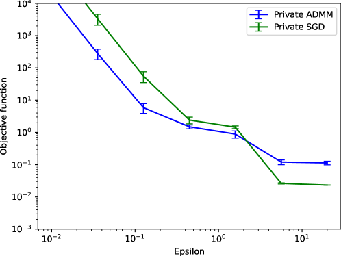
Figure 1: Comparison of DP-SGD and our DP-ADMM algorithm for the Lasso problem on synthetic data ($n=1000$, $p=64$). The same regularizer parameter is used. We show here results for the federated setting, with a user sampling probability of $10\%$. Each setting is run $10$ times, and we report average and standard deviation

The code is available at https://github.com/totilas/padadmm.

References

- Abadi et al. (2016) Abadi, M., Chu, A., Goodfellow, I., McMahan, H. B., Mironov, I., Talwar, K., and Zhang, L. Deep Learning with Differential Privacy. In CCS, 2016.
- Altschuler & Talwar (2022) Altschuler, J. and Talwar, K. Privacy of noisy stochastic gradient descent: More iterations without more privacy loss. In NeurIPS, 2022.
- Balle et al. (2018) Balle, B., Barthe, G., and Gaboardi, M. Privacy Amplification by Subsampling: Tight Analyses via Couplings and Divergences. In NeurIPS, 2018.
- Bassily et al. (2014) Bassily, R., Smith, A., and Thakurta, A. Private Empirical Risk Minimization: Efficient Algorithms and Tight Error Bounds. In FOCS, 2014.
- Bauschke & Combettes (2011) Bauschke, H. H. and Combettes, P. L. Convex Analysis and Monotone Operator Theory in Hilbert Spaces. Springer, 2011.
- Bianchi et al. (2016) Bianchi, P., Hachem, W., and Iutzeler, F. A coordinate descent primal-dual algorithm and application to distributed asynchronous optimization. IEEE Transactions on Automatic Control, 61(10):2947–2957, 2016.
- Bonawitz et al. (2017) Bonawitz, K., Ivanov, V., Kreuter, B., Marcedone, A., McMahan, H. B., Patel, S., Ramage, D., Segal, A., and Seth, K. Practical Secure Aggregation for Privacy-Preserving Machine Learning. In CCS, 2017.
- Boyd et al. (2011) Boyd, S., Parikh, N., Chu, E., Peleato, B., and Eckstein, J. Distributed optimization and statistical learning via the alternating direction method of multipliers. Foundations and Trends® in Machine Learning, 3(1):1–122, 2011.
- Byrne (2003) Byrne, C. A unified treatment of some iterative algorithms in signal processing and image reconstruction. Inverse Problems, 20(1):103–120, 2003.
- Cao et al. (2021) Cao, X., Zhang, J., Poor, H. V., and Tian, Z. Differentially private admm for regularized consensus optimization. IEEE Transactions on Automatic Control (TAC), 66(8):3718–3725, 2021.
- Chaudhuri et al. (2011) Chaudhuri, K., Monteleoni, C., and Sarwate, A. D. Differentially Private Empirical Risk Minimization. Journal of Machine Learning Research, 12(29):1069–1109, 2011.
- Combettes & Pesquet (2019) Combettes, P. L. and Pesquet, J.-C. Stochastic quasi-fejér block-coordinate fixed point iterations with random sweeping ii: mean-square and linear convergence. Mathematical Programming, 174(1):433–451, 2019.
- Combettes & Pesquet (2021) Combettes, P. L. and Pesquet, J.-C. Fixed point strategies in data science. IEEE Transactions on Signal Processing, 69:3878–3905, 2021. ISSN 1941-0476. doi: 10.1109/tsp.2021.3069677. URL http://dx.doi.org/10.1109/TSP.2021.3069677.
- Cyffers & Bellet (2022) Cyffers, E. and Bellet, A. Privacy Amplification by Decentralization. In AISTATS, 2022.
- Cyffers et al. (2022) Cyffers, E., Even, M., Bellet, A., and Massoulié, L. Muffliato: Peer-to-Peer Privacy Amplification for Decentralized Optimization and Averaging. In NeurIPS, 2022.
- Ding et al. (2020) Ding, J., Wang, J., Liang, G., Bi, J., and Pan, M. Towards plausible differentially private admm based distributed machine learning. Proceedings of the 29th ACM International Conference on Information & Knowledge Management, 2020.
- Duchi et al. (2013) Duchi, J. C., Jordan, M. I., and Wainwright, M. J. Local privacy and statistical minimax rates. In FOCS, 2013.
- Dwork & Roth (2014) Dwork, C. and Roth, A. The Algorithmic Foundations of Differential Privacy. Foundations and Trends® in Theoretical Computer Science, 9(3-4):211–407, 2014.
- Eckstein & Yao (2015) Eckstein, J. and Yao, W. Understanding the convergence of the alternating direction method of multipliers: Theoretical and computational perspectives, 2015.
- Feldman et al. (2018) Feldman, V., Mironov, I., Talwar, K., and Thakurta, A. Privacy amplification by iteration. 2018 IEEE 59th Annual Symposium on Foundations of Computer Science (FOCS), Oct 2018. doi: 10.1109/focs.2018.00056. URL http://dx.doi.org/10.1109/FOCS.2018.00056.
- Geyer et al. (2017) Geyer, R. C., Klein, T., and Nabi, M. Differentially private federated learning: A client level perspective. arXiv preprint arXiv:1712.07557, 2017.
- Giselsson & Boyd (2014) Giselsson, P. and Boyd, S. P. Diagonal scaling in douglas-rachford splitting and admm. In CDC, 2014.
- Giselsson et al. (2016) Giselsson, P., Fält, M., and Boyd, S. P. Line search for averaged operator iteration. 2016 IEEE 55th Conference on Decision and Control (CDC), pp. 1015–1022, 2016.
- Hu et al. (2019) Hu, Y., Liu, P., Kong, L., and Niu, D. Learning privately over distributed features: An admm sharing approach. arXiv preprint arXiv:1907.07735, 2019.
- Huang et al. (2019) Huang, Z., Hu, R., Guo, Y., Chan-Tin, E., and Gong, Y. Dp-admm: Admm-based distributed learning with differential privacy. IEEE Transactions on Information Forensics and Security, 15:1002–1012, 2019.
- Iutzeler et al. (2013) Iutzeler, F., Bianchi, P., Ciblat, P., and Hachem, W. Asynchronous distributed optimization using a randomized alternating direction method of multipliers. In CDC, 2013.
- Johansson et al. (2010) Johansson, B., Rabi, M., and Johansson, M. A randomized incremental subgradient method for distributed optimization in networked systems. SIAM Journal on Optimization, 20(3):1157–1170, 2010. doi: 10.1137/08073038X. URL https://doi.org/10.1137/08073038X.
- Kairouz et al. (2021a) Kairouz, P., Diaz, M. R., Rush, K., and Thakurta, A. (Nearly) Dimension Independent Private ERM with AdaGrad Rates via Publicly Estimated Subspaces. In COLT, 2021a.
- Kairouz et al. (2021b) Kairouz, P., Mcmahan, B., Song, S., Thakkar, O., Thakurta, A., and Xu, Z. Practical and private (deep) learning without sampling or shuffling. In ICML, 2021b.
- Kairouz et al. (2021c) Kairouz, P., McMahan, H. B., Avent, B., Bellet, A., Bennis, M., Bhagoji, A. N., Bonawitz, K., Charles, Z., Cormode, G., Cummings, R., D’Oliveira, R. G. L., Eichner, H., Rouayheb, S. E., Evans, D., Gardner, J., Garrett, Z., Gascón, A., Ghazi, B., Gibbons, P. B., Gruteser, M., Harchaoui, Z., He, C., He, L., Huo, Z., Hutchinson, B., Hsu, J., Jaggi, M., Javidi, T., Joshi, G., Khodak, M., Konecný, J., Korolova, A., Koushanfar, F., Koyejo, S., Lepoint, T., Liu, Y., Mittal, P., Mohri, M., Nock, R., Özgür, A., Pagh, R., Qi, H., Ramage, D., Raskar, R., Raykova, M., Song, D., Song, W., Stich, S. U., Sun, Z., Suresh, A. T., Tramèr, F., Vepakomma, P., Wang, J., Xiong, L., Xu, Z., Yang, Q., Yu, F. X., Yu, H., and Zhao, S. Advances and open problems in federated learning. Foundations and Trends® in Machine Learning, 14(1–2):1–210, 2021c.
- Kasiviswanathan et al. (2008) Kasiviswanathan, S. P., Lee, H. K., Nissim, K., Raskhodnikova, S., and Smith, A. D. What Can We Learn Privately? In FOCS, 2008.
- Koloskova et al. (2021) Koloskova, A., Loizou, N., Boreiri, S., Jaggi, M., and Stich, S. U. A unified theory of decentralized sgd with changing topology and local updates, 2021.
- Lian et al. (2017) Lian, X., Zhang, C., Zhang, H., Hsieh, C.-J., Zhang, W., and Liu, J. Can decentralized algorithms outperform centralized algorithms? a case study for decentralized parallel stochastic gradient descent. In NIPS, 2017.
- Liang et al. (2015) Liang, J., Fadili, J., and Peyré, G. Convergence rates with inexact non-expansive operators. Mathematical Programming, 159(1-2):403–434, 2015.
- Lions & Mercier (1979) Lions, P. L. and Mercier, B. Splitting algorithms for the sum of two nonlinear operators. SIAM Journal on Numerical Analysis, 16(6):964–979, 1979.
- Liu et al. (2022) Liu, Y., Geng, J., Shang, F., An, W., Liu, H., Zhu, Q., and Feng, W. Laplacian smoothing stochastic admms with differential privacy guarantees. Trans. Info. For. Sec., 17:1814–1826, jan 2022. ISSN 1556-6013. doi: 10.1109/TIFS.2022.3170271. URL https://doi.org/10.1109/TIFS.2022.3170271.
- Mangold et al. (2022) Mangold, P., Bellet, A., Salmon, J., and Tommasi, M. Differentially Private Coordinate Descent for Composite Empirical Risk Minimization. In ICML, 2022.
- Mao et al. (2020) Mao, X., Yuan, K., Hu, Y., Gu, Y., Sayed, A. H., and Yin, W. Walkman: A communication-efficient random-walk algorithm for decentralized optimization. IEEE Transactions on Signal Processing, 68:2513–2528, 2020. ISSN 1941-0476. doi: 10.1109/tsp.2020.2983167. URL http://dx.doi.org/10.1109/TSP.2020.2983167.
- McMahan et al. (2018) McMahan, H. B., Ramage, D., Talwar, K., and Zhang, L. Learning differentially private recurrent language models. In International Conference on Learning Representations, 2018.
- Mironov (2017a) Mironov, I. Renyi differential privacy. CoRR, abs/1702.07476, 2017a. URL http://arxiv.org/abs/1702.07476.
- Mironov (2017b) Mironov, I. Rényi differential privacy. 2017 IEEE 30th Computer Security Foundations Symposium (CSF), Aug 2017b. doi: 10.1109/csf.2017.11. URL http://dx.doi.org/10.1109/CSF.2017.11.
- Mironov et al. (2019) Mironov, I., Talwar, K., and Zhang, L. Rényi differential privacy of the sampled gaussian mechanism. arXiv preprint arXiv:1908.10530, 2019.
- Noble et al. (2022) Noble, M., Bellet, A., and Dieuleveut, A. Differentially Private Federated Learning on Heterogeneous Data. In AISTATS, 2022.
- Ryu & Boyd (2015) Ryu, E. K. and Boyd, S. P. A primer on monotone operator methods. 2015.
- Ryu et al. (2020) Ryu, E. K., Taylor, A. B., Bergeling, C., and Giselsson, P. Operator splitting performance estimation: Tight contraction factors and optimal parameter selection. SIAM Journal on Optimization, 30(3):2251–2271, 2020.
- Ryu & Kim (2022) Ryu, M. and Kim, K. Differentially Private Federated Learning via Inexact ADMM with Multiple Local Updates. arXiv e-prints, art. arXiv:2202.09409, 2022.
- Shang et al. (2021) Shang, F., Xu, T., Liu, Y., Liu, H., Shen, L., and Gong, M. Differentially private admm algorithms for machine learning. IEEE Transactions on Information Forensics and Security, 16:4733–4745, 2021.
- Shi et al. (2014) Shi, W., Ling, Q., Yuan, K., Wu, G., and Yin, W. On the linear convergence of the admm in decentralized consensus optimization. IEEE Transactions on Signal Processing, 62(7):1750–1761, 2014.
- Talwar et al. (2015) Talwar, K., Guha Thakurta, A., and Zhang, L. Nearly Optimal Private LASSO. NeurIPS, 28, 2015.
- Tavara et al. (2022) Tavara, S., Schliep, A., and Basu, D. Federated learning of oligonucleotide drug molecule thermodynamics with differentially private admm-based svm. In Machine Learning and Principles and Practice of Knowledge Discovery in Databases: International Workshops of ECML PKDD 2021, Virtual Event, September 13-17, 2021, Proceedings, Part II, pp. 459–467. Springer, 2022.
- Vanhaesebrouck et al. (2017) Vanhaesebrouck, P., Bellet, A., and Tommasi, M. Decentralized Collaborative Learning of Personalized Models over Networks. In AISTATS, 2017.
- Wang et al. (2017) Wang, D., Ye, M., and Xu, J. Differentially private empirical risk minimization revisited: Faster and more general. In NeurIPS, 2017.
- Wei & Ozdaglar (2012) Wei, E. and Ozdaglar, A. E. Distributed Alternating Direction Method of Multipliers. In Proceedings of the 51th IEEE Conference on Decision and Control (CDC), pp. 5445–5450, 2012.
- Wei & Ozdaglar (2013) Wei, E. and Ozdaglar, A. E. On the O(1/k) Convergence of Asynchronous Distributed Alternating Direction Method of Multipliers. In IEEE Global Conference on Signal and Information Processing (GlobalSIP), 2013.
- Zhang & Zhu (2017) Zhang, T. and Zhu, Q. Dynamic differential privacy for admm-based distributed classification learning. IEEE Transactions on Information Forensics and Security (TIFS), 12(1):172–187, 2017.
- Zhang et al. (2018) Zhang, X., Khalili, M. M., and Liu, M. Improving the privacy and accuracy of admm-based distributed algorithms. In ICML, 2018.
- Zhou & Li (2022) Zhou, S. and Li, G. Y. Federated learning via inexact admm. Technical report, arXiv:2204.10607, 2022.
- Zhou et al. (2021) Zhou, Y., Wu, S., and Banerjee, A. Bypassing the ambient dimension: Private SGD with gradient subspace identification. In ICLR, 2021.