[1]\fnmYu \surLiu

1]Dalian University of Technology, China

2]National University of Defense Technology, China

Deep Learning for Video-Text Retrieval: a Review

\fnmCunjuan \surZhu Zhucunjuan@163.com \fnmQi \surJia jiaqi@dlut.edu.cn \fnmWei \surChen weichen@nudt.edu.cn \fnmYanming \surGuo guoyanming@nudt.edu.cn liuyu8824@dlut.edu.cn [ [

Abstract

Video-Text Retrieval (VTR) aims to search for the most relevant video related to the semantics in a given sentence, and vice versa. In general, this retrieval task is composed of four successive steps: video and textual feature representation extraction, feature embedding and matching, and objective functions. In the last, a list of samples retrieved from the dataset is ranked based on their matching similarities to the query. In recent years, significant and flourishing progress has been achieved by deep learning techniques, however, VTR is still a challenging task due to the problems like how to learn an efficient spatial-temporal video feature and how to narrow the cross-modal gap. In this survey, we review and summarize over 100 research papers related to VTR, demonstrate state-of-the-art performance on several commonly benchmarked datasets, and discuss potential challenges and directions, with the expectation to provide some insights for researchers in the field of video-text retrieval.

keywords:

deep learning, video-text retrieval, cross-modal representation, feature matching, metric learning

1 Introduction

With the advent of the big data era, video media software (e.g., YouTuBe, TikTok, and Instagram) has become the main way for human beings to learn and entertain. Facing the explosive growth of multimedia information, people urgently need to find efficient ways to quickly search for an item that meets the user’s needs. In particular, the number of videos with different lengths has soared rapidly in recent years, whereas it becomes more time-consuming and difficult to find the target video. Motivated by this, one of the most appropriate solutions is to search for the corresponding video by a language sentence, i.e., Video-Text Retrieval (VTR).

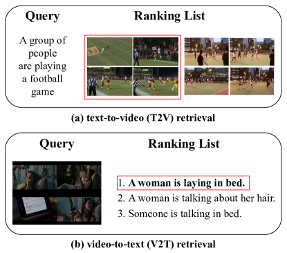
Refer to caption — Figure 1: Video-text retrieval examples on the MSR-VTT dataset. The red box indicates the item is retrieved correctly.

To be more specific, VTR mithun2018learning, guo2021ssan, wang2021t2vlad, gao2021clip2tv, luo2021CLIP4clip, fang2021clip2video, ma2022x, zhao2022centerclip refers to analyze a given sentence so as to find the most matching video from the corpus, and vice versa, as shown in Fig. 1. VTR requires content analysis of a large number of video-text pairs, fully excavating multi-modal information involved, and judging whether the two modalities can be aligned. The majority of vision tasks are longstanding and have achieved excellent results in recent decades, including visual classification, object detection, and semantic segmentation. However, VTR is still an emerging task and has not been studied extensively.

Although the performance of VTR is improving incrementally, there are still some problems and challenges that need further exploration. This review aims to revisit deep learning methods for video-text retrieval and provide an extensive summary for researchers who are devoted to this field. In the following of this section, we will describe the generic pipeline for VTR and the major recent advances.

1.1 Generic Pipeline for VTR

In general, the VTR task can be divided into four parts: video representation extraction, textual representation extraction, feature embedding and matching, and objective functions. Figure 2 depicts the overview pipeline for video-text retrieval.

(1)

Video representation extraction is to capture video feature representation. In this survey, we divide these video feature extractors into spatial feature extractors hu2018squeeze, guo2021ssan, wu2021hanet and temporal feature extractors qiu2019learning, fang2021clip2video, cheng2021improving, han2021visual according to the spatio-temporal property. In addition, since multi-modality information is involved in the videos (e.g., motion, audio, or face features), additional experts are typically used to extract features for each modality, and then are aggregated to generate a more comprehensive video representation miech2018learning, liu2019use, gabeur2020multi, wang2022hybrid.
(2)

Textual representation extraction refers to extract textual features, and the extractors are mainly built upon RNNs otani2016learning, wu2021hanet, CNNs miech2018learning, fan2020person, and Transformer ging2020coot, liu2021hit, gabeur2020multi. Most previous methods dong2019dual, chen2020fine learn and train dual encoders to extract video and textual features separately, but recent work radford2021learning proposes a novel Contrastive Language Image Pre-training (CLIP) model which can learn a multi-modal feature representation in a joint learning fashion. CLIP is composed of an Image Encoder for representing videos and a Language Encoder for textual representations luo2021CLIP4clip, gao2021clip2tv, fang2021clip2video.
(3)

Feature embedding and matching aims to map and align extracted video and text representations and compute their similarity scores (also known as compatibility). The core is how to embed the two modalities in a joint feature space and judge whether they match or not. In order to bridge their semantic gap and measure the similarity more accurately, typical approaches can be divided into global, local, and individual matching according to semantic hierarchy. In addition, most works wang2021t2vlad, dong2022reading, wang2022hybrid consider the combination of global and local features. Furthermore, Min et al. min2022hunyuan_tvr and Wang et al. wang2022disentangled are dedicated to aligning more fine-grained features, i.e., individual-wise. In addition, other recent studies chen2020fine, wu2021hanet, cheng2021improving divide video and text features into the entity, action, and other levels according to the hierarchical semantic graph.
(4)

Objectives functions are to train and refine feature representations from the extractors and similarity scores from feature matching. Existing methods define a variety of objective functions, which can be roughly classified as Triplet loss, Contrastive loss, and other loss. Specifically, triplet losses mainly include bi-directional max-margin ranking loss gabeur2020multi, wang2021t2vlad and hinge-based triplet ranking loss han2021visual. InfoNCE liu2021hit, gao2021clip2tv, ma2022x and Dual Softmax Loss cheng2021improving are commonly utilized for contrastive learning objectives. Additionally, other works introduce knowledge distillation loss croitoru2021teachtext. Moreover, a few studies wu2021hanet, fang2021clip2video choose to combine several loss functions jointly to obtain more optimized results.

1.2 Major Recent Advances

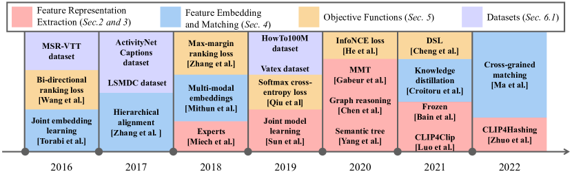
Over the past few years, numerous deep learning methods for both text-to-video and video-to-text have been studied continuously. We depict the representative progresses from 2016 to 2022 in Fig. 3 from four aspects: feature representation extraction, feature embedding and matching, objectives functions, and datasets.

(1)

Feature Representation Extraction. In terms of video and text representation extraction, most existing methods utilize CNNs and RNNs to extract features. Since 2018, some studies begin to extract multi-modal representations with different extractors (also known as experts), and then fuse them to obtain the final video features. Besides, different from building a dual encoder to extract video and text features separately, some works propose learning a joint model to capture multi-modal representation since 2019 sun2019videobert. In 2020, graph reasoning is introduced to the VTR field for learning textual hierarchical features chen2020fine. Likewise, Yang et al. yang2020tree apply a latent semantic tree to capture the relations among the words. Since the proposal of BERT devlin2018bert in 2018, Transformer based approaches have achieved a breakthrough for boosting retrieval performance. Gabeur et al. gabeur2020multi adopt BERT to extract textual features and propose to fuse multi-modal embedding from multiple experts. Since ViT (Vision Transformer) was proposed in 2020, Transformer has become a powerful backbone for recent works like Frozen bain2021frozen and CLIP4Clip luo2021CLIP4clip. Very recently, CLIP4Hashing zhuo2022clip4hashing introduces a hashing encoder that raises a novel idea for feature extraction.
(2)

Feature Embedding and Matching. One of the first works for text-to-video retrieval was in 2016 torabi2016learning, which proposed video-language joint embedding learning to map video and text features into a joint space to bridge the cross-modal gap for better feature matching. Linear projection is a commonly used way for feature embedding, and other nonlinear methods such as clustering centers and MLPs are applicable to perform feature matching. Since 2017, Zhang et al. zhang2018cross have begun to consider the impact of different hierarchical semantic information on feature matching, which gradually evolved into global, local and individual levels as the following years progressed. Besides, Mithun et al. mithun2018learning arise multi-modal embeddings for aligning different modality features. Since the emergence of the cross-encoder model, video and text representations can be concatenated together and fed into a cross-encoder, generating the similarity score via a linear layer. Furthermore, cross-grained similarity calculation ma2022x is first proposed in 2022.
(3)

Objectives functions. For optimizing feature representations, multiple objective functions are defined for the VTR task, for example, bi-directional ranking loss miech2018learning, max-margin ranking loss zhang2018cross, softmax cross-entropy loss qiu2019learning and InfoNCE loss he2020momentum. Notably, Dual Softmax Loss (DSL) cheng2021improving is proposed in 2021, which achieves promising performance gains in many works gao2021clip2tv, luo2021CLIP4clip, min2022hunyuan_tvr.
(4)

Datasets. Since 2016, several large-scale benchmarks such as MSR-VTT xu2016msr, ActivityNet Captions krishna2017dense, LSMDC rohrbach2017movie and HowTo100M miech2019howto100m are collected successively to provide the data support for researching the VTR task. Besides, Vatex wang2019vatex proposed a bilingual dataset in 2019.

Figure 4: Structure of the content in this survey.

Multi-modal video feature (Experts)	Spatial feature extraction		Temporal feature extraction				Textual feature extraction				Method-Year-Results
Multi-modal video feature (Experts)	CNNs	Transf(ViT)	Agg stra.	RNNs	CNNs	Transf	RNNs	CNNs/others	Transf	BERT	Method-Year-Results
✓			✓					✓			MEE miech2018learning2018-10.1(L)
✓			✓					✓			CE liu2019use2019-20.9
✓			✓			✓				✓	MMT gabeur2020multi2020-24.6
✓						✓				✓	HCQ wang2022hybrid2022-25.9
✓			✓							✓	T2VLAD wang2021t2vlad2021-29.5
✓	✓				✓		✓				Fusion mithun2018learning2018-12.5
✓	✓			✓	✓		✓	✓			JsFusion yu2018joint2018-10.2
✓	✓				✓	✓			✓		SUPPORT-SET patrick2020support2020-27.4
✓	✓				✓	✓				✓	HiT liu2021hit2021-28.8
✓	✓	✓			✓	✓				✓	VSR-Net han2021visual2021-37.2
✓		✓			✓	✓				✓	MDMMT dzabraev2021mdmmt2021-38.9
	✓		✓	✓			✓	✓		✓	Dual Enc. dong2019dual2019-7.7(Mfull)
	✓				✓			✓			HowTo100M miech2019howto100m2019-14.9
	✓			✓			✓				TCE yang2020tree2020-17.1
	✓		✓					✓			ClipBERT lei2021less2021-22.0
	✓			✓			✓	✓			Ali et al. ali2022video2022-26.0
	✓			✓		✓				✓	RIVRL dong2022reading2022-27.9
		✓				✓				✓	Frozen bain2021frozen2021-31.0
		✓	✓							✓	MILES ge2022miles2022-37.7
		✓	✓							✓	CAMoE cheng2021improving2021-47.3
		✓			✓	✓			✓		MDMMT-2 kunitsyn2022mdmmt2022-48.5
		✓				✓			✓		CLIP2Video fang2021clip2video2021-45.6
		✓				✓			✓		CLIP2TV gao2021clip2tv2021-52.9
		✓							✓		CenterCLIP zhao2022centerclip2022-48.4
		✓	✓	✓		✓			✓		CLIP4Clip luo2021CLIP4clip2021-44.5
		✓	✓			✓			✓		HunYuantvr min2022hunyuan_tvr2022-55.0
		✓							✓		DRL wang2022disentangled2022-53.3
		✓				✓			✓		X-CLIP ma2022x2022-49.3
		✓	✓						✓		X-Pool gorti2022x2022-46.9
\botrule

Table 1: Overview of feature extractors for videos and sentences based on deep learning. Each ‘✓’ refers to the network that the corresponding work utilizes. The first column indicates the application of experts, which refers to multi-modal video features. The following two columns extract video features from spatial and temporal characteristics. The fourth column presents the use of textual encoders. The last column lists the published papers and reports their performance results on the MSR-VTT 1k-A split.

The rest of this survey paper is organized as shown in Fig. 4. In Section 2, we introduce how to extract video features. Section 3 gives an introduction to existing methods for textual feature extraction. In Section 4, we present how to embed video and text representation into a common space for feature matching. Section 5 describes several objective loss functions widely utilized to train feature representation and matching. In Section 6, we summarize existing large-scale VTR datasets and compare the results of recent methods on these datasets. Afterward, Section LABEL:Challenges_and_Directions introduces the key challenges that are still remaining and discusses several potential directions in near future. Finally, in Section LABEL:conclusion we draw our conclusions.

2 Video Representation Extraction

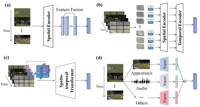
Video representation extraction specifies a way of representing a video. Compared to static image data, video data is a type of information-intensive and complex media, which contains both spatial and temporal representation. Current studies dong2019dual, bain2021frozen, luo2021CLIP4clip are dedicated to learning both spatial and temporal representations. Besides, since the multiple modalities contained in videos, several works devote to multi-modal feature extraction. With the rapid progress of computing resources and the availability of large-scale data, deep learning has become a popular way to capture features. We will detail deep learning approaches for video representation extraction in terms of spatial feature (Section 2.1), temporal feature (Section 2.2) and multi-modal feature (Section 2.3), respectively. The general framework for video representation extraction is illustrated in Fig. 5. In addition, we categorize the video feature extraction methods in Table 1, where the first column lists the approaches that employ multiple expert models, and the second and third columns show the basic networks to extract temporal and spatial representation separately.

2.1 Spatial Feature Extraction

In general, the first step for representing a given video is to select the key frames. The most common approaches for sampling video frames include random sampling (i.e., sampling several frames per second) miech2018learning, sun2019videobert, ging2020coot, ge2022miles, uniformly sampling a fixed number of frames yang2020tree, cheng2021improving, and sparse sampling lei2021less. Afterward, the next step is to extract features for the selected frames. Since each frame in a video is similar to a still image, its spatial feature can be implemented similarly to the still image. Previous methods miech2018learning, mithun2018learning, yu2018joint, dong2019dual are mainly based on CNNs variants, while the Transformer architecture has become widely used since 2018. Overall, we divide existing methods into CNNs-based and Transformer-based spatial feature extractors.

CNNs based methods. Many popular CNNs architectures, including AlexNet krizhevsky2012imagenet, VGGNet simonyan2014very, GoogLeNet szegedy2015going, ResNet he2016deep and DenseNet huang2017densely, have been applicable in extracting the features from sampled video frames. For instance, Torabi et al. torabi2016learning apply a pre-trained VGG-19 model to extract frame-level features from the penultimate layer. Mithun et al. mithun2018learning resize frames and input them into ResNet-152 to capture frame-wise features from the penultimate layer. Likewise, many works mithun2018learning, yang2020tree, liu2021hit extract video appearance features from the global average pooling in a pre-trained ResNet152 or SENet-154 hu2018squeeze. Wang et al. wang2022cross extract frame features from the FC layer whose input is the last average pooling layer in ResNet-152.

Transformer based methods. Transformer vaswani2017attention has developed rapidly and achieved remarkable progress in recent years, which abandons primary neural networks and solely contains stacked encoder-decoder blocks composed of multi-head self-attention (MSA), Multi-Layer Perceptron (MLP), and layer-norm (LN). For instance, VSR-Net han2021visual employs a multi-layer Spatial Transformer block to perform interactions among objects and then adopts average pooling to generate frame representation. Besides, Dosovitskiy et al. dosovitskiy2020image provide a general Vision Transformer (ViT) for extracting image or video frame features. ViT is proposed as a pure transformer architecture for image classification, which generates excellent performances and becomes a strong backbone already cheng2021improving, han2021visual, ge2022miles. To be specific, the first step is to convert a given sampled frame into flattened and discrete $2D$ patches. Then, it projects those non-overlapping patches into $1D$ tokens via linear projection, meanwhile, recording their position and classification information via position and extra learnable $[class]$ embeddings. After feeding them into a Transformer structure, the frame representation is generated from the last layer of the $[CLS]$ token. For instance, CLIP4Clip luo2021CLIP4clip introduces a 3D linear to learn temporal information across frames. Notably, ViT has multiple variants, e.g., ViT B/16, ViT L/14, ViT H/14, and the selection of different models may affect the final results (See Tab. LABEL:finetune_evaluation). Moreover, as the proposal of large-scale pre-training methods, CLIP radford2021learning provides a pre-trained ViT encoder to directly extract vision features. In one word, Transformer has gradually become the mainstream network architecture for VTR gao2021clip2tv, fang2021clip2video, gorti2022x, ma2022x, due to its excellent performance on a variety of public datasets.

2.2 Temporal Feature Extraction

After extracting spatial features, the next step is to model their temporal interaction information. One simple and general manner is aggregating features of the sampled frames via mean pooling mithun2018learning, dong2018predicting, dong2019dual, liu2021hit or max pooling miech2019howto100m, wray2019fine. In addition, temporal features in videos can be modeled by RNNs and CNNs. Moreover, recent state-of-the-art methods exploit Transformer to generate more sophisticated temporal features sun2019videobert, tan2019lxmert, su2019vl.

RNNs based methods. Motivated by the significant performance of RNNs in the field of NLP bengio1994learning, some studies dong2019dual, ali2022video transfer those typical networks, especially GRU networks, to capture long-range temporal features in videos. Concretely, Dong et al. dong2022reading input frame features into bidirectional GRU (biGRU) chung2014empirical to extract temporal information from both forward and backward and then perform mean pooling to generate the whole representation along the temporal dimension. After training biGRU, Dong et al. dong2019dual input the feature maps into 1D CNNs, which includes several filter sizes to capture multi-scale features. Besides, Yang et al. yang2020tree capture temporal features via transforming spatial features extracted from ResNet152 he2016deep to GRU and then aggregate them via an attention module. Despite the fact that RNNs have been applied in many studies, one notable weakness is its expensive training time, in particular for very long-range videos.

CNNs based methods also achieve excellent results for VTR in these years. In terms of 2D CNNs, the work in lin2019tsm has designed a temporal shift module (TSM) which is inserted into the residual branch in ResNet-50 for shifting some channels between frames in the temporal dimension and fusing temporal information among multiple frames. SSAN guo2021ssan demonstrates that learning spatial correlations firstly can provide extra information for better temporal correlations extraction. Compared with 2D CNNs, 3D CNNs add a temporal dimension during moving across the channels, which is favorable for capturing spatio-temporal features. To this end, many approaches directly extend 2D CNNs into 3D CNNs instead tran2015learning, carreira2017quo, tran2017convnet. For instance, Mithun et al. mithun2018learning extract activity (motion) features via I3D carreira2017quo which inflates 2D CNNs to deep 3D CNNs. Res3D tran2017convnet extends all $3\times 3$ convolutional layers in ResNet he2016deep by $3\times 3\times 3$ , which is applied in SlowFast model feichtenhofer2019slowfast that concatenates spatial and temporal features in two branches from dense frames and fewer channels. Besides, Feichtenhofer et al. feichtenhofer2016convolutional demonstrate that fusing spatial features in the last layer with 3D CNNs and replacing 2D pooling with 3D pooling can learn better representation. Substitution of the first three layers also improves performance, as confirmed in karpathy2014large. Furthermore, Hara et al. hara2018can show the effectiveness of building deeper 3D CNNs for large-scale video datasets.

While 3D CNNs bring the above advantages, the retrieval speed, as a significant evaluation metric, has slowed down significantly. To overcome this deficiency, the pseudo-3D CNNs model is proposed sun2015human, qiu2017learning, tran2018closer, which replaces 3D CNNs with spatial 2D CNNs and temporal 1D CNNs. Likewise, Separable 3D (S3D) xie2018rethinking is to substitute 3D CNNs in I3D carreira2017quo, which is commonly utilized for extracting motion features wang2021t2vlad, gabeur2020multi, liu2019use, sun2019learning, sun2019videobert. Additionally, they add gating mechanisms after each 1D CNNs of S3D to generate S3D-G for further improving accuracy. For considering fine-grained features, Local and Global Diffusion (LGD) qiu2019learning is presented to strengthen interactions between local and global feature representation via combining LGD-2D yao2018yh and LGD-3D (a pseudo-3D CNNs qiu2017learning). In a nutshell, applying 2D CNNs to extract spatial features and then utilizing 3D CNNs to capture temporal motion features is a common way for video feature extraction based on CNNs mithun2018learning, han2021visual.

Transformer based methods. In the previous subsection, we have introduced the application of Transformer in spatial feature extraction. In fact, Transformer also has a great ability to capture long-distance temporal relations. a few works gao2021clip2tv, han2021visual, ma2022x, wang2022disentangled propose to build Transformer based models to capture the interaction information between different frames. For example, CLIP2Video fang2021clip2video proposes to model the differences (i.e., motion features) among consecutive adjacent frames and feed them into a temporal Transformer with position and type information to generate temporal features via average pooling. COOT ging2020coot introduces a temporal Transformer to capture frame and clip feature interactions successively. X-CLIP ma2022x applies a three-layer Transformer to encode frame features and averages them to obtain video features. Han et al.han2021visual utilize a multi-layer Transformer to capture spatial features among adjacent frames, and an attention-aware feature aggregation layer to fuse features into a comprehensive representation. In addition, CLIP radford2021learning also provides four layers of temporal transformer blocks (with frame position embedding and residual connection), which is widely employed in numerous works gao2021clip2tv, wang2022disentangled, min2022hunyuan_tvr.

Recently, because of the excellent performance of ViT in capturing spatial representation, many researches bertasius2021space, zhang2021vidtr, arnab2021vivit, bain2021frozen are dedicated to developing novel Transformer networks for learning both spatial and temporal features. Not like the mentioned methods that capture spatial features first and then transfer them into a temporal Transformer, Frozen bain2021frozen proposes a stack of space-time Transformer blocks, which can learn both temporal and spatial position, feed flattened spatial-temporal patch embeddings into temporal and spatial self-attention layers sequentially. Likewise, TimeSformer bertasius2021space introduces a richer study of five spatio-temporal combinations, indicating that the divided space-time scheme achieves the best performance because of its larger training capacity, especially when performing on longer video clips and higher frame resolution. Recent work in Ge et al. ge2022miles applies 12 divided space-time self-attention blocks to obtain feature representation, utilizing masked visual modeling to mask out the local content of consecutive frames and obtain more fine-grained video information.

2.3 Multi-modal Video Feature Extraction

Since the video contains not only spatio-temporal characteristics but also multi-modal information, such as audio, Optical Character Recognition (OCR), and motion. Some works also study how to extract multi-modal video features. For these modalities, additional ‘Experts’ are integrated, each of which is dedicated to extracting features from a specified modality and can be applied directly miech2018learning, liu2019use, gabeur2020multi, wang2021t2vlad. Existing studies dzabraev2021mdmmt, kunitsyn2022mdmmt combine several modality information with spatial-temporal features and demonstrate the ability to enrich final semantic representation. The feature extraction methods for each expert are introduced below.

•

Scene embeddings are extracted from DenseNet-161 huang2017densely trained for image classification on the Places365 dataset zhou2017places.
•

Face features are extracted in two stages: firstly extract bounding boxes via an SSD liu2016ssd face detector, and then pass into ResNet50 that trained for face classification on the VGGFace2 dataset cao2018vggface2.
•

Motion features are extracted from S3D xie2018rethinking and SlowFast feichtenhofer2019slowfast trained on Kinetics action recognition dataset, or I3D carreira2017quo and a 34-layer R(2+1)D tran2018closer trained on IG-65m.
•

Audio features are extracted based on VGGish hershey2017CNN trained on YouTube-8m dataset for audio classification.
•

OCR features are obtained in two steps: the overlaid text is first detected via the pixel link text detection model deng2018pixellink. Then the detected boxes are passed through a text recognition model trained on the Synth90K dataset.
•

Speech transcripts are extracted using the Google Cloud Speech to Text API, with the language set to English. The detected words are then encoded by pre-training word2vecmikolov2013efficient.

After extracting video features of each modality, the primary question is how to perform temporal aggregation to generate video representations composed of multiple expert features. Yu et al. yu2018joint reduce the dimension of extracted audio features and directly concatenate them with visual features to obtain the final video representation. As suggested by Miech et al. miech2018learning and Liu et al. liu2019use, the gating mechanism enables to act as an effective way to predict and choose attention relationships among experts and further to fuse them via average pooling or the VLAD mechanism. Moreover, Shvetsova et al. shvetsova2021everything raise the Multi-modal Fusion Transformer to fuse multi-modal features and realize modality agnostic via training all combinations among different modalities, by averaging them and projecting them together with normalization.

Takeaway for video representation. In this section, we have summarized typical approaches for capturing video representation. Based on the spatio-temporal characteristics within videos, the temporal and spatial features are extracted respectively. CNNs, Transformer, and even RNNs based architectures can be chosen to generate comprehensive video representation for processing frame-wise features, or dividing them into several hierarchies for fine-grained feature interaction. Additionally, more ‘experts’ can be directly utilized to extract more multimedia information. Due to the relatively high performance achieved by CLIP model so far, researchers strike to build appropriate networks according to different task scenarios to extract the most important modality information and generate a more comprehensive video representation.

3 Textual Representation Extraction

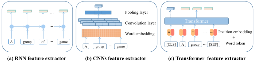
Textual representation extraction aims to extract features from language sentences. The main challenge is how to model sequential relationships to capture complete semantic information. Since the sophisticated developments of NLP with deep neural networks, the capacity for processing long-term dependencies problems is continuously strengthened. At the early stage, word2vec and Glove are adopted to extract word embeddings. Later, RNNs with strong long-distance learning ability have been adopted in more studies otani2016learning, yang2020tree. In some studies, CNNs may achieve semantic representation ability similar to RNNs. Since the recent emergence of Transformer variants, the problem that RNNs cannot operate in parallel has been solved, and a breakthrough in performance has been achieved on many benchmarks. The following sections aim to survey the approaches of textual representation based on RNNs (Section 3.1), CNNs (Section 3.2), and Transformer (Section 3.3). The common strategies for textual representation generation are shown in Fig. 6. Meanwhile, Table 1 summarizes the use of different textual feature extractors.

3.1 RNNs based Textual Feature

Recurrent Neural Networks (RNNs) bengio1994learning are proposed to learn associations between words in the sentences for modeling long sequence data, while the problems of gradient disappearance and gradient explosion arise. To solve the problem, LSTM represents long short-term memory hochreiter1997long, which aims to make up for the problems caused by RNNs via remembering something crucial and choosing unimportant to forget in long sequence data. For instance, to address the problem of long sequence forgetting, Otani et al. otani2016learning utilize RNNs to extract textual features for generating sentence embedding. Bi-directional LSTM (biLSTM) is employed twice in work chen2020fine to obtain contextual-aware word embeddings on graph nodes that are distinguished and generated by off-the-shelf semantic role parsing toolkit song2019polysemous.

GRU chung2014empirical stands for Gated Recurrent Unit, which is a modification based on LSTM. The input gate and the forget gate are combined to generate the update gate, and the cell state and hidden unit are fused as well. Compared with LSTM, the GRU model is simplified with less calculation. The original sentences are input into GRU via the word embedding transformation to obtain text representation mithun2018learning. HANet wu2021hanet utilizes biGRU to select features corresponding to verbs and nouns as individual-level representations. The modified relational GCN schlichtkrull2018modeling is then employed to obtain local and global-level representation. Besides, Tree-structured LSTM tai2015improved is proposed to capture semantic features based on word nodes relationship of tree structure yang2020tree.

3.2 CNNs based Textual Feature

Since 2014, Yoon Kim and other researchers zhang2015sensitivity, chen2015convolutional have introduced CNNs to the NLP domain for extracting better short-range text features with fast calculation, including the related input layer, convolution layer, pooling layer, and fully connected layer. MSSP fan2020person is proposed to recognize the specific person via natural language with bounding boxes, which utilizes 1D CNNs to encode sentences and then captures local features of sentences across multiple scales. Besides, they also choose GRU and Gaussian-Laplacian mixture models to improve the final performance. Miech et al. miech2018learning apply the aggregation module of NetVLAD arandjelovic2016netvlad to aggregate the input word embedding vectors to a global vector representation. Also, caption features are generated from a shallow 1D-CNNs which is built on the top of pre-computed word embeddings miech2019howto100m.

3.3 Transformer based Textual Feature

With the emergence and development of Transformer, it almost replaces RNNs in the NLP field gradually. As BERT is put forward, the development of the NLP field goes to a higher level, and it might be the first choice to extract textual features gabeur2020multi, ging2020coot, liu2021hit, wang2021t2vlad.

BERT is short for Bidirectional Encoder Representations from Transformer devlin2018bert, which includes multiple stacked combinations of Multi-Head Attention, Add & Norm, Feed Forward, and Residual Connection. The sum of token embeddings, segment embeddings, and position embeddings are fed into BERT for learning global semantic information. Token $[CLS]$ situates before the first token of the sentence for text classification, and $[SEP]$ is for separating two sentences. The $[CLS]$ token from the last layer often represents global semantic information. For pre-training, the Masked Language Model (MLM) and Next Sentence Prediction (NSP) are applied to capture more comprehensive word and sentence-level representations, respectively. The core of MLM is masking several words in each sentence randomly and then predicting them by the remaining words. Given two sentences in an article, NSP is applied to determine whether the second sentence follows the first one in the text. BERT has become the most common architecture for the VTR task in recent years. Since the different numbers of encoders and hidden layers, BERT can be divided into BERT-Tiny, BERT Mini, BERT-Small, BERT- Medium, and BERT-Base. BERT-Base is the most commonly applied encoder in many works gabeur2020multi, ging2020coot, liu2021hit, wang2021t2vlad. Besides, due to the differences in case sensitivity, there are BERT-uncased ging2020coot, liu2021hit and BERT-cased wang2021t2vlad.

Moreover, due to the excellent performance achieved by BERT, plenty of BERT-like architectures are proposed successively, e.g., RoBERTa liu2019roberta, ALBERT lan2019albert and DistilBERT sanh2019distilbert. Particularly, DistilBERT sanh2019distilbert introduces knowledge distillation to reduce the model size and inference speed without excessively reducing the performance, which is applied for video-text retrieval tasks such as in Frozen bain2021frozen and MILES ge2022miles. More recently, CLIP radford2021learning provides a Transformer architecture for extracting textual features and achieves state-of-the-art performance in extensive experiments gao2021clip2tv, luo2021CLIP4clip, fang2021clip2video, zhao2022centerclip.

Takeaway for textual representation. First, the application of RNNs solves the problem of long-range feature extraction to a certain extent. While the problems of gradient disappearance and gradient explosion are alleviated in subsequent LSTM and GRU, these models do not process parallel computing due to long-time contextual dependency. Second, CNNs have strong parallel computing capability, but compared with RNNs, they cannot model long-distance features. It can be seen that the number of convolution layers may increase to compensate for this deficiency. Third, compared with RNNs and CNNs, Transformer is currently more widely utilized and its capability of long-term feature extraction is slightly better than RNNs. Besides, Transformer is better in terms of the overall ability to extract text features. The work in radford2021learning compares several typical textual feature extractors.

4 Feature Embedding and Matching

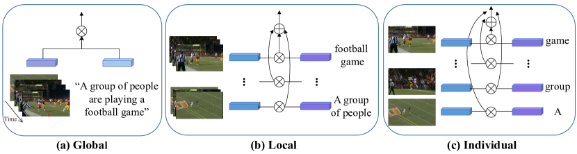
After generating video and textual feature representation, the key is how to project them into a joint embedding space for feature alignment and similarity calculation. Most existing works yang2020tree, luo2020univl only align the global cross-modal features without considering local details. With the gradual mining of hierarchical semantics, some studies chen2020fine, ging2020coot divide features into more fine-grained hierarchical, i.e., local features or even individual features. Finally, combining each level alignment improves the feature matching accuracy. Figure 7 shows the process of video-text matching methods from three categories: Global, Local, and Individual, which are detailed in Section 4.1, Section 4.2 and Section 4.3, respectively. Additionally, Fig. 9 shows the combinations of different granularity matching and lists the representative works for each combination in recent years.

4.1 Global Matching

Global matching aims to project coarse-grained video and text features into a joint embedding space and then perform global similarity computation. Two categories of global matching are depicted in Fig. 8. We take the linear projection and $cosine$ similarity calculation as an example to present the most commonly applied way in Fig. 8(a). Fig. 8 (b) demonstrates the way to capture video and text feature correlations through Transformer and output the predicted score via a linear layer. Next, we detail how to project and calculate these similarities.

Linear projection is the easiest way to map features into low dimension yang2020tree, ging2020coot, bain2021frozen. For instance, ActBERT zhu2020actbert utilizes a linear layer on both “ $[CLS]$ ” tokens of video and text and a $sigmoid$ function to obtain similarity scores. VSR-Net han2021visual adopts a pointwise linear layer and an attention-aware feature aggregation layer to generate video and text embedding vectors for latter matching. Furthermore, linear projection matrices are adopted in works yang2020tree, ali2022video, and X-Pool gorti2022x performs projection with a Layer Normalization layer and a projection matrix. Additionally, non-linear embedding functions are usually implemented by means of FC layers dong2022reading and gating functions miech2018learning, miech2019howto100m. Several studies lu2016event, dong2019dual apply VSE++ faghri2017vse++ for projecting features into a joint embedding space with affine transformation. Besides, MLPs can also be adopted as the nonlinear projection heads to conduct nonlinear transformations liu2021hit. Additionally, Cross encoder is introduced to concatenate video and text features in the temporal dimension with their position embeddings for capturing multi-modal interaction luo2020univl, luo2021CLIP4clip.

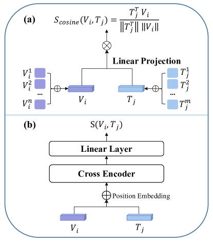
The ways for computing matching scores contain dot-product bain2021frozen, cosine distance, Jaccard function wu2021hanet, and Euclidean distance. Cosine distance is adopted in most works liu2019use, miech2019howto100m, dong2019dual, wu2021hanet. Moreover, a few works ma2022x, ali2022video adopt matrix multiplication between video and text representations to assess similarities. Take CLIP4Clip luo2021CLIP4clip as an example, it divides the similarity calculator into three categories based on whether new parameters are introduced. In this survey, we determine the category of feature matching according to the extracted categories of features used to calculate similarity. Therefore, we consider it as global matching, which generates the global representation by mean pooling and applies cosine similarity to calculate similarity scores for the first two calculators. Additionally, the third “Tight type” realizes cross-modal feature interaction with a Transformer encoder and then generates the prediction score via two linear layers and an activation function.

4.2 Local Matching

Different from global matching, local matching estimates whether the local features (i.e., words and frames) can be aligned or not. Especially, some studies demonstrate that the retrieval performance of global matching is even lower than that of only local matching. However, combing the two strategies can achieve remarkable performance boosts wang2021t2vlad, liu2021hit, han2021visual, ma2022x.

To perform local matching, in addition to projection methods described previously, several feature aggregation and embedding strategies are adopted on word and frame features. Clustering center is a common way, which contains k-means sun2019videobert, NetVLAD arandjelovic2016netvlad and GhostVLAD zhong2018ghostvlad. Generally, local feature embeddings are projected into multiple cluster centers according to soft-aligned weights, which are usually calculated by applying the dot product between features and cluster centers. Those centers are then aggregated and normalized as fine-grained embeddings. At last, similarity calculation is performed on these fine-grained embeddings between video and text to generate local matching scores wang2021t2vlad, wang2022hybrid. For instance, CenterCLIP zhao2022centerclip arises a multi-segment clustering strategy (i.e., k-medoids++ and Spectral clustering) for capturing detailed temporal interaction information and enhancing feature alignment on segment levels. Besides, since experts are utilized to extract multi-modal information in the video, for achieving video-text alignment, most studies liu2019use, gabeur2020multi apply NetVLAD to cluster text features and project them into separate subspaces according to each expert. Considering the different importance of multi-modal features for VTR, a weighted sum of cosine distances can be calculated for different experts miech2018learning, wang2021t2vlad.

In addition to projecting text and video features into a single joint space, other multiple embedding spaces are also exploited to perform alignment and similarity calculations. Mithun et al. mithun2018learning map appearance, audio, and motion features into Object-Text and Activity-Text space separately by multiplying transformation matrices. VSR-Net han2021visual projects text, video features, and relational features into relation and video embedding, and the final similarity is then calculated by multiple embedding spaces respectively. CAMoE cheng2021improving computes similarities from three aspects: entity, sentence, and action.

Like global matching, many approaches apply cosine similarity to estimate local matching mithun2018learning, cheng2021improving, han2021visual. In addition, HiT liu2021hit proposes local features with semantic and feature levels and aligns both positive and negative similarities on these two levels. Besides, a variety of attention mechanisms are used to align each level of features and normalize similarity weights via $softmax$ function chen2020fine, ging2020coot, wu2021hanet. For instance, HANet wu2021hanet utilizes an attention mechanism to enhance local-level cosine similarity and the Jaccard similarity on the concept level. Moreover, matrix multiplication is adopted in work ma2022x to compute cross-grained features similarities. At last, since multiple feature similarity scores of different levels are generated, it is straightforward to sum and average them to represent the final similarity score chen2020fine, wu2021hanet, wang2021t2vlad.

4.3 Individual Matching

Some studies take into account not only global and local feature matching but also a more fine-grained feature hierarchy, i.e., performing feature alignment at the individual level. Generally, several works adopt matrix multiplying to calculate similarities ma2022x, min2022hunyuan_tvr. To be specific, Min et al. min2022hunyuan_tvr extract features with the same dimension and then compute each frame-word pair similarity via dot-product to form a similarity matrix, which is then aggregated to generate the individual similarity score. Wang et al. wang2022disentangled add weights on relational individual pairs via the attention module. HANet wu2021hanet utilizes an attention mechanism to calculate the weighted cosine individual similarity.

Figure 9: Combinations of three matching strategies.

Takeaway for feature embedding and matching. Feature embedding and matching is to map video and textual features into a joint embedding space via linear, nonlinear projection, or clustering centers. According to the fine-grained features, different levels of matching strategies are developed. The final similarity result is obtained by summing and averaging the similarity score from different granularity levels. As can be seen in Fig. 9, more works combine global and local matching, while none of them combine local and individual matching without using global matching yet.

5 Objective Functions

This section introduces objective functions for optimizing and constraining feature representation and matching. Metric learning methods, which include triplet loss and contrastive loss, are mostly utilized to reduce the intra-class distance and increase the inter-class distance. Since VTR is a bidirectional retrieval task, most loss functions are summed in two directions, i.e., $\mathcal{L}_{total}=\left(\mathcal{L}_{t2v}+\mathcal{L}_{v2t}\right)$ . We will detail several typical loss functions below, including triplet loss functions in Sec. 5.1, contrastive loss functions in Sec 5.2, and other loss functions 5.3.

5.1 Triplet Ranking Loss Functions

Ranking loss is to evaluate and modify the similarity scores by measuring the distance between samples. It is firstly proposed to verify face embedding similarities between the anchor-positive and anchor-negative pairs schroff2015facenet. Specific to VTR, the input triplet consists of a positive video-text sample pair and a negative video or text sample. The loss function aims to maximize the distance of unmatched video-text pairs and minimize that of the matched pairs. The commonly adopted triplet ranking loss includes Bi-directional max-margin ranking loss yu2016video, miech2018learning, miech2019howto100m, liu2019use, gabeur2020multi, wang2021t2vlad, kunitsyn2022mdmmt and Hinge-based triplet ranking loss faghri2017vse++, patrick2020support, wu2021hanet, han2021visual. The general formula is denoted by

	$\displaystyle\mathcal{L}=$	$\displaystyle\left[\Delta+S\left(V,T^{-}\right)-S(V,T)\right]_{+}$		(1)
		$\displaystyle+\left[\Delta+S\left(V^{-},T\right)-S(V,T)\right]_{+}$		(1)

where $\Delta$ represents the margin value for the pairwise ranking loss, $S$ denotes the similarity calculated by cosine similarity, $(V,T)$ is the positive pair, $V^{-}$ and $T^{-}$ are the hardest negatives. The operator $[x]_{+}=max(x,0)$ is adopted twice to ensure that the matching samples should be close for both video-to-text and text-to-video retrieval.

For choosing appropriate hard negative examples, most works dong2019dual, mithun2018learning adopt the hardest one that is closest to positive video-text pairs via the $argmax$ function. Besides, TCE yang2020tree demonstrates that choosing the hardest samples may lead to unstable and slow training in large batches, so they choose the top-5 samples to average the cost. In addition, Mithun et al. mithun2018learning introduce a weighting function $L(r_{v/t})=1+1/(N-r+1)$ before each $[.]_{+}$ formula to make positive samples be top-ranking, where $r_{t}$ and $r_{v}$ denote the rank of matching text $t$ or video $v$ in all the compared samples.

5.2 Contrastive Loss Functions

Instead of inputting a triplet, contrastive loss takes positive and negative pairs as input. But its purpose and form are basically consistent with the triplet loss, guiding models to reduce the distance from positives and expand the distance from negatives. For VTR, most studies liu2021hit, sun2019learning, wang2022hybrid, ma2022x are dedicated to multi-modal contrastive learning and introduce several loss functions.

Symmetric cross entropy loss. Cross entropy loss functions are commonly used in the image classification task, while its learning process is very inconsistent for different categories. For some categories, it may quickly overfit to the wrong labels, while the under-fitting state may occur for other categories. Symmetric Cross Entropy fang2021clip2video, luo2021CLIP4clip is proposed to alleviate this problem. However, unlike the classification loss function, the formula in the VTR task is as follows:

\begin{gathered}\mathcal{L}_{v2t}=-\frac{1}{B}\sum_{i}^{B}\log\frac{\exp\left({S}\left(v_{i},t_{i}\right)\right)}{\sum_{j=1}^{B}\exp\left({S}\left(v_{i},t_{j}\right)\right)}\\ \mathcal{L}_{t2v}=-\frac{1}{B}\sum_{i}^{B}\log\frac{\exp\left({S}\left(v_{i},t_{i}\right)\right)}{\sum_{j=1}^{B}\exp\left({S}\left(v_{j},t_{i}\right)\right)}\end{gathered}

(2)

where $B$ is the batch size. Normalized softmax loss (NSL) qiu2019learning, zhai2018classification, bain2021frozen owns the similar formula with an additional temperature hyper-parameter $\tau$ , which is generally obtained by applying the features generated by FC to the Softmax activation function, followed by cross-entropy loss.

Dual softmax loss (DSL) is proposed in CAMoEcheng2021improving to make sure when the similarity sore from T2V is high, the score of V2T should be high as well, which is based on symmetric cross-entropy loss (Equ. 2) and introduces a prior matrix on each $exp$ function. The prior matrices $\operatorname{Pr}^{v2t}$ and $\operatorname{Pr}^{t2v}$ are shown as followed respectively:

		$\displaystyle\operatorname{Pr}_{i,j}^{v2t}=\frac{\exp\left(l\cdot\operatorname{S}\left(v_{i},t_{i}\right)\right)}{\sum_{j=1}^{B}\exp\left(l\cdot\operatorname{S}\left(v_{j},t_{i}\right)\right)}$		(3)
		$\displaystyle\operatorname{Pr}_{i,j}^{t2v}=\frac{\exp\left(l\cdot\operatorname{S}\left(v_{i},t_{i}\right)\right)}{\sum_{j=1}^{B}\exp\left(l\cdot\operatorname{S}\left(v_{i},t_{j}\right)\right)}$		(3)

where $l$ denotes a logit scaling parameter. Since the proposal of the prior matrix, the single-side high score may not appear again so as to reduce computation and achieve higher performance. Especially in work gao2021clip2tv, the retrieval results improve 4.6% performance on MSR-VTT 1k split R@1 metric due to the introduction of DSL.

InfoNCE Loss. In essence, Noise-Contrastive Estimation (NCE) Loss transforms the multiple classification problem solved by Softmax into a binary classification problem, which infers the real distribution via comparing the noisy samples with the noisy samples. Since the presence of multiple positive and negative samples in the VTR task resembles multiple categories, InfoNCE is proposed van2018representation as a self-supervised contrastive loss liu2021hit, gao2021clip2tv, ge2022miles, ma2022x, which is formulated by:

\mathcal{L}=-log\frac{exp\left(S^{vt+}/\tau\right)}{\sum_{i=1}^{1+K_{t}}exp\left(S_{i}^{vt}/\tau\right)}-log\frac{exp\left(S^{tv+}/\tau\right)}{\sum_{i=1}^{1+K_{v}}exp\left(S_{i}^{tv}/\tau\right)}

(4)

where $S^{vt+}$ is the positive similarity generated by cosine similarity. After calculating NCE loss, MILEs ge2022miles utilizes $l_{2}$ regressive objective loss to revise forecast features on the MVM module.

5.3 Other Loss Functions

Distillation Loss. TeachText croitoru2021teachtext defines a novel similarity matrix distillation loss to convey the similarity matrix consistent with that from the student. Hence, the distillation loss is defined as:

\mathcal{L}_{d}=\frac{1}{B}\sum_{i=1}^{B}\sum_{j=1}^{B}\left[l\left(\Phi(i,j),S_{s}(i,j)\right)\right]

(5)

where $\Phi=\Phi\left(S_{1},\ldots,S_{N}\right)=$ $\frac{1}{N}\sum_{k=1}^{N}S_{k}$ is the aggregation of teacher similarity matrices and $S_{s}$ represents student similarity matrix. $l$ denotes the Huber loss, which is defined as:

l (x, y) = {\begin{matrix} \frac{1}{2} (x - y)^{2} & if x-y ≤1, \\ x-y - \frac{1}{2} & otherwise \end{matrix} Cross-Modal Cycle Consistency Loss. C O O T ging2020coot p r e s e n t s a c r o s s - m o d a l c y c l e c o n s i s t e n c y l o s s f o r b e t t e r c r o s s - m o d a l a l i g n m e n t, w h i c h c a n b e a d o p t e d i n b o t h s u p e r v i s e d a n d u n s u p e r v i s e d s c e n a r i o s . T o b e s p e c i f i c, t a k i n g a s e q u e n c e o f v i d e o e m b e d d i n g s {ϑ_i}_i=1^n= {ϑ_1, …, ϑ_n} a n d s e n t e n c e e m b e d d i n g s {δ_i}_=1^m= {δ_1, …, δ_m} a s i n p u t, f i n d i n g s o f t n e a r e s t n e i g h b o r s f r o m b o t h v i d e o - t o - s e n t e n c e a n d s e n t e n c e - t o - v i d e o d i r e c t i o n . T h e l o s s a i m s t o e n f o r c e t h e m o d e l t o l e a r n s e m a n t i c a l l y c y c l e c o n s i s t e n t r e p r e s e n t a t i o n s v i a r e a l i z i n g t h e b i d i r e c t i o n a l s o f t l o c a t i o n i= μ . (7)Equation 7eq.Equationeqs.Equations7¯ϑδi=∑j=1nαjϑj,αj=exp(-∥δi-ϑj∥2)∑k=1nexp(-∥δi-ϑk∥2)¯ϑδi=∑j=1nαjϑj,αj=exp(-∥δi-ϑj∥2)∑k=1nexp(-∥δi-ϑk∥2)μ=∑j=1mβjj,βj=exp(-∥¯ϑ-δj∥2)∑k=1mexp(-∥¯ϑ-δk∥2)μ=∑j=1mβjj,βj=exp(-∥¯ϑ-δj∥2)∑k=1mexp(-∥¯ϑ-δk∥2)LCMC=∥i-μ∥2LCMC=∥i-μ∥2 w h e r e α_j r e p r e s e n t s t h e s i m i l a r i t y s c o r e o f c l i p ϑ_j f r o m s e n t e n c e δ_i . Table 2Table 2tableTabletablesTables2Table 2

Dataset#Videos#Clips#CaptionsDurationAvg.lengthSourceCaption sourceHowTo100M miech2019howto100m1.221M136M136M134,472h6.5minYouTubeManual&AutomaticalMSR-VTT xu2016msr7,18010k200k41.2h20sYouTubeManualActivityNet Captions krishna2017dense20k100k100k849h180sActivityNet caba2015activitynetAutomaticalLSDMC rohrbach2017movie202118,081118,114158h45sMovieManualVatex wang2019vatex41.3k41.3k826k-10sKinetics-600+YouTubeManual2Commonly used datasets for video-text retrievalTable 2Commonly used datasets for video-text retrieval 6section 6sectionSectionsectionsSections6§66DatasetsandResults I n t h i s s e c t i o n, w e i n t r o d u c e s o m e c o m m o n l y - u s e d d a t a s e t s a n d r e p o r t r e t r i e v a l r e s u l t s o n s e v e r a l s t a n d a r d m e t r i c s f o r c o m p a r i s o n a n d a n a l y s i s . 6.1subsection 6.1sectionSectionsectionsSections6.1§6.16.1Datasets S o m e c o m m o n l y - u s e d d a t a s e t s, w h i c h c o n s i s t o f n u m e r o u s v i d e o c l i p s a n d t h e i r c o r r e s p o n d i n g a n n o t a t e d d e s c r i p t i o n s, a r e d e s c r i b e d i n d e t a i l b e l o w . T h e i r c o m p a r i s o n i s i n T a b l e 2 . MSR-VTT xu2016msr i n c l u d e s 10 k c l i p s f r o m 7180 v i d e o s c o m p o s i t e d b y 20 d i f f e r e n t d o m a i n s f r o m t h e Y o u T u b e w e b s i t e, w h i c h i s c o n s t r u c t e d t o a d d r e s s t h e p r o b l e m o f t r a n s l a t i n g v i d e o s t o t e x t s .20 d i f f e r e n t s e n t e n c e s a r e a n n o t a t e d m a n u a l l y b y 1327 w o r k e r s a n d g e n e r a t e 20 k c l i p - s e n t e n c e p a i r s . E a c h c l i p l a s t s b e t w e e n 10 a n d 30 s e c o n d s, a n d t h e w h o l e d a t a s e t t a k e s o v e r 40 h o u r s . I n a d d i t i o n, t h e a u d i o i n f o r m a t i o n i s c o l l e c t e d i n t o t h i s d a t a s e t . G e n e r a l l y, t h e t e s t / t r a i n s p l i t s o w n t h r e e t y p e s : f u l l s p l i t, 1 k - A s p l i t, a n d 1 k - B s p l i t . F o r t h e f u l l s p l i t, t h e r e a r e 7 k v i d e o s f o r t r a i n i n g a n d 3 k v i d e o s f o r t e s t i n g . T h e 1 k - A s p l i t u t i l i z e s 9 k v i d e o s f o r t r a i n i n g a n d 1 k v i d e o s f o r t e s t i n g a n d t h e 1 k - B s p l i t a d o p t s 6.5 k v i d e o s f o r t r a i n i n g a n d 1 k v i d e o s f o r t e s t i n g . T h e t r a i n i n g v i d e o s a r e f r o m t h e o r i g i n a l t r a i n p a r t, a n d t h e r e s t t e s t p a r t a n d 1 k t e s t i n g v i d e o s a r e s e l e c t e d f r o m t h e t e s t p a r t o f t h e f u l l s p l i t . B e s i d e s, t h e r e i s o n l y o n e c a p t i o n a c c o r d i n g t o e a c h v i d e o c l i p f o r 1 k - A a n d 1 k - B s p l i t s . A t p r e s e n t, t h e 1 k - A s p l i t i s t h e m o s t c o m m o n w a y f o r c o m p a r i n g p e r f o r m a n c e, s e e T a b l e 3 . ActivityNet Captions krishna2017dense c o n s i s t o f 20 k v i d e o c l i p s a n d 100 k d e s c r i p t i o n s f r o m A c t i v i t y N e t . E a c h c l i p o n a v e r a g e c o n t a i n s a b o u t 180 s e c o n d s f o r a t o t a l o f 849 h o u r s . E a c h c a p t i o n c o n t a i n s a n a v e r a g e o f 13.48 w o r d s p e r s e n t e n c e w h i c h i s t e m p o r a l l y l o c a l i z e d a n d a n n o t a t e d v i a A m a z o n M e c h a n i c a l T u r k . A t f i r s t, t h i s d a t a s e t i s c o l l e c t e d f o r d e a l i n g w i t h d e t e c t i n g a n d d e s c r i b i n g t h e o v e r l a p e v e n t s t h a t m a y c o n c u r r e n t i n t h e s a m e v i d e o s i m u l t a n e o u s l y . B e s i d e s, t h i s d a t a s e t r e f e r e n c e s d i f f e r e n t c a t e g o r i e s, w h i c h m e a n s o p e n f o r e v e r y d o m a i n . W e f o l l o w t h e c o m m o n e v a l u a t i o n s e t t i n g zhang2018cross, gabeur2020multi t o c o m p a r e t h e r e s u l t s o n t h e “ missing ” v a l 1^{'} s p l i t . LSMDC (L a r g e S c a l e M o v i e D e s c r i p t i o n C h a l l e n g e) rohrbach2017movie c o n t a i n s 118, 081 v i d e o c l i p s a n d 118114 s e n t e n c e s w i t h 158 h o u r s o f v i d e o s e x t r a c t e d f r o m 202 d i s t i n c t m o v i e s, a n d e a c h v i d e o c l i p i s a r o u n d 45 s e c o n d s . T h e d a t a s e t i s a c o m b i n a t i o n o f M - V A D a n d M P I I - M D d a t a s e t s . T h e f o r m e r i n c l u d e s 46, 589 c l i p s a n d 55, 904 s e n t e n c e s, a n d t h e l a t t e r d a t a s e t c o n t a i n s 68, 337 c l i p s a n d 68, 375 s e n t e n c e s . I n a d d i t i o n t o t h e t w o d a t a s e t s a b o v e, o v e r 20 m o v i e v i d e o s a r e c o l l e c t e d c o n s i s t i n g o f 9, 578 c l i p s a s t h e b l i n d t e s t, w h i c h i s o n l y u s e d f o r e v a l u a t i o n . T h e r e m a i n i n g 118 k c l i p - s e n t e n c e p a i r s a r e s p l i t i n t o a t r a i n i n g s e t w i t h 91, 908 v i d e o c l i p s, a v a l i d a t i o n s e t c o n t a i n i n g 6, 542 c l i p s, a n d a p u b l i c t e s t w i t h 10, 053 c l i p s . Vatex wang2019vatex c o n s i s t s o f m o r e t h a n 41, 250 v i d e o s w i t h 825, 000 C h i n e s e a n d E n g l i s h s u b t i t l e s . I n t h e s u b t i t l e s, t h e r e a r e m o r e t h a n 206, 000 p a r a l l e l E n g l i s h - C h i n e s e t r a n s l a t i o n s . T y p i c a l l y, 25, 991 v i d e o c l i p s a r e u s e d f o r t r a i n i n g, 1500 v i d e o c l i p s f o r v a l i d a t i o n, a n d 1500 v i d e o c l i p s f o r t e s t i n g, w h e r e t h e v a l i d a t i o n a n d t e s t s e t s a r e o b t a i n e d b y r a n d o m l y s p l i t t i n g t h e o f f i c i a l v a l i d a t i o n s e t o f 3000 c l i p s i n t o t w o e q u a l p a r t s . HowTo100M miech2019howto100m c o n t a i n s 136 m i l l i o n v i d e o c l i p s s o u r c e d f r o m 1.22 m i l l i o n n a r r a t e d i n s t r u c t i o n a l v i d e o s o n Y o u T u b e w i t h 12 c a t e g o r i e s a n d r e f e r e n c e d t o 23.6 k v i s u a l t a s k s (e . g ., F o o d a n d E n t e r t a i n i n g, H o b b i e s a n d C r a f t s, a n d S p o r t s a n d F i t n e s s) . E a c h v i d e o c l i p l a s t s a r o u n d 6.5 m i n u t e s, a n d t h e d a t a s e t t a k e s u p 134, 472 h o u r s . T h e 136 m i l l i o n a n n o t a t i o n s a r e g e n e r a t e d v i a a u t o m a t i c a l l y t r a n s c r i b e d n a r r a t i o n b y Y o u T u b e A S R o r t r a n s l a t e d b y Y o u T u b e A P I . A t p r e s e n t, t h e H o w T o 100 M d a t a s e t i s c o m m o n l y a p p l i e d a s a p r e - t r a i n e d d a t a s e t a n d t h e n t r a n s f e r r e d t o o t h e r f i n e - t u n i n g d a t a s e t s (e . g ., M S R - V T T o r L S M D C) . Table 3Table 3tableTabletablesTables3Table 3


MethodText→VideoVideo→TextR@1↑R@5↑R@10↑MdR↓MnR↓R@1↑R@5↑R@10↑MdR↓MnR↓OthersFusion mithun2018learning7.020.929.738.0213.812.532.142.416.0134.0JSFusion yu2018joint10.231.243.213.0------HT MIL-NCE miech2019howto100m14.940.252.89.0------ActBERT zhu2020actbert16.342.856.910.0------HERO li2020hero16.843.457.7-------TCE yang2020tree17.139.953.79------Vidtranslate korbar2020video17.441.653.68.0------ViSERN18.148.461.3628.624.346.259.5734.6CE liu2019use20.948.862.46.028.220.650.364.05.325.1UniVL luo2020univl21.249.663.16.0------ClipBERT lei2021less22.046.859.96.0------SSAN guo2021ssan24.449.3--------MMT gabeur2020multi24.654.067.14.026.724.456.067.84.023.6HCQ wang2022hybrid25.954.869.05.0-26.357.070.14.0-Ali et al. ali2022video26.056.7-3.0-26.756.5-3.0-MMT-pretrained gabeur2020multi26.657.169.64.024.027.057.569.73.7-SUPPORT-SET patrick2020support27.456.367.73.0-26.655.167.53.0-RIVRL dong2022reading27.959.371.24.042.0-----HiT liu2021hit28.860.372.3-327.759.272.0-3T2VLADwang2021t2vlad29.55970.14-31.86071.13-TEACHTEXTcroitoru2021teachtext29.661.674.23------FROZEN bain2021frozen31.059.570.53.0------VSR-Nethan2021visual37.273.885.0-240.276.186.2-2BridgeFormerge2022bridgeformer37.664.875.13.0-33.258.068.64.025.7MILES ge2022miles37.763.673.83.0------CLIP-basedCLIP radford2021learning31.253.764.24.0-27.251.762.65.0-MDMMT dzabraev2021mdmmt38.969.079.72.016.5-----CLIP4Clip luo2021CLIP4clip44.571.481.62.015.342.770.980.62.0-CLIP2Videofang2021clip2video45.672.681.72.014.643.572.382.12.010.2X-Pool gorti2022x46.972.882.22.014.3-----CAMoE cheng2021improving47.374.284.52.011.949.174.384.32.09.9CenterCLIP zhao2022centerclip48.473.882.02.013.847.775.083.32.010.2MDMMT-2 kunitsyn2022mdmmt48.575.483.92.013.8-----X-CLIP ma2022x49.375.884.82.012.248.976.884.52.08.1CLIP2TV gao2021clip2tv52.978.586.51.012.854.177.485.71.09.0DRL wang2022disentangled53.380.387.61.0-56.279.987.41.0-HunYuan_tvr min2022hunyuan_tvr55.080.486.81.010.355.578.485.81.07.73Retrieval results on MSR-VTT 1k-A split. The second part introduces the methods based on the large-scale pre-trained model–CLIP, and the methods in the first part are based on other backbones.Table 3Retrieval results on MSR-VTT 1k-A split. The second part introduces the methods based on the large-scale pre-trained model–CLIP, and the methods in the first part are based on other backbones. Table 4Table 4tableTabletablesTables4Table 44Retrieval results on three benchmarked datasets: ActivityNet Caption, LSMDS and Vatex.Table 4Retrieval results on three benchmarked datasets: ActivityNet Caption, LSMDS and Vatex.MethodText→VideoVideo→TextR@1↑R@5↑R@10↑MdR↓MnR↓R@1↑R@5↑R@10↑MdR↓MnR↓Retrieval performance on ActivityNet Caption krishna2017denseMMTgabeur2020multi22.754.293.25.020.822.954.893.14.321.2HiT liu2021hit27.758.694.74.0T2VLAD wang2021t2vlad23.755.593.5424.156.694.14COOT ging2020coot60.886.698.6160.987.498.61CLIP4Clip-meanPooling luo2021CLIP4clip40.572.498.12.07.442.574.185.82.06.6CE liu2019use17.746.6-6.0------SUPPORT patrick2020support28.760.8-2.0------DRL wang2022disentangled46.277.388.22.0-45.776.587.82.0-X-CLIP ma2022x46.275.56.846.475.96.4HunYuan_tvr min2022hunyuan_tvr57.384.893.11.04.057.785.793.91.03.4Retrieval performance on LSMDC rohrbach2017movieNoiseE amrani2021noise6.419.828.439.0------JSFusion yu2018joint9.121.234.136.0------MEE miech2018learning10.125.634.627------CE liu2019use11.226.934.825.3------MMT gabeur2020multi12.929.940.119.375.012.328.638.920.076.0Frozen bain2021frozen15.030.839.820.0------TeachText-CE+ croitoru2021teachtext17.236.546.313.7------MILES ge2022miles17.835.644.115.5------MDMMT dzabraev2021mdmmt18.838.547.912.358.0-----CLIP4Clip-meanP luo2021CLIP4clip20.738.947.213.065.3-----CLIP4Clip-seqTransf luo2021CLIP4clip22.641.049.111.061.020.839.048.61254.2X-Pool gorti2022x25.243.753.58.053.2-----CAMoE cheng2021improving25.946.153.7-54.4-----X-CLIP ma2022x26.148.446.726.946.241.9MDMMT-2 kunitsyn2022mdmmt26.946.755.96.748.0-----DRL wang2022disentangled26.547.656.87.0-27.045.755.48.0-HunYuan_tvr min2022hunyuan_tvr29.746.455.47.056.430.147.555.77.048.9Retrieval performance on Vatex wang2019vatexHANet wu2021hanet36.474.184.1249.179.586.22VSE faghri2017vse++28.064.376.93.0------SE++33.770.181.02.0------Dual Enc. dong2019dual31.167.578.93.0------HGR chen2020fine35.173.583.52.0------CLIP radford2021learning39.772.382.22.012.852.788.894.91.03.8SUPPORT-SET patrick2020support44.982.189.71.0-58.484.491.01.0-CLIP4Clip-seqTransf luo2021CLIP4clip55.989.295.01.03.973.297.199.11.01.7CLIP2Video fang2021clip2video57.390.095.51.03.67697.799.91.01.5DRL wang2022disentangled65.792.696.71.0-80.198.599.51.0-. 6.2subsection 6.2sectionSectionsectionsSections6.2§6.26.2EvaluaitonM

(8)