Graph Neural Networks with Learnable and Optimal Polynomial Bases

Abstract

Polynomial filters, a kind of Graph Neural Networks, typically use a predetermined polynomial basis and learn the coefficients from the training data. It has been observed that the effectiveness of the model is highly dependent on the property of the polynomial basis. Consequently, two natural and fundamental questions arise: Can we learn a suitable polynomial basis from the training data? Can we determine the optimal polynomial basis for a given graph and node features?

In this paper, we propose two spectral GNN models that provide positive answers to the questions posed above. First, inspired by Favard’s Theorem, we propose the FavardGNN model, which learns a polynomial basis from the space of all possible orthonormal bases. Second, we examine the supposedly unsolvable definition of optimal polynomial basis from Wang & Zhang (2022) and propose a simple model, OptBasisGNN, which computes the optimal basis for a given graph structure and graph signal. Extensive experiments are conducted to demonstrate the effectiveness of our proposed models. Our code is available at https://github.com/yuziGuo/FarOptBasis.

Proof.

1 Introduction

2 Background and Preliminaries

2.1 Background of Spectral GNNs

In this section, we provide some necessary backgrounds of spectral graph neural networks, and show how the choice of polynomial bases emerges as a problem. Notations used are summarized in Table 6 in Appendix A.

Graph Fourier Transform.  Consider an undirected and connected graph $G=(V,E)$ with $N$ nodes, its symmetric normalized adjacency matrix and laplacian matrix are denoted as $\hat{P}$ and $\hat{L}$, respectively, $\hat{L}={I}-\hat{P}$. Graph Fourier Transform, as defined in the spatial/spectral domain of graph signal processing, is analogous to the time/frequency domain Fourier Transform (Hammond et al., 2009; Shuman et al., 2013) . One column in the representations of $N$ nodes, $X\in\mathbb{R}^{N\times d}$, is considered a graph signal, denoted as $x$. The complete set of $N$ eigenvectors of $\hat{L}$, denoted as $U$, who show varying structural frequency characteristics (Shuman et al., 2013), are used as frequency components. Graph Fourier Transform is defined as $\hat{x}:=U^{\mathrm{T}}x$, where signal $x$ is projected to the frequency responses of all components. It is then followed by modulation, which suppresses or strengthens certain frequency components, denoted as $\hat{x}^{*}:=\operatorname{diag}\{\theta_{0},\cdots,\theta_{N-1}\}\hat{x}$. After modulation, inverse Fourier Transform: $x^{*}:=U\hat{x}^{*}$ transforms $\hat{x}^{*}$ back to the spatial domain. The three operations form the process of spectral filtering: $U\operatorname{diag}\{\theta_{0},\theta_{1},\ldots,\theta_{N-1}\}U^{\mathrm{T}}x~{}(1)$.

Polynomial Approximated Filtering.  In order to avoid time-consuming eigendecomposition, a line of work approximate $\theta_{i}$ by some polynomial function of $\lambda_{i}$, which is the $i$-th eigenvalue of $\hat{L}$, i.e. $\theta_{i}\approx h(\lambda_{i})$. Equation (2.1) then becomes a form that is easy for fast localized calculation: $U\operatorname{diag}\{h(\lambda_{0}),h(\lambda_{1}),\dots,h(\lambda_{N-1})\}U^{\mathrm{T}}x=h(\hat{L})x.$ As listed in Introduction, various polynomial bases have been utilized, denoted as ${h(\lambda)=\sum^{K}_{k=0}\alpha_{k}g_{k}(\lambda)}$. For further simplicity, we equivalently use $b(\hat{P})$ instead of $h(\hat{L})$ in this paper, where $b(\hat{P}):=h(I-\hat{P})$. Note that $b(\cdot)$ is defined on the spectrum of $\hat{P}$, and the $i$-th eigenvalue of $\hat{P}$, denoted as $\mu_{i}$, equals $1-\lambda_{i}$.

The filtering process on the input signal $x$ is then expressed as $x\rightarrow z=\sum_{k=0}^{K}\alpha_{k}g_{k}(\hat{P})x$. When consider independent filtering on each of the $d$ channels in $X$ simultaneously, the multichannel filtering can be denoted as: $X\rightarrow Z=\underset{l\in[1,h]}{\|}\sum_{k=0}^{K}\alpha_{k,l}g_{k,l}(\hat{P})X_{:,l}~{}(2)$.

2.2 Orthogonal and Orthonormal Polynomials

In this section, we give a formal definition of orthogonal and orthonormal polynomials, which plays a central role in the choosing of polynomial bases (Simon, 2014).

Inner Products. The inner product of polynomials is defined as $\langle f,g\rangle:=\int_{a}^{b}f(x)g(x)w(x)\mathrm{d}x$, where $f$, $g$ and $w$ are functions of $x$ on interval $(a,b)$, and the weight function $w$ should be non-negative to guarantee the positive-definiteness of inner-product space.

The definition of the inner products induces the definitions of norm and orthogonality. The norm of polynomial $f$ is defined as: $\displaystyle\|f\|=\sqrt{\langle f,f\rangle}$, and $f$ and $g$ are orthogonal to each other when $\displaystyle\langle f,g\rangle=0$. Notice that the concept of inner product, norm, and orthogonality are all defined with respect to some weight function.

Orthogonal Polynomials. A sequence of polynomials $\{p_{n}(x)\}_{n=0}^{\infty}$ where $p_{n}(x)$ is of exact degree $n$, is called orthogonal w.r.t. the positive weight function $w(x)$ if, for $m,n=0,1,2,\cdots$, there exists $\langle p_{n},p_{m}\rangle=\delta_{mn}\|p_{n}\|^{2}(\|p_{n}\|^{2}\neq 0)$, where the inner product $\langle f,g\rangle$ is defined w.r.t. $w(x)$. When $\|p_{n}\|^{2}=1$ for $n=0,1,2,\cdots$, $\{p_{n}(x)\}_{n=0}^{\infty}$ is known as orthonormal polynomial series.

When a weight function is given, the orthogonal or orthonormal series with respect to the weight function can be solved by Gram-Schmidt process.

Remark 2.1.

In this paper, the orthogonal/orthonormal polynomial bases we consider are truncated polynomial series, i.e. the polynomials that form a basis are of increasing order.

3 Learnable Basis via Favard’s Theorem

Empirically, spectral GNNs with different polynomial bases vary in performance on different datasets, which leads to two observations: (1) the choice of bases matters; (2) whether a basis is preferred might be related to the input, i.e. different signals on their accompanying underlying graphs.

For the first observation, we notice that up to now, polynomial filters pick polynomial bases from well-studied polynomials, e.g. Chebyshev polynomials, Bernstein polynomials, etc, which narrows down the range of choice. For the second observation, we question the reasonableness of fixing a basis during training. A related effort is made by JacobiConv (Wang et al., 2019), who adapt to a Jacobi polynomial series from the family of Jacobi polynomials via hyperparameter tuning. However, the range they choose from is discrete. Therefore, we aim at dynamically learn polynomial basis from the input from a vast range.

3.1 Recurrence Formula for Orthonormal Bases

Input: Input signals $X$ with $d$ channels; Normalized graph adjacency $\hat{P}$; Truncated polynomial order $K$

parameter : $\beta$, $\gamma$, $\alpha$

Output: Filtered Signals $Z$

1 $x_{-1}\leftarrow 0$

2 for $l=0$ to $d-1$ do

3      $x\leftarrow X_{:,l}$ , $x_{0}\leftarrow x/\sqrt{\beta_{0,l}}$ ,  $z\leftarrow\alpha_{0,l}x_{0}$

4      for $k=0$ to $K$ do

5           $x_{k+1}\leftarrow(\hat{P}x_{k}-\gamma_{k,l}x_{k}-\sqrt{\beta_{k,l}}x_{k-1})/\sqrt{\beta_{k+1,l}}$

6           $z\leftarrow z+\alpha_{k+1,l}x_{k+1}$

7           $Z_{:,l}\leftarrow z$

return Z  

Algorithm 1 FavardFiltering

Input: Raw features $X_{\textrm{raw}}$; Normalized graph adjacency $\hat{P}$; Truncated polynomial order $K$

parameter : $W_{0}$, $b_{0}$, $W_{1}$, $b_{1}$, $\beta$, $\gamma$, $\alpha$

Output: Label predictions $\hat{Y}$

1 $X\leftarrow X_{\operatorname{raw}}W_{0}+b_{0}$

2 $Z\leftarrow$FavardFiltering($X$, $\hat{P}$, $K$, $\beta$, $\gamma$, $\alpha$)

$\hat{Y}\leftarrow$Softmax($ZW_{1}+b_{1}$)  

Algorithm 2 FavardGNN (For Classification)

Luckily, the Three-term recurrences and Favard’s theorem of orthonormal polynomials provide a continuous parameter space to learn basis. Generally speaking, three-term recurrences states that every orthonormal polynomial series satisfies a very characteristic form of recurrence relation, and Favard’s theorem states the converse.

Theorem 3.1 (Three Term Recurrences for Orthonormal Polynomials).

(Gautschi, 2004, p. 12) For orthonormal polynomials $\{p_{k}\}_{k=0}^{\infty}$ w.r.t. weight function $w$, suppose that the leading coefficients of all polynomials are positive, there exists the three-term recurrence relation:

$$\hbox{\pagecolor{gray!10}$\sqrt{\beta_{k+1}}$}p_{k+1}(x) =(x-\gamma_{k})p_{k}(x)-\hbox{\pagecolor{gray!10}$\sqrt{\beta_{k}}$}p_{k-1}(x),$$

$$p_{-1}(x):=0,\ p_{0}(x)=1/\sqrt{\beta_{0}},$$

$$\gamma_{k}\in\mathbb{R},\ \sqrt{\beta_{k}}\in\mathbb{R}^{+},\ k\geq 0$$ (3)

with $\beta_{0}=\int w(x)\mathrm{d}x$.

Theorem 3.2 (Favard’s Theorem; Orthonormal Case).

(Favard, 1935), (Simon, 2005, p. 14) A polynomial series $\{p_{k}\}_{k=0}^{\infty}$ who satisfies the recurrence relation in Equation (B.5) is orthonormal w.r.t. a weight function $w$ that $\beta_{0}=\int w(x)\mathrm{d}x$.

By Theorem 3.2, any possible recurrences with the form (B.5) defines an orthonormal basis. By Theorem 3.1, such a formula covers the whole space of orthonormal polynomials. If we set $\{\sqrt{\beta_{k}}\}$ and $\{\gamma_{k}\}$ to be learnable parameters with $\sqrt{\beta_{k}}>0(k\geq 0)$, any orthonormal basis can be obtained.

We put the more general orthogonal form of Theorem 3.1 and Theorem 3.2 in Appendix B.1 to B.5. In fact, the property of three-term recurrences for orthogonal polynomials has been used multiple times in the context of current spectral GNNs to reuse $g_{k}(\hat{P})x$ and $g_{k-1}(\hat{P})x$ for the calculation of $g_{k+1}(\hat{P})x$. Defferrard et al. (2016) owe the fast filtering of ChebNet to employing the three-term recurrences of Chebyshev polynomials (the first kind, which is orthogonal w.r.t. $\frac{1}{\sqrt{x^{2}-1}}$): $T_{k+1}(x)=2xT_{k}(x)-T_{k-1}(x)$. Similarly, JacobiConv (Wang & Zhang, 2022) employs the three-term recurrences for Jacobi polynomials (orthogonal w.r.t. to $(1-x)^{a}(1+x)^{b}$). In this paper, however, we focus on orthonormal bases because they minimize the mutual influence of basis polynomials and the influence of the unequal norms of different basis polynomials.

3.2 FavardGNN

Formulation of FavardGNN. We formally write the architecture of FavardGNN (Algorithm 2), with the filtering process illustrated in FavardFiltering (Algorithm 1). Note that the iterative process of Algorithm 1 (lines 3-5) follows exactly from Equation (B.5) in Favard’s Theorem. The key insight is to treat the coefficients $\beta,\gamma,\alpha$ in Equation (B.5) as learnable parameters. Since Theorem 3.1 and Theorem 3.2 state that the orthonormal basis must satisfy the employed iteration and vice versa, it follows that the model can learn a suitable orthonormal polynomial basis from among all possible orthonormal bases.

Following convention, before FavardFiltering, an MLP is used to map the raw features onto the signal channels (often much less than the dimension of raw features). In regression problems, the filtered signals are directly used as predictions; for classification problems, they are combined by another MLP followed by a softmax layer.

Parallel Execution. Note that for convenience of presentation, we write the FavardFiltering Algorithm in a form of nested loops. In fact, the computation on different channels (the inner loop $k$) is conducted simultaneously. We put more concrete implementation in PyTorch-styled the pseudocode in Appendix C.1.

3.3 Weaknesses of FavardGNN

However, there are still two main weaknesses of FavardGNN. Firstly, the orthogonality lacks interpretability. The weight function $w$ can only be solved analytically in a number of cases (Geronimo & Van Assche, 1991). Even if the weight function is solved, the form of $w$ might be too complicated to understand.

Secondly, FavardFiltering is not good in convergence properties: consider a simplified optimization problem $\min\|Z-Y\|^{2}_{\textrm{F}}$ which has been examined in the context of GNN (Xu et al., 2021; Wang & Zhang, 2022), even this problem is non-convex w.r.t the learnable parameters in $Z$. We will re-examine this problem in the experiment section.

4 Achieving Optimal Basis

Although FavardGNN potentially reaches the whole space of orthonormal polynomial series, on the other hand, we still want to know: whether there is an optimal and accessible basis in this vast space.

Recently, Wang & Zhang (2022) raises a criterion for optimal basis. Since different bases are the same in expressiveness, this criterion is induced from an angle of optimization. However, Wang & Zhang (2022) believe that this optimal basis is unreachable. In this section, we follow this definition of optimal basis, and show how we can exactly apply this optimal basis to our polynomial filter with $O(K|E|)$ time complexity.

Wang & Zhang (2022) make an essential step towards this question: they derive and define an optimal basis from the angle of optimization. However, they do not exhaust their own finding in their model, since based on a habitual process, they believe that the optimal basis they find is inaccessible. In this section, we show how we can exactly apply this optimal basis to our polynomial filter in $O(K|E|)$ time complexity.

4.1 A Review: A Definition for Optimal Basis

We start this section with a quick review of the related part from Wang & Zhang (2022), with a more complete review put in Appendix E.

Definition of Optimal Basis.  Wang & Zhang (2022) considers the squared loss $R=\frac{1}{2}\|Z-Y\|_{\textrm{F}}^{2}$, where $Y$ is the target signal. Since each signal channel contributes independently to the loss, the authors then consider the loss function channelwisely and ignore the index $l$, that is, $r=\frac{1}{2}\|z-y\|^{2}_{\textrm{F}}$, where $z=\sum_{k=0}^{K}\alpha_{k}g_{k}(\hat{P})x$.

The task at hand is to seek a polynomial series $\{g_{k}\}_{k=0}^{K}$ which is optimal for the convergence of coefficients $\alpha$. Since $r$ is convex w.r.t. $\alpha$, the gradient descent’s convergence rate reaches optimal when the Hessian matrix is identity. The $(k_{1},k_{2})$ element $(k_{1},k_{2}\in\left[0,K\right])$ of the Hessian matrix is:

$$H_{k_{1}k_{2}}=\frac{\partial^{2}r}{\partial\alpha_{k_{1}}\partial\alpha_{k_{2}}}=x^{\mathrm{T}}g_{k_{2}}(\hat{P})g_{k_{1}}(\hat{P})x.$$ (4)

Wang & Zhang (2022) further reveal the orthonormality inherent in the optimal basis by rephrasing Equation (4) into $H_{k_{1}k_{2}}=\int_{\mu=-1}^{1}g_{k_{1}}(\mu)g_{k_{2}}(\mu)f(\mu)\mathrm{d}\mu$, where the form of $f$ is given in Proposition 4.2 and and derivation is delayed in Appendix E. Combining Definition 4.1, we soonly get:

Unachievable Algorithm Towards Optimal Basis.

Now we illustrate why Wang & Zhang (2022) believe that though properly defined, this optimal basis is unachievable, and how they took a step back to get their final model. We summarize the process they thought of in Algorithm 3. This process is quite habitual: with the weight function in Proposition 4.2 solved, it is natural to use it to determine the first $K$ polynomials by the Gram-Schmidt process and then use the solved polynomials in filtering as other bases, e.g. Chebyshev polynomials. This process is unreachable due to the eigendecomposition step, which is essential for the calculation of $f$ (see Proposition 4.2), but prohibitively expensive for larger graphs.

Input: Graph signal $x$; Normalized graph adjacency $\hat{P}$; Truncated polynomial order $K$

Output: Optimal basis ${\{g_{k}(\cdot)}\}_{k=0}^{K}$

1 $U,\{\mu_{i}\}_{i=1}^{N}\leftarrow$ Eigendecomposition of $\hat{P}$

2 Calculate $f(\mu)$ as descripted in Proposition 4.2

3 Use Gram-Schmidt process and weight function $f(\mu)$ to contruct an orthonormal basis $\{g_{k}\}_{k=0}^{K}$

Apply $\{g_{k}\}_{k=0}^{K}$ in polynomial filtering  

Algorithm 3 (An Unreachable Algorithm for Utilizing Optimal Basis)

As a result, Wang & Zhang (2022) came up with a compromise. They allow their model, namely JacoviConv, to choose from the family of orthogonal Jacobi bases, who have ”flexible enough weight functions”, i.e., $(1-\mu)^{a}(1+\mu)^{b}\left(\forall a,b\in\left(0,1\right)\right)$. In their implementation, $a$ and $b$ are discretized and chosen via hyperparameter tuning. Obviously, the fraction of possible weight functions JacoviConv can cover is still small, very possibly missing the optimal weight function in Proposition 4.2.

4.2 OptBasisGNN

In this section, we show how the polynomial filter can employ the optimal basis in Definition 4.1 efficiently via an innovative $O(K|E|)$ methodology. Our method does not follow the convention in Algorithm 3 where four progressive steps are included to solve the optimal polynomial bases out and utilize them. Instead, our solution to the optimal bases is implicit, accompanying the process of solving a related vector series. Thus, our method bypasses the untractable eigendecomposition step.

Optimal Vector Basis with Accompanying Polynomials.  Still, we consider graph signal filtering on one channel, that is, $x\rightarrow z=\sum_{k=0}^{K}\alpha_{k}g_{k}(\hat{P})x$. Instead of taking the matrix polynomial $b(\hat{P})=\sum_{k=0}^{K}\alpha_{k}g_{k}(\hat{P})$ as a whole, we now regard $\{v_{k}|v_{k}:=g_{k}(\hat{P})x\}_{k=0}^{K}$ as a vector basis. Then the filtered signal $z$ is a linear combination of the vector basis, namely $x\rightarrow z=\sum_{k=0}^{K}\alpha_{k}v_{k}~{}(5)$. When $\{g_{k}\}_{k=0}^{K}$ meets Definition 4.1, for all $k_{1},k_{2}\in[0,K]$, the vector basis satisfies:

$$v_{k_{2}}^{\mathrm{T}}v_{k_{1}}=x^{\mathrm{T}}g_{k_{2}}(\hat{P})g_{k_{1}}(\hat{P})x=\delta_{k_{1}k_{2}}.$$ (6)

Given $(\hat{P},x)$, we term $g_{k}$ the accompanying polynomial of a vector $v_{k}$ if $v_{k}=g_{k}(\hat{P})x$. Note that an accompanying polynomial does not always exists for any vector. Following Equation (6), finding the optimal polynomial basis for filtering is equivalent to finding a vector basis $\{v_{k}\}_{k=0}^{K}$ that satisfies two conditions: Condition 1: Orthonormality; Condition 2: Accompanied by the optimal polynomial basis, that is, $v_{k}\equiv g_{k}(\hat{P})x$ establishes for each $k$, where $g_{k}$ follows Definition 4.1. We term such $\{v_{k}\}$ the optimal vector basis.

Input: Input signals $X$ with $d$ channels; Normalized graph adjacency $\hat{P}$; Order $K$

parameter : $\alpha$

Output: Filtered signals $Z$

5 for $l=0$ to $d-1$ do

6      $x\leftarrow X_{:,l}$

      $v_{0}\leftarrow x/\|x\|$ ;

       // $g_{0}(\mu)=1/\|x\|$

7      $z\leftarrow\alpha_{0,l}v_{0}$

8      for $k=0$ to $K$ do

           Step $1$: $v_{k+1}^{\ast}\leftarrow\hat{P}v_{k}$ ;

            // $g_{k+1}^{\ast}(\mu):=\mu g_{k}(\mu)$

9          

          Step $2$: $v_{k+1}^{\bot}\leftarrow v_{k+1}^{\ast}-\sum_{i=0}^{k}\langle v_{k+1}^{\ast},v_{i}\rangle v_{i}$ ;

            // $g_{k+1}^{\bot}(\mu):=g_{k+1}^{\ast}(\mu)-\sum_{i=0}^{k}\langle v_{k+1}^{\ast},v_{i}\rangle g_{i}(\mu)$

10          

          Step $3$: $v_{k+1}\leftarrow v_{k+1}^{\bot}/\|v_{k+1}^{\bot}\|$ ;

            // $g_{k+1}(\mu):=g_{k+1}^{\bot}(\mu)/\|v_{k+1}^{\bot}\|$

11          

12          $z\leftarrow z+\alpha_{k+1,l}v_{k+1}$

13           $Z_{:,l}\leftarrow z$

return Z  

2 1. In the comment, we write the implicitly undergoing process of obtaining the accompanying optimal polynomial basis.

2. Steps 1-3 will be further substituted by Algorithm 5 after the derivative of Proposition 4.4.

Algorithm 4 OptBasisFiltering

4 1. In the comment, we write the implicitly undergoing process of obtaining the accompanying optimal polynomial basis.

2. Steps 1-3 will be further substituted by Algorithm 5 after the derivative of Proposition 4.4.

When focusing solely on Condition 1, one can readily think of the fundamental Gram-Schmidt process, which generates a sequence of orthonormal vectors through a series of iterative steps: each subsequent basis vector is derived by 1) orthogonalization with respect to all the previously obtained vectors, and 2) normalization.

Moreover, with a slight generalization, Condition 2 can also be met. As illustrated in our OptBasisFiltering algorithm (Algorithm 4), besides Steps 2-3 taken directly from the Gram-Schmidt process to ensure orthonormality, there is an additional Step 1 that guarantees the existence of the subsequent accompanying polynomial. To show this, we can write out the accompanying polynomial in each step. Inductively, assuming that the accompanying polynomials for the formerly obtained basis vectors are $g_{0},\cdots,g_{k}$, we can observe immediately from the algorithmic flow that the $(k+1)$-th accompanying polynomial is

$$g_{k+1}(\mu):=\big{(}\mu g_{k}(\mu)-\sum_{i=0}^{k}\langle v_{k}^{\ast},v_{i}\rangle g_{i}(\mu)\big{)}/{\|v_{k+1}^{\bot}\|},$$ (7)

with $g_{0}(\mu)=1/\|x\|$ as the initial step. Since for each $(k_{1},k_{2})$, $x^{\mathrm{T}}g_{k_{2}}(\hat{P})g_{k_{1}}(\hat{P})x=v_{k_{1}}^{\mathrm{T}}v_{k_{2}}=\delta_{k_{1}k_{2}}$ establishes, the sequence $g_{0},\cdots,g_{K}$ is exactly the optimal basis in Definition 4.1. Thus, by solving the vectors in the optimal vector basis in order and at the same time apply them in filtering by Equation (4.2), we can make implicit yet exact use of the optimal polynomial basis. Thus, we can make implicit and exact use of the optimal polynomial basis via solving the optimal vector basis and applying them by Equation (4.2). The cost, due to the recursive conducting over Step 2 until $v_{K}$ is obtained, is in total $O(K|E|+K^{2}|V|)$.

Remark 4.3.

It is revealed by Equation (7) that we have in fact provided an alternative solution to the optimal basis. However, notice that we never need to explicitly compute the polynomial series.

Achieving $O(K|E|+K|V|)$ Time Complexity.  We can further reduce the cost to $O(K|E|+K|V|)$ by Proposition 4.4, which shows that in Step 2, instead of subtracting all the former vectors, we just need to subtract $v_{k}$ and $v_{k-1}$ from $v_{k+1}^{\ast}$.

Proof.

Please check Appendix B.6. ∎

Remark 4.5.

The proof is hugely inspired by the core proof part of the Theorem B.1 (Appendix B.1, the three-term recurrences theorem for orthogonal polynomials), which shows that $xp_{k}(x)$is only relevant to $p_{k+1}(x)$, $p_{k}(x)$ and $p_{k-1}(x)$. The difference is just a shift of consideration of the inner-product space from polynomials to vectors.

Input: Normalized graph adjacency $\hat{P}$; Two solved basis vectors $v_{k-1},v_{k}$ ($k\geq 0$)

Output: $v_{k+1}$

1 Step $1$: $v_{k+1}^{\ast}\leftarrow\hat{P}v_{k}$

2Step $2$: $v_{k+1}^{\bot}\leftarrow v_{k+1}^{\ast}-\langle v_{k+1}^{\ast},v_{k}\rangle v_{k}-\langle v_{k+1}^{\ast},v_{k-1}\rangle v_{k-1}$

3Step $3$: $v_{k+1}\leftarrow v_{k+1}^{\bot}/\|v_{k+1}^{\bot}\|$

return $v_{k+1}$  

Algorithm 5 ObtainNextBasisVector

By Proposition 4.4, we substitute Steps 1-3 in Algorithm 4 by Algorithm 5. Note that we define $v_{-1}:=\vec{0},g_{-1}(\mu):=0$ for consistency and simplicity of presentation. The improved OptBasisFiltering algorithm serves as the core part of the complete OptBasisGNN. The processes on all channels are conducted in parallel. Please check the Pytorch-style pseudo-code in Appendix C.2.

4.3 More on the Implicitly Solved Polynomial Basis

This section is a more in-depth discussion about the nature of our method, that is, we implicitly determine the optimal polynomials by three-term recurrence relations rather than the weight function.

We begin with a lemma. The proof can be found in Appendix B.7.

Lemma 4.6.

In Algorithm 5, $\|v^{\bot}_{k}\|=\langle v_{k+1}^{\ast},v_{k-1}\rangle$ .

This lemma soonly leads to the following theorem.

Proof.

Combining Proposition 4.4, the accompanyingly derived basis polynomial in Equation (7) comes to

$${\|v^{\bot}_{k+1}\|}g_{k+1}(\mu)=\mu g_{k}(\mu)-\sum_{i=k-1}^{k}\langle v_{k+1}^{\ast},v_{i}\rangle g_{k}(\mu).$$

By employing Lemma 4.6 on the right-hand side and staking the steps, the proof is completed. ∎

This implicit recurring relation revealed in Theorem 4.7 perfectly matches the three-term formula in Equation (B.5) if we substitute $\|v_{k}^{\bot}\|$ by $\sqrt{\beta_{k}}$, and $\langle v_{k+1}^{\ast},v_{k}\rangle$ by $\gamma_{k}$. This is guaranteed by the orthonormality of the optimal basis (Proposition 4.2) and the three-term recurrence formula that constrains any orthonormal polynomial series (Theorem 3.2). From this perspective, OptBasisGNN is a particular case of FavardGNN. FavardGNN is possible to reach the whole space of orthonormal bases, among which OptBasisGNN employs the ones that promise optimal convergence property.

Let us recall the Favard’s theorem (Theorem 3.1) and three-term recurrence theorem (Theorem 3.2) from a different perspective: An orthonormal polynomial series can be defined either through a weight function or a recurrence relation of a specific formula. We adopt the latter definition, bypassing the need for eigendecomposition as a prerequisite for the weight function. Moreover, our adoption of such a way of definition is hidden behind the calculation of vector basis.

Input: Input signals $X$ with $d$ channels; Normalized graph adjacency $\hat{P}$; Order $K$

parameter : $\alpha$

Output: Filtered signals $Z$

1 $v_{-1}\leftarrow 0$

2 for $l=0$ to $d-1$ do

3      $x\leftarrow X_{:,l}$ ,  $v_{0}\leftarrow x/\|x\|$ ,  $z\leftarrow\alpha_{0,l}v_{0}$

4      for $k=0$ to $K$ do

5           $v_{k+1}\leftarrow$ObtainNextBasisVector($\hat{P}$,$v_{k}$, $v_{k-1})$

6           $z\leftarrow z+\alpha_{k+1,l}v_{k+1}$

7           $Z_{:,l}\leftarrow z$

return Z  

Algorithm 6 OptBasisFiltering

4.4 Scale Up OptBasisGNN

By slightly generalizing OptBasisGNN, it becomes feasible to scale it up for significantly larger graphs, such as ogbn-papers100M(Hu et al., 2020). This follows the approach of previous works that achieve scalability in GNNs by decoupling feature propagation from transformation (Chen et al., 2020a; Wu et al., 2019; He et al., 2022). We make several modifications to OptBasisGNN. First, we remove the MLP layer before OptBasisFiltering, resulting in the optimal basis vectors for all channels being computed in just one pass. Second, we preprocess the entire set of basis vectors ($V\in\mathbb{R}^{d\times(K+1)\times N}$) on CPU. Third, we adopt batch training, where for each batch of nodes $\mathcal{B}$, the corresponding segment of basis vectors $V[:,:,\mathcal{B}]$ is transferred to the GPU.

5 Experiments

Table 1: Experimental results. Accuracies $\pm$ $95\%$ confidence intervals are displayed for each model on each dataset. The best-performing two results are highlighted. The results of GPRGNN are taken from He et al. (2021). The results of BernNet, ChebNetII and JacobiConv are taken from original papers. The results of FavardGNN and OptBasisGNN are the average of repeating experiments over 20 cross-validation splits.

Dataset	Chameleon	Squirrel	Actor	Citeseer	Pubmed
$\|V\|$	2,277	5,201	7,600	3,327	19,717
$\mathcal{H}(G)$	.23	.22	.22	.74	.80
MLP	$46.59\pm 1.84$	$31.01\pm 1.18$	$40.18\pm 0.55$	$76.52\pm 0.8$9	$86.14\pm 0.25$
GCN (Kipf & Welling, 2017)	$60.81\pm 2.95$	$45.87\pm 0.8$	$33.26\pm 1.15$	$79.85\pm 0.78$	$86.79\pm 0.31$
ChebNet (Defferrard et al., 2016)	$59.51\pm 1.25$	$40.81\pm 0.42$	$37.42\pm 0.58$	$79.33\pm 0.57$	$87.82\pm 0.24$
ARMA (Bianchi et al., 2021)	$60.21\pm 1.00$	$36.27\pm 0.62$	$37.67\pm 0.54$	$80.04\pm 0.55$	$86.93\pm 0.24$
APPNP (Klicpera et al., 2019)	$52.15\pm 1.79$	$35.71\pm 0.78$	$39.76\pm 0.49$	$80.47\pm 0.73$	$88.13\pm 0.33$
GPR-GNN (Chien et al., 2021)	$67.49\pm 1.38$	$50.43\pm 1.89$	$39.91\pm 0.62$	$80.13\pm 0.8$4	$88.46\pm 0.31$
BernNet (He et al., 2021)	$68.53\pm 1.68$	$51.39\pm 0.92$	$41.71\pm 1.12$	$80.08\pm 0.75$	$88.51\pm 0.39$
ChebNetII (He et al., 2022)	$71.37\pm 1.01$	$57.72\pm 0.59$	${41.75\pm 1.07}$	$80.53\pm 0.79$	$88.93\pm 0.29$
JacobiConv (Wang & Zhang, 2022)	${74.20\pm 1.03}$	$57.38\pm 1.25$	$41.17\pm 0.64$	$80.78\pm 0.79$	$89.62\pm 0.41$
FavardGNN	$72.32\pm 1.90$	$63.49\pm 1.47$	$\pagecolor{blue!25}{43.05\pm 0.53}$	$81.89\pm 0.63$	$90.90\pm 0.27$
OptBasisGNN	$74.26\pm 0.74$	$63.62\pm 0.76$	$42.39\pm 0.52$	$80.58\pm 0.82$	$90.30\pm 0.19$

Table 2: Experimental results of large-scale datasets (non-homophilous). Accuracies $\pm$ standard errors are displayed for each model on each dataset. The best-performing two results are highlighted. Results of BernNet and ChebNet are taken from He et al. (2022). Other results are from Lim et al. (2021). Note that for the large Pokec and Wiki datasets, we use the scaled-up version of OptBasisGNN, which is introduced in Section  4.4.

Dataset	Penn94	Genius	Twitch-Gamers	Pokec	Wiki
$\|V\|$	41,554	421,961	168,114	1,632,803	1,925,342
$\|E\|$	1,362,229	984,979	6,797,557	30,622,564	303,434,860
$\mathcal{H}(G)$	.470	.618	.545	.445	.389
MLP	$73.61\pm 0.40$	$86.68\pm 0.09$	$60.92\pm 0.07$	$62.37\pm 0.02$	$37.38\pm 0.21$
GCN (Kipf & Welling, 2017)	$82.47\pm 0.27$	$87.42\pm 0.31$	$62.18\pm 0.26$	$75.45\pm 0.17$	OOM
GCNII (Chen et al., 2020b)	$82.92\pm 0.59$	$90.24\pm 0.09$	$63.39\pm 0.61$	$78.94\pm 0.11$	OOM
MixHop (Abu-El-Haija et al., 2019)	$83.47\pm 0.71$	$90.58\pm 0.16$	$65.64\pm 0.27$	$81.07\pm 0.16$	$49.15\pm 0.26$
LINK (Lim et al., 2021)	$80.79\pm 0.49$	$73.56\pm 0.14$	$64.85\pm 0.21$	$80.54\pm 0.03$	$57.11\pm 0.26$
LINKX (Lim et al., 2021)	$84.71\pm 0.52$	$90.77\pm 0.27$	${{66.06\pm 0.19}}$	$82.04\pm 0.07$	$59.80\pm 0.41$
GPR-GNN (Chien et al., 2021)	$83.54\pm 0.32$	$90.15\pm 0.30$	$62.59\pm 0.38$	$80.74\pm 0.22$	$58.73\pm 0.34$
BernNet (He et al., 2021)	$83.26\pm 0.29$	$90.47\pm 0.33$	$64.27\pm 0.31$	$81.67\pm 0.17$	$59.02\pm 0.29$
ChebNetII (He et al., 2022)	${84.86\pm 0.33}$	$90.85\pm 0.32$	$65.03\pm 0.27$	${82.33\pm 0.28}$	$60.95\pm 0.39$
FavardGNN	${84.92\textpm\pm 0.41}$	$90.29\pm 0.14$	$64.26\pm 0.12$	-	-
OptBasisGNN	${84.85\pm 0.39}$	${{90.83\pm 0.11}}$	${65.17\pm 0.16}$	${82.83\pm 0.04}$	${61.85\pm 0.03}$

In this section, we conduct a series of comprehensive experiments to demonstrate the effectiveness of the proposed methods. Experiments consist of node classification tasks on small and large graphs, the learning of multi-channel filters, and a comparison of FavardGNN and OptBasisGNN.

5.1 Node Classification

Experimental Setup.

We include medium-sized graph datasets conventionally used in preceding graph filtering works, including three heterophilic datasets (Chameleon, Squirrel, Actor) provided by Pei et al. (2020) and two citation datasets (PubMed, Citeseer) provided by Yang et al. (2016) and Sen et al. (2008) . For all these graphs, we take a $60\%/20\%/20\%$ train/validation/test split proportion following former works, e.g. Chien et al. (2021). We report our results of twenty runs over random splits with random initialization seeds. For baselines, we choose sota spectral GNNs. For other experimental settings, please refer to Appendix D.1. Besides, for evaluation of OptBasisGNN, please also check the results in the scalability experimental section (Section 5.2).

Results.  As shown in Table 1, FavardGNN and OptBasisGNN outperform most strong baselines. Especially, in Chameleon, Squirrel and Actor, we see a big lift. The vast selection range and learnable nature of FavardGNN and the optimality of convergence provided by OptBasisGNN both enhance the performance of polynomial filters, and their performances hold flat.

5.2 Node Classification on Large Datasets

Experimental Setup.

We perform node classification tasks on two large citation networks: ogbn-arxiv and ogbn-papers100M (Hu et al., 2020), and five large non-homophilic networks from the LINKX datasets (Lim et al., 2021) . Except for Penn94, Genius and Twitch-Gamers, all other mentioned datasets use the scaled version of OptBasisGNN.

For ogbn datasets, we run repeating experiments on the given split with ten random model seeds, and choose baselines following the scalability experiments in ChebNetII (He et al., 2022). For LINKX datasets, we use the five given splits to align with other reported experiment results for Penn94, Genius, Twitch-Gamer and Pokec. For Wiki dataset, since the splits are not provided, we use five random splits. For baselines, we choose spectral GNNs as well as top-performing spatial models reported by Lim et al. (2021), including LINK, LINKX, GCNII (Chen et al., 2020b) and MixHop (Abu-El-Haija et al., 2019). For more detailed experimental settings, please refer to Appendix D.1.

Table 3: Experimental results of large-scale datasets (ogbn-citation datasets). Accuracies $\pm$ $95\%$ standard errors are displayed. Besides OptBasisGNN, all the reported results are taken from ChebNetII. The dash line in BernNet means failing in preprocessing basis vectors in 24 hrs. Fixed splits of train/validation/test sets are used. 10 random model seeds are used for repeating experiments.

Dataset	ogbn-arxiv	ogbn-papers100M
$\|V\|$	169,343	111,059,956
$\|E\|$	1,166,243	1,615,685,872
$\mathcal{H}(G)$	0.66	-
GCN (Kipf & Welling, 2017)	$71.74\pm 0.29$	OOM
ChebNet (Defferrard et al., 2016)	$71.12\pm 0.22$	OOM
ARMA (Bianchi et al., 2021)	$71.47\pm 0.25$	OOM
GPR-GNN (Chien et al., 2021)	$71.78\pm 0.18$	$65.89\pm 0.35$
BernNet (He et al., 2021)	$71.96\pm 0.27$	$-$
SIGN (Frasca et al., 2020)	$71.95\pm 0.12$	$65.68\pm 0.16$
GBP (Chen et al., 2020a)	$71.21\pm 0.17$	$65.23\pm 0.31$
NDLS* (Zhang et al., 2021)	$72.24\pm 0.21$	$65.61\pm 0.29$
ChebNetII (He et al., 2022)	${{72.32\pm 0.23}}$	${67.18\normalsize{\pm 0.32}}$
OptBasisGNN	${72.27\pm 0.15}$	${{67.22\pm 0.15}}$

Results.  As shown in Table 2 and Table 3, On Penn94, Genius and Twitch-gamer, our two models achieve comparable results to those of the state-of-the-art spectral methods. On ogbn datasets as well as Pokec and Wiki with tens or hundreds of millions of edges, we use the scaled version of OptBasisGNN with batch training. We do not conduct FavardGNN on these datasets, since the basis vectors of FavardGNN cannot be precomputed. Notably, on Wiki dataset, the largest non-homophilous dataset, our method surpasses the second top method by nearly one percent, this demonstrates the effectiveness of our scaled-up version of OptBasisGNN.

5.3 Learning Multi-Channel Filters from Signals

Experimental Setup.  We extend the experiment of learning filters conducted by He et al. (2021) and Balcilar et al. (2021). The differences are twofold: First, we consider the case of multi-channel input signals and learn filters channelwisely. Second, the only learnable parameters are the coefficients $\alpha$. Note that the optimization target of this experiment is identical to how the optimal basis was derived by Wang & Zhang (2022) (See Section 4.1).

Table 4: Illustration of our multichannel filter learning experiment.

Original Image	Y: Band Reject Cb: :Low pass Cr: High Pass	Y: Low Pass Cb: Band Reject Cr: Band Reject

We put the practical background of our multichannel experiment in YCbCr color space. Each $100\times 100$ image is considered as a grid graph with input node signals on three channels: Y, Cb and Cr. Each signal might be filtered by complex filtering operations defined in (He et al., 2021). As shown in Table 4, using different filters on each channel results in different combination effects. We create a synthetic dataset with 60 samples from 15 original images. More about the synthetic dataset are in Appendix D.2.

Following He et al. (2021), we use input signals $X$ and the true filtered signals $Y$ to supervise the learning process of $\alpha$. The optimization goal is to minimize $\frac{1}{2}\|Z-Y\|_{2}^{2}$, where $Z$ is the output multi-channel signal defined in Equation (2.1). During training, we use an Adam optimizer with a learning rate of $0.1$ and a weight decay of $5\mathrm{e}{-4}$. We allow a maximum of $500$ epochs, and stop iteration when the difference of losses between two epochs is less than $1\mathrm{e}{-4}$.

For baselines, we choose the Monomial basis, Bernstein basis, Chebyshev basis (with Chebyshev interpolation) corresponding to GPR-GNN, BernNet and ChebNetII, respectively. We also include arbitrary orthonormal basis learned by Favard for comparison. Note that, we learn different filters on each channel for all baseline basis for fairness.

Results. We exhibit the mean MSE losses with standard errors of the 60 samples achieved by different bases in Table 5. Optbasis, which promises the best convergence property, demonstrates an overwhelming advantage. A special note is needed that, the Monomial basis has not finished converging at the maximum allowed $500$th epoch. In Section 5.4, we extend the maximum allowed epochs to 10,000, and use the slowly-converging Monomial basis curve as a counterpoint to the non-converging Favard curve.

Table 5: Experimental results of the multichannel filtering learning task. MSE loss $\pm$ standard errors of the 60 samples achieved by different bases are exhibited.

BASIS	OptBasis	ChebII	Bernstein	Favard	Monomial
MSE $\pm$ STDV	0.0058 $\pm$ 0.0157	$0.1501$ $\pm$ 0.2433	$0.4231$ $\pm$ 0.4918	$0.3175$ $\pm$ 0.2840	$3.9076$ $\pm$ 2.9263

Particularly, in Figure 1, we visualize the converging process on one sample. Obviously, OptBasis show best convergence property in terms of both the fastest speed and smallest MSE error. Check Appendix D.2 for more samples.

Figure 1: Convergence rate of minimizing $\frac{1}{2}\|Z-Y\|^{2}_{2}$ on one sample. Sample message: The true filters for this sample are low-pass(Y) / band-reject(Cb) / band-reject(Cr). Legends: ChebII means using Chebyshev polynomials combined with interpolation on chebynodes as in ChebNetII (He et al., 2022). Favard means the bases are learned as FavardGNN. In 500 epochs, the experimental groups of the Monomial basis and Bernstein basis did not converge. OptBasis achieves the smallest MSE error in the shortest time.

5.4 Non-Convergence of FavardGNN

Notably, in Figure 1, an obvious bump appeared near the $130$th epoch. We now re-examine the non-convergence problem of FavardGNN (Section 3.3). We rerun the multi-channel filter learning task by canceling early stopping and stretching the epoch number to 10,000. As shown in Figure 2 (left), the curve of Favard bump several times. In contrast with Favard is the Monomial basis, though showing an inferior performance in Table 5, it converges slowly but stably. We observe a similar phenomenon with a node classification setup in Figure 2 (right) (See Appendix D.3 for details). Still, very large bumps appear. Such a phenomenon might seem contradictory to the outstanding performance of FavardGNN in node classification tasks. We owe the good performances in Table 1 and  2 to the early stop mechanism.

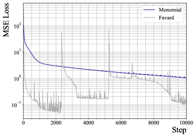
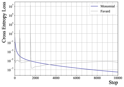
Figure 2: Drop of loss in 10,000 epochs. Left: MSE loss of regression task on one sample. Right: Cross entropy loss of classification problem on the Chameleon dataset. Models based on Monomial basis converge slowly, but stably. while FavardGNNs don’t converge. For the convergence curve for OptBasis, please check Figure 1. It converges much faster than Monomial Basis.

6 Conclusion

In this paper, we tackle the fundamental challenges of basis learning and computation in polynomial filters. We propose two models: FavardGNN and OptBasisGNN. FavardGNN learns arbitrary basis from the whole space of orthonormal polynomials, which is rooted in classical theorems in orthonormal polynomials. OptBasisGNN leverages the optimal basis defined by Wang & Zhang (2022) efficiently, which was thought unsolvable. Extensive experiments are conducted to demonstrate the effectiveness of our proposed models. An interesting future direction is to derive a convex and easier-to-optimize algorithm for FavardGNN.

Appendix A Notations

Table 6: Summation of notations in this paper.

Notation	Description
$G=(V,E)$	Undirected, connected graph
$N$	Number of nodes in $G$
$\hat{P}$	Symmetric-normalized adjacency matrix of $G$.
$\hat{L}$	Normalized Laplacian matrix of $G$. $\hat{L}$ = $I-\hat{P}$.
$\lambda_{i}$	The $i$-th eigenvalue of $\hat{L}$.
$\mu_{i}$	The $i$-th eigenvalue of $\hat{P}$. $\mu_{i}=1-\lambda_{i}.$
$U$	Eigen vectors of $\hat{L}$ and $\hat{P}$.
$x$	Input signal on $1$ channel.
$X\in\mathbb{R}^{N\times d}$	Input features / Input signals on $d$ channels.
$Z\in\mathbb{R}^{N\times d}$	Filtered signals.
$h(\cdot),$ $b(\cdot)$	Filtering function defined on $\hat{L}$ and $\hat{P}$, respectively. $h(\lambda)\equiv b(1-\lambda).$
$h_{i}(\cdot)$, $b_{i}(\cdot)$	Filtering function on the $i$th signal channel. $X_{i,:}=h_{i}(\hat{L})Z_{i,:}$.
$h(\hat{L})x,$ $b(\hat{P})x$	Filtering operation on signal $x$. $h(\hat{L})\equiv b(\hat{P})$.
$\{g_{k}(\cdot)\}_{k=0}^{K}$	A polynomial basis of truncated order $K$.
$\{\alpha_{k}\}_{k=0}^{K}$	Coefficients above a basis. i.e. $h(\lambda)\approx\sum_{k=0}^{K}\alpha_{k}g_{k}(\lambda).$

Appendix B Proofs

Most subsections here are for the convenience of interested readers. We provided our proofs about the theorems (except for the original form of Favard’s Theorem) and their relations used across our paper, although the theorems can be found in early chapters of monographs about orthogonal polynomials (Gautschi, 2004; Simon, 2014). We assume a relatively minimal prior background in orthogonal polynomials.

B.1 Three-term Recurrences for Orthogonal Polynomials (With Proof)

Theorem B.1 (Three-term Recurrences for Orthogonal Polynomials).

(Simon, 2005, p. 12) For any orthogonal polynomial series $\{p_{k}(x)\}_{k=0}^{\infty}$, suppose that the leading coefficients of all polynomial are positive, the series satisfies the recurrence relation:

$$p_{k+1}(x)=(A_{k}x+B_{k})p_{k}(x)+C_{k}p_{k-1}(x),$$

$$p_{-1}(x):=0,A_{k},C_{k}\in\mathbb{R}^{+},\ B_{k}\in\mathbb{R},\ k\geq 0.$$

Proof.

The core part of this proof is that $xp_{k}$ is orthogonal to $p_{i}$ for $i\leq k-2$, i.e.

$$\langle xp_{k},p_{i}\rangle=0,\quad i\leq k-2.$$

Since $xp_{k}(x)$ is of order $k+1$, we can rewrite $xp_{k}(x)$ into the combination of first $k+1$ polynomials of the basis:

$$xp_{k}(x)=\alpha_{k,k+1}p_{k+1}(x)+\alpha_{k,k}p_{k}(x)+a_{k,k-1}p_{k-1}(x)+\cdots+\alpha_{k,0}p_{0}(x)$$ (8)

or in short,

$$xp_{k}(x)=\sum_{j=k+1}^{0}\alpha_{k,j}p_{j}(x).$$

Project each term onto $p_{i}(x)$,

$$\langle xp_{k}(x),p_{i}(x)\rangle=\sum_{j=k+1}^{0}\alpha_{k,j}\langle p_{j}(x),p_{i}(x)\rangle.$$

Using the orthogonality among $\{p_{k}(x)\}_{k=0}^{\infty}$, we have

$$\langle xp_{k}(x),p_{i}(x)\rangle=\langle\alpha_{k,i}p_{i}(x),p_{i}(x)\rangle\Rightarrow\alpha_{k,i}=\frac{\langle xp_{k}(x),p_{i}(x)\rangle}{\langle p_{i}(x),p_{i}(x)\rangle}.$$ (9)

Next, we show $\langle xp_{k}(x),p_{i}(x)\rangle=0$ when $i\leq k-2$. Since $\langle xp_{k}(x),p_{i}(x)\rangle\equiv\langle p_{k}(x),xp_{i}(x)\rangle$, it is equivalent to show $\langle p_{k}(x),xp_{i}(x)\rangle=0$.

When $i\leq k-2$, applying $xp_{i}(x)=\sum_{j=0}^{i+1}\alpha_{i,j}p_{j}(x)$ and the orthogonality between $p_{j}(x)$ and $p_{k}(x)$ when $j\neq k$, we get

$$\langle p_{k},xp_{i}(x)\rangle=\sum_{j=0}^{i+1}\alpha_{i,j}\langle p_{k},p_{j}(x)\rangle\mathop{=}\limits^{j\leq k-1}0\Rightarrow\langle xp_{k},p_{i}(x)\rangle=0.$$

Therefore, $xp_{k}(x)$is only relevant to $p_{k+1}(x)$, $p_{k}(x)$ and $p_{k-1}(x)$. By shifting items, we soonly get that: $p_{k+1}(x)$is only relevant to $xp_{k}(x)$, $p_{k}(x)$ and $p_{k-1}(x)$.

At last, we show that, by regularizing the leading coefficients $A_{k}$ to be positive, ${C_{k}}>0$. Firstly, since the leading coefficients are positive, $\{\alpha_{k}\}_{k=0}^{\infty}$ defined in Equation (8) are positive. Then, notice from Equation (9), we get

$$-\frac{C_{k}}{A_{k}}=\alpha_{k,k-1}=\frac{\langle xp_{k}(x),p_{k-1}(x)\rangle}{\langle p_{k-1}(x),p_{k-1}(x)\rangle}=\frac{\langle p_{k}(x),xp_{k-1}(x)\rangle}{\langle p_{k-1}(x),p_{k-1}(x)\rangle}=\frac{\alpha_{k-1,k}}{\langle p_{k-1}(x),p_{k-1}(x)\rangle}.$$

We have finished our proof. ∎

B.2 Favard’s Theorem (Monomial Case)

Theorem B.2 (Favard’s Theorem).

(Favard, 1935) If a sequence of monic polynomials $\{P_{n}\}_{n=0}^{\infty}$ satisfies a three-term recurrence relation

$$P_{n+1}(x)=\left({x-\gamma_{n}}\right)P_{n}(x)-\beta_{n}P_{n-1}(x),$$

with $\gamma_{n},\beta_{n}\in\mathbb{R},\beta_{n}>0$, then $\{P_{n}\}_{n=0}^{\infty}$ is orthogonal with respect to some positive weight function.

B.3 Favard’s Theorem (General Case) (With Proof)

Corollary B.3 (Favard’s Theorem; general case).

If a sequence of polynomials $\{P_{n}\}_{n}^{\infty}$ statisfies a three-term recurrence relation

$$P_{n+1}(x)=\left(\varsigma_{n}{x-\gamma_{n}}\right)P_{n}(x)-\beta_{n}P_{n-1}(x),$$

with $\gamma_{n},\beta_{n},\varsigma_{n}\in\mathbb{R},\varsigma_{n}\neq 0,\beta_{n}/\varsigma_{n}>0$, then there exists a positive weight function $w$ such that $\{P_{n}\}_{n=0}^{\infty}$ is orthogonal with respect to the inner product $\langle p,q\rangle=\int_{\mathbb{R}}p(x)q(x)w(x)\mathrm{d}x$.

Proof.

Set $\gamma_{n}^{\ast}=\frac{\alpha_{n}}{\varsigma_{n}},\beta_{n}^{\ast}=\frac{\beta_{n}}{\varsigma_{n}}$. Then we can construct a sequence of polynomials $\{P_{n}^{\ast}\}_{n}^{\infty}$.

Case 1: For $n=0$ and $n=1$, set $P_{n}^{\ast}:=P_{n}(x)/\hat{P_{n}}(x)$ .

Case 2: For $n\geq 2$, define $P_{n}^{\ast}(x)$ by the three-term recurrences:

$$P_{n+1}^{\ast}(x):=\left({x-\gamma_{n}^{\ast}}\right)P_{n}^{\ast}(x)-\beta_{n}^{\ast}P_{n-1}^{\ast}(x).$$

According to Theorem B.2, $\{P_{n}^{\ast}\}_{n}$ is an orthogonal basis. Since $P_{n}$ is scaled $P_{n}^{\ast}$ by some constant, so $\{P_{n}\}_{n}$  is also orthogonal. ∎

B.4 Proof of Theorem 3.1

We restate the Theorem of three-term recurrences for orthonormal polynomials (Theorem 3.1) as below, and give a proof.

(Three Term Recurrences for Orthonormal Polynomials) For orthonormal polynomials $\{p_{k}\}_{k=0}^{\infty}$ w.r.t. weight function $w$, suppose that the leading coefficients of all polynomial are positive, there exists the three-term recurrence relation:

$$\sqrt{\beta_{k+1}}p_{k+1}(x)=(x-\gamma_{k})p_{k}(x)-\sqrt{\beta_{k}}p_{k-1}(x),$$

$$p_{-1}(x):=0,\ p_{0}(x)=1/\sqrt{\beta_{0}},\ \gamma_{k}\in\mathbb{R},\ \sqrt{\beta_{k}}\in\mathbb{R}^{+},\ k\geq 0$$

with $\beta_{0}=\int w(x)\mathrm{d}x$.

Proof.

Case 1: $k=0$. $p_{k}(x)$ is a constant. Suppose it to be $t$, then

$$\text{}\langle p_{0}(x),p_{0}(x)\rangle=t^{2}\int_{a}^{b}\hskip 1.69998pt\mathrm{d}\alpha\Rightarrow t=1/\sqrt{\beta_{0}}.$$

Case 2: $k\geq 1$. By Theorem B.1, since $\{p_{k}\}_{k=0}^{K}$ is orthogonal, there exist three term recurrences as such:

$$p_{k+1}(x)=(A_{k}x+B_{k})p_{k}(x)+C_{k}p_{k-1}(x),\quad k=1,2,3,\ldots.$$

By setting $c_{k}^{\ast}=\dfrac{1}{A_{k}}$, $a_{k}^{\ast}=-\dfrac{B_{k}}{A_{k}}$, $b_{k}^{\ast}=-\dfrac{{C_{k}}}{A_{k}}$, it can be rewritten into

$$c_{k}^{\ast}p_{k+1}(x)=(x-a_{k}^{\ast})p_{k}(x)-b_{k}^{\ast}p_{k-1}(x),\quad k=1,2,3,\ldots.$$ (10)

Apply dot products with $p_{k-1}(x)$ to Equation (10), we get

$$\langle xp_{k}(x),p_{k-1}(x)\rangle = \langle b^{\ast}_{k}p_{k-1}(x),p_{k-1}(x)\rangle$$

$$\Rightarrow b^{\ast}_{k}=\langle xp_{k}(x),p_{k-1}(x)\rangle$$

$$(k=1,2,3,\ldots).$$

Similarly, apply dot products with $p_{k+1}(x)$, we get:

$$\langle c_{k}^{\ast}p_{k+1}(x),p_{k+1}(x)\rangle = \langle xp_{k}(x),p_{k+1}(x)\rangle$$

$$\Rightarrow c_{k}^{\ast}=\langle xp_{k}(x),p_{k+1}(x)\rangle$$

$$\Rightarrow c_{k}^{\ast}=\langle xp_{k+1}(x),p_{k}(x)\rangle$$

$$(k=1,2,3,\ldots).$$

Notice that in Equation (B.4)

$$\langle xp_{k}(x),p_{k+1}(x)\rangle=\langle p_{k}(x),xp_{k+1}(x)\rangle\overset{\eqref{eq:proof_for_3term_ortho_medium_1}}{=}b_{k+1}^{\ast}.$$

We get:

$$c_{k}^{\ast}=b_{k+1}^{\ast}.$$

So we can write Equation (10) into the form below:

$$b_{k+1}^{\ast}p_{k+1}(x)=(x-a_{k}^{\ast})p_{k}(x)-b_{k}^{\ast}p_{k-1}(x),\quad k=1,2,3,\ldots.$$

At last, we show $b_{k}^{\ast}>0$.

Firstly, recall that $b^{\ast}_{k}=\langle xp_{k}(x),p_{k-1}(x)\rangle=\langle p_{k}(x),xp_{k-1}(x)\rangle$. Since $xp_{k-1}(x)$, which is of order $k$, can be written into the combination of $\{p_{j}\}_{j=0}^{k}$ which the leading coefficients to be non-zero, i.e.

$$xp_{k-1}(x)=a_{k,k}p_{k}(x)+a_{k,k-1}p_{k-1}(x)+\cdots+a_{k,0}p_{0}(x)\quad(a_{k,k}\neq 0)$$

Secondly, since $\langle g(x),g(x)\rangle\equiv\langle-g(x),-g(x)\rangle$, we can restrict all the leading coefficients to be positive.

$$b_{n}^{\ast}=\langle p_{k}(x),xp_{k-1}(x)\rangle=a_{k,k}>0.$$

Thus we have proved $b^{\ast}_{k}>0$ holds.

Furthermore, we can rewrite $b_{k}^{\ast}$ into $\sqrt{\beta_{k}}$. The proof is finished. ∎

B.5 Proof of Theorem 3.2

We restate Favard’s Theorem for orthonormal polynomials (Theorem 3.2) as below, and give a proof based on the general case B.3.

(Favard Theorem; Orthonormal case) A polynomial series $\{p_{k}\}_{k=0}^{\infty}$ who satisfies the recurrence relation

$$\sqrt{\beta_{k+1}}p_{k+1}(x)=(x-\gamma_{k})p_{k}(x)-\sqrt{\beta_{k}}p_{k-1}(x),$$

$$p_{-1}(x):=0,\ p_{0}(x)=1/\sqrt{\beta_{0}},\gamma_{k}\in\mathbb{R},\ \sqrt{\beta_{k}}\in\mathbb{R}^{+},\ k\geq 0$$

is orthonormal w.r.t. a weight function $w$ that $\beta_{0}=\int w(x)\mathrm{d}x$.

Proof.

First of all, according to Theorem 3.2, the series $\{p_{k}\}_{k=0}^{\infty}$ is orthogonal.

Apply dot products with $p_{k-1}(x)$, we get

$$\langle xp_{k}(x),p_{k-1}(x)\rangle = \left\langle\sqrt{\beta_{k}}p_{k-1}(x),p_{k-1}(x)\right\rangle$$

$$\Rightarrow\langle xp_{k}(x),p_{k-1}(x)\rangle = \sqrt{\beta_{k}}\langle p_{k-1}(x),p_{k-1}(x)\rangle$$

$$(k=0,1,\ldots).$$

Similarily, apply dot products with $p_{k+1}(x)$, we get:

$$\left\langle\sqrt{\beta_{k+1}}p_{k+1}(x),p_{k+1}(x)\right\rangle = \langle xp_{k}(x),p_{k+1}(x)\rangle$$

$$\Rightarrow\sqrt{\beta_{k+1}}\langle p_{k+1}(x),p_{k+1}(x)\rangle = \langle xp_{k}(x),p_{k+1}(x)\rangle$$

$$(k=0,1,\ldots),$$

which can be rewritten as:

$$\begin{array}[]{lll}\sqrt{\beta_{k}}\langle p_{k}(x),p_{k}(x)\rangle&=&\langle xp_{k-1}(x),p_{k}(x)\rangle\\ &&(k=1,2,\ldots),\end{array}$$

Notice that

$$\langle xp_{k-1}(x),p_{k}(x)\rangle=\langle xp_{k}(x),p_{k-1}(x)\rangle.$$

We get:

$$\sqrt{\beta_{k}}\langle p_{k}(x),p_{k}(x)\rangle = \langle xp_{k-1}(x),p_{k}(x)\rangle$$

$$= \sqrt{\beta_{k}}\langle p_{k-1}(x),p_{k-1}(x)\rangle$$

$$\Rightarrow\langle p_{k}(x),p_{k}(x)\rangle = \langle p_{k-1}(x),p_{k-1}(x)\rangle$$

$$(k=1,2,\ldots),$$

which indicates that the polynomials $\{p_{k}\}_{k=0}^{K}$ are same in their norm.

Since $p_{0}(x)\equiv 1/\sqrt{\beta_{0}}$ and $\beta_{0}=\int w(x)\mathrm{d}x$, $\left\langle{p_{0}}(x),p_{0}(x)\right\rangle=\dfrac{1}{{\beta_{0}}}\int w(x)\mathrm{d}x$ =1. Thus the norm of every polynomial in $\{p_{k}\}_{k=0}^{\infty}$ equals $1$.

Combining that $\{p_{k}\}_{k=0}^{\infty}$ is orthogonal and $\left\langle{p_{k}}(x),p_{k}(x)\right\rangle=1$ for all $k$, we arrive that $\{p_{k}\}_{k=0}^{\infty}$ is an orthonormal basis. ∎

B.6 Proof of Proposition 4.4

Proof.

First, from the construction of each $v_{i+1}$ (Algorithm 4, $k=i$), we know that $v_{i+1}$ is composed of $\{v_{j}\}_{j}^{j=i}$ and $\hat{P}v_{i}$. Therefore, $\hat{P}v_{i}$ can be expressed as a weighted sum of $\{v_{j}\}_{j=0}^{i+1}$, denoted as $\hat{P}v_{i}=t_{i+1}v_{i+1}+t_{i}v_{i}+\cdots+t_{0}v_{0}~{}(13)$. Second, notice that $\langle\hat{P}v_{k},v_{i}\rangle=v_{k}^{T}\hat{P}v_{i}=\langle v_{k},\hat{P}v_{i}\rangle~{}(14)$. Thus, for Step 2 in Algorithm 4, for each $i\in\left[0,1,\cdots,k\right]$ we can rephrase $\langle v_{k+1}^{*},v_{i}\rangle$ by:

$$\langle v_{k+1}^{*},v_{i}\rangle \overset{\text{def}}{=}\langle\hat{P}v_{k},v_{i}\rangle\overset{\eqref{eq:sym}}{=}\langle v_{k},\hat{P}v_{i}\rangle$$

$$\overset{\eqref{eq:weightsum}}{=}\left\langle v_{k},\sum_{j=0}^{i+1}t_{j}v_{j}\right\rangle$$

$$=\sum_{j=0}^{i+1}t_{j}\langle v_{k},v_{j}\rangle,$$

which equals $0$ when $i<k-1$. ∎

B.7 Proof of Lemma 4.6

Proof.

First, notice that

$$\langle v_{k+1}^{\ast},v_{k-1}\rangle=\langle\hat{P}v_{k},v_{k-1}\rangle=\langle v_{k},\hat{P}v_{k-1}\rangle.$$

On the other hand,

$$\|v_{k+1}^{\bot}\|=\langle v_{k+1},v_{k+1}^{\bot}\rangle=\langle v_{k+1},v_{k+1}^{\ast}\rangle=\langle v_{k+1},\hat{P}v_{k}\rangle.$$

So, we get

$$\|v^{\bot}_{k}\|=\langle v_{k},\hat{P}v_{k-1}\rangle=\langle\hat{P}v_{k},v_{k-1}\rangle=\langle v_{k+1}^{\ast},v_{k-1}\rangle.$$

∎

Thus, we have finished our proof.

Appendix C Pseudo-codes

C.1 Pseudo-code for FavardGNN.

⬇

# f: raw feature dimension

# d: hidden dimension, or number of channels

# N: number of nodes

# K: order of polynomial basis

# X(Nxd): Input features

# P(NxN): Sym-normalized adjacency matrix

# Coef(dx(K+1)): coefficient matrix

# SqrtBeta(dx(K+1)): Coefficients for three-term recurrences

# Gamma(dx(K+1)): Coefficients for three-term recurrences

# Transfer raw input in signals

X = ReLU(MLP(X.dropout())).dropout() # (Nxd)

SqrtBeta = torch.clamp(norm, 1e-2)

# Process H_0

H_0 = X / SqrtBeta[:,0] # (Nxd)

Z = torch.zeros_like(X)

# Add to the final representation

Z = Z + torch.einsum(’Nd,d->Nd’, H_0, Coef[:,0])

last_H = H_0

second_last_H = torch.zeros_like(H_0)

for k in range(1, K):

# Three-term Recurrence Formula for Orthonormal Polynomials

H_k = P @ last_H # (Nxd)

H_k = H_k - Gamma[k,:].unsqueeze(0)*last_H - SqrtBeta[k,:].unsqueeze(0)*second_last_H

H_k = H_k / SqrtBeta[k+1,:].unsqueeze(0)

# Add to the final representation

Z = Z + torch.einsum(’Nd,d->Nd’, H_k, Coef[:,k])

# Update variables

second_last_H = last_H

last_H = H_k

# Transform the final representation into predictions

Y = MLP(ReLU(Z).dropout())

Pred = Softmax(Y)

return Pred

 

Algorithm 7 FavardGNN.Pytorch style.

C.2 Pseudo-code for OptBasisGNN.

1

⬇

# f: raw feature dimension

# d: hidden dimension, or number of channels

# N: number of nodes

# K: order of polynomial basis

# X(Nxd): Input features

# P(NxN): Sym-normalized adjacency matrix

# Coef(dxK): coefficient matrix

# Transfer raw input in signals

X = ReLU(MLP(X.dropout())).dropout() # (Nxd)

# Normalize H_0

norm = torch.norm(X, dim=0).view(1, d)

norm = torch.clamp(norm, 1e-8)

H_0 = X / norm # (Nxd)

Z = torch.zeros_like(X)

# Add to the final representation

Z = Z + torch.einsum(’Nd,d->Nd’, H_0, Coef[:,0])

last_H = H_0

second_last_H = torch.zeros_like(H_0)

for k in range(1, K):

H_k = P @ last_H # (Nxd)

# Orthogonalize H_k to all the former vectors

# To achieve this, only 2 substractions are required

project_1 = torch.einsum(’Nd,Nd->1d’, H_k, last_H) # (1xd)

project_2 = torch.einsum(’Nd,Nd->1d’, H_k, second_last_H) # (1xd)

H_k = H_k - project_1 * last_H - project_2 * second_last_H # (Nxd)

# Normalize H_k

norm = torch.norm(H_k, dim=0).view(1, d)

norm = torch.clamp(norm, 1e-8)

H_k = H_k / norm # (Nxd)

# Add to the final representation

Z = Z + torch.einsum(’Nd,d->Nd’, H_k, Coef[:,k])

# Update variables

second_last_H = last_H

last_H = H_k

# Transform the final representation to predictions

Y = MLP(ReLU(Z).dropout())

Pred = Softmax(Y)

return Pred

 

Algorithm 8 OptBasisGNN.Pytorch style.

Appendix D Experimental Settings.

D.1 Node Classification Tasks on Large and Small Datasets.

Model setup.

The structure of FavardGNN and OptBasisGNN follow Algorithm 2. The hidden size of the first MLP layers $h$ is set to be $64$, which is also the number of filter channels. For the scaled-up OptBasisGNN, we drop the first MLP layer to fix the basis vectors needed for precomputing, and following the scaled-up version of ChebNetII (He et al., 2022), we add a three-layer MLP with weight matrices of shape $F\times h$, $h\times h$ and $h\times c$ after the filtering process.

For both models, the initialization of $\alpha$ is set as follows: for each channel $l$, the coefficients of the $g_{0,l}$ are set to be $1$, while the other coefficients are set as zeros, which corresponds to initializing the polynomial filter on each channel to be $h(\lambda)=1-\lambda$. For the initialization of three-term parameters that determine the initial polynomial bases on each channel, we simply set $\{\sqrt{\beta}\}$ to be ones, and $\{\gamma\}$ to be zeros.

Hyperparameter tunning.

For the optimization process on the training sets, we tune all the parameters with Adam  (Kingma & Ba, 2015) optimizer. We use early stopping with a patience of 300 epochs.

We choose hyperparameters on the validation sets. To accelerate hyperparameter choosing, we use Optuna(Akiba et al., 2019) to select hyperparameters from the range below with a maximum of 100 complete trials:

1. Truncated Order polynomial series: $K\in\{2,4,8,12,16,20\}$;

2. Learning rates: $\{0.0005,0.001,0.005,0.1,0.2,0.3,0.4,0.5\}$;

3. Weight decays: $\{1\mathrm{e}{-8},\cdots,1\mathrm{e}{-3}\}$;

4. Dropout rates: $\{0.,0.1,\cdots,0.9\}$;

There are two extra hyperparameters for scaled-up OptBasisGNN:

1. Batch size: $\{10,000,50,000\}$;

2. Hidden size (for the post-filtering MLP): $\{512,1024,2048\}$.

D.2 Multi-Channel Filter Learning Task.

YCbCr Channels.

We put the practical background of our multichannel experiment in the YCbCr color space, a useful color space in computer vision and multi-media  (Shaik et al., 2015).

Our Synthetic Dataset.

When creating our datasets with 60 samples, we use 4 filter combinations on 15 images in He et al. (2021)’s single filter learning datasets. The 4 combinations on the three channels are:

1. Band-reject(Y) / low-pass(Cb) / high-pass(Cr);

2. High-pass(Y) / High-pass(Cb) / low-pass(Cr);

3. High-pass(Y) / low-pass(Cb) / High-pass(Cr);

4. Low-pass(Y) / band-reject(Cb) / band-reject(Cr).

The concrete definitions of the signals, i.e. band-reject are aligned with those given in He et al. (2022).

Visualization on more samples.

We visualize more samples as Figure 1 in Figure 3. In all the samples, the tendencies of different curves are alike.

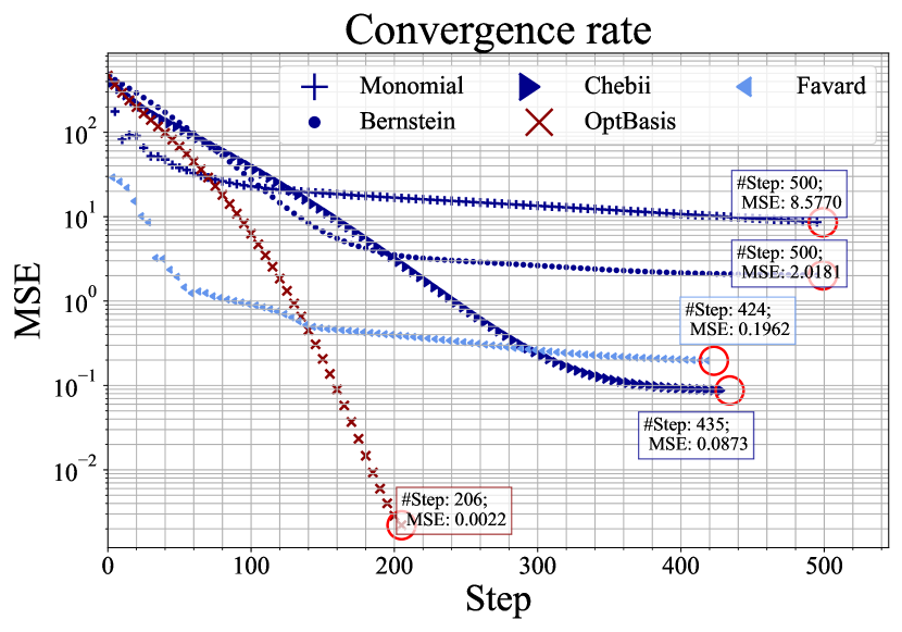
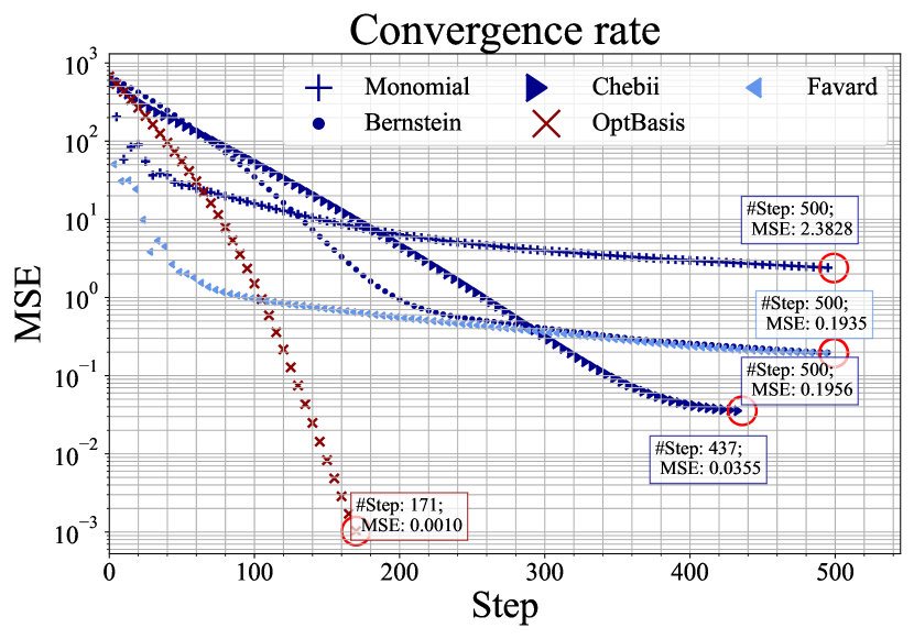
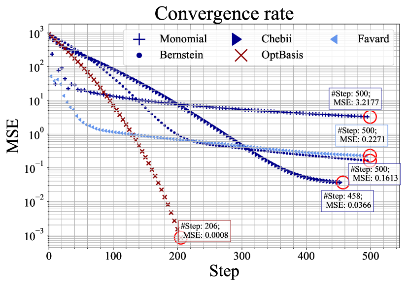
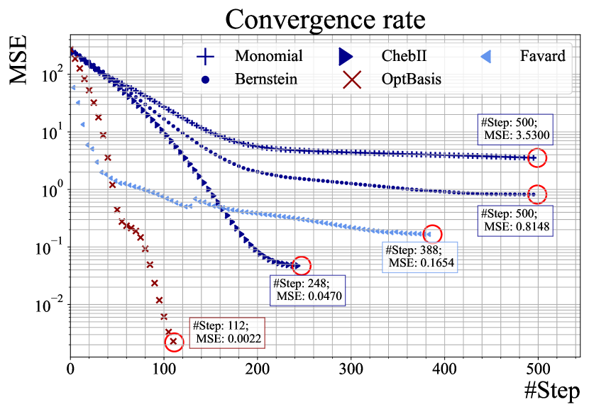
Figure 3: Visualization with more samples in the multi-channel filter learning task.

D.3 Examining of FavardGNN’s bump.

Figure 2 (right), we observe bump with a node classification setup. To show this clearer, we let FavardGNN and GPR-GNN (which uses the Monomial basis for classification) to fit the whole set of nodes, and move dropout and Relu layers. As in the regression re-examine task, we cancel the earlystop mechanism, stretch the epoch number to 10,000, and record cross entropy loss on each epoch.

Appendix E Summary of Wang’s work

This section is a restate for a part of Wang & Zhang (2022). For the convenience of the reader’s reference, we write this section here. More interested readers are encouraged to refer to the original paper.

Wang & Zhang (2022) raise a criterion for best basis, but states that it cannot be reached.

E.1 The Criterion for Optimal Basis

Following Xu et al. (2021), Wang & Zhang (2022) considers the squared loss $R=\frac{1}{2}\|Z-Y\|_{\textrm{F}}^{2}$, where $Y$ is the target , and $Z=\underset{l\in[1,h]}{\|}\sum_{k=0}^{K}\alpha_{k,l}g_{k,l}(\hat{P})X_{:,l}$ .

Since each signal channel is independent and contributes independently to the loss, i.e. $R=\sum_{l}\frac{1}{2}\|Z_{:,l}-Y_{:,l}\|_{\mathrm{F}}^{2}$, we can then consider the loss function channelwisely and ignore $l$. Loss on one signal channel $x$ is:

$$r=\frac{1}{2}\|z-y\|^{2}_{\textrm{F}},$$

where $z=\sum_{k=0}^{K}\alpha_{k}g_{k}(\hat{P})x$.

This loss is a convex function w.r.t. $\alpha$. Therefore, the gradient descents’s convergence rate depends on the Hessian matrix’s condition number, denoted as $\kappa(H)$. When $H$ is an identity matrix, $\kappa(H)$ reaches a minimum and leads to the best convergence rate (Boyd & Vandenberghe, 2009).

The Hessian matrix $H$ looks like:

$$H_{k_{1}k_{2}}=\frac{\partial^{2}r}{\partial\alpha_{k_{1}}\partial\alpha_{k_{2}}}=x^{\mathrm{T}}g_{k_{2}}(\hat{P})g_{k_{1}}(\hat{P})x.$$

Wang & Zhang (2022) further write $H_{k_{1}k_{2}}$ in the following form:

$$H_{k_{1}k_{2}}=x^{T}g_{k_{2}}(\hat{P})g_{k_{1}}(\hat{P})x=\sum_{i=1}^{n}g_{k_{1}}(\mu_{i})g_{k_{2}}(\mu_{i})(U^{\mathrm{T}}x)_{i}^{2},$$

which can be equivalently expressed as a Riemann sum:

$$\sum^{N}_{i=1}g_{k_{1}}(\mu_{i})g_{k_{2}}(\mu_{i})\frac{F(\mu_{i})-F(\mu_{i-1})}{\mu_{i}-\mu_{i-1}}(\mu_{i}-\mu_{i-1}),$$

where $F(\mu):=\sum_{\mu_{i}\leq\mu}(U^{\mathrm{T}}x)_{i}^{2}$ . Define $f(\mu)=\frac{\vartriangle F(\mu)}{\vartriangle\mu}$, $H_{k_{1}k_{2}}$ comes to

$$H_{k_{1}k_{2}}=\text{}\int_{\mu=-1}^{1}g_{k_{1}}(\mu)g_{k_{2}}(\mu)f(\mu)\mathrm{d}\mu.$$

This suggests that, $\{g_{k}\}_{k=0}^{K}$ is an optimal basis when it is orthonormal w.r.t. weight function $f(\cdot)$. (For more about orthonormal basis, see Section 2.2.)

E.2 Wang’s Method

Having write out the weight function $f(\mu)$, the optimal basis is determined. Wang & Zhang (2022) think of a regular process for getting this optimal basis, which is unreachable since eigendecomposition is unaffordable for large graphs. We summarize this process in Algorithm 3.

According to Wang & Zhang (2022), the optimal basis would be an orthonormal basis, but unfortunately, this basis and the exact form of its weight function is unattainable. As a result, they come up with a compromise by allowing the model to choose from the orthogonal Jacobi bases, which have “flexible enough weight functions”, i.e. $(1-\mu)^{a}(1+\mu)^{b}$. The Jacobi bases are a family of polynomial bases. A specific form Jacobi basis is determined by two parameters $\left(a,b\right)$. Similar to the well-known Chebyshev basis, the Jacobi bases have a recursive formulation, making them efficient for calculation.

References

- Abu-El-Haija et al. (2019) Abu-El-Haija, S., Perozzi, B., Kapoor, A., Alipourfard, N., Lerman, K., Harutyunyan, H., Steeg, G. V., and Galstyan, A. Mixhop: Higher-order graph convolutional architectures via sparsified neighborhood mixing. In Chaudhuri, K. and Salakhutdinov, R. (eds.), Proceedings of the 36th International Conference on Machine Learning, ICML 2019, 9-15 June 2019, Long Beach, California, USA, volume 97 of Proceedings of Machine Learning Research, pp. 21–29. PMLR, 2019. URL http://proceedings.mlr.press/v97/abu-el-haija19a.html.
- Akiba et al. (2019) Akiba, T., Sano, S., Yanase, T., Ohta, T., and Koyama, M. Optuna: A next-generation hyperparameter optimization framework. In Teredesai, A., Kumar, V., Li, Y., Rosales, R., Terzi, E., and Karypis, G. (eds.), Proceedings of the 25th ACM SIGKDD International Conference on Knowledge Discovery & Data Mining, KDD 2019, Anchorage, AK, USA, August 4-8, 2019, pp. 2623–2631. ACM, 2019. doi: 10.1145/3292500.3330701. URL https://doi.org/10.1145/3292500.3330701.
- Balcilar et al. (2021) Balcilar, M., Renton, G., Héroux, P., Gaüzère, B., Adam, S., and Honeine, P. Analyzing the expressive power of graph neural networks in a spectral perspective. In 9th International Conference on Learning Representations, ICLR 2021, Virtual Event, Austria, May 3-7, 2021. OpenReview.net, 2021. URL https://openreview.net/forum?id=-qh0M9XWxnv.
- Bianchi et al. (2021) Bianchi, F. M., Grattarola, D., Livi, L., and Alippi, C. Graph neural networks with convolutional arma filters. IEEE transactions on pattern analysis and machine intelligence, 44(7):3496–3507, 2021.
- Chen et al. (2020a) Chen, M., Wei, Z., Ding, B., Li, Y., Yuan, Y., Du, X., and Wen, J. Scalable graph neural networks via bidirectional propagation. CoRR, abs/2010.15421, 2020a. URL https://arxiv.org/abs/2010.15421.
- Chen et al. (2020b) Chen, M., Wei, Z., Huang, Z., Ding, B., and Li, Y. Simple and deep graph convolutional networks. In Proceedings of the 37th International Conference on Machine Learning, ICML 2020, 13-18 July 2020, Virtual Event, volume 119 of Proceedings of Machine Learning Research, pp. 1725–1735. PMLR, 2020b. URL http://proceedings.mlr.press/v119/chen20v.html.
- Chien et al. (2021) Chien, E., Peng, J., Li, P., and Milenkovic, O. Adaptive universal generalized pagerank graph neural network. In 9th International Conference on Learning Representations, ICLR 2021, Virtual Event, Austria, May 3-7, 2021. OpenReview.net, 2021. URL https://openreview.net/forum?id=n6jl7fLxrP.
- Defferrard et al. (2016) Defferrard, M., Bresson, X., and Vandergheynst, P. Convolutional neural networks on graphs with fast localized spectral filtering. In Lee, D. D., Sugiyama, M., von Luxburg, U., Guyon, I., and Garnett, R. (eds.), Advances in Neural Information Processing Systems 29: Annual Conference on Neural Information Processing Systems 2016, December 5-10, 2016, Barcelona, Spain, pp. 3837–3845, 2016. URL https://proceedings.neurips.cc/paper/2016/hash/04df4d434d481c5bb723be1b6df1ee65-Abstract.html.
- Favard (1935) Favard, J. Sur les polynomes de tchebicheff. CR Acad. Sci. Paris, 200(2052-2055):11, 1935.
- Frasca et al. (2020) Frasca, F., Rossi, E., Eynard, D., Chamberlain, B., Bronstein, M., and Monti, F. Sign: Scalable inception graph neural networks. In ICML 2020 Workshop on Graph Representation Learning and Beyond, 2020.
- Gautschi (2004) Gautschi, W. Orthogonal polynomials: computation and approximation. OUP Oxford, 2004.
- Geronimo & Van Assche (1991) Geronimo, J. and Van Assche, W. Approximating the weight function for orthogonal polynomials on several intervals. Journal of Approximation Theory, 65(3):341–371, 1991. ISSN 0021-9045. doi: https://doi.org/10.1016/0021-9045(91)90096-S. URL https://www.sciencedirect.com/science/article/pii/002190459190096S.
- Hammond et al. (2009) Hammond, D. K., Vandergheynst, P., and Gribonval, R. Wavelets on graphs via spectral graph theory. CoRR, abs/0912.3848, 2009. URL http://arxiv.org/abs/0912.3848.
- He et al. (2021) He, M., Wei, Z., Huang, Z., and Xu, H. Bernnet: Learning arbitrary graph spectral filters via bernstein approximation. In Ranzato, M., Beygelzimer, A., Dauphin, Y. N., Liang, P., and Vaughan, J. W. (eds.), Advances in Neural Information Processing Systems 34: Annual Conference on Neural Information Processing Systems 2021, NeurIPS 2021, December 6-14, 2021, virtual, pp. 14239–14251, 2021. URL https://proceedings.neurips.cc/paper/2021/hash/76f1cfd7754a6e4fc3281bcccb3d0902-Abstract.html.
- He et al. (2022) He, M., Wei, Z., and Wen, J.-R. Convolutional neural networks on graphs with chebyshev approximation, revisited. arXiv preprint arXiv:2202.03580, 2022.
- Hu et al. (2020) Hu, W., Fey, M., Zitnik, M., Dong, Y., Ren, H., Liu, B., Catasta, M., and Leskovec, J. Open graph benchmark: Datasets for machine learning on graphs. In Larochelle, H., Ranzato, M., Hadsell, R., Balcan, M., and Lin, H. (eds.), Advances in Neural Information Processing Systems 33: Annual Conference on Neural Information Processing Systems 2020, NeurIPS 2020, December 6-12, 2020, virtual, 2020. URL https://proceedings.neurips.cc/paper/2020/hash/fb60d411a5c5b72b2e7d3527cfc84fd0-Abstract.html.
- Isufi et al. (2021) Isufi, E., Gama, F., and Ribeiro, A. Edgenets: Edge varying graph neural networks. IEEE Transactions on Pattern Analysis and Machine Intelligence, 44(11):7457–7473, 2021.
- Isufi et al. (2022) Isufi, E., Gama, F., Shuman, D. I., and Segarra, S. Graph filters for signal processing and machine learning on graphs. arXiv preprint arXiv:2211.08854, 2022.
- Kingma & Ba (2015) Kingma, D. P. and Ba, J. Adam: A method for stochastic optimization. In Bengio, Y. and LeCun, Y. (eds.), 3rd International Conference on Learning Representations, ICLR 2015, San Diego, CA, USA, May 7-9, 2015, Conference Track Proceedings, 2015. URL http://arxiv.org/abs/1412.6980.
- Kipf & Welling (2017) Kipf, T. N. and Welling, M. Semi-supervised classification with graph convolutional networks. In 5th International Conference on Learning Representations, ICLR 2017, Toulon, France, April 24-26, 2017, Conference Track Proceedings. OpenReview.net, 2017. URL https://openreview.net/forum?id=SJU4ayYgl.
- Klicpera et al. (2019) Klicpera, J., Bojchevski, A., and Günnemann, S. Predict then propagate: Graph neural networks meet personalized pagerank. In 7th International Conference on Learning Representations, ICLR 2019, New Orleans, LA, USA, May 6-9, 2019. OpenReview.net, 2019. URL https://openreview.net/forum?id=H1gL-2A9Ym.
- Lim et al. (2021) Lim, D., Hohne, F., Li, X., Huang, S. L., Gupta, V., Bhalerao, O., and Lim, S. Large scale learning on non-homophilous graphs: New benchmarks and strong simple methods. In Ranzato, M., Beygelzimer, A., Dauphin, Y. N., Liang, P., and Vaughan, J. W. (eds.), Advances in Neural Information Processing Systems 34: Annual Conference on Neural Information Processing Systems 2021, NeurIPS 2021, December 6-14, 2021, virtual, pp. 20887–20902, 2021. URL https://proceedings.neurips.cc/paper/2021/hash/ae816a80e4c1c56caa2eb4e1819cbb2f-Abstract.html.
- Pei et al. (2020) Pei, H., Wei, B., Chang, K. C., Lei, Y., and Yang, B. Geom-gcn: Geometric graph convolutional networks. In 8th International Conference on Learning Representations, ICLR 2020, Addis Ababa, Ethiopia, April 26-30, 2020. OpenReview.net, 2020. URL https://openreview.net/forum?id=S1e2agrFvS.
- Sen et al. (2008) Sen, P., Namata, G., Bilgic, M., Getoor, L., Galligher, B., and Eliassi-Rad, T. Collective classification in network data. AI magazine, 29(3):93–93, 2008.
- Shaik et al. (2015) Shaik, K. B., Ganesan, P., Kalist, V., Sathish, B., and Jenitha, J. M. M. Comparative study of skin color detection and segmentation in hsv and ycbcr color space. Procedia Computer Science, 57:41–48, 2015.
- Shuman et al. (2013) Shuman, D. I., Ricaud, B., and Vandergheynst, P. Vertex-frequency analysis on graphs. CoRR, abs/1307.5708, 2013. URL http://arxiv.org/abs/1307.5708.
- Simon (2005) Simon, B. Orthogonal polynomials on the unit circle, part 1: Classical theory, ams colloq, 2005.
- Simon (2014) Simon, B. Spectral theory of orthogonal polynomials. In XVIIth International Congress on Mathematical Physics, pp. 217–228. World Scientific, 2014.
- Wang et al. (2019) Wang, G., Ying, R., Huang, J., and Leskovec, J. Improving graph attention networks with large margin-based constraints. CoRR, abs/1910.11945, 2019. URL http://arxiv.org/abs/1910.11945.
- Wang & Zhang (2022) Wang, X. and Zhang, M. How powerful are spectral graph neural networks. In Chaudhuri, K., Jegelka, S., Song, L., Szepesvári, C., Niu, G., and Sabato, S. (eds.), International Conference on Machine Learning, ICML 2022, 17-23 July 2022, Baltimore, Maryland, USA, volume 162 of Proceedings of Machine Learning Research, pp. 23341–23362. PMLR, 2022. URL https://proceedings.mlr.press/v162/wang22am.html.
- Wu et al. (2019) Wu, F., Zhang, T., Jr., A. H. S., Fifty, C., Yu, T., and Weinberger, K. Q. Simplifying graph convolutional networks. CoRR, abs/1902.07153, 2019. URL http://arxiv.org/abs/1902.07153.
- Xu et al. (2021) Xu, K., Zhang, M., Jegelka, S., and Kawaguchi, K. Optimization of graph neural networks: Implicit acceleration by skip connections and more depth. In Meila, M. and Zhang, T. (eds.), Proceedings of the 38th International Conference on Machine Learning, volume 139, pp. 11592–11602, 2021.
- Yang et al. (2016) Yang, Z., Cohen, W. W., and Salakhutdinov, R. Revisiting semi-supervised learning with graph embeddings. In Balcan, M. and Weinberger, K. Q. (eds.), Proceedings of the 33nd International Conference on Machine Learning, ICML 2016, New York City, NY, USA, June 19-24, 2016, volume 48 of JMLR Workshop and Conference Proceedings, pp. 40–48. JMLR.org, 2016. URL http://proceedings.mlr.press/v48/yanga16.html.
- Zhang et al. (2021) Zhang, W., Yang, M., Sheng, Z., Li, Y., Ouyang, W., Tao, Y., Yang, Z., and Cui, B. Node dependent local smoothing for scalable graph learning. Advances in Neural Information Processing Systems, 34:20321–20332, 2021.