An Oscillation-free Spectral Volume Method for Hyperbolic Conservation Laws

Abstract

In this paper, an oscillation-free spectral volume (OFSV) method is proposed and studied for the hyperbolic conservation laws. The numerical scheme is designed by introducing a damping term in the standard spectral volume method for the purpose of controlling spurious oscillations near discontinuities. Based on the construction of control volumes (CVs), two classes of OFSV schemes are presented. A mathematical proof is provided to show that the proposed OFSV is stable and has optimal convergence rate and some desired superconvergence properties when applied to the linear scalar equations. Both analysis and numerical experiments indicate that the damping term would not destroy the order of accuracy of the original SV scheme and can control the oscillations discontinuities effectively. Numerical experiments are presented to demonstrate the accuracy and robustness of our scheme.

65M08, 65M15, 65M60, 65N08

1 Introduction

The development of high-order schemes for hyperbolic conservation laws has becomes extremely demanding for computational fluid dynamics. In recent years, a great number high-order numerical schemes have been developed, including discontinuous Galerkin (DG) [1, 2, 3], spectral volume (SV) [5, 6, 7, 4], spectral difference (SD) [8], correction procedure using reconstruction (CPR) [9], essential non-oscillatory (ENO) [10, 11], weighted essential non-oscillatory (WENO) [12, 13, 14], Hermite WENO (HWENO) [15, 16, 17] methods, etc.

One main difficulty for the high-order numerical schemes is the spurious oscillations near discontinuities, which lead to the nonlinear instability and eventual blow up of the codes. Therefore, it is important to eliminate the oscillations near discontinuities and maintain the original high-order accuracy in the smooth regions. Many limiters have been studied in the literatures for DG methods. The minmod total variation bounded (TVB) limiter [2, 18, 19] was originally developed, which is a slope limiter using a technique from the finite volume method [20]. One disadvantage of such limiter is that it may degrade accuracy in smooth regions. The WENO reconstructions are also used as limiter for the DG methods [21, 22, 23]. In these methods, the WENO reconstructions were used to reconstruct the values at Gaussian quadrature points in the target cells, and rebuild the solution polynomials from the original cell average and the reconstructed values through a numerical integration. Although the original order of accuracy can be kept, the WENO limiters need a very large stencil, which is complicated to be implemented in multi-dimensions, especially for unstructured meshes. To use the compact stencils, the HWENO limiters are developed [15, 16, 17], which reduce the stencil of the reconstruction by utilizing both the cell averages and the spatial derivatives from the neighbors. The role of limiters is to “limit” and ”preprocess” numerical solution in the “troubled cells”, which is often identified by a troubled cell indicator. Another method is to add artificial diffusion terms in the weak formulation, which should be carefully designed to ensure entropy stability and suppress the oscillations essentially [24]. Recently, an oscillation-free DG (OFDG) method was developed for the scalar hyperbolic conservation laws in [25] by introducing a damping term on the classical DG scheme. The damping term was carefully constructed, which controls spurious nonphysical oscillations near discontinuities and maintains uniform high-order accuracy in smooth regions simultaneously. One advantage of the damping term was that the damping technique is convenient for the theoretical analysis, at least in the semi-discrete analysis, including conservation, $L^{2}$-stability, optimal error estimates, and even superconvergence. The OFDG has also been extended to the hyperbolic systems [26] and well-balanced shallow water equations [27].

The main purpose of the current work is to adopt the idea of damping term in [25] to the standard SV method for system of hyperbolic equations. The SV method was originally formulated and later developed for hyperbolic equations by Wang and his colleagues [5, 6, 7], which might be regarded as a generalization of the classic Godunov finite volume method [28, 29]. The SV method enjoys many excellent properties such as high-order accuracy, compact stencils, and geometrical flexibility (applicable for unstructured grids). In particular, since the SV method preserves conservation laws on more finer meshes, it might have a higher resolution for discontinuities than other high order methods (see [4]). During the past decades, the SV method has been rapidly applied to solving various PDEs such as the shallow water wave equation [30], Navier Stokes equation [31, 32], and electromagnetic field [5], and so on. A mathematical analysis in terms of the $L^{2}$ stability, accuracy, error estimates, and superconvergence of the SV method was conducted in [33] under the framework of the Petrov-Galerkin method. It was also proved in [33] that a special class of SV scheme is exactly the same as the upwind DG schemes when applied to linear constant hyperbolic equations.

By introducing the idea of damping term into the SV scheme, a new OFSV method is proposed in this article. The OFSV method inherits both advantages of the standard SV method and the damping term. Specifically, In one hand, properties such as high order accuracy, local conservation, $h$-$p$ adaptivity, flexibility of handling unstructured meshes can still be preserved for OFSV method. On the other hand, the OFSV method could effectively control spurious nonphysical oscillations near discontinuities and maintaining uniform high-order accuracy in smooth regions, without any use of limiters. Furthermore, note that the SV method has larger CFL condition number than the DG method (see, e.g., [34]), which suggests that the proposed OFSV method might have a looser stability condition than the counterpart OFDG method.

The rest of this paper is organized as follows. In Section 2, the OFSV method for systems of hyperbolic conservation laws is introduced. In Section 3, a theoretical analysis is provided to show that proposed OFSV method is stable and has optimal convergence rate and superconvergnce property similar to the standard SV method, when applied to for one-dimensional constant-coefficient linear scalar problem. In Section 4, we present some numerical examples to show the efficiency and robustness of our algorithm. Finally, some concluding remarks are presented in Section 5.

2 Oscillation-free SV method

We consider the OFSV method for the following hyperbolic system

(1) $$\left\{\begin{array}[]{l}\boldsymbol{U}_{t}+\displaystyle\sum_{i=1}^{d}\boldsymbol{F}_{i}(\boldsymbol{U})_{x_{i}}=0,\quad(\boldsymbol{x},t)\in\Omega\times(0,T],\\ \boldsymbol{U}(\boldsymbol{x},0)=\boldsymbol{U}_{0}(\boldsymbol{x}),\quad\boldsymbol{x}\in\Omega,\end{array}\right.$$

where $\boldsymbol{x}=(x_{1},\ldots,x_{d})^{T},$ $\boldsymbol{U}=(U_{1},\ldots,U_{m})^{T}$, $\boldsymbol{F}_{i}(\boldsymbol{U})=(F_{i,1}(\boldsymbol{U}),\ldots,F_{i,m}(\boldsymbol{U}))^{T},1\leq i\leq d$, and $\Omega$ is an open bounded domain in $\mathbb{R}^{d}$. A large amount of physical models can be rewritten into the form of (1), such as the Euler equations for the two-dimensional inviscid compressible flow, where $\boldsymbol{U}=\left(\rho,\rho U,\rho V,\rho E\right)$, $\boldsymbol{F}_{1}(\boldsymbol{U})=(\rho U,\rho U^{2}+p,\rho UV,(\rho E+p)U)$, $\boldsymbol{F}_{2}(\boldsymbol{U})=(\rho V,\rho UV,\rho V^{2}+p,(\rho E+p)V)$ with $\rho E=1/2\rho(U^{2}+V^{2})+p/(\gamma-1)$ for the two-dimensional ideal gas.

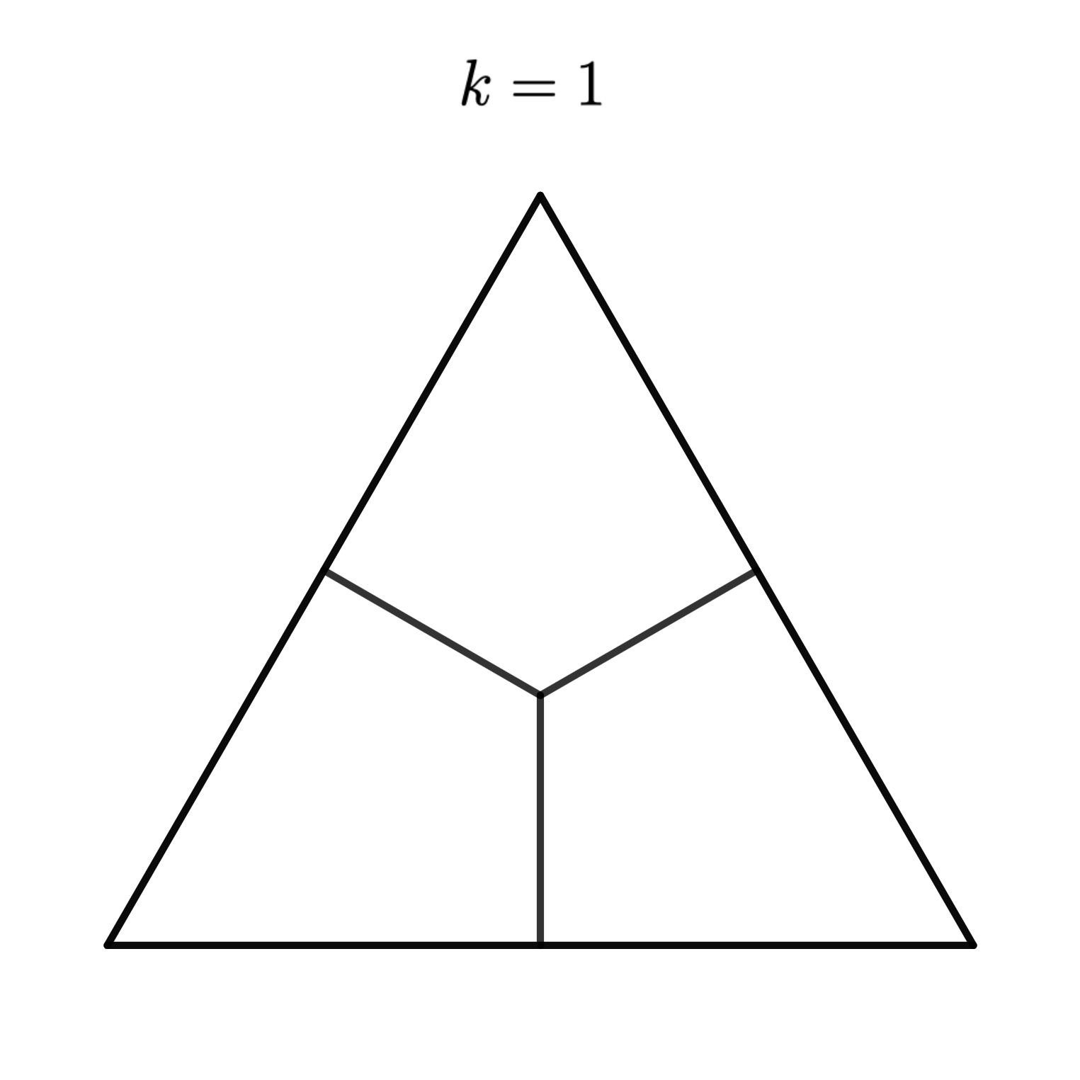
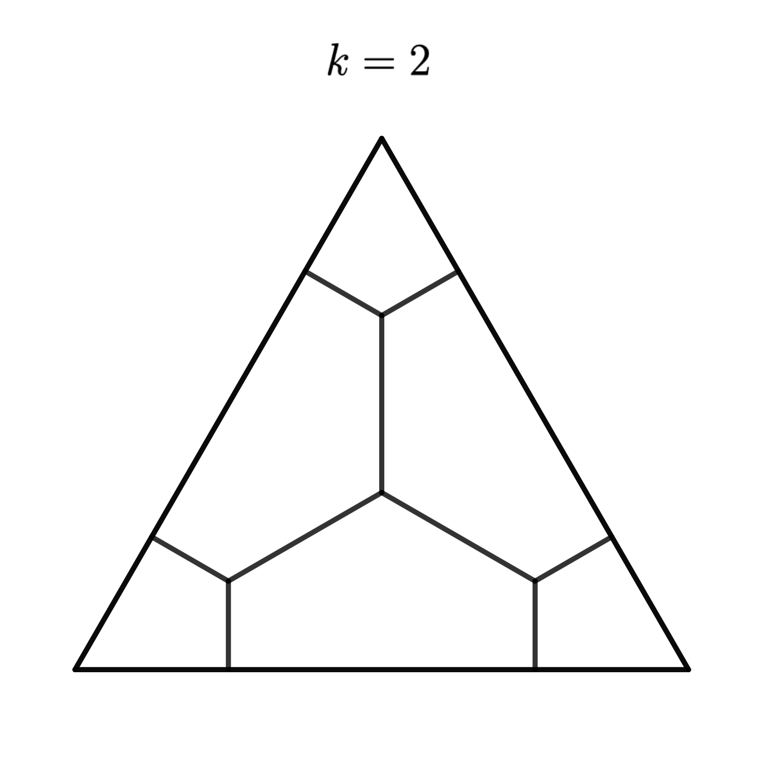
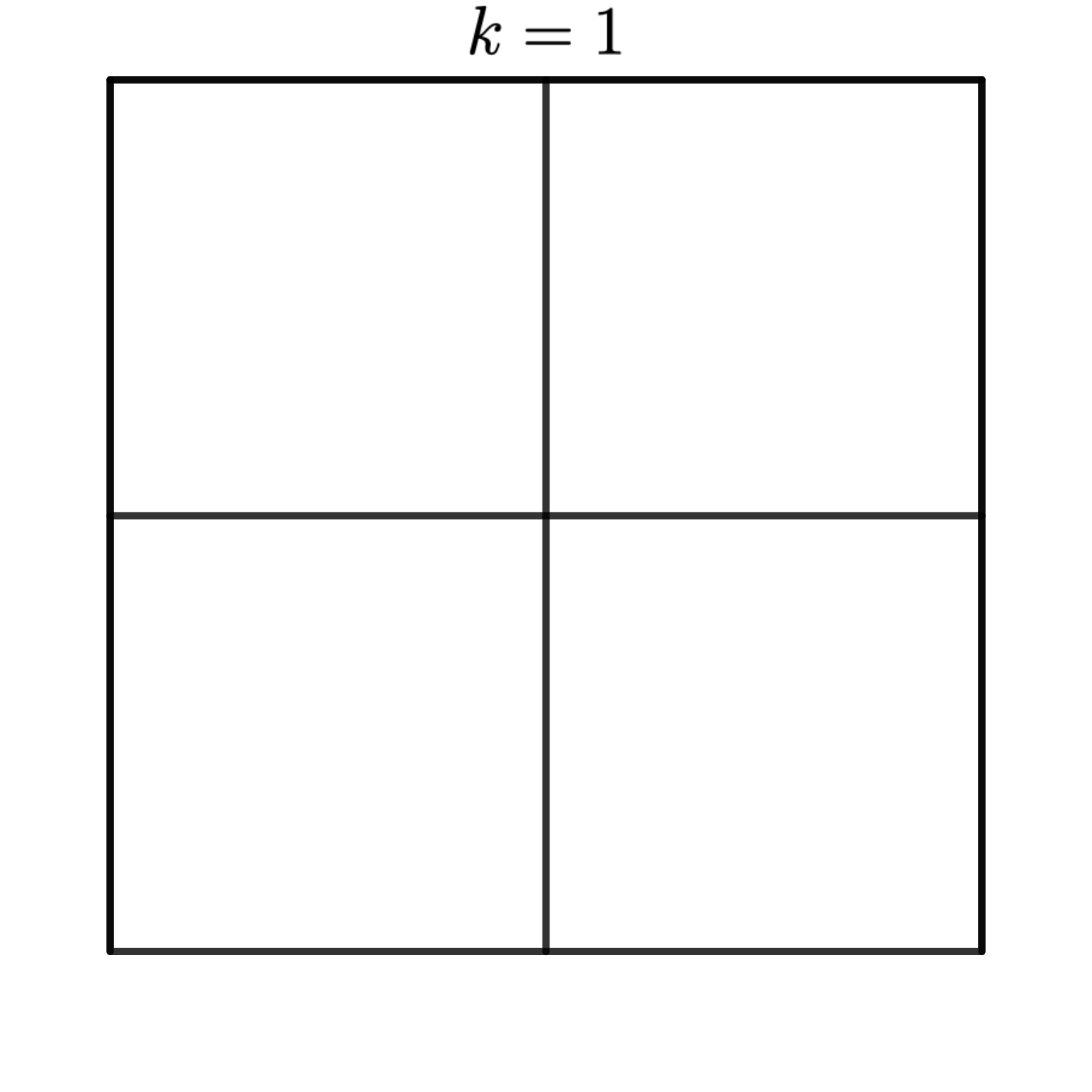
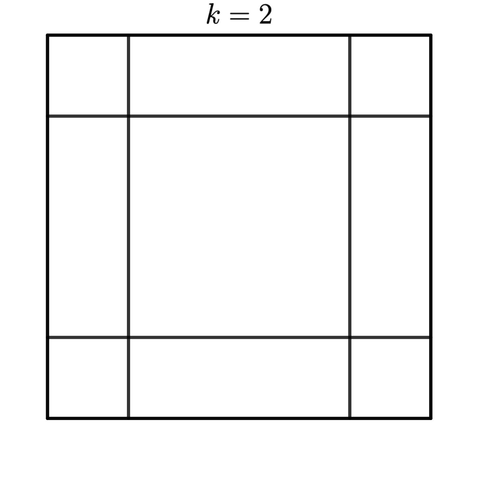
Figure 1: Partitions of a triangular SV for $\mathcal{P}_{k}$ and a rectangular SV for $\mathcal{Q}_{k}$ in 2D with $k=1,2$.

To introduce the OFSV scheme, we first suppose that there exists a partition $\mathcal{T}_{h}$ of $\Omega$ and $\mathcal{T}_{h}$ is shape regular, i.e., there exists a constant $c>0$ such that

$$h\leq ch_{\tau},\ {\rm with}\ h=\displaystyle\max_{\tau\in\mathcal{T}_{h}}h_{\tau},h_{\tau}=\operatorname{diam}\tau,~{}\tau\in\mathcal{T}_{h}.$$

The (discontinuous) finite element space is defined as follows:

$$\mathcal{U}_{h}=\mathcal{U}_{h}^{k}=\{v\in L^{2}(\Omega):\left.v\right|_{\tau}\in\mathcal{P}_{k}\ {\rm or}\ \mathcal{Q}_{k},\tau\in\mathcal{T}_{h}\},$$

where $\mathcal{P}_{k}$ and $\mathcal{Q}_{k}$ denote the finite element space of polynomials with degree not greater than $k$ and the $bi$-$k$ tensor product polynomial space, respectively. In the SV method, a simplex grid element $\tau$, called a spectral volume (SV), is futher divided into non-overlapping sub-elements $\{\tau_{j}^{*}\}_{j}$, named control volumes (CVs). The number of CVs hinges on the cardinality of the polynomials. To illustrate, in 2D case, a SV is segmented into $N$ CVs with $N=(k+1)(k+2)/2$ for $\mathcal{P}_{k}$ elements, and $N=(k+1)^{2}$ for $\mathcal{Q}_{k}$ elements. Figure.1 shows partitions of a triangular SV and a rectangular SV for linear and quadratic elements in 2D.

Denote by ${\mathcal{T}^{*}_{h}}$ the dual partition of ${\mathcal{T}_{h}}$, i.e., ${\mathcal{T}^{*}_{h}}=\{\tau_{j}^{*}:\tau\in{{\mathcal{T}}_{h}}\}.$ The OFSV scheme for equation (1) read as: Seek $\boldsymbol{U}_{h}(\cdot,t)\in\left[\mathcal{U}_{h}^{k}\right]^{m}$ such that for all $\tau_{j}^{*}\in{\mathcal{T}^{*}_{h}}$,

(2) $$\int_{\tau_{j}^{*}}\left(\boldsymbol{U}_{h}\right)_{t}\text{d}\boldsymbol{x}=\int_{\partial\tau_{j}^{*}}\widehat{\boldsymbol{F}}\cdot\boldsymbol{n}\text{d}\Gamma-\sum_{l=0}^{k}\frac{\sigma_{\tau}^{l}}{h_{\tau}}\int_{\tau_{j}^{*}}\left(\boldsymbol{U}_{h}-P_{h}^{l-1}\boldsymbol{U}_{h}\right)\text{d}\boldsymbol{x},$$

where $\widehat{\boldsymbol{F}}=(\widehat{\boldsymbol{F}}_{1},\cdots,\widehat{\boldsymbol{F}}_{d})$, and $\boldsymbol{n}=(n_{1},\cdots,n_{d})$ is the unit outward normal with respect to $\tau_{j}^{*}$. The Gaussian quadrature is used for the integration of numerical fluxes. For the CV interfaces inside the SV, the smooth Euler flux is used. For the SV interfaces, the numerical fluxes are provided by Riemann fluxes to deal with discontinuities, such as Lax-Friedrichs flux and HLLC flux [29]. $P_{h}^{l}$ is the standard $L^{2}$ projection into $[\mathcal{U}_{h}^{l}]^{m},l\geq 0$ with $P_{h}^{-1}=P_{h}^{0}$, and $\sigma_{\tau}^{l}$ are damping coefficients, which are adopted to control spurious oscillations near the discontinuities. The damping coefficients $\sigma_{\tau}^{l}$ are given as follows

(3) $$\sigma_{\tau}^{l}=\frac{2(2l+1)}{(2k-1)}\frac{h^{l}}{l!}\max_{1\leq s\leq m}\sum_{|\boldsymbol{\alpha}|=l}\left(\frac{1}{N_{e}}\sum_{\boldsymbol{v}\in\partial\tau}\left(\left.\llbracket\partial^{\boldsymbol{\alpha}}V_{s}\rrbracket\right|_{\boldsymbol{v}}\right)^{2}\right)^{\frac{1}{2}},$$

where $N_{e}$ is the number of edges of the element $\tau$, $\boldsymbol{v}\in\tau$ are the vertices of $\tau$, $\left.\llbracket w\rrbracket\right|_{\boldsymbol{v}}$ denotes the jump of $w$ on the vertex $\boldsymbol{v}$, $\boldsymbol{\alpha}$ is the multi-index of order $|\boldsymbol{\alpha}|=\alpha_{1}+\cdots+\alpha_{d},$ and $\partial^{\alpha}w$ is defined as

$$\partial^{\boldsymbol{{\boldsymbol{\alpha}}}}\boldsymbol{V}=\frac{\partial^{|\boldsymbol{{\boldsymbol{\alpha}}}|}\boldsymbol{V}}{\partial x_{1}^{\alpha_{1}}\cdots\partial x_{d}^{\alpha_{d}}}=\partial_{x_{1}}^{\alpha_{1}}\cdots\partial_{x_{d}}^{\alpha_{d}}\boldsymbol{V}.$$

Here the variables $\partial_{x}^{l}\boldsymbol{V}=\left(\partial_{x}^{l}V_{1},\ldots,\partial_{x}^{l}V_{m}\right)^{T}$ are given by $\partial_{x}^{l}\boldsymbol{V}=\boldsymbol{R}^{-1}\partial_{x}^{l}\boldsymbol{U}_{h}$, $\boldsymbol{R}$ is the matrix corresponding to right eigenvectors of Jacobian matrix $\partial\boldsymbol{F}/\partial\boldsymbol{U}((\overline{\boldsymbol{U}}_{h})_{i+1/2})$ and $\overline{(\cdot)}_{i+1/2}$ stands for the Roe average of variables at both side of point. The numerical scheme (2) reduces to the standard SV method with $\sigma_{\tau}^{l}=0$.

Remark 2.1.

The introduction of the damping term originates from the OFDG method for hyperbolic conservation laws in [25]. Usually, higher order terms are treated as sources of non-physical spurious oscillation. Therefore, the basic idea is to fix high order term by constructing a serious coefficients, which are small enough in the smooth region to guarantee the high order accuracy and sufficiently large near discontinuities to control spurious oscillations. A natural way to establish the coefficients is adopting the jump of SVs vertexes, but it is not unique. More studies still need to be investigated in the future research.

3 Analysis for constant coefficient hyperbolic problems

This section is dedicated to the analysis of the OFSV method, where the stability, convergence and accuracy are discussed. For simplify and clarity, we focus our attention on the following 1D constant-coefficient linear advection equation

(4) $$\begin{cases}\partial_{t}u+\partial_{x}u=0,&(x,t)\in[a,b]\times(0,T],\\ u(x,0)=u_{0}(x),&x\in(a,b),\end{cases}$$

with the periodic boundary condition $u(a,t)=u(b,t)$ or the inflow boundary condition $u(0,t)=g(t)$. The numerical fluxes are taken as upwind fluxes. We would like to point out that the same argument can be applied to the ${\mathcal{Q}}_{k}$ element for 2D linear scalar equations or systems, with some tedious calculationas.

3.1 OFSV Method as a Petrov Galerkin Method

Let

$${\mathcal{T}}_{h}=\{\tau_{i}:\tau_{i}=(x_{i-\frac{1}{2}},x_{i+\frac{1}{2}}),\ 1\leq i\leq N\}.$$

Assume that the $i$-th SV $\tau_{i}$ is partitioned into $k+1$ CVs with $k$ points $x_{i,j},1\leq j\leq k$, denoted by $\tau_{i,j},j=0,\cdots,k$ with $\tau_{i,j}=(x_{i,j},x_{i,j+1})$. Here $x_{i,0}=x_{i-\frac{1}{2}},x_{i,k+1}=x_{i+\frac{1}{2}}$. Then the dual partition ${\mathcal{T}}_{h}^{*}$ can be expressed by

$${\mathcal{T}}^{*}_{h}=\{\tau_{i,j}:\tau_{i,j}=(x_{i,j},x_{i,j+1}),1\leq i\leq N,0\leq j\leq k\}.$$

Noticing that different choices of the dual partitions (i.e., $x_{i,j}$) leads to different SV scheme, which may have effect on the stability of the numerical scheme. Furthermore, as pointed out in [33], if $x_{i,j}$ are taken as right Radau points, the SV scheme is exactly the same as the standard upwind DG scheme. In this paper, two classes of SV schemes will be analyzed theoretically: 1) $x_{i,j},1\leq j\leq k$ are chosen as the Gauss points; 2) $x_{i,j},1\leq j\leq k$ are taken as the interior right Radau points, (i.e., zeros of $L_{i,k+1}-L_{i,k}$ except the point $x_{i+\frac{1}{2}}$). Here $L_{i,k}$ denotes the Legendre polynomial of degree $k$ in $\tau_{i}$. The corresponding two SV methods are separately referred as the Gauss Legendre spectral volume (OF-LSV) method and the right Radau spectral volume (OF-RRSV) method.

To study the stability of OF-LSV and OF-RRSV, we first rewrite the SV scheme into its equivalent Petrov-Galerkin method. Define the piecewise constant function space as

$$\mathcal{V}_{h}=\left\{w^{*}:w^{*}\mid_{\tau_{i,j}}\in\mathcal{P}_{0},1\leq i\leq N,0\leq j\leq k\right\}.$$

Obviously, any function $w^{*}=w^{*}(x,t)\in\mathcal{V}_{h}$ has the following formulation

$$w^{*}(x,t)=\sum_{i=1}^{N}\sum_{j=0}^{k}w_{i,j}^{*}\chi_{\tau_{i,j}}(x),$$

where $w_{i,j}^{*}=w_{i,j}^{*}(t)$ are coefficients as functions of the variable $t$, and $\chi_{A},A\subset[a,b]$ is the characteristic function valuated $1$ in $A$ and $0$ otherwise. Let

$$\mathcal{H}_{h}=\left\{v:v|_{\tau_{i}}\in H^{1},1\leq i\leq N\right\}.$$

Denote by $a_{h}(\cdot,\cdot)$ the bilinear form defined on $\mathcal{H}_{h}\times\mathcal{V}_{h}$, i.e.,

(5) $$a_{h}\left(v,w^{*}\right)=\sum_{i=1}^{N}a_{h_{i}}\left(v,w^{*}\right),\quad v\in\mathcal{H}_{h},w^{*}\in\mathcal{V}_{h},$$

with

(6) $$a_{h_{i}}\left(v,w^{*}\right):=\sum_{j=0}^{k}w_{i,j}^{*}\big{(}\int_{x_{i,j}}^{x_{i,j+1}}v_{t}dx+v^{-}_{i,j+1}-v^{-}_{i,j}+\displaystyle\sum^{k}_{l=0}\frac{\sigma_{i}^{l}}{h_{i}}\int_{x_{i,j}}^{x_{i,j+1}}(v_{h}-P_{h}^{l-1}v_{h})dx\big{)},$$

with $\sigma_{i}^{l}=\sigma_{{\tau}_{i}}^{l}$ given by (3). Here $v^{-}_{i,j}$ denotes the right limit of $v$ at the point $x_{i,j}$.

Recalling the OFSV scheme in (2), the OFSV method for (4) is to find a $u_{h}\in\mathcal{U}_{h}$ such that

(7) $$a_{h}\left(u_{h},w^{*}\right)=0,\quad\forall w^{*}\in\mathcal{V}_{h}.$$

Conversely, if $u_{h}\in\mathcal{U}_{h}$ satisfies the equation (7), then $u_{h}$ is the solution of (2), by choosing $w^{*}=\chi_{{\tau}_{i,j}}$. In other words, the OFSV method is equivalent to the numerical method (7).

We end with this subsection the discussion about the bilinear form between the OFSV method and the standard SV method. Define the bilinear form $a_{h}^{SV}(\cdot,\cdot)$ of the standard SV method by (see, e.g., [33])

$$a_{h}^{SV}(v,w)=\sum_{i=1}^{N}a_{h_{i}}^{SV}\left(v,w^{*}\right),\ {\rm with}\ a_{h_{i}}^{SV}\left(v,w^{*}\right)=\sum_{j=0}^{k}w_{i,j}^{*}(\int_{x_{i,j}}^{x_{i,j+1}}v_{t}dx+v^{-}_{i,j+1}-v^{-}_{i,j}).$$

In light of (5)-(6), there holds

$$\begin{split}a_{h}\left(v,w^{*}\right)=a_{h}^{SV}(v,w^{*})+\sum^{N}_{i=1}\sum^{k}_{l=0}\frac{\sigma_{i}^{l}}{h_{i}}\left(v-P_{h}^{l-1}v,w^{*}\right).\end{split}$$

3.2 $L^{2}$ stability

We first recall a special transformation the trial space to the test space $\mathcal{F}:\mathcal{U}_{h}\rightarrow\mathcal{V}_{h}$, which is of great importance in our stability analysis. For all $w\in\mathcal{U}_{h}$, let

$$\mathcal{F}w=w^{*}:=\sum_{i=1}^{N}\sum_{j=0}^{k}w_{i,j}^{*}(t)\chi_{{\tau}_{i,j}}(x)\in\mathcal{V}_{h},$$

where the coefficients $w_{i,j}^{*}$ are given as

$$w_{i,0}^{*}=w_{i-\frac{1}{2}}^{+},\quad w_{i,j}^{*}-w_{i,j-1}^{*}=A_{i,j}w_{x}\left(x_{i,j}\right),\ 1\leq j\leq k.$$

Here $A_{i,j}$ denotes the numerical quadrature weights corresponding the points $x_{i,j}$ in $\tau_{i}$. Given any function $v\in{\mathcal{H}}_{h}$, denote by $R_{i}(v)$ the numerical quadrature error between the exact integral and its numerical quadrature $Q_{k}(v)$ in $\tau_{i}$, i.e.,

$$R_{i}(v)=\int_{\tau_{i}}vdx-Q_{k}(v),\ \ {\rm with}\ Q_{k}(v)=\sum_{i=1}^{k+1}A_{i,j}v(x_{i,j}).$$

Define

$$(v,w)_{i}=\int_{\tau_{i}}(vw)dx,\ (v,w)=\sum_{i=1}^{N}(v,w)_{i},\ \ D_{x}^{-1}v=\int_{a}^{x}vdx.$$

It has been proved in [33] that

(8) $$(v,w^{*})_{i}-(v,w)_{i}=R_{i}\left(w_{x}D_{x}^{-1}v\right),\ \ \forall w\in{\mathcal{U}}_{h},w^{*}={\mathcal{F}}w.$$

Due to the identity (8), the bilinear form of the OFSV can be rewritten into

(9) $$a_{h_{i}}\left(v,w^{*}\right)=a_{h_{i}}^{SV}\left(v,w^{*}\right)+\sum^{k}_{l=0}\frac{\sigma_{i}^{l}}{h_{i}}\left(v-P_{h}^{l-1}v,w\right)_{i}+R_{i}\\ \big{(}w_{x}\sum^{k}_{l=0}\frac{\sigma_{i}^{l}}{h_{i}}D^{-1}_{x}(v-P_{h}^{l-1}v)\big{)}.$$

Now we are ready to present the $L^{2}$ stability for both OF-LSV and OF-RRSV method.

Theorem 3.1.

Suppose $u_{h}$ is the solution of (7). Then for both OF-LSV and OF-RRSV,

(10) $$\|u_{h}(\cdot,t)\|_{0}\lesssim\|u_{0}\|_{0},\ \ \forall t>0.$$

Proof 3.2.

Since the $k$-point Gauss numerical quadrature and the $(k+1)$-point right Radau numerical quadrature is separately exact for polynomials of degree $2k-1$ and $2k$, there holds $R_{i}(v)=0,v\in\mathcal{P}_{2k-1}$ for OF-LSV and $R_{i}(v)=0,v\in\mathcal{P}_{2k}$ for OF-RRSV. Then taking $v=w\in\mathcal{U}_{h}$ in (9) and using the orthogonality property of $P_{h}^{l}$ yields

(11) $$a_{h_{i}}\left(v,v^{*}\right)=a_{h_{i}}^{SV}\left(v,v^{*}\right)+\sum^{k}_{l=0}\frac{\sigma_{i}^{l}}{h_{i}}\|v-P_{h}^{l-1}v\|_{0,\tau_{i}}^{2}+R_{i}(v_{x}(\displaystyle\sum^{k}_{l=0}\frac{\sigma_{i}^{l}}{h_{i}}D_{x}^{-1}v)).$$

Noticing that $v_{x}D_{x}^{-1}v|_{\tau_{i}}\in\mathcal{P}_{2k}$ for any $v\in\mathcal{U}_{h}$, we have $R_{i}(v_{x}D_{x}^{-1}v)=0$ for OF-RRSV. As for OF-LSV, by using the error of Gauss-Legendre quadrature, there exists a $\xi_{i}\in\tau_{i}$ such that

(12) $$R_{i}(v_{x}D_{x}^{-1}v)=c_{l}^{k}(\frac{h_{i}}{2})^{2k+1}\partial_{x}^{2k}(v_{x}D_{x}^{-1}v)^{(2k)}(\xi_{i})=c_{l}^{k}(\frac{h_{i}}{2})^{2k}C_{2k}^{k-1}(\partial_{x}^{k}v(\xi_{i}))^{2}\geq 0,$$

where $c_{l}^{k}=\frac{2^{2k+1}(k!)^{4}}{(2k+1)[(2k)!]^{3}}$. Then we conclude from (8) and the inverse inequality that

(13) $$(v,v)\leq(v,v^{*})\lesssim(v,v),\ \ \forall v\in\mathcal{U}_{h}.$$

On the other hand, substituting (12) into (11) and summing up all $i$ from $1$ to $N$ gives

(14) $$a_{h}\left(v,v^{*}\right)\geq a_{h}^{SV}\left(v,v^{*}\right)+\sum_{i=1}^{N}\sum^{k}_{l=0}\frac{\sigma_{i}^{l}}{h_{i}}\|v-P_{h}^{l-1}v\|_{0,{\tau}_{i}}^{2}.$$

Note that (see, e.g., [33])

(15) $$a_{h}^{SV}\left(v,v^{*}\right)=(v_{t},v^{*})+\frac{1}{2}\sum_{i=1}^{N}\left.\llbracket v\rrbracket\right|^{2}_{i+\frac{1}{2}}+\frac{1}{2}(v_{N+\frac{1}{2}}^{-})^{2}-\frac{1}{2}(v_{\frac{1}{2}}^{-})^{2}.$$

By taking $v=u_{h}$ in (14) and using (15) and the $L^{2}$ equivalence (13), then (10) follows.

3.3 Optimal error estimates

We begin with the introduction of a special Lagrange interpolation. For any $v\in\mathcal{H}_{h}$, let $v_{I}\in\mathcal{U}_{h}$ be the Lagrange interpolation of $v$ satisfying the conditions

$$v_{I}\left(x_{i,j}\right)=v\left(x_{i,j}\right),\quad 1\leq i\leq N,1\leq j\leq k+1.$$

The standard approximation theory gives us

$$\left\|v-v_{I}\right\|_{0}\lesssim h^{k+1}\|v\|_{k+1}.$$

The optimal error estimate for both OF-LSV and OF-RRSV methods is presented below.

Theorem 3.3.

Assume $u(\cdot,t)\in H^{k+2}([a,b])$ is the exact solution of (4) and $u_{h}$ is the solution of (7) with the initial solution chosen as $u_{h}(x,0)=(u_{0})_{I}(x)$. Then

(16) $$\left\|(u-u_{h})(\cdot,t)\right\|_{0}\leq Ch^{k+1},$$

where C is a constant, depending on $u$ and its derives up to $(k+2)$-$th$ order.

Proof 3.4.

Let

$$e=u-u_{h},\ \ \xi=u_{I}-u_{h},\eta=u_{I}-u.$$

Since the exact solution $u$ satisfies $a_{h}^{SV}(u,v^{*})=0,\ v\in\mathcal{U}_{h}$, there holds the following orthogonality

$$a_{h}^{SV}(e,v^{*})=\sum_{i=1}^{N}\sum^{k}_{l=0}\frac{\sigma_{i}^{l}}{h_{i}}\left(u_{h}-P_{h}^{l-1}u_{h},v^{*}\right)_{\tau_{i}},\ \ v\in\mathcal{U}_{h}.$$

On the other hand, we choose $v=\xi$ in (14) and use (15) and the above orthogonality, and then obtain

(17) $$(\xi_{t},\xi^{*})+\sum^{N}_{i=1}\sum^{k}_{l=0}\frac{\sigma_{i}^{l}}{h_{i}}\|\xi-P_{h}^{l-1}\xi\|_{0,\tau_{i}}^{2}\leq a_{h}^{SV}(\eta,\xi^{*})+\sum_{i=1}^{N}\sum^{k}_{l=0}\frac{\sigma_{i}^{l}}{h_{i}}\left(u_{I}-P_{h}^{l-1}u_{I},\xi^{*}\right)_{i}.$$

We next estimate the two terms appeared in the right hand side of (17). As for $a_{h}^{SV}(\eta,\xi^{*})$, there holds the conclusion in [33]

(18) $$|a_{h}^{SV}(\eta,\xi^{*})|\lesssim h^{k+1}\|\xi^{*}\|_{0}.$$

Using the Cauchy-Schwarz inequality and the approximation property of $u_{I}$, we get

$$(u_{I}-P_{h}^{l-1}u_{I},\xi^{*})_{i}\leq\|u_{I}-P_{h}^{l-1}u_{I}\|_{0,{\tau}_{i}}\|\xi\|_{0,\tau_{i}}\lesssim h^{\max(1,l)+\frac{1}{2}}\|u_{I}\|_{l,\infty,\tau_{i}}\|\xi\|_{0,\tau_{i}}.$$

Recalling the definition of $\sigma_{i}^{l}$ in (3), there holds

(19) $$\left(\sigma_{i}^{l}\right)^{2} =\frac{4(2l+1)^{2}}{(2k-1)^{2}}\frac{h^{2l}}{(l!)^{2}}\left(\llbracket\partial_{x}^{l}\left(u_{h}-u\right)\rrbracket_{i-\frac{1}{2}}^{2}+\llbracket\partial_{x}^{l}\left(u_{h}-u\right)\rrbracket_{i+\frac{1}{2}}^{2}\right)$$

$$\lesssim h^{2l}\left(\llbracket\partial_{x}^{l}\xi\rrbracket_{i-\frac{1}{2}}^{2}+\llbracket\partial_{x}^{l}\xi\rrbracket_{i+\frac{1}{2}}^{2}\right)+h^{2l}\left(\llbracket\partial_{x}^{l}\eta\rrbracket_{i-\frac{1}{2}}^{2}+\llbracket\partial_{x}^{l}\eta\rrbracket_{i+\frac{1}{2}}^{2}\right).$$

Combining the last two inequalities yields

(20) $$\left|\sum_{i=1}^{N}\sum^{k}_{l=0}\frac{\sigma_{i}^{l}}{h_{i}}\left(u_{I}-P_{h}^{l-1}u_{I}\xi^{*}\right)_{i}\right|$$

$$\lesssim \sum_{i=1}^{N}\sum_{l=0}^{k}h_{i}^{\max\left(l-\frac{1}{2},\frac{1}{2}\right)+l}\left(\llbracket\partial_{x}^{l}\xi\rrbracket_{i-\frac{1}{2}}^{2}+\llbracket\partial_{x}^{l}\eta\rrbracket_{i-\frac{1}{2}}^{2}\right)^{\frac{1}{2}}\|\xi^{*}\|_{0,\tau_{i}}$$

$$\lesssim \|\xi\|_{0}\|\xi^{*}\|_{0}+h^{k+1}\|\xi^{*}\|_{0}.$$

Substituting (18) and (20) into (17) leads to

$$(\xi_{t},\xi^{*})\lesssim\|\xi\|_{0}\|\xi^{*}\|_{0}+h^{k+1}\|\xi^{*}\|_{0}.$$

By using the $L^{2}$ equivalence in (13) and the Gronwall’s inequality, we have

(21) $$\|\xi(\cdot,t)\|_{0}\lesssim\|\xi(\cdot,0)\|_{0}+h^{k+1}.$$

Then (16) follows from the approximation property of $u_{I}$.

3.4 Superconvergence

Following the argument in [33], we adopt the idea of correction function to study the superconvergence property of the OF-LSV and OF-RRSV.

We begin with the construction of the correction function $\omega\in\mathcal{U}_{h}$, which is defined in each element $\tau_{i},1\leq i\leq N$ by

(22) $$\left\{\begin{array}[]{l}\left(\omega,v_{x}\right)_{i}=\left(\partial_{t}\eta,v^{*}\right)_{i}+\displaystyle\sum^{k}_{l=0}\frac{\sigma_{i}^{l}}{h_{i}}\left(u_{I}-P_{h}^{l-1}u_{I},v^{*}\right)_{i},\quad\forall v\in\mathcal{P}_{-}(\tau_{i}),\\ \omega(x_{i+\frac{1}{2}}^{-},t)=0,\end{array}\right.$$

where $\mathcal{P}_{-}$ is the orthogonal complement of $\mathcal{P}^{0}$ in $\mathcal{P}^{k}$, namely, $\mathcal{P}^{k}=\mathcal{P}^{0}\bigoplus\mathcal{P}_{-}$.

Lemma 3.5.

The correction function $\omega$ defined by (22) is uniquely determined. Moreover, if $u\in W^{k+3,\infty}([a,b])$, then

(23) $$\|\partial_{t}^{r}\omega\|_{0}\leq Ch^{k+2},\quad r=0,1.$$

where C is a constant, depending on the exact solution $u$ and its derivative up to $(k+2+r)$-$th$.

Proof 3.6.

Since $\omega|_{\tau_{i}}\in\mathcal{P}^{k}$, we suppose that

$$\omega|_{\tau_{i}}=\sum_{m=0}^{k}c_{i,m}(t)L_{i,m}(x),$$

where $L_{i,m}$ denotes the Legendre polynomial of degree $m$ in $\tau_{i}$. Denoting $\phi_{i,m+1}=\frac{2}{h_{i}}\int_{x_{i-\frac{1}{2}}}^{x}L_{i,m}dx$ and choosing $v=\phi_{i,m+1},m=0,\cdots,k-1$ in (22) yields

$$\frac{2}{h_{i}}\left(\omega,L_{i,m}^{*}\right)_{i}=(\partial_{t}\eta,\phi_{i,m+1}^{*})_{i}+\displaystyle\sum^{k}_{l=0}\frac{\sigma_{i}^{l}}{h_{i}}\left(u_{I}-P_{h}^{l-1}u_{I},\phi_{i,m+1}^{*}\right)_{i}:={\cal H}_{1}+{\cal H}_{2}.$$

As for ${\cal H}_{1}$, it was proved in [33] that

(24) $${\cal H}_{1}\lesssim h^{m^{\prime}}\|u\|_{m^{\prime},\infty,{\tau}_{i}},\quad m^{\prime}=\max(2k+1-m,k+2).$$

To estimate ${\cal H}_{2}$, we have, from (8),

(25) $${\cal H}_{2}=\displaystyle\sum^{k}_{l=0}\frac{\sigma_{i}^{l}}{h_{i}}((u_{I}-P_{h}^{l-1}u_{I},\phi_{i,m+1})_{i}+\frac{2}{h_{i}}R_{i}(L_{i,m}V_{l})),\ {\rm with}\ V_{l}=D_{x}^{-1}(u_{I}-P_{h}^{l-1}u_{I}).$$

Using the fact that right Radau quadrature is exact for $2k$, we have $R_{i}(L_{i,m}V_{l})=0$ for all $0\leq m\leq k-1$ for OF-RRSV. As for OF-LSV, we use the residual of Gauss-Legendre quadrature to derive

$$R_{i}(L_{i,m}V_{l})=R_{i}(L_{i,m}D_{x}^{-1}u_{I})=(\frac{h_{i}}{2})^{2k+1}c_{l}^{k}\partial_{x}^{2k}(L_{i,m}D_{x}^{-1}u_{I})(\xi),\xi\in\tau_{i},$$

which yields, together with the inverse inequality that

$$\frac{2}{h_{i}}|R_{i}(L_{i,m}V_{l})|\lesssim(h_{i})^{2k}\|\partial_{x}^{k-1}L_{i,m}\|_{0,\infty,{\tau}_{i}}\|\partial_{x}^{k}u_{I}\|_{0,\infty,\tau_{i}}\\ \lesssim h_{i}^{k+1}\|u\|_{k,\infty,\tau_{i}}.$$

As a direct consequence of the Cauchy-Schwarz inequality and the approximation property of $P_{h}^{l}$,

$$\left\lvert\left(u_{I}-P_{h}^{l-1}u_{I},\phi_{i,m+1}\right)_{i}\right\rvert\lesssim h_{i}^{\max\{1,l\}+1}\|u\|_{l,\infty,\tau_{i}}.$$

In light of (19) and the estiamte of $\xi$ in (21), we have

$$\left|\sigma_{i}^{l}\right|\lesssim h^{k+1}\|u\|_{k+2,\infty,\tau_{i-1}\cup\tau_{i}\cup\tau_{i+1}}.$$

Substituting the last three inequality into the formulation of ${\cal H}_{2}$ in (25) yields

(26) $$\left\lvert{\cal H}_{2}\right\rvert\lesssim\sum_{l=0}^{k}\left|\sigma_{i}^{l}\right|\cdot h_{i}^{-1}\cdot(h_{i}^{\max\{1,l\}+1}+h_{i}^{k+1})\lesssim h_{i}^{k+2}\|u\|_{k+2,\infty,\tau_{i-1}\cup\tau_{i}\cup\tau_{i+1}}.$$

Combining the estimates of ${\cal H}_{i},1\leq i\leq 2$ in (24) and (26), we have

$$\left\lvert c_{i,m}\right\rvert \lesssim\frac{2}{h_{i}}|\left(\omega,L_{i,m}^{*}\right)_{i}|\lesssim h_{i}^{k+2}\|u\|_{k+2,\infty,\tau_{i-1}\cup\tau_{i}\cup\tau_{i+1}},\ \ m\leq k-1.$$

As for $m=k$, the identity $\omega(x_{i+\frac{1}{2}})^{-}=0$ implies that

$$\left\lvert c_{i,m}\right\rvert=\left\lvert\sum_{n=0}^{k-1}c_{i,n}\right\rvert\lesssim h_{i}^{k+2}\|u\|_{k+2,\infty,\tau_{i-1}\cup\tau_{i}\cup\tau_{i+1}}.$$

Consequently,

$$\left\lVert\omega\right\rVert^{2}_{0}\lesssim\sum_{i=1}^{N}h_{i}\sum_{m=0}^{k}\left\lvert c_{i,m}\right\rvert^{2}\lesssim h^{2(k+2)}\|u\|_{k+2,\infty}.$$

The (23) is valid for $r=0$. Taking time derivative in both sides of (22) and following the same argument, we can prove that (23) also holds true for $r=1$.

Theorem 3.7.

Let $u\in W^{k+3,\infty}(\Omega)$ be the solution of (4), $u_{h}$ be the solution of (7) with the initial solution chosen as $u_{h}(x,0)=\widetilde{(u_{0})}_{I}(x)$. Then for both OF-LSV and OF-RRSV,

(27) $$\|(u_{I}-u_{h})(\cdot,t)\|_{0}\leq Ch^{k+2},$$

where C is a constant, depending on the exact solution $u$ and its $(k+3)$-$th$ derivative.

Proof 3.8.

Denoting

$$\widetilde{u}_{I}=u_{I}-\omega,\quad e=u-u_{h},\quad\xi=u_{h}-\widetilde{u}_{I},\quad\eta=u-\widetilde{u}_{I}.$$

On the one hand, following the same argument as that in (17), we have

(28) $$(\xi_{t},\xi^{*})+\sum^{N}_{i=1}\sum^{k}_{l=0}\frac{\sigma_{i}^{l}}{h_{i}}\|\xi-P_{h}^{l-1}\xi\|_{0}^{2}\leq a_{h}^{SV}(\eta,\xi^{*})+\sum_{i=1}^{N}\sum^{k}_{l=0}\frac{\sigma_{i}^{l}}{h_{i}}\left(\tilde{u}_{I}-P_{h}^{l-1}\tilde{u}_{I},\xi^{*}\right)_{i}.$$

On the other hand, we have for all $v\in\mathcal{P}_{-}$, from (22) that

$$a_{hi}^{SV}(\eta,v^{*})+\sum^{k}_{l=0}\frac{\sigma_{i}^{l}}{h_{i}}\left(\widetilde{u}_{I}-P_{h}^{l-1}\widetilde{u}_{I},v^{*}\right)_{i} = (\partial_{t}\omega,v^{*})_{i}+\sum_{l=0}^{k}\frac{\sigma_{i}^{l}}{h_{i}}\left(\omega-P_{h}^{l-1}\omega,v^{*}\right)_{i}$$

$$\leq\left\lVert\partial_{t}\omega\right\rVert_{0,\tau_{i}}\left\lVert v^{*}\right\rVert_{0,\tau_{i}} + \sum_{l=0}^{k}\frac{\sigma_{i}^{l}}{h_{i}}\left\lVert\omega-P_{h}^{l-1}\omega\right\rVert_{0,\tau_{i}}\left\lVert v^{*}\right\rVert_{0,\tau_{i}}.$$

Summing up all $i$ and using (23) gives

$$a_{h}^{SV}(\eta,v^{*})+\sum_{i=1}^{N}\sum^{k}_{l=0}\frac{\sigma_{i}^{l}}{h_{i}}\left(\widetilde{u}_{I}-P_{h}^{l-1}\widetilde{u}_{I},v^{*}\right)_{i}\lesssim h^{k+2}\left\lVert v^{*}\right\rVert_{0},\ \ \forall v\in\mathcal{P}_{-}.$$

When $v\in\mathcal{P}^{0}$, we easily obtain from the orthogonality of $P^{l}_{h}$ that

$$\sum^{k}_{l=0}\frac{\sigma_{i}^{l}}{h_{i}}\left(\widetilde{u}_{I}-P_{h}^{l-1}\widetilde{u}_{I},v^{*}_{0}\right)_{i}=\sum^{k}_{l=0}\frac{\sigma_{i}^{l}}{h_{i}}\left(\widetilde{u}_{I}-P_{h}^{l-1}\widetilde{u}_{I},v_{0}\right)_{i}=0.$$

Moreover, since it was proved (see Theorem 5.4 in [33]) that

$$|a_{h}^{SV}(\eta,v^{*}_{0})|\lesssim h^{k+2}\left\lVert v_{0}\right\rVert_{0},\ \forall v_{0}\in\mathcal{P}^{0},$$

then

$$a_{h}^{SV}(\eta,v^{*}_{0})+\sum_{i=1}^{N}\sum^{k}_{l=0}\frac{\sigma_{i}^{l}}{h_{i}}\left(\widetilde{u}_{I}-P_{h}^{l-1}\widetilde{u}_{I},v^{*}_{0}\right)_{i}\lesssim h^{k+2}\left\lVert v_{0}^{*}\right\rVert_{0},\ \ v_{0}\in\mathcal{P}^{0}.$$

Note that all the function $v\in\mathcal{U}_{h}$ can be decomposed into $v=v_{0}+v_{1}$ with $v_{0}\in\mathcal{P}^{0}$ and $v_{1}\in\mathcal{P}_{-}$. Consequently,

$$a_{h}^{SV}(\eta,v^{*})+\sum_{i=1}^{N}\sum^{k}_{l=0}\frac{\sigma_{i}^{l}}{h_{i}}\left(\widetilde{u}_{I}-P_{h}^{l-1}\widetilde{u}_{I},v^{*}\right)_{i}\lesssim h^{k+2}\left\lVert v^{*}\right\rVert_{0},\ \ \forall v\in\mathcal{U}_{h}.$$

Substituting the above inequality into (28), we have

$$(\xi_{t},\xi^{*})\lesssim h^{k+2}\|\xi^{*}\|_{0}.$$

Then (27) follows from the the Gronwall’s inequality, the equivalence (13) and the estimate of $\omega$ in (23).

Thanks to the supercloseness result (27) between $u_{I}$ and $u_{h}$, There holds the following superconvergence results for the cell average error and error at downwind points.

Theorem 3.9.

Let $u\in H^{k+3}(\Omega)$ be the solution of (4), $u_{h}$ be the solution of (7) with the initial solution chosen as $u_{h}(x,0)=\widetilde{(u_{0})}_{I}(x)$. Then for both OF-LSV and OF-RRSV,

(29) $$e_{n} :=\left(\frac{1}{N}\sum_{i=1}^{N}\left(u-u_{h}\right)^{2}(x_{i+\frac{1}{2}}^{-},t)\right)^{\frac{1}{2}}\lesssim h^{k+2},$$

$$e_{c} :=\left(\frac{1}{N}\sum_{i=1}^{N}\left(\frac{1}{h_{i}}\int_{\tau_{i}}\left(u-u_{h}\right)dx\right)^{2}\right)^{\frac{1}{2}}\lesssim h^{k+2}.$$

Proof 3.10.

By using the inverse inequality,

$$e_{n}=\left(\frac{1}{N}\sum_{i=1}^{N}\left(u_{I}-u_{h}\right)^{2}(x_{i+\frac{1}{2}}^{-},t)\right)^{\frac{1}{2}}\lesssim\|u_{I}-u_{h}\|_{0}.$$

Then the first inequality of (29) follows from (27). Similarly, since (see, [33])

$$\left(\frac{1}{N}\sum_{i=1}^{N}\left(\frac{1}{h_{i}}\int_{\tau_{i}}\left(u-u_{I}\right)dx\right)^{2}\right)^{\frac{1}{2}}\lesssim h^{k+2},$$

then

$$e_{c}=\left(\frac{1}{N}\sum_{i=1}^{N}\left(\frac{1}{h_{i}}\int_{\tau_{i}}\left(u-u_{I}+u_{I}-u_{h}\right)dx\right)^{2}\right)^{\frac{1}{2}}\lesssim h^{k+2}+\|u_{I}-u_{h}\|_{0},$$

which yields (together with (27)) the second inequality of (29).

4 Numerical experiments

In this section, the numerical tests will be presented to validate the accuracy, robustness of current scheme. The accuracy tests are provided for the linear advection equation and Euler solutions. The ninth-order strong stability preserving (SSP) Runge-Kutta method is applied as temporal discretization aimed at avoiding the interference of temporal discretization on the convergence rates. For the flows with discontinuities, a few benchmark cases for Euler solutions are provided. The specific heat ratio takes $\gamma=1.4$, and the classic fourth order Runge-Kutta method is used for temporal discretization. The CFL condition is

$$\Delta t=\frac{CFL}{(\alpha+a_{0})}\Delta x,~{}\alpha=\max_{i,s}\left|\left(\lambda_{s}\right)_{i+1/2}^{\pm}\right|,~{}a_{0}={\displaystyle\max_{i\in\mathcal{Z}_{N}}}\sum_{l=0}^{k}\sigma_{i}^{l},$$

where $\Delta t$ and $\Delta x$ are time step and cell size, $\left(\lambda_{s}\right)_{i+1/2}^{\pm}$ are real eigenvalues of the Jacobian matrix $\partial\boldsymbol{F}/\partial\boldsymbol{U}$ at $x_{i+1/2}^{\pm}$ and $\sigma_{i}^{l}$ is the damping coefficient defined in (3). This reveals that the time step is severely limited by the coefficient $a_{0}$. In the computation, the CFL number takes $2.4$. $\mathcal{Q}_{k}$ with $k=2$ and $3$ are used for the accuracy tests, and $\mathcal{Q}_{k}$ with $k=2$ is only used for the cases with discontinuities. The mesh with uniform SVs are used for 1D cases, and the uniform rectangular meshes are used for 2D cases. Since the numberical solution of OF-LSV and OF-RRSV are resemblance, only the results of OF-LSV are presented.

4.1 Accuracy tests

In order to verify the order of optimal convergence and superconvergence of current scheme, the one-dimensional and two-dimensional cases are provided. In our numerical experiments, the $L^{2}$ error $\|e_{0}\|_{0}$, the cell average error $e_{c}$ and the average error at downwind points $e_{n}$ will be tested.

The first case is given for one-dimensional linear scalar equation (4), and the initial condition is set as follows

$$u(x)=1+0.2\sin(\pi x).$$

The computation domain $\Omega=[0,2]$ and the periodic boundary condition is adopted at both ends. The analytic solution is

$$u(x,t)=1+0.2\sin(\pi(x-t)).$$

The uniform mesh with $N$ SVs are used. The errors and the order of convergence for $\|e_{0}\|_{0}$, $e_{c}$ and $e_{n}$ are presented in Table 2 at $t=2$. The obtained order in Table 2 are consistent with the analysis in Theorem 3.3 and Theorem 3.9, i.e., $(k+1)$-$th$ optimal convergence order for $\|e_{0}\|_{0}$, both $(k+2)$-$th$ convergence order for both $e_{c}$ and $e_{n}$. In order to investigate the effect of damping term on accuracy, this example is also tested by the classical SV method with $k=2$ and $3$. The errors and the order of convergence are listed in Table 2. The expected orders for SV method in [33] are verified, i.e., the optimal convergence rate $(k+1)$ for the $L^{2}$ error $\|e\|_{0}$, and the convergence rate $(2k)$ for both the cell average error $e_{c}$ and the error at downwind point $e_{n}$. With the mesh refinement, the $L^{2}$ error $\|e_{0}\|_{0}$ of OFSV method and SV method get closer, which means the damping term becomes smaller for the smooth analytic solution. However, the damping term does affect on the superconvergence accuracy.

Table 1: One-dimensional accuracy test: errors and convergence orders of $\|e_{0}\|_{0}$, $e_{c}$, $e_{n}$ for OFSV scheme.

$k$	Mesh	$\|e_{0}\|_{0}$	order	$e_{c}$	order	$e_{n}$	order
	$8$	4.9119E-03		2.2847E-03		2.4315E-03
	$16$	3.5267E-04	3.8000	1.5955E-04	3.8399	1.6600E-04	3.8727
2	$32$	2.4316E-05	3.8583	9.2332E-06	4.1110	9.3982E-06	4.1426
	$64$	2.1921E-06	3.4715	5.3050E-07	4.1214	5.3672E-07	4.1301
	$128$	2.4509E-07	3.1609	3.1495E-08	4.0742	3.1815E-08	4.0764
	$8$	2.0132E-04		1.3213E-04		1.3945E-04
	$16$	6.2608E-06	5.0070	4.0326E-06	5.0341	4.1981E-06	5.0539
3	$32$	2.3475E-07	4.7371	1.3517E-07	4.8988	1.3820E-07	4.9249
	$64$	1.0447E-08	4.4900	4.5274E-09	4.9000	4.5788E-09	4.9156
	$128$	5.5435E-10	4.2361	1.4816E-10	4.9334	1.4915E-10	4.9401

Table 2: One-dimensional accuracy test: errors and convergence orders of $\|e_{0}\|_{0}$, $e_{c}$, $e_{n}$ for SV scheme.

$k$	Mesh	$\|e_{0}\|_{0}$	order	$e_{c}$	order	$e_{n}$	order
	$8$	1.1168E-03		2.8677E-04		3.0598E-04
	$16$	1.2537E-04	3.1551	1.9091E-05	3.9089	1.9951E-05	3.9389
2	$32$	1.5151E-05	3.0488	1.2196E-06	3.9647	1.2674E-06	3.9765
	$64$	1.8767E-06	3.0130	7.6902E-08	3.9872	7.9807E-08	3.9892
	$128$	2.3405E-07	3.0033	4.8272E-09	3.9938	5.0093E-09	3.9938
	$8$	5.0192E-05		1.2012E-06		5.4416E-06
	$16$	2.9697E-06	4.0791	2.7583E-08	5.4446	3.0592E-08	7.4747
3	$32$	1.8558E-07	4.0002	4.3641E-10	5.9820	4.7041E-10	6.0231
	$64$	1.1599E-08	4.0000	6.8475E-12	5.9939	7.3725E-12	5.9956
	$128$	7.2493E-10	4.0000	2.9283E-13	4.5474	2.9877E-13	4.6351

Table 3: Two-dimensional accuracy test: errors and convergence orders of $\|e_{0}\|_{0}$, $e_{c}$, $e_{n}$ for OFSV scheme.

$k$	Mesh	$\|e_{0}\|_{0}$	order	$e_{c}$	order	$e_{n}$	order
	$8^{2}$	1.8533E-02		9.7494E-03		9.6293E-03
	$16^{2}$	1.2227E-03	3.9219	5.8527E-04	3.9020	6.2540E-04	3.9446
2	$32^{2}$	7.4101E-05	4.0445	3.5010E-05	4.0633	3.6142E-05	4.1130
	$64^{2}$	4.9616E-06	3.9006	2.0624E-06	4.0854	2.0998E-06	4.1054
	$128^{2}$	4.2071E-07	3.5617	1.2461E-07	4.0488	1.2623E-07	4.0560
	$8^{2}$	1.4675E-03		6.7864E-04		7.5641E-04
	$16^{2}$	3.4150E-05	5.4254	1.6197E-05	5.3889	1.7362E-05	5.4452
3	$32^{2}$	1.0958E-06	4.9619	5.2147E-07	4.9570	5.4169E-07	5.0023
	$64^{2}$	3.9061E-08	4.8100	1.7557E-08	4.8925	1.7918E-08	4.9180
	$128^{2}$	1.5517E-09	4.6539	5.7939E-10	4.9214	5.5602E-10	4.9343

Table 4: Two-dimensional accuracy test: errors and convergence orders of $\|e_{0}\|_{0}$, $e_{c}$, $e_{n}$ for SV scheme.

$k$	Mesh	$\|e_{0}\|_{0}$	order	$e_{c}$	order	$e_{n}$	order
	$8^{2}$	1.7926E-03		5.5948E-04		6.1273E-04
	$16^{2}$	1.8552E-04	3.2724	3.8014E-05	3.8795	4.0014E-05	3.9367
2	$32^{2}$	2.1701E-05	3.0957	2.4428E-06	3.9599	2.5469E-06	3.9737
	$64^{2}$	2.6629E-06	3.0267	1.5457E-07	3.9822	1.6100E-07	3.9836
	$128^{2}$	3.3127E-07	3.0069	9.7551E-09	3.9859	1.0190E-08	3.9818
	$8^{2}$	7.1124E-05		2.3412E-06		1.0883E-06
	$16^{2}$	4.2004E-06	4.0817	5.4813E-08	5.4166	6.1185E-08	7.4747
3	$32^{2}$	2.6246E-07	4.0004	8.7141E-10	5.9750	9.4081E-10	6.0231
	$64^{2}$	1.6403E-08	4.0000	1.3685E-11	5.9927	1.4738E-11	5.9963
	$128^{2}$	1.0252E-09	4.0000	3.5470E-13	5.2698	3.6942E-13	5.3182

The second case for accuracy is the advection of density perturbation for two-dimensional Euler equations, and the initial conditions are given follows

$$\rho_{0}(x,y)=1+0.2\sin(\pi(x+y)),~{}p_{0}(x,y)=1,~{}U_{0}(x,y)=1,~{}V_{0}(x,y)=1.$$

The computational domain is $[0,2]\times[0,2]$ and the periodic boundary conditions are adopted in both directions. The analytic solutions are

$$\rho(x,y,t)=1+0.2\sin(\pi((x+y)-2t)),~{}p(x,y,t)=1,~{}U(x,y,t)=1,~{}V(x,y,t)=1.$$

The uniform mesh with $N^{2}$ SVs are used in the computation. The errors and convergence orders, including $\|e_{0}\|$,$e_{c}$,$e_{n}$, are presented in Table.4 at $t=2$. The expected order of accuracy are obtained. As reference, this case is also tested by the classical SV method. The errors and convergence orders are presented in Table.4. The numerical results indicate the damping term would not pollute the optimal order of accuracy and reduce the order of superconvergence for the Euler equations as well.

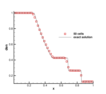
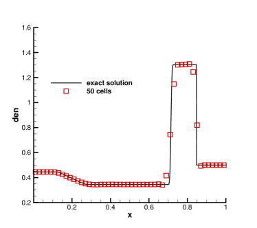
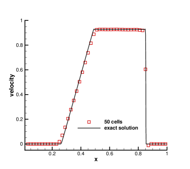
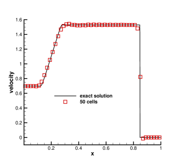
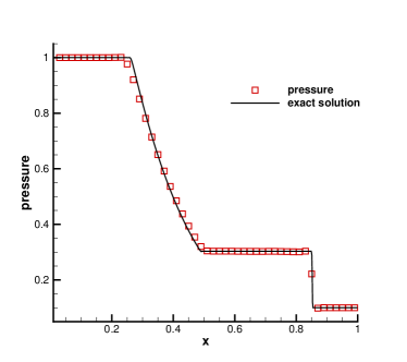
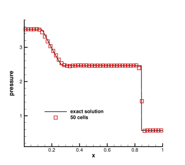
Figure 2: One-dimensional Riemann problem: the density, velocity and pressure distributions for Sod problem (left) at $t=0.2$, and Lax problem (right) at $t=0.14$.

4.2 One-dimensional Riemann problems

In this case, two Riemann problems of one-dimensional Euler equations are tested. The first test is Sod problem and the initial conditions are given as follows

$$(\rho,U,p)=\begin{cases}(1,0,1),&0\leq x<0.5,\\ (0.125,0,0.1),&0.5\leq x\leq 1.\end{cases}$$

The second one is Lax problem and the initial conditions are given as follows

$$(\rho,U,p)=\begin{cases}(0.445,0.698,3.528),&0\leq x<0.5,\\ (0.5,0,0.571),&0.5\leq x\leq 1.\end{cases}$$

For these two tests, the computational domain is $[0,1]$ with 50 uniform SVs and non-reflecting boundary condition is adopted on both ends. The cell average of density, velocity, and pressure distributions for the third-order OFSV method and the exact solutions are presented in Figure.2 for Sod problem at $t=0.2$ and for Lax problem at $t=0.14$. The numerical results agree well with the exact solutions and the spurious oscillations are effectively restrained.

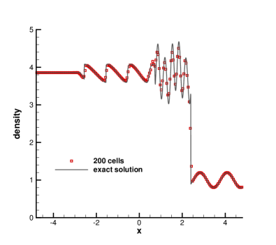
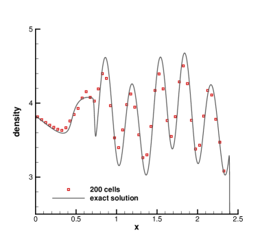
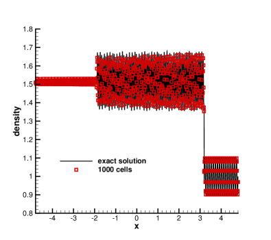
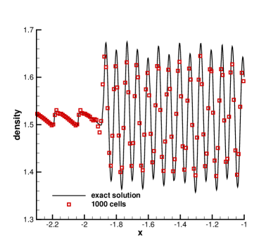
Figure 3: Shu-Osher problem: the density distribution and local enlargement at $t=2$.

Figure 4: Titarev-Toro problem: the density distribution and local enlargement at $t=5$.

4.3 Shock-acoustic interactions

For the one-dimensional case, another test case is the Shu-Osher shock acoustic interaction [11], describing the interaction between a right moving Mach $3$ shock interacting with a sine wave in density. This is a typical example to show the advantage of a high order scheme because both shocks and complex smooth region structures coexist. The computational domain is taken to be $[-5,5]$, and the initial conditions are given as

$$(\rho,U,p)=\begin{cases}(3.857134,2.629369,10.33333),&-5\leq x\leq-4,\\ (1+0.2\sin(5x),0,1),&-4<x<5.\end{cases}$$

Uniform mesh with $200$ SVs is used. The cell average of density distribution and local enlargement are presented in Figure. 4 at $t=2$, where the reference solution is given by the fifth order finite volume WENO method with $1000$ cells. The numerical solutions also agree well with the reference solution, which shows that the current scheme controls the spurious oscillation effectively.

As an extension of Shu-Osher problem, Titarev-Toro shock wave interaction problem [35] is also tested, which simulates a severely oscillatory wave interacting with shock. The computational domain is also taken to be $[-5,5]$, and the initial conditions for this case are given as follows

$$(\rho,U,p)=\begin{cases}(1.515695,0.523346,1.805),&-5<x\leq-4.5,\\ (1+0.1\sin(20\pi x),0,1).&-4.5<x<5.\end{cases}$$

Uniform mesh with $1000$ SVs is used. The density distribution and local enlargement at $t=5$ are presented in Figure.4, where the reference solution is given by the fifth-order finite volume WENO method with $4000$ cells. The numerical result shows that OFSV method does have the ability of high-order numerical scheme to capture the extremely high frequency waves and eliminate the spurious oscillations.

4.4 Two-dimensional Riemann problems

In this case, two examples of two-dimensional Riemann problems [36] are presented, including the interactions of shocks and the interaction of contacts with rarefaction waves. The computational domain is both $[0,1]\times[0,1]$, and the non-reflecting boundary conditions are used in all ends. The initial conditions for the first case are

$$(\rho,U,V,p)=\begin{cases}(1.5,0,0,1.5),&x>0.5,y>0.5,\\ (0.5323,1.206,0,0.3),&x<0.5,y>0.5,\\ (0.138,1.206,1.206,0.029),&x<0.5,y<0.5,\\ (0.5323,0,1.206,0.3),&x>0.5,y<0.5.\end{cases}$$

A complicated pattern is evolved by the interaction between the four initial shock waves. The density distributions and the local enlargements are showed at $t=0.3$ in Figure.5 with $400\times 400$ and $800\times 800$ uniform SVs. The numerical results show that the small scale flow structures are well captured by the current scheme.

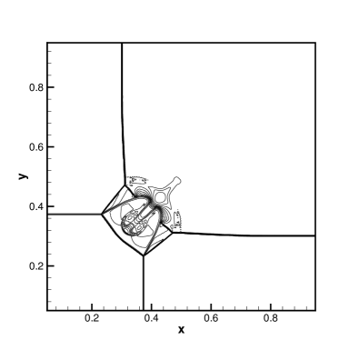
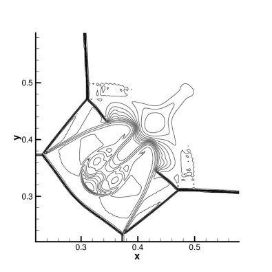
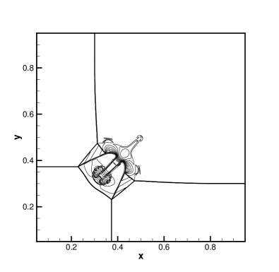
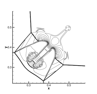
Figure 5: Two-dimensional Riemann problem: the density distributions and local enlargements for the first case at $t=0.3$ with $400\times 400$ (top) and $800\times 800$ (bottom) uniform SVs.

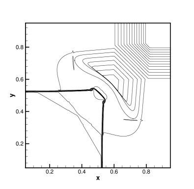
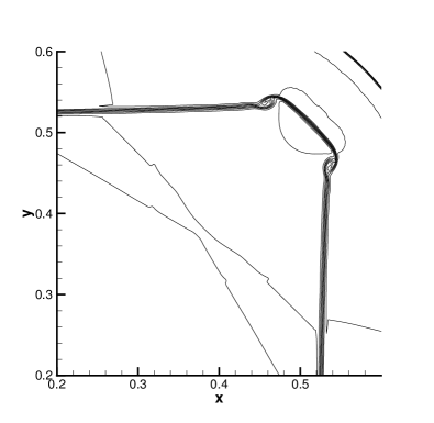
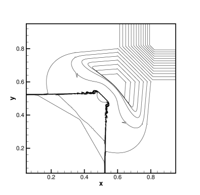
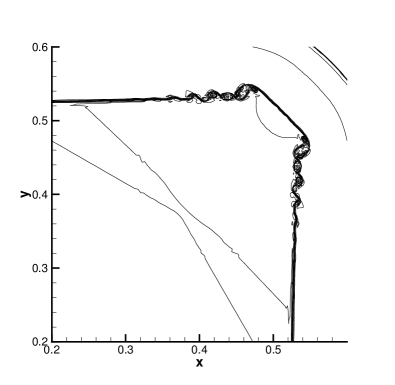
Figure 6: Two-dimensional Riemann problem: the density distributions and local enlargements for the second case at $t=0.25$ with $300\times 300$ (top) and $600\times 600$ (bottom) uniform SVs.

The second case is to simulate the interaction between the interaction of two contacts with two rarefaction waves, and the initial conditions are given as

$$(\rho,U,V,p)=\begin{cases}(1,0.1,0.1,1),&x>0.5,y>0.5,\\ (0.5197,-0.6259,0.1,0.4),&x<0.5,y>0.5,\\ (0.8,0.1,0.1,0.4),&x<0.5,y<0.5,\\ (0.5197,0.1,-0.6259,0.4),&x>0.5,y<0.5.\end{cases}$$

The density distributions and the local enlargements at $t=0.25$ are given in Figure.6 with $300\times 300$ and $600\times 600$ uniform SVs. The results validate the good behavior of the current method by which the roll-up is well captured.

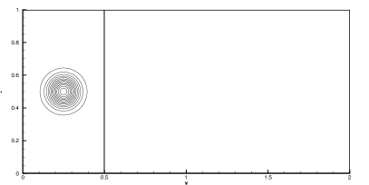
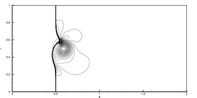
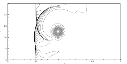
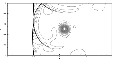
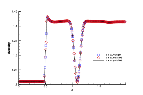
Figure 7: Shock vortex interaction: the pressure distributions at $t=0,0.3,0.6$ and $0.8$ with $400\times 200$ cells.

Figure 8: Shock vortex interaction: the density distributions at $t=0.8$ along the horizontal symmetric line $y=0.5$ with mesh size $\Delta x=\Delta y=1/50,1/100,1/200$.

4.5 Shock-vortex interaction

The interaction between a stationary shock and a vortex for the inviscid flow [13] is presented. The computational domain is taken to be $[0,2]\times[0,1]$. A stationary Mach $1.1$ shock is positioned at $x=0.5$ and vertical to the $x$-axis. The left upstream state is $(\rho,U,V,p)=\left(Ma^{2},\sqrt{\gamma},0,1\right)$, where $Ma$ is the Mach number. A slight vortex perturbation centered at $\left(x_{c},y_{c}\right)=(0.25,0.5)$ is added to the mean flow with the velocity $(U,V)$, temperature $T=p/\rho$, and entropy $S=\ln\left(p/\rho^{\gamma}\right)$, expressed as

$$(\delta U,\delta V)=\kappa\eta e^{\mu\left(1-\eta^{2}\right)}(\sin\theta,-\cos\theta),$$

and

$$\delta T=-\frac{(\gamma-1)\kappa^{2}}{4\mu\gamma}e^{2\mu\left(1-\eta^{2}\right)},\delta S=0,$$

where $\eta=r/r_{c}$, $r=\sqrt{\left(x-x_{c}\right)^{2}+\left(y-y_{c}\right)^{2}}$, $\kappa$ implies the strength of the vortex, $\mu$ controls the decay rate of the vortex, and $r_{c}$ is the critical radius of the vortex with maximum strength. In the computation, these parameters are taken as $\kappa=0.3,\mu=0.204$, and $r_{c}=0.05$. The reflecting boundary conditions are used on the top and bottom boundaries. The inflow and outflow boundary conditions are used for the left and right boundaries. This case is tested by the uniform SVs with $\Delta x=\Delta y=1/50,1/100$ and $1/200$. The pressure distributions with $\Delta x=\Delta y=1/200$ at $t=0,0.3,0.6$ and $0.8$ are shown in Figure.8. By $t=0.8$, one branch of the shock bifurcations has reflected on the upper boundary and this reflection is well captured. The detailed density distributions along the center horizontal line with mesh size $\Delta x=\Delta y=1/50,1/100$ and $1/200$ at $t=0.8$ presented in Figure.8 are convergent. Satisfactory results are obtained and the accuracy of the scheme is well demonstrated.

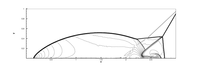
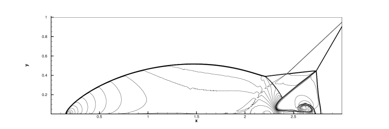
Figure 9: Double Mach reflections: the density distributions at $t=0.2$ with $800\times 200$ (top) and $1600\times 400$ (bottom) uniform SVs.

4.6 Double Mach reflection

This problem was first proposed by Woodward and Colella [37] for the inviscid flow. The computational domain is $[0,4]\times[0,1]$ and a reflecting solid wall lies along the bottom of the computational domain starting from $x=1/6$. Initially a right-moving Mach 10 shock makes a $60^{\circ}$ angle with the reflecting wall starting at $(x,y)=(1/6,0)$ towards the top of the computational domain. The initial pre-shock and post-shock conditions are

$$(\rho,U,V,p)=\begin{cases}\left(8,4.125\sqrt{3},-4.125,116.5\right),&x<\frac{1}{6}+\frac{1}{\sqrt{3}}y,\\ \left(1.4,0,0,1\right),&x>\frac{1}{6}+\frac{1}{\sqrt{3}}y.\end{cases}$$

The inflow and outflow boundary conditions are adopted for the left and right boundaries, respectively. The reflecting boundary condition is used at the solid wall, and the exact post-shock condition is imposed for the rest of the bottom boundary. At the top boundary, the flow variables are set to describe the exact motion of the Mach 10 shock. The density distributions and their local enlargement with $800\times 200$ and $1600\times 400$ uniform SVs at $t=0.2$ are presented in Figure.9 and Figure.10, respectively. The flow structure under the triple Mach stem can be resolved clearly. However, the shear layer seems to be smeared by the damping term, and more delicate design of damping term still needs to be investigated in the future.

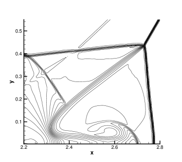
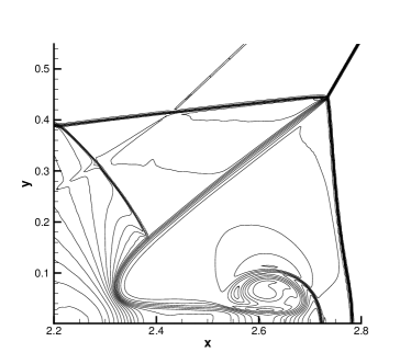
Figure 10: Double Mach reflections: the local enlargement of density distributions at $t=0.2$ with $800\times 200$ (left) and $1600\times 400$ (right) uniform SVs.

5 Conclusion

In this paper, an oscillation-free spectral volume method is proposed for the systems of hyperbolic conservation laws. To suppress the oscillations near discontinuities, a damping term is introduced to the standard spectral volume method. A mathematical proof is provided to show that the proposed OFSV is stable and has optimal convergence rate and some excepted superconvergence properties when applied to linear scalar equations. Numerical experiments are presented to demonstrate the accuracy and capabilities of resolving discontinuities for the current scheme. The excepted order of accuracy of the current SV scheme is obtained, and the oscillations can be well controlled even for the problem with strong discontinuities.

References

- [1] W. H. Reed, T. R. Hill, Triangular mesh methods for the neutron transport equation, Los Alamos scientific laboratory report, LA-UR-73-479, (1973).
- [2] B. Cockburn, C.-W Shu, TVB Runge-Kutta local projection discontinuous Galerkin finite element method for conservation laws. II. General framework, Math. Comp., 52.186 (1989), pp. 411-435.
- [3] B. Cockburn, C.-W. Shu, The Runge-Kutta discontinuous Galerkin method for conservation laws V: multidimensional systems, J. Comput. Phys., 141.2 (1998), pp. 199-224.
- [4] Y. Sun and Z. Wang, Evaluation of discontinuous Galerkin and spectral volume methods for scalar and system conservation laws unstructured grids. Int. J .Numer. Meth. Fluids, 45 (2004) 819-838.
- [5] Z. J. Wang, Y. Liu, Spectral (finite) volume method for conservation laws on unstructured grids III: One dimensional systems and partition optimization, J. Sci. Comput., 20.1 (2004), pp. 137-157.
- [6] Y. Liu, M. Vinokur, Z. J. Wang, Spectral (finite) volume method for conservation laws on unstructured grids V: Extension to three-dimensional systems, J. Comput. Phys., 212.2 (2006), pp. 454-472.
- [7] Y. Z. Sun, Z. J. Wang, Y. Liu, Spectral (finite) volume method for conservation laws on unstructured grids VI: Extension to viscous flow, J. Comput. Phys., 215.1 (2006), pp. 41-58.
- [8] Y. Liu, M. Vinokur, Z. J. Wang, Spectral difference method for unstructured grids I: Basic formulation, J. Comput. Phys., 216.2 (2006), pp. 780-801.
- [9] H. T. Huynh, Z. J. Wang, P. E. Vincent, High-order methods for computational fluid dynamics: A brief review of compact differential formulations on unstructured grids, Comput. & Fluids, 98 (2014), pp. 209-220.
- [10] A. Harten, B. Engquist, S. Osher, S. R. Chakravarthy, Uniformly high order accurate essentially non-oscillatory schemes, III, J. Comput. Phys., 71 (1987), pp. 231-303.
- [11] C.-W. Shu, S. Osher, Efficient implementation of essentially non-oscillatory shock-capturing schemes, J. Comput. Phys., 77.2 (1988), pp. 439-471.
- [12] X. D. Liu, S. Osher, T. Chan, Weighted essentially non-oscillatory schemes, J. Comput. Phys., 115.1 (1994), pp. 200-212.
- [13] G. S. Jiang, C.-W. Shu, Efficient implementation of weighted ENO schemes, J. Comput. Phys., 126.1 (1996), pp. 202-228.
- [14] R. Borges, M. Carmona, B. Costaand, W.S. Don, An improved weighted essentially non-oscillatory scheme for hyperbolic conservation laws, J. Comput. Phys., 227.6 (2008), pp. 3191-3211.
- [15] J. X. Qiu, C.-W. Shu, Hermite WENO schemes and their application as limiters for Runge-Kutta discontinuous Galerkin method: one-dimensional case, J. Comput. Phys., 193.1 (2004), pp. 115-135.
- [16] J. X. Qiu, C.-W. Shu, Hermite WENO schemes and their application as limiters for Runge-Kutta discontinuous Galerkin method II: Two dimensional case, Comput. & Fluids, 34.6 (2005), pp. 642-663.
- [17] H. Luo, J. D. Baum, R. Löhner, A Hermite WENO-based limiter for discontinuous Galerkin method on unstructured grids, J. Comput. Phys., 225.1 (2007), pp. 686-713.
- [18] B. Cockburn, S. Y. Lin, C.-W. Shu, TVB Runge-Kutta local projection discontinuous Galerkin finite element method for conservation laws III: one-dimensional systems, J. Comput. Phys., 84.1 (1989), pp. 90-113.
- [19] B. Cockburn, S. Hou, C.-W. Shu, The Runge-Kutta local projection discontinuous Galerkin finite element method for conservation laws. IV. The multidimensional case, Math. Comp., 54.190 (1990), pp. 545-581.
- [20] B. van Leer, Toward the ultimate conservative difference scheme. V. A second order sequel to Godunov method, J. Comp. Phys., 32 (1979) 101-136.
- [21] C. Hu, C.-W. Shu, Weighted essentially non-oscillatory schemes on triangular meshes, J. Comput. Phys., 150 (1999), pp. 97–127.
- [22] J. X. Qiu, C.-W. Shu, Runge–Kutta discontinuous Galerkin method using WENO limiters, SIAM J. Sci. Comput., 26 (2005), pp. 907-929.
- [23] J. Zhu, J. Qiu, Runge-Kutta discontinuous Galerkin method using WENO-type limiters: three-dimensional unstructured meshes, Commun. Comput. Phys., 11.3 (2012), pp. 985-1005.
- [24] A. Hiltebrand, S. Mishra, Entropy stable shock capturing space-time discontinuous Galerkin schemes for systems of conservation laws, Numer. Math., 126.1 (2014), pp. 103-151.
- [25] J. F. Lu, Y. Liu, C.-W. Shu, An oscillation-free discontinuous Galerkin method for scalar hyperbolic conservation laws, SIAM J. Numer. Anal., 59.3 (2021), pp. 1299-1324.
- [26] Y. Liu, J. F. Lu, C.-W. Shu, An Essentially Oscillation-Free Discontinuous Galerkin Method for Hyperbolic Systems, SIAM J. Sci. Comput., 44.1 (2022), pp. 230-259.
- [27] Y. Liu, J. F. Lu, Q. Tao and Y. Xia, An Oscillation-free Discontinuous Galerkin Method for Shallow Water Equations, J. Sci. Comput., 92.3 (2022), pp. 1-24.
- [28] S. K. Godunov, A difference scheme for numerical computation of discontinuous solution of hyperbolic equation, Math. Sbornik., 47 (1959), pp. 271-306.
- [29] E. Toro, Riemann Solvers and Numerical Methods for Fluid Dynamics, Springer, (1997).
- [30] B. J. Choi, M. Iskandarani, J. Levin, D. B. Haidvogel, A spectral finite-volume method for the shallow water equations, Mon. Weather Rev., 132.7 (2004), pp. 1777-1791.
- [31] Y. Z. Sun, Z. J. Wang, High-order spectral volume method for the Navier-Stokes equations on unstructured grids, 34th AIAA Fluid Dynamics Conference and Exhibit, 2004.
- [32] Y. Z. Sun, Z. J. Wang, Y. Liu, High-order multidomain spectral difference method for the Navier-Stokes equations, 44th AIAA Aerospace Sciences Meeting and Exhibit, 2006.
- [33] W. X. Cao, Q. S. Zou, Analysis of Spectral Volume Methods for 1D Linear Scalar Hyperbolic Equations, J. Sci. Comput., 90.1 (2022), pp. 1-29.
- [34] M. Zhang, C.-W. Shu, An analysis of and a comparison between the discontinuous Galerkin and the spectral finite volume methods, Comput. & Fluids, 34.4-5 (2005), pp. 581-592.
- [35] V. A. Titarev, E. F. Toro, Finite-volume WENO schemes for three-dimensional conservation laws, J. Comput. Phys., 201.1 (2004), pp. 238-260.
- [36] P. D. Lax, X.D. Liu, Solution of two-dimensional riemann problems of gas dynamics by positive schemes, SIAM J. Sci. Comput. 19 (1998), pp. 319-340.
- [37] P. Woodward and P. Colella, The numerical simulation of two-dimensional fluid flow with strong shocks, J. Comput. Phys., 54.1 (1984), pp. 115-173.