Nuclear quadrupole resonance spectroscopy with a femtotesla diamond magnetometer

Abstract

Sensitive Radio-Frequency (RF) magnetometers that can detect oscillating magnetic fields at the femtotesla level are needed for demanding applications such as Nuclear Quadrupole Resonance (NQR) spectroscopy. RF magnetometers based on Nitrogen-Vacancy (NV) centers in diamond have been predicted to offer femtotesla sensitivity, but published experiments have largely been limited to the picotesla level. Here, we demonstrate a femtotesla RF magnetometer based on an NV-doped diamond membrane inserted between two ferrite flux concentrators. The device operates in bias magnetic fields of $2\mbox{-}10~{}{\rm\upmu T}$ and provides a ${\sim}300$-fold amplitude enhancement within the diamond for RF magnetic fields in the $0.07\mbox{-}3.6~{}{\rm MHz}$ range. The magnetometer’s sensitivity is ${\sim}70~{}{\rm fT\,s^{1/2}}$ at $0.35~{}{\rm MHz}$, and the noise floor decreases to below $2~{}{\rm fT}$ after $1~{}{\rm hour}$ of acquisition. We used this sensor to detect the $3.6~{}{\rm MHz}$ NQR signal of ${}^{14}{\rm N}$ in sodium nitrite powder at room temperature. NQR signals are amplified by a resonant RF coil wrapped around the sample, allowing for higher signal-to-noise ratio detection. The diamond RF magnetometer’s recovery time after a strong RF pulse is ${\sim}35~{}{\rm\upmu s}$, limited by the coil ring-down time. The sodium-nitrite NQR frequency shifts linearly with temperature as $\mbox{-}1.00\,{\pm}\,0.02~{}{\rm kHz/K}$, the magnetization dephasing time is $T_{2}^{\ast}=887\pm 51~{}{\rm\upmu s}$, and a spin-lock spin-echo pulse sequence extends the signal lifetime to $332\,{\pm}\,23~{}{\rm ms}$, all consistent with coil-based NQR studies. Our results expand the sensitivity frontier of diamond magnetometers to the femtotesla range, with potential applications in security, medical imaging, and materials science.

Introduction

Magnetometers based on negatively-charged Nitrogen-Vacancy (NV) centers in diamond are promising room-temperature sensors for detecting magnetic phenomena across a wide range of frequencies Barry et al. (2020). Over the last decade, various sensing protocols and fabrication methods have been developed to improve the sensitivity of diamond magnetometers in the sub-$10\mbox{-}{\rm kHz}$ Barry et al. (2016); Fescenko et al. (2020); Eisenach et al. (2021); Zhang et al. (2021), Radio-Frequency (RF) Masuyama et al. (2018); Glenn et al. (2018); Smits et al. (2019), and microwave (MW) Wang et al. (2022); Alsid et al. (2022) frequency ranges. However, the best reported sensitivities, ${\sim}1~{}{\rm pT\,s^{1/2}}$ Fescenko et al. (2020), still trail the achievable levels in magnetometers based on alkali-metal vapor Savukov et al. (2005); Ledbetter et al. (2007); Griffith et al. (2010); Wasilewski et al. (2010); Dhombridge et al. (2022); Chalupczak et al. (2012); Keder et al. (2014) and superconducting quantum interference devices Clarke (1980); Schmelz et al. (2016); Storm et al. (2017).

Recently, magnetic flux concentrators have been used to improve the performance of diamond magnetometers Fescenko et al. (2020); Zhang et al. (2021); Li et al. (2021); Xie et al. (2022), and a sub-picotesla sensitivity has been realized for low frequencies (${\lesssim 1\,{\rm kHz}}$) by inserting an NV-doped diamond membrane between two ferrite cones Fescenko et al. (2020). We hypothesized that the same approach can be used for improving the sensitivity in the RF range (kHz-MHz) if the flux concentrator’s magnetic properties do not degrade at such frequencies. In fact, better sensitivity may be expected in the RF range, since the diamond RF magnetometer can operate in a pulsed regime where the NV spin coherence time is significantly longer Taylor et al. (2008).

A diamond RF magnetometer with femtotesla sensitivity may find immediate application as a non-inductive detector for Nuclear Quadrupole Resonance (NQR) spectroscopy Connor et al. (1990); Augustine et al. (1998); Lee et al. (2006). NQR spectroscopy is a solid-state analysis technique that provides a unique chemical fingerprint based on the coupling of nuclear quadrupole moments to their local electric field gradients Das and Hahn (1958); Zax et al. (1985). NQR spectroscopy is used to identify powder substances in ambient conditions for security Garroway et al. (2001); Kim et al. (2014); Malone et al. (2020) and pharmaceutical Balchin et al. (2005); Lužnik et al. (2013); Kyriakidou et al. (2015) applications and to study the temperature-dependent properties of single-crystal materials Lyfar et al. (1976); Sharma et al. (1986); Horiuchi et al. (1990); Huebner et al. (1999); Lang et al. (2010). These applications typically require the ability to detect kHz-MHz frequencies, at low bias magnetic fields $\lesssim 1~{}{\rm mT}$, with femtotesla sensitivity Malone et al. (2016). Previously, NV centers were used to detect NQR signals arising from nanoscale statistical polarization in single-crystal boron-nitride layers in direct contact with the diamond Lovchinsky et al. (2017); Henshaw et al. (2022). However, using NV centers to remotely detect powders remains an open challenge due to the need for high sensitivity Shin et al. (2014).

In this paper, we demonstrate a frequency-tunable diamond RF magnetometer with a sensitivity of ${\sim}70~{}{\rm fT\,s^{1/2}}$ at $0.35~{}{\rm MHz}$, using ferrite flux concentrators Fescenko et al. (2020) and a multi-pulse synchronized readout scheme Glenn et al. (2018); Smits et al. (2019). The sensitivity remains within a factor of three of this value for the $0.07{-}3.6~{}{\rm MHz}$ frequency range. We used the magnetometer to detect the $3.6~{}{\rm MHz}$ NQR signal of ${}^{14}{\rm N}$ in sodium nitrite powder samples Oja et al. (1967); Petersen and Bray (1976). Our work expands the sensitivity frontier of diamond magnetometry to the femtotesla range and introduces a new method for remote detection of solid-state magnetic resonance.

Experimental design

A schematic of the diamond RF magnetometer is shown in Fig. 1(a). The apparatus is similar to one previously used for low-frequency magnetometry Fescenko et al. (2020), with modifications (Appendix A) made for RF magnetometry and NQR spectroscopy. For example, the mu-metal shield is replaced by an aluminum shield to suppress RF interference. A thermal-insulation housing with thermoelectric temperature control is added around the shield to improve thermal stability. Calibrated RF test fields with a magnitude $B_{\rm test}$ and frequency $f_{\rm test}$ are applied along the magnetometer sensing axis ($z$-axis) using a pair of low-inductance rectangular wire loops.

A permanent magnet is used to compensate the ambient magnetic field and apply a weak bias field, $B_{0}=2\mbox{-}10~{}{\rm\upmu T}$, approximately along the $z$-axis. The flux concentrators enhance the $z$-component of the magnetic field in the gap between the cone tips. An NV-doped diamond membrane is positioned in the gap with its (100) crystal faces normal to the $z$-axis. This geometry results in two NV spin transition frequencies $f_{\pm}\approx D\,\pm\,\epsilon\gamma_{\rm nv}B_{0}/\sqrt{3}$, where $D=2.87~{}{\rm GHz}$ is the NV zero field splitting, $\epsilon$ is the flux-concentrator enhancement factor ($\epsilon\approx 300$ for DC fields) Fescenko et al. (2020), $\gamma_{\rm nv}=28~{}{\rm GHz/T}$ is the NV gyromagnetic ratio, and the factor of $\sqrt{3}$ comes from the $55\degree$ angle of each NV axis with respect to the $z$-axis.

Figure 1(b) shows the XY8-$N$ synchronized readout pulse sequence used for diamond RF magnetometry Smits et al. (2019). This pulse sequence contains a series of short MW pulses ($10\mbox{-}70~{}{\rm ns}$), of alternating phase, that are tuned to one of the $f_{\pm}$ resonances in the $2.7\mbox{-}3.0~{}{\rm GHz}$ range. Each XY8-$N$ sequence is followed by a $12\mbox{-}{\rm\upmu s}$ laser pulse ($0.2~{}{\rm W}$, $532~{}{\rm nm}$), generated with an acousto-optic modulator, for optical readout and spin polarization of the NV centers. The sequence is repeated continuously, and the resulting time trace of NV fluorescence readouts is approximately proportional to an aliased version of the applied RF field sampled at the time of the first $\pi/2$ pulse of each XY8-$N$ sequence (1). For a magnetic field oscillating with frequency $f$, the NV fluorescence signal oscillates with an alias frequency $f_{\rm alias}=f-f_{\rm ref}$. The reference frequency, $f_{\rm ref}$, depends on the sampling rate $1/\tau_{\rm sample}$, which is adjusted by varying a sub-${\rm\upmu s}$ dead time after each XY8-$N$ sequence Smits et al. (2019).

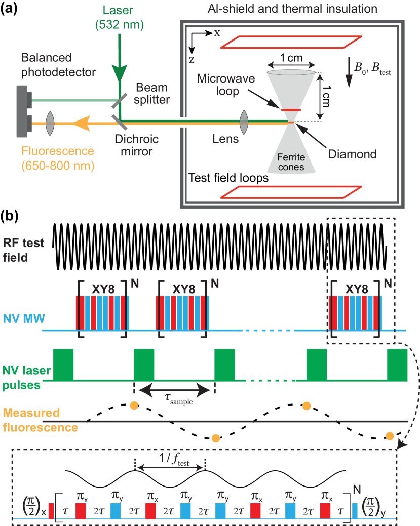
Figure 1: Experimental setup and RF detection scheme. (a) Schematic of the experimental setup for detecting RF test fields. A permanent magnet (not shown) outside of the Al-shield was used to apply weak bias magnetic fields along the $z$-axis, $B_{\rm 0}\,{=}\,2\mbox{-}10~{}{\rm\upmu T}$. Additional details of the setup can be found in Appendix A and Ref. Fescenko et al. (2020). (b) Diamond RF magnetometry is performed with a continuous series of repeated XY8-$N$ pulse sequences on the NV electron spins Smits et al. (2019). Each XY8-$N$ sequence begins and ends with a resonant microwave (MW) $\pi/2$ pulse. Between the $\pi/2$ pulses, $8N$ resonant $\pi$-pulses, spaced by $2\tau=1/(2f_{\rm test}$), are applied with alternating phase. Following each XY8-$N$ sequence, a $12\mbox{-}{\rm\upmu s}$ laser pulse ($0.2~{}{\rm W}$, $532~{}{\rm nm}$) is applied for optical readout and repolarization of the NV centers. The resulting time trace of NV fluorescence readouts is proportional to an aliased version of the RF test field.

A theoretical bound on the diamond RF magnetometer sensitivity is set by photoelectron shot noise as:

$$\eta_{\rm psn}~{}{\approx}~{}\frac{\sqrt{3}\,\xi}{\epsilon\,\sqrt{\delta}}\frac{1}{4\,\gamma_{\rm nv}\,C\sqrt{n_{\rm nv}\,V_{\rm sen}\,\phi\,\tau_{\rm tot}}}.$$ (1)

In the first term of Eq. 1, the $\sqrt{3}$ factor comes from the $55\degree$ angle of each NV axis with respect to the $z$-axis, $\xi\,{=}\,1.6$ accounts for additional photoelectron noise arising from the balanced detection and normalization procedure (1), and $\delta\,{=}\,\tau_{\rm tot}/\tau_{\rm sample}\,{\approx}\,0.75$ is a duty cycle, where $\tau_{\rm tot}$ is the NV phase accumulation time and $\tau_{\rm sample}$ is the sequence repetition time. In the second term, $C$ is the XY8-$N$ fluorescence contrast (1), $n_{\rm nv}$ is the NV concentration, $V_{\rm sen}$ is the illuminated NV sensor volume, and $\phi$ is the probability of detecting a photoelectron per NV center for a single readout.

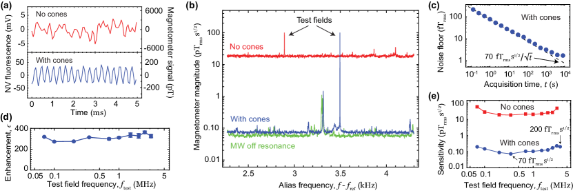
Figure 2: Femtotesla diamond RF magnetometry. (a) Real-time NV fluorescence signal with (blue) and without (red) ferrite cones in the magnetometer assembly. In each case, an XY8-4 synchronized readout sequence was used, and a $0.35~{}{\rm MHz}$ test field with $100~{}{\rm pT_{rms}}$ amplitude was applied. The NV fluorescence photodetector voltage is converted to magnetic field units using the procedure described in 1. For the same applied field amplitude, the photodetector voltage signal with cones is ${\sim}220$ times larger than that without cones, due primarily to the flux concentrator enhancement (and, to a lesser extent, differences in the photon collection efficiency). A digital $4.5~{}{\rm kHz}$ low-pass filter was applied to the data without cones for better visualization. (b) Fourier transform spectra of the NV signals with and without the cones. No digital filtering was applied. The noise floor reaches ${\sim}70~{}{\rm fT\,s^{1/2}}$ with the cones and ${\sim}18~{}{\rm pT\,s^{1/2}}$ without them. A reference spectrum (green), obtained by detuning the MW frequency $200~{}{\rm MHz}$ off the NV resonance, shows an effective noise floor of ${\sim}60~{}{\rm fT\,s^{1/2}}$. (c) Noise floor with the cones present as a function of acquisition time, $t$. (d) Ferrite cones enhancement factor versus the test field frequency (2). (e) Diamond RF magnetometer sensitivity as a function of test field frequency with (blue circles) and without (red squares) the ferrite cones (Appendix D). For all data in this figure, except for the “MW off resonance” spectrum in (b), the MW frequency was tuned to one of the NV $f_{\pm}$ resonances.

The natural-isotopic-abundance single-crystal diamond membrane used in this work contained an initial nitrogen concentration of ${\sim}20~{}{\rm ppm}$. The diamond was doped with NV centers by electron irradiation and annealing (Appendix A), resulting in an NV concentration of $n_{\rm nv}\approx 3~{}{\rm ppm}$ and a transverse NV spin coherence time of ${\sim}50~{}{\rm\upmu s}$ for an XY8-4 sequence. The diamond was subsequently cut and polished into a (100)-oriented membrane with dimensions ${\sim}300\times 300\times 35~{}{\rm\upmu m^{3}}$. The NV sensor volume is defined by the area of the illuminating laser beam and the length of its path in the diamond as $V_{\rm sen}\approx 2\times 10^{5}~{}{\rm\upmu m^{3}}$. The peak detected photoelectron current was typically ${\sim}0.17~{}{\rm mA}$ over a $2~{}{\rm\upmu s}$ readout window, which indicates the detection efficiency of our setup is $\phi\approx 0.02$. We found the best sensitivity of our setup to occur for XY8-4 sequences at $f_{\rm test}=0.35~{}{\rm MHz}$, where $\tau_{\rm tot}=44~{}{\rm\upmu s}$ and $C\approx 0.01$. With these values, and assuming the flux-concentrator enhancement factor $\epsilon\approx 300$ is the same as for DC fields, Eq. (1) predicts a photoelectron-shot-noise-limited sensitivity $\eta_{\rm psn}\approx 30~{}{\rm fT\,s^{1/2}}$.

Magnetometer characterization

We measured the magnetometer’s sensitivity as a function of test field frequency and acquisition time. First, we applied a test field with frequency $f_{\rm test}=0.35~{}{\rm MHz}$ and magnitude $B_{\rm test}=100~{}{\rm pT_{rms}}$ (1) and recorded the magnetometer signal under an XY8-4 synchronized readout sequence for 100 s with and without the ferrite cones. Figure 2(a) shows the real-time NV fluorescence signal for a segment of each time trace. While the magnetometer signal without ferrite cones is dominated by noise, a clear oscillation at frequency $f_{\rm test}-f_{\rm ref}=3.5~{}{\rm kHz}$ is observed with the cones present.

To determine the magnetometer sensitivity, each $100~{}{\rm s}$ NV time trace is divided into one hundred $1~{}{\rm s}$ segments, a spectrum is obtained for each segment by taking the absolute value of the Fourier transform, and the 100 spectra are averaged together. Figure 2(b) shows the resulting magnetic spectra for the recordings with and without the ferrite cones. The magnetic field sensitivity, defined here as the average noise floor for $1\mbox{-}{\rm s}$ acquisition time in a few-hundred-Hz band near the signal frequency (Appendix D), is ${\sim}70~{}{\rm fT_{rms}\,s^{1/2}}$ with the cones and ${\sim}18~{}{\rm pT_{rms}\,s^{1/2}}$ without them. A reference spectrum (with ferrite cones) was obtained by detuning the MW frequency $200~{}{\rm MHz}$ off the NV resonance, revealing an effective noise floor of ${\sim}60~{}{\rm fT_{rms}\,s^{1/2}}$. While the ${\sim}70~{}{\rm fT_{rms}\,s^{1/2}}$ measured noise floor with ferrite cones is ${\sim}2$ times greater than the photoelectron-shot-noise estimate (2), the experimental sensitivity represents a ${\gtrsim}10$-fold improvement over previous diamond magnetometry studies Fescenko et al. (2020) and a ${\gtrsim}100$-fold improvement over previous diamond studies in the RF range Masuyama et al. (2018); Glenn et al. (2018); Smits et al. (2019).

To characterize temporal stability, we continuously recorded the ferrite-cones diamond RF magnetometer signal for several hours. Figure 2(c) shows the magnetic noise floor as a function of averaging time, $t$. We find that the noise floor scales with the expected ${\sim}70~{}{\rm fT\,s^{1/2}}/{\sqrt{t}}$ behavior out to $t\gtrsim 10^{3}~{}{\rm s}$. The noise floor decreases to below $2~{}{\rm fT}$ after 1 hour of acquisition, before leveling off.

We used ferrite cones made of a manganese-zinc material (MN60) that is usually considered more suitable for low-frequency (${\lesssim}\,1~{}{\rm MHz}$) applications National Magnetics Group-Inc. (2019), and it was initially unclear whether large enhancement factors would be possible at higher frequency Bolton (2016). To probe the frequency dependence, we recorded the diamond RF magnetometer signal for different values of $f_{\rm test}$. The enhancement factor provided by the ferrite cones is defined as $\epsilon=B_{\rm gap}/B_{\rm test}$, where $B_{\rm gap}$ is the magnetic field amplitude within the diamond when the cones are present. For each value of $f_{\rm test}$, we calibrated $B_{\rm test}$ by recording the NV signal amplitude (without cones) as a function of the current amplitude applied to the test field loops. We repeated the process with the cones present to calibrate $B_{\rm gap}$. At each frequency, $\epsilon$ was estimated from the ratio of the response curves (2). The results are shown in Fig. 2(d). Surprisingly, we find the enhancement factor is nearly constant ($\epsilon\approx 300$) in the $0.07{-}3.12~{}{\rm MHz}$ frequency range.

We also determined the magnetic sensitivity as a function of frequency, using the process described for Fig. 2(a,b). Figure 2(e) shows the sensitivity as a function of $f_{\rm test}$. For each frequency, the duration and spacing of the MW pulses and the length of the XY8-$N$ sequence were modified to maximize sensitivity (see Table A2 in Appendix D). With the cones, the best sensitivity is ${\sim}70~{}{\rm fT\,s^{1/2}}$ at $f_{\rm test}=0.35~{}{\rm MHz}$, and the sensitivity remains within a factor of 3 of this value throughout the range $0.07\mbox{-}3.62~{}{\rm MHz}$. A diamond with a lower nitrogen concentration, and thus longer coherence time, can be used to extend the frequency range down to ${\sim}1~{}{\rm kHz}$ Barry et al. (2020). A stronger MW field, combined with a higher-NV-concentration diamond (to limit the number of MW pulses without sacrificing sensitivity), could extend the frequency up to ${\gtrsim}10~{}{\rm MHz}$, as long as the ferrite’s permeability and relative loss factor do not degrade Fescenko et al. (2020).

Figure 3: NQR setup. (a) Schematic of the setup used for NQR spectroscopy. A bias field $B_{0}\approx 10~{}{\rm\upmu T}$ is applied along the $z$-axis. An NaNO₂ sample is housed in a plastic cylinder container and placed $d\approx 4~{}{\rm mm}$ above the ferrite-cones diamond RF magnetometer. A resonant RF coil is wrapped around the sample container. The $3.6~{}{\rm MHz}$ NQR transition of ${}^{14}{\rm N}$ nuclei in ${\rm NaNO}_{\rm 2}$ is excited by applying RF pulses along the $z$-axis. The resulting oscillating nuclear magnetic field is also along the $z$-axis and is simultaneously detected by the ferrite-cones diamond RF magnetometer and the resonant RF coil (see 5). (b) Energy levels and nuclear spin transitions of ${}^{14}{\rm N}$ in ${\rm NaNO}_{\rm 2}$ at room temperature and low ($\lesssim 1~{}{\rm mT}$) magnetic field. (c) Initial magnetic field amplitude within the diamond, $B_{\rm gap,i}$ (left axis), and equivalent magnetic field, $B_{\rm equiv,i}=B_{\rm gap,i}/300$ (right axis), as a function of sample volume. expt. – experiment. (d) Pulse sequence used for NV NQR detection (1). After an RF excitation pulse, an XY8-20 synchronized readout pulse sequence is used to detect an aliased version of the nuclear AC magnetic field. The entire sequence is repeated every $T_{\rm rep}=0.5~{}{\rm s}$.

NQR spectroscopy of NaNO₂ powder

IV.1 Experimental design and theoretical estimates

Having demonstrated femtotesla sensitivity in the RF range, we next used our ferrite-cones diamond RF magnetometer as a detector in NQR spectroscopy. The sample we selected to study is sodium nitrite (NaNO₂) powder (2), a well-studied standard for ¹⁴N NQR spectroscopy Fisher et al. (1999); Hiblot et al. (2008). Figure 3(a) shows a schematic of the NQR detection setup. A resonant RF coil is wrapped around a NaNO₂ powder sample, and the sample is placed ${\sim}4~{}{\rm mm}$ above the ferrite-cones diamond RF magnetometer. Two coil assemblies are used: one for a $4\mbox{-}{\rm gram}$ sample and the other for a $21\mbox{-}{\rm gram}$ sample. A capacitor tuning circuit and pi-network are used for conventional inductive detection (5).

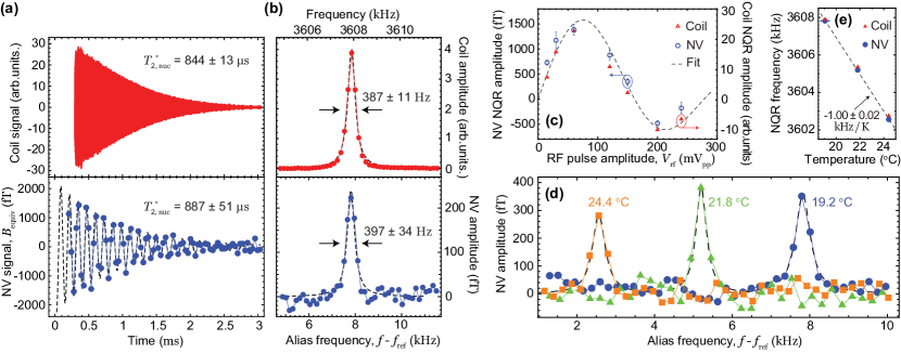
Figure 4: NQR spectroscopy of $\bm{{}^{14}{\rm N}}$ in NaNO₂. (a) Room-temperature time-domain NQR signal of ${}^{14}{\rm N}$ in a 21-gram NaNO₂ powder sample acquired by the resonant RF coil (top) and diamond RF magnetometer (bottom). A $50\mbox{-}{\rm\upmu s}$ RF pulse at $3605~{}{\rm kHz}$ was used to excite the sample via the resonant RF coil with loaded quality factor $Q\,{\approx}\,23$ (see 5). The sequence was repeated every $500~{}{\rm ms}$, and the signal was averaged over 86000 repetitions. A digital bandpass filter is applied for better visualization: $3.58\mbox{-}3.63~{}{\rm MHz}$ for the coil signal and $4.6\mbox{-}11.7~{}{\rm kHz}$ for the NV signal. A decaying sinusoidal function fit to the NV signal reveals an initial amplitude $B_{\rm equiv,i}=2300\pm 115~{}{\rm fT}$ and nuclear dephasing time $T_{\rm 2,\,nuc}^{\ast}=887\pm 51~{}{\rm\upmu s}$. (b) Imaginary part of the Fourier transform of the time-domain NQR signals shown in (a), along with Lorentzian fits. (c) NQR signal amplitude as a function of RF pulse amplitude, $V_{\rm rf}$ (measured in volts, prior to amplification), applied at $3607.5~{}{\rm kHz}$ for $300~{}{\rm\upmu s}$. For each RF pulse amplitude, the imaginary part of the Fourier transform of the first $810~{}{\rm\upmu s}$ of the signals is calculated, such that the NQR resonance is contained in a single frequency point. The value of that point is taken as the NQR amplitude, and the error bars are the standard deviation of points within a $5~{}{\rm kHz}$ band near resonance. The dashed black line is a fit to a function $J_{\rm 3/2}({\alpha})/{\sqrt{\alpha}}$ with the first peak occurring at the nutation angle $\alpha=119^{\degree}$ Vega (1974). (d) NV NQR spectra (imaginary part of Fourier transform) obtained for three different ambient temperatures, along with Lorentzian fits. RF pulses were applied at $3605~{}{\rm kHz}$ for $50\mbox{-}{\rm\upmu s}$. (e) NQR resonance frequency as a function of ambient temperature, along with linear fit.

The nuclear quadrupole Hamiltonian is given by Suits (2006):

$$H_{\rm Q}\,{=}\,f_{\rm Q}\,[I_{\rm z^{{}^{\prime}}}^{2}+\frac{\eta}{3}(I_{\rm x^{{}^{\prime}}}^{2}-I_{\rm y^{{}^{\prime}}}^{2})],$$ (2)

where $f_{\rm Q}$ is the quadrupole coupling frequency, $\eta$ is the asymmetry parameter, and $\{I_{\rm x^{{}^{\prime}}},I_{\rm y^{{}^{\prime}}},I_{\rm z^{{}^{\prime}}}\}$ are the spin components along the principle axes of a given crystallite. As depicted in Fig. 3(b), at low magnetic field ($B_{0}\lesssim 1~{}{\rm mT}$), the ${}^{14}{\rm N}$ nucleus in NaNO₂ ($I{=}1$, $f_{\rm Q}{=}4.1~{}{\rm MHz}$, $\eta{=}0.38$) has three non-degenerate energy levels, $\{E_{\rm z^{{}^{\prime}}},E_{\rm x^{{}^{\prime}}},E_{\rm y^{{}^{\prime}}}\}$, and magnetic-dipole transitions are allowed between each level Oja et al. (1967). We used our sensor to detect the $E_{\rm z^{{}^{\prime}}}\leftrightarrow E_{\rm x^{{}^{\prime}}}$ transition at $f_{\rm nqr}=f_{\rm Q}(1-\eta/3)=3.6~{}{\rm MHz}$. For powder samples, where many crystallites are randomly oriented, application of a resonant RF pulse along the $z$-axis produces a net oscillating magnetization (frequency $f_{\rm nqr}$) along the $z$-axis Bloom et al. (1955), see Appendix F. Thus, to maximize the NQR signal, the RF coil axis was aligned with the magnetometer detection axis, Fig. 3(a).

We carried out simulations to estimate the oscillating magnetic field amplitude produced by cylindrical NaNO₂ samples following an optimal RF excitation pulse on the $3.6~{}{\rm MHz}$ transition. The initial amplitude of the oscillating sample magnetization was estimated to be $M_{0}=3.3~{}{\rm\upmu A/m}$ along the $z$-axis (see Appendix F). A finite-element model was used to make a preliminary estimate of the resulting initial magnetic field amplitude in the diamond when the ferrite cones were present, $B_{\rm gap,i}$. For this and all subsequent NQR measurements, $B_{\rm gap}$ is converted to an equivalent magnetic field $B_{\rm equiv}=B_{\rm gap}/\epsilon$, using $\epsilon=300$ (see 2), to compare with the case of uniform magnetic fields.

For a given sample volume $V_{s}$, we swept the cylinder aspect ratio to estimate the maximum possible nuclear field amplitude (Appendix G). Figure 3(c) shows the maximum simulated $B_{\rm equiv,i}$ as a function of sample volume. The estimated $B_{\rm equiv,i}$ values are at the few-hundred femtotesla level for the $V_{s}=1\mbox{-}10^{3}~{}{\rm cm^{3}}$ range. Figure 3(c) also shows experimentally-measured NQR signals from two sample masses (these measurements are described below). The experimental values are $3\mbox{-}6$ times larger than the simulated estimates, despite several optimistic assumptions such as perfect powder packing, optimal RF excitation pulse, and ideal sample aspect ratio. As discussed below, this difference is due to signal amplification from the resonant RF coil used in the experiment.

Figure 3(d) shows the pulse sequence used for NQR spectroscopy. RF excitation pulses (typically $50\mbox{-}200~{}{\rm\upmu s}$) are applied to the resonant RF coil, and the oscillating nuclear magnetic field is detected by the diamond RF magnetometer using a series of repeated XY8-20 pulse sequences with $f_{\rm ref}=3600.07~{}{\rm kHz}$. After a duration $T_{\rm rep}\approx 0.5~{}{\rm s}$, chosen to be comparable to the ¹⁴N thermal relaxation time, $T_{\rm 1,\,nuc}\approx 0.3~{}{\rm s}$ Petersen and Bray (1976), the entire sequence is repeated. To compare to conventional NQR detection, the same coil is also used to detect the signal inductively after it is passed through a pi-network and amplified by a low-noise pre-amplifier, (see Fig. 3(a), 5).

IV.2 Experimental results with a single RF pulse

Figure 4(a) shows the NQR signals of the 21-gram NaNO₂ powder sample detected by the resonant RF coil and ferrite-cones diamond RF magnetometer. The signals are fit with exponentially-decaying sinusoidal functions, and the fitted $1/e$ decay times are $T_{\rm 2,\,nuc}^{\ast}\,{=}\,844\pm 13~{}{\rm\upmu s}$ for the coil signal and $T_{\rm 2,\,nuc}^{\ast}\,{=}\,887\pm 51~{}{\rm\upmu s}$ for the NV signal. These values are in good agreement with each other and consistent with literature values Petersen and Bray (1976).

The NV signal in Fig. 4(a) has an initial amplitude $B_{\rm equiv,i}\,{=}\,2300\pm 115~{}{\rm fT}$, which is a factor of $6$ higher than the simulation in Fig. 3(c). The discrepancy comes from induction in the resonant RF coil wrapped around the sample in the experiment Qiu et al. (2007); Greer et al. (2021). The oscillating sample magnetization induces an oscillating current in the coil. The current is resonantly amplified and produces a larger oscillating field with a phase shift. This AC magnetic field can be described as arising from an effective magnetization throughout the resonant RF coil:

$$M_{\rm eff}\approx Q\frac{m_{s}}{V_{c}\,\rho_{s}}M_{0},$$ (3)

where $Q\gg 1$ is the coil’s quality factor, $V_{c}$ is the coil volume, $m_{s}$ is the sample mass, $\rho_{s}$ is the sample’s crystal density, and $M_{0}$ is the initial amplitude of the oscillating sample magnetization. Taking the parameters used for the experiments in Fig. 4 ($Q=23$, $V_{c}=20~{}{\rm cm^{3}}$, $m_{s}=21~{}{\rm g}$, $\rho_{s}=2.17~{}{\rm g/cm^{3}})$ and assuming the maximum initial magnetization, $M_{0}=3.3~{}{\rm\upmu A/m}$ (Appendix F), we find $M_{\rm eff}\approx 37~{}{\rm\upmu A/m}$. We used the finite-element model to evaluate the magnetic field within the diamond, assuming $M_{\rm eff}$ is uniform throughout the excitation coil volume (Appendix G). After converting to the effective magnetic field, the estimated initial amplitude is $B_{\rm equiv,i}\,{\approx}\,3100~{}{\rm fT}$. This is only a factor of ${\sim}1.35$ larger than the experimental value, and the remaining difference may be due to imperfect RF excitation.

Figure 4(b) shows the NQR frequency spectra detected by both coil and NV sensors along with Lorentzian fits. For the NV NQR spectrum, the fitted resonance frequency is $f_{\rm nqr}=f_{\rm alias}+f_{\rm ref}=3607.883\pm 0.013~{}{\rm kHz}$, which is in reasonable agreement with the fitted coil-detected NQR frequency of $3607.908\pm 0.004~{}{\rm kHz}$.

Figure 4(c) shows the NQR signal amplitude as a function of the RF pulse amplitude $V_{\rm rf}$, for a pulse length $t_{\rm rf}\,{=}\,300~{}{\rm\upmu s}$. The signal amplitude is well described by the function $S_{\rm nqr}(V_{\rm rf})\,{=}\,S_{\rm max}\,J_{\rm 3/2}({\alpha})/(0.436\,{\sqrt{2\alpha/\pi}})$ (see Ref. Vega (1974) and Appendix F), where $J_{\rm 3/2}$ is the Bessel function of order 3/2, $\alpha\,{=}\,2\pi\gamma_{\rm n}KV_{\rm rf}t_{\rm rf}$ is the nutation angle, $\gamma_{\rm n}$ is the nuclear spin gyromagnetic ratio, and $KV_{\rm rf}=B_{\rm rf}$ is the applied RF magnetic field amplitude with fitted conversion factor $K$ (4). The maximum signal amplitude, $S_{\rm max}$, occurs following an RF excitation pulse with $\alpha\,{\approx}\,2.08\,{\rm rad}\,{=}\,119^{\degree}$ Vega (1974).

IV.3 Temperature dependence of NQR frequency

The temperature dependence of NQR frequencies provides insight into crystal structure Lyfar et al. (1976); Sharma et al. (1986); Horiuchi et al. (1990); Huebner et al. (1999); Lang et al. (2010), and it can be used to validate the interpretation of spectra. We studied the temperature dependence of the $3.6~{}{\rm MHz}$ NaNO₂ NQR transition near room temperature by controlling the apparatus temperature with a Peltier element and measuring the ambient temperature with a thermistor located near the sample (3). Figure 4(d) shows the NV NQR spectrum for three different temperatures. Each ${\sim}2.6~{}{\rm K}$ step in temperature leads to a shift of the resonance of several linewidths. The NQR central frequencies are plotted as a function of temperature in Fig. 4(e). A linear fit yields the coefficient $\mbox{-}1.00\,{\pm}\,0.02~{}{\rm kHz/K}$, which is consistent with previous measurements near room temperature  Oja et al. (1967); Petersen and Bray (1976).

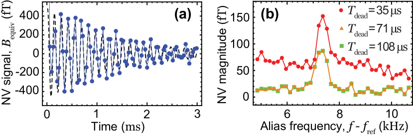
Figure 5: NV NQR recovery time. (a) Time-domain NV NQR signal of 4 grams of ${\rm NaNO}_{\rm 2}$ powder enclosed in a $Q\,{\approx}\,8$ resonant RF coil. The RF pulse was applied at $3608~{}{\rm kHz}$ for $200~{}{\rm\upmu s}$. A digital bandpass filter ($4.7\mbox{-}10.8~{}{\rm kHz}$) was applied for better visualization. (b) NV NQR spectrum (absolute value of Fourier transform) for three different deadtimes. $T_{\rm dead}$ is defined in Fig. 3(d).

IV.4 Sensor recovery time following an RF pulse

To detect NQR signals from samples with short dephasing times Verber et al. (1962); Augustine et al. (1998), a sensor with a short recovery time following an RF excitation pulse is desired. For inductive detection, the recovery time is determined by the resonant RF coil’s ring-down, and it can be ${\ll}100~{}{\rm\upmu s}$ for low-$Q$ coils. However, some non-inductive detectors like alkali-metal vapor magnetometers have significantly longer recovery times, ${\gtrsim}1~{}{\rm ms}$ Lee et al. (2006); Dhombridge et al. (2022). We hypothesized that the NV sensor’s recovery time should be limited by either the coil ring-down or the NV polarization time ($12~{}{\rm\upmu s}$ in our experiment), whichever is longer. To measure the recovery time, we used a 4-gram ${\rm NaNO}_{\rm 2}$ powder sample and a resonant RF coil with a loaded quality factor $Q\,{\approx}\,8$ (5). The smaller sample and lower $Q$ were chosen to test the limits of mass sensitivity and recovery time of our apparatus. Figure 5(a) shows the time-domain NV NQR signal following a $200\mbox{-}{\rm\upmu s}$ RF pulse (${\alpha}\,{\approx}\,119^{\degree}$). Fig. 5(b) shows the Fourier transform spectrum for three different “deadtimes”, computed by dropping the corresponding initial data points from the time-domain data in Fig. 5(a). For a deadtime of ${\sim}35~{}{\rm\upmu s}$, the NQR peak is still prominent above the background. The coil-detected signal exhibits a similar recovery time, suggesting that this timescale is limited by the coil ring-down time and not by properties of the NV centers.

The initial amplitude in Fig. 5(a), $B_{\rm equiv,i}\,{=}\,495\,{\pm}\,38~{}{\rm fT}$, is consistent with a modest amplification due to the resonant RF coil. Using Eq. 3, and correcting for the coil standoff from the sensor, the upper bound on the initial signal amplitude from the $4\mbox{-}\rm g$ sample is $B_{\rm equiv,i}\approx 760~{}{\rm fT}$ (Appendix G), which is only a factor of ${\sim}1.5$ larger than the experimental value.

IV.5 Spin-lock spin-echo spectroscopy

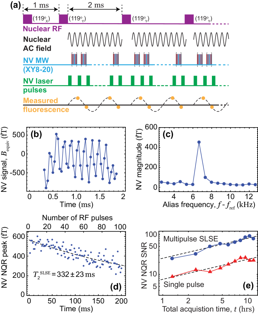
Figure 6: SLSE NV NQR signal. (a) Spin-Lock Spin-Echo (SLSE) pulse sequence. Following an initial RF pulse, one hundred echo pulses are applied every $2~{}{\rm ms}$. All RF pulses are applied at $3608~{}{\rm kHz}$ for $50~{}{\rm\upmu s}$ ($\alpha\approx 119^{\degree}$), and the initial pulse has a $90^{\degree}$ phase shift with respect to all the echo pulses. Meanwhile, a synchronized XY8-20 MW pulse sequence is applied to the NV centers, with $f_{\rm ref}=3600.07~{}{\rm kHz}$. The entire sequence is repeated every second. (b) Time-domain NV SLSE signal (coherent average of the first 20 echos) from the 21-g sample. (c) SLSE NQR spectrum obtained from the absolute value of the Fourier transform of data in (b). (d) SLSE signal magnitude as a function of the time passed since the first RF pulse. The fitted exponential decay constant is $T_{\rm 2}^{\rm SLSE}=332\pm 23~{}{\rm ms}$. (e) Signal-to-Noise Ratio (SNR) of NV NQR signals as a function of total acquisition time, $t$, for both SLSE and single-RF-pulse protocol. The dashed black lines are fits to a $\sqrt{t}$ dependence.

Nuclear spins in most room-temperature solids have the property $T_{\rm 2,\,nuc}^{\ast}\,{\ll}\,T_{\rm 1,\,nuc}$. This implies a low duty cycle for NQR readout, since $T_{\rm 2,\,nuc}^{\ast}$ limits the spin-precession acquisition time and $T_{\rm 1,\,nuc}$ bounds the re-thermalization time needed to repeat the sequence. One technique to increase the NQR readout duty cycle is to apply a Spin-Lock Spin-Echo (SLSE) pulse sequence Marino and Klainer (1977). In SLSE, Fig. 6(a), a series of phase-synchronized RF pulses are applied to extend the lifetime of the NQR signal out to a time $T_{2}^{\rm SLSE}\,{\gg}\,T_{\rm 2,\,nuc}^{\ast}$. Each echo pulse resets the phase of the nuclear spin precession, such that the NQR signals following each pulse can be coherently averaged together Marino and Klainer (1977); Cantor and Waugh (1980); Maricq (1986). Figures 6(b,c) show the NV-detected time-domain and frequency-domain SLSE signals from the 21-g sample averaged over the first 20 echos. A clear resonance at the expected NQR frequency ($f_{\rm alisas}+f_{\rm ref}=3606.7~{}{\rm kHz}$) is observed. Figure 6(d) shows the SLSE signal magnitude as a function of time since the first RF pulse. A fit to a single exponential decay reveals $T_{\rm 2}^{\rm SLSE}=332\pm 23~{}{\rm ms}$, a timescale that is consistent with previous studies Marino and Klainer (1977); Malone et al. (2011). Figure 6(e) shows the SLSE Signal-to-Noise Ratio (SNR) as a function of the total experimental acquisition time, $t$. The SNR of the single-RF-pulse measurement in Fig. 4 is also shown for comparison. In both cases, the SNR scales as $\sqrt{t}$, but the SLSE SNR is $\sim 3$ times greater. This is due to a combination of factors: the SLSE data has a ${\sim}3$-fold smaller NQR signal amplitude, but it has more than an order-of-magnitude higher readout duty cycle, and there was some additional RF noise in the single-pulse data that was not present in the SLSE measurement (Appendix H).

Discussion and conclusion

While this work realizes several benchmarks in the development of diamond quantum sensors, the present implementation of RF magnetometry and NQR detection operates far from fundamental limits. The diamond RF magnetometer sensitivity could be improved by illuminating a greater fraction of the diamond Clevenson et al. (2015), increasing the fluorescence collection efficiency Xu et al. (2019); Le Sage et al. (2012), optimizing the MW pulse sequence Zhou et al. (2020); Arunkumar et al. (2022), and increasing the flux concentrator enhancement factor Fescenko et al. (2020). Each of these improvements could plausibly provide a $\gtrsim 3$-fold improvement in sensitivity and taken together might allow a sensitivity $\lesssim 1~{}{\rm fT\,s^{1/2}}$, provided the flux concentrator’s magnetic noise remains sufficiently low Lee and Romalis (2008). Magnetic fields from localized samples may also be further enhanced by providing an additional flux return path using a closed cylinder or C-shaped ferrite clamp Kim and Savukov (2016).

To improve NQR detection, it is tempting to leverage the resonant-induction amplification method introduced here and increase the coil $Q$, see Eq. (3). However, the Johnson noise in the coil is also resonantly amplified and must be considered. The rms Johnson magnetic noise inside an impedance-matched solenoidal coil on resonance Qiu et al. (2007) is:

$$\eta_{\rm J}\,{\approx}\,\sqrt{\frac{2\,k_{\rm B}\,T\,\mu_{\rm c}\,Q}{\pi\,f_{0}\,V_{\rm c}}},$$ (4)

where $k_{\rm B}$ is the Boltzmann constant, $T$ is the temperature, $\mu_{\rm c}$ is the permeability inside the coil, and $f_{0}$ is the coil’s resonance frequency. When using a high-Q RF coil wrapped around the sample, the SNR of NQR detection is fundamentally limited by Johnson noise, regardless of the mode of detection. Assuming $f_{0}=f_{\rm nqr}$ and $\mu_{\rm c}=\mu_{0}$, where $\mu_{0}$ is the vacuum permeability, and neglecting nuclear-spin dephasing and experimental dead times, the Johnson-noise-limited SNR is given by Eqs. (3),(4) as Hoult and Richards (1976):

$${\rm SNR_{J}}\approx\sqrt{\frac{\pi\mu_{0\,}Qf_{\rm nqr}}{4V_{\rm c\,}k_{\rm B\,}T}}\frac{m_{\rm s}}{\rho_{\rm s}}M_{0}.$$ (5)

Using parameters from the experiment (5), we find ${\rm SNR_{J}}\approx 210~{}{\rm Hz^{1/2}}$ for the 4-g coil and ${\rm SNR_{J}}\approx 1020~{}{\rm Hz^{1/2}}$ for the 21-g coil. These values are ${\sim}2$ orders of magnitude higher than the SNR in our experiments (1), but they represent an upper bound for future optimization. In either case, increasing $Q$ can improve the SNR in NQR experiments. For Johnson-noise-limited detection, ${\rm SNR_{J}}\propto\sqrt{Q}$, Eq. (5). If the noise floor is not yet limited by Johnson noise, as in our experiments (2), ${\rm SNR}\propto Q$, since $M_{\rm eff}$ still scales linearly with $Q$, Eq. (3). However, in both cases, higher $Q$ is likely to result in a longer recovery time, which is problematic for some applications Verber et al. (1962); Augustine et al. (1998); Malone et al. (2020). Ultimately, the benefits of the resonant-induction amplification method are limited, as the SNR upper bound is the same for both diamond RF magnetometer and inductive-coil detection, and the method may not be compatible with remote detection.

For remote NQR detection, an optimized diamond RF magnetometer is more likely to offer a clear advantage over inductive-coil detection. Consider the case where a low-$Q$ RF excitation loop is located sufficiently far from the sample that resonant-induction amplification can be neglected (3). Suppose the ferrite-cones diamond RF magnetometer in the present experiment was replaced by a Johnson-noise-limited coil of equivalent volume ($V_{c}=1.5~{}{\rm cm^{3}}$) with $Q=10$. The equivalent magnetic sensitivity of such a sensor is $\eta_{\rm J}/Q=8~{}{\rm fT_{rms}\,Hz^{-1/2}}$, see Eq. (4). An order-of-magnitude improvement in diamond RF magnetometer sensitivity would already provide a superior SNR. Such a device could find application as a non-contact detector of pharmaceutical compounds, such as synthetic opioids like fentanyl, which require high sensitivity and a short recovery time Malone et al. (2020). Beyond NQR spectroscopy, our device may also be used in applications such as magnetic induction tomography Chatzidrosos et al. (2019); Rushton et al. (2022), underwater communication Gerginov et al. (2017); Deans et al. (2018), or the search for exotic spin interactions Jackson Kimball et al. (2016); Chu et al. (2022); Liang et al. (2022).

In summary, we demonstrated a broadband ($0.07{-}3.62~{}{\rm MHz}$) ferrite-cones diamond RF magnetometer with a sensitivity of ${\sim}70~{}{\rm fT\,s^{1/2}}$ at $0.35~{}{\rm MHz}$. The magnetometer was used to detect the $3.6~{}{\rm MHz}$ NQR signal of ${}^{14}{\rm N}$ from room temperature ${\rm NaNO}_{\rm 2}$ powder samples. The short recovery time in our device after RF excitation pulse, ${\sim}35~{}{\rm\upmu s}$, may offer advantages over other sensitive magnetometers for NQR spectroscopy.

Appendix Appendix A

Experimental setup

The apparatus used here, shown in Fig. 1(a), was adapted from the one presented in Ref. Fescenko et al. (2020). Here we provide additional information, with a focus on the changes that were implemented for RF magnetometry. An acousto-optic modulator (Brimrose TEM-85-10-532), driven at $81~{}{\rm MHz}$ by an RF signal generator (RF-Consultant TPI-1001-B), is used to gate a continuous-wave 532 nm green laser beam (Lighthouse Photonics Sprout D-5W) and produce $12\mbox{-}{\rm\upmu s}$ laser pulses. Following the AOM, a half-wave plate (Thorlabs WPH10ME-633) is used to adjust the laser beam’s polarization. The laser beam is then focused onto the edge facet of a diamond membrane using a 1-inch diameter aspheric condenser lens (${\rm NA}\,{=}\,0.79$, Thorlabs ACL25416U-B). The same condenser lens is used to collect the NV fluorescence. The fluorescence is spectrally filtered by a dichroic mirror (Thorlabs DMLP567R) and a $650~{}{\rm nm}$ long-pass filter (Thorlabs FELH0650). Finally, it is focused onto the “fluorescence channel” of the photodetector using a 2-inch diameter lens (Thorlabs ACL50832U-B).

A two-channel balanced photodetector (Thorlabs PDB210A) with a fixed gain $G=175~{}{\rm kV/A}\approx 1.1\times 10^{24}~{}{\rm V/(photoelectron/s)}$ and a 3-dB bandwidth of ${\rm DC}{-}1~{}{\rm MHz}$ is used to record the NV fluorescence signal. A small portion of the laser beam is picked off prior to the condenser lens and is directed to the “laser channel” of the photodetector for balanced detection.

The laser beam’s peak power is measured before the condenser lens (but after the pick-off) to be ${\sim}250~{}{\rm mW}$. We estimate the peak power entering the diamond to be ${\sim}200~{}{\rm mW}$, after taking into account the ${\sim}80\%$ transmission of the aspheric condenser at 532 nm wavelength. Using a camera imaging system, the full-width-at-half-maximum (FWHM) spot diameter of the laser beam on the diamond face was estimated to be ${\sim}35~{}{\rm\upmu m}$. The effective sensing volume, $V_{\rm sen}$, is taken as the product of the excitation beam area, ${\sim}\pi\times(35~{}{\rm\upmu m}/2)^{2}$ and the optical path length in the diamond, ${\sim}300~{}{\rm\upmu m}$.

The diamond membrane used here was created from a natural-isotopic-abundance diamond substrate. grown by chemical-vapor deposition, with an initial nitrogen concentration $[{\rm N}]\,{\approx}\,20~{}{\rm ppm}$. The diamond was irradiated with 2-MeV electrons at a dose of ${\sim}10^{18}~{}{\rm cm^{-2}}$, and then it was annealed in a vacuum furnace at $800\mbox{-}1100\,^{\circ}{\rm C}$ to form NV centers. The diamond properties, irradiation, and annealing procedures are similar to that described in Ref. Smits et al. (2019). The diamond was subsequently cut and polished into a (100)-oriented membrane with dimensions ${\sim}300\times 300\times 35~{}{\rm\upmu m^{3}}$.

A ${\sim}1$-cm thick rectangular aluminum shield with $18.4{\times}18.4{\times}30.8~{}{\rm cm^{3}}$ dimensions is placed around the magnetometer apparatus to reduce RF interference. A permanent magnet placed outside of the Al-shield, ${\sim}65~{}{\rm cm}$ above the ferrite cones, is used to compensate the laboratory’s ambient magnetic field and to apply weak bias magnetic fields, $B_{0}=2\mbox{-}10~{}{\rm\upmu T}$, approximately along the $z$-axis. A vector magnetometer (Twinleaf VMR018) is used to map the bias magnetic field at the location of the cones. The field components along the $x$ and $y$ axes are minimized by moving the magnet around.

An I/Q-modulated microwave (MW) signal generator (Rohde$\,{\&}\,$Schwarz SMU200A) is used to drive the NV electron spin transitions in the $2.7\mbox{-}3.0~{}{\rm GHz}$ frequency range. DC voltages, gated by a pair of TTL-controlled switches, are used to modulate the MW carrier’s phase, via the generator’s analog I/Q modulation port. A third switch is used to gate the MW amplitude on a ${\sim}10~{}{\rm ns}$ timescale. Then, the MW pulses are passed through an amplifier (Mini-Circuits ZHL-16W-43-S+) and circulator, and the output is connected to a one-and-a-half-turn copper loop (AWG38). This loop is wound around one of the ferrite cones and positioned ${\sim}100~{}{\rm\upmu m}$ above the gap between the cones. For the measurements without the cones, a copper wire placed on top of the diamond, parallel to the excitation beam, was used to drive the NV spin transition.

A waveform signal generator (Teledyne LeCroy Wavestation 2012) is used as a source for low-frequency RF signals. One of its channels is used to create sinusoidal RF test signals. The output of this channel is connected to a pair of rectangular wire loops with ${\sim}1.5{\times}3.0{\times}1.6~{}{\rm cm^{3}}$ dimensions placed around the diamond-cones assembly. The rectangular loop pair has a low enough impedance that it produces RF magnetic fields with a relatively constant amplitude (at constant applied voltage amplitude) from $0\mbox{-}4~{}{\rm MHz}$ (see 1). The dimensions of the rectangular loop pair are still large enough that they produce magnetic fields that are approximately uniform over the region of the two ferrite cones.

The entire experiment is controlled by a TTL pulse card (SpinCore PBESR-PRO-500) with an onboard ovenized crystal oscillator. The differential photodetector signal is digitized by the analog input of a data acquisition (DAQ) card (NI USB-6361). The DAQ sampling is synchronized to the overall pulse sequence through a trigger pulse from the TTL pulse card. External ovenized crystal oscillators are used to stabilize the internal clocks of the DAQ and RF signal generator.

Appendix Appendix B

Diamond RF magnetometer sensitivity

1 Photoelectron shot noise in balanced detection

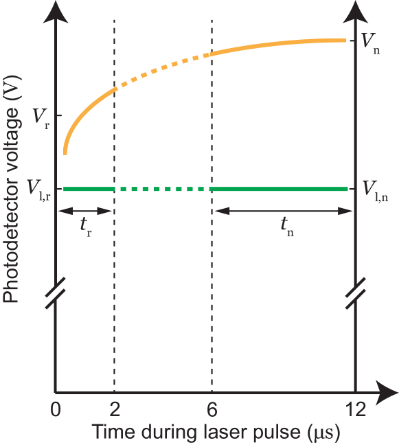
Figure A7: Definition of variables for balanced detection and normalization. Schematic of photodetector voltage traces in the fluorescence channel (orange line) and laser channel (green line) during a single laser pulse. $V_{\rm r}$ and $V_{\rm l,r}$ are the average voltages during the readout window (duration: $t_{\rm r}$), and $V_{\rm n}$ and $V_{\rm l,n}$ are the average voltages during the normalization window (duration: $t_{\rm n}$).

The minimum detectable magnetic field of a magnetometer can be defined as:

$$\delta B_{\rm min}=\frac{\delta S_{\rm min}}{\frac{\partial S}{\partial B}},$$ (AII-1)

where $S$ is the field-dependent signal measured by the magnetometer and $\delta S_{\rm min}$ is the minimum noise of a single measurement. In our diamond RF magnetometer, $S$ is the difference in balanced photodetector voltages averaged over two time windows–a “readout window” and a “normalization window”, see Fig. A7. It is given by:

$$\begin{split}S=V_{\rm r}(B,t)-V_{\rm l,r}-(V_{\rm n}-V_{\rm l,n})~{}~{}~{}~{}~{}~{}~{}~{}&\\ =G\bigl{[}\frac{N_{\rm r}(B,t)}{t_{\rm r}}-\frac{N_{\rm l,r}}{t_{\rm r}}-\frac{N_{\rm n}}{t_{\rm n}}+\frac{N_{\rm l,n}}{t_{\rm n}}\bigr{]}.\end{split}$$ (AII-2)

In Eq. (AII-2), the quantity $V_{\rm r}(B,t)-V_{\rm l,r}$ is the average photodetector voltage during the readout window of duration $t_{\rm r}$, $N_{\rm r}$ is the equivalent number of photoelectrons detected on the fluorescence channel during the readout window, and $N_{\rm l,r}$ is the corresponding number on the laser channel. The quantity $V_{\rm n}-V_{\rm l,n}$ is the average photodetector voltage during the normalization window of duration $t_{\rm n}$, $N_{\rm n}$ is the equivalent number of photoelectrons detected on the fluorescence channel during the normalization window, and $N_{\rm l,n}$ is the corresponding number on the laser channel. To a good approximation, the only photodetector voltage that depends on magnetic field is $V_{\rm r}(B,t)$–the other voltages that comprise $S$ are independent of magnetic field.

In the synchronized readout scheme, Fig. 1(b), the signal is sampled at times $t=P\,\tau_{\rm sample}$, with $P$ being a non-negative integer, where $t$ is defined as the time at the beginning of the first $\pi/2$ pulse in an XY8-$N$ sequence. If an AC cosine magnetic field with amplitude $B$ and frequency $f$ is applied along the sensing axis in our NV-cones magnetometer, $V_{\rm r}(B,t)$ is modulated as:

$$\begin{split}V_{\rm r}(B,t)~{}{=}~{}V_{0}\bigl{[}1\,&+\,C\,\sin{(\frac{4}{\sqrt{3}}\,\epsilon\,\gamma_{\rm nv}\,B\,\tau_{\rm tot})}\times\\ &\cos{(2\pi(f-f_{\rm ref})\,t+\phi_{0})}\bigr{]}.\end{split}$$ (AII-3)

In Eq. (AII-3), $V_{0}\approx 30~{}{\rm V}$ is the mean fluorescence-channel voltage, $C$ is the effective fluorescence contrast of the XY8-$N$ sequence, $\epsilon$ is the flux-concentrator enhancement factor, $\tau_{\rm tot}$ is the total NV phase accumulation time during an XY8-$N$ sequence, $f_{\rm ref}$ is the reference frequency, and $\phi_{0}$ is the phase of the cosine AC field at $t=0$ (the first $\pi/2$ pulse of the first XY8-$N$ sequence).

For $f=f_{\rm ref}$ and $\phi_{0}=0$, a straightforward inspection of Eq. (AII-3) reveals that the magnetometer response to small amplitude RF fields ($\gamma_{\rm nv}B\tau_{\rm tot}\ll 1$) is given by:

$$\frac{\partial S}{\partial B}=\frac{\partial V_{\rm r}}{\partial B}\approx\frac{4}{\sqrt{3}}V_{0}\,C\,\epsilon\,\gamma_{\rm nv}\,\tau_{\rm tot}.$$ (AII-4)

Eq. (AII-4) turns out to be valid for all values of $\phi_{0}$ and $f$ as long as $(f-f_{\rm ref})\,\tau_{\rm sample}<0.5$. Due to the constraints in the definition of $f_{\rm ref}$, this is equivalent to saying that Eq. (AII-4) is valid for test field frequencies that fall within the frequency-domain filter-function response of the XY8-$N$ sequence Glenn et al. (2018); Smits et al. (2019).

The noise in the processed signal $S$ is theoretically limited by photoelectron shot noise. Using the definition of $S$ in Eq. (AII-2), the minimum detectable noise of a single readout, $\delta S_{\rm min}$, can be written in root-mean-squared (rms) voltage units as:

$$\delta S_{\rm min}=G\sqrt{\frac{N_{\rm r}}{t_{\rm r}^{2}}+\frac{N_{\rm l,r}}{t_{\rm r}^{2}}+\frac{N_{\rm n}}{t_{\rm n}^{2}}+\frac{N_{\rm l,n}}{t_{\rm n}^{2}}}.$$ (AII-5)

In the small contrast regime that our experiments operate in, $C\ll 1$, the detected photoelectron rates in the fluorescence and laser channels are approximately the same for both readout and normalization windows:

$$\frac{N_{\rm n}}{t_{\rm n}}\approx\frac{N_{\rm l,r}}{t_{\rm r}}\approx\frac{N_{\rm l,n}}{t_{\rm n}}\approx\frac{N_{\rm r}}{t_{\rm r}}=\frac{n_{\rm nv}V_{\rm sen}\phi}{t_{\rm r}}=\frac{V_{0}}{G},$$ (AII-6)

where $n_{\rm nv}$ is the NV concentration, $V_{\rm sen}$ is the illuminated NV sensor volume, and $\phi$ is the probability of detecting a photoelectron per NV center in a single readout. Inserting Eq. (AII-6) into Eq. (AII-5), the noise becomes:

$$\delta S_{\rm min}=\frac{G}{t_{\rm r}}\sqrt{2\,(1+\frac{t_{\rm r}}{t_{\rm n}})\,n_{\rm nv}V_{\rm sen}\phi}=\frac{G\xi}{t_{\rm r}}\sqrt{n_{\rm nv}V_{\rm sen}\phi},$$ (AII-7)

where $\xi=\sqrt{2\,(1+t_{\rm r}/t_{\rm n})}$ accounts for the extra photoelectron noise due to the balanced detection and normalization procedure.

Inserting Eqs. (AII-4), (AII-6), and (AII-7) into Eq. (AII-1), the minimum detectable RF magnetic field from a single readout is:

$$\delta B_{\rm min}\approx\frac{\sqrt{3}\,\xi}{\epsilon}\frac{1}{4\,\gamma_{\rm nv}\,C\,\tau_{\rm tot}\sqrt{n_{\rm nv}\,V_{\rm sen}\,\phi}}.$$ (AII-8)

For successive NV readouts with repetition time $\tau_{\rm sample}$ and duty cycle $\delta=\tau_{\rm tot}/\tau_{\rm sample}$, the photoelectron-shot-noise limited sensitivity in the diamond RF magnetometer is given by:

$$\eta_{\rm psn}=\delta B_{\rm min}\sqrt{\tau_{\rm sample}}\approx\frac{\sqrt{3}\,\xi}{\epsilon\,\sqrt{\delta}}\frac{1}{4\,\gamma_{\rm nv}\,C\sqrt{n_{\rm nv}\,V_{\rm sen}\,\phi\,\tau_{\rm tot}}},$$ (AII-9)

which is the expression given in Eq. (1) of the main text.

Figure A8: NV test field saturation curve. NV test signal fluorescence magnitude $V_{\rm nv}$ without the cones as a function of the applied RF voltage to the test loop, $V_{\rm test}$. The RF test fields were applied at $0.35~{}{\rm MHz}$ frequency and their projections along the $z$-axis were detected by the NV centers in diamond. Here, an XY8-4 pulse sequence with $76\mbox{-}{\rm ns}$ MW $\pi$-pulse length and $\tau\,{=}\,684~{}{\rm ns}$ was used to detect the test signals. The vertical dashed line is the magnetic field amplitude that leads to an NV total phase accumulation of $\pi/2~{}{\rm radians}$ during a single XY8-4 sequence. The solid black line is a fit to an absolute-value-of-sine function, Eq. (AIII-10). From the fit, the scaling factor between the applied RF voltage and the NV detected magnetic field along the $z$-axis is found to be $\kappa\,{=}\,0.307\pm 0.004~{}{\rm\upmu T_{rms}/V_{pp}}$.

For sensitivity measurements in Fig. 2, the readout window duration was $t_{\rm r}=2~{}{\rm\upmu s}$ and the normalization window duration was $t_{\rm n}=6~{}{\rm\upmu s}$. For all NQR measurements, we used $t_{\rm r}=1.5~{}{\rm\upmu s}$ and $t_{\rm n}=5~{}{\rm\upmu s}$. In either case, $\xi\approx 1.6$ and the calculated values for $\eta_{\rm psn}$ were similar.

2 Comparing to experimental sensitivity

The photoelectron-shot-noise-limited sensitivity formulas given in Eqs. (1) and (AII-9) describe the standard deviation of magnetometer signals in the time-domain for successive $1\mbox{-}{\rm s}$ measurements. In experiments, the magnetic field sensitivity was reported as the average noise floor of the NV fluorescence signal in the frequency-domain. It was obtained by taking the mean noise floor in spectra computed from the absolute value of the Fourier transform of $1\mbox{-}{\rm s}$ NV signals. For white noise, it can be shown that the standard deviation in the time domain (the theory method) is a factor of ${\sim}1.25$ smaller than the mean of the absolute value of the Fourier transform (experimental method). Incorporating this factor in Eq. (1), the photoelectron-shot-noise limited sensitivity of our ferrite-cones-diamond magnetometer would be ${\sim}38~{}{\rm fT_{rms}\,s^{1/2}}$ using the frequency-domain-analysis method.

Table A1: Calibration factors and enhancement for different test-field frequencies. The values for $\tau$, $N$, $\pi$-pulse length, and $\tau_{\rm sample}$ are for when the cones were assembled around the diamond. There are ${\sim}1\%$ fit uncertainty and ${\sim}8\%$ day-to-day systematic variation on the reported values for $\kappa$ and $\kappa_{\rm m}$. For each test frequency, the enhancement factor ($\epsilon$) was estimated by dividing the scaling factor with the cones by the value without them.

Test frequ-ency (MHz)	$\boldsymbol{\tau}$ (ns)	$\boldsymbol{N}$	${\pi}$-pulse length (ns)	$\boldsymbol{\tau_{\rm sample}}$ (${\rm\upmu s}$)	$\boldsymbol{\kappa}$ with cones (${\rm\upmu T_{rms,gap}/V_{pp}}$)	$\boldsymbol{\kappa_{\rm m}}$ with cones (${\rm\upmu T_{rms,gap}/V_{pp}}$)	$\boldsymbol{\kappa}$ no cones (${\rm\upmu T_{rms}/V_{pp}}$)	$\boldsymbol{\kappa_{\rm m}}$ no cones (${\rm\upmu T_{rms}/V_{pp}}$)	Enhanc-ement, $\epsilon$
0.07	3548	1	44	73.07	101	101	0.318	0.315	${319\pm 3}$
0.10	2478	1	44	60.61	84	84	0.310	0.306	${273\pm 4}$
0.20	1226	2	48	55.28	82	81	0.300	0.292	${275\pm 4}$
0.35	698	4	48	60.93	96	92	0.307	0.291	${314\pm 3}$
0.70	332	7	48	55.69	102	95	0.346	0.313	${299\pm 9}$
1.00	224	8	52	47.09	110	98	0.359	0.310	${311\pm 10}$
1.51	140	8	52	35.90	128	108	0.393	0.312	${336\pm 20}$
2.02	96	10	56	34.75	138	107	0.435	0.316	${328\pm 21}$
2.50	68	13	64	35.62	173	118	0.486	0.321	${362\pm 12}$
3.12	48	16	64	35.22	184	111	0.578	0.332	${326\pm 16}$
3.62	56	20	26	36.73	${\sim}130$	${\sim}106$

Appendix Appendix C

RF test field calibration and ferrite enhancement

1 RF test field calibration

In the main text, the NV fluorescence processed signal, Eq. (AII-2), was calibrated to a known applied AC magnetic field. We performed the test-field calibration with two methods: (i) using the theoretical signal response of the NV centers themselves, with and without the cones, and (ii) independent measurements of the frequency dependence of inductive pick-up in a wire loop.

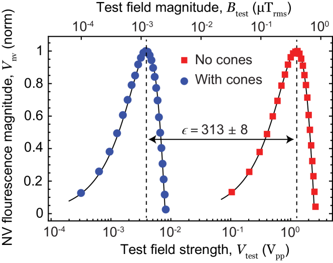
Figure A9: RF calibration with and without cones. Normalized NV test signal fluorescence magnitude as a function of the applied RF voltage to the test loop with (blue circles) and without (red squares) the cones. RF test fields were applied at $0.35~{}{\rm MHz}$ frequency and XY8-4 readout sequences with $\tau\,{=}\,698~{}{\rm ns}$ and $684~{}{\rm ns}$ were used to detect their $z$-axis projections inside the diamond with and without the cones, respectively. The NV test signal magnitudes are fit to Eq. (AIII-10) (solid black lines), revealing the scaling factor $\kappa\,{=}\,96\pm 2~{}{\rm\upmu T_{rms,gap}/V_{pp}}$ with the cones and $\kappa\,{=}\,0.307\pm 0.004~{}{\rm\upmu T_{rms}/V_{pp}}$ without them. From the ratio of these scaling factors, the RF field enhancement provided by the ferrite cones was estimated to be $\epsilon\,{=}\,313\pm 8$ at $0.35~{}{\rm MHz}$ frequency.

For method (i), an RF test signal, with a peak-to-peak voltage $V_{\rm test}$ and frequency $f_{\rm test}$, is applied to the rectangular wire loops placed around the diamond when the ferrite cones were absent ($\epsilon=1$). For each value of $f_{\rm test}$, the amplitude $V_{\rm test}$ is varied and the NV signal is recorded at each value of $V_{\rm test}$. From Eq. (AII-3), the NV test signal fluorescence magnitude $V_{\rm nv}$ (in rms voltage units) is given by:

$$V_{\rm nv}~{}{=}~{}V_{\rm max}\,|\sin\,(4\,\sqrt{\frac{2}{3}}\,\kappa\,V_{\rm test}\,\gamma_{\rm nv}\,\tau_{\rm tot})|,$$ (AIII-10)

where $V_{\rm max}=V_{0}\,C/\sqrt{2}$ is the maximum NV test signal magnitude, $\tau_{\rm tot}$ is the NV phase accumulation time, and $\kappa=B_{\rm test}/V_{\rm test}$ is the scaling factor which provides us with the calibration. Note that there are two plausible definitions of $\tau_{\rm tot}$ and each results in a slightly different value of $\kappa$. If we assume $\tau_{\rm tot}$ is the interval between $\pi/2$ pulses in an XY8-$N$ sequence, excluding the time for $\pi$-pulses Smits et al. (2019), then $\tau_{\rm tot}=16N\tau$, and we use the variable $\kappa$ for the scaling factor. If $\tau_{\rm tot}$ is the entire interval between $\pi/2$ pulses in an XY8-$N$ sequence Glenn et al. (2018), then $\tau_{\rm tot}=8N(2\tau+t_{\rm\pi,mw})=4N/f_{\rm test}$, where $t_{\rm\pi,mw}$ is the MW $\pi$-pulse length, and we use $\kappa_{\rm m}$ for the scaling factor.

Figure A8 shows the NV fluorescence signal magnitude without the cones versus $V_{\rm test}$. Here, $f_{\rm test}=0.35~{}{\rm MHz}$, and an XY8-4 pulse sequence with $t_{\rm\pi,mw}=76~{}{\rm ns}$ and $\tau=684~{}{\rm ns}$ was used to detect the test signals. Fitting the data to Eq. (AIII-10) reveals the scaling factor $\kappa\,{=}\,0.307\pm 0.004~{}{\rm\upmu T_{rms}/V_{pp}}$. The same procedure was applied to the setup with the cones in place ($\kappa=B_{\rm gap}/V_{\rm test}$), and the results with and without cones are shown in Fig. A9. With the cones present, the maximum of the NV signal occurs at a ${\sim}313$ times lower test field amplitude. This is due to the flux-concentrator enhancement of the RF test field, and the ratio of the fitted response curves provides a measure of $\epsilon$, see 2.

We repeated the same process for different test frequencies. For each frequency, $\tau$, $t_{\rm\pi,mw}$, and $N$ were adjusted to maximize the NV test signal. Table A1 shows the resulting calibration factors, $\kappa$ and $\kappa_{\rm m}$, with and without the cones. Figure A10(a) shows a plot of the fitted values of $\kappa$ and $\kappa_{\rm m}$ with and without cones as a function of $f_{\rm test}$. For $f_{\rm test}\lesssim 1~{}{\rm MHz}$, both definitions of calibration are approximately constant and consistent with $\epsilon\approx 300$. For higher frequency, $\kappa$ begins to increase both with and without cones. An increase in field strength as a function of $f_{\rm test}$ was unexpected–if anything, we expected a decrease due to the finite inductance of the test-loop coil. While a full spin dynamics simulation is beyond the scope of this study, this behavior may imply that NV spin precession during the MW $\pi$-pulses should not be neglected when estimating the NV phase accumulation. To provide an independent check of the test-field frequency dependence, we turned to calibration method (ii).

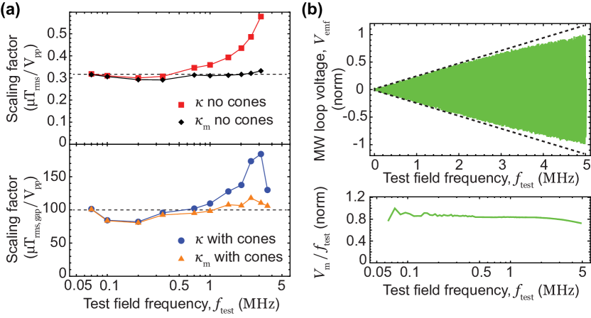
Figure A10: Frequency-dependent calibration of the test field. (a) Scaling factor $\kappa$ and its modified version $\kappa_{\rm m}$ versus the test field frequency for with (bottom) and without (top) the cones. The dashed black lines indicate the scaling factors we applied to calibrate the diamond RF magnetometer for all frequencies throughout the main text. (b) Normalized induced voltage in the MW loop versus frequency of the RF carrier applied to the rectangular test loop. The induced voltage amplitude increases linearly with frequency consistent with Faraday’s law (dashed black lines) up to ${\sim}3~{}{\rm MHz}$. This measurement was done with the diamond-cones assembly inside the test loop. The solid green line (bottom) shows the frequency-normalized induced voltage amplitude in the MW loop.

For calibration method (ii), we studied the frequency response of the rectangular test loops using an inductive pickup loop. An RF carrier with $5~{}{\rm V_{pp}}$ amplitude was applied to the test loops, with the diamond-cones assembly in place, and the RF carrier frequency, $f_{\rm test}$, was swept linearly with rate $\alpha_{\rm s}\,{\approx}\,200~{}{\rm MHz/s}$ from $1~{}{\rm kHz}$ to $5~{}{\rm MHz}$. The oscillating pickup voltage in the small wire loop wrapped around one of the cones (that is usually used for MW delivery) was recorded by an oscilloscope (Yokogawa DL9140L). Figure A10(b, top) shows the MW loop voltage, $V_{\rm emf}$, as a function of $f_{\rm test}$. As expected from Faraday’s law, $V_{\rm emf}$ increases linearly with frequency for $f_{\rm test}\lesssim 3~{}{\rm MHz}$. At higher frequency, the slope gradually reduces, presumably due to a rise in impedance of the inductive test-field loops.

Table A2: XY8-$\boldsymbol{N}$ sensitivity vs test field frequency. The sensitivities with and without the cones were obtained by applying a uniform RF test field with magnitude $B_{\rm test}\,{\approx}\,100~{}{\rm pT_{rms}}$ along the $z$-axis. The effective fluorescence contrast $C$ with the cones was obtained from Eq. (AIV-11) assuming $\epsilon\,{=}\,316$ for all test frequencies. For each test frequency, the average noise floor of the absolute Fourier transform spectrum was extracted from a ${\sim}100\mbox{-}{\rm Hz}$ wide region of the spectrum that did not contain spurious noise spikes.

Test frequ-ency (MHz)	$\boldsymbol{\tau}$ (ns)	$\boldsymbol{N}$	${\pi}$-pulse length (ns)	$\boldsymbol{\tau_{\rm sample}}$ (${\rm\upmu s}$)	$\boldsymbol{C}$	Sensitivity with cones (${\rm fT_{rms}\,s^{1/2}}$)	Sensitivity no cones (${\rm pT_{rms}\,s^{1/2}}$)
0.07	3548	1	44	73.07	0.002	${200\pm 13}$	${60.4\pm 3.6}$
0.10	2478	1	44	60.61	0.004	${150\pm 8}$	${28.6\pm 1.6}$
0.20	1226	2	48	55.28	0.006	${89\pm 4}$	${19.3\pm 1.2}$
0.35	698	4	48	60.93	0.009	${73\pm 4}$	${18.5\pm 0.9}$
0.70	332	7	48	55.69	0.007	${106\pm 6}$	${21.7\pm 1.4}$
1.00	224	8	52	47.09	0.008	${105\pm 5}$	${20.6\pm 1.1}$
1.51	140	8	52	35.90	0.010	${119\pm 8}$	${22.6\pm 1.2}$
2.02	96	10	56	34.75	0.009	${128\pm 6}$	${25.6\pm 1.4}$
2.52	86	13	26	35.27	0.013	${172\pm 8}$	${26.7\pm 1.5}$
3.09	68	16	26	35.34	0.009	${229\pm 8}$	${49.3\pm 3.2}$
3.62	56	20	26	36.73	0.010	${202\pm 8}$

The data set in Fig. A10(b, top) was divided into $10~{}{\rm kHz}$ segments, and each segment was fit to a function $V_{\rm emf}\,{=}\,V_{\rm m}\sin{(2\pi\,f_{\rm test}^{2}/\alpha_{\rm s}+\phi_{\rm i})}$ to extract the amplitude $V_{\rm m}$ and initial phase $\phi_{\rm i}$ of the oscillation. The induced voltage’s amplitude divided by frequency, $V_{\rm m}/f_{\rm test}$, versus the test field frequency is plotted in Fig. A10(b, bottom). The response is approximately flat in the $0.07\mbox{-}3.6~{}{\rm MHz}$ frequency range studied in our experiments.

The combined observation from both calibration methods is that, to a decent approximation, the RF test field amplitude is independent of frequency in the $0.07\mbox{-}3.6~{}{\rm MHz}$ range studied here. Thus, we applied constant scaling factors, $\kappa_{\rm m}\,{=}\,0.316~{}{\rm\upmu T_{rms}/V_{pp}}$ for data without the cones and $\kappa_{\rm m}\,{=}\,100~{}{\rm\upmu T_{rms,gap}/V_{pp}}$ for data with cones, for all frequencies $f_{\rm test}$ throughout the main text. These values are denoted as dashed black lines in Fig. A10(a). The only exception is the data in Fig. 2(d), where we use the measured values in Tab. A1 to explicitly show the small fluctuations ($\lesssim 10\%$) of enhancement factor as a function of frequency.

2 Ferrite RF field enhancement measurement

For each test frequency, the RF enhancement provided by the ferrite cones is estimated as the ratio of the scaling factor with the cones to the value without them. Two enhancement factors were obtained for each frequency, one from the $\kappa$-ratio and another from the $\kappa_{\rm m}$-ratio, and their mean value as well as deviation from the mean are reported in Tab. A1 and plotted in Fig. 2(d).

Appendix Appendix D

Frequency-dependence of magnetometer sensitivity

In Fig. 2(e) of the main text, we present the sensitivity of the diamond RF magnetometer as a function of test frequency with and without the ferrite cones. For these measurements, a sinusoidal RF carrier with a small voltage amplitude $V_{\rm test}\,{\approx}\,316~{}{\rm\upmu V_{pp}}$ was applied to the test field loops. This small voltage was provided by inserting a 30-dB attenuator in the output of the RF signal generator. Based on calibration measurements (Appendix C), this produced a uniform magnetic test field with magnitude $B_{\rm test}\,{\approx}\,100~{}{\rm pT_{rms}}$ along the $z$-axis for the $0.07\mbox{-}3.6~{}{\rm MHz}$ frequency range.

Table A2 summarizes the XY8-$N$ setting parameters for each test frequency when the cones were arranged around the diamond, along with the experimentally-determined sensitivities with and without the cones. At each frequency setting, $\tau$, $N$, and the microwave $\pi$-pulse length were optimized to give the best sensitivity. Then, the magnetometer signal was recorded for $100~{}{\rm s}$ with and without the ferrite cones. Each $100\mbox{-}\rm{s}$ data set was divided into one hundred $1\mbox{-}\rm{s}$ segments, and a spectrum was obtained for each segment by taking the absolute value of the Fourier transform. Then the NV test signal’s fluorescence magnitude ($V_{\rm nv}$) as well as the mean noise floor were extracted for each spectrum. The noise band was selected within a spike-free $100~{}{\rm Hz}$ wide band. Typically, we chose the band at a relatively high alias frequency to avoid picking up any low-frequency drifts of the NV fluorescence signal. The sensitivity for each frequency is reported as the mean value of the average noise floors for one hundred segments, see Fig. 2(e) and Table A2. The error bar on the reported sensitivity is the standard deviation of the 100 sensitivity measurements.

In Fig. 2(b) of the main text, the frequency band used to calculate noise was $3.0{-}3.7~{}{\rm kHz}$ for the magnetic spectrum without the cones (red), $2.85{-}3.10~{}{\rm kHz}$ for the spectrum with the cones (blue), and $2.8{-}3.0~{}{\rm kHz}$ for the spectrum with the cones when the MW frequency was detuned (green). The bands used to calculate the noise are different in each data set to avoid including the small spikes that appear in different regions of the spectrum (presumably due to RF interference) from time to time.

In a small field approximation, the contrast can be derived from Eq. (AII-3) as:

$$C~{}{\approx}~{}\frac{\sqrt{3}\,V_{\rm nv}}{4\,\epsilon\,B_{\rm test}\,\gamma_{\rm nv}\,\tau_{\rm tot}\,V_{0}}.$$ (AIV-11)

For each test frequency, we used the observed value of $V_{\rm nv}$ and Eq. (AIV-11) to estimate $C$ for each test frequency, Table A2, assuming $B_{\rm test}\,{=}\,100~{}{\rm pT_{rms}}$ and $\epsilon\,{=}\,316$. A typical value of the contrast obtained in our setup for $f_{\rm test}=0.35~{}{\rm MHz}$ is $C\,{\approx}\,0.01$.

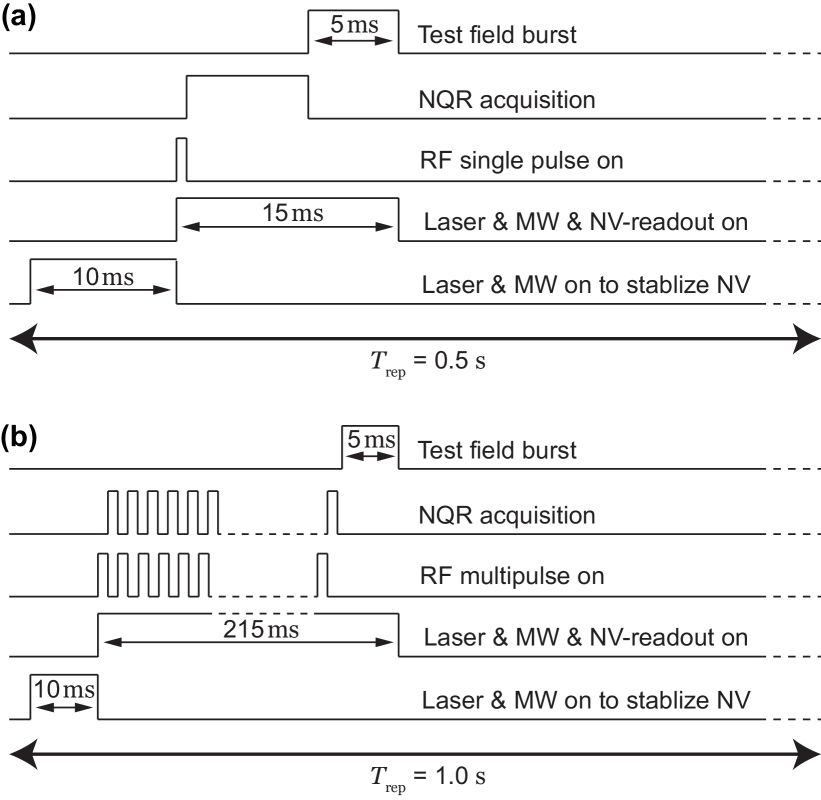
Figure A11: Timing protocol for NV NQR measurements. NV NQR measurement protocol used for (a) single-RF-pulse NQR experiments and (b) SLSE NQR experiments.

Appendix Appendix E

NQR setup

1 Timing diagram

Figure A11(a) shows the NV NQR measurement protocol used for the single-RF-pulse experiments (Figs. 4, 5 in the main text). To stabilize the NV fluorescence response, the laser and MW pulses are turned on for $10~{}{\rm ms}$ prior to acquiring NQR signals. Then, an RF excitation pulse is applied, and the synchronized XY8-20 NV signals are acquired for $15~{}{\rm ms}$. The MW and laser pulses are then turned off for the remaining $475~{}{\rm ms}$ of the sequence. We do this because we found that keeping the MW and laser pulses on for the entire repetition time, $T_{\rm rep}=500~{}{\rm ms}$, resulted in a broadening, shift, and eventual loss of the NQR signal after several minutes. This is likely due to a rise in temperature and temperature gradients across the NQR sample generated by heat dissipation from the laser and MW pulses. Fortunately, turning the pulses on for $25~{}{\rm ms}$ out of the total $500~{}{\rm ms}$ sequence time was a low enough duty cycle to eliminate this effect, while still allowing for acquisition of the full NQR transient signal.

A $100~{}{\rm pT_{rms}}$ RF test field with a frequency a-few-${\rm kHz}$ above the NQR frequency is applied for the last $5~{}{\rm ms}$ of the NV readout in each repetition, after the NQR signals had decayed. This “test-field burst” is added to monitor the magnetometer’s sensitivity over hours of averaging and make sure the NV test signal isn’t dropping below a threshold value. The test-field data were dropped when analyzing NQR signals. For NQR experiments with the the $4\mbox{-}\rm g$ sample (Fig. 5), the average NV test signal fluorescence was $V_{\rm nv}\approx 7~{}{\rm mV_{rms}}$, and the signal remained within a factor of $1.3$ of this level throughout the measurements. For NQR experiments with the $21\mbox{-}\rm g$ sample (Figs. 4 and 6), the average NV test signal fluorescence was $V_{\rm nv}\approx 6~{}{\rm mV_{rms}}$, and the signal remained within a factor of $1.15$ of this level throughout the measurements.

Figure A11(b) shows the NV NQR measurement protocol used for the RF multipulse SLSE experiment (Fig. 6 in the main text). The NV XY8-20 sequences are synchronized with the SLSE RF excitation pulses, and both pulse trains are applied for ${\sim}215~{}{\rm ms}$ in each repetition. In order to avoid heating of the sample, the repetition time in the SLSE experiment was set to be twice as long as in single-RF-pulse experiments, $T_{\rm rep}\,{=}\,1~{}{\rm s}$.

In order to alternate the phase of the RF excitation pulses, we combine the outputs of two Teledyne LeCroy waveform signal generators. The $10~{}{\rm MHz}$ frequency reference output of one generator is connected to the frequency reference input of the other to synchronize their internal clocks. The two RF sources are set to the same frequency and $90^{\degree}$ out of phase with each other. Each source is triggered by its own channel from the TTL pulse card; one trigger is repeated every $T_{\rm rep}=1~{}{\rm s}$ and the other is repeated every ${\sim}2~{}{\rm ms}$ (with an initial $1~{}{\rm ms}$ delay with respect to the first source), corresponding to the time delay between the echo pulses.

2 Sodium nitrite samples

Sodium nitrite (${\rm NaNO_{2}}$) powder sample was purchased from Sigma-Aldrich (Lot${\#}\,$MKBX1577V). Plastic cylinder containers with ${\sim}1~{}{\rm mm}$ wall thickness were assembled to hold the powder samples in the setup.

Table A3: Parameters of the RF coils used in the NQR experiments. The inductance was measured by an RLC-meter device. The quality factor, $Q$, was measured by the method discussed in 5.

Coil	Gauge	Turns	$\boldsymbol{D}$	$\boldsymbol{H}$	$\boldsymbol{V_{\rm c}}$	Inductance, $\boldsymbol{L}$	$\boldsymbol{Q}$
Small	21 AWG	20	23.1 mm	14.0 mm	5.9 ${\rm cm^{3}}$	8.3 ${\rm\upmu H}$	${\sim}8$
Big	20 AWG	58	21.6 mm	53.2 mm	19.5 ${\rm cm^{3}}$	23.5 ${\rm\upmu H}$	${\sim}23$

3 Thermal housing

To improve temperature stability during NQR measurements, a $0.5\mbox{-}{\rm inch}$-thick thermal insulation sheet was glued to the exterior walls of the aluminum-shield housing. A temperature control device (Thorlabs ITC4005) is used to control the temperature of a Peltier element which was thermally attached to the Al-shield with the help of silicone thermal paste.

4 RF pulse amplification

RF pulses are amplified by a 250-W RF power amplifier (Tomco BT00250-AlphaS) before entering a resonant multi-turn coil wrapped around the plastic cylinder container, see Fig. A12. In order to suppress the amplifier noise, two pairs of crossed-diodes with a minimum 100-V breakdown voltage (onsemi 1N4446) are connected in series to the amplifier’s output. Also, the amplifier is blanked before and after each RF pulse by applying a gated DC voltage to the amplifier’s TTL blanking port. From the fit in Fig. 4(c), the conversion factor between the applied RF pulse voltage to the amplifier and generated RF magnetic field amplitude inside the coil was found to be $K=B_{\rm rf}/V_{\rm rf}=5.01\pm 0.05~{}{\rm mT/V_{pp}}$.

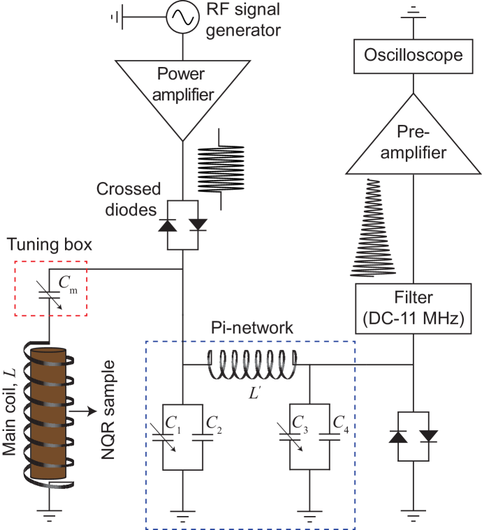
Figure A12: Block diagram of the setup used for NQR coil excitation and detection. $C_{\rm m}$, $C_{1}$, and $C_{3}$: variable ($9\mbox{-}200~{}{\rm pF}$) capacitors; $L$: inductance of the main coil (see Table A3); $C_{2}=0.9~{}{\rm nF}$, $C_{4}=0.22~{}{\rm nF}$, $L^{{}^{\prime}}\approx 1.7~{}{\rm\upmu H}$.

5 Resonant RF coil tuning circuit and pi-network

Parameters of the resonant RF coils wrapped around the sodium nitrite powder samples and used for exciting the $3.6~{}{\rm MHz}$ NQR transition are shown in Table A3. The small coil was used for the $4\mbox{-}\rm g$ sample (Fig. 5 in the main text) and the big coil was used for the $21\mbox{-}\rm g$ sample (Figs. 4 and 6 in the main text). Both coils were only partially filled with powder, so the coil volumes are larger than the actual sample volumes. A variable capacitor (Sprague-Goodman GZN20100) with capacitance $C_{\rm m}=9\mbox{-}200~{}{\rm pF}$ is connected in series with the RF coils (Fig. A12). For both RF coils, the combination of the variable capacitor and the coil’s parasitic capacitance provided the ability to tune the circuit to the $3.6~{}{\rm MHz}$ NQR transition. Adding the usual parallel tuning capacitor prevented us from tuning the circuit to $3.6~{}{\rm MHz}$, which implies that the self-resonance of each coil was already near $3.6~{}{\rm MHz}$. Even without the parallel tuning capacitor, the impedance matching was sufficient to excite and inductively detect NQR signals efficiently.

The same resonant RF coil is used for both exciting and detecting NQR signals. To do this, the signal voltage picked-up by the resonant RF coil is passed through a custom-built pi-network and a low-pass filter (MiniCircuits BLP-10.7), amplified by a low-noise pre-amplifier (NF CMP61665-2), and recorded by an oscilloscope.

The custom-built pi-network, Fig. A12 (dashed blue box), acts as a limiter that prevents the high-power RF excitation pulses from saturating the pre-amplifier, while still passing the weak inductive NQR signals Hiblot et al. (2008). A requirement is that the pi-network satisfies an “anti-resonance” condition $f_{0}\,{=}\,1/(2\pi\sqrt{L^{{}^{\prime}}(C_{1}+C_{2})})$, where $L^{{}^{\prime}}$, $C_{1}$, $C_{2}$ are pi-network elements defined in Fig. A12. Three pairs of crossed-diodes are inserted after the pi-network to complete the circuit. We tuned $C_{1}$ and $C_{3}$ to maximize the input impedance when the three diode pairs were shorted and minimize the reflection when there was no short.

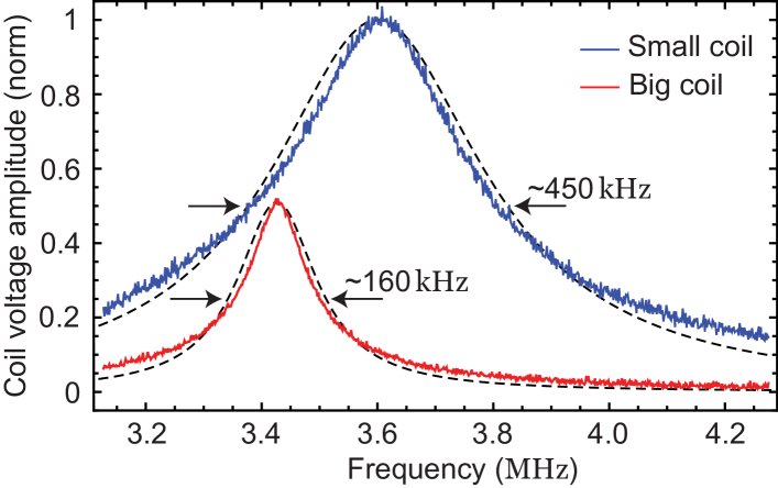
Figure A13: Coil quality factor. The loaded quality factor of the resonant RF coil was measured by sweeping the frequency of an RF signal applied to a single-turn loop and picking up the oscillating induced voltage by the resonant RF coil. Similar to Fig. A10(b), the amplitude of the oscillating voltage is extracted for each $1.66~{}{\rm kHz}$ segment, and plotted as a function of frequency for both resonant RF coils. The “Small coil” is the coil used for the 4-g sample, and the “Big coil” is the coil used for the 21-g sample. The spectra are fit to Lorentzian functions (dashed black lines) to extract the center frequency, $f_{0}$, and FWHM, $\Delta f$. The quality factor is estimated as $Q\,{=}\,f_{0}/\Delta f$ and is given in Table A3. Although the big coil’s resonance frequency is detuned from NQR resonance in this figure, it was always tuned to the $3.6~{}{\rm MHz}$ NQR frequency prior to performing NQR spectroscopy.

To characterize the resonant RF coil’s frequency response, a sinusoidal RF carrier was applied to a ${\sim}5.8~{}{\rm cm}$ diameter single-turn loop that was placed above the resonant RF coil. The carrier frequency was swept, and the oscillating induced voltage in the coil was recorded by the oscilloscope using the setup shown in Fig. A12. By adjusting the capacitance $C_{\rm m}$, the coil resonance frequency was tuned to the NQR frequency ($f_{0}=3.6~{}{\rm MHz}$). Figure A13 shows the amplitude of the induced voltage as a function of frequency for both coils. The amplitude was extracted from the oscillating signal using a similar procedure as described for Fig. A10(b). From these data, we estimate the loaded quality factor is $Q\approx 8$ for the small coil used for the 4-g sample and $Q\approx 23$ for the large coil used for the 21-g sample.

6 NQR Fourier transform spectra in the main text

For the NQR experiments, both the NV and coil readouts were synchronized by trigger pulses from the TTL pulse card. In Figs. 4(b,c,d) of the main text, the imaginary part of the Fourier transform of the time-domain NQR signals were taken because the symmetric lineshape of the spectra allowed us to determine the signals’ phases with sufficient precision. In Fig. 5(b) and Fig. 6(c) of the main text, the absolute value of the Fourier transform of the time-domain NQR signals were taken because the asymmetric lineshape prevented us from determining an exact phase.

Appendix Appendix F

Spin dynamics under NQR and RF excitation Hamiltonians

An NQR transition can be excited by applying a resonant RF magnetic field. In powder samples, an RF pulse applied along the $z$-axis (in the lab frame) can induce a magnetization oscillating at the NQR frequency, along the $z$-axis, given by:

$$M_{\rm z}^{\rm lab}~{}{=}~{}n_{\rm n}\,\gamma_{\rm n}\,h\,\langle I_{\rm z}^{\rm lab}\rangle,$$ (AVI-12)

where $n_{\rm n}$ is the nuclear-spin concentration in the sample, $\gamma_{\rm n}$ is the nuclear-spin gyromagnetic ratio, $h$ is the Planck constant, and $\langle I_{\rm z}^{\rm lab}\rangle$ is the expectation value of the nuclear-spin projection along the $z$-axis. In thermal equilibrium, the density operator populated under the nuclear quadrupole Hamiltonian $H_{\rm Q}$, Eq. (2), is:

$$\rho_{\rm 0}~{}{=}~{}\frac{e^{-hH_{\rm Q}/(k_{\rm B}T_{\rm s})}}{{\rm Tr}[e^{-hH_{\rm Q}/(k_{\rm B}T_{\rm s})}]},$$ (AVI-13)

where ${\rm Tr}$ is trace of the operator, $k_{\rm B}$ is the Boltzmann constant, and $T_{\rm s}$ is the sample temperature. In the high temperature approximation, Eq. (AVI-13) becomes:

$$\rho_{\rm 0}~{}{\approx}~{}\frac{\mathbbm{1}-hH_{\rm Q}/(k_{\rm B}T_{\rm s})}{2I+1},$$ (AVI-14)

where $\mathbbm{1}$ is the identity operator and $2I+1$ is the number of nuclear-spin energy levels.

The Hamiltonian describing the interaction of nuclear spins with an RF excitation field applied along the $z$-axis can be written (in frequency units) as:

$$\begin{split}H_{\rm rf}&(t)~{}{=}~{}-\gamma_{\rm n}B_{\rm rf}I_{\rm z}^{\rm lab}\cos{(2\pi\,f_{\rm rf}\,t)}\\ &\,~{}~{}~{}~{}{=}~{}-\gamma_{\rm n}B_{\rm rf}\cos{(2\pi\,f_{\rm rf}\,t)}\times\\ &~{}~{}~{}\bigl{[}I_{\rm x^{{}^{\prime}}}\sin{\theta}\cos{\varphi}+I_{\rm y^{{}^{\prime}}}\sin{\theta}\sin{\varphi}+I_{\rm z^{{}^{\prime}}}\cos{\theta}\bigr{]},\end{split}$$ (AVI-15)

where $B_{\rm rf}$ and $f_{\rm rf}$ are the amplitude and frequency of the RF magnetic field, respectively. In Eq. (AVI-15), $\{I_{\rm x^{{}^{\prime}}},I_{\rm y^{{}^{\prime}}},I_{\rm z^{{}^{\prime}}}\}$ are the unitless nuclear-spin operators along each principle axis of a given crystallite, $\theta$ is the polar angle and $\varphi$ is the azimuthal angle that the applied RF field vector makes with respect to the principle axes. For a spin-1 system ($I=1$, $\eta\,{\neq}\,0$), there are three NQR transitions with frequencies: $f_{\rm x^{{}^{\prime}}}=f_{\rm Q}(1\,{+}\,\eta/3)$ for the $E_{\rm z^{{}^{\prime}}}\leftrightarrow E_{\rm y^{{}^{\prime}}}$ transition, $f_{\rm y^{{}^{\prime}}}=f_{\rm Q}(1\,{-}\,\eta/3)$ for the $E_{\rm z^{{}^{\prime}}}\leftrightarrow E_{\rm x^{{}^{\prime}}}$ transition, and $f_{\rm z^{{}^{\prime}}}=2\,f_{\rm Q}\,\eta\,/3$ for the $E_{\rm x^{{}^{\prime}}}\leftrightarrow E_{\rm y^{{}^{\prime}}}$ transition, see Fig. 3(b). In the rotating frame of the quadrupolar Hamiltonian, the time-averaged RF Hamiltonian in resonance with one of the NQR transitions is reduced to:

$$\begin{split}\overline{\widehat{H}}_{\rm rf}~{}{=}~{}-\frac{\gamma_{\rm n}B_{\rm rf}}{2}&\times\\ &(I_{\rm x^{{}^{\prime}}}\sin{\theta}\cos{\varphi})~{}~{}{\rm if}~{}~{}f_{\rm rf}=f_{\rm x^{{}^{\prime}}}\\ &(I_{\rm y^{{}^{\prime}}}\sin{\theta}\sin{\varphi})~{}~{}{\rm if}~{}~{}f_{\rm rf}=f_{\rm y^{{}^{\prime}}}\\ &(I_{\rm z^{{}^{\prime}}}\cos{\theta})~{}~{}~{}~{}~{}~{}~{}~{}\,{\rm if}~{}~{}f_{\rm rf}=f_{\rm z^{{}^{\prime}}}.\end{split}$$ (AVI-16)

The density operator’s time evolution can be described by the Liouville equation. Following an RF-excitation pulse of length $t_{\rm rf}$, the density operator in the rotating frame becomes:

$$\hat{\rho_{1}}~{}{=}~{}e^{-i\,2\pi\overline{\widehat{H}}_{\rm rf}t_{\rm rf}}\hat{\rho_{\rm 0}}e^{i\,2\pi\overline{\widehat{H}}_{\rm rf}t_{\rm rf}}.$$ (AVI-17)

An RF excitation pulse applied at the $f_{\rm y^{{}^{\prime}}}$ resonance frequency induces an oscillating magnetization along the $y^{\prime}$-axis of each crystallite. The expectation value of the spin projection along the $z$-axis is:

$$\begin{split}\langle I_{\rm z}^{\rm lab}(t_{0},\alpha)\rangle~{}{=}~{}&{\rm Tr}[I_{\rm z}^{\rm lab}e^{-i\,2\pi H_{\rm Q}t_{0}}\hat{\rho_{1}}e^{i2\pi H_{\rm Q}t_{0}}]\\ {=}~{}&{\rm Tr}[(I_{\rm y^{{}^{\prime}}}\sin{\theta}\sin{\varphi})e^{-i2\pi H_{\rm Q}t_{0}}\hat{\rho_{1}}e^{i2\pi H_{\rm Q}t_{0}}]\\ {=}~{}\frac{h\,f_{\rm y^{{}^{\prime}}}}{3\,k_{\rm B}\,T_{\rm s}}&\sin{(2\pi f_{\rm y^{{}^{\prime}}}t_{0})}\sin{(\alpha\sin{\theta}\sin{\varphi})}\sin{\theta}\sin{\varphi}.\end{split}$$ (AVI-18)

In Eq. (AVI-18), $t_{0}$ is the time after the RF pulse and $\alpha=2\pi\gamma_{\rm n}B_{\rm rf}t_{\rm rf}$ is the RF nutation angle in radians. Inserting Eq. (AVI-18) into Eq. (AVI-12) and averaging over all $\theta$ and $\varphi$ to take the limit of many randomly-oriented crystallites, the net NQR magnetization in the lab frame becomes:

$$\begin{split}M_{\rm z}^{\rm lab}({t_{0},\alpha})&~{}{=}~{}n_{\rm n}\,\gamma_{\rm n}\,\frac{h^{2}f_{\rm y^{{}^{\prime}}}}{3\,k_{\rm B}\,T_{\rm s}}\sin{(2\pi f_{\rm y^{{}^{\prime}}}t_{0})}\times\\ \int_{0}^{\pi}\int_{0}^{2\pi}&\frac{1}{4\pi}\biggl{[}\sin{(\alpha\sin{\theta}\sin{\varphi})}\sin{\theta}\sin{\varphi}\biggr{]}\sin{\theta}\,d\theta\,d\varphi\\ ~{}{=}~{}&n_{\rm n}\,\gamma_{\rm n}\,\frac{h^{2}f_{\rm y^{{}^{\prime}}}}{3\,k_{\rm B}\,T_{\rm s}}\sin{(2\pi f_{\rm y^{{}^{\prime}}}t_{0})}\sqrt{\frac{\pi}{2\alpha}}\,J_{3/2}(\alpha),\end{split}$$ (AVI-19)

where $J_{3/2}$ is the Bessel function of first kind and order 3/2. In Eq. (AVI-19), the nutation function, $\sqrt{\pi/(2\alpha)}\,J_{3/2}(\alpha)$, has a maximum of ${\sim}0.436$ for an RF excitation pulse with $\alpha\,{\approx}\,2.08\,{\rm rad}\,{=}\,119^{\degree}$. Therefore, the amplitude of the NQR magnetization immediately after an optimal RF excitation pulse can be written as Garroway et al. (2001):

$$M_{\rm z}^{\rm lab}~{}{\approx}~{}0.436\,n_{\rm n}\,\gamma_{\rm n}\,\frac{h^{2}f_{\rm y^{{}^{\prime}}}}{3\,k_{\rm B}\,T_{\rm s}}.$$ (AVI-20)

Using the same steps as above, it can be shown that in the case of a powder, the NQR magnetization components on a plane perpendicular to the RF field direction average to zero, i.e. $M_{\rm x}^{\rm lab}=M_{\rm y}^{\rm lab}=0$. Using Eq. AVI-20 and for the case of ${}^{14}{\rm N}$ nuclear spins in a perfectly packed sodium nitrite powder at room temperature ($n_{\rm n}\,{=}\,1.89\times 10^{22}~{}{\rm cm^{-3}}$, $\gamma_{\rm n}\,{=}\,3.077~{}{\rm MHz/T}$, $f_{\rm y^{{}^{\prime}}}\,{=}\,3.608~{}{\rm MHz}$, $T_{\rm s}\,{=}\,293~{}{\rm K}$), the nuclear-spin projection induced by an optimal RF pulse is calculated to be $\langle I_{\rm z}^{\rm lab}\rangle\,{=}\,8.6\times 10^{-8}$ which results in an NQR magnetization $M_{\rm z}^{\rm lab}\,{=}\,M_{0}\,{=}\,3.3~{}{\rm\upmu A/m}$ in the sample.

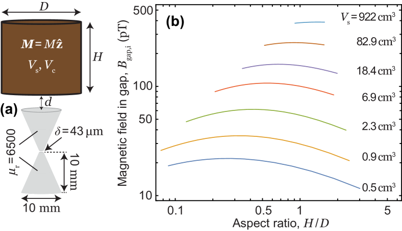
Figure A14: Magnetic field in the gap vs sample aspect ratio. (a) Diagram of the model used for the finite-element simulations. The sample was modeled as a cylindrical magnet with height $H$, diameter $D$, and a uniform magnetization $M$ along the $z$-axis. The distance from the bottom of the sample to the top of the cones is $d$. Two ferrite cones with relative permeability $\mu_{\rm r}\,{=}\,6500$, $10~{}{\rm mm}$ length, $10~{}{\rm mm}$ base diameter, and $370~{}{\rm\upmu m}$ truncated-tip-diameter are arranged in a bowtie configuration with the gap length ${\delta}\,{=}\,43~{}{\rm\upmu m}$. (b) Average magnetic field within the gap calculated as a function of the cylinder’s aspect ratio $H/D$ for different sample volumes $V_{\rm s}$. Here, $d\,{=}\,4~{}{\rm mm}$ and the sample magnetization was set to $M\,{=}\,M_{0}\,{=}\,3.3~{}{\rm\upmu A/m}$.

Appendix Appendix G

Simulation of ferrite cones and a magnetized cylinder

Figure A14(a) describes the model we used for the initial finite-element simulations presented in Fig. 3(c) in the main text. The sample was modeled as a cylindrical magnet, with volume $V_{\rm s}$ and uniform magnetization $M\,{=}\,M_{0}\,{=}\,3.3~{}{\rm\upmu A/m}$ along the $z$-axis, located a distance $d=4~{}{\rm mm}$ above the cones. Figure A14(b) shows the initial nuclear AC magnetic field amplitude in the gap, $B_{\rm gap,i}$, calculated for different sample volumes and aspect ratios. As $V_{s}$ increases, the optimal aspect ratio shifts to larger values and the peak value of $B_{\rm gap,i}$ increases. However, for $V_{\rm s}\,{\gtrsim}\,100~{}{\rm cm^{3}}$, $B_{\rm gap,i}$ begins to saturate to a practically-achievable maximum value of ${\sim}500~{}{\rm pT}$. The peak value of $B_{\rm gap,i}$ for each value of $V_{s}$ were plotted in Fig. 3(c) in the main text.

Several parameters in the experiment turned out to be different from the optimal geometry we initially modeled for. Taking into account the sodium nitrite powder filling fraction inside the coils (Table A3) and the magnetization amplification due to the resonant RF coil, Eq. (3), the effective NQR magnetization for the $4\mbox{-}\rm g$ and $21\mbox{-}\rm g$ samples are estimated to be $M_{\rm eff}\,{\approx}\,8~{}{\rm\upmu A/m}$ and $M_{\rm eff}\,{\approx}\,37~{}{\rm\upmu A/m}$, respectively. Also, instead of the $d=4~{}{\rm mm}$ standoff we initially assumed in the model, the standoffs from the bottom of the coils to the top of the cones were measured to be ${\sim}\,5~{}{\rm mm}$ in the $4\mbox{-}\rm g$ NQR experiment and ${\sim}\,9~{}{\rm mm}$ in the $21\mbox{-}\rm g$ experiment. Finally, the gap length was corrected to $\delta\,{=}\,40~{}{\rm\upmu m}$ (due to a small glue layer), which resulted in a simulated DC enhancement of $\epsilon\,{=}\,300$.

Using these experimental conditions, we carried out new simulations for the 4-g and 21-g samples. The “samples”, in this case, had the dimensions of the respective coils (Tab. A3), and the magnetization was set as the calculated values of $M_{\rm eff}$. After these adjustments, the calculated initial magnetic field amplitude in the gap was $B_{\rm gap,i}\,{\approx}\,230~{}{\rm pT}$ for the 4-g sample and $B_{\rm gap,i}\,{\approx}\,930~{}{\rm pT}$ for the 21-g sample. Converting these values to equivalent uniform magnetic fields ($B_{\rm equiv,i}\,{=}\,B_{\rm gap,i}/\epsilon$ with $\epsilon\,{=}\,300$) gives $B_{\rm equiv,i}\,{\approx}\,760~{}{\rm fT}$ for the $4\mbox{-}\rm g$ sample and $B_{\rm equiv,i}\,{\approx}\,3100~{}{\rm fT}$ for the $21\mbox{-}\rm g$ sample. These estimates were much closer to the experimentally observed values, well within a factor of 2.

Appendix Appendix H

Signal-to-noise ratio improvement in SLSE

In the SLSE experiments, the NQR signals following the echo pulses decay exponentially with an effective relaxation time $T_{\rm 2}^{\rm SLSE}$. $T_{\rm 2}^{\rm SLSE}$ is typically much longer than the decay of an NQR transient following a single RF pulse, and it is typically limited only by homonuclear dipolar and spin-lattice couplings in the sample Gregorovič and Apih (2008). For this reason, SLSE is often applied to increase the SNR of NQR spectra.

In order to find the NQR SNR for each acquisition time in the SLSE experiment, shown in Fig. 6(e), the first-25 NV readouts with ${\sim}1.65~{}{\rm ms}$ length were averaged together in the time-domain. A digital high-pass filter with cutoff frequency $2.6~{}{\rm kHz}$ and a Tukey window function centered to the middle of the time-averaged data were applied. Then, the absolute value of the Fourier transform was taken to obtain the NQR spectrum for each echo burst. The SLSE SNR was found by dividing the signal level (contained within a single frequency point, see Fig. 6) by the average noise within the $9{-}12~{}{\rm kHz}$ alias-frequency band. The noise floor in the SLSE experiment was found to be ${\sim}160~{}{\rm fT_{rms}\,s^{1/2}}$.

To find the SNR in the single-RF-pulse experiments, the initial ${\sim}3.85~{}{\rm ms}$ of the NV readout obtained at $21.8\,{\rm{}^{\circ}C}$ temperature (green spectrum in Fig. 4(d)) was selected. A Lorentz-to-Gauss window function $W(t)\,{=}\,\exp(0.085\,t)\exp(-(0.04\,t)^{2})$ was applied, and the absolute value of the Fourier transform was taken to obtain an NQR spectrum. The SNR was found by dividing the signal level to the average noise within the $8{-}11~{}{\rm kHz}$ alias-frequency band. The noise floor in the single-RF-pulse experiment was found to be ${\sim}400~{}{\rm fT_{rms}\,s^{1/2}}$.

In Fig. 6(b), the SLSE signal amplitude for the $21\mbox{-}\rm g$ sample is $B_{\rm equiv,i}\approx 0.5~{}{\rm pT}$, which is ${\sim}3$-times less than the one obtained in the single-RF-pulse experiments (Fig. 4(a), bottom). This can be due to variation in sample temperature and thermal gradients which led to a detuning of the RF pulses and reduced their fidelity Malone et al. (2011). Nevertheless, for a given experimental acquisition time, we found that the SLSE SNR exhibits a ${\sim}3$-fold improvement over the SNR in the single-RF-pulse experiments, see Fig. 6(e). This improvement is due to an order-of-magnitude higher measurement duty cycle and the ${\sim}2.5$-times lower noise floor in the SLSE experiment. The latter effect was not expected but may have been due to RF interference being worse during the single-RF-pulse experiment.

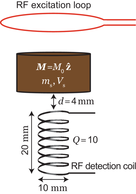
Figure A15: Remote NQR detection. Schematic of a setup for remotely-detected NQR spectroscopy. The sample has mass $m_{\rm s}$, volume $V_{\rm s}$, and magnetization $M_{0}$. The NQR transition is excited by a non-resonant wire loop located far enough from the sample to neglect resonant signal amplification. The detection coil has a loaded quality factor $Q\,{=}\,10$ and volume $V_{\rm c}=1.5~{}{\rm cm^{3}}$ (similar to the volume of our ferrite-cones-diamond magnetometer).

Appendix Appendix I

Calculations of resonant-induction amplification

1 Johnson-noise-limited SNR with a resonant-RF-coil and comparison to experiment

In Sec. V of the main text, we calculated the Johnson-noise-limited SNR (${\rm SNR_{J}}$) of NQR detection for the case when a resonant RF coil is used for signal amplification. Note that Eq. (5) neglects any deadtimes due to re-thermalization, so it is valid only for the interval of a measurement where the NQR signal is large. Realistically, for a single-RF-pulse experiment where the signal is averaged over many repetitions, the SNR would be a factor of ${\sim}(T_{\rm 1,nuc}/T_{\rm 2,nuc}^{\ast})^{1/2}$ lower than in Eq. (5). Note also that in Eq. (4) of the main text, the Johnson noise was derived using magnetic units of ${\rm T_{rms}}$. In order to derive the Johnson-noise-limited SNR, Eq. (5), we converted the Johnson noise to magnetic amplitude units ($\rm T$) by multiplying by $\sqrt{2}$.

We also estimated that ${\rm SNR_{J}}$ is ${\sim}2$ orders of magnitude higher than the NQR SNR in our ferrite-cones diamond RF magnetometer. This assumes that the diamond RF magnetometer’s sensitivity is ${\sim}200~{}{\rm fT_{rms}\,s^{1/2}}$, see Fig. 2(e), and that the signal amplitudes are $500~{}{\rm fT}$ for the 4-g sample and $2300~{}{\rm fT}$ for the 21-g sample, see Fig. 3(c). Here we neglect a possible factor of $\sqrt{2}$ that comes from converting noise in units of $\rm T\,s^{1/2}$ to $\rm T\,Hz^{-1/2}$ Fescenko et al. (2020).

2 Johnson magnetic noise in our experiment

It is worthwhile to directly calculate the effect of the resonant RF coil’s Johnson noise on the diamond RF magnetometer to verify it was not limiting our sensitivity. Using Eq. (4) and parameters of our RF coil assemblies (Table A3), the rms Johnson magnetic noise inside the resonant RF coils at room temperature is calculated to be $\eta_{\rm J}\approx 35~{}{\rm fT_{rms}\,Hz^{-1/2}}$ for the small coil and $\eta_{\rm J}\approx 32~{}{\rm fT_{rms}\,Hz^{-1/2}}$ for the big coil. However, our diamond RF magnetometer is located outside of the coil in a remote-detection configuration. In remotely-detected NQR, the magnetic field produced by the sample decays with increasing standoff, resulting in a loss of signal amplitude. The loss factor can be defined as $\alpha_{\rm loss}=B_{\rm equiv,i}/(\mu_{0}M_{\rm eff})$. Based on the calculations in Appendix G, we estimate $\alpha_{\rm loss}\approx 0.08$ for the $4\mbox{-}\rm g$ NQR experiment and $\alpha_{\rm loss}\approx 0.07$ for the $21\mbox{-}\rm g$ experiment. Using these factors, the equivalent Johnson noise that would be detected by our diamond RF magnetometer is ${\sim}2.8~{}{\rm fT_{\rm rms}\,Hz^{-1/2}}$ for the small coil and ${\sim}2.2~{}{\rm fT_{\rm rms}\,Hz^{-1/2}}$ for the big coil. These noise levels are much lower than the photoelectron-shot-noise-limited sensitivity of our diamond RF magnetometer and thus are negligible in the present experiments.

3 Remote NQR detection

The remote-detected NQR sensitivity calculations presented in Sec. V of the main text assumed the geometry depicted in Fig. A15. A non-resonant single-turn loop far from a sodium nitrite powder sample is used to excite its $3.6~{}{\rm MHz}$ NQR transition. The equivalent sensitivity of a Johnson-noise-limited RF coil to external magnetic fields is $\eta_{\rm J}/Q$, where $\eta_{\rm J}$ is given in Eq. (4). The factor of $1/Q$ comes because any external fields would be amplified by a factor of ${\sim}Q$ due to resonant induction. For an RF coil with volume $V_{\rm c}=1.5~{}{\rm cm^{3}}$ (equivalent to our ferrite-cones diamond RF magnetometer volume) and loaded quality factor $Q=10$, the sensitivity is calculated to be $\eta_{\rm J}/Q\,{\approx}\,8~{}{\rm fT_{rms}\,Hz^{-1/2}}$. This sensitivity is ${\sim}9$ times better than our ferrite-cones diamond magnetometer’s sensitivity if we assume the measured sensitivity of ${\sim}70~{}{\rm fT_{rms}\,s^{1/2}}$ at $0.35~{}{\rm MHz}$.

References

- Barry et al. (2020) J. F. Barry, J. M. Schloss, E. Bauch, M. J. Turner, C. A. Hart, L. M. Pham, and R. L. Walsworth, “Sensitivity optimization for NV-diamond magnetometry,” Reviews of Modern Physics 92, 15004 (2020).
- Barry et al. (2016) J. F. Barry, M. J. Turner, J. M. Schloss, D. R. Glenn, Y. Song, M. D. Lukin, H. Park, and R. L. Walsworth, “Optical magnetic detection of single-neuron action potentials using quantum defects in diamond,” Proceedings of the National Academy of Sciences of the United States of America 113, 14133 (2016).
- Fescenko et al. (2020) I. Fescenko, A. Jarmola, I. Savukov, P. Kehayias, J. Smits, J. Damron, N. Ristoff, N. Mosavian, and V. M. Acosta, “Diamond magnetometer enhanced by ferrite flux concentrators,” Physical Review Research 2, 23394 (2020).
- Eisenach et al. (2021) E. R. Eisenach, J. F. Barry, M. F. O’Keeffe, J. M. Schloss, M. H. Steinecker, D. R. Englund, and D. A. Braje, “Cavity-enhanced microwave readout of a solid-state spin sensor,” Nature Communications 12, 1 (2021).
- Zhang et al. (2021) C. Zhang, F. Shagieva, M. Widmann, M. Kübler, V. Vorobyov, P. Kapitanova, E. Nenasheva, R. Corkill, O. Rhrle, K. Nakamura, H. Sumiya, S. Onoda, J. Isoya, and J. Wrachtrup, “Diamond Magnetometry and Gradiometry towards Subpicotesla dc Field Measurement,” Physical Review Applied 15, 1 (2021).
- Masuyama et al. (2018) Y. Masuyama, K. Mizuno, H. Ozawa, H. Ishiwata, Y. Hatano, T. Ohshima, T. Iwasaki, and M. Hatano, “Extending coherence time of macro-scale diamond magnetometer by dynamical decoupling with coplanar waveguide resonator,” Review of Scientific Instruments 89, 125007 (2018).
- Glenn et al. (2018) D. R. Glenn, D. B. Bucher, J. Lee, M. D. Lukin, H. Park, and R. L. Walsworth, “High-resolution magnetic resonance spectroscopy using a Solid-State spin sensor,” Nature 555, 351 (2018).
- Smits et al. (2019) J. Smits, J. T. Damron, P. Kehayias, A. F. McDowell, N. Mosavian, I. Fescenko, N. Ristoff, A. Laraoui, A. Jarmola, and V. M. Acosta, “Two-dimensional nuclear magnetic resonance spectroscopy with a microfluidic diamond quantum sensor,” Science Advances 5, eaaw7895 (2019).
- Wang et al. (2022) Z. Wang, F. Kong, P. Zhao, Z. Huang, P. Yu, Y. Wang, F. Shi, and J. Du, “Picotesla magnetometry of microwave fields with diamond sensors,” Science Advances 8 (2022).
- Alsid et al. (2022) S. T. Alsid, J. M. Schloss, M. H. Steinecker, J. F. Barry, A. C. Maccabe, G. Wang, P. Cappellaro, and D. A. Braje, “A Solid-State Microwave Magnetometer with Picotesla-Level Sensitivity,” arXiv:2206.15440 (2022).
- Savukov et al. (2005) I. M. Savukov, S. J. Seltzer, M. V. Romalis, and K. L. Sauer, “Tunable atomic magnetometer for detection of radio-frequency magnetic fields,” Physical Review Letters 95, 3 (2005).
- Ledbetter et al. (2007) M. P. Ledbetter, V. M. Acosta, S. M. Rochester, D. Budker, S. Pustelny, and V. V. Yashchuk, “Detection of radio-frequency magnetic fields using nonlinear magneto-optical rotation,” Physical Review A 75, 023405 (2007).
- Griffith et al. (2010) W. C. Griffith, S. Knappe, and J. Kitching, “Femtotesla atomic magnetometry in a microfabricated vapor cell,” Optics Express 18, 27167 (2010).
- Wasilewski et al. (2010) W. Wasilewski, K. Jensen, H. Krauter, J. J. Renema, M. V. Balabas, and E. S. Polzik, “Quantum Noise Limited and Entanglement-Assisted Magnetometry,” Physical Review Letters 104, 133601 (2010).
- Dhombridge et al. (2022) J. E. Dhombridge, N. R. Claussen, J. Iivanainen, and P. D. D. Schwindt, “High-Sensitivity rf Detection Using an Optically Pumped Comagnetometer Based on Natural-Abundance Rubidium with Active Ambient-Field Cancellation,” Physical Review Applied 10, 1 (2022).
- Chalupczak et al. (2012) W. Chalupczak, R. M. Godun, S. Pustelny, and W. Gawlik, “Room temperature femtotesla radio-frequency atomic magnetometer,” Applied Physics Letters 100, 242401 (2012).
- Keder et al. (2014) D. A. Keder, D. W. Prescott, A. W. Conovaloff, and K. L. Sauer, “An unshielded radio-frequency atomic magnetometer with sub-femtoTesla sensitivity,” AIP Advances 4, 127159 (2014).
- Clarke (1980) J. Clarke, “Advances in SQUID Magnetometers,” IEEE Transactions on Electron Devices 27, 1896 (1980).
- Schmelz et al. (2016) M. Schmelz, V. Zakosarenko, A. Chwala, T. Schönau, R. Stolz, S. Anders, S. Linzen, and H. G. Meyer, “Thin-Film-Based Ultralow Noise SQUID Magnetometer,” IEEE Transactions on Applied Superconductivity 26, 1 (2016).
- Storm et al. (2017) J.-H. Storm, P. Hömmen, D. Drung, and R. Körber, “An ultra-sensitive and wideband magnetometer based on a superconducting quantum interference device,” Applied Physics Letters 110, 072603 (2017).
- Li et al. (2021) Z.-H. Li, T.-Y. Wang, Q. Guo, H. Guo, H.-F. Wen, J. Tang, and J. Liu, “Enhancement of magnetic detection by ensemble NV color center based on magnetic flux concentration effect,” Acta Physica Sinica 70, 147601 (2021).
- Xie et al. (2022) Y. Xie, C. Xie, Y. Zhu, K. Jing, Y. Tong, X. Qin, H. Guan, C.-K. Duan, Y. Wang, X. Rong, and J. Du, “-limited dc Quantum Magnetometry via Flux Modulation,” arXiv:2204.07343 (2022).
- Taylor et al. (2008) J. M. Taylor, P. Cappellaro, L. Childress, L. Jiang, D. Budker, P. R. Hemmer, A. Yacoby, R. Walsworth, and M. D. Lukin, “High-sensitivity diamond magnetometer with nanoscale resolution,” Nature Physics 4, 810 (2008).
- Connor et al. (1990) C. Connor, J. Chang, and A. Pines, “Magnetic resonance spectrometer with a dc SQUID detector,” Review of Scientific Instruments 61, 1059 (1990).
- Augustine et al. (1998) M. P. Augustine, D. M. TonThat, and J. Clarke, “SQUID detected NMR and NQR,” Solid State Nuclear Magnetic Resonance 11, 139 (1998).
- Lee et al. (2006) S. K. Lee, K. L. Sauer, S. J. Seltzer, O. Alem, and M. V. Romalis, “Subfemtotesla radio-frequency atomic magnetometer for detection of nuclear quadrupole resonance,” Applied Physics Letters 89, 23 (2006).
- Das and Hahn (1958) T. Das and E. Hahn, Nuclear quadrupole resonance spectroscopy (Academic Press, 1958).
- Zax et al. (1985) D. B. Zax, A. Bielecki, K. W. Zilm, A. Pines, and D. P. Weitekamp, “Zero field NMR and NQR,” The Journal of Chemical Physics 83, 4877 (1985).
- Garroway et al. (2001) A. N. Garroway, M. L. Buess, J. B. Miller, B. H. Suits, A. D. Hibbs, G. A. Barrall, R. Matthews, and L. J. Burnett, “Remote sensing by nuclear quadrupole resonance,” IEEE Transactions on Geoscience and Remote Sensing 39, 1108 (2001).
- Kim et al. (2014) Y. J. Kim, T. Karaulanov, A. N. Matlashov, S. Newman, A. Urbaitis, P. Volegov, J. Yoder, and M. A. Espy, “Polarization enhancement technique for nuclear quadrupole resonance detection,” Solid State Nuclear Magnetic Resonance 61-62, 35 (2014).
- Malone et al. (2020) M. W. Malone, M. A. Espy, S. He, M. T. Janicke, and R. F. Williams, “The 1H T1 dispersion curve of fentanyl citrate to identify NQR parameters,” Solid State Nuclear Magnetic Resonance 110, 101697 (2020).
- Balchin et al. (2005) E. Balchin, D. J. Malcolme-Lawes, I. J. Poplett, M. D. Rowe, J. A. Smith, G. E. Pearce, and S. A. Wren, “Potential of nuclear quadrupole resonance in pharmaceutical analysis,” Analytical Chemistry 77, 3925 (2005).
- Lužnik et al. (2013) J. Lužnik, J. Pirnat, V. Jazbinšek, Z. Lavrič, S. Srčič, and Z. Trontelj, “The Influence of Pressure in Paracetamol Tablet Compaction on 14N Nuclear Quadrupole Resonance Signal,” Applied Magnetic Resonance 44, 735 (2013).
- Kyriakidou et al. (2015) G. Kyriakidou, A. Jakobsson, K. Althoefer, and J. Barras, “Batch-Specific Discrimination Using Nuclear Quadrupole Resonance Spectroscopy,” Analytical Chemistry 87, 3806 (2015).
- Lyfar et al. (1976) D. L. Lyfar, V. E. Goncharuk, and S. M. Ryabchenko, “Temperature Dependence of Nuclear Quadrupole Resonance in Layer-Type Crystals,” physica status solidi (b) 76, 183 (1976).
- Sharma et al. (1986) S. Sharma, H. Paulus, N. Weiden, and A. Weiss, “Crystal Structure and Single Crystal 35 Cl NQR of 1,2-Dichloro-3-Nitrobenzene, Cl (1) Cl (2) (NO 2 ) (3) C 6 H 3,” Zeitschrift für Naturforschung A 41, 134 (1986).
- Horiuchi et al. (1990) K. Horiuchi, T. Shimizu, H. Iwafune, T. Asaji, and D. Nakamura, “Temperature Dependences of NQR Frequencies and Nuclear Quadrupole Relaxation Times of Chlorine in 2, 6-Lutidinium Hexachlorotellurate(IV) as Studied by Pulsed NQR Techniques,” Zeitschrift fur Naturforschung - Section A Journal of Physical Sciences 45, 485 (1990).
- Huebner et al. (1999) M. Huebner, J. Leib, and G. Eska, “NQR on Gallium Single Crystals for Absolute Thermometry at Very Low Temperatures,” Journal of Low Temperature Physics 114, 203 (1999).
- Lang et al. (2010) G. Lang, H. J. Grafe, D. Paar, F. Hammerath, K. Manthey, G. Behr, J. Werner, and B. Büchner, “Nanoscale electronic order in iron pnictides,” Physical Review Letters 104, 3 (2010).
- Malone et al. (2016) M. W. Malone, G. A. Barrall, M. A. Espy, M. C. Monti, D. A. Alexson, and J. K. Okamitsu, “Polarization enhanced Nuclear Quadrupole Resonance with an atomic magnetometer,” in Detection and Sensing of Mines, Explosive Objects, and Obscured Targets XXI, Vol. 9823, edited by S. S. Bishop and J. C. Isaacs (2016) p. 98230Z.
- Lovchinsky et al. (2017) I. Lovchinsky, J. D. Sanchez-Yamagishi, E. K. Urbach, S. Choi, S. Fang, T. I. Andersen, K. Watanabe, T. Taniguchi, A. Bylinskii, E. Kaxiras, P. Kim, H. Park, and M. D. Lukin, “Magnetic resonance spectroscopy of an atomically thin material using a single-spin qubit,” Science 355, 503 (2017).
- Henshaw et al. (2022) J. Henshaw, P. Kehayias, M. Saleh Ziabari, M. Titze, E. Morissette, K. Watanabe, T. Taniguchi, J. I. A. Li, V. M. Acosta, E. S. Bielejec, M. P. Lilly, and A. M. Mounce, “Nanoscale solid-state nuclear quadrupole resonance spectroscopy using depth-optimized nitrogen-vacancy ensembles in diamond,” Applied Physics Letters 120, 174002 (2022).
- Shin et al. (2014) C. S. Shin, M. C. Butler, H. J. Wang, C. E. Avalos, S. J. Seltzer, R. B. Liu, A. Pines, and V. S. Bajaj, “Optically detected nuclear quadrupolar interaction of N 14 in nitrogen-vacancy centers in diamond,” Physical Review B - Condensed Matter and Materials Physics 89, 1 (2014).
- Oja et al. (1967) T. Oja, R. A. Marino, and P. J. Bray, “14N nuclear quadrupole resonance in the ferroelectric phase of sodium nitrite,” Physics Letters A 26, 11 (1967).
- Petersen and Bray (1976) G. Petersen and P. J. Bray, “14N nuclear quadrupole resonance and relaxation measurements of sodium nitrite,” The Journal of Chemical Physics 64, 522 (1976).
- National Magnetics Group-Inc. (2019) National Magnetics Group-Inc., “High Permeability Mn-Zn Ferrite,” (2019).
- Bolton (2016) T. Bolton, Optimal design of electrically-small loop antenna including surrounding medium effects, Ph.D. thesis (2016).
- Fisher et al. (1999) G. Fisher, E. MacNamara, R. E. Santini, and D. Raftery, “A versatile computer-controlled pulsed nuclear quadrupole resonance spectrometer,” Review of Scientific Instruments 70, 4676 (1999).
- Hiblot et al. (2008) N. Hiblot, B. Cordier, M. Ferrari, A. Retournard, D. Grandclaude, J. Bedet, S. Leclerc, and D. Canet, “A fully homemade 14N quadrupole resonance spectrometer,” Comptes Rendus Chimie 11, 568 (2008).
- Vega (1974) S. Vega, “Theory of T1 relaxation measurements in pure nuclear quadrupole resonance for spins I = 1,” The Journal of Chemical Physics 61, 1093 (1974).
- Suits (2006) B. H. Suits, “NUCLEAR QUADRUPOLE RESONANCE SPECTROSCOPY,” in Handbook of Applied Solid State Spectroscopy, edited by D. R. Vij (Springer US, Boston, MA, 2006) pp. 65–96.
- Bloom et al. (1955) M. Bloom, E. L. Hahn, and B. Herzog, “Free magnetic induction in nuclear quadrupole resonance,” Physical Review 97, 1699 (1955).
- Qiu et al. (2007) L. Qiu, Y. Zhang, H.-J. Krause, A. I. Braginski, and A. Usoskin, “High-temperature superconducting quantum interference device with cooled LC resonant circuit for measuring alternating magnetic fields with improved signal-to-noise ratio,” Review of Scientific Instruments 78, 054701 (2007).
- Greer et al. (2021) M. Greer, D. Ariando, M. Hurlimann, Y. Q. Song, and S. Mandal, “Analytical models of probe dynamics effects on NMR measurements,” Journal of Magnetic Resonance 327, 106975 (2021).
- Verber et al. (1962) C. M. Verber, H. P. Mahon, and W. H. Tanttila, “Nuclear Resonance of Aluminum in Synthetic Ruby,” Physical Review 125, 1149 (1962).
- Marino and Klainer (1977) R. A. Marino and S. M. Klainer, “Multiple spin echoes in pure quadrupole resonance,” The Journal of Chemical Physics 67, 3388 (1977).
- Cantor and Waugh (1980) R. S. Cantor and J. S. Waugh, “Pulsed spin locking in pure nuclear quadrupole resonance,” The Journal of Chemical Physics 73, 1054 (1980).
- Maricq (1986) M. M. Maricq, “Quasistationary state and its decay to equilibrium in the pulsed spin locking of a nuclear quadrupole resonance,” Physical Review B 33, 4501 (1986).
- Malone et al. (2011) M. W. Malone, M. McGillvray, and K. L. Sauer, “Revealing dipolar coupling with NQR off-resonant pulsed spin locking,” Physical Review B - Condensed Matter and Materials Physics 84, 1 (2011).
- Clevenson et al. (2015) H. Clevenson, M. E. Trusheim, C. Teale, T. Schröder, D. Braje, and D. Englund, “Broadband magnetometry and temperature sensing with a light-trapping diamond waveguide,” Nature Physics 11, 393 (2015).
- Xu et al. (2019) L. Xu, H. Yuan, N. Zhang, J. Zhang, G. Bian, P. Fan, M. Li, C. Zhang, Y. Zhai, and J. Fang, “High-efficiency fluorescence collection for NV- center ensembles in diamond,” Opt. Express 27, 10787 (2019).
- Le Sage et al. (2012) D. Le Sage, L. M. Pham, N. Bar-Gill, C. Belthangady, M. D. Lukin, A. Yacoby, and R. L. Walsworth, “Efficient photon detection from color centers in a diamond optical waveguide,” Phys. Rev. B 85, 121202 (2012).
- Zhou et al. (2020) H. Zhou, J. Choi, S. Choi, R. Landig, A. M. Douglas, J. Isoya, F. Jelezko, S. Onoda, H. Sumiya, P. Cappellaro, H. S. Knowles, H. Park, and M. D. Lukin, “Quantum Metrology with Strongly Interacting Spin Systems,” Phys. Rev. X 10, 31003 (2020).
- Arunkumar et al. (2022) N. Arunkumar, K. S. Olsson, J. T. Oon, C. Hart, D. B. Bucher, D. Glenn, M. D. Lukin, H. Park, D. Ham, and R. L. Walsworth, “Quantum Logic Enhanced Sensing in Solid-State Spin Ensembles,” arXiv:2203.12501 (2022).
- Lee and Romalis (2008) S.-K. Lee and M. V. Romalis, “Calculation of magnetic field noise from high-permeability magnetic shields and conducting objects with simple geometry,” Journal of Applied Physics 103, 84904 (2008).
- Kim and Savukov (2016) Y. J. Kim and I. Savukov, “Ultra-sensitive Magnetic Microscopy with an Optically Pumped Magnetometer,” Scientific Reports 6, 24773 (2016).
- Hoult and Richards (1976) D. Hoult and R. Richards, “The signal-to-noise ratio of the nuclear magnetic resonance experiment,” Journal of Magnetic Resonance (1969) 24, 71 (1976).
- Chatzidrosos et al. (2019) G. Chatzidrosos, A. Wickenbrock, L. Bougas, H. Zheng, O. Tretiak, Y. Yang, and D. Budker, “Eddy-Current Imaging with Nitrogen-Vacancy Centers in Diamond,” Phys. Rev. Appl. 11, 14060 (2019).
- Rushton et al. (2022) L. M. Rushton, T. Pyragius, A. Meraki, L. Elson, and K. Jensen, “Unshielded portable optically pumped magnetometer for the remote detection of conductive objects using eddy current measurements,” Review of Scientific Instruments 93, 125103 (2022).
- Gerginov et al. (2017) V. Gerginov, F. C. S. da Silva, and D. Howe, “Prospects for magnetic field communications and location using quantum sensors,” Review of Scientific Instruments 88, 125005 (2017).
- Deans et al. (2018) C. Deans, L. Marmugi, and F. Renzoni, “Active underwater detection with an array of atomic magnetometers,” Appl. Opt. 57, 2346 (2018).
- Jackson Kimball et al. (2016) D. F. Jackson Kimball, J. Dudley, Y. Li, S. Thulasi, S. Pustelny, D. Budker, and M. Zolotorev, “Magnetic shielding and exotic spin-dependent interactions,” Phys. Rev. D 94, 82005 (2016).
- Chu et al. (2022) P.-H. Chu, N. Ristoff, J. Smits, N. Jackson, Y. J. Kim, I. Savukov, and V. M. Acosta, “Proposal for the search for new spin interactions at the micrometer scale using diamond quantum sensors,” Phys. Rev. Res. 4, 23162 (2022).
- Liang et al. (2022) H. Liang, M. Jiao, Y. Huang, P. Yu, X. Ye, Y. Wang, Y. Xie, Y.-F. Cai, X. Rong, and J. Du, “New Constraints on Exotic Spin-Dependent Interactions with an Ensemble-NV-Diamond Magnetometer,” National Science Review (2022).
- Gregorovič and Apih (2008) A. Gregorovič and T. Apih, “Relaxation during spin-lock spin-echo pulse sequence in N14 nuclear quadrupole resonance,” The Journal of Chemical Physics 129, 214504 (2008).