Reliability-Oriented Resource Allocation for Wireless Powered Short Packet Communications with Multiple WPT Sources

Abstract

We study a multi-source wireless power transfer (WPT) enabled network supporting multi-sensor transmissions. Activated by the energy harvesting (EH) from multiple WPT sources, the sensors transmit short packets to a destination with finite blocklength (FBL) codes. This work for the first time characterizes the FBL reliability for such multi-source WPT enabled network and accordingly provides reliability-oriented resource allocation designs, while a practical nonlinear EH model (including the effects of mutual interference among multiple RF signals) is considered. On the one hand, for the scenario with a fixed frame structure, we aim to maximize the FBL reliability via optimally allocating the transmit power among the multiple WPT sources. In particular, we investigate the relationship between the overall error probability and the transmit power of multiple WPT sources, based on which a power allocation problem is formulated. To solve the formulated non-convex problem, we first introduce auxiliary variables to make the problem analytically tractable, based on which an iterative algorithm is proposed while applying successive convex approximation (SCA) technique to the non-convex components of the problem. On the other hand, we extend our design into a dynamic frame structure scenario, i.e., the blocklength allocated for WPT phase and short-packet transmission phase are adjustable, which introduces more flexibility and new challenges to the system design. In particular, we provide a joint power and blocklength allocation design to minimize the overall error probability under the total power and blocklength constraints. An optimization problem with high-dimension variables is formulated, which suffers from the complex and non-convex relationship among system reliability, multiple source power and blocklength. To tackle the difficulties, auxiliary variables introduction, multiple variable substitutions along with SCA technique utilization are exploited to reformulate and efficiently solve the problem. Finally, through numerical results, we validate our analytical model and evaluate the system performance, where a set of guidelines for practical system design are concluded.

I Introduction

Rapid developments of the Internet of things (IoT) are expected to enable the data transmissions for massive types of devices [3]. The upcoming industrial wave will present a great deal of difficulty in supplying power to a tremendous number of IoT devices [4]. Conventional power supplement methods (e.g., cabling, batteries) are facing challenges due to their limitations in the costs, capacity and lifespan. In addition, laying out wired connections or replacing batteries may lead to a huge inconvenience especially for the massive-device IoT network and even a high risk for certain applications e.g., metallurgical industry. In recent years, wireless power transfer (WPT) technology has been proposed and verified as a practical and promising solution [5, 6]. WPT allows the power transmission without any physical connections or exposed contacts between sources and electrical devices, In fact, WPT has been utilized in numerous applications with low power transformation, e.g., electric vehicles [7], radio frequency identification (RFID) tags [8], biomedical implant equipment [9] and other fields. Considering its advantages of safety, reliability and flexibility [10, 11], WPT introduces a new approach for energy acquisition and alleviates the over-dependence on batteries, which is highly recommended in the scenarios, e.g., networks with mobile sensors and inaccessible remote systems.

Moreover, integrating WPT technology into wireless network also assists to support the potentially massive unsourced wireless devices. So far, the WPT technology has been implemented in a variety of wireless scenarios, including cellular networks [12], mobile edge computing (MEC) systems [13, 14, 15], unmanned aerial vehicle (UAV)-assisted communications [16, 17, 18], multiple-input multiple-output (MIMO) systems [19, 20, 21], etc. Considering the limited conversion efficiency during EH process, the limited applicable electrical energy may result in unsatisfying system reliability, efficiency, throughput, etc. Regarding this, numerous efforts have been made to enhance the performance of WPT enabled networks. For instance, authors in [22] studied a WPT assisted relaying network and proposed a throughput maximization design through beamforming vector and power splitting (PS) factor optimization. In [23], a resource allocation scheme, including power allocation and time division protocol, was proposed to improve the energy efficiency in a wireless powered massive MIMO system. Authors in [24] investigated non-orthogonal multiple access (NOMA) assisted federated learning activated by WPT and a joint optimization design is proposed to minimize a system-wise cost. Nevertheless, all of the aforementioned results are conducted under the assumption of a linear EH process, i.e. the harvested power is proportional and linearly related to the received power, which is likely inaccurate in practice. In realistic scenarios, as a consequence of the component nonlinearity in rectifier circuits, the output DC power is a complex nonlinear function of the received RF power. Therefore, for practical implement, nonlinear EH model is essential, especially in wireless power communication networks, where the power has significant effects on the system performance. In our previous works, WPT enabled low-latency relaying networks [25] and multi-user cooperative networks [26] have been studied while considering this nonlinearity.

So far, numerous system designs have been proposed based on the nonlinear EH model, but basically conducted in the single WPT source scenarios [28, 29, 30, 27]. In practical applications, due to pathloss and limited RF-DC conversion efficiency [31], the WPT efficiency is usually around a low level, which makes it challenging to enable reliable and effective communications with a single WPT source [32]. For this issue, numerous efforts have been made for WPT performance enhancement, including backscatter communications [33], waveform design [34], deployment of directional antenna [35]. Besides, driving WPT with multiple sources is deemed to be an effective solution, which enables higher WPT efficiency and energy supply ceiling, thus accordingly achieves further system performance enhancement. On the one hand, single source has limited WPT capacity, i.e., the transmit power from a single source is generally upper-bounded by the hardware. Consequently, the received power at devices is likely to be rather lower and thus cannot ensure efficient WPT. By contrast, collaborative utilization of the multiple WPT sources can potentially promote EH conversion efficiency [36] and correspondingly enhance the overall WPT efficiency. On the other hand, channel fading is a non-negligible factor in practical wireless scenarios. Compared with a single source, channel diversity introduced by multiple sources is capable of compensating deep fading. Namely, with multiple WPT sources, in case of deep fading at certain channels, the devices can benefit from one or more relatively superior channels (sources) for high-efficiency energy transmission. This diversity against fading can also improve the system robustness for wireless powered communication.

Early in [36], the authors discussed the potential of enhancing the WPT efficiency via applying multiple transmitters. However, it is important to note that multiple sources will bring about a great deal of challenges to system designs. In work [37], the performance of multi-source WPT is studied, in which the sources operate in an independent manner, i.e., a joint design among the WPT sources is ignored. Indeed, when multiple sources simultaneously transmit RF signals to users, the interference between the multiple RF signals will significantly affect the waveform of the received signal at devices and the interference has the potential to have either a positive or negative effect on WPT efficiency. In other words, inappropriate resource allocation design may even decay the WPT performance, which necessitates advanced resource allocation strategies for system performance enhancement. Nevertheless, for multi-source WPT system, an analytical EH model has been proposed recently in [38]. However, to the best of our knowledge, fundamental characterizations on the overall performance for multi-source WPT enabled multi-user transmissions, and the corresponding resource allocation designs for system performance improvement are still missing in the literature. Moreover, it is worthwhile to mention that the data packets generated from IoT devices are likely to be short, i.e., the data transmissions are perhaps operated via finite blocklength (FBL) codes. Hence, the FBL impacts are essential to be taken into account in the performance analysis and system designs for such networks.

In this paper, we consider a multi-source wireless powered communication network, where practical nonlinear model is considered for multi-source enabled EH. We characterize the system reliability under the FBL regime and propose a power allocation design to minimize the overall error probability under fixed frame structure. To further improve the system reliability and explore more general system designs, we extend our work into scenarios with dynamic frame structure, under which a joint power and blocklength allocation design is provided. Our main contributions are listed as follows.

• FBL Reliability characterization in Multi-source WPT enabled network: For the first time, we study a multi-source WPT enabled short packet transmission network, in which the interference introduced by multiple WPT signals is considered and a RF signal combining strategy is utilized during the energy conversion process. Different from previous works regarding convexity characterization of multi-source WPT, we characterize the system overall FBL reliability particularly for multi-sensor short packet transmissions, which is jointly affected by multi-source power, WPT blocklength as well as multiple WIT blocklength. Without loss of model accuracy, a realistic nonlinear model for EH has been considered.

• Reliability-oriented resource allocation designs: Considering both cases of fixed frame structure and dynamic frame structure, we focus on the power allocation design and the joint power and blocklength allocation design targeting minimizing the overall error probability. Due to the nonlinearity of EH process and the sophisticated FBL reliability model, both aforementioned problems are non-convex. To cope with it, we decouple the complex relationship between FBL reliability in WIT phase and the power allocation decision during WPT phase and introduce auxiliary power variables representing the adopted transmit power for short packet transmissions, while variable substitution has been proposed particularly for the joint resource allocation. The above approaches have made the reformulated problems to be more tractable, such that the successive convex approximation (SCA) can be implemented for obtaining suboptimal solutions for the resource allocation problem via iterative algorithms. Such methodology, especially the introduced approach of non-convex problem transformation can be clearly extended to multifarious multi-source enabled wireless powered networks and largely facilitate the corresponding resource allocation designs.

• Simulative validation and evaluation: Via simulations, we confirm the analytical model and evaluate system performance under the proposed designs. In particular, the proposed design has shown to significantly outperform the benchmark and such reliability enhancement is expanded while more resources (power and blocklength) are provided in the system. In addition, the high reliability robustness with respect to sensor locations, which results from our introduced multiple WPT sources, has also been illustrated.

The rest of this paper is organized as follows: In Section II, we describe the multi-source WPT system and review the FBL communication model along with the nonlinear EH model. In Section III, we propose the power allocation design maximizing the characterized overall reliability, which is further extended to joint power and blocklength allocation design in Section IV. Finally, we provide numerical results in Section V and conclude this work in Section VI.

II Preliminaries

II-A System Description

We study a WPT enabled short packet communication network with $M$ WPT sources (S), $N$ EH sensors (R) and a destination (D) as shown in Fig 1. We assume that these WPT sources $\{\rm{S}_{j}\}$, $j\in\{1,...,M\}$ have buffered sufficient energy (for performing WPT) from surrounding environment, e.g., via wires connection to remote photovoltaics and subsequently converting solar energy into electricity for local storage. Each sensor $\{{\rm R}_{i}\}$, $i\in\{1,...,N\}$ has a short packet with size of $k_{i}$ bits needing to be transmitted to the destination $\rm{D}$, where a wireless information transmission (WIT) process can be performed based on the energy harvested from the received RF signal (transmitted from the WPT sources). For instance, a possible scenario would be state monitoring system in volcano (or cave/mine) where numerous sensors equipped with RF EH unit are distributed and a control center can provide early warning of an approaching eruption utilizing the monitored environmental information, which is measured and transmitted from multiple sensors. In such high-temperature (or temperature-sensitive) situation, batteries may not be the preferred energy supply for the senors, and WPT technology becomes a promising way to continuously and safely enable these sensors, while the WPT source can be recharged via a wired line connected to the remote nature EH device, e.g., solar panels.

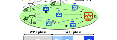
Figure 1: System model and frame structure.

The entire process is divided into two phases, i.e., a WPT phase and a WIT phase. During the WPT phase, instead of a single source, multiple WPT sources are utilized as energy suppliers in attempt to achieve a relatively higher energy efficiency. In particular, $M$ sources transmit mutually independent RF signals to $N$ sensors in a broadcasting manner, with possibly different transmit power which are denoted by $\{P_{j}\},\forall j=1,\cdots,M$. The blocklength (i.e., the amount of symbols) of the WPT phase is denoted by $m_{0}$, while the time duration of a single symbol is denoted by $T_{s}$. Consequently, the time length for WPT is $m_{0}T_{s}$. Since sufficient energy has been buffered from the surroundings by sources, a significant quantity of transmit power can be generated for WPT. This, coupled with the generally small packet size and correspondingly relatively little energy required for reliable WIT, results in a relatively short time length for performing WPT. Therefore, it is reasonable to consider the channel gains within WPT phase as constant. The channel gain between ${\rm{S}}_{j}$ and ${\rm{R}}_{i}$ is denoted by $z_{i,j}$. After receiving the independent RF signals from multiple WPT sources, the EH unit of each sensor converts them to DC signals and performs EH to supply sufficient energy for the forthcoming short packet transmission. We assume that the EH units’ EH capability is stable, i.e., the charged power at ${\rm{R}}_{i}$ is a constant and denoted by $Q_{\rm{ch},i},\forall i=1,\cdots,N$, such that the corresponding harvested energy during the whole WPT phase can be written as $Q_{\rm{ch},i}m_{0}T_{s}$.

During the WIT phase, $N$ short packets with sizes of $k_{i},\forall i=1,\cdots,N$ bits are transmitted to D from $N$ sensors by consuming the harvested energy. The WIT process is performed in a time-division duplex (TDD) manner, i.e., $N$ packets are sequentially transmitted to D, with which the co-channel interference introduced by multiple sensors can be avoided. To ensure timely and accurate transmission of the sensed data packets, low latency and high reliability WIT is required, which, coupled with the generally small data amount of the packets generated by IoT sensors, indicates that FBL codes have to be utilized for WIT. In the FBL regime, the decoding error probability cannot be ignored and the error probability of the transmission of each packet should be lower than 0.1 for guaranteeing ultra reliable communication, i.e., $\varepsilon_{i}\leq 0.1,\forall i=1,\cdots,N$ holds. Moreover, the entire duration of the WIT phase in symbol is restricted with $\sum_{i=1}^{N}m_{i}\leq m_{\rm{total}}$ , where $m_{i},\forall i=1,\cdots,N$ denotes the blocklength of the packet transmission from ${\rm{R}}_{i}$ to D and $m_{\rm{total}}$ specifies the maximum total amount of symbols permitted during the WIT phase. Note that each symbol has a fixed length of $T_{s}$. Hence, the blocklength restriction can be formulated as a time constraint that ensures the low-latency WIT, i.e., $\sum_{i=1}^{N}m_{i}T_{s}\leq m_{\rm{total}}T_{s}$. Since the channels are assumed to be independent and experience quasi-static fading and the blocklength of each packet transmission is relatively short, the channel gain is reasonably considered as a constant during one block and varies independently to the next, i.e., the channel gain between ${\rm{R}}_{i}$ to D can be denoted by $\bar{z}_{2,i},\forall i=1,\cdots,N$. The noise power level is given as $\sigma^{2}$.

In addition, note that each sensor will utilize all the harvested energy for short packet transmission (to maximize the utilization of the energy) and accordingly guarantee reliable transmission. In this regard, the transmit power of ${\rm{R}}_{i}$ is jointly restricted by the harvested energy during the WPT phase $Q_{\rm{ch},i}m_{0}T_{s}$ and the time length of its packet transmission $m_{i}T_{s}$, i.e., $\bar{P}_{i}=\frac{Q_{\rm{ch},i}m_{0}T_{s}}{m_{i}T_{s}}$, where $\bar{P}_{i}$ denotes the transmit power of ${\rm{R}}_{i}$ for the short packet transmission in the WIT phase.

As discussed above, multiple sources are responsible for providing power supplement to multiple sensors, hence ensuring reliable short packet transmissions. However, the practical energy conversion efficiency during the EH process is quite limited, necessitating characterization and optimal designs on the achievable reliability performance of the considered network.

II-B FBL Transmission Model

The data transmissions in the WIT phase are assumed to be carried via FBL codes. According to [39, 40], with error probability $\varepsilon$, signal-to-noise ratio (SNR) $\gamma$, and blocklength $m$, the coding rate is given by

$$\vspace{-.2cm}r\approx{\cal C}\left({\gamma}\right)-\sqrt{{\cal V}\left({\gamma}\right)/m}{Q^{-1}}\left(\varepsilon\right),$$ (1)

where ${\cal C}\left({\gamma}\right)\!=\!\log\left({1\!+\!{\gamma}}\right)$ and ${\cal V}\left({\gamma}\right)\!=\!\left(1\!-\!\frac{1}{{{\left({1\!+\!\gamma}\right)}^{2}}}\right){\log_{2}^{2}}e$ are the Shannon capacity and the channel dispersion, and $Q^{-1}(\cdot)$ is the reverse of $Q\left(x\right)\!=\!\int\nolimits_{x}^{\infty}{\frac{1}{{\sqrt{2\pi}}}}{e^{-{t^{2}}/2}}dt$, which represents the Gaussian $Q$-function. In the other way round, with the coding rate $r$, blocklength $m$ and SNR $\gamma$, the error probability can be expressed as

$$\vspace{-.2cm}\varepsilon={\cal P}\left(\gamma,r,m\right)\approx Q\left({\frac{{{\cal C}\left(\gamma\right)-r}}{{\sqrt{{\cal V}\left({\gamma}\right)/m}}}}\right).$$ (2)

II-C Nonlinear Energy Harvesting Model

During the EH process, the received RF signal can be converted to a DC signal for further EH. So far, several nonlinear EH models have been established to depict the EH process, such as piece-wise linear based nonlinear EH model [41] and curve fitting based nonlinear EH model [42]. Both of them are stochasticmodels, which are decided by the measurement data from practical EH circuits and require another experiment when changes take place in the circuit. In [43] an analytical EH model based on practical EH circuits components is investigated, in which the output DC of the EH unite is represented by a nonlinear implicit function with respect to the received RF power and the energy conversion efficiency is particularly poor with low or high input power due to the turn-on voltage and the reverse breakdown of the diode(s) used in the rectifier circuit. However, all the aforementioned nonlinear models only consider a single RF signal for EH. When it comes to multi-source WPT, multiple RF signals are transmitted simultaneously and the harvested energy is not the sum of harvested power over each single RF signal. Recently, an analytical EH model for a multi-source WPT system is investigated. According to [38], the harvested DC power of multi-source WPT with independent RF signals can be represented by

$$\vspace{-.1cm}P_{\rm{dc}}\triangleq F_{\rm{nl}}(\boldsymbol{Q})\approx\left(\frac{1}{a}W_{0}(ae^{aI_{\rm{s}}}\varphi(\mathbf{Q}))-I_{s}\right)^{2}\hat{R}_{\rm{L}},$$ (3)

where $\boldsymbol{Q}\triangleq\left({Q_{1},\cdots,Q_{M}}\right)$ represents the set of $M$ received RF signal powers. In addition, $W_{0}(\cdot)$ indicates the principle branch of Lambert $W$ function, which is the inverse relation of function $f(x)=xe^{x}$. Constant $a=\frac{\hat{R}_{\rm{L}}}{nv_{\rm{t}}}$, where $\hat{R}_{\rm{L}}$, $n$ and $v_{\rm{t}}$ represent the load resistance, the ideality factor and the thermal voltage respectively. $I_{s}$ is the reverse bias saturation current, which is ignored in linear EH model. Moreover, $\varphi(\mathbf{Q})$ is an explicit expression written as

$$\vspace{-.1cm}\varphi(\mathbf{Q})=I_{\rm{s}}+\sum_{i=1}^{n_{0}}\beta_{i}\sum_{\sum_{m\!=\!1}^{M}\!i_{\rm{m}}\!=i}\hat{\mathcal{C}}_{i,\{{i_{\rm{m}}}\}}~{}\prod_{m=1}^{M}Q_{m}^{i_{m}/2},$$ (4)

where $n_{0}$ denotes the truncation order, which affects the accuracy for modelling the nonlinearity. Constant $\beta_{i}=\bar{k_{i}}R_{\rm{ant}}^{\frac{i}{2}}$, where $\bar{k_{i}}=\frac{I_{s}}{i!(nv_{t})^{i}}$ and $R_{\rm{ant}}$ represents the matched antenna impedance. In constant $\hat{\mathcal{C}}_{i,\{{i_{\rm{m}}}\}}=\frac{M!}{\prod_{m=1}^{M}i_{m}!}\prod_{m=1}^{M}\lambda_{m,i_{m}}$, $\lambda_{m,i_{m}}$ denotes the constant waveform factor for unit power. Expression $\sum_{m=1}^{M}i_{m}=i$ represents that any non-negative sequence $\{i_{m}\}$ must have a sum of $i$. According to (3), we can learn that the harvested power and the EH efficiency are affected by the received RF power. More clearly, $\varphi(\mathbf{Q})$ in (3) depicts the multiple RF combining process and is directly influenced by the multiple RF signal powers $\boldsymbol{Q}\triangleq\left({Q_{1},\cdots,Q_{M}}\right)$ based on (4). Expression $\prod_{m=1}^{M}Q_{m}^{i_{m}/2}$ in (4) indicates that the interference between multiple received RF signals cannot be ignored and that such interference can make an either positive or negative effect on energy acquisition results, which makes multi-source WPT enabled communication considerably more challenging than that with a single WPT source. Therefore, a reasonable power allocation among multiple WPT sources is significantly essential for high energy conversion efficiency realization.

So far, we have stated the system model, the FBL transmission model and the nonlinear EH model. Following them, resource allocation designs will be proposed in the following sections.

III Power Allocation Among Multiple WPT Sources

In this section, we focus on the power allocation design under the fixed frame structure, i.e., the lengths of the WPT phase and WIT are given. We first characterize the relationship among the FBL reliability and the multiple source power. Based on the characterization, an efficient power allocation design is proposed to minimize the overall error probability under the total power constraint.

III-A FBL Reliability Characterization and Problem Formulation

During the WPT phase, $M$ sources transmit RF signals with power $\{P_{j}\},\forall j=1,\cdots,M$ to $N$ sensors simultaneously in a broadcasting manner. Accordingly, each sensor ${\rm{R}}_{i},\forall i=1,\cdots,N$ will receive a set of RF signals with power $\boldsymbol{Q_{i}}\triangleq(Q_{i,\text{1}},\cdots,Q_{i,j},\cdots,Q_{i,\text{M}})$, where $Q_{i,j}$ denotes the power exclusively obtained from ${\rm{S}}_{j}$ and is given as

$$\vspace{-.2cm}Q_{i,j}(P_{j})=P_{j}z_{i,j}.$$ (5)

However, the received RF power cannot be directly consumed, i.e., RF signals are required to be converted to DC signals via an EH process and the corresponding charged power is written as

$$\vspace{-.2cm}Q_{\rm{ch,}i}(\boldsymbol{P})=F_{\rm{nl}}\left(\boldsymbol{Q}_{i}(\boldsymbol{P})\right),$$ (6)

where $F_{\rm{nl}}(\cdot)$ characterizes the relationship between the harvested DC power and the received multiple RF power according to (3). With charged power $Q_{\rm{ch,}i}$, the corresponding harvested energy of ${\rm{R}}_{i}$ during WPT phase is given as $Q_{\rm{ch},i}m_{0}T_{s}$, which will be completely consumed in the following WIT phase. During the WIT phase, each sensor transfers short packet to D with transmit power $\bar{P}_{i},\forall i\in\{1,2,...,N\}$, which is limited by the harvested energy, i.e.,

$$\vspace{-.1cm}\bar{P}_{i}(Q_{\rm{ch,}i}(\boldsymbol{P}))=\frac{Q_{\rm{ch},i}(\boldsymbol{P})m_{0}T_{s}}{m_{i}T_{s}}=\frac{Q_{\rm{ch},i}(\boldsymbol{P})m_{0}}{m_{i}},\forall i\in\{1,2,...,N\},$$ (7)

where $m_{0}$ and $m_{i}$ are positive integers denoting the blocklengths respectively assigned for WPT and WIT (from ${\rm{R}}_{i}$ to D). Notation $T_{s}$ denotes the time length of a single symbol. As a result, the SNR of the transmission from ${\rm{R}}_{i}$ to D can be written as

$$\vspace{-.1cm}\gamma_{i}(\bar{P}_{i})=\frac{{\bar{P}_{i}}\bar{z}_{\rm 2,i}}{\sigma_{i}^{2}}.$$ (8)

Note that, with given channel gain $\bar{z}_{\rm 2,i}$, noise power $\sigma_{i}^{2}$, WPT blocklength $m_{0}$ and WIT blocklength $m_{i}$ (under fixed frame structure), the sensor transmit power ($\bar{P}_{i}$) as well as the SNR ($\gamma_{i}$) are directly and completely decided by the charged power ($Q_{\rm{ch},i}$) and both of which are complex nonlinear functions with respect to multiple source power $\{P_{j}\},\forall j=1,\cdots,M$ based on (6),  (7) and (8). In order to guarantee reliable transmission, we assume the network should guarantee $\gamma_{i}\geq 1$, which implies respectively direct and indirect limitations on $\bar{P}_{i}$ and $\{P_{j}\},\forall j=1,\cdots,M$.

According to (2), the FBL error probability of the transmission from ${\rm{R}}_{i}$ to D can be written as $\varepsilon_{i}={\cal P}\left(\gamma_{i},r_{i},m_{i}\right)$, where $r_{i}=\frac{k_{i}}{m_{i}}$. Clearly, with given packet size $k_{i}$ and WIT blocklength $m_{i}$, $\varepsilon_{i}$ is fully influenced by $\gamma_{i}$. Combined with (8), the transmission error probability from ${\rm{R}}_{i}$ to D can be written as

$$\vspace{-.1cm}\varepsilon_{i}(\bar{P}_{i})={\cal P}\left(\gamma_{i}(\bar{P}_{i}),r_{i},m_{i}\right).$$ (9)

Since all the packets are expected to be transferred with ultra reliability, the overall error probability is applied as the performance indicator for system investigation. $\varepsilon_{\text{O}}=1-\prod_{i=1}^{N}(1-\varepsilon_{i})$. As mentioned before, the error probability of transmission of each packet must be lower than 0.1 to guarantee reliable transmission, i.e., $\varepsilon_{i}\leq 0.1,\forall i\in\{1,2,...,N\}$. Hence, $\varepsilon_{i}+\varepsilon_{i^{\prime}}\gg\varepsilon_{i}\varepsilon_{i^{\prime}}$, $\forall i,{i^{\prime}}\in\{1,2,...,N\}$ holds, i.e., the high-order term $\varepsilon_{i}\varepsilon_{i^{\prime}}$ is negligible in comparison to $\varepsilon_{i}+\varepsilon_{i^{\prime}}$. As a result, the overall error probability can be tightly approximated to

$$\vspace{-.1cm}\varepsilon_{\text{O}}(\varepsilon_{i})=1-\prod_{i=1}^{N}(1-\varepsilon_{i})\approx\sum_{i=1}^{N}\varepsilon_{i}.$$ (10)

So far, the relationships among the overall error probability $\sum_{i=1}^{N}\varepsilon_{i}$, SNR $\boldsymbol{\gamma}$, sensor transmit power $\boldsymbol{\bar{P}}$ and source transmit power $\boldsymbol{P}$ have been characterized. Following the characterization, the power allocation problem minimizing the overall error probability is formulated as follow:

$$({\rm OP1}): \!\!{\min\limits_{\{\boldsymbol{P}\}}}\, \sum_{i=1}^{N}\varepsilon_{i}$$ (11a)

$$\rm{s.t.:} \frac{{\bar{P}_{i}}(Q_{\rm{ch,}i}(\boldsymbol{P}))\bar{z}_{\rm 2,i}}{\sigma_{i}^{2}}\geq\max\{1,2^{\frac{k_{i}}{m_{i}}}-1\},$$ (11d)

$$\sum_{j=1}^{M}P_{j}\leq P_{\rm{total}},$$

$$0\leq P_{j}\leq P_{\rm max},$$

where objective function (11a) presents the overall error probability, which has been tightly approximated as the sum of $N$ single link transmission error probabilities during the WIT phase accordingly to (10). In constraint (11d), term $\frac{{\bar{P}_{i}}(Q_{\rm{ch,}i}(\boldsymbol{P}))\bar{z}_{\rm 2,i}}{\sigma_{i}^{2}}$ represents the SNR of transmission from $\rm R_{i}$ to D. Constraint (11d) specifies that the coding rate should be smaller than the Shannon capacity, i.e., $\frac{k_{i}}{m_{i}}\leq\log_{2}(1+\bar{P}_{i}\frac{\bar{z}_{\rm 2,i}}{\sigma_{i}^{2}})$ and the SNR should be larger than 1 to guarantee reliable transmission. In (11d), total power consumption restriction is announced. Finally, (11d) announces the upper bound of the transmit power for each WPT source. By solving Problem (OP1), we can identify the optimal system reliability achievable under a given total power constraint and the corresponding optimal power allocation strategy.

However, Problem (OP1) is not convex. On the one hand, the objection function is not necessary convex, i.e., the convexity of error probability $\varepsilon_{i}$ to multiple source transmit power $\boldsymbol{P}$ is unpredictable since $\varepsilon_{i}$ is directly affected by the transmit power $\bar{P}_{i}$, which is a complex nonlinear function respect to $\boldsymbol{P}$. On the other hand, the convexity of constraint (11d) is also not guaranteed since term ${\bar{P}_{i}}(Q_{\rm{ch,}i}(\boldsymbol{P}))$ is not concave. As a result, Problem (OP1) is non-convex in its current form, which cannot be efficiently solved by standard convex programming methods..

III-B Problem Reformulation and SCA-based Solution

Based on prior analysis, original problem (OP1) is a complicated non-convex optimization problem due to the nonlinear EH process. To address this issue, we first introduce auxiliary variables and subsequently reformulate the original problem via the SCA algorithm.

Though $\varepsilon_{i}$ is not necessary convex to $\boldsymbol{P}$, the convex relationship between $\varepsilon_{i}$ and SNR $\gamma_{i}$ has been demonstrated in [44]. Moreover, recalling (7) and (8), $\gamma_{i}$ is clearly and fully determined by $\bar{P}_{i}$ in a linear form and $\bar{P}_{i}$ is fully affected by multiple source power, which motivates us to introduce $\boldsymbol{\bar{P}}$ as a new set of variables (to be optimized). In other words, as a set of intermediate variables, $\boldsymbol{\bar{P}}$ can decouple the complex nonlinear relationship between the error probability $\varepsilon_{i}$ and WPT source power $\boldsymbol{P}$ without modifying the original problem, which has the following two advantages: i. the equality function (6) is then converted to an inequality one, which enables the further application of SCA. ii. original nonlinear constraint (11d) (with respect to $\boldsymbol{P}$) becomes linear (wtih respect to $\bar{P}$). By this means, the reformulated problem is depicted as follows

$$({\rm P1}): \!\!{\min\limits_{\boldsymbol{P},\boldsymbol{\bar{P}}}}\, \sum_{i=1}^{N}\varepsilon_{i}$$ (12a)

$$\rm{s.t.} \bar{P}_{i}\leq F_{\rm{nl}}[\boldsymbol{Q}_{i}(\boldsymbol{P})]\frac{m_{0}}{m_{i}},$$

$$\frac{{\bar{P}_{i}}\bar{z}_{\rm 2,i}}{\sigma_{i}^{2}}\geq\max\{1,2^{\frac{k_{i}}{m_{i}}}-1\},$$

$$~{}\eqref{OP3.1con:sum P},\eqref{OP3.1con:upper P}.$$

First, we take a look at (12), which includes a sophisticated nonlinear EH process. According to [38], $Q_{\rm{ch,}i}$ is jointly convex in $\{\hat{Q}_{i,j}\}$ where $\hat{Q}_{i,j}=\frac{1}{Q_{i,j}},j=1,\cdots,M$. For ease of characterization, we define a set of new variables $\hat{\boldsymbol{P}}\triangleq\{\hat{P}_{\text{1}},\hat{P}_{\text{2}},\cdots,\hat{P}_{\text{M}}\}$, where $\hat{P_{j}}=\frac{1}{P_{j}},\forall{j}\in\{1,\cdots,M\}$. In particular, $\hat{Q}_{i,j}=\hat{P_{j}}\frac{1}{z_{i,j}}$, where $z_{i,j}$ is a positive constant. Note that $Q_{\rm{ch,}i}$ is jointly convex and apparently non-increasing in $\hat{Q}_{i,j}$, and $\hat{Q}_{i,j}$ is an affine function of $\hat{P_{j}}$. As a result, $Q_{\rm{ch,}i}=F_{\rm{nl}}[\boldsymbol{\hat{Q}}_{i}(\boldsymbol{\hat{P}})]$ is jointly convex in $\boldsymbol{\hat{P}}$ based on the convex property of the composite function. Therefore, constraint (12), (11d) and (11d) can be respectively reformed as,

$$\vspace{-.2cm}\bar{P}_{i}\leq F_{\rm{nl}}[\boldsymbol{Q}_{i}(\boldsymbol{\hat{P}})]\frac{m_{0}}{m_{i}},$$ (13)

$$\vspace{-.3cm}\sum_{j=1}^{M}\frac{1}{\hat{P_{j}}}\leq P_{\rm{total}},$$ (14)

$$\vspace{-.3cm}{\hat{P_{j}}}\geq\frac{1}{P_{\rm max}}.$$ (15)

However, constraint (13) is not convex due to the non-concave term $F_{\rm{nl}}[\boldsymbol{Q}_{i}(\boldsymbol{\hat{P}})]$. To address it, SCA is applied to convert the original non-convex constraint into a convex one. In particular, a concave function $\hat{P}_{\rm{ch},i}$ is required, which satisfies $F_{\rm{nl}}[\boldsymbol{Q}_{i}(\boldsymbol{\hat{P}})]\geq\hat{P}_{\rm{ch},i}$. Since $Q_{\rm{ch,}i}=F_{\rm{nl}}[\boldsymbol{Q}_{i}(\boldsymbol{\hat{P}})]$ has been proved being joint convex in $\boldsymbol{\hat{P}}$, an inequality can be obtained based on the property of convex function

$$\vspace{-.1cm}Q_{\rm{ch,}i}=F_{\rm{nl}}[\boldsymbol{Q}_{i}(\boldsymbol{\hat{P}})]\geq\sum_{j=1}^{M}-A^{(\tau)}_{i,j}\hat{P_{j}}+B^{(\tau)}_{i},\vspace{-.1cm}$$ (16)

where $A_{i,j}^{(\tau)}$ and $B_{i}^{(\tau)}$ are the positive constants defined as

$$\vspace{-.1cm}\begin{split}A_{i,j}^{(\tau)}&=\frac{\partial F_{\rm{nl}}[\boldsymbol{Q}_{i}(\boldsymbol{\hat{P}})]}{\partial\hat{P_{j}}}\mid_{\hat{P_{j}}=\hat{P_{j}}^{(\tau)}},\end{split}$$ (17)

$$\vspace{-.3cm}B_{j}^{(\tau)}=F_{\rm{nl}}[\boldsymbol{Q}_{i}(\boldsymbol{\hat{P}})]\mid_{\hat{P_{j}}=\hat{P_{j}}^{(\tau)}}+\sum_{j=1}^{M}A^{(\tau)}_{i,j}\hat{P_{j}},$$ (18)

and the equality in (16) holds at the local point $\boldsymbol{\hat{P}}^{(\tau)}$. Therefore, the non-concave term $F_{\rm{nl}}[\boldsymbol{Q}_{i}(\boldsymbol{P})]$ is approximated to a concave one $\sum_{j=1}^{M}-A^{(\tau)}_{i,j}\hat{P_{j}}+B^{(\tau)}_{i}$. Consequently, the original non-convex problem is approximated into a local subproblem, which can be solved iteratively until the stable point is achieved. In the $\tau$-th iteration, the corresponding subproblem can be written as

$$\!\!\!({\rm SP1}): \!\!\!\!\!\!{\min\limits_{\boldsymbol{\hat{P}},\boldsymbol{\bar{P}}}}\, \sum_{i=1}^{N}\varepsilon_{i}$$ (19a)

$$\rm{s.t.} \bar{P}_{i}\leq\frac{m_{0}}{m_{i}}\!\left(\sum_{j=1}^{M}-A^{(\tau)}_{i,j}\hat{P_{j}}+B^{(\tau)}_{i}\!\right)\!\!,$$

$$~{}\eqref{OP3.3P1con:SNR bound},\eqref{constraint hatP sum},\eqref{constraint hatP upper bound2}.$$

Afterwards, we propose the following lemma to prove the convexity of Subproblem (SP1).

Lemma 1.

Subproblem (SP1) is convex.

Proof.

We start the proof by verifying the convexity of all constraints. First, constraint (19) is conducted via the proposed convex approximation, which is convex. Second, (12) can be represented by two linear constraints, which are also convex. Third, for constraint (14) and  (15), clearly $\frac{1}{\hat{P_{j}}}$ is convex in $\hat{P_{j}}$. Noted that $\frac{1}{\hat{P_{j}}}$ is independent in $\hat{P_{j^{\prime}}},\forall{j^{\prime}}\neq j$ and $\boldsymbol{\bar{P}}$, thus $\frac{1}{\hat{P_{j}}}$ is joint convex in $(\boldsymbol{\hat{P}},\boldsymbol{\bar{P}})$. Therefore, $\sum_{j=1}^{M}\frac{1}{\hat{P_{j}}}$ is also convex.

Then, the major task to prove Lemma 1 becomes showing the convexity of the objective function. According to [44], while $\gamma\geq 1$, $\varepsilon_{i}$ is convex in $\gamma_{i}$, i.e., $\frac{\partial^{2}\varepsilon_{i}}{\partial\gamma_{i}^{2}}\geq 0$. Based on (8), both first and second derivatives of $\gamma_{i}$ are not negative, i.e., $\frac{\partial\gamma_{i}}{\partial\bar{P}_{i}}=\frac{\bar{z}_{\rm 2,i}}{\sigma_{i}^{2}}\geq 0,\frac{\partial^{2}\gamma_{i}}{\partial\bar{P}_{i}^{2}}=0.$ Therefore, the second derivative of $\varepsilon_{i}$ with respect to $\bar{P}_{i}$ is written as

$$\vspace{-.1cm}\begin{split}\frac{\partial^{2}\varepsilon_{i}}{\partial\bar{P}_{i}^{2}}&=\frac{\partial^{2}\varepsilon_{i}}{\partial\gamma_{i}^{2}}\left(\frac{\partial\gamma_{i}}{\partial\bar{P}_{i}}\right)^{2}\!+\frac{\partial\varepsilon_{i}}{\partial\gamma_{i}}\frac{\partial^{2}\gamma_{i}}{\partial\bar{P}_{i}^{2}}=\frac{\partial^{2}\varepsilon_{i}}{\partial\gamma_{i}^{2}}(\frac{\bar{z}_{\rm 2,i}}{\sigma_{i}^{2}})^{2}\,\geq\,0,\end{split}$$ (20)

which indicates that the error probability of single link transmission is convex in the transmit power of the corresponding sensor, i.e., $\varepsilon_{i}$ is convex in $\bar{P}_{i}$.

In addition, in the local subproblem, $\varepsilon_{i}={\cal P}\left(\gamma_{i}(\bar{P}_{i})\right)$, which is influenced by $\bar{P}_{i}$ but independent in $\bar{P}_{i^{\prime}},\forall i^{\prime}\neq i$, i.e., we have $\frac{\partial\varepsilon_{i}}{\partial\bar{P}_{i^{\prime}}}=0$, $\frac{\partial^{2}\varepsilon_{i}}{\partial\bar{P}_{i^{\prime}}^{2}}=0$, and $\frac{\partial^{2}\varepsilon_{i}}{\partial\bar{P}_{i}\partial\bar{P}_{i^{\prime}}}=0$, case $i^{\prime}\neq i$. Moreover, $\varepsilon_{i}$ is not affected by $\boldsymbol{\hat{P}}$ in the local subproblem. Hence, it can be shown that the Hessian matrix of $\varepsilon_{i}$ to $(\boldsymbol{\hat{P}},\boldsymbol{\bar{P}})$ has only one non-zero element $\frac{\partial^{2}\varepsilon_{i}}{\partial\bar{P}_{i}^{2}}\geq 0$, i.e., being semi-positive definite. In other words, $\varepsilon_{i}$ is jointly convex to $(\boldsymbol{\hat{P}},\boldsymbol{\bar{P}})$. As a sum of convex functions, the objective function of (SP1) is also jointly convex to $(\boldsymbol{\hat{P}},\boldsymbol{\bar{P}})$, and thus Subproblem (SP1) is convex. ∎

According to the lemma 1, Subproblem (SP1) can be efficiently solved and the flow of the proposed SCA-based solution is described in Algorithm 1. In Algorithm 1, we first initialize the values of transmit power $\boldsymbol{\hat{P}}^{(0)}$. In particular, we utilize an improved initial point (IIP) decision strategy to obtain the initial feasible solutions: 1) Based on the monotonic optimization programming tool, we obtained a set of minimum source power $\boldsymbol{P}_{\rm{min}}$ that satisfies the constraint (11b) in Original Problem (OP1), which is defined as basic initial point (BIP) decision strategy. 2) Calculate the remaining power that has not been allocated to sources (i.e., $P_{\rm{remaining}}=P_{\rm{total}}-\sum_{j=1}^{N}P_{\rm{min},j}$). 3) The remaining power is equally allocated to all WPT sources, i.e., the initialized transmit power of $\rm S_{j}$ is given as $P_{{\rm initial},j}=\min\{P_{\rm{min},j}+\frac{P_{\rm{remaining}}}{M},P_{\rm max}\}$. As a result, ${\hat{P}_{j}}^{(0)}=\frac{1}{P_{{\rm initial},j}}$. After initialization, the local problem (18) is addressed aiming at minimizing the overall error probability by optimizing $(\boldsymbol{\hat{P}},\boldsymbol{\bar{P}})$. In the $\tau$-th iteration, via solving the local problem, we determine the optimal solution $(\boldsymbol{\hat{P}}^{(\tau)},\boldsymbol{\bar{P}}^{(\tau)})$ of the problem. Subsequently, in the second step, a new local problem based on $(\boldsymbol{\hat{P}}^{(\tau)},\boldsymbol{\bar{P}}^{(\tau)})$ arises. Through the iteration repetition until convergence, an efficient sub-optimal solution to problem (P1) will be obtained.

Finally, we investigate the complexity of the proposed iteration algorithm based on the ellipsoid method. In problem (SP1), the number of optimization variables is $\left(M+N\right)$, resulting in $\mathcal{O}((M+N)^{2}\frac{1}{\epsilon})$ rounds of ellipsoid updates, where $\epsilon$ denotes the optimization threshold. During each round of ellipsoid update, the complexity cost for object function is $\mathcal{O}((M+N)^{2})$ and that for constraints is $\mathcal{O}((M+N)(N+N+M))$. Finally, with $\Phi$ rounds of iteration, the complexity of the proposed algorithm can be obtained as $\mathcal{O}\!\left(\!\Phi(M+N)^{2}\frac{1}{\epsilon}\!\right)\!\times\Big{(}\!\mathcal{O}(M+N)^{2}\!+\!\mathcal{O}\big{(}(M+N)(N+N+M)\big{)}\!\Big{)}=\mathcal{O}\left(\Phi(M+N)^{3}(M+2N)\frac{1}{\epsilon}\right)$.

Algorithm 1 Power Allocation Algorithm

  Initialization

  Initialize a feasible $(\boldsymbol{\hat{P}}^{(0)},\boldsymbol{\bar{P}}^{(0)})$.

  Initialize the overall error probability $\boldsymbol{\varepsilon_{\text{o}}}^{(0)}$ based on $(\boldsymbol{\hat{P}}^{(0)},\boldsymbol{\hat{P}}^{(0)})$.

   Iteration

  a)   $\varepsilon_{\text{o,min}}=\varepsilon_{\text{o}}^{(0)}$, $\boldsymbol{\hat{P}}_{\rm{opt}}=P^{(0)}$, $\boldsymbol{\bar{P}}_{\rm{opt}}=\bar{P}^{(0)}$, $\tau=0$

  b)   iteration number $\tau=\tau+1$

      for sensor $i=1:N$    for source $j=1:M$

  c)      Determine parameters $A_{ij}^{(\tau)}$ according to (17)

        endfor

  d)       Determine parameters $B_{i}^{(\tau)}$ according to (18)   endfor

  e)    Update $\boldsymbol{\hat{P_{j}}}^{(\tau+1)}$ and $\boldsymbol{\bar{P}_{i}}^{(\tau+1)}$ by solving (18)

  f)     if ${\left|\varepsilon_{\text{o}}^{{}_{({\rm\tau}+1)}}-\varepsilon_{\text{o,min}}\right|}\big{/}{\varepsilon_{\text{o,min}}}\leq\varepsilon_{\text{converge-threshold}}$

           break

       endif

  g)     if $\varepsilon_{\text{o}}^{({\rm\tau}+1)}<\varepsilon_{\text{o,min}}$

        $\varepsilon_{\text{o,min}}={\varepsilon_{\text{o}}^{({\rm\tau}+1)}}$, $\hat{P_{j}}={\hat{P_{j}}^{({\rm\tau}+1)}}$,

  h)    else jump to step b).

      endif

IV Joint Power and Blocklength Allocation

So far, a power allocation design with fixed frame structure has been completed in the previous section. In this section, our work is extended to the joint resource allocation design under scenarios with dynamic frame structure, namely the source power and blocklength allocated for WPT phase and short packets transmission phase are supposed to be jointly optimized for minimizing the overall error probability.

IV-A Problem Formulation

In contrast to fixed frame structure, dynamic frame structure permits flexible blocklength adjustment for better system performance achievement based on a variety of influencing factors, including channel states, packet size, transmit power, etc. Under such dynamic frame structure, we aim to minimize the overall error probability under both total power and total blocklength constraints. For this purpose, there exists a tradeoff with respect to the power and blocklength. Power allocation design has been discussed in section III, therefore we focus on the latter in this subsection. One the one hand, there exists a compromise between the blocklength allocated for WPT phase and WIT phase. Allocating more blocklength for WPT phase contributes to higher harvested energy, accordingly higher SNR based on (7) (8), which helps reduce the overall error probability according to (2), but the blocklength for WIT becomes shorter, which has negative impacts on the overall error probability. Allocating more blocklength for WIT phase can directly improve the FBL reliability according to (2), nevertheless, the harvested energy may become insufficient, i.e., the SNR becomes smaller, which makes negative impacts on system reliability. One the other hand, there also exists a tradeoff inside the WIT phase, involving the blocklength allocation among multiple sensors. For each sensor, a longer blocklength benefits its own short packet transmission, but the available blocklength for other sensors is reduced, which negatively affects other sensors’ reliable transmission. To guarantee the overall system reliability, each short packet must be transmitted reliably, since the overall error probability to some extent is likely to be determined by the worst transmission. In addition, although longer blocklength can directly reduce error probability based on (2), with given harvested energy, longer WIT blocklength results in lower sensor transmit power, namely lower SNR according to (7) (8), which again portrays the tradeoff regarding blocklength. Therefore, appropriate blocklength allocation design is of great importance to guarantee the system reliability in a multi-source WPT enabled multiple short packets transmission network. In order to minimize the overall error probability of the system, the joint power and blocklength optimization can be formulated as

$$({\rm OP2}): \!\!{\min\limits_{\{\boldsymbol{P}\},\{\boldsymbol{m}\},m_{0}}}\, \sum_{i=1}^{N}\varepsilon_{i}$$ (21a)

$$\rm{s.t.:} m_{0}+\sum_{i=1}^{N}m_{i}\leq m_{\rm{total}},$$

$$\frac{{\bar{P}_{i}}(Q_{\rm{ch,}i}(\boldsymbol{P}),m_{i},m_{0})\bar{z}_{\rm 2,i}}{\sigma_{i}^{2}}\geq\max\{1,2^{\frac{k_{i}}{m_{i}}}-1\},$$

$$\eqref{3.1 barP},\eqref{OP3.1con:sum P},{\eqref{OP3.1con:upper P}},$$

where constraint (21) announces the upper bound of total blocklength (latency) of the whole network. To facilitate the problem settlement, we utilize the integer relaxation strategy to treat variables $m_{0}$ and $\boldsymbol{m}$ as continuous variables, i.e., $m_{0},\boldsymbol{m}\in\mathbb{R}$. In (21), term ${\bar{P}_{i}}(Q_{\rm{ch,}i}(\boldsymbol{P}),m_{i},m_{0})$ indicates the transmit power of $R_{i}$, which is jointly affected by $\boldsymbol{P}$, $m_{i}$ and $m_{0}$. In (7), relationship between $\boldsymbol{P}$ and $\bar{P}_{i},\forall i=1,\cdots,N$ is depicted. Constraints (11d) and (11d) respectively announce the total power consumption restriction and the upper bound of transmit power for each WPT source. Recalling (2), i.e., $\varepsilon_{i}={\cal P}\left(\gamma_{i},r_{i},m_{i}\right)$, with given packet size $k_{i}$, the single link transmission error probability $\varepsilon_{i}$ in (21a) is jointly influenced by $\left(\gamma_{i},m_{i}\right)$. Combining (6), (8), the error probability of the transmission from $\rm{R}_{j}$ to D can be written as

$$\varepsilon_{i}(\boldsymbol{P},m_{i},m_{0})={\cal P}\left(\gamma_{i}\left(\bar{P}_{i}\left(\boldsymbol{P},m_{i},m_{0}\right)\right),r_{i},m_{i}\right).$$ (22)

Clearly, the nonlinearity in EH process, as well as the complicated Q-function in FBL model, have made Problem (OP2) nonconvex and intractable. In particular, when the WPT source power levels are supposed to be jointly optimized with the blocklength, the joint convexity of $\varepsilon_{i}$ can hardly be expected with respect to $(\boldsymbol{P},\boldsymbol{m})$. Furthermore, the adjustable blocklengths for both WPT and WIT phases are coupled, i.e., having particularly resulted in significant joint impacts on the transmit power $\bar{P}_{i}(\boldsymbol{P},m_{i},m_{0})$ and subsequently on the error probability $\varepsilon_{i}$, which has introduced extreme analysis difficulty in addressing Problem (OP2).

IV-B Efficient Solution to Problem (OP2)

In this subsection, we provide a SCA-based approach efficiently addressing Problem (OP2) via two steps: First, we decouple the complex relations between the WPT and WIT phases by introducing auxiliary variables, which results in a reformulation to Problem (OP2) ; Subsequently, we characterize the reformulated problem, especially the reformulated constraints, and conducting corresponding convex approximations.

On the first step, we decouple the complicated relationship between the error probability $\varepsilon_{i}$ in the WIT phase and the resource allocation decision in the WPT phase $\{\boldsymbol{P},m_{0}\}$, while maintaining such coupled relationship in constraints. In particular, we introduce auxiliary power variables $\boldsymbol{\bar{P}}$ to be optimized and establish a new coupling relation between $\varepsilon_{i}$ and ${\bar{P}_{i}}$, where ${\bar{P}_{i}}$ is the transmit power of $\rm R_{i}$ for short packet transmission. Therefore, (22) is rewritten as

$$\varepsilon_{i}(\bar{P}_{i},m_{i})={\cal P}\left(\gamma_{i}\left(\bar{P}_{i}\right),r_{i},m_{i}\right),$$ (23)

where error probability $\varepsilon_{i}$ is completely influenced by $(\bar{P}_{i},m_{i})$ and is independent from $P_{j},\forall j=1,\cdots,M$. This step reduces the number of variables that have a direct affection on $\varepsilon_{i}$ (from $M+2$ to $2$), thus simplifies the original complex relationship.

To guarantee the consistency of the upcoming reformulated problem and the original problem, the following inequality limitation between new optimization variables $\boldsymbol{\bar{P}}$ and original optimization variables $\boldsymbol{P},\boldsymbol{m},m_{0}$ must be satisfied,

$$\bar{P}_{i}m_{i}\leq F_{\rm{nl}}[\boldsymbol{Q}_{i}(\boldsymbol{P})]m_{0},\forall{i=1,\cdots,N},$$ (24)

which represents that the total consumed energy for short packet transmission during WIT phase should be no larger than the total harvested energy during WPT phase. Considering the monotonic increment property of FBL reliability with respect to sensor transmit power $\bar{P}$ and WIT blocklength $m$, the optimal reliability can be achieved only when all the resources (including power and blocklength) have been fully utilized and no remaining resource exists, i.e., the equality in (24) holds, which indicates the equivalence of inequality constraint (24) and the original equation constraint on the optimal solution to the problem.

To facilitate the problem solving, we utilize the same variable substitution in Subproblem (SP1), i.e., $\hat{P}_{i}=\frac{1}{P_{i}},i\in\{1,\cdots,N\}$, which is conducive to the further utilization of SCA. As a result, we obtained the reformulated problem (P3) after performing the decoupling step.

$$\!\!\!({\rm P3}): \!\!\!\!\!\!{\min\limits_{\boldsymbol{\hat{P}},\boldsymbol{\bar{P}},\boldsymbol{m},m_{0}}}\, \sum_{i=1}^{N}\varepsilon_{i}$$ (25a)

$$\rm{s.t.} \bar{P}_{i}m_{i}-m_{0}F_{\rm{nl}}[\boldsymbol{Q}_{i}(\boldsymbol{\hat{P}})]\leq 0,\forall{i,\cdots,N},$$

$$~{}\eqref{OP3.3P1con:SNR bound},\eqref{constraint hatP sum},\eqref{constraint hatP upper bound2},\eqref{4.1OPcon:sum m},$$

Clearly, problem (P3) is not convex as constraint (25) is non-convex to variables $\boldsymbol{\bar{P}},\boldsymbol{P},\boldsymbol{m},m_{0}$.

On the second step, we efficiently solve Problem (P3) via applying the SCA technique. In particular, we provide convex approximations to the problem by specifically addressing the nonlinear EH impact as well as the nonconvex term of products over variables in constraint (25), respectively.

On the one hand, we focus on the aforementioned difficulty introduced by nonlinear EH process, we utilize the similar method in Section III-B to convert $F_{\rm{nl}}[\boldsymbol{Q}_{i}(\boldsymbol{P})]$ into a simple linear form. Namely, we first perform variable substitution $\hat{P}_{j}=\frac{1}{P_{j}},\forall{j=1,\cdots,M}$. Then, based on the joint convexity relationship between $F_{\rm{nl}}[\boldsymbol{Q}_{i}(\boldsymbol{\hat{P}})]$ and $\boldsymbol{\hat{P}}$ (discussed in Section III-B), the term $F_{\rm{nl}}[\boldsymbol{Q}_{i}(\boldsymbol{\hat{P}})]$ is reformulated into a linear one, i.e., $\left(\sum_{j=1}^{M}-A^{(\tau)}_{i,j}\hat{P_{j}}+B^{(\tau)}_{i}\!\right)$, where $A^{(\tau)}_{i,j}$ and $B^{(\tau)}_{i}$ can respectively obtained by (17) (18), based on which constraint (25) is reformulated as

$$\bar{P}_{i}m_{i}-m_{0}\left(\sum_{j=1}^{M}-A^{(\tau)}_{i,j}\hat{P_{j}}+B^{(\tau)}_{i}\!\right)\leq 0,\forall{i,\cdots,N}.$$ (26)

On the other hand, constraint (26) is still nonconvex. Then, the remaining task is to further conduct convex approximation to constraint (26), while guaranteeing the convexity of other constraints in Problem (P3). To this end, we introduce the following variable substitution, i.e., set $\tilde{P}_{i}=\sqrt{\bar{P}_{i}},\tilde{m}_{i}=\frac{1}{m_{i}},\forall{i=1,\cdots,N}$. Thus, non-convex term $\bar{P}_{i}m_{i}$ in constraint (26) is converted into a convex form, i.e., $\frac{\tilde{P}^{2}_{i}}{\tilde{m}_{i}}$. For $-m_{0}\!\left(\sum_{j=1}^{M}-A^{(\tau)}_{i,j}\hat{P_{j}}+B^{(\tau)}_{i}\!\right)$, since $m_{0}$ is guaranteed to be positive and $\left(\sum_{j=1}^{M}-A^{(\tau)}_{i,j}\hat{P_{j}}+B^{(\tau)}_{i}\!\right)$ represents the charged power, which is also positive. Thus, based on the inequality of arithmetic and geometric means, i.e., $ab\leq\frac{1}{2}a^{2}+\frac{1}{2}b^{2}$ holds $\forall a,b\in\mathcal{R}^{+}$ and the equality holds when $a=b$, we can obtain that

$$-m_{0}\left(\sum_{j=1}^{M}-A^{(\tau)}_{i,j}\hat{P_{j}}+B^{(\tau)}_{i}\right) =\frac{m_{0}}{C_{i}^{(\tau)}}C_{i}^{(\tau)}\sum_{j=1}^{M}A^{(\tau)}_{i,j}\hat{P_{j}}-B^{(\tau)}_{i}m_{0}$$ (27)

$$\leq\frac{1}{2C_{i}^{(\tau)}}m_{0}^{2}+\frac{1}{2}C_{i}^{(\tau)}\left(\sum_{j=1}^{M}A^{(\tau)}_{i,j}\hat{P_{j}}\right)^{2}-B^{(\tau)}_{i}m_{0},$$

where the positive constant $C_{i}^{(\tau)}$ is given by

$$C_{i}^{(\tau)}=\frac{m_{0}^{(\tau)}}{\sum_{j=1}^{M}A^{(\tau)}_{i,j}\hat{P}_{j}^{(\tau)}},$$ (28)

which guarantees the equality in (27) holds at the local point $(\hat{P}_{j}^{(\tau)},m_{0}^{(\tau)})$. Obviously, both expression $\frac{1}{2C_{i}^{(\tau)}}m_{0}^{2}$ and $-B^{(\tau)}_{i}m_{0}$ are convex. Then, we investigate the convexity of $\frac{1}{2}C_{i}^{(\tau)}\left(\sum_{j=1}^{M}A^{(\tau)}_{i,j}\hat{P_{j}}\right)^{2}.$ Expression $\frac{1}{2}C_{i}^{(\tau)}\left(\sum_{j=1}^{M}A^{(\tau)}_{i,j}\hat{P_{j}}\right)^{2}$ is convex and monotonically increasing in $\Theta_{i}$, where $\Theta_{i}=\sum_{j=1}^{M}A^{(\tau)}_{i,j}\hat{P_{j}}$ and $A^{(\tau)}_{i,j}\geq 0$ , $\hat{P_{j}}\geq 0$. Moreover, expression $\Theta_{i}=\sum_{j=1}^{M}A^{(\tau)}_{i,j}\hat{P_{j}}$ is linear, which is jointly convex in $\hat{\boldsymbol{P}}$. According to the convexity preserving property of composite functions, expression $\frac{1}{2}C_{i}^{(\tau)}\left(\sum_{j=1}^{M}A^{(\tau)}_{i,j}\hat{P_{j}}\right)^{2}$ is jointly convex in $\hat{\boldsymbol{P}}$. As a result, non-convex constraint (26) can be reformulated into a convex one.

However, as a consequence of applying the above variable substitution, original convex constraint (12) becomes a non-convex one

$$\frac{\bar{z}_{2,i}}{\sigma_{i}^{2}}\tilde{P}^{2}_{i}\geq\max\{1,2^{k_{i}\hat{m_{i}}}-1\},$$ (29)

which further needs to be reformulated to a convex form. We achieve this by dividing constraint (29) into two constraints

$$\tilde{P}_{i}\geq\sqrt{\frac{\sigma_{i}^{2}}{\bar{z}_{2,i}}},$$ (30)

$$k_{i}\tilde{m_{i}}-\log_{2}(1+\tilde{P_{i}}^{2}\frac{\bar{z}_{2,i}}{\sigma_{i}^{2}})\leq 0,$$ (31)

where (30) is linear and convex with given $\sigma_{i}^{2},\bar{z}_{2,i}$. Obviously, $k_{i}\tilde{m_{i}}$ is linear and convex. Thus, the follwing task is to prove the convexity of $-\log_{2}(1+\tilde{P_{i}}^{2}\frac{\bar{z}_{2,i}}{\sigma_{i}^{2}})$. The second-order derivative of $-\log_{2}(1+\tilde{P_{i}}^{2}\frac{\bar{z}_{2,i}}{\sigma_{i}^{2}})$ can be given as

$$\begin{split}\frac{\partial^{2}[-\log_{2}(1+\tilde{P_{i}}^{2}\frac{\bar{z}_{2,i}}{\sigma_{i}^{2}})]}{\partial\tilde{P_{i}}^{2}}&=\frac{-2\ln 2\frac{\bar{z}_{2,i}}{\sigma_{i}^{2}}(1-\tilde{P_{i}}^{2}\frac{\bar{z}_{2,i}}{\sigma_{i}^{2}})}{[(1+\tilde{P_{i}}^{2}\frac{\bar{z}_{2,i}}{\sigma_{i}^{2}})\ln 2]^{2}},\end{split}$$ (32)

where term $(1-\tilde{P_{i}}^{2}\frac{\bar{z}_{2,i}}{\sigma_{i}^{2}})$ is non-positive when $\gamma_{i}\geq 1$, i.e., $\tilde{P_{i}}^{2}\frac{\bar{z}_{2,i}}{\sigma_{i}^{2}}\geq 1$ holds, which has been guaranteed in (30). Therefore, the second-order derivative of $-\log_{2}(1+\tilde{P_{i}}^{2}\frac{\bar{z}_{2,i}}{\sigma_{i}^{2}})$ is nonnegative and thus constraint (31) is convex.

Based on the above designed convex approximations and analysis, i.e., from (26) to (32), Problem (P3) can be solved via a SCA-based approach. In particular, in the $\tau$-th iteration of the approach, the local subproblem can formulated as

$$({\rm SP3}): \!\!{\min\limits_{\{\hat{P}_{j}\},\{\tilde{P}_{i}\},\{\tilde{m}_{i}\},{m_{0}}}}\, \sum_{i=1}^{N}\varepsilon_{i}(\tilde{P}_{i},\tilde{m}_{i})$$ (33a)

$$\rm{s.t.:} \frac{\tilde{P}^{2}_{i}}{\tilde{m}_{i}}+{\frac{1}{2C_{i}^{(\tau)}}m_{0}^{2}+\frac{1}{2}C_{i}^{(\tau)}\left(\sum_{j=1}^{M}A^{(\tau)}_{i,j}\hat{P_{j}}\right)^{2}-B^{(\tau)}_{i}m_{0}}\leq 0,$$ (33g)

$$\tilde{P}_{i}\geq\sqrt{\frac{\sigma_{i}^{2}}{\bar{z}_{2,i}}},$$

$$k_{i}\tilde{m_{i}}\leq\log_{2}(1+\tilde{P_{i}}^{2}\frac{\bar{z}_{2,i}}{\sigma_{i}^{2}}),$$

$$\sum_{j=1}^{M}\frac{1}{\hat{P_{j}}}\leq P_{\rm{total}},$$

$${\hat{P_{j}}}\geq\frac{1}{P_{\rm max}},$$

$$m_{0}+\sum_{i=1}^{N}\frac{1}{\tilde{m_{i}}}\leq m_{\rm{total}}.$$

Then, we provide the following key lemma for addressing Problem (SP3).

Lemma 2.

Problem (SP3) is convex.

Proof.

First, we prove the convexity of the object function. According to [45], the FBL reliability is joint convex in the root of transmit power and the reciprocal of blocklength, i.e., $\varepsilon_{i}$ is joint convex in $(\tilde{P}_{i},\tilde{m}_{i})$, where $\tilde{P}_{i}=\sqrt{\bar{P}_{i}}$ and $\tilde{m}_{i}=\frac{1}{m_{i}}$. Moreover, $\varepsilon_{i}$ is affected by $(\tilde{P}_{i},\tilde{m}_{i})$ but independent in $\tilde{P}_{i^{\prime}},\tilde{m}_{i^{\prime}},\forall{i^{\prime}\neq i}$, i.e., we have $\frac{\partial^{2}\varepsilon_{i}}{\partial\tilde{P}_{i^{\prime}}^{2}}=0$, $\frac{\partial^{2}\varepsilon_{i}}{\partial\tilde{m}_{i^{\prime}}^{2}}=0$, $\frac{\partial^{2}\varepsilon_{i}}{\partial\tilde{P}_{i}\tilde{P}_{i^{\prime}}}=0$, $\frac{\partial^{2}\varepsilon_{i}}{\partial\tilde{P}_{i}\tilde{m}_{i^{\prime}}}=0$, $\frac{\partial^{2}\varepsilon_{i}}{\partial\tilde{m}_{i}\tilde{P}_{i^{\prime}}}=0$, $\frac{\partial^{2}\varepsilon_{i}}{\partial\tilde{m}_{i}\tilde{m}_{i^{\prime}}}=0$. In addition, $\varepsilon_{i}$ is not affected by $\boldsymbol{\hat{P}}$ in the local sub-prblem. Therefore, in the Hessian matrix of $\varepsilon_{i}$ to $(\boldsymbol{\hat{P},\boldsymbol{\tilde{P}},\boldsymbol{m}},m_{0})$, only elements $\frac{\partial^{2}\varepsilon_{i}}{\partial\tilde{P}_{i}^{2}}$, $\frac{\partial^{2}\varepsilon_{i}}{\partial\tilde{m}_{i}^{2}}$,$\frac{\partial^{2}\varepsilon_{i}}{\partial\tilde{P}_{i}\partial\tilde{m}_{i}}$ are non-zero elements and $\frac{\partial^{2}\varepsilon_{i}}{\partial\tilde{m}_{i}^{2}}\frac{\partial^{2}\varepsilon_{i}}{\partial\tilde{m}_{i}^{2}}-(\frac{\partial^{2}\varepsilon_{i}}{\partial\tilde{P}_{i}\partial\tilde{m}_{i}})^{2}\geq 0$ is satisfied according to [45], i.e., the Hessian matrix is semi-positive definite. It indicates that $\varepsilon_{i}$ is joint convex in $(\boldsymbol{\hat{P},\boldsymbol{\tilde{P}},\boldsymbol{m}},m_{0})$. As a sum of convex functions, the object function $\sum_{i=1}^{N}\varepsilon_{i}$ is also joint convex in $(\boldsymbol{\hat{P},\boldsymbol{\tilde{P}},\boldsymbol{m}},m_{0})$.

Subsequently, we move on to prove the convexity of all constraints. Since term $\frac{\tilde{P}^{2}_{i}}{\tilde{m}_{i}}$ is jointly convex in $(\tilde{P}_{i},\tilde{m}_{i})$ and independent in $(\boldsymbol{\hat{P}},\tilde{P}_{i^{\prime}},\tilde{m}_{i^{\prime}},m_{0}),\forall{i^{\prime}\neq{i}}$, term $\frac{\tilde{P}^{2}_{i}}{\tilde{m}_{i}}$ is jointly convex in $(\boldsymbol{\hat{P}},\boldsymbol{\tilde{P}},\boldsymbol{\tilde{m}},m_{0})$. Moreover, constraint (33g) is obtained from convex approximation, which is also convex. Constraint (33g) and (33g) are the reformulated convex constraints, whose convexity have been proved in the previous discussion. Constraint (33g) and (33g) are the sum of convex functions, which are also convex. As the result, the object function and all constraints are all convex, thus the convexity of (SP3) is proved. ∎

Finally, a joint transmit power and blocklength design is depicted in Algorithm 2. In particular, we first initialize the value of $(\boldsymbol{\hat{P}^{(0)}},\boldsymbol{\tilde{P}^{(0)}},\boldsymbol{\tilde{m}^{(0)}},m_{0}^{(0)})$, utilizing the similar strategy for Algorithm 1, i.e., first finding the minimum $\boldsymbol{P}_{\rm{min}},\boldsymbol{m}_{\rm{min}},m_{0,\rm{min}}$ satisfying constraint (21C) in Original Problem (OP2) and subsequently equally allocating the remaining power and blocklength resources respectively among sources and among WPT and multi-packet transmissions during WIT. Subsequently, in the $\tau$-th iteration, we make out the constant parameters $A_{ij}^{(\tau)},B_{i}^{(\tau)},C_{i}^{(\tau)}$, solve Subproblem (SP3) and obtain the optimal solution $\hat{P}_{j}^{(\tau)}$, $\tilde{P}_{i}^{(\tau)}$, $\tilde{m}_{i}^{(\tau)}$, $m_{0}^{(\tau)}$. Then, in the second iteration, a new local problem based on $\hat{P}_{j}^{(\tau)}$, $\tilde{P}_{i}^{(\tau)}$, $\tilde{m}_{i}^{(\tau)}$, $m_{0}^{(\tau)}$ arises. Through repetition, an efficient sub-optimal solution to Problem (OP2) is converged. Based on the ellipsoid method, the computational complexity of Algorithm 2 is given as $\mathcal{O}\!\left(\!\Phi(M+2N+1)^{2}\frac{1}{\epsilon}\!\right)\!\times\Big{(}\!\mathcal{O}(M+2N+1)^{2}\!+\!\mathcal{O}\big{(}(M+2N+1)(M+3N+2)\big{)}\!\Big{)}=\mathcal{O}\left(\Phi(M+2N+1)^{4}\frac{1}{\epsilon}\right)$.

Algorithm 2 Joint Power and Blocklength Allocation Algorithm

  Initialization

  Initialize a feasible $(\boldsymbol{\hat{P}}^{(0)},\boldsymbol{\tilde{P}}^{(0)},\boldsymbol{\tilde{m}}^{(0)},m_{0}^{(0)})$.

  Initialize the overall error probability $\boldsymbol{\varepsilon_{\rm{o}}}^{(0)}$ based on $(\boldsymbol{\hat{P}}^{(0)},\boldsymbol{\tilde{P}}^{(0)},\boldsymbol{\tilde{m}}^{(0)},m_{0}^{(0)})$.

   Iteration

  a)   $\varepsilon_{\rm{o,min}}=\varepsilon_{\rm{o}}^{(0)}$, $\boldsymbol{\hat{P}_{\rm{opt}}}=\boldsymbol{\hat{P}^{(0)}}$, $\boldsymbol{\tilde{P}_{opt}}=\boldsymbol{\tilde{P}^{(0)}},\boldsymbol{\tilde{m}_{opt}}=\boldsymbol{\tilde{m}}^{(0)},m_{0,opt}=m_{0}^{(0)}$

  b)   for iteration number $\tau=$1:itern

       for sensor $i$=1:N    for source $j$=1:M

  c)      Determine parameters $A_{ij}^{(\tau)}$ according to (17)

        endfor

  d)    Determine parameters $B_{i}^{(\tau)}$ according to (18)

  e)    Determine parameters $C_{i}^{(\tau)}$ according to (28)    endfor

  f)    Update $\boldsymbol{\hat{P}}^{(\tau+1)}$, $\boldsymbol{\tilde{P}}^{(\tau+1)}$, $\boldsymbol{\tilde{m}}^{(\tau+1)}$, $m_{0}^{(\tau+1)}$ by solving (SP3)

  g)    if ${\left|\varepsilon_{\text{o}}^{{}_{({\rm\tau}+1)}}-\varepsilon_{\text{o,min}}\right|}\big{/}{\varepsilon_{\text{o,min}}}\leq\varepsilon_{\text{converge-threshold}}$

           break

        endif

  h)      if $\varepsilon_{o}^{({\rm itern}+1)}<\varepsilon_{o,min}$

  i)      then $\varepsilon_{o,min}={\varepsilon_{o}^{({\rm itern}+1)}}$, $\boldsymbol{\hat{P}_{opt}}=\boldsymbol{\hat{P}}^{({\rm itern}+1)}$,        $\boldsymbol{\tilde{P}_{opt}}=\boldsymbol{\tilde{P}}^{({\rm itern}+1)},\boldsymbol{\tilde{m}_{opt}}=\boldsymbol{\tilde{m}}^{({\rm itern}+1)}$, $m_{0,opt}=m_{0}^{({\rm itern}+1)}$

       endif

      endfor

V Numerical Results

In this section, we validate our proposed resource allocation designs and evaluate the system reliability via simulations. Unless specifically mentioned otherwise, the parameter setups of all the simulations are given as follows: D is located at (0,0) in the Cartesian coordinate. Three WPT sources are deployed on an arc $20$ meters from the D. Five sensors are evenly distributed on a circle with radius $2$ meters and the center at $(-15,-15)$. Blocklength of WPT phase and WIT phase are respectively set to $m_{0}=500$ and $m_{\rm{total}}=2000$. The duration of a single symbol is set to $T_{s}=66.7\mu s$. The upper bound of the transmit power for each WPT source is set to $30dBm$. The sizes of short packets are set to $90$ bits and the noise power is set to $-100\rm dBm$. About channel gains, we consider the Rayleigh distribution with the scale factor $\sigma=1$. With respect to the EH process, the parameter setups are adopted based on the circuit components from [46]: the reverse bias saturation current at diode is set to $I_{\rm s}=5\mu A$, the load resistance is set to $\hat{R_{\rm L}}=200\Omega$, and the truncation order is set to $n_{0}=4$. The diode ideality factor $n=1.05$ and thermal voltage $v_{t}=25.86mV$. Constants $a=7.37\times 10^{-3}\rm A^{-1}$, $\beta_{2}=0.6782,\beta_{4}=1.53\times 10^{4}$. Waveform factors are set as $\lambda_{j,2}=1,\lambda_{j,4}=1.5,\forall j\in\{1,\cdots,M\}$. In addition, it is worth mentioning that the blocklength optimization results (fractional solutions) have been converted to the integers (closest to the fractional solutions). Considering that the practical short blocklength for short packet communication is usually larger than 100 and even much larger, converting our results to integers will only have very minor effects on system reliability performance.

V-A Validation

We start with Fig. 2 to validate the optimality and the convergence performance of our proposed power allocation (IP) and joint resource allocation algorithm (PD). The impact of initial feasible points on optimality is also investigated. Optimal results obtained from exhaustive search (ES) are provided for comparison. Considering the high complexity of the exhaustive search algorithm, only 3 sensors are set for short packet transmission. In Fig. 2, ‘BIP’ and ‘IIP’ respectively represent the basic initial point decision regime and the improved initial points decision regime (introduced in Section III and Section IV). Obviously, the overall error probability of iterative algorithms gradually declines as the iteration progresses and the result converges after around 10 rounds of iteration, which indicates the high efficiency of our algorithms. Moreover, the results of our proposed iterative algorithm converge to a point, which is very close to the global optimal solution obtained by ES algorithm. In particular, the overall error probability gap between ‘IIP’ and ‘ES’ are 4.2710e-07 and 6.9300e-09 respectively for power allocation design (IP) and joint power and blocklength allocation (PD), which indicates the optimality of our design. The results also verify the equivalence of the optimal solutions to the original problem and the slacked one. Moreover, by comparing ‘BIP’ and ‘IIP’, we can learn that the suboptimal solutions obtained by the two regimes (with different initial feasible points) are very close, but ‘IIP’ converges with relatively fewer iteration number. This result indicates that different initial points will lead to different converge speed but only slight differences in the corresponding suboptimal solutions, which implies a high adaptability of our proposed algorithm with respect to initializations.

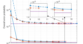
Figure 2: Optimality and convergence performance validation.

Subsequently, we intend to validate the necessity of utilizing the nonlinear EH model to portray the EH process. Fig. 3 depicts the power allocation results based on both linear and nonlinear EH model with given WPT blocklength and WIT blocklength, thus the impact of blocklength on system performance can be circumvented. In Fig. 3, ‘LPA’ and ‘NPA’ respectively indicate the linear EH model based power allocation and the nonlinear EH model based power allocation. ‘Actual Error’ refers to the practical overall error probability of LPA, i,e., the specific values of multi-source power (obtained from LPA) are brought into the nonlinear EH model to calculate the corresponding practical error probabilities based on (2). As shown in the figure, the reliability gap between ‘LPA’ and ‘NPA’ is less than half order of magnitude. However, ‘LPA’ is too idealistic, whose overall error probability is over two orders of magnitude lower than the actual result. This can be explained by the fact that the energy conversion efficiency in the actual EH model initially increases and subsequently declines as the received power increases due to the turn-on voltage and the reverse breakdown of the diode(s) utilized in the rectifier circuit. Nevertheless, linear model fails to accurately model the above nonlinear behavior due to the ideal and simplistic assumption of the constant conversion efficiency. Therefore, the resource allocation solutions based on the linear EH model have a significant likelihood of not being practically optimal, especially in multi-source wireless powered communication networks, where the received RF signals at each sensor may fluctuate significantly to each other due to diverse channel gains. More interestingly, when WIT blocklength increases from 1000 bits to 1800 bits, curve LPA first decreases slowly then the rate of decline fastens.

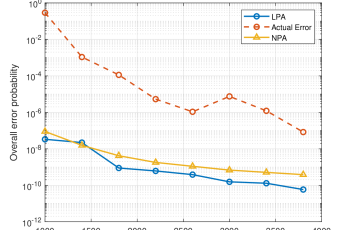
Figure 3: Comparison of system performance based on the linear and nonlinear EH models.

However, the situation is reversed for the ‘actual error’. The reason could be that under the linear EH model, more power is allocated to the ‘most suitable sources’ compared with the nonlinear one. Nevertheless, while incorporating the above resource allocation solutions into the nonlinear EH model, practical reliability enhancement might be much lower compared with the ideal linear one and even a negative influence may be brought to system performance (inverse increase of error at 3000 blocklength in ‘Actual Error’) since energy efficiency is rather lower with relatively higher received power. As a result, with same resource allocation setups, linear and nonlinear models may lead to rather different or even opposite performance trends. Beyond that, it can also be observed that the ‘NPA’ curve first decreases then flattens as the WIT blocklength increases. On the one hand, larger WIT blocklength directly contributes to lower the error probability. On the other hand, with certain energy harvested in the WPT phase, a longer WIT blocklength actually leads to a lower WIT transmit power and accordingly results in a lower SNR, which further negatively contributes to the reliability. In other words, the results also provide an insight into the tradeoff introduced by WIT blocklength, which indicates that increasing the WIT blocklength is not always an efficient way to improve the reliability.

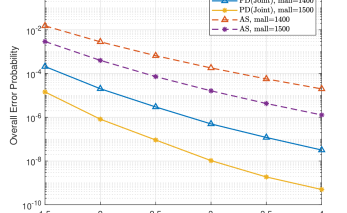
Figure 4: Overall error probability over total source power.

V-B Performance Evaluation

In this subsection, we analyze the system performance under diverse setups with respect to total power (constraint), total blocklength (constraint), packet size and so on. First, we study the influence of total source power on the system reliability. As shown in Fig. 4, higher total transmit power contributes to higher system FBL reliability, which is consistent with the discussion about Fig. 2. Moreover, all curves decrease steadily with virtually constant slopes. It indicates that although EH is a nonlinear process, the total amount of multiple transmit power has an approximately loglinear effect on the system reliability. To evaluate the performance enhancement of our proposed design, results based on a resource average sharing strategy, abbreviated as ‘AS’, are also provided. Through performance comparison, our proposed joint power and blocklength allocation design outperforms the AS and the reliability improvement progressively increases while the total source power increases from $31dBm$ to $36dBm$. In addition, when total blocklength increases from 1400 to 1500, both AS and PD achieve lower error probability and more interestingly, our PD can enlarge this system reliability enhancement, which indicates that the more resource is available in the system, the more flexible our PD is and the more sufficient resource utilization is achieved, thus the more potential is provided for reliability enhancement.

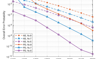
Figure 5: Overall error probability over WIT blocklength with different sensor number.

For the sake of a clearer description of the impact of blocklength on the system reliability, in Fig. 5 we depict the relationship between error and WIT blocklength under various sensor number. Clearly, the overall error probability monotonically decreases in the WIT blocklength, i.e., longer blocklength contributes to higher reliability. Moreover, in all cases (various sensor number and total blocklength), our PD outperforms the AS in terms of system reliability in an evident manner. More interestingly, this performance enhancement varies under diverse cases. For example, when the total blocklength ranges from 1500 to 2200, the performance enhancement boosts from two orders of magnitude to almost six orders while five sensors are deployed, i.e., longer blocklength contributes to more significant reliability enhancement. When the blocklength is 2100, the performance enhancement decreases from three orders of magnitude to two while sensor number enlarges from 5 to 9, which indicates that fewer sensors lead to relatively more significant reliability enhancement. The aforementioned phenomena can be explained by the fact that having fewer sensors or setting a longer blocklength likely provides additional flexibility in system design, resulting in a greater potential of the performance enhancement through the resource allocation. Specifically, the overall error probability is approximated as the cumulative sum of error probabilities of all short packet transmissions, i.e., a extremely poor transmission is highly likely to have a decisive impact on overall error probability bottleneck, resulting in very low system performance. To avoid such extreme situation, each sensor requires to be allocated sufficient blocklength for short packet transmission. Therefore larger total blockelngth or fewer sensors provides more room for system performance enhancement since blocklength with higher upper limit is available for per sensor, i.e., more room for blocklength optimization. In addition, curve ‘PD, N=9’ and curve ‘AS, N=5’ intersect at a point around blocklength 2100, which indicates that our PD can support more sensors’ short packet transmission compared with the AS in the same scenario with same system reliability requirements.

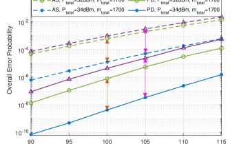
Figure 6: Overall error probability over packet size under nonlinear EH model.

Subsequently, we move on to study the relationship between the overall error probability and the packet size in Fig. 6. For the sake of analysis, we assume sensors transmit packets with same data amount. As the packet size increases, the overall error probability rises monotonically and the slope of each curve rarely changes. This indicates that the system can support large packet transmission but at the price of influencing the reliability, while such influence on reliability shows an approximate loglinear behavior in the packet size. In comparison to the AS benchmark, applying the PD introduces significant reliability improvements for the system under all circumstances. More interestingly, such error probability reductions are not constant. In particular, it is more significant in the small packet size region. Moreover, larger total source power or longer total blocklength contributes to lower error probability and such reliability enhancement introduced by PD is greater than the one by AS, which indicates that when additional resources are available in the system, our PD introduces more flexibility, i,e., a fuller and more efficient utilization of the resources is performed, thus magnifying the reliability enhancement with a given level of resource augmentation.

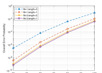
Figure 7: The impacts of the network topology on the overall error probability.

Our design is of significant generality that can be well adapted to networks with different topologies (including the distribution and number of nodes), based on which we explore the scalibility of our proposed algorithm and the impacts of topology on system reliability. Fig. 7 depicts the reliability performance when more sensors (70 to 100) are deployed for short packet transmissions, which indicates that our algorithm is of significant scalibility that can support massive number of sensors’ reliable transmission. As the sensor number increases, the FBL reliability decreases. On the one hand, the total error probability is the sum of transmission error probability of all sensors, which obviously increases with the number of sensors. On the other hand, considering the limited blocklength resource, more sensors represent fewer blocklength assigned per sensor. Moreover, as the number of sensors increases, the convergence speed (consumed time for optimization) will become relatively slower to some extent. The result indicates that the network has limited capability to support more sensors’ reliable short packet transmissions. Subsequently, we compare the performances under single-source and multi-source WPT networks and investigate the impacts of distributions of sensors on system reliability. In particular, we randomly deploy the sensors in square with certain length, and change the length of square. In comparison to the single-source case, multi-source WPT significantly improves the reliability even with the same total amount of WPT energy and WIT blocklength for consumption. More interestingly, for single-source case, when sensors are more dispersively distributed, i.e., ‘length’ increases from $1m$ to $3m$, less energy is harvested by certain sensors due to their further distances away from the source, which leads to a decrease in system reliability. Nevertheless, such reliability loss is extremely small in the multi-source case, which confirms a great advantage of multi-source WPT, i.e., the multi-source diversity introduces robustness to the reliability performance with respect to senors locations.

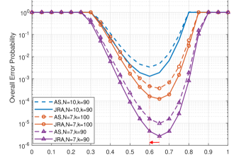
Figure 8: System reliability under diverse normalised WPT blocklength.

V-C Performance Advantages of the Joint Design

In this subsection, we illustrate the specific performance advantages of joint power and blocklength allocation design. Recall that as discussed in Section IV, there exists a tradeoff with respect to blocklength in the design, i.e., the compromise between the blocklength allocated for WPT and WIT phase along with the tradeoff inside the WIT phase (blocklength allocation among multi-sensors). To explore the blocklength allocation characteristics, Fig. 8 clearly depicts the system reliability versus diverse normalised WPT blocklength with the given total blocklength, where ‘JRA’ indicates the joint resource allocation. From Fig. 8, we learn that the overall error probability is quasi-convex with respect to the normalised WPT blocklength. In particular, the error probability first declines and gradually rises when the normalised WPT blocklength increases. When the normalised value varies by just 0.2 (from 0.65 to 0.85), the system reliability is weakened by more than four orders of magnitude (from $10^{-5}$ to $10^{-1}$), which indicates that reasonable blocklength allocation between two phases is significant for reliable transmission achievement. Moreover, for this given system ($N=7,k=90$), the optimal solution of blocklength allocated for WPT phase is higher than that for WIT phase, i.e., 65% of the total blocklength for WPT and 35% for WIT, which suggests that relatively more blocklength (time) should be allocated for EH, thus guaranteeing sufficient energy for short packet transmissions. More interestingly, the optimal value of normalised WPT blocklength decreases from 0.65 to 0.6 when more sensors are utilized (from 7 to 10). This may be explained by the fact that more sensors lead to a higher demand of blocklength for short packet transmisson, since each sensor has a minimum blocklength requirement to guarantee its reliable transmission based on (2), so that a high overall system reliability can be guaranteed. In addition, JRA obviously outperforms AS, and the overall error probability reduction generated by JRA becomes more significant as the packet size decreases (consistent with the results in Fig. 6) and the number of sensors increases. The results indicate that deploying more sensors actually introduces a higher diversity, i.e., providing more potentials for system performance enhancements.

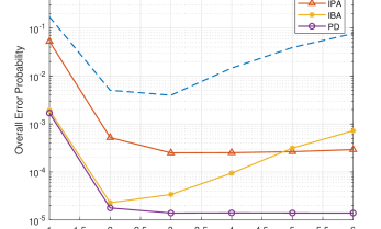
Figure 9: Joint optimization design vs. pure power allocation and pure blocklength allocations.

Finally, we explore the advantage of joint resource allocation design and investigate the respective contributions introduced by the power and the blocklength allocation to system reliability. As shown in Fig. 9, the results of independent power allocation (IPA), independent blocklength allocation (IBA), joint resource allocation (PD) and resource average sharing design (AS) are provided. We assume $\rm S_{2}$ and $\rm S_{3}$ are relatively closer to sensors while $\rm S_{4}$, $\rm S_{5}$ and $\rm S_{6}$ are relatively further away from sensors. In Fig. 9, we can observe that the joint power and blocklength allocation design significantly outperforms the ‘AS’,‘IPA’,‘IBA’ and the performance enhancement enlarges as the source number increases (compared with ‘AS’ and ‘IBA’). More interestingly, both curve ‘AS’ and ‘IBA’ first decrease and subsequently increase as the source number increases. It can be interpreted by the fact that the new added WPT source $\rm S_{4}$, $\rm S_{5}$ and $\rm S_{6}$ have relatively weaker LoS to sensors compared with $\rm S_{2}$ and $\rm S_{3}$. Under total power limitation, power average sharing strategy will diminish the advantage of sources with higher WPT capability and consequently reduce the system FBL reliability. By contrast, ‘IPA’ and ‘PD’ (including power allocation) can achieve better reliability performance when more sources ($M\geq 5$) are deployed for WPT. Moreover, it can be observed that when $M=1$, the result of ‘IBA’ coincides with that of PD, since the single source takes up the entire power resource without power allocation, i.e., ‘PD’ is equivalent to the ‘IBA’. Nevertheless, as the number of WPT sources increases, the reliability advantage of ‘PD’ is gradually revealed. Besides, by comparing ‘IPA’ and ‘IBA’, we can learn that ‘IBA’ significantly outperforms ‘IPA’ when $M\leq 4$, while ‘IPA’ achieves higher reliability when $M\geq 5$. The results suggest that in scenarios where power and blocklength are not allowed to be joint optimized simultaneously, pure power allocation is more proffered for a scenario with more WPT sources, while spending overhead to achieve an efficient blocklength allocation pays off more when the network has less WPT sources.

VI Conclusion

In this work, we considered a multi-source WPT enabled multi-sensor communication network, where sensors are activated by the nonlinear EH process and transmit short packets via FBL codes. For the first time, we characterized the relationship among FBL reliability, multiple source power, WPT blocklength as well as multiple WIT blocklengths for such network. With a total source power limitation, we considered a power allocation design aiming at minimizing the overall error probability under fixed frame structure. Subsequently, the design was extended to dynamic frame structure, in which a joint resource allocation design was provided via jointly optimizing multiple source power and blocklengths under total power and blocklength constraints. To solve the challenging non-convex optimization problems, novel variable substitution and SCA algorithm are exploited to reformulate the optimization problems. Based on the iterative algorithm, an efficient sub-optimal solution was thus achieved. Via numerical simulations, we have demonstrated significant advantages of our proposed design and confirmed the importance of the deployment of multiple WPT sources and nonlinear EH model. Simulation results also provided guidelines for practical system designs.

At last, we finalize this work by spotlighting its high extensibility. The methodology of the proposed resource allocation design minimizing overall error probability (including the way addressing the tradeoff among multiple WPT sources) can be extended to designs for multi-source WPT enabled communications, e.g., energy-efficiency maximization, end-to-end latency minimization, location planning for multi WPT sources, and so on. Moreover, the proposed methods for non-convex problem settlement, including variable substitutions, complex relationship decoupling, auxiliary variables introduction, can be applied to facilitate other optimizations of non-convex problems, especially for scenarios with coupled resource supply and consumption.

References

- [1]
- [2] N. Guo, X. Yuan, Y. Hu, F. Chong and A. Schmeink, “Reliability-oriented resource allocation for multi-source WPT enabled multi-user short packet communications,” in IEEE ISWCS, Oct. 2022, Hangzhou, China.
- [3] F. Guo, F. R. Yu, H. Zhang, X. Li, H. Ji and V. C. M. Leung, “Enabling massive IoT toward 6G: a comprehensive survey,” IEEE Internet Things J., vol. 8, no. 15, pp. 11891-11915, 1 Aug.1, 2021.
- [4] X. Wang, A. Ashikhmin and X. Wang, “Wirelessly powered cell-free IoT: analysis and optimization,” IEEE Internet Things J., vol. 7, no. 9, pp. 8384-8396, Sept. 2020.
- [5] R. Morsi, D. S. Michalopoulos, and R. Schober, “Performance analysis of near-optimal energy buffer aided wireless powered communication,” IEEE Trans. Wireless Commun., vol. 17, no. 2, pp. 863–881, Feb. 2018.
- [6] Z. Zhang, H. Pang, A. Georgiadis and C. Cecati, “Wireless power transfer — an overview,” IEEE Trans. Ind. Electron., vol. 66, no. 2, pp. 1044-1058, Feb. 2019.
- [7] M. Xiong, X. Wei, Y. Huang, Z. Luo, and H. Dai, “Research on novel flexible high-saturation nanocrystalline cores for wireless charging systems of electric vehicles,” IEEE Trans. Ind. Electron., vol. 68, no. 9, pp. 8310–8320, Sep. 2021.
- [8] A. Buffi, A. Michel, P. Nepa and G.Manara, “Numerical analysis of wireless power transfer in near-field UHF-RFID systems,” in Wireless Power Transfer, vol. 5, no. 1, pp. 42-53, Mar. 2018.
- [9] N. u. Hassan, S. -W. Hong and B. Lee, “A Robust Multioutput Self-Regulated Rectifier for Wirelessly Powered Biomedical Applications,” IEEE Trans. Ind. Electron., vol. 68, no. 6, pp. 5466-5472, Jun. 2021.
- [10] Y. Sun et al., “Recycling Wasted Energy for Mobile Charging,” in 2021 IEEE 29th International Conference on Network Protocols (ICNP), Dallas, TX, USA, 2021.
- [11] X. Hou, Z. Wang, Y. Su, Z. Liu, Z. Deng, “A Dual-Frequency Dual-Load Multirelay Magnetic Coupling Wireless Power Transfer System Using Shared Power Channel,” IEEE Trans. Power Electron., vol. 37, no. 12, pp. 15717-27, Dec. 2022.
- [12] Y. Zhu, Y. Liu, J. Zhao, M. Li and Q. Wu, “Joint time allocation and beamforming design for IRS-aided coexistent cellular and sensor networks,” 2021 IEEE Global Communications Conference (GLOBECOM), Dec. 2021, Madrid, Spain.
- [13] F. Zhou, Y. Wu, R. Q. Hu and Y. Qian, “Computation rate maximization in UAV-enabled wireless-powered mobile-edge computing systems,” IEEE J. Sel. Areas Commun., vol. 36, no. 9, pp. 1927-1941, Sept. 2018.
- [14] R. Malik and M. Vu, “Energy-efficient joint wireless charging and computation offloading in MEC systems,” IEEE J. Sel. Top. Signal. Process, vol. 15, no. 5, pp. 1110-1126, Aug. 2021.
- [15] B. Li, F. Si, W. Zhao and H. Zhang, “Wireless powered mobile edge computing with NOMA and user cooperation,” IEEE Trans. Veh. Technol., vol. 70, no. 2, pp. 1957-1961, Feb. 2021.
- [16] X. Yuan, H. Jiang, Y. Hu, A. Schmeink, “Joint analog beamforming and trajectory planning for energy-efficient UAV-enabled nonlinear wireless power transfer,” IEEE J. Sel. Areas Commun., vol. 40, no. 10, pp. 2914-29, Oct. 2022.
- [17] Y. Hu, X. Yuan, G. Zhang and A. Schmeink, “Sustainable wireless sensor networks with UAV-enabled wireless power transfer,” IEEE Trans. Veh. Technol., vol. 70, no. 8, pp. 8050-8064, Aug. 2021.
- [18] J. Zheng, J. Zhang and B. Ai, “UAV communications with WPT-aided cell-free massive MIMO systems,” IEEE J. Sel. Areas Commun., vol. 39, no. 10, pp. 3114-3128, Oct. 2021.
- [19] N. Shanin, L. Cottatellucci and R. Schober, “Optimal transmit strategy for multi-user MIMO WPT systems With non-Linear energy harvesters,” IEEE Trans. Commun., vol. 70, no. 3, pp. 1726-1741, Mar. 2022.
- [20] Y. Zhu, L. Wang, K. -K. Wong, S. Jin and Z. Zheng, “Wireless power transfer in massive MIMO-aided HetNets with user association,” IEEE Trans. Commun., vol. 64, no. 10, pp. 4181-4195, Oct. 2016.
- [21] G. N. Kamga and S. Aïssa, “Wireless power transfer in mmWave massive MIMO systems with/without rain attenuation,” IEEE Trans. Commun., vol. 67, no. 1, pp. 176-189, Jan. 2019.
- [22] O. Waqar and R. Adve, “On the throughput of wireless powered communication systems with a multiple antenna bidirectional relay,” IEEE Wireless Commun. Lett., vol. 8, no. 3, pp. 941-944, Jun. 2019.
- [23] Z. Chang, Z. Wang, X. Guo, Z. Han and T. Ristaniemi, “Energy-efficient resource allocation for wireless powered massive MIMO system with imperfect CSI,” IEEE Trans. Green Commun. and Netw. vol. 1, no. 2, pp. 121-130, Jun. 2017.
- [24] Y. Wu, Y. Song, T. Wang, L. Qian and T. Q. S. Quek, “Non-orthogonal multiple access assisted federated learning via wireless power transfer: a cost-efficient approach,” IEEE Trans. Commun., vol. 70, no. 4, pp. 2853-2869, Apr. 2022.
- [25] X. Yuan, Y. Hu, J. Gross and A. Schmeink, “Simultaneous wireless information and power transfer in low-latency relaying networks with nonlinear energy harvesting,” in IEEE Statistical Signal Processing Workshop (SSP), pp. 281-285, Rio de Janeiro, Brazil, Jul. 2021.
- [26] N. Guo, X. Yuan, Y. Hu and A. Schmeink, “SWIPT-enabled multi-user cooperative communication with nonlinear energy harvesting,” in 25th International ITG Workshop on Smart Antennas, French Riviera, France, Nov. 2021.
- [27] Q. Wu, M. Tao, D.W. Kwan Ng, W. Chen, R. Schober, “Energy-efficient resource allocation for wireless powered communication networks,” IEEE Trans. Wirel. Commun., vol. 15, no. 3, pp. 2312-27, Mar. 2016.
- [28] Z. Feng, B. Clerckx, Y. Zhao, “Waveform and beamforming design for intelligent reflecting surface aided wireless power transfer: single-user and multi-user solutions,” IEEE Trans. Wirel. Commun., vol. 21, no. 7, pp. 5346-5361, Jul. 2022.
- [29] J. -M. Kang, I. -M. Kim and D. I. Kim, “Wireless information and power transfer: rate-energy tradeoff for nonlinear energy harvesting,” IEEE Trans. Wirel. Commun., vol. 17, no. 3, pp. 1966-1981, Mar. 2018.
- [30] D. Xu, V. Jamali, X. Yu, D. W. K. Ng and R. Schober, “Optimal resource allocation design for large IRS-assisted SWIPT systems: a scalable optimization framework,” IEEE Trans. Commun., vol. 70, no. 2, pp. 1423-1441, Feb. 2022.
- [31] Q. Wu and R. Zhang, “Weighted sum power maximization for intelligent reflecting surface aided SWIPT,” IEEE Wireless Commun. Lett., vol. 9, no. 5, pp. 586-590, May 2020.
- [32] T. Arakawa, S. Goguri, J. V. Krogmeier et al., “Optimizing wireless power transfer from multiple transmit coils,” IEEE Access, vol. 6, pp. 23828-23838, 2018.
- [33] Y. Ye, L. Shi, X. Chu, G. Lu and S. Sun, “Mutualistic Cooperative Ambient Backscatter Communications Under Hardware Impairments,” in IEEE Transactions on Communications, vol. 70, no. 11, pp. 76 56-7668, Nov. 2022.
- [34] S. Abeywickrama, R. Zhang and C. Yuen, “Refined Nonlinear Rectenna Modeling and Optimal Waveform Design for Multi-User Multi-Antenna Wireless Power Transfer,” in IEEE J. Sel. Topics Signal Process., vol. 15, no. 5, pp. 1198-1210, Aug. 2021.
- [35] X. Yuan, Y. Hu, and A. Schmeink, “Joint design of UAV trajectory and directional antenna orientation in UAV-enabled wireless power transfer networks,” in IEEE J. Sel. Areas Commun., vol. 39, no. 10, pp. 3081–3096, Oct. 2021.
- [36] H. Lang, A. Ludwig and C. D. Sarris, “Convex optimization of wireless power transfer systems with multiple transmitters,” IEEE Trans. Antennas Propag., vol. 62, no. 9, pp. 4623-4636, Sept. 2014.
- [37] R. Hamdi, M. Chen, A. B. Said, M. Qaraqe and H. V. Poor, “Federated learning over energy harvesting wireless networks,” IEEE Internet Things J., vol. 9, no. 1, pp. 92-103, 1 Jan. 2022.
- [38] X. Yuan, Y. Hu, R. Schober and A. Schmeink, “Convexity analysis of nonlinear wireless power transfer with multiple RF sources,” IEEE Trans. Veh. Technol., vol. 71, no. 10, pp. 11311-11316, Oct. 2022.
- [39] Y. Polyanskiy, H. V. Poor and S. Verdu, “Channel coding rate in the finite blocklength regime,” IEEE Trans. Inf. Theory., vol. 56, no. 5, pp. 2307-2359, May 2010.
- [40] C. She, C. Yang and T. Q. S. Quek, “Cross-layer optimization for ultra-reliable and low-Latency radio access networks,” in IEEE Trans. Wirel. Commun., vol. 17, no. 1, pp. 127-141, Jan. 2018.
- [41] E. Boshkovska, D. W. K. Ng, N. Zlatanov and R. Schober, “Practical Non-Linear Energy Harvesting Model and Resource Allocation for SWIPT Systems,” in IEEE Commun. Lett., vol. 19, no. 12, pp. 2082-2085, Dec. 2015.
- [42] L. Shi, Y. Ye, R. Q. Hu and H. Zhang, “Energy Efficiency Maximization for SWIPT Enabled Two-Way DF Relaying,” in IEEE Signal Processing Lett., vol. 26, no. 5, pp. 755-759, May 2019.
- [43] Y. Hu, X. Yuan, T. Yang, B. Clerckx, and A. Schmeink, “On the convex properties of wireless power transfer with nonlinear energy harvesting,” IEEE Trans. Veh. Technol., vol. 69, no. 5, pp. 5672-5676, May. 2020.
- [44] Y. Hu, Y. Zhu, M. C. Gursoy and A. Schmeink, “SWIPT-enabled relaying in IoT networks operating with finite blocklength codes,” IEEE J. Sel. Areas Commun., vol. 37, no. 1, pp. 74-88, Jan. 2019.
- [45] Y. Zhu, Y. Hu, X. Yuan, M. C. Gursoy, H. V. Poor, A. Schmeink, ”Joint convexity of error probability in blocklength and transmit power in the finite blocklength regime,” IEEE Trans. Wirel. Commun., Sep. 2022.
- [46] B. Clerckx and E. Bayguzina, ”Waveform Design for Wireless Power Transfer,” in IEEE Trans. Signal Process., vol. 64, no. 23, pp. 6313-6328, 1 Dec.1, 2016.