Atmospheric turbulence does not change the degree of polarization of vector beams

Abstract

We propose a novel theoretical framework to demonstrate vector beams whose degree of polarization does not change on atmospheric propagation. Inspired by the Fresnel equations, we derive the reflective and refractive field of vector beams propagating through a phase screen by employing the continuity of electromagnetic field. We generalize the conventional split-step beam propagation method by considering the vectorial properties in the vacuum diffraction and the refractive properties of a single phase screen. Based on this vectorial propagation model, we extensively calculate the change of degree of polarization (DOP) of vector beams under different beam parameters and turbulence parameters both in free-space and satellite-mediated links. Our result is that whatever in the free-space or satellite-mediated regime, the change of DOP mainly fluctuates around the order of $10^{-13}$ to $10^{-6}$, which is almost negligible.

1 Introduction

One of the essential properties of light, such as polarization, was proven to be a paramount resource in many cutting-edge experiments[1, 2, 3, 4, 5, 6, 7], which offers a proper way to understand the real physical world and remains to be the theme of much fundamental research today. The historical survey of understanding the polarization can be dated back to the underlying theory, bearing Stock’s name, in 1852[8]. It leads to a straightforward description of degree of polarization (DOP)[9, 10, 11, 12] and provides an elegant geometrical picture to analyze the impacts of polarization transformations[13]. However, such theory cannot describe the random nature of the light emission process. For this reason, Wolf presents a statistical framework which bridges the connection between coherence and polarization of random electromagnetic beams[14, 15, 16, 17].

The question of whether beams whose DOP changes on propagation also arises on the basis of the recent theory formulated in terms of the cross-spectral density matrix[18, 19, 20, 21, 22]. Over past decades, it has been known that DOP can keep unchanged on propagation, including free-space channel[23, 24, 25, 26, 27, 28, 29, 30, 31, 32] or turbulent channel[33, 34, 35, 36, 37], but it commonly needs to satisfy some specific conditions. Especially, to investigate the effects of atmospheric turbulence on DOP, many researchers have focused their efforts primarily on how to introduce a random phase into the cross-spectral density matrix by introducing the extended Huygens Fresnel principle[33, 34, 35, 36, 37]. In summary, all of the aforementioned conclusions are obtained through the coherence theory of light.

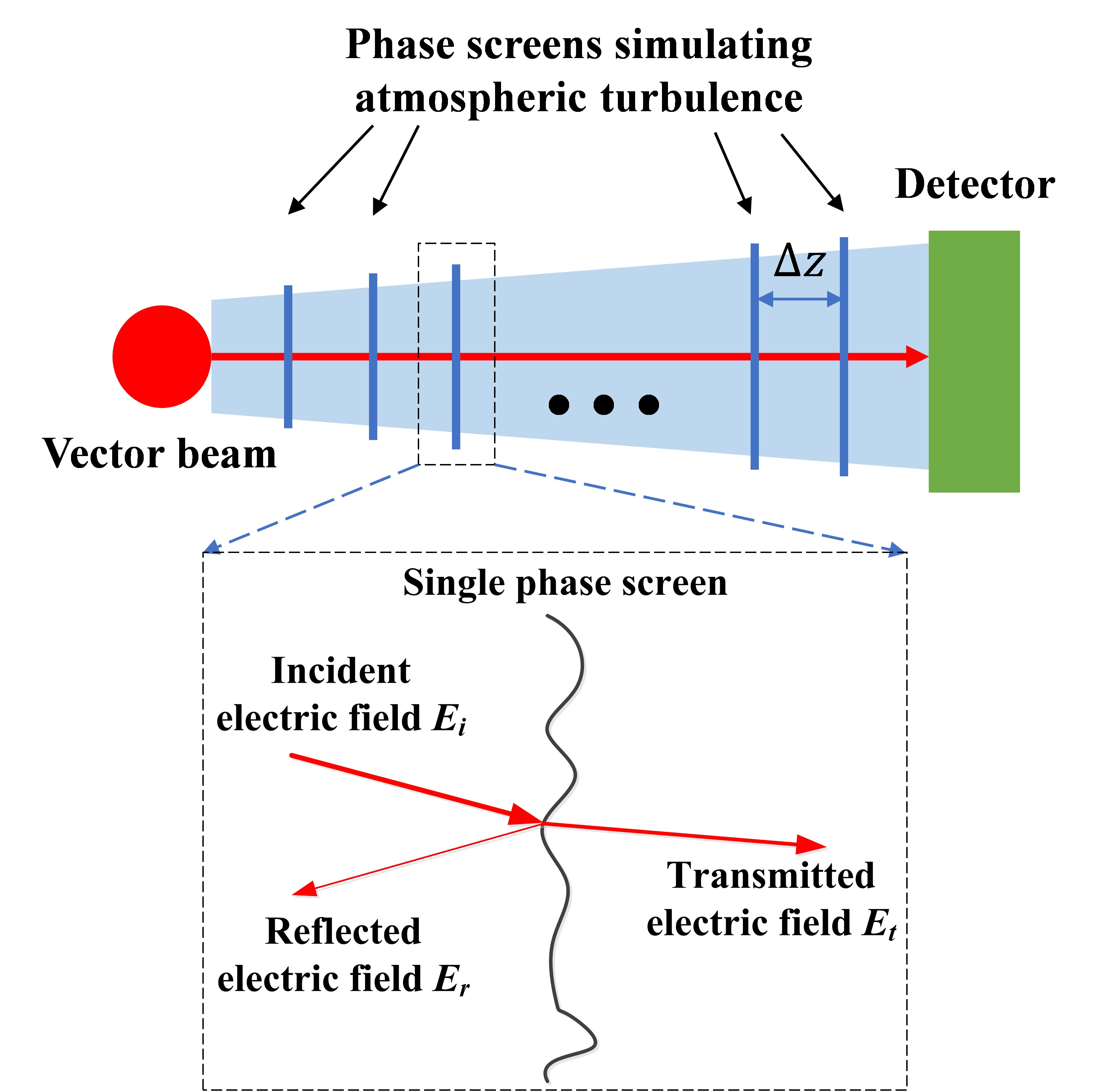
Figure 1: The source generates a single vector beam and sends it through a turbulent atmosphere toward a detector. A turbulent channel is divided into multiple turbulent cells, each cell introduces a random contribution $\varphi$ to the phase, and the effects of reflection and refraction to the vector beam. The process of vector beams propagating between two cells is built by the vectorial diffraction theory. The phase screen array is ladder-shaped distributed because the divergence angle becomes larger as propagation distance increases.

In this article, we propose a novel theoretical framework to demonstrate vector beams whose DOP does not change on atmospheric propagation, which is based on the continuity of electromagnetic field[38, 39] instead of employing the cross-spectral density matrix. The main difference between our method and others is that we suggest that light propagation through a random phase screen is the process of reflection and refraction. Concretly, we believe that one of the polarized components of light wave falls on to a boundary between two homogeneous media of different optical properties, it will be split into two orthogonally polarized components: a component possess the same polarization with the incident light and another is orthogonal to the incident one[40]. After undergoing the modulation of a series of turbulent cells, it might change the DOP of the incident vector beam.

2 Theory

The conceptual diagram of a vector beam propagating through turbulence that is depicted by our theoretical model is given in Fig. 1. Since a turbulent channel can be regarded as a series of equally spaced turbulent cells, the effects of turbulence on propagation can be splitted into several iterations of the same modulation. Now, let us begin by recalling the description scheme of the effects of atmospheric turbulence on scalar beam in general referring to the split-step beam propagation method[41]. It means that each cell introduces a random contribution $\varphi$ to the phase, but essentially there is no change in the amplitude; besides, intensity fluctuations build up by diffraction over many cells. It should be noted that, to agree well with the phase structure function of the Kolmogorov turbulence model, random phase screen lost low spatial frequencies need to be compensated using the subharmonic method[42].

It is worth highlighting that the conventional theoretical framework of atmospheric propagation is an incomplete characterization for vector beams, whereas whether the DOP of beams changes also needs to be investigated within this method. Moreover, the split-step method will lose its usefulness when studying the influence of turbulence on a vector beam. Hence, we further adopt the wave refraction and vectorial diffraction theory[43, 44] together to construct the atmospheric propagation model for a general polarized vector beam. Without loss of generality, we summarize and divide the procedure of this model into two steps as follows: Firstly, we decompose the electric field of a general vector beam into horizontal and vertical components. Secondly, for each component of the electric field, the modulation by the random phase and refraction function of the phase screen and the subsequent diffraction together is repeated several times in the simulation process. The crucial procedure in the above model that leading to a change in the DOP of electric field is the several refractions of multiple phase screen.

To quantify the adverse impact of phase screen on DOP, we report the refraction of a single random phase screen for the incident electric field $\mathbf{E}\left(x,y\right)$ of wave vector $\mathbf{k}$. We assume that $E_{x}\left(x,y\right)$ and $E_{y}\left(x,y\right)$ represent the horizontal and vertical components of $\mathbf{E}\left(x,y\right)$. The relationship between $\mathbf{k}$ and $\phi\left(x,y\right)$ obeys

$$\mathbf{k}=\nabla\phi\left(x,y\right)$$ (1)

with $\phi\left(x,y\right)$ denoting the phase of one components of $\mathbf{E}\left(x,y\right)$ (i.e., $E_{x}\left(x,y\right)$ or $E_{y}\left(x,y\right)$), or more explicitly, $\mathbf{k}=\left(\phi_{x},\phi_{y},k_{z}\right)$, where $k_{z}^{2}=\left|\mathbf{k}\right|^{2}-\phi_{x}^{2}-\phi_{y}^{2}$. As shown in Fig. 1, if we suppose the postive direction of $z$ as the propagation direction, Eq. (1) can be further re-evaluated in terms of incident, transmitted and reflected components as follows

$$\mathbf{k}^{\left(i\right)} = \left(\phi_{x}^{\left(i\right)},\phi_{y}^{\left(i\right)},\sqrt{\left(2\pi n_{i}/\lambda\right)^{2}-\phi_{x}^{\left(i\right)2}-\phi_{y}^{\left(i\right)2}}\right)$$

$$\mathbf{k}^{\left(r\right)} = \left(\phi_{x}^{\left(r\right)},\phi_{y}^{\left(r\right)},-\sqrt{\left(2\pi n_{r}/\lambda\right)^{2}-\phi_{x}^{\left(r\right)2}-\phi_{y}^{\left(r\right)2}}\right)$$ (2)

$$\mathbf{k}^{\left(t\right)} = \left(\phi_{x}^{\left(t\right)},\phi_{y}^{\left(t\right)},\sqrt{\left(2\pi n_{t}/\lambda\right)^{2}-\phi_{x}^{\left(t\right)2}-\phi_{y}^{\left(t\right)2}}\right)$$

with the subscripts $i$, $r$, $t$ referring to incident, transmitted and reflected components, respectively, where $\phi_{x}^{\left(l\right)}$ and $\phi_{y}^{\left(l\right)}$ ($l=i,r,t$) represent the partial derivative of one components of $\mathbf{E}^{\left(l\right)}\left(x,y\right)$ ($l=i,r,t$) in $x$ and $y$ directions, $n_{l}$ ($l=i,r,t$) denotes the refractive index of two homogeneous media and $\lambda$ is wavelength. By means of the orthogonal formula $\mathbf{E}^{\left(l\right)}\left(x,y\right)\cdot\mathbf{k}^{\left(l\right)}=0$ ($l=i,r,t$), we can express the incident, transmitted and reflected components of $\mathbf{E}\left(x,y\right)$ as

$$\mathbf{E}^{\left(i\right)} = \left(E_{x}^{\left(i\right)},E_{y}^{\left(i\right)},-\left(E_{x}^{\left(i\right)}k_{x}^{\left(i\right)}+E_{y}^{\left(i\right)}k_{y}^{\left(i\right)}\right)/k_{z}^{\left(i\right)}\right)$$

$$\mathbf{E}^{\left(r\right)} = \left(E_{x}^{\left(r\right)},E_{y}^{\left(r\right)},\left(E_{x}^{\left(r\right)}k_{x}^{\left(r\right)}+E_{y}^{\left(r\right)}k_{y}^{\left(r\right)}\right)/k_{z}^{\left(r\right)}\right)$$ (3)

$$\mathbf{E}^{\left(t\right)} = \left(E_{x}^{\left(t\right)},E_{y}^{\left(t\right)},\left(E_{x}^{\left(t\right)}k_{x}^{\left(t\right)}+E_{y}^{\left(t\right)}k_{y}^{\left(t\right)}\right)/k_{z}^{\left(t\right)}\right)$$

where $k_{x}^{\left(l\right)}=\phi_{x}^{\left(l\right)}$, $k_{y}^{\left(l\right)}=\phi_{y}^{\left(l\right)}$ and $k_{z}^{\left(l\right)}=\sqrt{\left(2\pi n_{l}/\lambda\right)^{2}-\phi_{x}^{\left(l\right)2}-\phi_{y}^{\left(l\right)2}}$ ($l=i,r,t$). Other than that, the components of magnectic field are obtained by combining the ralation $\mathbf{H=}n\frac{\mathbf{k}}{\left|\mathbf{k}\right|}\times\mathbf{E}$ and Eq. (3), we gives

$$\mathbf{H}^{\left(i\right)} = \frac{n_{i}}{\left|\mathbf{k}^{\left(i\right)}\right|k_{z}^{\left(i\right)}}\left(\begin{array}[]{c}-\left[E_{x}^{\left(i\right)}k_{x}^{\left(i\right)}k_{y}^{\left(i\right)}+E_{y}^{\left(i\right)}\left(\left|\mathbf{k}^{\left(i\right)}\right|^{2}-k_{x}^{\left(i\right)2}\right)\right]\\ E_{y}^{\left(i\right)}k_{x}^{\left(i\right)}k_{y}^{\left(i\right)}+E_{x}^{\left(i\right)}\left(\left|\mathbf{k}^{\left(i\right)}\right|^{2}-k_{y}^{\left(i\right)2}\right)\\ \left(E_{y}^{\left(i\right)}k_{x}^{\left(i\right)}-E_{x}^{\left(i\right)}k_{y}^{\left(i\right)}\right)k_{z}^{\left(i\right)}\end{array}\right)$$ (7)

$$\mathbf{H}^{\left(r\right)} = \frac{n_{r}}{\left|\mathbf{k}^{\left(r\right)}\right|k_{z}^{\left(r\right)}}\left(\begin{array}[]{c}E_{x}^{\left(r\right)}k_{x}^{\left(r\right)}k_{y}^{\left(r\right)}+E_{y}^{\left(r\right)}\left(\left|\mathbf{k}^{\left(r\right)}\right|^{2}-k_{x}^{\left(r\right)2}\right)\\ -\left[E_{y}^{\left(r\right)}k_{x}^{\left(r\right)}k_{y}^{\left(r\right)}+E_{x}^{\left(r\right)}\left(\left|\mathbf{k}^{\left(r\right)}\right|^{2}-k_{y}^{\left(r\right)2}\right)\right]\\ \left(E_{y}^{\left(r\right)}k_{x}^{\left(r\right)}-E_{x}^{\left(r\right)}k_{y}^{\left(r\right)}\right)k_{z}^{\left(r\right)}\end{array}\right)$$ (11)

$$\mathbf{H}^{\left(t\right)} = \frac{n_{t}}{\left|\mathbf{k}^{\left(t\right)}\right|k_{z}^{\left(t\right)}}\left(\begin{array}[]{c}-\left[E_{x}^{\left(t\right)}k_{x}^{\left(t\right)}k_{y}^{\left(t\right)}+E_{y}^{\left(t\right)}\left(\left|\mathbf{k}^{\left(t\right)}\right|^{2}-k_{x}^{\left(t\right)2}\right)\right]\\ E_{y}^{\left(t\right)}k_{x}^{\left(t\right)}k_{y}^{\left(t\right)}+E_{x}^{\left(t\right)}\left(\left|\mathbf{k}^{\left(t\right)}\right|^{2}-k_{y}^{\left(t\right)2}\right)\\ \left(E_{y}^{\left(t\right)}k_{x}^{\left(t\right)}-E_{x}^{\left(t\right)}k_{y}^{\left(t\right)}\right)k_{z}^{\left(t\right)}\end{array}\right)$$ (15)

It is well-known that boundary conditions of electromagnetic field demand that across the boundary the tangential components of $\mathbf{E}$ and $\mathbf{H}$ should be continuous, namely[38, 39]

$$E_{x}^{\left(i\right)}+E_{x}^{\left(r\right)} = E_{x}^{\left(t\right)},E_{y}^{\left(i\right)}+E_{y}^{\left(r\right)}=E_{y}^{\left(t\right)}$$

$$H_{x}^{\left(i\right)}+H_{x}^{\left(r\right)} = H_{x}^{\left(t\right)},H_{y}^{\left(i\right)}+H_{y}^{\left(r\right)}=H_{y}^{\left(t\right)}$$ (16)

Hence, substituting Eq. (3) and Eq. (11) into Eq. (16) and undergoing a series of algebraic operations, we can immediately calculate the relationship between $E_{m}^{\left(i\right)}$ and $E_{m}^{\left(t\right)}$ ($m=x,y$)

$$E_{x}^{\left(t\right)} = \frac{M_{12}M_{23}-M_{13}M_{22}}{M_{11}M_{22}-M_{12}M_{21}}$$

$$E_{y}^{\left(t\right)} = \frac{M_{13}M_{21}-M_{11}M_{23}}{M_{11}M_{22}-M_{12}M_{21}}$$ (17)

where

$$M_{11}=M_{22}=\frac{n_{i}}{\left|\mathbf{k}^{\left(i\right)}\right|k_{z}^{\left(i\right)}}k_{x}^{\left(i\right)}k_{y}^{\left(i\right)}+\frac{n_{t}}{\left|\mathbf{k}^{\left(t\right)}\right|k_{z}^{\left(t\right)}}k_{x}^{\left(t\right)}k_{y}^{\left(t\right)}$$ (18)

$$M_{12}=F\left(k_{x}^{\left(i\right)},k_{x}^{\left(t\right)}\right),M_{21}=F\left(k_{y}^{\left(i\right)},k_{y}^{\left(t\right)}\right)$$ (19)

$$M_{13}=-2\frac{n_{i}}{\left|\mathbf{k}^{\left(i\right)}\right|k_{z}^{\left(i\right)}}\left[E_{x}^{\left(i\right)}k_{x}^{\left(i\right)}k_{y}^{\left(i\right)}+E_{y}^{\left(i\right)}\left(\left|\mathbf{k}^{\left(i\right)}\right|^{2}-k_{x}^{\left(i\right)2}\right)\right]$$ (20)

$$M_{23}=-2\frac{n_{i}}{\left|\mathbf{k}^{\left(i\right)}\right|k_{z}^{\left(i\right)}}\left[E_{y}^{\left(i\right)}k_{x}^{\left(i\right)}k_{y}^{\left(i\right)}+E_{x}^{\left(i\right)}\left(\left|\mathbf{k}^{\left(i\right)}\right|^{2}-k_{y}^{\left(i\right)2}\right)\right]$$ (21)

with

$$F\left(k_{1},k_{2}\right)=\frac{n_{i}}{\left|\mathbf{k}^{\left(i\right)}\right|k_{z}^{\left(i\right)}}\left(\left|\mathbf{k}^{\left(i\right)}\right|^{2}-k_{1}^{2}\right)+\frac{n_{t}}{\left|\mathbf{k}^{\left(t\right)}\right|k_{z}^{\left(t\right)}}\left(\left|\mathbf{k}^{\left(t\right)}\right|^{2}-k_{2}^{2}\right)$$ (22)

So far, we have quantified the change in the electric field of $\mathbf{E}^{\left(i\right)}$ after refraction through the phase screen, which is the key step to determine whether DOP changes after the electric field is propagated through turbulence. It should be stressed that when analyzing the DOP of any component of the vector light, either $E_{x}^{\left(i\right)}$ or $E_{y}^{\left(i\right)}$ of the electric field needs to be set to zero. Therefore, we can see from Eq. (17) that even if the incident light is polarized in a single direction, the propagated light refracted by a phase screen still has two $x$, $y$ directional polarization components. More generally, the result of such a modulation is that the $x$ ($y$) component of the output light is in fact a mixture of the $x$ ($y$) component produced by the refraction of the $x$ and $y$ direction components of the incident light through a random phase screen. Finally, we also should point out that in our theoretical calculations, the fact that DOP does not change because of diffraction is taken for granted since DOP hardly varies with the diffraction distance if the various parameters satisfy the appropriate conditions.

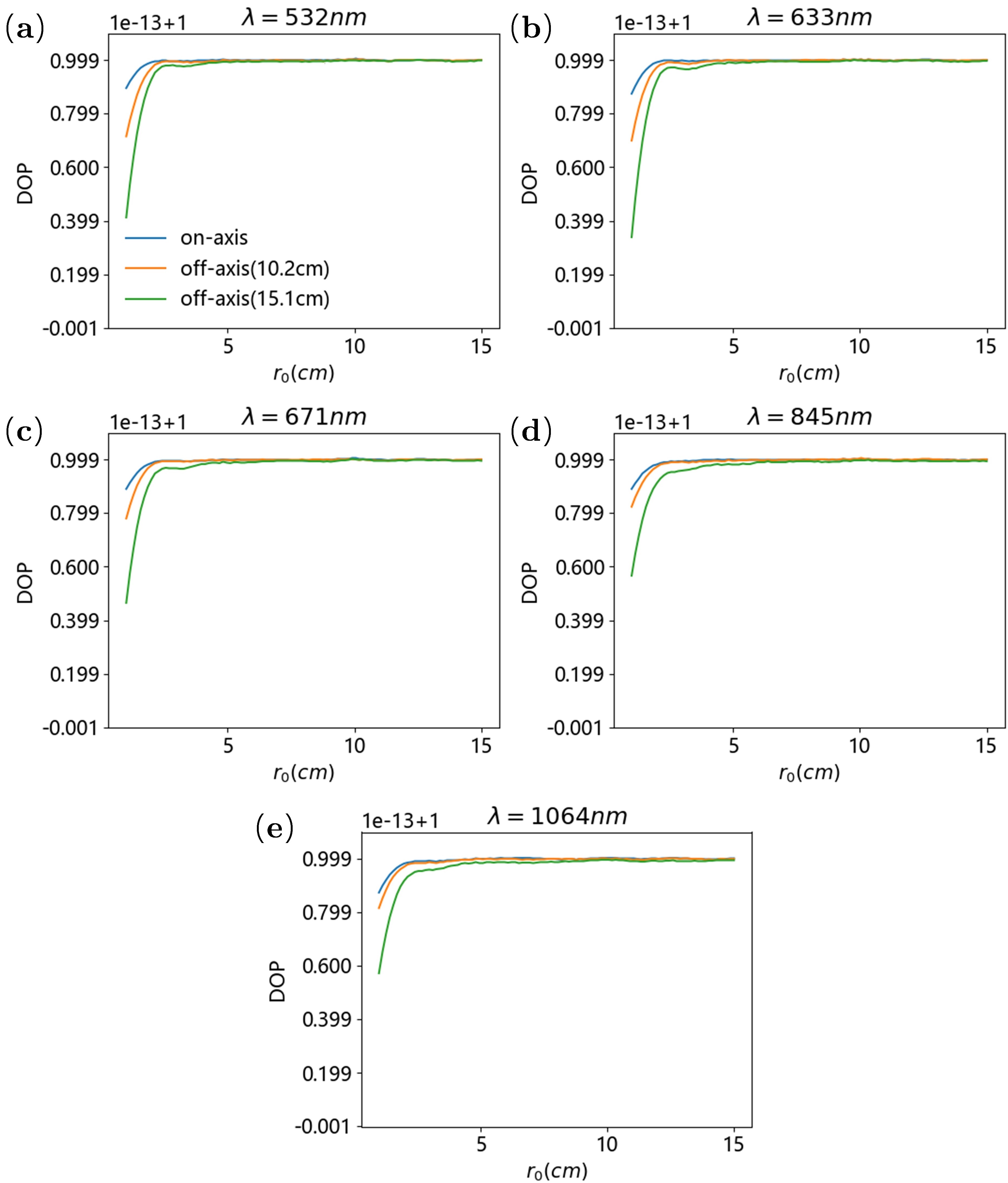
Figure 2: DOP of a circularly polarized light as a function of $r_{0}$ for different values of wavelength: (a) $\lambda=532nm$; (b) $\lambda=633nm$; (c) $\lambda=671nm$; (d) $\lambda=845nm$; (e) $\lambda=1064nm$. All curves in each plot correspond to the DOP calculated under different off-axis magnitudes.

3 Results

3.1 Free-space links

Fig. 2 illustrates how the DOP of circularly polarized light changes with respect to the atmospheric coherence length $r_{0}$ under different off-axis magnitudes, where each plot from upper to bottom represents the results of different values of wavelength (In the simulation of free-space atmospheric propagation, we adopt the side length at source plane and receiver plane of $30cm$ with a spatial resolution of $1.2mm$ and calculate the DOP averaged over $1000$ realizations of turbulence). It can be seen that in the strong turbulence regime, the DOP of circularly polarized light rapidly decreases with the increase of turbulence strength, whereas in the weak-to-moderate turbulence regime, DOP almost does not change as $r_{0}$ gradually decreases. We found that, overall, the change of DOP affected by atmospheric turbulence mainly fluctuates around the order of $10^{-13}$, which can be almost ignored. Moreover, we observe that the polarization properties of the optical field offset from the center of the optical axis are strongly affected by turbulence. In other words, atmospheric turbulence has smaller effect on the DOP of on-axis optical field compared to that of off-axis one, which leads to a reduction of DOP as the off-axis magnitude becomes larger. Finally, from the comparison between Fig. 2(a) to 2(e), we see that the DOP at the center of the optical axis hardly varies with the wavelength, yet the polarization properties of the off-axis optical field may become smaller as the wavelength increases, which is mainly caused by the fact that a short wavelength polarized light undergoes a larger effect of atmospheric turbulence.

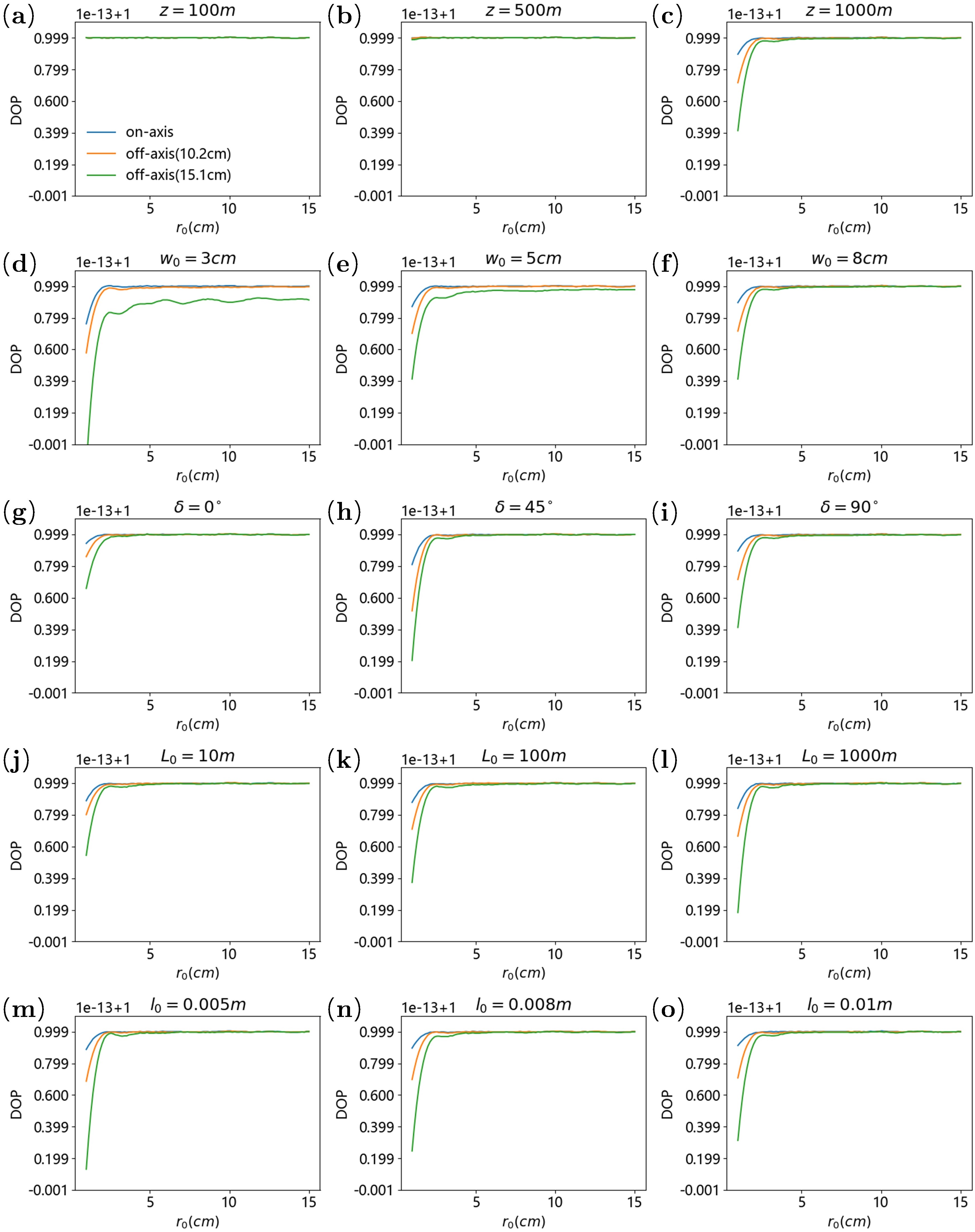
Figure 3: DOP of vector beams as a function of $r_{0}$ for different beam parameters and turbulence parameters, where each row from upper to bottom represents the results calculated under different propagation distances ((a) $z=100m$; (b) $z=500m$; (c) $z=1000m$), beam waists ((d) $w_{0}=3cm$; (e) $w_{0}=5cm$; (f) $w_{0}=8cm$), polarization types ((g) $\delta=0^{\circ}$; (h) $\delta=45^{\circ}$; (i) $\delta=90^{\circ}$), outer scales ((j) $L_{0}=10m$; (k) $L_{0}=100m$; (l) $L_{0}=1000m$) and inner scales ((m) $l_{0}=5mm$; (n) $l_{0}=8mm$; (o) $l_{0}=10mm$), respectively. All curves in each plot correspond to the DOP calculated under different off-axis magnitudes.

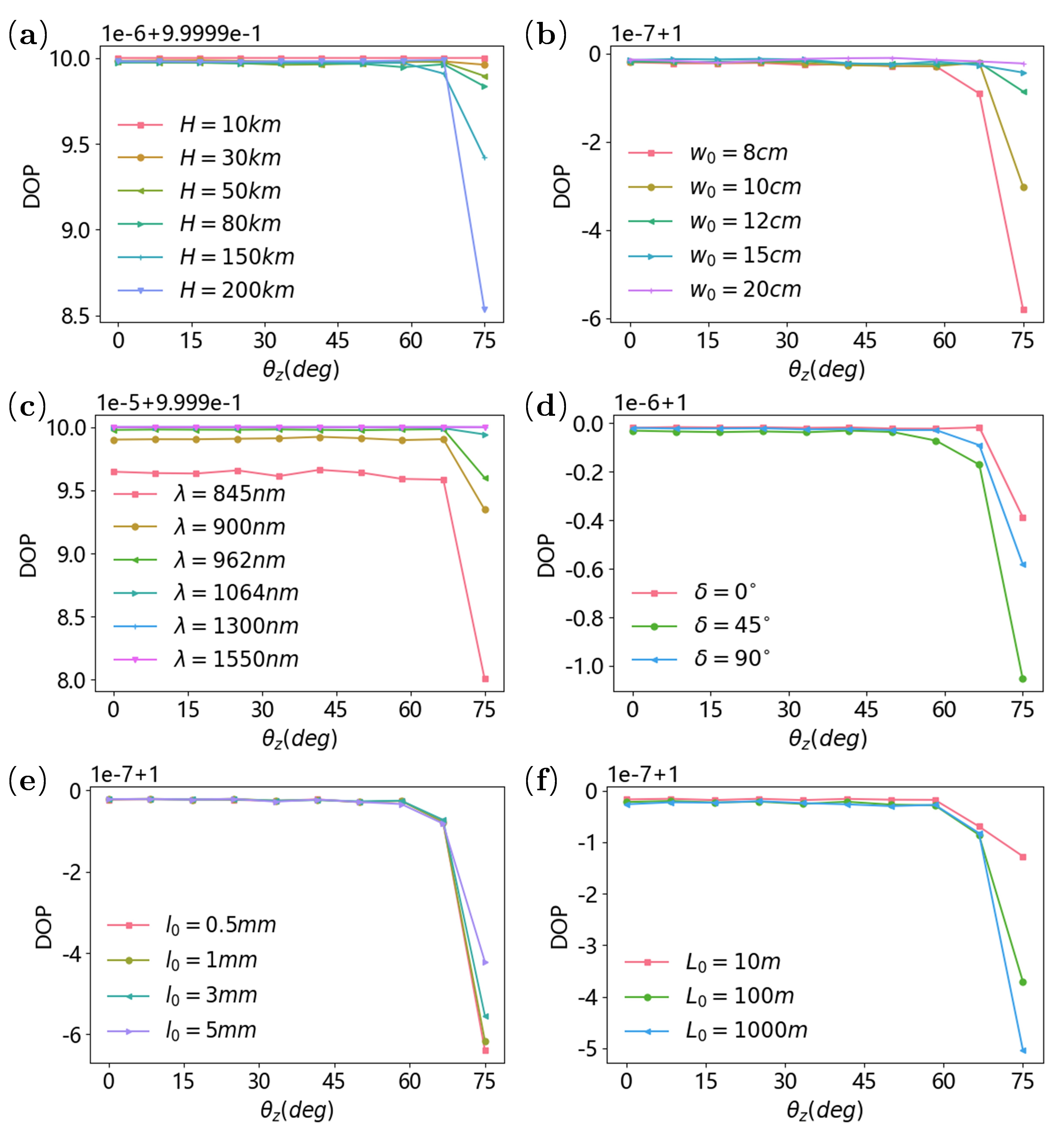
Figure 4: DOP of vector beams as a function of $\theta_{Z}$ for different beam parameters and turbulence parameters: (a) propagation distance; (b) beam waist; (c) wavelength; (d) polarization types; (e) inner scale; (f) outer scale. All curves in each plot correspond to the DOP calculated under different parameter settings.

The DOP of vector beams as a function of $r_{0}$ under different parameter settings, including beam parameters and turbulence parameters, are shown in Fig. 3, where each row from upper to bottom represents the results with different propagation distances $z$ (Fig. 3(a) to (c)), beam waists $w_{0}$ (Fig. 3(d) to (f)), polarization types $\delta$ (Fig. 3(g) to (i)), outer scales $L_{0}$ (Fig. 3(j) to (l)) and inner scale $l_{0}$ (Fig. 3(m) to (o)), respectively, where $\delta$ stands for the phase difference between $E_{x}^{\left(i\right)}$ and $E_{y}^{\left(i\right)}$. All curves in each plot correspond to the DOP under different off-axis magnitudes. As depicted in Fig. 3(a) to 3(c), we observe that DOP starts to decrease with the increasing propagation distance and turbulence strength, which is likely because the negative effects of turbulence on vector beams will become serious as the propagation distance increases. We also notice that in the short propagation distance or weak turbulence regime, the polarization properties remain almost constant and is hardly affected by the off-axis magnitude. Other than that, from the results presented in Fig. 3(d) to (f), we found that a smaller beam waist of vector beams may be lead to a strong effect of atmospheric turbulence. The primary reason because vector beams with a smaller beam waist possesses a larger divergence angle so that it is more susceptible to atmospheric turbulence[45]. The other conclusions about the effects of turbulence strength and off-axis magnitude are the same as those of Fig. 2. The effects of different polarization types at the transmitter on DOP with respect to $r_{0}$ are illustrated in Fig. 3(g) to (i). We notice that in the moderate-to-strong turbulence regime, the DOP of circularly polarized light may be more vulnerable to atmospheric turbulence than that of linearly polarized light; besides, when $\delta=45^{\circ}$, elliptically polarized light has the worst performance when propagating in atmospheric turbulence. Finally, we reveal the effects of outer scale and inner scale of turbulence on the DOP of vector beams in Fig. 3(j) to 3(o). From the comparison between different outer scales and inner scales, we observe that a large value of $L_{0}$ and a small value of $l_{0}$ may lead to a significant reduction of DOP, which is partly because inner scale and outer scale of turbulence forms the lower limit and upper limit of the inertial range, a smaller value of $l_{0}$ and a larger value of $L_{0}$ are obtained with the increase of turbulence strength. In the other words, the decreasing of $l_{0}$ or increasing of $L_{0}$ is equivalent to increase the number of turbulent cells along the turbulent channel, which causes a vector beam meets more turbulence during the atmospheric propagation.

3.2 Satellite-mediated links

After introducing the DOP of vector beams changes under different parameter settings in the free-space links, we now turn our attention to the satellited-mediated links. We further investigate whether the DOP of vector beams changes in the vertical atmospheric links, which can seen as a poster child of atmospheric propagation in long-distance and nonuniform turbulent links. The turbulence strength within a satellite-mediated atmospheric channel can be described by the refractive index structure parameter $C_{n}^{2}$ as a function of altitude $h$ (unlike the calculation of satellite-mediated atmospheric propagation, we keep $C_{n}^{2}$ constant in free-space links). We describe $C_{n}^{2}\left(h\right)$ by the widely used Hufnagel-Valley (HV) model[46] and adjust the distribution of turbulent cells by following the so-called rule of equivalent Rytov-index interval phase screen. More details about this rule and the turbulent link modeling used to perform the satellite-mediated calculation is further discussed in the Appendix. Notably, we adjust the side length at source plane and receiver plane with a specific value according to the propagation distance and beam waist during the satellite-mediated simulations because of the divergence properties of the vector beams propagating through atmospheric turbulence (e.g., when the propagation distance increases from $10km$ to $200km$, we set the side length at receiver plane from $1m$ to $3m$).

In Fig. 4, we illustrate the variation curves of the on-axis DOP of vector beams propagating through satellite-mediated links as a function of zenith angle $\theta_{Z}$ under different parameters (averaged over $1500$ realizations of turbulence). These parameters are the same as in Fig. 3. All curves in each plot correspond to the on-axis DOP under different parameter settings. We see in Fig. 4 that, overall, the DOP of vector beams remains almost unchanged with respect to $\theta_{Z}$ except when $\theta_{Z}$ becomes larger, however, the change of DOP in satellite-mediated links affected by atmospheric turbulence mainly fluctuates around the order of $10^{-5}$ to $10^{-7}$, which is negligible, but is more affected compared to the results achieved from free-space atmospheric propagation. As depicted in Fig. 4(a), we compare the on-axis DOP under different propagation distances (expressed as $H$). We found that in the large $\theta_{Z}$ regime, the DOP of long-distance propagation shows a significant reduction compare to that of short-distance one, which indicates that the DOP of on-axis optical field is gradually affected by atmospheric turbulence as the increase of propagation distance. In Fig. 4(b), we move our concern to the circumstance of different beam waists. We clearly observe the same conclusion obtained in the free-space links where the DOP of vector beams possessing a larger beam waist outperforms that of vector beams with a smaller one and once again verify the the primary reason that a smaller beam waist has a larger divergence angle so that it is more vulnerable in atmospheric turbulence whatever in free-space or satellite-mediated links. In Fig. 4(c), we calculate the DOP of a circularly-polorized vector beam propagating through vertical atmosphere under different values of wavelength. We clearly observe that the polarization properties is deeply affected by atmospheric turbulence with the decreasing wavelength (we use the word "deeply" to describe because the effect of wavelength on DOP varies in several orders of magnitude). In addition, we notice that the DOP is more affected by the wavelength for a larger $\theta_{Z}$, which may be caused by the combined effect of propagation distance and wavelength. We investigate the effects of different polarization types at the transmitter on DOP with respect to $\theta_{Z}$ in Fig. 4(d). We can easily achieve the same conclusion obtained in Fig. 3(g) to (i), namely, the elliptically polorized vector beam is more fragile compared to linearly and circularly polarized light. In a word, it should be emphasized that vector beams with different polarization types remain almost unaffected by atmospheric turbulence even in the satellite-mediated links. Fig. 4(e) and (f) plot the DOP of vector beams propagating in non-Kolmogorov turbulence as a function of $\theta_{Z}$ for different values of $l_{0}$ and $L_{0}$, where the calculation is shown for a distance of $150km.$ It can be seen that the smaller $l_{0}$ or the larger $L_{0}$ will always lead to a vector beam meet more turbulence either in the free-space or satellite-mediated propagation regime, for the reason we have already explained an intuitive way in the previous section.

4 Conclusions

In this paper, we have studied propagation of vector optical beams inside atmospheric turbulence, taking into account the change of polarization properties both in free-space links and satellite-mediated links. Unlike previous researches formulated by the cross-spectral density matrix[23, 24, 25, 26, 27, 28, 29, 30, 31, 32, 33, 34, 35, 36, 37], we propose a novel propagation model for a generally polarized vector beam in analogy with the well-known split-step beam propagation method. The main idea behind our method is that we consider the process of reflection and refraction exerted by a phase screen, which is derived on the generalization of the continuity of electromagnetic field. Additionally, we employ the vectorial diffraction formula to describe the vacuum diffraction between two phase screens. After making such revisions to the conventional propagation model, we investigate the change of polarization on atmospheric propagation under different parameters and parameter settings. It is found that the changes of DOP in free-space links and satellite-mediated links are mainly surrounded by the order of $10^{-13}$ and $10^{-6}$ and can nearly be ignored. Our results further confirmed vector beams whose DOP does not change on atmospheric propagation and will be useful for free-space optical communications and quantum communications.

Appendix A Satellite-mediated turbulent link modeling

We divide the satellite-mediated link into $N$ turbulent cells bounded by specific altitudes $h_{i}$ with $i$ ranging from $1$ to $N$ (note that turbulent cells are aranged from lower altitudes to higher altitudes). The altitude $h_{i}$ of each turbulent cell is calculated by the rule of equivalent Rytov-index interval phase screen (ERPS). For convenience of presentation, we summarize and divide the procedure of ERPS’s execution into four steps as follows (we employ the Rytov index $\sigma_{R}^{2}\left(\Delta h_{i}\right)$ to characterize the scintillation between two turbulent cells, see more detailed reasons in Ref. [47]):

1) We set the constant $c$ such that the Rytov index of two adjacent phase screens is equal to $c$ (i.e., $\sigma_{R}^{2}\left(\Delta h_{i}\right)\equiv c$, where $\Delta h_{i}=h_{i+1}-h_{i}$).

2) We calculate the altitude of the first phase screen based on $C_{n}^{2}\left(0\right)$ (represent the near-surface refractive index structure parameter) and the Rytov equation: $\sigma_{R}^{2}\left(\Delta h_{1}\right)=1.23C_{n}^{2}\left(0\right)k^{7/6}\left(\Delta h_{1}\right)^{11/6}\equiv c$, which is employed to set the initial value.

3) We calculate the spacing $\Delta h_{i}$ by using $C_{n}^{2}\left(h_{i}\right)$ and solving the identity: $1.23C_{n}^{2}\left(h_{i}\right)k^{7/6}\left(\Delta h_{i}\right)^{11/6}\equiv c$.

4) We repeat step 3) several times until the sum of the spacing of phase screen equals the total propagation distance (i.e., we should decide whether $\sum_{i=1}^{N}\Delta h_{i}$ is equal to $H$. If not, we repeat step 3; if yes, we terminate the loop).

So far, we have determined the exact number of $N$ and obtained the specific altitudes of $h_{i}$. However, it is worth emphasizing that the above calculation is performed assuming the condition that $\theta_{Z}=0$. If $\theta_{Z}\neq 0$, the specific altitudes of turbulent cells should be adjusted to $h_{1}\sec\theta_{Z}$, $h_{2}\sec\theta_{Z}$, $\cdots$, $h_{N}\sec\theta_{Z}$.

Finally, we realize the corresponding random phase screens by employing the von-Karman spectrum of refractive-index fluctuation[48] and the well-known subharmonic-conpensation-based fast-Fourier-transform algorithm[41, 42, 49, 50], which is implemented on the python library named AOtools[51].

Funding. HFIPS Director’s Foundation (YZJJ2023QN05); National Key R$\&$D Program of China (2019YFA0706004); National Natural Science Foundation of China (11904369); National Key R$\&$D Program of Young Scientists (SQ2022YFF1300182); Youth Innovation Promotion Association of Chinese Academy of Sciences (2022450).

Acknowledgment. We would like to thank the anonymous reviewers for their valuable comments, which significantly improves the presentation of this paper.

Disclosures. The authors declare no conflicts of interest.

^†These authors contributed equally to this article.

References

- [1] A. Z. Goldberg, P. de la Hoz, G. Bjork, A. B. Klimov, M. Grassl, G. Leuchs, and L. L. Sanchez-Soto, "Quantum concepts in optical polarization," Adv. Opt. Photon. 13, 1–73 (2021).
- [2] A. Muller, J. Breguet, and N. Gisin, "Experimental demonstration of quantum cryptography using polarized photons in optical fibre over more than 1 km," Europhys. Lett. 23, 383 (1993).
- [3] K. Mattle, H. Weinfurter, P. G. Kwiat, and A. Zeilinger, "Dense coding in experimental quantum communication," Phys. Rev. Lett. 76, 4656–4659 (1996).
- [4] D. Bouwmeester, J.-W. Pan, K. Mattle, M. Eibl, H. Weinfurter, and A. Zeilinger, "Experimental quantum teleportation," Nature 390, 575–579 (1997).
- [5] M. Rådmark, M. Żukowski, and M. Bourennane, "Experimental high fidelity six-photon entangled state for telecloning protocols," New J. Phys. 11, 103016 (2009).
- [6] K. J. Resch, K. L. Pregnell, R. Prevedel, A. Gilchrist, G. J. Pryde, J. L. O’Brien, and A. G. White, "Time-reversal and super-resolving phase measurements," Phys. Rev. Lett. 98, 223601 (2007).
- [7] P. B. Dixon, D. J. Starling, A. N. Jordan, and J. C. Howell, "Ultrasensitive beam deflection measurement via interferometric weak value amplification," Phys. Rev. Lett. 102, 173601 (2009).
- [8] G. G. Stokes, "On the composition and resolution of streams of polarized light from different sources," Trans. Cambridge Phil. Soc. 9, 399–416 (1852).
- [9] E. Wolf, "Optics in terms of observable quantities," Nuovo Cimento 12, 884–888 (1954).
- [10] W. H. McMaster, "Polarization and the Stokes parameters," Am. J. Phys. 22, 351–362 (1954).
- [11] M. J. Walker, "Matrix calculus and the Stokes parameters of polarized radiation," Am. J. Phys. 22, 170–174 (1954).
- [12] R. Barakat, “Statistics of the Stokes parameters,” J. Opt. Soc. Am. A 4, 1256–1263 (1987).
- [13] H. Poincaré, Théorie Mathématique de la Lumière (Georges Carré, 1889).
- [14] E. Wolf, Introduction to the Theory of Coherence and Polarization of Light (Cambridge University, 2007).
- [15] P. Réfrégier and A. Roueff, "Intrinsic coherence: a new concept in polarization and coherence theory," Opt. Photon. News 18, 30–35 (2007).
- [16] E. Wolf, "Unified theory of coherence and polarization of random electromagnetic beams," Phys. Lett. A. 312, 263–267 (2003).
- [17] J. H. Eberly, X.-F. Qian, and A. N. Vamivakas, "Polarization coherence theorem," Optica 4, 1113–1114 (2017).
- [18] H. Roychowdhury and E. Wolf, "Determination of the electric cross-spectral density matrix of a random electromagnetic beam," Opt. Commun. 266, 57 (2003).
- [19] S. Joshi, S. N. Khan, Manisha, P. Senthilkumaran, and B. Kanseri, "Coherence-induced polarization effects in vector vortex beams," Opt. Lett. 45, 4815–4818 (2020).
- [20] M. Salem and E. Wolf, "Coherence-induced polarization changes in light beams," Opt. Lett. 33, 1180–1182 (2008).
- [21] O. Korotkova, B. G. Hoover, V. L. Gamiz, and E. Wolf, "Coherence and polarization properties of far fields generated by quasi-homogeneous planar electromagnetic sources," J. Opt. Soc. Am. A 22, 2547–2556 (2005).
- [22] S. Joshi, S. N. Khan, P. Senthilkumaran, and B. Kanseri, "Statistical properties of partially coherent polarization singular vector beams," Phys. Rev. A 103, 053502 (2021).
- [23] E. Wolf, "Correlation-induced changes in the degree of polarization, the degree of coherence, and the spectrum of random electromagnetic beams on propagation," Opt. Lett. 28, 1078–1080 (2003).
- [24] O. Korotkova and E. Wolf, "Changes in the state of polarization of a random electromagnetic beam on propagation," Opt. Commun. 246, 35–43 (2005).
- [25] E. Wolf, "Polarization invariance in beam propagation," Opt. Lett. 32, 3400–3401 (2007).
- [26] D. Zhao and E. Wolf, "Light beams whose degree of polarization does not change on propagation," Opt. Commun. 281, 3067–3070 (2008).
- [27] R. Martinez-Herrero and P. M. Mejias, "Electromagnetic fields that remain totally polarized under propagation," Opt. Commun. 279, 20–22 (2007).
- [28] X. Zhao, Y. Yao, Y. Sun, and C. Liu, "Condition for Gaussian Schell-model beam to maintain the state of polarization on the propagation in free space," Opt. Express 17, 17888–17894 (2009).
- [29] G. P. Agrawal and E. Wolf, "Propagation-induced polarization changes in partially coherent optical beams," J. Opt. Soc. Am. A 17, 2019–2023 (2000).
- [30] X. Du and D. Zhao, "Criterion for keeping completely unpolarized or completely polarized stochastic electromagnetic Gaussian Schell-model beams on propagation," Opt. Express 16, 16172–16180 (2008).
- [31] E. Wolf, “Invariance of spectrum of light on propagation,” Phys. Rev. Lett. 56, 1370–1372 (1986).
- [32] D. F. V. James, "Change of polarization of light beams on propagation in free space," J. Opt. Soc. Am. A 11, 1641–1643 (1994).
- [33] J. Wu, J. Ma, L. Tan, and S. Yu, "Condition for keeping polarization invariant on propagation in space-to-ground optical communication downlink," Opt. Commun. 453, 124410 (2019).
- [34] H. Roychowdhury, S. A. Ponomarenko, and E. Wolf, "Change of polarization of partially coherent electromagnetic beams propagating through the turbulent atmosphere," J. Mod. Opt. 52, 1611–1618 (2005).
- [35] J. Wu, J. Ma, L. Tan, and S. Yu, "Polarization invariance in beam propagation for space-to ground optical communication downlink," in Conference on Lasers and Electro-Optics, OSA Technical Digest (online) (Optica Publishing Group, 2017), paper JTh2A.4.
- [36] J. Zhang, S. Ding, H. Zhai, and A. Dang, "Theoretical and experimental studies of polarization fluctuations over atmospheric turbulent channels for wireless optical communication systems," Opt. Express 22, 32482–32488 (2014).
- [37] T. Shirai and E. Wolf, "Coherence and polarization of electromagnetic beams modulated by random phase screens and their changes on propagation in free space," J. Opt. Soc. Am. A 21, 1907–1916 (2004).
- [38] M. Born and E. Wolf, Principles of Optics, sixth ed. (Pergamon Press, Oxford, England, 1993).
- [39] E. Hechit, Optics, 3rd ed. (Addison-Wesley, Reading, Mass., 1998).
- [40] https://en.wikipedia.org/wiki/Fresnel_equations.
- [41] J. D. Schmidt, Numerical Simulation of Optical Wave Propagation with Examples in MATLAB (SPIE, 2010).
- [42] G. Sedmak, "Implementation of fast-Fourier-transform-based simulations of extra-large atmospheric phase and scintillation screens," Appl. Opt. 43, 4527–4538 (2004).
- [43] J. W. Goodman, "Introduction to Fourier optics. 3rd," Roberts and Company Publishers3 (2005).
- [44] J. A. Stratton and L. J. Chu, "Diffraction Theory of Electromagnetic Waves," Phys. Rev. 56, 99–107 (1939).
- [45] M. J. Padgett, F. M. Miatto, M. P. J. Lavery, A. Zeilinger, and R. W. Boyd, "Divergence of an orbital-angular-momentum-carrying beam upon propagation," New J. Phys. 17, 023011 (2015).
- [46] R. Hufnagel and N. R. Stanley, "Modulation transfer function associated with image transmission through turbulent media," J. Opt. Soc. Am. 54, 52 (1964).
- [47] Z. Tao, Y. Ren, A. Abdukirim, S. Liu, and R. Rao, "Physical meaning of the deviation scale under arbitrary turbulence strengths of optical orbital angular momentum," J. Opt. Soc. Am. A 38, 1120-1129 (2021).
- [48] L. C. Andrews and R. L. Phillips, Laser Beam Propagation through Random Media, 2nd ed. (SPIE, 2005).
- [49] J. M. Martin and Stanley M. Flatte, "Intensity images and statistics from numerical simulation of wave propagation in 3-D random media," Appl. Opt. 27, 2111-2126 (1988).
- [50] B. M. Welsh, “Fourier-series-based atmospheric phase screen generator for simulating nonisoplanatic geometries and temporal evolution,” Proc. SPIE 3125, 327–338 (1997).
- [51] M. J. Townson, O. J. D. Farley, G. Orban de Xivry, J. Osborn, and A. P. Reeves, "AOtools: a Python package for adaptive optics modelling and analysis," Opt. Express 27, 31316-31329 (2019).