Q-ball-like solitons on the M2-brane with worldvolume fluxes

Abstract

In this paper we obtain a family of analytic solutions to the nonlinear partial differential equations that describe the dynamics of the bosonic part of a M2-brane compactified on $M_{9}\times T^{2}$ in the LCG with worldvolume fluxes. Those fluxes can be induced by a constant and quantized supergravity 3-form. This sector of the theory, at supersymmetric level, has the interesting property of having a discrete spectrum. In this paper we focus in the characterization of Q-ball solitons on the M2-brane with worldvolume fluxes. We obtain two analytic families of Q-ball-like solutions that satisfy all of the constraints. We analyze two different scenarios: one in which the system is in an isotropic case and other one, anisotropic. In the first case, we obtain two analytic families of solutions in the presence of a non-vanishing symplectic gauge field. We show that the solutions exhibit generically dispersion although they also admit solutions dispersion-free. We obtain the superposition law of the analytic solutions. They admit linear superposition but only for restricted discrete frequencies. In the non-isotropic case, we show numerically, that the system also admits Q-ball solutions, even for the simple backgrounds like the one that we are considering. The dynamics of the Q-balls are also encountered. We analyze the Lorentz boosts and Galilean transformations. Since we work in the light cone gauge, the Lorentz transformed solutions are not automatically solutions, rather some conditions must be imposed. Only a subset of the solutions remain. We discuss some examples. The Q-ball solitons of the M2-brane have a mass term that contains an interaction term between the Noether charge of the Q-ball and the topological monopole charge associated with the worldvolume flux. These solutions could be related to a new type of solitons denoted as Q-monopole-ball, although in order to determine it a more profound study is required.

1 Introduction

Solitons are stable classical solutions with finite energy to nonlinear equations that are able to mimick the behaviour of particles as well as excitations. They are classified into topological and nontopological ones. Topological solitons like monopoles, vortices, instantons and kinks have been extensively studied in the literature. Non-topological solitons have also received a lot of interest for its potential to explain dark matter among others. One simple case corresponds to Q-balls. Q-balls COLEMAN1985263 are the generic name given to solitons, originally with spherical topology, which are invariant under a $U(1)$ global symmetry. This symmetry implies the existence of a Noether charge which provides stability against perturbations. Thus global symmetry has been associated to quantum invariants as lepton or barion number. There exists also gauged Q-balls Q-ballUgauged ; MappinggaugedQ-balls in the case in which the complex scalar fields that parametrized the Q-ball are also charged under a gauge potential $U(1)$. There are also other works in which the authors have considered more general global or gauged groups Loginov2007 ; ALONSOIZQUIERDO2023 . Dynamics of Q-balls have been studied in Floratos:2000-Qballs ; DynamicsQ-ballsExpandingUniverse and for the gauged case Q-ballUgauged ; Gulamov_2015 . Their stability has also been discussed in several papers, see for example ThePhysicsofQballsThesis . Recently, it has been discovered that it is possible to obtain solitonic solutions that simultaneously share the two types of properties. These type of solitons have been denoted as Q-monopole-ball Bai2022 .

Solitons with other topologies different from the sphere have been described to less extent ALONSOIZQUIERDO2022 . For example, Q-torus, which corresponds to Q-balls with toroidal topology have been also studied in Q-TorusInN2SupersimetricQED . Q-balls have also been used to model dark matter art:Supersymmetric_Qballs_as_dark_matterKusenko:1997si or like FQuevedo:ModuliStarKrippendorf2018 in the context of String theory. This last one describes Q-ball solitons from the open and closed string moduli as well as other type of solitons. However, there are very few results of solitons reported at the level of M-theory.

Classical solutions of membrane theory can be useful to understand better the M-theory properties of its fundamental elements. First examples of classical solutions to the membrane theory firstly appeared in nicolaihoppe . In the context of matrix models, it was discussed in Hoppe:1997SolutionsMatrixModelEquations . The existence of membrane solitonic solutions has been discussed in several works. For example in terms of stringy solitary waves in Restuccia:1998_MembraneSolitons , in the context of Q-ball matrix model Soo-Jong_Rey , as instantonic solutions FLORATOS:1998_InstantonSolutionsSelf-dualMembrane , or in terms of membranes formulated on hyperkähler backgrounds Bergshoeff:1999_SolitonsOnSupermembrane ; Portugues_2004 . There are bounds for the experimental detection of Q-balls ThePhysicsofQballsThesis , though they are model dependent.

In this paper we obtain the first exact Q-ball-like soliton solutions for the M2-brane with worldvolume fluxes. We consider a supermembrane on a $M_{9}\times T^{2}$ target space with a $C_{\pm}$ flux background. This configuration possesses a magnetic $U(1)$ monopole in the compact sector mpdm2019:flux ; mpgm10Monodromy associated to the flux content that induces the presence of a magnetic monopole over the worldvolume MARTINRestucciaTorrealba1998:StabilityM2Compactified . We search solutions to the nonlinear equations of the M2-brane on this particular background focusing on the existence of Q-ball-like solitons. The Hamiltonian that describes the dynamics of the M2-brane contains not only nontrivial topological terms but also a symplectic field strength. We obtain Q-ball-like analytical solutions to the problem in the isotropic case, by solving the equations of motion (EOM) and the constraints of the theory: the area preserving first class constraint and the flux constraint. This last one induces a topological central charge restriction. We show that for the enalytic families of solutions considered, they exhibit generically dispersion although they also admit solutions dispersion-free. We characterize their superposition law. With the aid of numerical simulation, we extend those results to the non-isotropic case in the absence of a symplectic gauge field. We obtain Q-ball-like soliton solutions described by the complex scalars that parametrize the position of the M2-brane in the noncompact transverse space to the light cone coordinates. We also obtain the dynamics of the Q-ball by studying the Lorentz transformation and its nonrelativistic limit the Galilean one. Since we are in the Light Cone Gauge (LCG) the transformed solutions are not automatically solutions and it must be checked for each class of solutions. The M2-brane in those cases contains a monopole associated to the nontrivial embedding in the compact space as well as Q-ball solitons associated with the noncompact directions. Both terms, furthermore, interact non-trivially at the level of the mass operator through the covariant derivative terms, leading to greater stability of the Q-ball solitons. They can constitute a new example of the recently identified Q-monopole-ball soliton.

The paper is structured as follows: In section 2 we review the formulation of the supermembrane toroidally wrapped on $M_{9}\times T^{2}$ subject to a $C_{\pm}$ flux condition and the equations of motion to solve them. From section 3 to section 8. we present our results. In section 3. we obtain analytically a family of exact Q-ball-like (QBL) solutions for an isotropic case. We characterize the dispersion of the solutions in the presence of a symplectic gauge field. In section 4. we obtain a superposition law for the QBL family of solutions previously found. We find that for the isotropic case it is possible to linearly overlap the solutions but only when the frequencies become strongly restricted. This is consistent with the nonlinear character of the equations. In section 5. we characterize a Q-ball numerically comparing with the analytical results in the isotropic case and extending them to the non-isotropic case, when the symplectic gauge vanishes. In the non-isotropic case, the nonlinear character of the complex scalar field becomes explicitly manifest. In section 6 we discuss the dynamics of the solutions by considering a Lorentz boost and its nonrelativistic limit a galilean transformation. In section 7, we show that there exists a relation between the topological and non-topological charges of the M2-brane. In section 8 we discuss the results obtained and conclude.

2 The M2-brane with 2-form worldvolume $C_{\pm}$ fluxes

In this work we analyze the existence of solutions to the dynamics of an M2-brane mass operator, focusing in those of Q-ball-type. The bosonic sector that we analyze, corresponds to the supermembrane with $C$ fluxes introduced in mpdm2019:flux ; mpgm10Monodromy that induce a topological condition denoted central charges which is associated with the presence of a magnetic monopole over the worldvolume of the membrane MARTINRestucciaTorrealba1998:StabilityM2Compactified . The M2-brane is formulated on a target space $M_{9}\times T^{2}$ in the Light Cone Gauge (LCG) Ovalle1 ; Ovalle2 . We define the embedding maps on the non-compact space $X^{m}(\tau,\sigma,\rho):\Sigma\to M_{9}$ with $m=2,...,8$. The maps $X^{r}(\tau,\sigma,\rho):\Sigma\to T^{2}$, where $r=9,10$, describe the embedding on the compactified 2-torus. These maps act as scalars on the M2-brane worldvolume and as vectors on the target space. The supermembrane worldvolume coordinates are labeled by $(\tau,\sigma,\rho)$ parametrizing $\Sigma\times\mathbb{R}$, with $\Sigma$ representing a Riemann surface of genus one and $\mathbb{R}$ parametrizing time. The maps $X^{r}$ satisfy the winding condition

$$\oint_{\mathcal{C}_{s}}dX^{r}=2\pi R^{r}m_{r}^{s}\ ,$$ (1)

where $m_{r}^{s}$ are the winding numbers and $R^{r}$ are the torus radii. The M2-brane is restricted by a worldvolume flux condition

$$\int_{T^{2}}F_{2}=n\in\mathbb{Z}/\{0\}.$$ (2)

The worldvolume flux can be also induced by the pullback of a target-space flux condition, see, for example, in mpdm2019:flux ; mpgm10Monodromy . In both cases it is defined in terms of an integer $n$. It also corresponds to a topological condition denoted by the authors as Central Charge condition(CC) MARTINRestucciaTorrealba1998:StabilityM2Compactified , satisfying that $n=det\mathbb{W}$ where $\mathbb{W}$ denotes the winding matrix of an irreducible wrapping of the M2-brane around the compactified 2-torus. The central charge condition is associated to the existence of a monopole over the worldvolume which is given by the curvature $\widehat{F}=\epsilon_{rs}dX^{r}_{h}\wedge dX^{s}_{h}$ associated to a nontrivial $U(1)$ gauge field $\widehat{F}=d\widehat{A}$ defined on the membrane worldvolume.

$$\int_{\Sigma}\widehat{F}=\int_{\Sigma}dX^{r}\wedge dX^{s}=\epsilon^{rs}nA_{T^{2}},\quad n\in\mathbb{Z}/\{0\}\ ,$$ (3)

where $A_{T^{2}}$ denotes the 2-torus target space area. The associated closed one-forms $dX_{r}$ can be decomposed by a Hodge decomposition in terms of two harmonic one-forms $d\widehat{X}_{r}$ and two exact one-forms $dA_{r}$, such that

$$dX_{r}(\sigma,\rho,\tau)=d{X}_{rh}(\sigma,\rho)+dA_{r}(\sigma,\rho,\tau)\,,$$ (4)

The $dX_{rh}$ is a closed one-form defined in terms of the basis of harmonic forms as $d{X}_{rh}=R^{r}m_{r}^{s}d\widehat{X}_{s}(\sigma,\rho)$. The central charge condition guarantees the existence of the two independent harmonic constant one-forms, $d\widehat{X}_{s}(\sigma,\rho)$. The central charge condition also implies the existence a new dynamical degree of freedom $A_{r}$ whose associated one-form $\mathbb{A}_{r}=dA_{r}=\partial_{a}A_{r}d\sigma^{a}$, with $\partial_{a}=(\partial_{\sigma},\partial_{\rho})$ describes a symplectic gauge field over the M2-brane worldvolume. It transforms as a symplectic connection under symplectomorphisms. $dA_{r}$ are exact one-forms.

The LCG Hamiltonian of the M2-brane theory with central charge corresponds to Ovalle1 ; Ovalle2

$$H_{CC} =T^{-2/3}\int_{\Sigma}d^{2}\sigma\sqrt{W}\Big{[}\frac{1}{2}\Big{(}\frac{P_{m}}{\sqrt{W}}\Big{)}^{2}+\frac{1}{2}\Big{(}\frac{P_{r}}{\sqrt{W}}\Big{)}^{2}\Big{]}$$ (5)

$$+T^{-2/3}\int_{\Sigma}d^{2}\sigma\sqrt{W}\Big{[}\frac{T^{2}}{4}\left\{X^{m},X^{n}\right\}^{2}+\frac{T^{2}}{2}(\mathcal{D}_{r}X^{m})^{2}+\frac{T^{2}}{4}(\mathcal{F}_{rs})^{2}\Big{]},$$

where $T$ stands for the membrane tension and $W$ is the determinant of the induced spatial part component of the foliated metric on the membrane; $\left\{A,B\right\}=\frac{1}{\sqrt{W}}\epsilon^{ab}\partial_{a}A\partial_{b}B;\$ is the symplectic bracket defined in terms of the harmonic one-forms $d\widehat{X}$ of the Riemann surface with $a,b=1,2$ and $\partial_{a}=(\partial_{\sigma},\partial_{\rho})$ and $\sqrt{W}=\frac{1}{2}\epsilon^{ab}\epsilon_{rs}\partial_{a}\widehat{X}^{r}\partial_{b}\widehat{X}^{s}$. The scalar fields $X^{m},A_{r}$ have respectively, canonical momenta $P_{m}$ and $P_{r}$. The symplectic covariant derivative is defined as $\mathcal{D}_{r}\bullet=D_{r}\bullet+\{A_{r},\bullet\}$ with $D_{r}\bullet=2\pi m_{r}^{u}\theta_{uv}R_{r}\frac{\epsilon^{{a}{b}}}{\sqrt{W}}\partial_{{a}}\widehat{X}^{v}\partial_{{b}}\bullet.$   The derivative $D_{r}$ is defined in terms of the moduli of the 2-torus, the harmonic one-forms $d\widehat{X}_{r}$, and a matrix $\theta_{uv}$ with $u,v=9,10$, related to the monodromy associated to its global description in terms of a torus bundle GMPR2012 . Therefore, the Hamiltonian contains a symplectic curvature $\mathcal{F}$ defined by

$$\mathcal{F}_{rs}=D_{r}A_{s}-D_{s}A_{r}+\left\{A_{r},A_{s}\right\}.\,$$ (6)

The constraints of the theory associated to the local Area Preserving Diffeomorphisms (APD) are:

$$\mathcal{D}_{r}P_{r}+\left\{X^{m},P_{m}\right\}\approx 0\ ,$$ (7)

and to the two APD global constraints,

$$\oint_{\mathcal{C}_{s}}\Big{(}\Big{(}\frac{P_{r}}{\sqrt{W}}\Big{)}\partial_{a}X^{r}+\Big{(}\frac{P_{m}}{\sqrt{W}}\Big{)}\partial_{a}X^{m}\Big{)}d\sigma^{a}\approx 0\ .$$ (8)

In the dynamics of the M2-brane we will only be concerned with the local area preserving diffeomorphisms constraint and the flux constraint.

The fluxes of the Hamiltonian can be induced by the presence of a constant quantized 3-form $C_{\pm}$ background. The Hamiltonian of a supermembrane with central charges corresponds to the Hamiltonian of the M2-brane with worldvolume fluxes $C_{-}$. Its formulation is equivalent to the Hamiltonian of the M2-brane with central charge, plus a constant shift given by the pullback of the $C_{+}$ contribution mpdm2019:flux ; mpgm10Monodromy

$$H_{C_{\pm}}^{fluxes}=H_{C_{-}}+\int_{\Sigma}C_{+}=H_{CC}+\int_{\Sigma}C_{+}\ .$$ (9)

The dynamics of the M2-brane with worldvolume fluxes is determined by the equations of motion (EOM) and their constraints. The Lagrangian density of the theory can be obtained by performing a usual Legendre transformation of the Hamiltonian density defined as

$$\mathcal{H}_{T}=\sqrt{W}\mathcal{H}_{c}+\Lambda\phi,$$ (10)

where $\Lambda$ represents a Lagrange multiplier and $\phi=-\phi_{APD}$ represents the APD constraint given by equation (7). It contains the Lagrangian of MIM2, formerly obtained in Bellorin:Restuccia:2003 , plus a constant term associated to the flux contribution $K$.

$$S=\int d\tau d\sigma^{2}\mathcal{L}_{T}=-\int d\tau d\sigma^{2}\sqrt{W}\Big{[}\frac{1}{2}(D_{i}{X}_{m})^{2}+\frac{1}{4}\left\{X_{m},X_{n}\right\}^{2}+\frac{1}{4}\mathcal{F}_{ij}^{2}\Big{]}+K.$$ (11)

The tension has been fixed to $T=1$. Since the $K$ contribution gives a constant term, added to the action. Its equations of motion are equal to those of the M2-brane with central charges. The symplectic field strength, and the symplectic covariant derivative now run over the indices $i,j=0$, $r=9,10$ with $A_{0}=\Lambda$ and $D_{0}=\partial_{\tau}$. As explained in Hoppe:PhdTesis ; Allen:Andersson:Restuccia:2010 the gauge freedom of the system allows to fix $\Lambda=0$ and then the Lagrangian density function $\mathcal{L}=\mathcal{L}_{T}-K$ reduces to

$$\sqrt{W}^{-1}\mathcal{L}=\frac{1}{2}[(\dot{X}_{m})^{2}+(\dot{A}_{r})^{2}]-\frac{1}{4}\left\{X_{m},X_{n}\right\}^{2}-\frac{1}{2}\left(\mathcal{D}_{r}X_{m}\right)^{2}-\frac{1}{4}\mathcal{F}_{rs}^{2}$$ (12)

The nonlinear system of equations that one has to solve is the following: From (12) we derive the equations of motion for the dynamical fields $X^{m}(\tau,\sigma,\rho)$ and $A_{r}(\tau,\sigma,\rho)$

$$\ddot{X}^{m}(\tau,\sigma,\rho)=\left\{X_{n},\left\{X^{n},X^{m}\right\}\right\}+\left\{{X}_{r},\mathcal{D}^{r}{X}^{m}\right\}\ ,$$ (13)

$$\ddot{A}_{r}(\tau,\sigma,\rho)=\left\{\mathcal{D}_{r}X^{m},X_{m}\right\}+\left\{\mathcal{F}_{rs},{X}^{s}\right\}\ ,$$ (14)

subject to satisfy the APD constraint of the theory

$$\mathcal{D}_{r}\Big{(}\dot{A}_{r}\Big{)}+\left\{X^{m},\dot{X}^{m}\right\}=0\,\quad\text{for}\quad r=9,10,$$ (15)

and the worldvolume flux condition (3), that restricts the winding numbers allowed for the M2-brane.

In order to find the admissible M2-brane solutions, the system of equations (13), (14), (15) and (3) must be solved. For simplicity we will also assume that one of the scalar fields constant and we will fix the harmonic sector as in BRR2005nonperturbative ,

$$X_{2}=constant,\quad X_{h_{r}}=R_{r}(n_{r}\sigma+m_{r}\rho),\quad r=9,10.$$ (16)

For this ansatz $\sqrt{W}=1$. There are some differences with the case analyzed in BRR2005nonperturbative . The main one is associated with the fact that for the supersymetric M2-brane, the worldvolume flux condition guarantees the discreteness of the spectrum. Other difference due to the topological restriction imposed is that appearance of new single-valued degrees of freedom, $A_{r}$ that are components of a symplectic gauge connection $\mathbb{A}=dA_{r}$ in the theory. The EOM for $X_{2}$ constant, can be expressed in terms of complex variables $Z_{a}$ with $a=1,2,3$ where $Z_{a}(\tau,\sigma,\rho)=X_{2a+1}+iX_{2a+2}$. They are,

$$\ddot{Z}_{c} = \frac{1}{2}\sum_{a=1}^{3}\left(\left\{\left\{Z_{c},Z_{a}\right\},\overline{Z}_{a}\right\}+\left\{\left\{Z_{c},\overline{Z}_{a}\right\},{Z}_{a}\right\}\right)+\sum_{r=9}^{10}\left\{X_{r},\mathcal{D}_{r}Z_{c}\right\},$$ (17)

$$\ddot{A}_{r} = \frac{1}{2}\sum_{a=1}^{3}\left(\left\{\mathcal{D}_{r}Z_{a},\overline{Z}_{a}\right\}+\left\{\mathcal{D}_{r}\overline{Z}_{a},Z_{a}\right\}\right)+\sum_{s=9}^{10}\left\{\mathcal{F}_{rs},X^{s}\right\}\ ,$$ (18)

subject to the APD constraint of the theory:

$$\frac{1}{2}\sum_{c=1}^{3}\left(\left\{\dot{Z}_{c},\bar{Z}_{c}\right\}+\left\{\dot{\bar{Z}}_{c},Z_{c}\right\}\right)-\mathcal{D}_{r}\dot{A}_{r}=0\ .$$ (19)

In the following we assume the Q-ball ansatz for the complex scalars $Z_{a}$. We will denote this last ansatz as ’Q-ball like’ (QBL) irrespective of its toroidal topology associated to the membrane worldvolume

$$Z_{a}=f_{a}(\sigma,\rho)e^{i\omega_{a}\tau},\quad\text{with}\quad f(\sigma,\rho)\in\mathbb{R}\,.$$ (20)

The EOM for $Z_{a}$ become

$$\omega_{c}^{2}f_{c}= - \sum_{r=9}^{10}\left[\partial_{\sigma}^{2}f_{c}\left[R_{r}m_{r}+\partial_{\rho}A_{r}\right]^{2}+\partial_{\rho}^{2}f_{c}\left(R_{r}n_{r}+\partial_{\sigma}A_{r}\right)^{2}\right]$$

$$+ \sum_{r=9}^{10}\partial_{\sigma\rho}^{2}f_{c}\left[2\ \left(R_{r}n_{r}+\partial_{\sigma}A_{r}\right)\left(R_{r}m_{r}+\partial_{\rho}A_{r}\right)\right]$$

$$+ \sum_{r}\left[\partial_{\sigma}^{2}A^{r}\partial_{\rho}f_{c}\left(R_{r}m_{r}+\partial_{\rho}A_{r}\right)+\partial_{\rho}^{2}A^{r}\partial_{\sigma}f_{c}\left(R_{r}n_{r}+\partial_{\sigma}A_{r}\right)\right]$$

$$- \sum_{r}\partial_{\sigma\rho}^{2}A_{r}\left[\partial_{\sigma}f_{c}\left(R_{r}m_{r}+\partial_{\rho}A_{r}\right)+\partial_{\rho}f_{c}\left(R_{r}n_{r}+\partial_{\sigma}A_{r}\right)\right]$$

$$- \sum_{a}\left[\partial_{\sigma}^{2}f_{c}(\partial_{\rho}f_{a})^{2}-2\partial_{\sigma\rho}^{2}f_{c}\left[\partial_{\sigma}f_{a}\partial_{\rho}{f}_{a}\right]+\partial_{\rho}^{2}f_{c}\left(\partial_{\sigma}f_{a}\right)^{2}\right]$$

$$+ \sum_{a}\left[\partial_{\rho}^{2}f_{a}\partial_{\sigma}f_{c}\partial_{\sigma}{f}_{a}-\partial_{\sigma\rho}^{2}f_{a}(\partial_{\sigma}f_{c}\partial_{\rho}{f}_{a}+\partial_{\rho}f_{c}\partial_{\sigma}{f}_{a})+\partial_{\sigma}^{2}f_{a}\partial_{\rho}f_{c}\partial_{\rho}{f}_{a}\right]\ .$$

The EOM for $A_{r}$ are:

$$\ddot{A}_{r}= - \sum_{a=1}^{3}\left[\partial_{\sigma}^{2}f_{a}\ \partial_{\rho}{f}_{a}\left(R_{r}m_{r}+\partial_{\rho}A_{r}\right)+\partial_{\rho}^{2}f_{a}\ \partial_{\sigma}{f}_{a}\left(R_{r}n_{r}+\partial_{\sigma}A_{r}\right)\right]$$

$$+ \sum_{a=1}^{3}\left[\partial_{\sigma\rho}^{2}f_{a}\left[\partial_{\rho}{f}_{a}\left(R_{r}n_{r}+\partial_{\sigma}A_{r}\right)+\partial_{\sigma}{f}_{a}\left(R_{r}m_{r}+\partial_{\rho}A_{r}\right)\right]\right]$$

$$+ \sum_{a=1}^{3}\left[\partial_{\sigma}^{2}A_{r}\left(\partial_{\rho}f_{a}\right)^{2}-2\ \partial^{2}_{\sigma\rho}A_{r}\ \partial_{\sigma}f_{a}\partial_{\rho}{f}_{a}+\partial_{\rho}^{2}A_{r}\left(\partial_{\sigma}f_{a}\right)^{2}\right]$$

$$+ \partial_{\sigma}^{2}A_{r}\left(R_{s}m_{s}+\partial_{\rho}A_{s}\right)^{2}+\partial_{\rho}^{2}A_{r}\left(R_{s}n_{s}+\partial_{\sigma}A_{s}\right)^{2}$$

$$- \partial^{2}_{\sigma\rho}A_{r}\left[2\left(R_{s}n_{s}+\partial_{\sigma}A_{s}\right)\left(R_{s}m_{s}+\partial_{\rho}A_{s}\right)\right]$$

$$+ \partial_{\sigma\rho}^{2}A_{s}\left[\left(R_{r}n_{r}+\partial_{\sigma}A_{r}\right)\left(R_{s}m_{s}+\partial_{\rho}A_{s}\right)+\left(R_{r}m_{r}+\partial_{\rho}A_{r}\right)\left(R_{s}n_{s}+\partial_{\sigma}A_{s}\right)\right]$$

$$- \partial_{\sigma}^{2}A_{s}\left(R_{r}m_{r}+\partial_{\rho}A_{r}\right)\left(R_{s}m_{s}+\partial_{\rho}A_{s}\right)-\partial_{\rho}^{2}A_{s}\left(R_{r}n_{r}+\partial_{\sigma}A_{r}\right)\left(R_{s}n_{s}+\partial_{\sigma}A_{s}\right)\ ,$$

where the mixed partial second order derivatives are assumed to satisfy $\partial^{2}_{\sigma\rho}=\partial^{2}_{\rho\sigma}$.

The M2-brane is subject to the area preserving diffeomorphism (APD) constraint

$$0 = \sum_{r=9}^{10}R_{r}(\partial_{\sigma}\dot{A}_{r}m_{r}-\partial_{\rho}\dot{A}_{r}n_{r})+\sum_{r=9}^{10}(\partial_{\sigma}\dot{A}_{r}\partial_{\rho}A_{r}-\partial_{\rho}\dot{A}_{r}\partial_{\sigma}A_{r}).$$ (23)

and subject to the flux condition that restricts the allowed winding numbers appearing in $X_{rh}$,

$$n=det(m_{r}^{s})=n_{9}m_{10}-n_{10}m_{9}\neq 0\quad\textrm{with}\quad n\in\mathbb{Z}.$$ (24)

3 Analytic Q-ball-like (QBL) solutions to the M2-brane with fluxes.

In this section we obtain the first exact analytic solutions to the complete system of equations of the M2-brane with $C_{\pm}$ fluxes (2)-(24) of the complex scalar field $Z_{a}$. In this section we assume, for simplicity, the system to be isotropic $Z_{a}=Z_{b}$ for $a\neq b$, having fixed $X_{2}=0$. The solutions are valid in the presence of a non-vanishing symplectic gauge field $\mathbb{A}=dA$ with $A_{r}$ the single-valued scalar dynamical field. In order to find analytic solutions to the M2-brane equations, we inspect the symmetries of the theory. First of all, it is easy to see that there is a symmetry in the choice of the spatial coordinates. Furthermore the equations are non-linear with triple and quadratic products in the partial derivatives of first and second order. By direct observation of the differential equations one can observe that a family of solutions for a given $f$ appear when first derivatives are proportionals among them and consequently, the same type of relation holds for the second derivatives. Then, a natural choice is to convert PDE of the system into an ODE-type system by means of imposing that $\partial_{\sigma}f\propto\partial_{\rho}f$-. We keep the partial derivative notation, to recall that the system truly depends on two spatial variables. We can then extend these relations into second order derivatives, then we will look for a family of ansätze that satisfy the following relations

$$\partial_{\sigma}f_{a}=j_{a}\partial_{\rho}f_{a}\quad\textrm{with}\quad a=1,2,3.$$ (25)

The membrane is closed and therefore all single-valued functions must be periodic on the coordinates ($\sigma,\ \rho$) of the torus. For simplicity we are assuming a rectangular 2-torus with the moduli described by the two radii ($R_{9},\ R_{10}$). For the $A_{r}(\sigma,\rho,\tau)$ scalar field, we impose the same type of dependence $\partial_{\sigma}A_{r}\propto\partial_{\rho}A_{r}$ at the level of the first derivatives. We impose the following relation of proportionality

$$\partial_{\sigma}A_{r}=j_{r}\partial_{\rho}A_{r},\,\quad r,s=9,10.$$ (26)

The proportionality in the first derivatives imposes the following second derivatives relation

$$\partial_{\sigma}^{2}f_{a}=j_{a}^{2}\partial_{\rho}^{2}f_{a},\quad\partial_{\sigma\rho}^{2}f_{a}=j_{a}\partial_{\rho}^{2}f_{a};\qquad\partial_{\sigma}^{2}A_{r}=j_{r}^{2}\partial_{\rho}^{2}A_{r},\quad\partial_{\sigma\rho}^{2}A_{r}=j_{r}\partial_{\rho}^{2}A_{r}\,.$$ (27)

We can see that the EOM become enormously simplified under these assumptions.

For $Z_{c}$,

$$\omega_{c}^{2}f_{c} = -\sum_{r=9}^{10}\left[R_{r}(j_{c}m_{r}-n_{r})\right]^{2}\partial_{\rho}^{2}f_{c}-2\sum_{r=9}^{10}R_{r}(j_{c}m_{r}-n_{r})(j_{c}-j_{r})\partial_{\rho}A_{r}\partial_{\rho}^{2}f_{c}$$ (28)

$$-\sum_{r=9}^{10}(j_{c}-j_{r})^{2}(\partial_{\rho}A_{r})^{2}\partial_{\rho}^{2}f_{c}+\sum_{r}R_{r}\left(m_{r}j_{r}-n_{r}\right)(j_{r}-j_{c})\partial_{\rho}f_{c}\partial_{\rho}^{2}A^{r}$$

$$-\sum_{a}(j_{c}-j_{a})^{2}\partial_{\rho}^{2}f_{c}(\partial_{\rho}f_{a})^{2}\ .$$

For $A_{r}$,

$$\ddot{A}_{r} = \sum_{a=1}^{3}\left(j_{r}-j_{a}\right)^{2}\left(\partial_{\rho}f_{a}\right)^{2}\partial_{\rho}^{2}A_{r}+\sum_{s=9}^{10}\partial_{\rho}^{2}A_{r}\left[R_{s}\left(j_{r}m_{s}-n_{s}\right)+\left(j_{r}-j_{s}\right)\partial_{\rho}A_{r}\right]^{2}$$ (29)

$$+\sum_{s=9}^{10}\partial_{\rho}^{2}A_{s}\left[-R_{r}\left(j_{s}m_{r}-n_{r}\right)+\sum_{s=9}^{10}\left(j_{s}-j_{r}\right)\partial_{\rho}A_{r}\right]R_{s}\left(j_{s}m_{s}-n_{s}\right)\,,$$

where $r\neq s$. The APD constraint (23) with the above ansatz (26) becomes:

$$0 = \sum_{r=9}^{10}R_{r}(j_{r}m_{r}-n_{r})\partial_{\rho}\dot{A}_{r}\,,$$ (30)

and the topological constraint (24) remains invariant. In the following we propose two different forms to obtain a family of solutions.

First Family of analytic solutions

We propose the symplectic field $\mathbb{A}=dA$ defined on the compact sector of the theory is related with the QBL solution of the noncompact sector, (20) $Z_{a}=f_{a}(\sigma,\rho)e^{i\omega\tau}$ through the following ansatz for the real scalar field

$$A_{r}=a_{r}\sum_{a}f_{a}(\sigma,\rho)+c_{r}\tau.$$ (31)

We assume the isotropic case $f_{a}=f,\,\forall a$, and impose the same proportionality constant for partial derivatives of $A_{r}$ and $f_{a}$ such that $j_{a}=j=j_{r}$ with $a=1,2,3$ and $r=9,10$. The two equations of motion for $A_{r}$ become again simplified,

$$0= a_{r}\left[R_{s}\left(j_{r}m_{s}-n_{s}\right)\right]^{2}-a_{s}\left[R_{r}\left(j_{s}m_{r}-n_{r}\right)R_{s}\left(j_{s}m_{s}-n_{s}\right)\right]\,.$$ (32)

By analyzing both equations we arrive to the following relation,

$$a_{10}^{2}{R_{9}^{2}\left(jm_{9}-n_{9}\right)^{2}}=a_{9}^{2}{R_{10}^{2}\left(jm_{10}-n_{10}\right)}^{2}\,,$$ (33)

which may be used to establish a relation between the amplitudes $a_{r}$ of the two fields $A_{r}(\sigma,\rho,\tau)$ given by

$$a=a_{9}/a_{10}=\pm\frac{R_{9}(km_{9}-ln_{9})}{R_{10}(km_{10}-ln_{10})}.$$ (34)

The EOM associated with Z becomes reduced to

$$\omega^{2}f+\partial_{\rho}^{2}f\sum_{r}R_{r}^{2}\left(n_{r}-j\ m_{r}\right)^{2}=0.$$ (35)

It is an eigenvalue-like equation for $f$, $\partial_{\rho}^{2}f(\sigma,\rho)=-\lambda_{\rho}^{2}f(\sigma,\rho)$ with

$$\lambda_{\rho}^{2}=\frac{\omega^{2}}{\sum_{r}R_{r}^{2}\left(n_{r}-j\ m_{r}\right)^{2}}\,.$$ (36)

Observe that in order to guarantee the periodicity condition on $f$, then $\lambda_{\rho}$ must be integer which imposes $\omega$ to be discrete,

$$\omega^{2}=\lambda_{\rho}^{2}\sum_{r}R_{r}^{2}\left(n_{r}-j\ m_{r}\right)^{2}\,,$$ (37)

being proportional to the previous solution already identified, whose solution is

$$f(\sigma,\rho)=c_{2}(\sigma)\sin\left(\lambda_{\rho}\rho\right)+c_{1}(\sigma)\cos\left(\lambda_{\rho}\rho\right)\,.$$ (38)

By considering $\partial_{\rho}f=j^{-1}\partial_{\sigma}f$ , derive

$$\partial_{\sigma}^{2}f(\sigma,\rho)=-\lambda_{\sigma}^{2}f(\sigma,\rho)\,,$$ (39)

and the solution is

$$f(\sigma,\rho)=c_{1}(\rho)\sin\left(\lambda_{\sigma}\sigma\right)+c_{2}(\rho)\cos\left(\lambda_{\sigma}\sigma\right)\,.$$ (40)

Hence, the relation between the eingenvalue constants is $\lambda_{\sigma}=j\lambda_{\rho}$. From (38) and (40) it is possible to obtain two general solutions,

$$f_{1}(\sigma,\rho)=c_{1}^{1}\sin\left(j\lambda_{\rho}\sigma\right)\cos\left(\lambda_{\rho}\rho\right)+c_{2}^{1}\cos(j\lambda_{\rho}\sigma)\sin\left(\lambda_{\rho}\rho\right)$$ (41)

$$f_{2}(\sigma,\rho)=c_{1}^{2}\cos\left(j\lambda_{\rho}\sigma\right)\cos\left(\lambda_{\rho}\rho\right)+c_{2}^{2}\sin(j\lambda_{\rho}\sigma)\sin\left(\lambda_{\rho}\rho\right)\,.$$

In order to find a solution of the complete system (25) we fix the proportionality constant $j\in\mathbb{Q}$ such that $j\lambda_{\rho}\in\mathbb{Z}$. When the arbitrary constants $c_{a}^{b}$ are equal, for different $a=1,2$ and equal $b$, the solutions become reduced to

$$f_{1}(\sigma,\rho)=r_{1}\sin\left(\lambda_{\rho}(j\sigma+\rho)\right)\quad and\quad f_{2}(\sigma,\rho)=r_{2}\cos\left(\lambda_{\rho}(j\sigma+\rho)\right)\,.$$ (42)

In the case of for $j=k/l$, since the problem is symmetric in the worldvolume coordinates $(\sigma,\rho)$ the eigenvalues of the function $f$ can be re-expressed as $\lambda_{\sigma}^{2}=k^{2}\lambda^{2}$ and $\lambda_{\rho}^{2}=l^{2}\lambda^{2}$ with $\lambda$ integer or rational and $r_{1}$ and $r_{2}$ arbitrary constants representing the amplitudes

$$f(\sigma,\rho)=r_{1}\sin\left(\lambda(k\sigma+l\rho)\right)+r_{2}\cos\left(\lambda(k\sigma+l\rho)\right)\,.$$ (43)

Finally, the families of solutions we obtain to the EOM of the M2-brane are

$$Z(\sigma,\rho)= (r_{1}\sin(\lambda(k\sigma+l\rho))+r_{2}\cos(\lambda(k\sigma+l\rho)))e^{i\omega\tau}\,,$$ (44)

$$A_{r}(\sigma,\rho,\tau)= a_{r}(r_{1}\sin(\lambda(k\sigma+l\rho))+r_{2}\cos(\lambda(k\sigma+l\rho))+c_{r}\tau\,,$$

when the breathing modes $\omega$ have the following dispersion relation (37),

$$\omega=\lambda\sqrt{\sum_{r}R_{r}^{2}(km_{r}-ln_{r})^{2}},$$ (45)

and using $l\lambda=k$, and the amplitudes ratio $a$ of $A_{r}$ determined through equation (34). See, that for each pair of Fourier modes there is a given relation between the amplitudes associated to the $A_{r}$ allowed.

The APD constraint is identically satisfied and the central charge condition can be also satisfied for a proper choice of the winding numbers.

An important point to characterize these solutions is analyze the existence of dispersion. It serves to distinguish linear form nonlinear behaviors and the dynamics of the solutions. Its presence does not necessarily imply a lost in energy. This is the situation that we analyze here. In all of these solutions the energy is preserved. This fact can be understood since we are describing stable excitations of a single membrane propagating along the $M_{9}\times T^{2}$ space time. Since the M2-brane worldvolume has two spatial dimensions, these quantities must be defined in terms of their associated velocity vectors. In the following we will see the dispersion relations for the Q-ball-like cases. Following book:AtmosphericGeoffrey ; book:aguero2020Introduccion the group velocity vector is defined as,

$$\textbf{v}_{g}=\frac{\partial\omega}{\partial\textbf{k}}\equiv\left(\frac{\partial\omega}{\partial k},\frac{\partial\omega}{\partial l}\right)=\nabla_{\textbf{k}}\omega\,.$$ (46)

For the dispersion relation (45), the group velocity vector is

$$\textbf{v}_{g}=\frac{{\lambda}^{2}}{\omega}\sum_{r}R_{r}^{2}\left((km_{r}-ln_{r}\right)(m_{r},-n_{r})$$ (47)

and its magnitude is given by,

$$|\textbf{v}_{g}|=\frac{{\lambda}^{2}}{\omega}\sqrt{\left(\sum_{r}n_{r}R_{r}^{2}\left(km_{r}-ln_{r}\right)\right)^{2}+\left(\sum_{r}m_{r}R_{r}^{2}\left(km_{r}-ln_{r}\right)\right)^{2}}\,.$$ (48)

The phase speed is defined as

$$c(\textbf{k})=\frac{\omega}{|\textbf{k}|},$$ (49)

where $\textbf{k}=\sqrt{k^{2}+l^{2}}$. It is possible to define also the phase speed along each of the directions as, $(c^{\sigma}=\frac{\omega}{k},c^{\rho}=\frac{\omega}{l})$. See, that they are not the components of a vector, i.e. $c(\textbf{k})\neq\sqrt{(c_{b}^{\sigma})^{2}+(c_{b}^{\rho})^{2}}$.

The phase speed for the dispersion relation (45)is given by

$$c(\textbf{k})=\lambda\frac{\sqrt{\sum_{r}R_{r}^{2}(km_{r}-ln_{r})^{2}}}{\sqrt{k^{2}+l^{2}}}\,.$$ (50)

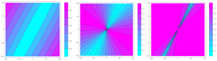
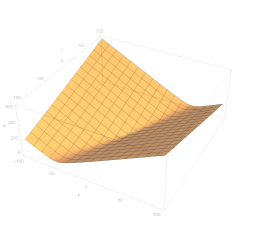
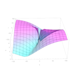
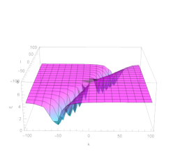
$\omega$ $v_{f}$ $v_{g}$

Figure 1: In these graphics we represent the dispersion relation, phase speed and group speed for a choice of parameters $R_{9}=1$, $R_{10}=2$, $m_{1}=n_{1}=n_{2}=1$, $m_{2}=2$ . In the top pictures we represent them in 2D and in the bottom the same quantities in 3D, since both complement visually the description. In the left column we observe dispersion relation $\omega(k,l)$ (Top contour plot and bottom as 3D plot), the central column represents those values for the phase speed. The right column corresponds to the group speed.

In figure 1, (Figure 1), we show the values of the phase and group speed of the dispersion relation. We can observe that while the group speed is constant the phase one varies. For the following $R_{9}=1$,$R_{10}=2$, $m_{1}=n_{1}=n_{2}=1$, $m_{2}=2$, and assuming for illustrative purposes $k,l$ as real variables.

When we impose the group velocity and the phase speed to be equal, generically the system exhibit dispersion. However, it also admits solutions without dispersion and non vanishing central charge. For example, for a choice of $j=n_{r}/m_{r}$ with a fixed $r$, and winding charges $m_{r}=m_{s};n_{r}=-n_{s}$ with $r\neq s$ the two velocities coincide and the system does not exhibit dispersion. There are other more particular winding charge configurations that also satisfy the identity of velocities for the $j$ considered, like for example $n_{1}=3,m_{1}=4,n=2=12,m_{2}=16$ with non-vanishing central charge.

Second family of solutions

We are interested in allowing a more general dependence on time of the real scalar fields $A_{r}$, such that the symplectic gauge field, $\mathbb{A}$ with contain a generic field strength $\mathcal{F}$. To this end, we assume the following ansatz

$$Z_{a}=\left(\sin(\lambda(k\sigma+l\rho))+\cos(\lambda(k\sigma+l\rho))\right)a_{a}e^{i\tau\omega}\,,$$ (51)

$$A_{r}=a_{r}\left(a\sin(\lambda(k\sigma+l\rho)+\tau\Omega)+b\cos(\lambda(k\sigma+l\rho)+\tau\Omega)\right)\,.$$ (52)

Proceeding as before, we obtain from the EOM for $Z$, the frequency $\omega$ is not modified in spite of the modification of the $A_{r}$ ansatz. This is due to the fact that in the isotropic case considered in this section, both EOM decouple. It is given by

$$\omega^{2}=\lambda^{2}\sum_{r}R_{r}^{2}\left(km_{r}-ln_{r}\right)^{2}\,,$$ (53)

and from the EOM for $A_{r}$, one obtains two frequency $\Omega$. It depends on the moduli of the torus, the winding numbers and the amplitudes of the $A_{r}$ field,

$$\Omega^{2}=\lambda^{2}\left(\left(km_{s}-ln_{s}\right)^{2}R_{s}^{2}-\frac{a_{s}}{a_{r}}\left(km_{r}-ln_{r}\right)\left(km_{s}-ln_{s}\right)R_{r}R_{s}\right)\,,$$ (54)

with $r\neq s,r=1,2$. In distinction with the previous case analyzed, the APD constraint is not automatically satisfied and leaves the following restriction,

$$a_{r}R_{r}\left(km_{r}-ln_{r}\right)+a_{s}R_{s}\left(km_{s}-ln_{s}\right)=0\,.$$ (55)

The constraint can be used to fix the relation $a=a_{s}/a_{s}$. Imposing the constraint in (54) the frequency $\Omega$ becomes

$$\Omega^{2}=2\lambda^{2}R_{s}^{2}\left(km_{s}-ln_{s}\right)^{2}\,,$$ (56)

for $s$ fixed. By imposing the constraint on (53),

$$\omega^{2}=\lambda^{2}R_{s}^{2}\left(km_{s}-ln_{s}\right)^{2}(1+a^{2})\,,$$ (57)

with no sum is intended. Due to the APD constraint and for this particular ansatz, both frequencies become related by,

$$\Omega^{2}=\frac{2\omega^{2}}{1+a^{2}}\,,$$ (58)

As an illustrative example let us consider the case with $a=1$. It implies that the two components of the $A_{r}$ become equal and that $\Omega=\omega$. In distinction with the first family case, the relation between the Fourier modes $j=k/l$ gets restricted by the APD constraint to a unique value, for a fixed moduli and winding charges, that in this case corresponds to

$$j=k/l=\frac{(R_{r}n_{r}+R_{s}n_{s})}{(R_{r}m_{r}+R_{s}m_{s})}\,.$$ (59)

The integer character of the Fourier modes force, on general grounds, the radii to be integer. For a given moduli and winding charges, i.e. if the topological content is fixed, then only a unique relation of Fourier modes $j$ is allowed.

Now, we want to characterize their dispersion. The velocity group associated to the dispersion relation has a constant magnitude

$$\textbf{v}_{g}=\frac{\partial\omega}{\partial\textbf{k}}\equiv\lambda R_{r}\sqrt{2}\left(m_{r}\ ,-\ n_{r}\right);\quad\Rightarrow\quad|\textbf{v}_{g}|=\sqrt{2}\lambda R_{r}\sqrt{\left(m_{r}^{2}+n_{r}^{2}\right)}\ .$$ (60)

for $r$ fixed.

With respect to the dispersion, we observe the following, Their phase speed is given by

$$c(\textbf{k}) =\sqrt{2}\lambda R_{r}\frac{\left(km_{r}-ln_{r}\right)}{\sqrt{k^{2}+l^{2}}}\,.$$ (61)

It is straightforward to see, that their phase speed along each of the directions verify $jc_{\sigma}=c_{\rho}$. We can observe that although the system presents generically dispersion, there exists areas which are dispersion-free. In order to see if there exists points in the phase space moduli free of dispersion, we impose $c(\textbf{k})=|\textbf{v}_{g}|,$

$$(km_{r}-ln_{r})=\sqrt{k^{2}+l^{2}}\sqrt{\left(m_{r}^{2}+n_{r}^{2}\right)}\,,$$ (62)

which implies,

$$l=-\frac{n_{r}}{m_{r}}k\ .$$ (63)

for $r$ fixed. Hence, for central charge different from zero the system in general exhibits dispersion but it also allows solutions with no dispersion satisfying (63).

Before concluding this section, some remarks are in order,

In first place, we obtain for the isotropic case that, in spite of the non-linearities of the system, when the symplectic field $\mathbb{A}$ and the complex scalar field $Z$ become determined in terms of the same real single function $f(\sigma,\rho)$, the system is strongly simplified and it admits solutions of sinusoidal type. In Section 5, we will analyze the superposition of these types of solutions and see that their superposition is strongly restricted due to the fact that the are solutions to the nonlinear equations of motion.

Secondly, we could have focused from the very beginning on a subfamily of solutions given by $\partial^{2}f\propto f$. This solution subfamily corresponds to the $\lambda=1$ choice. The main constraints on this first family of solutions are imposed by the periodicity condition required since they propagate on the world volume of a compact membrane. Solving this system of equations on a flat plane would admit much more general solutions for the given ansatz.

Third, the second family of solutions allows for a nontrivial time dependence for $A_{r}$, resulting in a general symplectic curvature $\mathcal{F}$. Under the ansatz considered, the frequencies of the $A_{r}$ and Q-ball solutions become related, and for $a=1$, both determine a unique excitation for a pair $(k,l)$. In this case, for a given moduli, there exists a single pair of Fourier modes for each set of winding numbers with a given central charge. The APD constraint represents the main restriction to the allowed solutions.

Both families of solutions to the nonlinear system of EOM exhibit generically dispersion although in both cases, they also admit solutions without dispersion with a non-vanishing central charge.

4 Superposition of solutions: Vectorization

An important aspect of solitonic solution is the fact that on very general grounds, solitons cannot be superposed linearly. In fact, this is a characteristic property, however, there are some exceptions, that for a restricted range of frequencies, admit linear superpositions like it is the case for optical solitons, SuperpositionsBrightanddarksolitons ; LinearSuperpositionPonomarenko2002 ; ZHOU20171697:LinearSuperpositionPrinciple . We show in this section that this is also the case of the Q-ball-like solutions analyzed in section 3. We will see that in the absence of a symplectic gauge field, we are able to obtain multi-soliton solutions that naively seems to corresponds to a linear superposition but restricted to a very specific discrete set of frequencies given by the monopole contribution. In order to understand it better we will do it in several steps.

4.1 Fourier series solution

Although we are interested in Q-ball-like solutions, we will start by analyzing the behaviour of the EOM of the M2-branes with worldvolume fluxes for the case of a superposition of the complexified analytic solutions found previously in section 3. We can observe that they correspond to a Fourier serie. Since this is a sum, with matrix entries, it is not automatically guaranteed that the superposition of solutions will be also a solution due to the non-linearities of the differential equations. Indeed we are interested in finding the conditions under which this may happen. Let us consider $f_{a}(\sigma,\rho)$ represented by a Fourier series:

$$f_{a}^{\mathbb{C}}=\sum_{k,l=0}^{\infty}a_{kl}f^{kl}_{a}(\sigma,\rho)\,.$$ (64)

The $kl$-th element of the orthogonal basis is given by:

$$f^{kl}_{a}(\sigma,\rho)=\cos(k\sigma+l\rho)+i\sin(k\sigma+l\rho)\,.$$ (65)

It is easy to verify that, with a proper normalization:

$$\int_{0}^{2\pi}\int_{0}^{2\pi}f^{kl}_{a}(\sigma,\rho)~{}f^{uv}_{a}(\sigma,\rho)~{}d\sigma~{}d\rho=\begin{cases}0&uv\neq kl\\ 1&uv=kl\end{cases}$$ (66)

with,

$$a_{nm}=\int_{0}^{2\pi}\int_{0}^{2\pi}f_{a}(\sigma,\rho)~{}f^{kl}_{a}(\sigma,\rho)~{}d\sigma d\rho\,.$$ (67)

Imposing smoothness on $f$ and differentiability term-by-term, see for example section $3.4$ in Haberman . The series (64) can be written as:

$$f_{a}^{\mathbb{C}}=\sum_{\xi_{u}=0}^{\infty}a_{\xi_{u}}e^{i~{}\xi_{u}.u}\,,$$ (68)

and derivatives

$$\partial_{u}f_{a}(u)=\sum_{\xi_{u}=0}^{\infty}a_{\xi_{u}}i~{}\xi_{u}~{}e^{i~{}\xi_{u}.u},\ \ \partial_{u}^{2}f_{a}(\sigma,\rho),=-\sum_{\xi_{u}=0}^{\infty}a_{\xi_{u}}\xi_{u}^{2}~{}e^{i\xi_{u}u},\ \ \partial_{uv}^{2}f_{a}(\xi_{u})=-\sum_{\xi_{u}=0}^{\infty}a_{\xi_{u}}\xi_{u}\xi_{v}~{}e^{i~{}\xi_{u}u},$$ (69)

with $u\not=v$. We have defined the vector $u=(\sigma,\rho)$ labeling the spatial coordinates and the vector $\xi_{u}=(k,l)$ labeling the Fourier modes of the expansion, and $a_{xi_{u}}$ the constant amplitude of $f_{a}^{\mathbb{C}}$.

To implement the expansion numerically, we use a truncated version of the series (64) and define, the vectors:

$${\bf k} = \left(0,1,2,3,\cdots N,1,2,3,\cdots,N,\cdots\right)\,,$$

$${\bf l} = \left(0,0,0,0,\cdots 1,1,1,1,\cdots,N,N,N,\cdots\right),$$

$${\bf k}^{2} = \left(0,1,4,9,\cdots,k^{2},\cdots N^{2}\right),$$

$${\bf l}^{2} = \left(0,0,0,0,\cdots,l^{2},\cdots N^{2}\right),$$

$${\bf kl} = \left(0,0,0,0;0,1,2,3,\dots;0,2,4,6,\cdots,kl,\cdots,\right),$$

$${\bf f}_{a}(\sigma,\rho) = \left(a_{11}~{}f_{a}^{11}(\sigma,\rho),a_{12}~{}f_{a}^{12}(\sigma,\rho),\cdots,a_{1N}~{}f_{a}^{1N}(\sigma,\rho),a_{21}~{}f_{a}^{21}\cdots,a_{NN}~{}f_{a}^{NN}\right),$$

$$\mathbf{\omega}^{2} = \left(\omega_{11},\omega_{12},\omega_{13},\cdots,\omega_{kl},\cdots,\omega_{NN}\right).$$ (70)

See also that ${\bf l}$ must be defined in a different way than the others indices. With the above notation defined and considering only $Sine$ or $Cosine$ series, we can write:

$$\partial_{\sigma}f_{a}(\sigma,\rho) = i~{}{\bf k}\cdot\textbf{f}_{a}(\sigma,\rho),\quad\partial_{\rho}f_{a}(\sigma,\rho)=i~{}{\bf l}\cdot\textbf{f}(\sigma,\rho),$$

$$\partial_{\sigma}^{2}f_{a}(\sigma,\rho), = -{\bf k}^{2}\cdot\textbf{f}(\sigma,\rho),\quad\partial_{\rho}^{2}f_{a}(\sigma,\rho)=-{\bf l}^{2}\cdot\textbf{f}(\sigma,\rho),$$

$$\partial^{2}_{\sigma\rho}f_{a}(\sigma,\rho) = -{\bf kl}\cdot\textbf{f}(\sigma,\rho),$$ (71)

where, $(\cdot)$ denotes a inner product. See that obviously this is not a general property but a property of the Lie bracket and the base chosen that we know that satisfies the equations in the case of a single solution. The Figure (2) compares in a graphic fashion, the "analytic" derivative and "inner product version" of the derivative in the case of $\partial^{2}_{\sigma\rho}f_{a}(\sigma,\rho)$. See that the agreement is very good.

Figure 2: The Figure of left represents the analytic derivative behaviour and the Figure of the right "inner product version" of the derivative in the case of $\partial^{2}_{\sigma\rho}f_{a}(\sigma,\rho)$. As we can observe both graphics are indistinguibles.

The system that we intend to solve corresponds to the EOM (2) and (2) with $A_{r}=constant$

$$-C_{1}\left(\partial_{\sigma}^{2}f_{a}\right)+2~{}C_{2}\left(\partial^{2}_{\sigma\rho}f_{a}\right)-C_{3}\partial_{\rho}^{2}f_{a}=\omega^{2}f_{a},$$ (72)

$$\left(m_{r}\partial_{\sigma}^{2}f_{a}-n_{r}\partial^{2}_{\sigma\rho}f_{a}\right)\partial_{\rho}f_{a}-\left(m_{r}\partial^{2}_{\rho\sigma}f_{a}-n_{r}\partial_{\rho}^{2}f_{a}\right)\partial_{\sigma}f_{a}=0\,,$$ (73)

where $C_{1}=m_{9}^{2}R_{9}^{2}+m_{10}^{2}R_{10}^{2}$, $C_{2}=m_{9}n_{9}R_{9}^{2}+n_{10}m_{10}R_{10}^{2}$, $C_{3}=n_{9}^{2}R_{9}^{2}+n_{10}^{2}R_{10}^{2},$ with $r=9,10$, $n_{r},m_{r}$, the winding numbers, $R_{r}$ the torus radii and $\omega\in\mathbb{R}$. The APD constraint is identically verified. It is subject to the central charge condition (24).

We impose now the ansatz of the family (25) for the isotropic case. The equation (72) written in the inner product version results in:

$$\left(C_{1}~{}{\bf k}^{2}-2~{}C_{2}~{}{\bf kl}+C_{3}{\bf l}^{2}\right)\cdot\textbf{f}(\sigma,\rho) = \mathbf{\omega}^{2}\cdot\textbf{f}(\sigma,\rho),$$ (74)

where each component, it can be expressed directly in terms of their breathing modes:

$$C_{1}~{}k^{2}-2~{}C_{2}~{}kl+C_{3}~{}l^{2}=\omega_{kl}^{2}\,.$$ (75)

The second equation (73), since it contains the nonlinearities is more involved, but still can be expressed in this simple algebraic way:

$$-[\left(m_{r}{\bf k}^{2}-n_{r}{\bf kl}\right)\cdot\mathbf{f}(\sigma,\rho)]\times[~{}{\bf l}\cdot\textbf{f}(\sigma,\rho)]+[\left(m_{r}{\bf kl}-n_{r}{\bf l}^{2}\right)\cdot\mathbf{f}(\sigma,\rho)]\times[~{}{\bf k}\cdot\textbf{f}(\sigma,\rho)]=0.$$ (76)

Here $\times$ represents the product between scalars or scalar and vectors. In order to solve this equation, let us define the vectors:

$${\boldsymbol{\alpha}}_{r}=m_{r}{\bf k}^{2}-n_{r}{\bf kl},\quad{\boldsymbol{\beta}}_{r}=m_{r}{\bf kl}-n_{r}{\bf l}^{2}\,,$$ (77)

with components $\alpha_{m}$ and $\beta_{m}$, respectively, and being ${\bf f}_{mn}$ represents the matrix elements of ${\bf f}$. The equation (76) expressed in terms of $\boldsymbol{\alpha},\boldsymbol{\beta}$ becomes

$$-(\boldsymbol{\alpha}_{r}\cdot\mathbf{f}(\sigma,\rho))\times({\bf l}\cdot\textbf{f}(\sigma,\rho))+(\boldsymbol{\beta}_{r}\cdot\mathbf{f}(\sigma,\rho))\times({\bf k}\cdot\textbf{f}(\sigma,\rho))=0\,.$$ (78)

Before continuing, it is interesting to note that if the series (64) has only one term, the equation (73) is identically satisfied, since,

$$n_{r}~{}l^{2}~{}k-m_{r}~{}l~{}k^{2}+m_{r}~{}l~{}k^{2}-n_{r}~{}kl^{2} = 0\,,$$ (79)

which agrees with the results of Section 3. therefore, The eigenvalues and eigenvectors obtained between the analytical and numerical methods are very similar to those found in SpinningSolutionsBosonicM2-brane2022 although in that case they were numerical solutions to the approximate system, (i.e. without considering the restriction of (73)). This means that the simplest solutions obtained is in the kernel of the monopole restriction.

4.2 Solving an algebraic problem

In order to find a larger set of solutions, we have transformed our initial problem into another one: find a $\bf f$ that fulfill (78). Since (78) can be written as,

$$\left[-\boldsymbol{\alpha}_{r}\cdot\mathbf{f}(\sigma,\rho)\times~{}{\bf l}+\boldsymbol{\beta}_{r}\cdot\mathbf{f}(\sigma,\rho)\times~{}{\bf k}\right]\cdot\textbf{f}(\sigma,\rho)=0.$$ (80)

There are two alternatives: one can linearly transform $\bf f$ (selecting the set of coefficients $a_{mn}$), so that obtain a vector

$$-\boldsymbol{\alpha}_{r}\cdot\mathbf{f}(\sigma,\rho)\times~{}{\bf l}+\boldsymbol{\beta}_{r}\cdot\mathbf{f}(\sigma,\rho)\times~{}{\bf k},$$ (81)

orthogonal to $\bf f$ (this seems to be an interesting, but complicated problem), or more easily, we can suppose that ${\bf f}\neq 0$, and find ${\bf f}$ (the set of coefficients $a_{mn}$ that satisfy the equation), that is:

$$\boldsymbol{\alpha}_{r}\cdot\mathbf{f}(\sigma,\rho)\times~{}{\bf l}=\boldsymbol{\beta}_{r}\cdot\mathbf{f}(\sigma,\rho)\times~{}{\bf k}\,.$$ (82)

In order to find a solution to ((73)), we denote the position of an element by $l_{j}$, in the corresponding vector, say for example ${\bf{l}}$. Then the solution with the allowed values is found when $k_{j}=l_{j}$ for $j=i+(i-1)N$ being $N$ the order of the truncation and $i$ the position inside it, $i=1,\dots,N$. The coefficient values in those positions are given by $l_{j}=k_{j}=i-1$. The solution then arises for the subfamily of functions $f^{\mathbb{C}}$ with $a_{k_{j}l_{j}}=1$ and zero otherwise. It corresponds to the diagonal terms of f in a matrix representation.

Hence, we obtain that the superposition of arbitrary functions with equal Fourier modes is solution to the EOM (72) and (73) whenever those modes are equal. This condition, constrains the set of solutions of equation (72), and reflects the nonlinearity in behavior to the equation (73), associated with the presence of a monopole solution constructed in terms of the $\widehat{X}_{r}$.

In short, a general solution for the EOM (72) and (73) system with a QBL ansatz and nonvanishing central charge can be written in terms of the real parts of $f^{\mathbb{C}}$. It is straightforward to see that the same result holds for

$$f_{a}(\sigma,\rho,w)=\sum_{k=1}^{M}a_{kk}\left[\cos(k(\rho+\sigma))+\sin(k(\rho+\sigma)\right]\,.$$ (83)

The sum runs over the number of pairs $M$ that fulfill the solution. It represents a Q-ball-like multisoliton solution for the isotropic case with a non vanishing central charge.

In summary, the analytic family of QBL solutions for the isotropic case and constant gauge field and with central charge different from zero admit a linear superposition law but only when the frequencies become strongly constrained to be equal. We emphasize that this is not true otherwise. All of these case require a central charge different from zero -which we recall it is associated to the presence of a magnetic monopole over the worldvolume MARTINRestucciaTorrealba1998:StabilityM2Compactified . This represents the superposition law for this type of solutions.

In the following we illustrate an example of superposition of solutions.

Here, it can be seen how the proposed solution complies with the equation (72-73), with $\{k_{j},l_{j}\}_{j=0}^{M}=\{\{0,0\},\{1,1\},\{2,2\},\{3,3\},\{4,4\}\}$ and $m_{9}=9$, $m_{10}=2$, $n_{9}=9$, $n_{10}=8$, $R_{9}=1$ and $R_{10}=11$ with non-vanishing central charge.

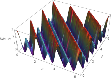
Figure 3: Analytic solution of (72)-(73)

We observe the following: i) The equation (78), is very interesting since it allows to reduce the order of non-linearity in this type of equations, ii) The condition (73) seems to act as a pruning to the basis (solutions) generated by the eigenvalue (72) ad iii) The linear superposition is not possible on general grounds due to the nonlinearities of the equation (73). However, it can be obtained when the values of the Fourier modes becomes strongly constrained to specific pairs that determine the frequencies due to the nonlinear behaviour of (73). There are in the literature other examples of nonlinear EPD that admit restricted linear superposition, see Han2022 .

5 Numerical solutions to the Q-ball

We analyze two different cases. This can be also compared with the analytical one. In second place we obtain the non-isotropic case. Both analysis are performed when no symplectic gauge field is present, i.e. for $A_{r}$ constant or with a linear dependence only on $\tau$.

5.1 Q-ball solution: The isotropic case

For the isotropic case and constant $A_{r}$ we consider the system of equations given by (72) and (73) subject to the central charge condition 3 discussed in section 4. The Q-ball ansatz automatically satisfy the Area preserving constraint. The solutions of the equation (72) was analyzed in SpinningSolutionsBosonicM2-brane2022 and a discrete set of frequencies was obtained. From a numerical point of view the M2-brane system of partial differential equations that we consider is: i) Overdetermined. In the sense that the unknown function must satisfy two different differential equations ii) Nonlinear. Although only to the second equation, where in this case the non-linearities are represented by products of different derivatives (in order and variable) of the unknown function and iii)Rare. The most striking feature is that this form of nonlinearity is unusual and, as far to our knowledge, there are no reported numerical methods for solving it. Neither in the finite dimensional (ODEs) or infinite dimensional (PDEs) case.

The three steps algorithm we will follow in order to a find numerical solution to the (72-73) system will be

• Set the boundary condition. In principle boundary ($\Gamma$) condition can be fixed as: Dirichlet or Periodic, though in this case we will restrict to periodic boundary conditions on $\Gamma$:

  $$f(0,\rho)=f(2\pi,\rho),\quad f(\sigma,0)=f(\sigma,2\pi)\,.$$ (84)

• Solve (72 ) as an eigenvalue problem:

  $${\cal L}_{p}\varphi_{n}(\sigma,\rho)=\omega_{n}~{}\varphi_{n}(\sigma,\rho).$$ (85)

• Write the solution of (73) as

  $$f_{a}(\sigma,\rho)=\sum_{n=0}^{\infty}\gamma_{n}\varphi_{n}(\sigma,\rho).$$ (86)

  and solve an optimization problem to find the best set of $\gamma_{n}$, so that (86) is solution of (73).

5.1.1 Finite differences approach for the solution

The system (72)-(73) can be re-written using centered Euler scheme:

$${\cal D}_{\sigma}\varphi_{n}=\frac{\varphi_{n}^{i+1,j}-\varphi_{n}^{i-1,j}}{2\Delta\sigma},\quad{\cal D}_{\rho}\varphi_{n}=\frac{\varphi_{n}^{i,j+1}-\varphi_{n}^{i,j-1}}{2\Delta\rho},$$ (87)

$${\cal D}^{2}_{\sigma}\varphi_{n}=\frac{\varphi_{n}^{i+1,j}-2\varphi_{n}^{i,j}+\varphi_{n}^{i-1,j}}{\Delta\sigma^{2}},\quad{\cal D}^{2}_{\rho}\varphi_{n}=\frac{\varphi_{n}^{i,j+1}-2\varphi_{n}^{i,j}+\varphi_{n}^{i,j-1}}{\Delta\rho^{2}},\quad$$ (88)

with the mixed second derivative given:

$${\cal D}^{2}_{\sigma,\rho}\varphi_{n}=\frac{\varphi_{n}^{i+1,j+1}-\varphi_{n}^{i-1,j+1}-\varphi_{n}^{i+1,j-1}+\varphi_{n}^{i-1,j-1}}{4\Delta\sigma\Delta\rho}$$ (89)

It is easy to verify that:

$${\cal D}_{\rho}\approx{\partial}_{\rho},\quad{\cal D}_{\sigma}\approx{\partial}_{\sigma}.\quad{\cal D}^{2}_{\sigma}\approx{\partial}^{2}_{\sigma},\quad{\cal D}^{2}_{\sigma,\rho}\approx{\partial}^{2}_{\sigma,\rho},\quad{\cal D}^{2}_{\rho}\approx{\partial}^{2}_{\rho}\,.$$ (90)

Since equation (72) is linear, it can be solved relatively easily using finite differences or built-in functions from Mathematica or Python. In the case of the second equation we must use a different methodology due to its intrinsic nonlinearities.

5.1.2 A finite differences representation for the nonlinear equation

Re-writing the equation (73) in terms of finite differences become,

$$\left(m_{r}\partial_{\sigma}^{2}\sum_{n=0}^{\infty}\gamma_{n}\varphi_{n}(\sigma,\rho)-n_{r}\partial^{2}_{\sigma\rho}\sum_{n=0}^{\infty}\gamma_{n}\varphi_{n}(\sigma,\rho)\right)\partial_{\rho}\sum_{n=0}^{\infty}\gamma_{n}\varphi_{n}(\sigma,\rho) -$$

$$\left(m_{r}\partial^{2}_{\rho\sigma}\sum_{n=0}^{\infty}\gamma_{n}\varphi_{n}(\sigma,\rho)-n_{r}\partial_{\rho}^{2}\sum_{n=0}^{\infty}\gamma_{n}\varphi_{n}(\sigma,\rho)\right)\partial_{\sigma}\sum_{n=0}^{\infty}\gamma_{n}\varphi_{n}(\sigma,\rho) = 0.$$ (91)

$$\left(m_{r}\sum_{n=0}^{\infty}\gamma_{n}\partial_{\sigma}^{2}\varphi_{n}(\sigma,\rho)-n_{r}\sum_{n=0}^{\infty}\gamma_{n}\partial^{2}_{\sigma\rho}\varphi_{n}(\sigma,\rho)\right)\sum_{n=0}^{\infty}\gamma_{n}\partial_{\rho}\varphi_{n}(\sigma,\rho) -$$

$$\left(m_{r}\sum_{n=0}^{\infty}\gamma_{n}\partial^{2}_{\rho\sigma}\varphi_{n}(\sigma,\rho)-n_{r}\sum_{n=0}^{\infty}\gamma_{n}\partial_{\rho}^{2}\varphi_{n}(\sigma,\rho)\right)\sum_{n=0}^{\infty}\gamma_{n}\partial_{\sigma}\varphi_{n}(\sigma,\rho) = 0.$$ (92)

$$\left[\sum_{n=0}^{\infty}\gamma_{n}\left(m_{r}\partial_{\sigma}^{2}\varphi_{n}(\sigma,\rho)-n_{r}\partial^{2}_{\sigma\rho}\varphi_{n}(\sigma,\rho)\right)\right].\sum_{n=0}^{\infty}\gamma_{n}\partial_{\rho}\varphi_{n}(\sigma,\rho) -$$

$$\left[\sum_{n=0}^{\infty}\gamma_{n}\left(m_{r}\partial^{2}_{\rho\sigma}\varphi_{n}(\sigma,\rho)-n_{r}\partial_{\rho}^{2}\varphi_{n}(\sigma,\rho)\right)\right].\sum_{n=0}^{\infty}\gamma_{n}\partial_{\sigma}\varphi_{n}(\sigma,\rho) = 0.$$ (93)

This can be re-expressed in a more compact form as:

$$\sum_{n=0}^{\infty}\gamma_{n}\left(A_{n}-B_{n}\right)\cdot\sum_{n=0}^{\infty}\omega_{n}C_{n}-\sum_{n=0}^{\infty}\gamma_{n}\left(B_{n}-D_{n}\right)\cdot\sum_{n=0}^{\infty}\omega_{n}E_{n} = 0.$$ (94)

where:

$$A_{n}=m_{r}\partial_{\sigma}^{2}\varphi_{n}(\sigma,\rho),\quad B_{n}=n_{r}\partial^{2}_{\sigma\rho}\varphi_{n}(\sigma,\rho),\quad C_{n}=\partial_{\rho}\varphi_{n}(\sigma,\rho),$$ (95)

and

$$D_{n}=\partial_{\rho}^{2}\varphi_{n}(\sigma,\rho),\quad E_{n}=\partial_{\sigma}\varphi_{n}(\sigma,\rho)\,.$$ (96)

Using the Cauchy product in (94), we obtain:

$$\sum_{n=0}^{\infty}\sum_{m=0}^{n}\gamma_{n}\left(A_{n}-B_{n}\right)~{}\odot\gamma_{n-m}C_{n-m}-\sum_{n=0}^{\infty}\sum_{m=0}^{n}\gamma_{n}\left(B_{n}-D_{n}\right)~{}\odot\gamma_{n-m}E_{n-m}=0\,.$$ (97)

$$\sum_{n=0}^{\infty}~{}\gamma_{n}\left(\sum_{m=0}^{n}\gamma_{n-m}S_{n,m}\right)=0,$$ (98)

with,

$$S_{n,m}=\left(A_{n}-B_{n}\right)\odot C_{n-m}-\left(B_{n}-D_{n}\right)\odot E_{n-m}\,,$$ (99)

and $\odot$ represents the pointwise product. Thus, the solution of the problem can be reduced to find a solution for this nonlinear algebraic equation with matrix coefficients and $\gamma_{n}$ as unknowns.

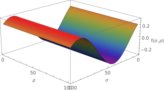
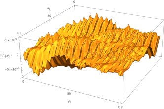
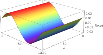
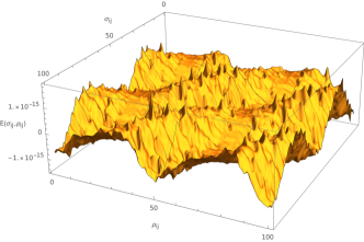
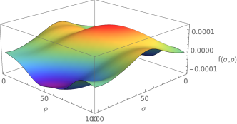
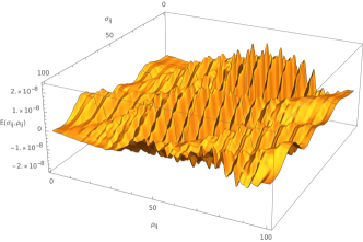
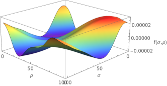
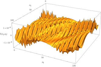
Figure 4: Approximate solution of (72)-(73) and error of approximation.

We define the error function in the following way,

$$E(\rho_{ij},\sigma_{ij}) = \left(m_{r}\partial_{\sigma}^{2}f_{a}(\rho_{ij},\sigma_{ij})-n_{r}\partial^{2}_{\sigma\rho}f_{a}(\rho_{ij},\sigma_{ij})\right)\partial_{\rho}f_{a}(\rho_{ij},\sigma_{ij})-$$ (100)

$$\left(m_{r}\partial^{2}_{\rho\sigma}f_{a}(\rho_{ij},\sigma_{ij})-n_{r}\partial_{\rho}^{2}f_{a}(\rho_{ij},\sigma_{ij})\right)\partial_{\sigma}f_{a}(\rho_{ij},\sigma_{ij})\,.$$

Figure 4 shows graphs of the possible solutions (note that the numerical scheme allows for many, unless the number of bases equals the number of lattices squared) and the errors made in those approximations at each lattice point.

We obtain two kinds of solutions: some with large amplitudes and others with small amplitudes. This may be because the parameters $n$, $m$, and $R$ may be in very different ranges.

5.2 Q-ball solution: Non-isotropic case

In section 3. we have obtained the first exact analytical families of solutions for a Q-ball ansatz of the complex scalar field. They correspond to isotropic solutions and with the nonlinear behaviour encoded in the $A_{r}$ field which is expressed in terms of $f$, and hence makes the complex scalar field $Z$ to be nontrivial. However, the family of solutions ob tained trivializes the non-isotropic contribution of the brackets to the $Z$ EOM. In order to capture their contribution, in this section we consider the non-isotropic case in the absence of a symplectic gauge field $\mathbb{A}$.

Imposing $A_{r}=Constant$ in the E.O.M (28) they become the following nonlinear but simplified system of equations:

$$\omega_{c}^{2}f_{c}=-\sum_{r=9}^{10}\left[R_{r}(j_{c}m_{r}-n_{r})\right]^{2}\partial_{\rho}^{2}f_{c}-\sum_{a}(j_{c}-j_{a})^{2}\partial_{\rho}^{2}f_{c}(\partial_{\rho}f_{a})^{2}\ .$$ (101)

with $a,c=1,2,3$ and $r,s=1,2$. In order to simplify the notation, let us define the constants $\kappa_{a}$,

$$\kappa_{a}=\sum_{r=9}^{10}\left[R_{r}(j_{a}m_{r}-n_{r})\right]^{2}\,,$$ (102)

in addition to the matrices $\lambda$ and $\mu$, with elements:

$$\lambda_{c,a}=(j_{c}-j_{a})^{2},\qquad\mu_{r,a}=\left[R_{r}\left(j_{a}m_{r}-n_{r}\right)\right]^{2}\,,$$ (103)

with $r$, $c$ y $a$, defined as before. With this notation, the above equations can be written as:

$$-\kappa_{1}~{}\partial_{\rho}^{2}f_{1}-\partial_{\rho}^{2}f_{1}~{}\sum_{a}\lambda_{1,a}(\partial_{\rho}f_{a})^{2} = \omega_{1}^{2}f_{1}\,,$$

$$-\kappa_{2}~{}\partial_{\rho}^{2}f_{2}-\partial_{\rho}^{2}f_{2}~{}\sum_{a}\lambda_{2,a}(\partial_{\rho}f_{a})^{2} = \omega_{2}^{2}f_{2}\,,$$

$$-\kappa_{3}~{}\partial_{\rho}^{2}f_{3}-\partial_{\rho}^{2}f_{3}~{}\sum_{a}\lambda_{3,a}(\partial_{\rho}f_{a})^{2} = \omega_{3}^{2}f_{3}\,.$$ (104)

5.2.1 A numerical approach to the solution

In order to write our problem in a convenient way for its numerical integration, $x^{\prime}={\mathbf{f}}(x)$ con $x\in\Re^{3}$, let’s start by defining $\partial_{\rho}f_{a}=g_{a}$, so that the equations (101) can be written as:

$$\partial_{\rho}f_{1}=g_{1};\qquad-\kappa_{11}~{}\partial_{\rho}g_{1}-\partial_{\rho}g_{1}~{}\sum_{a}\lambda_{1,a}g_{a}^{2}=\omega_{1}^{2}f_{1}\,,$$

$$\partial_{\rho}f_{2}=g_{2};\qquad-\kappa_{22}~{}\partial_{\rho}g_{2}-\partial_{\rho}g_{2}~{}\sum_{a}\lambda_{2,a}g_{a}^{2}=\omega_{2}^{2}f_{2}\,,$$

$$\partial_{\rho}f_{3}=g_{3};\qquad-\kappa_{33}~{}\partial_{\rho}g_{3}-\partial_{\rho}g_{3}~{}\sum_{a}\lambda_{3,a}g_{a}^{2}=\omega_{3}^{2}f_{3}\,.$$ (105)

So, if we include the boundary conditions, our problem will look like:

$$\partial_{\rho}f_{b}=g_{b};\qquad\partial_{\rho}g_{b}=\frac{\omega_{b}^{2}f_{b}}{\kappa_{bb}~{}+~{}\sum_{a}\lambda_{b,a}g_{a}^{2}}\,,$$ (106)

with $f_{i}(0)=f_{i}(2\pi)\quad i=1,2,3$. Thus, our problem is to find a function:

$$x(\rho)=(f_{1}(\rho),g_{1}(\rho),f_{2}(\rho),g_{2}(\rho),f_{3}(\rho),g_{3}(\rho)),$$ (107)

that satisfies:

$$\frac{\partial x(\rho)}{\partial\rho}={\mathbf{f}}(x)\,,$$ (108)

where ${\mathbf{f}}$ is a vector-valued function given by:

$${\mathbf{f}}(x)=\left(\begin{array}[]{c}g_{1}(\rho)\\ \\ \frac{\omega_{1}^{2}f_{1}(\rho)}{\kappa_{1}~{}+~{}\sum_{a}\lambda_{1,a}g_{a}^{2}(\rho)}\\ \\ g_{2}(\rho)\\ \\ \frac{\omega_{2}^{2}f_{2}(\rho)}{\kappa_{2}~{}+~{}\sum_{a}\lambda_{2,a}g_{a}^{2}(\rho)}\\ \\ g_{3}(\rho)\\ \\ \frac{\omega_{3}^{2}f_{3}(\rho)}{\kappa_{3}~{}+~{}\sum_{a}\lambda_{3,a}g_{a}^{2}(\rho)}\end{array}\right),$$ (109)

with the boundary condition $x(0)=x(2\pi)$.

5.2.2 The proposed solution

Since this problem can be assimilated to the class of "two point boundary value problems", we propose to use a customized version of the "shooting method", to obtain numerical solutions. In these methods, since only part of the initial condition ($f_{i}(0)$) is known, the remaining part is assumed to be known and the initial value problem is solved, varying this last part, until the solution complies with the remaining boundary condition.

A more or less efficient way to implement this idea, is to find the roots ($g_{1}^{*},g_{2}^{*},g_{3}^{*}$) of the function:

$$F(x(0),\rho)=\Phi(x(0),2\pi)-x(2\pi)\,,$$ (110)

where $\Phi(x(0),\rho)$ is the solution of the initial value problem:

$$\frac{\partial x(\rho)}{\partial\rho}={\mathbf{f}}(x)\,,$$ (111)

with initial conditions $x(0)=(f_{1}(0),g_{1}(0),f_{2}(0),g_{2}(0),f_{3}(0),g_{3}(0))$.

The most popular way to solve the problem (110), is using Newton’s method. This type of methods can be extended to the case of problems of the type that concern us ("two point boundary values") in many ways. One of them, given in Aprille , states that:

$$x^{i+1}(0)=x^{i}(0)+(J_{\Phi}-I)^{-1}\left[\Phi(x^{i}(0),2\pi)-x^{i}(0)\right]\,,$$ (112)

where $J_{\Phi}$ is the derivative of the solution ($\Phi$) evaluated $2\pi$, also called "sensitivity matrix",

$$J_{\Phi}=\frac{\partial\Phi(x(0),2\pi)}{\partial x(0)}|_{x^{i}(0)}\,.$$ (113)

and $I$ is the identity matrix.

In this case (113) it is estimated using the simplest of the strategies, i. e., the problem system is solved in the case of two close initial conditions $x^{i}(0)$ and $x^{i}(0)+h$ $\Phi(x^{i}(0),2\pi)$ and $\Phi(x^{i}(0)+\delta,2\pi)$ and $J_{\Phi}$ is approximated as:

$$J_{\Phi}\approx\frac{\Phi(x^{i}(0),2\pi)-\Phi(x^{i}(0)+\delta,2\pi)}{\delta}.$$ (114)

On the other hand, the solution $\Phi(x^{i}(0),2\pi)$ is estimated using Euler’s method, that is, a discretization (the simplest) of the form:

$$x_{n+1}=x_{n}+h{~{}\mathbf{f}}(x_{n}),$$ (115)

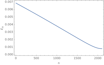
Figure 5: $E_{n}$ represents the difference $x(0)-\Phi(x(0),2\pi)$, in each iteration of Newton’s method.

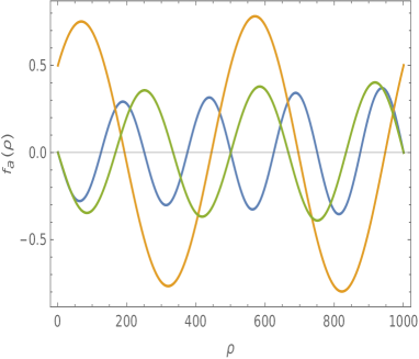
Figure 6: Numerical solution of (101). Left: the different $f_{a}$’s are represented in different colors for a unit of the torus lattice. Right: The compatibility between the three $f_{a}$ solutions is depicted. The red dot in the right figure points out the boundary conditions.

with $x(0)=x_{0}$, $h=\delta\rho$ y $\delta\rho=10^{-2}$ . Due to the way the Newton’s method is designed, it is desirable to start the process with some initial value as close to zero as possible. But, in the absence of any intuition about where the zero might be in this case, we propose a exhaustive search over a coarse grid of the values of $\omega_{i}$ (a "free" parameter) and $f_{a}$ that produce a good approach to the fulfillment of the boundary conditions. From these values, Newton method is applied. The Figure 5 show the difference $x(0)-\Phi(x(0),2\pi)$, in each iteration of Newton’s method.

To summarize this section, we obtain a numerical solution for the non-isotropic Q-ball-like soliton. The shape of the individuals $f_{a}$ are depicted in Figure 6a. Observe that they vary over their period. In figure 6b we can observe the matching of the three different solutions to the system of equations of motion satisfying all of the three constraints with non -vanishing central charge condition.

6 Dynamics of the solutions

In this section we would like to explore the dynamics under a Lorentz Boost and Galilean transformation. Since we are not in a covariant formulation but in a LCG, it is not enough to compute the transformed solutions since it is not guaranteed that the transformed solutions will remain being solutions of the system, hence, we will study them with care.

In first place we will analyze the Lorentz for a generic family of solutions. We define a group velocity ${\bf{v}}=(v_{\sigma},v_{\rho})$ with $v^{2}=|{\bf{v}}|^{2}=v_{\sigma}^{2}+v_{\rho}^{2}$. The worldvolume coordinate transformations imply

$$\sigma\prime =-\gamma v_{\sigma}\tau+\sigma+\left(\frac{v_{\sigma}}{v}\right)^{2}(\gamma-1)\sigma+\frac{v_{\sigma}v_{\rho}}{v^{2}}(\gamma-1)\rho\,,$$ (116)

$$\rho\prime =-\gamma v_{\rho}\tau+\rho+\left(\frac{v_{\rho}}{v}\right)^{2}(\gamma-1)\rho+\frac{v_{\rho}v_{\sigma}}{v^{2}}(\gamma-1)\sigma\,,$$

$$\tau\prime =-\gamma\frac{v_{\sigma}}{c^{2}}\sigma-\gamma\frac{v_{\rho}}{c^{2}}\rho+\gamma\tau\,,$$

with $\gamma=\frac{1}{\sqrt{1-\frac{v^{2}}{c^{2}}}}$ . The function $Z=f(\sigma,\rho)e^{i\omega\tau}$ becomes modified as

$$Z^{\prime}(\sigma\prime,\rho\prime,\tau\prime) =f(k^{\prime}\sigma+l^{\prime}\rho+\omega^{\prime}\tau)e^{i(\alpha\sigma+\Lambda\rho+\eta\tau)}\,,$$ (117)

where

$$k^{\prime} :=k(1+\left(\frac{v_{\sigma}}{v}\right)^{2}(\gamma-1))+l\frac{v_{\rho}v_{\sigma}}{v^{2}}(\gamma-1)\,,$$ (118)

$$l^{\prime} :=l(1+\left(\frac{v_{\rho}}{v}\right)^{2}(\gamma-1))+k\frac{v_{\rho}v_{\sigma}}{v^{2}}(\gamma-1)\,,$$

$$\omega^{\prime} :=-\gamma\left(-kv_{\sigma}+lv_{\rho}\right)\,,$$

$$\alpha :=-\gamma\omega\frac{v_{\sigma}}{c^{2}},\quad\Lambda:=-\gamma\omega\frac{v_{\rho}}{c^{2}},\quad\eta:=\gamma\omega\,.$$

It describes a travelling Q-ball. Clearly the transformed solution acquires a spinning Q-ball ansatz when $f$ does not depend on time, i.e.

$$\omega^{{}^{\prime}}=0=kv_{\sigma}+lv_{\rho},$$ (119)

which imposes a relation between the two components of the group velocity vector.
As we have already explained, a transformed solution is not automatically a solution to the equations of motion. On one side, the functions $f$ must be periodic on the M2-brane worldvolume since $Z$ and $A_{r}$ are single-valued functions. Also, in order to guarantee that the transformed solutions remain in the set of allowed solutions we restrict ourselves to impose them to be in the family of solutions analyzed in section 3. First condition implies that the Fourier modes $(k^{\prime},l^{\prime})$ must be integers and requires the following necessary conditions to be satisfied:

$$\left(\frac{v_{\sigma}}{v}\right)^{2}(\gamma-1)\in Z,\quad\left(\frac{v_{\rho}}{v}\right)^{2}(\gamma-1)\in Z,\quad\quad\frac{v_{\rho}v_{\sigma}}{v^{2}}(\gamma-1)\in Z.$$ (120)

They restrict enormously the possible values of the allowed gamma-factor and group velocities. In order to illustrate it let us consider the following example: assume that $v^{2}/c^{2}=\epsilon^{2}=P/Q$ with $P<Q$ and $v_{\sigma}=1/Nv$, $v_{\rho}=1/Mv$ with $P,Q,N,M\in Z$, this would imply that the following condition is satisfied for example by requiring that $\epsilon^{2}=\frac{n^{2}-1}{n^{2}}$ which leads to $\gamma=n\in Z-\{0\}$ and if $n-1=M^{2}N^{2}$ and then the group velocities becomes $v_{\sigma}=\frac{M}{N}v_{\rho}$ and the necessary conditions are automatically satisfied. Hence, the Lorentz transformed Fourier frequencies are

$$k^{\prime}=k(1+N^{2})+lMN,\quad l^{\prime}=l(1+M^{2})+kMN.$$ (121)

In the example considered, one can see that the allowed $\gamma$ coefficients are discrete and rapidly grows towards the speed of light as $n$ grows. It implies that for this choice of the $v/c$ factor, that the group velocity of the propagating excitations is close to the speed of light, though it does not exclude the existence of other solutions with less group velocity.

These are necessary condition but they do not automatically guarantee the existence of solutions. In the case of the family of solutions verifying (25) and (26) we find that those whose transformed Lorentz $Z$ function must also verify that

$$\alpha=k^{\prime},\quad\Lambda=l^{\prime},\quad\eta=\omega^{\prime}\,,$$ (122)

to remain as solutions of the M2-brane with worldvolume fluxes EOM. See that only $(\alpha,\Lambda)$ impose requirements on

$$(k^{\prime},l^{\prime})=\omega\left(\frac{n+1}{n}\right)(\frac{M^{2}}{v_{\sigma}},\frac{N^{2}}{v_{\rho}}).$$

In the first family case considered in section 3, for the breathing modes $\omega$ given by (45) and $k/l=j$, it is possible to obtain a solution by assuming $\omega=Unv_{\sigma}=Tnv_{\rho}$ with $U,T\in Z$. For example there exists a solution for $M=N=2$, $T=5t$, $U=5\frac{M}{N}t$ with $m_{1}=0,m_{2}\neq n_{2}$ and $m_{2},n_{2},n_{1}>0$ and $\frac{R_{1}^{2}}{R_{2}^{2}}=\left(\frac{m_{2}-jn_{2}}{jn_{2}}\right)\left(\frac{jn_{2}-m_{2}(1-U)}{jn_{1}}\right)>0$ with $t<0$. The transformed Fourier modes become shifted by two different discrete values.

In the case when the $A_{r}$ real scalar field is included, the gauge field also gets transformed. For the ansatz previously previously considered, with $Z(\sigma,\rho)=f(\sigma,\rho)\ e^{i(\lambda(l\rho+k\sigma)+\tau\omega)}$ its Lorentz transformation corresponds to

$$f^{\prime}_{a}(\sigma^{{}^{\prime}},\rho^{{}^{\prime}})=r_{a}\left(\operatorname{cos}[\lambda(l\rho+k\sigma)]+\operatorname{sin}[\lambda(l\rho+k\sigma)]\right)\,,$$ (123)

with the transformed frequency given by

$$\omega^{\prime 2}=\lambda^{2}R_{r}^{2}\left(k^{\prime}m_{r}-l^{\prime}n_{r}\right)^{2}+\lambda^{2}R_{s}^{2}\left(k^{\prime}m_{s}-l^{\prime}n_{s}\right)^{2}=\lambda^{2}\sum_{r}R_{r}^{2}\left(\frac{v_{\sigma}}{c}m_{r}-\frac{v_{\rho}}{c}n_{r}\right)^{2}\,.$$ (124)

See that due to the $A_{r}$ EOM gives a frequency

$$a_{r}\Omega_{r}^{2}=a_{r}\omega^{\prime 2}=\lambda^{\prime 2}\left(a_{r}\left(k^{\prime}m_{s}-l^{\prime}n_{s}\right)^{2}R_{s}^{2}-{a_{s}}\left(k^{\prime}m_{r}-l^{\prime}n_{r}\right)\left(k^{\prime}m_{s}-l^{\prime}n_{s}\right)R_{r}R_{s}\right)\,,$$ (125)

with the amplitude of $A_{r}$ given by

$$a_{r}=\frac{\lambda^{2}}{c^{4}}\left(a_{r}\left(v_{\sigma}m_{s}-v_{\rho}n_{s}\right)^{2}R_{s}^{2}-{a_{s}}\left(v_{\sigma}m_{r}-v_{\rho}n_{r}\right)\left(v_{\sigma}m_{s}-v_{\rho}n_{s}\right)R_{r}R_{s}\right)\,,$$ (126)

and verifying the APD transformed constraint.

$$\sum_{r}a_{r}\left(k^{\prime}m_{r}-l^{\prime}n_{r}\right){R}_{r}=\sum_{r}a_{r}\left(v_{\sigma}m_{r}-v_{\rho}n_{r}\right){R}_{r}=0\,.$$ (127)

The previous equations and the ansatz impose that the frequencies of the Q-ball breathing modes and the temporal dependence of $A_{r}$ become equal, $\omega^{\prime}=\Omega^{\prime}=\Omega_{r}^{\prime}$ with $r=1,2,r\neq s$. Again, it acquires a spinning Q-ball ansatz when a relation between the components of the group vector velocity is imposed,

$$kv_{\sigma}+lv_{\rho}=0,$$ (128)

Let us remind that these solitonic solutions are defined over the M2-brane worldvolume and describe the traveling excitations over the M2-brane with worldvolume fluxes. The center of mass of the M2-brane at this stage propagate as a free particle and its mode is decoupled from the excitations ones mpgm10Monodromy , (as it should happen in case of a particle interpretation). From that point of view, there is not any prerequisite that oblige the excitations to be relativistic, they can behave as classical ones. In principle we consider both approaches to determine the constraints that each of them imposes to the solutions of the theory. In the case of a non-relativistic propagation, the Galileo transformations are obtained for $\gamma=1$, satisfying,

$$\sigma\prime =\sigma-\gamma v_{\sigma}\tau,\quad\rho\prime =\rho-\gamma v_{\rho}\tau,\quad\tau\prime =\tau\,,$$ (129)

implies a modification in the Q-ball expression that acquires a temporal dependence as a traveling wave,

$$Z^{\prime}(\sigma\prime,\rho\prime,\tau\prime)\equiv f(k\sigma+l\rho+\omega^{\prime}\tau)e^{i\omega\tau}\,,$$ (130)

where

$$\omega^{\prime} :=-\left(kv_{\sigma}+lv_{\rho}\right)\,,$$ (131)

In order to keep the solution stationary inside the Q-ball ansatz it is required that $\omega^{\prime}=0$, then the same relation between the group speeds hold

$$kv_{\sigma}+lv_{\rho}=0\,.$$ (132)

See, that this requirement, needs to be fulfilled for every single function $f$ that satisfies the equations. Hence, it holds not only of the analytic family of solutions found in section 3 but for the entire range of solutions analytically or numerically modeled. Indeed, from the numerical point of view, the Galilean transformation can be directly imposed and it does not change the picture of the Q-ball solution already obtained.

7 Topological and nontopological charges of the M2-brane

The supermembrane with worldvolume fluxes contains a topological magnetic monopole associated with the topological constraint central charge and some solutions that also admits a non-topological Q-ball-like in the noncompact variables. It has an associated $U(1)$ Noether charge defined as

$$Q_{a}=\omega_{a}\int d^{2}\sigma f^{2}_{a}(\sigma,\rho).$$ (133)

We can define the Noether charge $Q_{a}$ in terms of its density charge $q_{a}$,

$$Q_{a}=\int d\sigma d\rho q_{a}(\sigma,\rho),\quad\textrm{with}\quad q_{a}(\sigma,\rho)=\omega_{a}f_{a}^{2}(\sigma,\rho)\,.$$ (134)

Then, the Hamiltonian (5), restricted to the Q-ball-like ansatz, with the $A_{r}$ field constant,

$$H=T^{-2/3}\int_{\Sigma}d^{2}\sigma\sqrt{W}\frac{1}{2}[P_{a}^{2}+\frac{T^{2}}{2}(D_{r}f_{a})^{2}]\,.$$ (135)

In order to illustrate it better we will consider the case of the analytic family of solutions satisfying (25). By imposing $\partial_{\rho}f_{a}=j_{a}^{-1}\partial_{\sigma}f_{a}$, then the quadratic contributions become

$$\sum_{r}(D_{r}f_{a})^{2}=\frac{1}{4\omega_{a}q_{a}}\sum_{r}R_{r}^{2}(m_{r}j_{a}^{-1}-n_{r})^{2}(\partial_{\sigma}q_{a})^{2}\,.$$ (136)

When the momentum associated with the $Z$ coordinates is substituted in terms of the Noether charge, then the Hamiltonian can be bounded by below by the following terms

$$H\geq\frac{3}{2}T^{2/3}Q_{a}\omega+\frac{T^{4/3}}{2}\int_{\Sigma}d^{2}\sigma\sqrt{W}\sum_{r}(D_{r}f_{a})^{2}\,.$$ (137)

For the particular case of solutions of the family, the Hamiltonian lower bound expressed in terms of the Noether density charge gets simplified to

$$T^{2/3}H\geq T^{4/3}\frac{3}{2}Q_{a}\omega+\frac{T^{2}}{8\omega_{a}}\sum_{r}R_{r}^{2}(m_{r}-j_{a}^{-1}n_{r})^{2}\int_{\Sigma}d^{2}\sigma\sqrt{W}\frac{(\partial_{\sigma}q_{a})^{2}}{q_{a}}\,.$$ (138)

The mass operator for the M2-brane with fluxes SpinningSolutionsBosonicM2-brane2022 , is bounded by below by the contribution of the topological charges: the central charge (or equivalently $C_{-}$ flux associated with the presence of a monopole), the $C_{+}$ flux contribution and the Kaluza Klein charges. The non-topological ones associated with the presence of Q-ball-like solutions and the interaction terms between both types of solitons contained in the mass term $(D_{r}f_{a})^{2}$

$$\mathcal{M}^{2}\geq Q_{topological}^{2}+T^{4/3}\frac{3}{2}Q_{a}\omega+\frac{T^{2}}{8\omega_{a}}\sum_{r}R_{r}^{2}(m_{r}-j_{a}^{-1}n_{r})^{2}\int_{\Sigma}d^{2}\sigma\sqrt{W}\frac{(\partial_{\sigma}q_{a})^{2}}{q_{a}}\,,$$ (139)

where

$$Q_{topological}^{2}=Q_{fluxes}^{2}+Q_{KK}^{2}=\int_{\Sigma}C_{-}+\int_{\Sigma}C_{+}+\left(\frac{m|q\tilde{\tau}-p|}{R[I_{m}\tilde{\tau}]}\right)^{2}\,,$$ (140)

with

$$\int_{\Sigma}C_{-}=4\pi^{2}R_{1}R_{2}T^{2}n^{2}\,,$$ (141)

the units of flux, corresponding to the value of the central charge (24) as originally shown in mpgm10Monodromy ; mpdm2019:flux . See, that the interaction term contains the Noether charge density of the noncompact sector and the winding numbers required to satisfy the central charge condition that implies the presence of the magnetic monopole. Due to the interaction term, (responsible for the change in the spectral properties), the characteristic relation between the energy and the frequency of the breathing modes in a standard Q-ball, acquires an extra term associated with the non-vanishing mass terms that add a new dependence on the frequency, that leads a relation between the Energy, the Noether charge, the topological winding numbers and the density Noether charge relations. For $T=1$ it is,

$$\frac{\partial E}{\partial\omega}=\frac{3}{2}\sum_{a}Q_{a}+\frac{1}{8\omega_{a}^{2}}\Theta\int_{\Sigma}d^{2}\sigma\sqrt{W}\frac{(\partial_{\sigma}q_{a})^{2}}{q_{a}}\,,$$ (142)

with $\Theta=\sum_{r}R_{r}^{2}(m_{r}-un_{r})^{2}$. In this analysis $f_{a}$ is an arbitrary function of the family. This type of dependence has been also found in the recent paper MappinggaugedQ-balls in which they discuss Q-balls beyond thin-wall limit.

If now we restrict to the analytic family of solutions considered in section 3, we can observe that for $j_{a}=1$ we can integrate the function and obtain the standard dependence for a Q-ball $\frac{\partial E}{\partial\omega}=\frac{3}{2}\sum_{a}Q_{a}$ shifted by a constant term.

8 Discussion and Conclusions

In this paper we provide the first exact solutions of the dynamics of a supermembrane compactified on a target space $M_{9}\times T^{2}$ with a nontrivial $C_{\pm}$ fluxes. We have focused in obtaining Q-ball-like solutions defined on the M2-brane worldvolume. These are solutions to the complex scalar fields $Z_{a}$ that determine the embedding of the supermembrane on the non-compact dimensions. We have analyzed them satisfying the ansatz $Z_{a}=f_{a}(\sigma,\rho)e^{i\omega\tau}$. The name of Q-ball has been maintained, though the solutions characterize solitons over a torus, since the spatial part of the worldvolume of the supermembrane is assumed to be Riemann surface of genus one $\Sigma_{1}$ -it could also have been denoted as Q-torus-. The system is in the presence of a symplectic gauge field defined on the M2-brane worldvolume whose components are defined in terms of derivatives of a single-valued real scalar field $A_{r}$. Both fields $Z_{a}$ and $A_{r}$ define the dynamics of the M2-brane with a system of nine coupled nonlinear equations of motion. The dynamics is restricted by two constraints, the area preserving diffeomorphisms (APD) that is the residual first class constraint of the membrane theory, and the flux condition. This last topological condition implies the so-called central charge condition MARTINRestucciaTorrealba1998:StabilityM2Compactified , which is restriction on the M2-brane wrapping numbers.

We obtain solutions to the dynamics of the M2-brane when the system is isotropic $Z_{a}=Z$ and non-isotropic. In the first case we characterize them analytically and numerically, and numerically in the second one. The analytic solutions are obtained in the presence of a non-vanishing $A_{r}$ field and attending to the type of time dependence imposed on the $A_{r}$ fields, they are organized into two different families. Both cases generate a symplectic gauge field $\mathbb{A}=dA$. In the first case, the temporal dependence on $A_{r}$ is linear. The frequencies characterizing the Q-ball breathing modes are discrete and they are parametrized in terms of the compactified target space moduli, the nontrivial wrapping of the M2-brane, and the amplitudes of the $A_{r}$ field. The Area Preserving Diffeomorphisms (APD) constraint is automatically satisfied. We obtain dynamical solutions to the system that satisfy the central charge restriction and hence the worldvolume flux condition. In the second family, the dependence of $A_{r}$ on $\tau$ is generalized. The associated symplectic field strength depends on all of the variables. Due to the ansatz chosen and the APD constraint a restriction to the EOM appear that leads to a relation between the dispersion relation of the Q-ball breathing modes $\omega$ and the dispersion relation $\Omega$ associated with the $A_{r}$ field. Both frequencies remain discrete. The APD constraint impose a restriction in the amplitudes of the $A_{r}$. For a fixed relation between them, a ratio between the Fourier modes is determined. The type of solutions considered satisfy the central charge condition for winding charges suitably chosen.

We also study their dispersion relations. We obtain that the system presents generically a dispersion, although it also admit solutions with no dispersion for a non-vanishing central charge. Usually solitons are associated with solutions in which the dispersion effects are compensated by the non-linearities of the equation. In our case we find these type of solitonic solutions free of dispersion effects, but also a second type of solitons, that in spite of the dispersion effects, and due to the periodicity of the functions on the M2-brane worldvolume remain being solitons. It can be better understood if we realize that the bosonic potential of the M2-brane contains terms that resemble a quartic harmonic oscillator. Examples of periodic solitons with dispersion effects have been considered in the context of optic solitons Dispersion-Managed:TURITSYN2012 . The dispersion effects in this context do not mean that the system present any lost in energy of the system. Energy is conserved since it corresponds to the excitations on a single M2-brane that propagates freely in the space.

We also investigate the superposition law for the analytic family of solutions found. To this end we find a new method that we denote vectorization, that allows to convert the non-linear differential equations in terms of algebraic expressions, much simpler to solve. We find that, in spite that the EOM associated with the field $A_{r}$ is identically satisfied for a single soliton, due to the nonlinearities of the system of equations, this equation has to be taken into account in the superposition of solutions. We obtain a multi-solitonic solution characterized by a linear superposition, but only when the Fourier modes $k,l$ are equal. This is consistent with the fact that they are solution to the system of nonlinear equations. In the literature it has appeared other optical soliton cases that under restricted conditions admit linear superpositions. See for example, LinearSuperpositionPonomarenko2002 ; ZHOU20171697:LinearSuperpositionPrinciple ; SuperpositionsBrightanddarksolitons .

The previous exact analytic families of solutions are obtained for isotropic coordinates $Z_{a}$ equal for all $a=1,2,3$.

We also have found solutions numerically. From the viewpoint of numerical computation, we have proposed and implemented strategies to find approximate solutions of the Q-ball in the isotropic and non-isotropic cases. In the isotropic case, a fine-difference scheme is used to solve the eigenvalue problem (72), and then the resulting eigenfunctions are used to represent the solution of (73). This transforms the equation (73) into a system of nonlinear algebraic equations, whose solution can be obtained using methods such as Newton’s method. The non-isotropic case for constant $A_{r}$ introduces the non-linearities of the $Z$ equation (not only due to the $A_{r}$ EOM). In this case, the solution of the system (101), is approximated using a shooting method where the gradient of the solution is approximated using finite differences.
In both cases, very simple approximation schemes are used with solutions that present reasonable approximation errors, so we suppose that more sophisticated schemes could produce better solutions even though they have a higher computational cost. Hence, for the isotropic and non-isotropic case, with a vanishing symplectic gauge field, we are able to obtain numerically a Q-ball soliton solutions to the M2-brane with worldvolume fluxes.

The dynamics of the analytic families of solutions is also investigated. We consider Lorentz transformations. Since we work in the LCG, the transformed solutions are not automatically solutions of the EOM. In this sense, we have shown some examples of where we have obtained the necessary restrictions to satisfy the EOM. Since we are considering solutions that represent solitons defined over the worldvolume, -they correspond to excitations on a M2-brane which propagates freely on the space-, it is not necessary that the excitations will be relativistic. We also obtain their Galilean transformations. In this case we find, for the examples considered, that the Galilean transformations restrict further the solutions allowed. We find that for the ansatz considered only those that preserve their Q-ball shape are allowed, i.e. only contain breathing modes but the pulse does not propagate. However, it does not exclude that more general solutions could be obtained by choosing different ansatzs.

The M2-brane mass operator is bounded by below by the topological contribution due to the flux condition and the Kaluza-Klein terms, and for these type of solutions, it is also bounded by below by the Q-ball contribution and a new interaction term between them. The M2-brane with worldvolume fluxes induces a central charge condition that describes a magnetic monopole MARTINRestucciaTorrealba1998:StabilityM2Compactified , and at the same time it may also describe a non-topological Q-ball soliton. We show that there are nontrivial interaction terms between these two, through the mass terms of the potential containing the winding charges that generate the monopole charge and the Noether charge. They describe a relation between the energy $E$ and the frequency $\omega$ that contains on top of the standard term characterizing the Q-ball, a correction to the Q-ball relation that reflects the interaction among those terms. This type of correction, that here has a topological origin, has also appeared in the literature, in a different context, when going beyond the thin-wall limit Heeck_2022:ExcitedQ-balls ; MappinggaugedQ-balls ; Nugaev2020:ReviewNontopologicalSolitons . Recently, it has been discovered a new type of solitons which share these two types of properties. They have been named as monopole-Q-ball soliton and their Q-ball solutions show an increased stability due to the effect of the topological charge. We expect that in our case, the interaction terms will also provide more stability to the Q-ball. The stability properties study are left for a future work.

In summary, we have obtained Q-ball-like solitons solutions of the dynamics of the supermembrane propagating on $M_{9}\times T^{2}$ once that the flux condition is imposed. See, that the non-linearities are present even in the case when the symplectic gauge field vanishes and this is due to the residual equation associated with the presence of multivalued modes that generate the topological magnetic monopole soliton and from those inherited from the quartic potential contribution.

- (1) S. Coleman, Q-balls, Nucl. Phys. B 262 (1985) 263 .
- (2) V. Loiko and Y. Shnir, Q-balls in the u(1) gauged friedberg-lee-sirlin model, Phys. Lett. B 797 (2019) 134810.
- (3) J. Heeck, A. Rajaraman, R. Riley and C.B. Verhaaren, Mapping gauged -balls, Phys. Rev. D 103 (2021) 116004.
- (4) A.Y. Loginov, Nontopological soliton configuration in system involving three interacting scalar fields and obeying global u(1) × u(1) symmetry, también lo aplica en q-balls, Physics of Atomic Nuclei 70 (2007) 945.
- (5) A. Alonso-Izquierdo, D. Miguélez-Caballero, L. Nieto and J. Queiroga-Nunes, Wobbling kinks in a two-component scalar field theory: Interaction between shape modes, Physica D: Nonlinear Phenomena 443 (2023) 133590.
- (6) M. Axenides, S. Komineas, L. Perivolaropoulos and M. Floratos, Dynamics of nontopological solitons: Q balls, Phys. Rev. D 61 (2000) 085006.
- (7) E. Palti, P.M. Saffin and E.J. Copeland, Dynamics of q-balls in an expanding universe, Phys. Rev. D 70 (2004) 083520.
- (8) I.E. Gulamov, E.Y. Nugaev, A.G. Panin and M.N. Smolyakov, Some properties of -balls u(1) gauged q-balls, Physical Review D 92 (2015) .
- (9) M. Tsumagari, The Physics of Q-balls. PhD Thesis, Ph.D. thesis, University of Nottingham, 2009. arXiv:0910.3845. https://doi.org/10.48550/arXiv.0910.3845.
- (10) Y. Bai, S. Lu and N. Orlofsky, Q-monopole-ball: a topological and nontopological soliton, Journal of High Energy Physics 2022 (2022) 109.
- (11) A. Alonso-Izquierdo, A. Balseyro Sebastian, M. Gonzalez Leon and J. Mateos Guilarte, Kinks in massive non-linear s1×s1-sigma models, Physica D: Nonlinear Phenomena 440 (2022) 133444.
- (12) S. Bolognesi and M. Shifman, torus in supersymmetric qed, Phys. Rev. D 76 (2007) 125024.
- (13) A. Kusenko and M.E. Shaposhnikov, Supersymmetric Q balls as dark matter, Phys. Lett. B418 (1998) 46 [hep-ph/9709492].
- (14) S. Krippendorf, F. Muia and F. Quevedo, Moduli stars, JHEP 2018 (2018) 70.
- (15) J. Hoppe and H. Nicolai, Relativistic minimal surfaces, Phys. Lett. B 196 (1987) 451 .
- (16) J. Hoppe, Some classical solutions of membrane matrix model equations, NATO ASI Ser. C Sci. 520 (1999) 423 [hep-th/9702169].
- (17) A. Restuccia and R. Torrealba, Membrane solitons as solitary waves of nonlinear string dynamics, Class. Quantum Grav. 15 (1998) 563 [hep-th/9706111].
- (18) S.-J. Rey, Gravitating M (atrix) Q-balls, arXiv preprint (1997) [hep-th/9711081].
- (19) E. Floratos, G. Leontaris, A. Polychronakos and R. Tzani, Instanton solutions of the self-dual membrane in various dimensions, Phys. Lett. B 421 (1998) 125 .
- (20) E. Bergshoeff and P.K. Townsend, Solitons on the supermembrane, JHEP 1999 (1999) 021.
- (21) R. Portugues, Membrane solitons in eight-dimensional hyper-kaehler backgrounds, JHEP 2004 (2004) 051.
- (22) M. Garcia del Moral, C. Las Heras, P. Leon, J. Pena and A. Restuccia, M2-branes on a constant flux background, Phys. Lett. B 797 (2019) 134924 [1811.11231].
- (23) M. Garcia del Moral, C. Las Heras, P. Leon, J. Pena and A. Restuccia, Fluxes, twisted tori, monodromy and supermembranes, JHEP 09 (2020) 097 [2005.06397].
- (24) I. Martín, A. Restuccia and R. Torrealba, On the stability of compactified d = 11 supermembranes: Global aspects of the bosonic sector, Nucl. Phys. B 521 (1998) 117.
- (25) I. Martin, J. Ovalle and A. Restuccia, Compactified D = 11 supermembranes and symplectic noncommutative gauge theories, Phys. Rev. D 64 (2001) 046001 [hep-th/0101236].
- (26) I. Martin, J. Ovalle and A. Restuccia, D-branes, Symplectomorphisms and Noncommutative Gauge Theories, Nucl. Phys. Proc. Suppl. 102 (2001) 169 [hep-th/0005095].
- (27) M.P. García del Moral, J.M. Peña and A. Restuccia, Supermembrane origin of type II gauged supergravities in 9D, JHEP 2012 (2012) 63 [1203.2767].
- (28) J. Bellorin and A. Restuccia, Minimal immersions and the spectrum of supermembranes, hep-th/0312265.
- (29) J. Hoppe, Quantum theory of a massless relativistic surface and a two-dimensional bound state problem, Ph.D. thesis, MIT, Dept. of Physics, (1982). [1721.1/15717].
- (30) P.T. Allen, L. Andersson and A. Restuccia, Local well-posedness for membranes in the light cone gauge, Commun. Math. Phys. 301 (2010) 383–410 [0910.1488].
- (31) J. Brugues, J. Rojo and J.G. Russo, Nonperturbative states in type II superstring theory from classical spinning membranes, Nucl. Phys. B 710 (2005) 117.
- (32) G.K. Vallis, Atmospheric and Oceanic Fluid Dynamics: Fundamentals and Large-Scale Circulation, Cambridge University Press, 2nd ed. (2017).
- (33) M.A. Agüero Granados and V.N. Serkin, Introducción a la teoría de solitones, Ediciones y Gráficos Eón, SA de CV (2020).
- (34) O. Rosas-Ortiz and S. Cruz y Cruz, Superpositions of bright and dark solitons supporting the creation of balanced gain-and-loss optical potentials, Mathematical Methods in the Applied Sciences 45 (2022) 3381.
- (35) S.A. Ponomarenko, Linear superposition principle for partially coherent solitons, Phys. Rev. E 65 (2002) 055601.
- (36) Y. Zhou and W.-X. Ma, Applications of linear superposition principle to resonant solitons and complexitons, Computers and Mathematics with Applications 73 (2017) 1697.
- (37) R. Haberman, Elementary Applied Partial Differential Equations with Fourier Series and Boundary Value Problem, Prentice Hall (1984).
- (38) P.D. Alvarez, P. Garcia, M.P. Garcia del Moral, J.M. Peña and R. Prado, Spinning solutions for the bosonic m2-brane with c± fluxes, Journal of High Energy Physics 2022 (2022) 28.
- (39) P.-F. Han and Y. Zhang, Linear superposition formula of solutions for the extended (3+1)-dimensional shallow water wave equation, Nonlinear Dynamics 109 (2022) 1019.
- (40) T. Aprille and T. Trick, Steady-state analysis of nonlinear circuits with periodic inputs, Proceedings of the IEEE 60 (1972) 108.
- (41) S.K. Turitsyn, B.G. Bale and M.P. Fedoruk, Dispersion-managed solitons in fibre systems and lasers, Physics Reports 521 (2012) 135.
- (42) Y. Almumin, J. Heeck, A. Rajaraman and C.B. Verhaaren, Excited q-balls, The European Physical Journal C 82 (2022) .
- (43) E.Y. Nugaev and A.V. Shkerin, Review of nontopological solitons in theories with u(1)-symmetry, Journal of Experimental and Theoretical Physics 130 (2020) 301.