Asymptotic confidence sets for random linear programs
Abstract
Motivated by the statistical analysis of the discrete optimal transport problem, we prove distributional limits for the solutions of linear programs with random constraints. Such limits were first obtained by Klatt, Munk, & Zemel (2022), but their expressions for the limits involve a computationally intractable decomposition of into a possibly exponential number of convex cones. We give a new expression for the limit in terms of auxiliary linear programs, which can be solved in polynomial time. We also leverage tools from random convex geometry to give distributional limits for the entire set of random optimal solutions, when the optimum is not unique. Finally, we describe a simple, data-driven method to construct asymptotically valid confidence sets in polynomial time.
Keywords— Linear programming, distributional inference, confidence sets
1 Introduction
Linear programming is one of the core techniques in convex optimization, capturing many canonical problems such as maximum flow, shortest path, bipartite matching, and optimal transport. Linear programs (LPs) are notable for their versatility, their rich combinatorial theory, and their algorithmic tractability: the pioneering work of Hačijan (1979) showed that LPs can be solved in polynomial time, and the last 70 years of research in theoretical computer science and scientific computing have made solving linear programs a “mature technology” in practice (Boyd and Vandenberghe, 2004).
We consider throughout a standard form LP, given by
| (1) |
where , and . The goal of this paper is to understand the distributional behavior of solutions to Eq. 1 when is replaced by a random vector . We assume the existence of a random variable such that
| (2) |
for some rate , and we will seek a corresponding limit law for the solutions to Eq. 1. This setting is motivated by applications of linear programming in statistics and machine learning, where the “right-hand side” vector corresponds to random capacities, demands, or prices. An important example, which motivates many of the developments of this paper, is the linear programming formulation of the optimal transportation problem between discrete distributions, where the vector corresponds to the probability mass function of the two measures. The statistician who only has access to these measures via samples can compute a solution to an empirical optimal transport problem by replacing with an estimator . Quantifying the uncertainty in the resulting solution requires constructing an asymptotic confidence set for this random linear program.
Obtaining distributional limit results for solutions to random optimization problems is, of course, a well studied subject both in scientific computing and in statistics (Shapiro, 1991, Linderoth et al., 2006, Polyak and Juditsky, 1992, Dupačová and Wets, 1988, King and Rockafellar, 1993), but the LP lacks the regularity conditions necessary to apply classical results: neither smoothness nor strong convexity holds for Eq. 1 in general, solutions are generally not unique, and optimal solutions to Eq. 1 always lie on the boundary of the feasible set. By contrast, standard distributional limit results, for instance in the analysis of M-estimators, require local strong convexity, uniqueness, and that the solution to the population-level problem lies in the relative interior of the feasible set (see, e.g., Vaart, 1998). The challenges met in circumventing these classical conditions are well known (Andrews, 2002, Chernoff, 1954, Aitchison and Silvey, 1958). Statistically, the lack of regularity in Eq. 1 is the source of several pathologies: even when the solution to Eq. 1 is unique, the limiting distribution will in general not be Gaussian, and if there are multiple solutions to Eq. 1 it is not even clear how to formulate the desired distributional limit results. The typical path forward, not taken in this work, is to impose extra conditions to guarantee that uniqueness holds and to focus on settings where there is sufficient regularity to ensure a Gaussian limit.
Let us give a very simple example which illustrates some of the difficulties of this problem. Consider a optimal transport problem:
where . In this case, the target solution is unique. If we suppose that is replaced by random vector in the probability simplex , then the optimal solution to the perturbed program is
and if we assume converges in distribution to a centered Gaussian vector, the rescaled solution converges to a mixture distribution with two non-Gaussian components. A version of the same problem, with the same objective function and , has multiple optimal solutions, and a priori it is not clear how to quantify the uncertainty of a solution obtained when is replaced by a random counterpart.
The challenges in obtaining distributional limits for LPs were first tackled by the pioneering work of Klatt et al. (2022), who derived distributional limits for (1) in a very general setting. Their results are expressed in terms of a partition of into closed convex cones; the restriction of the limiting distribution on each cone is a linear function of the limit of the sequence . To handle the fact that solutions to (1) may not be unique, Klatt et al. (2022) adopt a framework of an algorithmic flavor: they assume, informally speaking, that there exists a consistent, possibly randomized, selection procedure to specify a solution within the optimal set. This strategy allows them to prove a distributional limit for the particular optimal solution selected by this procedure, without having to assume that the optimal solution is unique.
Despite the completeness and sophistication of their approach, Klatt et al. (2022) leave open several fundamental questions. First, it is not clear whether it is possible to sample from their limit laws in polynomial time: all of their limits are expressed in terms of a decomposition of into a possibly exponential number of closed convex cones. Even evaluating the functions involved in their limiting expressions therefore appears to be computationally intractable. Second, their approach to non-unique solutions cleverly sidesteps the need to assume that the optimal solution is unique; however, the resulting limit law does not give insight into the overall geometry of the random solution set. Third, even ignoring issues of computational feasibility, their results do not yield a method to obtain asymptotically valid confidence sets from data, because the limiting distributions they obtain depend on the (typically unknown) optimal solutions to the original LP.
In this work, we propose solutions to these three questions. First, in the case the solution to the original LP is unique, we give a new representation of the limit that can be sampled from in polynomial time; in fact, we show that the limit can be generated by solving an auxiliary random linear program. Second, in the general (non-unique) case, we define and prove a distributional limit for the optimal solutions in the space of convex sets—the resulting limit captures the random geometry of the entire solution set. Finally, we develop a practical and computationally cheap data-driven method for constructing asymptotically valid confidence sets.
2 Preliminaries on linear programming
In this section, we recall some facts about the structure of linear programs. We point the reader to standard reference works (Nocedal and Wright, 2006, Bradley et al., 1977, Boyd and Vandenberghe, 2004, Bertsimas and Tsitsiklis, 1997) for additional background information.
We denote the set of optimal solutions to (1) by
| (3) |
The notation emphasizes that this optimal set depends on the right-hand side . In general, LPs do not possess unique solutions, so that typically . However, if the solution is unique, by slight abuse of notation we write for both the (single-element) set of optimal solutions and for the optimal solution itself. We sometimes refer to as the set of “target solutions,” to contrast it with the random soultion set obtained by replacing by its random counterpart. We denote the optimal objective value of (1) by .
Throughout, we make the following assumptions on (1).
Assumption 1.
The assumption that is full rank is without loss of generality, as redundant constraints in the matrix can always be removed. The assumption that is nonempty and bounded is also made by Klatt et al. (2022) and holds for many LPs of interest, including optimal transport problems. Finally, the Slater condition is a standard assumption in convex programming and is only a minor strengthening of Assumption (B2) of Klatt et al. (2022, see Lemma 5.4).
2.1 Bases
For any subset , we denote by the submatrix of formed by taking the columns of corresponding to the elements of . Analogously, for , we write for the vector of length consisting of the coordinates of corresponding to .
Definition 1.
A set is a basis if
| (4) |
Given a basis , we can define the basic solution to be the vector satisfying
| (5) | ||||
Explicitly, is defined by setting the coordinates not in to zero and inverting the matrix to obtain the values on the coordinates corresponding to . This vector is a feasible solution to (1) if and only if the vector is nonegative; if it is, we say that is a basic feasible solution. By construction, basic feasible solutions have at most non-zero entries: if we denote the support (i.e., the set of non-zero entries) of a vector by , then
This inclusion can be strict if the vector has zero coordinates. When the inclusion is strict, the solution is called degenerate. If is a degenerate basic feasible solution, then any basis such that satisfies ; in particular, several different bases may give rise to the same (degenerate) basic feasible solution.
Geometrically, basic feasible solutions are precisely extreme points (vertices) of the feasible set of (1) (Bertsimas and Tsitsiklis, 1997, Theorem 2.3); we will therefore use the terms basic feasible solution and vertex interchangeably in what follows. Our justification for focusing on basic feasible solutions is the “fundamental theorem of linear programming” (Bertsimas and Tsitsiklis, 1997, Theorem 2.7), which ensures that if any optimal solution to (1) exists, then there exists an optimum which is a basic feasible solution.
We denote by the set of all bases for which is a basic feasible solution, and by the set of all bases for which is an optimal solution. The set of optimal vertices of (1) is defined by
| (6) |
The general theory of polyhedral geometry implies that since is bounded, we may write , the convex hull of . Moreover, the assumption that is bounded implies that is bounded for all perturbations .111This follows from the fact that and are polyhedra with the same recession cone, which must equal since is bounded. We therefore also have .
| Symbol | Meaning |
|---|---|
| Optimal objective value of (1) | |
| , | True and random right-hand side constraints, (2) |
| Set of nonzero coordinates of | |
| Set of optimal solutions, (3) | |
| Basic feasible solution, (5) | |
| , | Set of feasible and optimal bases |
| Extreme points of , (6) | |
| Support function of , (9) |
We summarize the main notation used in this paper in Table 1.
3 Vertex and base stability
This section presents two stability results that are central to our analysis. Though simple and likely well known, we present them explicitly here to highlight the important role they play in our theorems.
The first is a Lipschitzian property of polytopes due to Walkup and Wets (1969), which shows that the set of optimal solutions of Eq. 1 is Lipschitz with respect to the Hausdorff distance.
Proposition 1.
Under 1, there exists a constant such that if are such that and are nonempty, then .
The second proposition shows that optimal bases for are also optimal for .
Proposition 2.
Under 1, there exists such that if , then is nonempty and .
4 A tractable limiting distribution when the target solution is unique
In this section, we first consider the simplified setting where the target solution is unique. Even under this simplification, however, the limiting distribution obtained by Klatt et al. (2022) does not have a tractable form. In particular, it is not even clear whether it is possible to generate samples from this distribution in polynomial time. The goal of this section is to obtain an expression for the limiting distribution that can be computed efficiently.
Stating this result requires defining a notion of distributional convergence suitable for a random set. Even when , it is possible that . This situation can arise when is unique but degenerate, i.e., when there exist multiple optimal bases in . Even if these bases all give rise to the same solution in the original program, they can correspond to different optimal solutions when is replaced by . In this situation, , and it is not possible to formulate a distributional limit for viewed as the difference of two vectors in . However, when , we can consider the set defined by translating the elements of by and rescaling them by :
Our first main result is that this random set enjoys a set-valued distributional limit, with limit equal to the distribution of the optimal set of a random auxiliary linear program.222To define weak convergence in this setting, we view these random sets as random elements in the metric space of compact subsets of equipped with the Hausdorff distance, and weak convergence means, as usual, the convergence of expectations of bounded, continuous functions in this topology (Molchanov, 2005, King, 1989).
Theorem 3.
The continuous mapping theorem implies that continuous functionals of the set also enjoy weak convergence. To give a concrete example of the statistical implications of this fact, consider the problem of obtaining a confidence set for . Doing so requires knowing how far typically is from . If we let , then the following corollary shows that we can obtain a distributional limit for .
Corollary 4.
.
In words, the rescaled distance of the target solution to the set of optimal solutions of the random program converges in distribution to the distance of zero to the optimal set of the random auxiliary LP. Importantly, this is a convex program, whose solution can be found in polynomial time.
Let us compare Corollary 4 with what would be obtained by a more standard approach. If one finds estimators by solving an optimization problem that can yield multiple optima, a standard path to inference consists in first identifying a subset of them that are close to one another, and then deriving the limiting distribution of any one of them, relative to the unique target. By contrast, Corollary 4 gives information about the distance of to the whole set of optima for the random program.
We stress our limit law is equivalent to the one obtained by Klatt et al. (2022, Theorem 3.5). The benefit of Theorem 3 is that is given explicitly: though this set can be large, it is algorithmically accessible since it possesses an explicit polyhedral representation in terms of separating hyperplanes. This implies, for instance, that it is possible to solve convex optimization problems involving in polynomial time via the ellipsoid method . On the other hand, Klatt et al. (2022) prove the same result but where the expression on the right side is a sum over a decomposition of into a possibly exponential number of pieces; such a decomposition typically cannot be evaluated in polynomial time.
When the unique optimal solution is also non-degenerate, then Proposition 2 implies that for sufficiently close to , the perturbed linear program also possesses a unique solution. In this situation, Theorem 3 is a standard distributional limit: asymptotically almost surely, the set reduces to a singleton, and Theorem 3 shows that the distributional limit of the vector is the (unique) solution to Eq. 8, which is just for the unique . This recovers the limit for this simplified setting mentioned by Klatt et al. (2022, discussion after Remark 3.2).
5 Distributional convergence in the space of convex sets
When is not unique, the approach to defining a set-valued distributional limit taken in Theorem 3 no longer succeeds. Indeed, if and are general closed sets, then even if in Hausdorff distance, the set
will not converge to in general, so that no meaningful limit of exists. In the non-unique case, Klatt et al. (2022) therefore define a distributional limit under the additional assumption that there exists a consistent scheme for selecting a single element of and ; they then show that this selection satisfies a distributional limit in the classical sense. This ingenious approach captures the behavior of practical algorithms for solving LPs, since reasonable LP solvers give rise to such selection schemes (see Klatt et al., 2022, Lemma 5.5). However, as in the case where the target solution is unique, their limiting distribution is expressed as a sum over a decomposition of into a possibly exponential number of pieces. Moreover, their techniques do not give insight into the overall fluctuations of the random set . By contrast, in the unique case, Theorem 3 shows that it is possible to obtain simultaneous control over the whole random set.
In this section, we leverage techniques from random convex geometry to obtain similar results for the non-unique case. Unlike Theorem 3, Theorem 5 goes beyond the setting analyzed by Klatt et al. (2022). Like Theorem 3, we state our convergence results in terms of the optimal solutions to a random auxiliary LP, implying that evaluating the limits we obtain can be computationally tractable in applications.
To formulate our distributional limit, we adopt a strategy developed by Artstein and Vitale (1975), Weil (1982), and independently by Lyashenko (1983) to prove central limit theorems for random compact sets. To any compact, convex set , we associate its support function defined by
| (9) |
The mapping provides an isometric embedding of the metric space of convex, compact sets equipped with the Hausdorff metric into the Banach space of continuous functions on the sphere equipped with the uniform norm (see Molchanov, 2005, section 3.1.2). Explicitly, given two compact, convex sets and , we have
| (10) |
In particular, the map from a convex set to its support function is injective; can be recovered from by taking its Legendre transform. This embedding has two profound implications. First, the geometry of convex sets is entirely captured by their support functions. In particular, we may associate to a random convex set its support function, viewed as a random element of , and study its distribution instead.333We omit a detailed discussion of measurability here, but it can be shown that if the space of convex, compact subsets of is equipped with an appropriate -algebra (known as the Effros -algebra), then for a random set the support function is indeed a random variable in (see Molchanov, 2005, Proposition 2.5). Second, since is a Banach space, we may leverage the theory of probability in Banach spaces to prove limit theorems for support functions.
Our main result of this section is a distributional limit for the set . Once again, it is stated in terms of the solutions to an auxiliary linear program.
Theorem 5.
Let and be the support functions of and , respectively. Suppose that (1) satisfies 1. If satisfies the distributional limit (2), then
| (11) |
where is the random element of defined by
and is the set of optimal vertex solutions to the following linear program:444The function is only differentiable almost everywhere, but since is almost surely continuous it suffices to specify its values on a dense subset.
| (12) |
Informally, Theorem 5 shows that when is large, . By the isometry described in Eq. 10, this translates into a statement about the fluctuations of the random set around . The proof of Theorem 5 is based on establishing the directional Hadamard differentiability of the mapping viewed as a function from to , and then applying a functional delta method due to Römisch (2006).
Like Theorem 3, Theorem 5 has statistical implications for the problem of obtaining a confidence set for . The isometry (10) implies the following analogue of Corollary 4.
Corollary 6.
In other words, the rescaled Hausdorff distance between the solution sets converges in distribution to the supremum of a random continuous function on the sphere. Corollary 6 can be compared to (Klatt et al., 2022, Proposition 3.7), which shows that . Our result gives finer control over the behavior of the rescaled distance in terms of the solutions to auxiliary linear programs. However, unlike Corollary 4, we are not aware of an algorithm that can compute the supremum on the right side of Corollary 6 in polynomial time. Finding a computationally tractable expression for this limit is an attractive open problem.
6 Data-driven confidence sets
Theorems 3 and 5 give explicit distributional limits for in terms of auxiliary linear programs. Though evaluating these limits is computationally tractable, they fail to be suitable for concrete inference tasks because the limiting distributions depend on properties of the true optimal solution set . Since this set is almost always unknown in practice, Theorems 3 and 5 do not provide a data-driven way to obtain asymptotically valid confidence sets.
In principle, the fact that Theorem 5 is proven by directional Hadamard differentiability arguments implies that the -out-of- bootstrap is consistent (Dümbgen, 1993). However, using the bootstrap for inference raises other practical difficulties: it is an open question how to choose for good performance, and convergence is slow. Therefore, even though Theorems 3 and 5 provide a complete answer to the theoretical question of obtaining a valid distributional limit, they are a poor way to construct confidence sets in practice.
In this section, we give a simple procedure to obtain such sets. Specifically, we suppose that that statistician has solved the perturbed linear program and obtained a random solution along with a corresponding basis .555Algorithms such as the simplex method always return an optimal vertex when one exists, along with a corresponding basis (Bertsimas and Tsitsiklis, 1997, Theorem 3.3). We will construct a confidence set based on that is guaranteed to contain at least one element of with high probability. Specifically, let us consider the basic solution defined by the random basis . This solution may not be feasible for (1), much less optimal, so we define the projection
| (13) |
The following result shows that we can construct a set containing this point with high probability.
Theorem 7.
Corollary 8 (Confidence set for an optimal solution).
In the setting of Theorem 7, the set contains an element of with asymptotic probability at least .
Theorem 7 and Corollary 8 are weaker than Theorems 5 and 3: they do not give any information about the whole set of optimal solutions . Instead, Corollary 8 only guarantees that contains an optimal solution with high probability. As our simulations in Section 7 show, when the optimal solution is non-unique, the confidence sets constructed by this procedure sometimes cover one solution, sometimes another. Nevertheless, Corollary 8 does offer the practitioner an asymptotic guarantee that some optimal solution is in a neighborhood of the estimator.
On the other hand, unlike Theorems 5 and 3, Corollary 8 is eminently practical. It requires only the outputs and from a standard linear programming algorithm, and the set is easy to compute, since the mapping is an explicit linear transformation. For instance, if is an ellipsoid of the form , then recalling definition (5) in Section 2 we have
| (15) |
where .
7 Examples
We will provide two examples in this section to show the effectiveness of the method described in Theorem 7 and Corollary 8 for generating a confidence set for solutions to LPs.
We first return to the simple discrete optimal transport problem described in the introduction, which is a linear program with a unique degenerate optimal vertex. We then treat a more complicated example arising from a min-cost flow problem (see Bradley et al., 1977, section 8.1). In this example, there are two optimal vertex solutions at the population level. In both cases, our simulations confirm that the method gives confidence sets which cover an optimal solution with high probability.
7.1 Empirical Optimal Transport
We consider the optimal transport example given in the introduction, where we suppose that . This corresponds to the situation where we aim to estimate the solution to an optimal transport problem involving an unknown distribution on the basis of i.i.d. samples from . In this setting, the classical central limit theorem implies , where . We therefore choose , where is a 95% confidence interval for an random variable, and use Corollary 8 to construct a confidence set for the entries of .
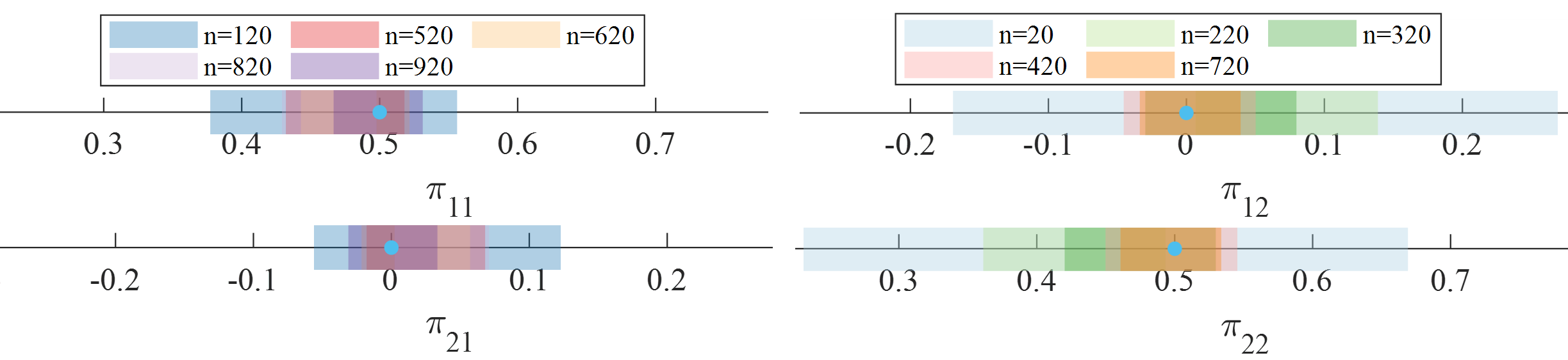
Figure 1 shows examples of the confidence intervals produced by our method. We plot one realization for each of the labeled values of . Note that for each realization, the confidence intervals for two (random) entries of are singletons: for example, when , the solution we obtained to the LP was and the confidence intervals given by Corollary 8 were , , and . Even though the confidence intervals for and have zero width, this set does in fact contain the optimal solution . The somewhat counterintuitive fact that a confidence set with empty interior covers the true parameter with probability approaching is a consequence of the fact that the distribution of is not absolutely continuous with respect to the Lebesgue measure.
We also estimate the observed coverage probabilities for finite . For each , we generate independent replicates, calculate the confidence intervals and count the replicates that successfully capture a true solution.
| n | ||||||||
|---|---|---|---|---|---|---|---|---|
| Coverage Probability |
7.2 Minimal Cost Flow Problem
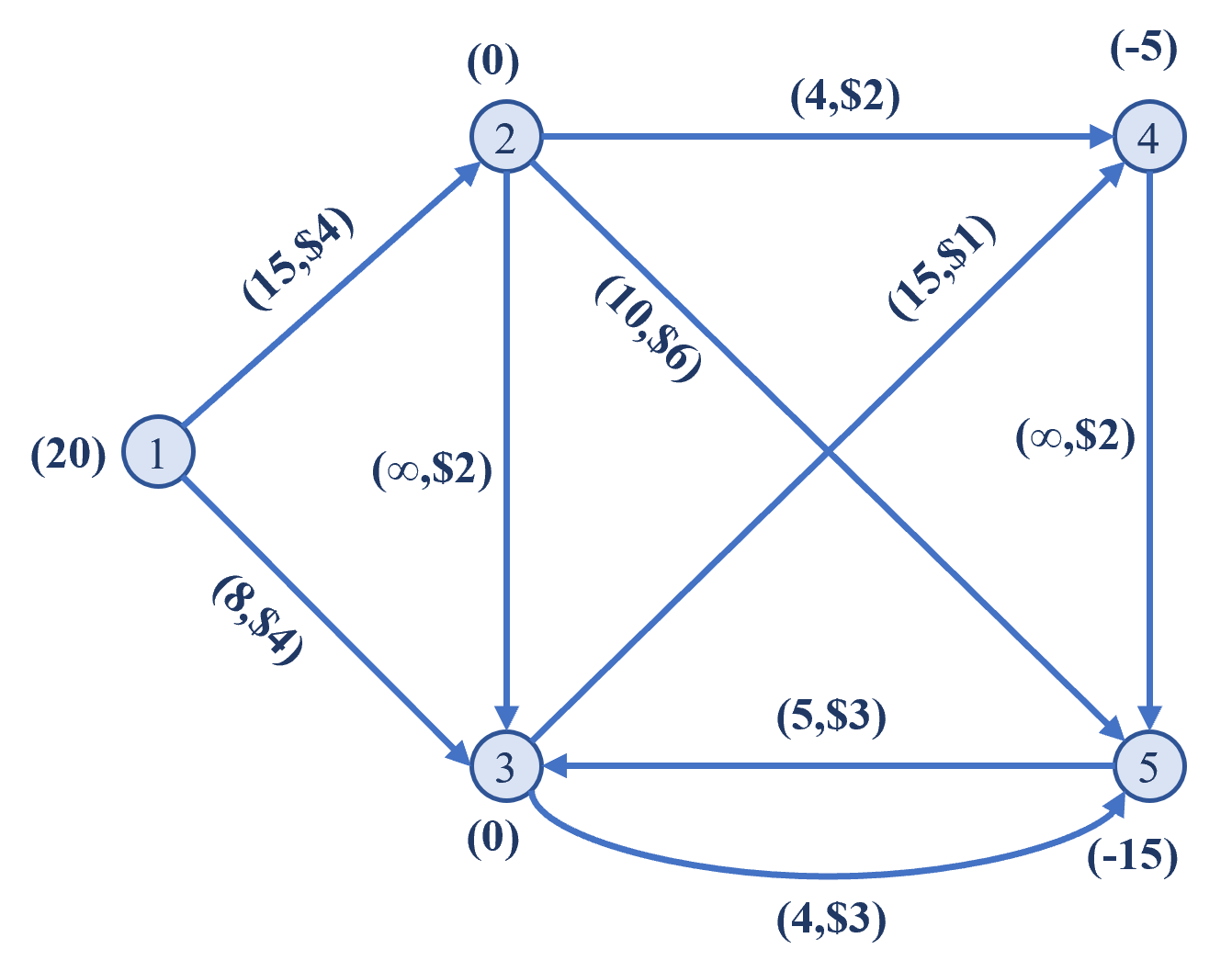
We adapt an example from Bradley et al. (1977, Section 8.1) arising in operations research. Consider the problem of moving goods from origins to destinations along routes with certain volume constraints and costs. We model an instance of this problem as the directed graph depicted in Fig. 2, with nodes and arcs. Each arc is unidirectional, labeled with its capacity and transportation cost (the pair of numbers in the parentheses adjacent to the arc). Each node is labeled with its supply or demand. For example, the supply of node is . The arc transports products from node to node with the maximum capacity of units of product and the cost per unit of product. Assuming that the total demand matches the total supply, the goal is to fulfill all the demands in the network at a minimum cost.
This minimal-cost flow problem can be written in a linear program form:
| (16) |
where is the supply of each node, is the capacity of each arc, and is the transportation cost of each arc. A standard linear program in the form of Eq. 1 can be obtained for this problem by introducing the auxiliary variable , which satisfies and . The auxiliary variable represents the remaining capacity for each arc. The standard form for Eq. 16 is
| (17) |
Note that the equality constraints are redundant due to the flow balance condition of the network, and deleting any one of them will not change the program. Suppose the flow balance constraint on the third node is deleted and we have the modified supply vector .
The program in Fig. 2 has two optimal vertex solutions:
| solution 1 | 12 | 8 | 8 | 4 | 0 | 15 | 1 | 14 | 0 |
|---|---|---|---|---|---|---|---|---|---|
| solution 2 | 12 | 8 | 8 | 4 | 0 | 12 | 4 | 11 | 0 |
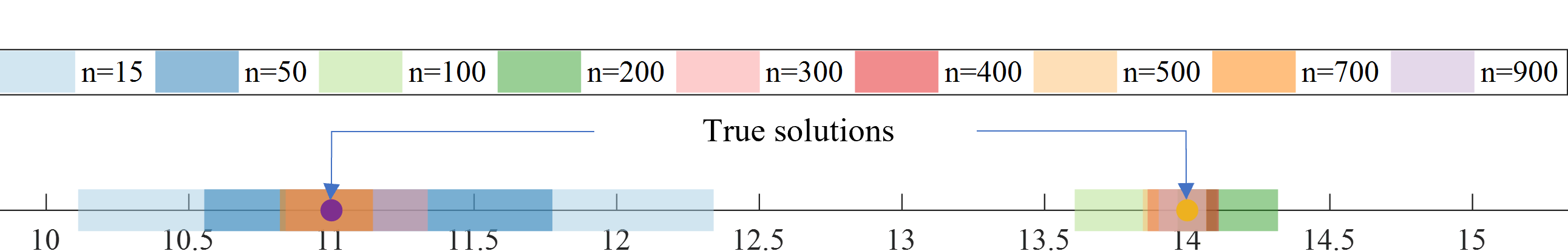
In applications, the true supply and demand at each node may not be known precisely, but rather must be estimated by an empirical supply vector obtained by averaging the observed supplies and demands over days. Suppose that we know , where . We calculate a min-cost flow using the estimated supply vector , and employ Corollary 8 to build a confidence set.
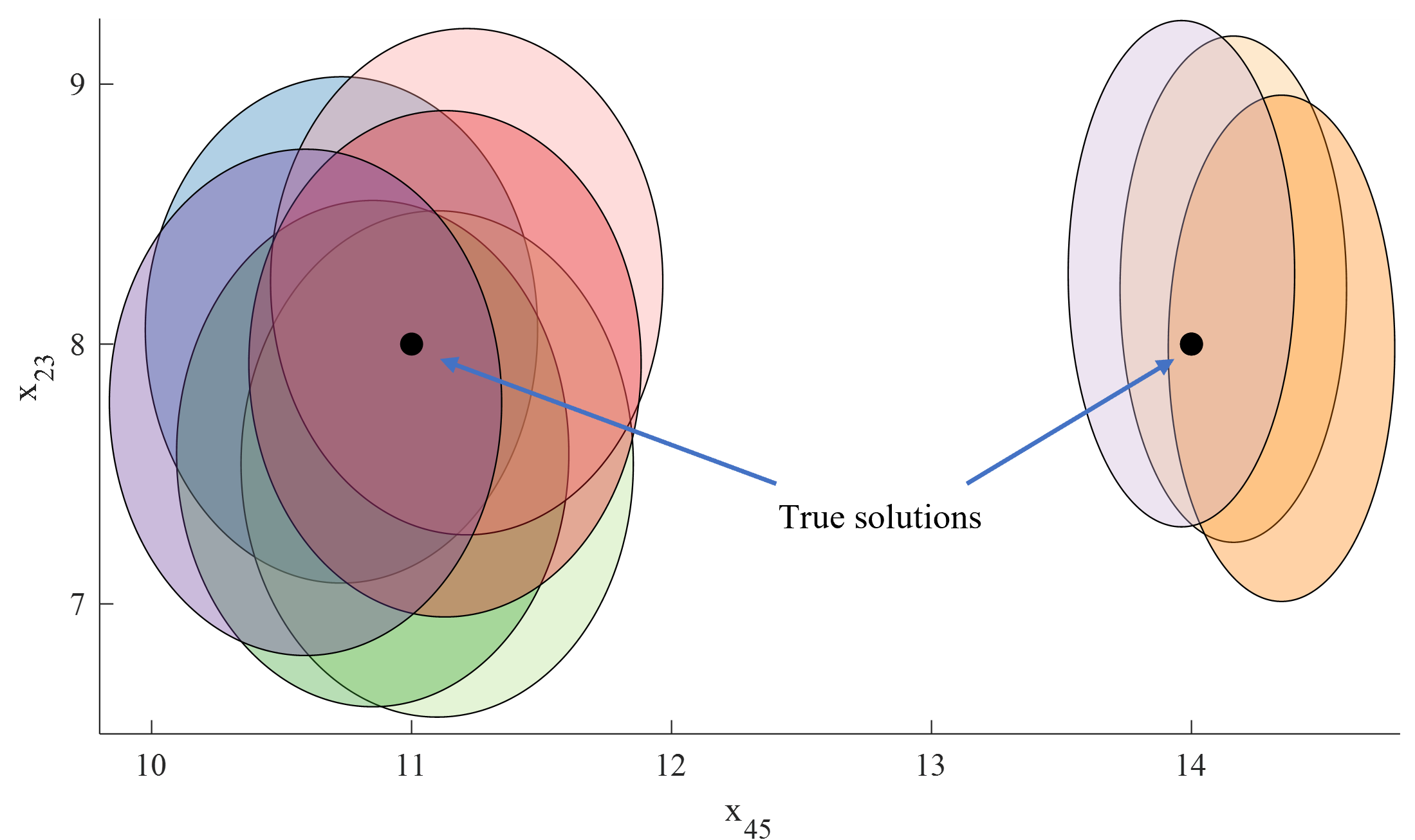
To visualize the confidence set for for various , we show the projection of dimensional confidence sets to lower dimensional spaces. As an example, we plot the confidence interval for the coordinate (Fig. 3, Fig. 4) and the confidence set for the dimensional arc pair (Fig. 5). In Fig. 3, we show several examples of the confidence sets we obtain for . We plot a single realization for each value of . Figure 4 shows many replicates for the case to illustrate the sampling variability of the sets we construct, and Fig. 5 depicts the same procedure for the two-dimensional confidence set for . We can see that for each replicate, the given confidence sets capture one of the solutions very well—which solution is covered depends on the random fluctuations in each replicate.
In short, Corollary 8 gives a practical means of obtaining asymptotically valid confidence sets for the solution to a linear program. To our knowledge, this is the first procedure satisfying these requirements.
Acknowledgements
Bunea was supported in part by NSF grant DMS-2210563, and Niles-Weed was supported in part by NSF grant DMS-2210583 and a Sloan Research Fellowship.

Appendix A Proofs of propositions
We first establish a few basic lemmas. In the proofs, we utilize the optimal conditions of the linear program Eq. 1 and its dual program:
| (18) |
The linear program Eq. 1 and the dual program Eq. 18 achieve their optima at if and only if such that:
| (19) |
The last condition is called complementary slackness, and is equivalent to the condition that for all .
Lemma 9.
Under 1, there exists , , and such that the following properties hold:
-
1.
If , then
-
2.
If , then
-
3.
, for all .
-
4.
If is finite, then ,
Proof.
The perturbed LP with linear constraint reads:
| (20) |
1. Inclusion of feasible bases:
If , there exist such that and . However, when ,
Therefore, . Take . When , there is no such basis and .
2. Existence of optimal solution .
We first show that the perturbed LP is feasible.
3. Lipschitz continuity of basic feasible solutions.
We argue as in Part 1. For any , , and
Taking yields the bound.
4. Local Lipschitz continuity of optimal value
The fact that target and perturbed primal problems have finite values indicates that there exist optimal solutions to the target and perturbed dual problems. Denote optimal vertex solutions to the dual programs by and , respectively Strong duality implies
Therefore, we have
Since and are optimal vertices of Eq. 18 and Eq. 21, respectively, we obtain
Therefore
where is the set of all vertices of the polytope .
∎ We now turn to proofs of the propositions.
Proof of Proposition 1.
Proof of Proposition 2.
Let be small enough that Lemma 9 holds. Parts 1 and 2 of that lemma imply that . It therefore suffices to show that for all .
Assume that . Denote by an optimal dual solution to Eq. 21, which satisfies
for some . We will now show that is also an optimal primal-dual pair for the unperturbed program when is small enough.
The first four conditions still hold for :
To show the complementary slackness condition holds, we use Part 3 of Lemma 9, since as long as , where
By Part 3 of Lemma 9, we can choose small enough that whenever .
We obtain that if , then , as desired.
∎
Appendix B Proofs of main theorems
This section contains the proofs of our main results. We first show how to derive Theorem 5 and Corollary 6 (Section B.1). We then obtain Theorem 3 and Corollary 4 as easy consequences (Section B.2). Finally, we give the elementary proofs of Theorem 7 and Corollary 8 in Section B.3.
B.1 Proofs for Section 5
Our proof is based on the Hadamard differentiability properties of the mapping which sends a vector to the support function . Specifically, we will show the following:
Theorem 10.
The mapping is directionally Hadamard differentiable, with derivative , where is as in the statement of Theorem 5. That is,
| (22) |
in .
Proof of Theorem 10.
First, Proposition 1 and Eq. 10 imply that if is sufficiently small and is sufficiently close to , then
Therefore
| (23) |
so that
| (24) |
in .
It therefore suffices to show that
| (25) |
The function is differentiable whenever is uniquely achieved, and the gradient is precisely the vertex giving the supremum. For a vertex we write for the subset of consisting of all for which is differentiable at , with derivative . The collection forms a finite disjoint partition of the sphere up to a measure zero set. We shall show that converges uniformly to on each element of this partition, which establishes almost everywhere uniform convergence and the desired limit.
In what follows, we therefore fix a and consider the functions and on . By assumption, is uniquely attained at for all in this set. We will now show that for all and smaller than a constant that depends on but not on , we may restrict the supremum in to vectors of the form where and .
The optimal set is the set of nonnegative vectors in that satisfy the linear constraint and that achieve the value . Therefore is equivalent to the linear program
| (26) |
Analogously, we have by assumption that is the unique solution to
| (27) |
Since is compact, Eq. 26 has an optimal solution, and therefore so does its dual problem:
| (28) |
where and . Denote by and arbitrary optimal solutions to this problem. Complementary slackness implies that any optimal solution to Eq. 26 satisfies
| (29) |
We can always assume that is achieved at an extreme point, and so is given by some basic feasible solution for . So it suffices to show that if such an gives rise to an optimal solution to Eq. 26, then . By Eq. 29,
| (30) |
By Proposition 2, for small enough (independent of ), the fact that implies and . Combining this fact with Eq. 30 gives that
| (31) |
But this implies that must be optimal for Eq. 27 by weak duality. To see this explicitly, we first observe that shows that is feasible in Eq. 27. Second, and are feasible for Eq. 28. Therefore, if is any feasible point for Eq. 28, we have
where we have used that since and and the second term is nonnegative in light of Eq. 31 and the fact that and are both nonnegative. Therefore is optimal for Eq. 27, so we must have , which was what we wanted to show.
For , we therefore have that for sufficiently small, depending only on ,
| (32) |
Consider now the linear program appearing in the definition of :
| (33) |
Note that this program does not depend on , only on . We wish to show that for small enough, the basic feasible solutions of this program are exactly the vectors of the form for such that . A basic feasible solution corresponds to a selection of linearly independent constraints: that arise from the equality constraints, and tight inequality constraints selected from the set .
Fix a basis for this linear program, denote by the set of equality constraints selected from the set , and let . The fact that implies . Since these give rise to a basis, the system of equations given by and for has a unique solution. Equivalently, the set satisfies that has a unique solution, so that is full rank. If this basis gives rise to a basic feasible solution of Eq. 33, then for all . To conclude, basic feasible solutions to Eq. 33 are of the form and , where satisfies
| (34) |
Conversely, every set satisfying these requirements gives rise to a basic feasible solution of Eq. 33.
On the other hand, if for some such that , then and . Moreover, the requirement that implies that , since this is equivalent to being feasible for , and the requirement that implies . To conclude, is a vector such that and , where satisfies
| (35) |
Conversely, any set satisfying these properties gives rise to a vector of the form for some such that .
We now notice that Eq. 34 and Eq. 35 are nearly the same. Clearly, all sets satisfying Eq. 35 also satisfy , since if this is equivalent to the requirement that in Eq. 35. Conversely, for sufficiently small, every set satisfying Eq. 34 also satisfies This is because every coordinate of the vector is bounded, uniformly in . So for small enough, if , we will have . Therefore, for small enough, the allowable subsets in Eq. 34 and Eq. 35 agree. In other words, the basic feasible solutions to Eq. 33 are precisely the vectors of the form for some such that . Moreover, it is now easy to see that optimal vertices in Eq. 33 correspond to vectors of the form for some (i.e., the set of optimal bases) for which . Indeed, in each case we simply need to select the subset of vertices that minimize the inner product with : that is obviously true in the case of solutions to Eq. 33, and by linearity a basic feasible solution minimizes the inner product with if and only if minimizes the inner product with .
We conclude that for small enough (depending only on and not on ), for all ,
| (36) |
Therefore
| (37) |
uniformly on , as claimed. ∎
B.2 Proofs for Section 4
The results of this section will follow from specializing the results of Section 5 to the case where the target solution is unique.
Proof of Theorem 3.
We will apply Theorem 5. We first need to verify that the sense of convergence is the same, and then that the expressions for the limit agree. The random solution set is nonempty with probability approaching as by Lemma 9. The sets on the left side of the limit in Theorem 3 are therefore (on an event of probability approaching one) non-empty, convex, compact sets. If is a sequence of such random sets, Molchanov (2005, Theorem 6.13) implies that it converges weakly to a random set if and only if for any , , the vector converges to , and the sets are tight, in the sense that .
To compute the support function of , we use the fact that is a singleton to write
where and are as in Theorem 5. Theorem 5 shows that the support function of converges to . The tightness condition is therefore trivially satisfied, so we will be done as long as we can show that the function is the support function of the set . Since , the gradient is identically equal to , so that the linear program Eq. 12 reduces to Eq. 8. Since is defined as the supremum of a linear functional, we may replace the set of optimal vertices by its convex hull , and we just need to show that this set agrees with to show that is its support function. To do so, we use the fact that the recession cone of is when is unique. To see this, first observe that a vector in the recession cone must satisfy for all . If is such a vector, then for small enough the vector is also optimal for Eq. 1. Indeed this vector satisfies the linear constraints and has the same objective value, and for sufficiently small no coordinates of will be negative. Since we have assumed that is a singleton, we must have that , so that the recession cone of the optimal set in this LP is . Therefore , and therefore is the support function of , proving the claim. ∎
Proof of Corollary 4.
For any vector , the functional is continuous with respect to the Hausdorff distance. The continuous mapping theorem therefore implies that
It then suffices to note that the quantity on the left is equal to . ∎
B.3 Proofs for Section 6
Proof of Theorem 7.
Define to be the matrix whose first rows are and whose remaining rows consist of the elementary basis vectors for . Since is a basis, has full rank. Moreover, the fact that the basis corresponds to implies that . Therefore , where is the augmented vector whose first coordinates are and whose remaining coordinates are zero. Similarly, , where is defined in an analogous way.
We obtain
| (38) |
where as above is the random variable obtained by appending zeroes to .
We will now show that , so that we can replace by in the limit. By Proposition 2, there exists a constant such that if , then . Since by assumption, this fact implies that if , then is an optimal basis for the target problem, i.e., . In particular, on the event that , we have . The distributional convergence assumption Eq. 2 implies . We therefore have that as , so that . Combining this fact with Eq. 38 yields
| (39) |
If we define as in the theorem, we therefore obtain that
| (40) |
where is obtained from by padding each vector with zeros. To conclude, we note that . Indeed, for any , the definition of implies that the first coordinates of are and the last coordinates are zero. Therefore , and since is invertible this proves the claim. ∎
Corollary 8 is an immediate consequence.
References
- Aitchison and Silvey (1958) J. Aitchison and S. D. Silvey. Maximum-likelihood estimation of parameters subject to restraints. Ann. Math. Statist., 29:813–828, 1958. ISSN 0003-4851. doi: 10.1214/aoms/1177706538. URL https://doi.org/10.1214/aoms/1177706538.
- Andrews (2002) D. W. K. Andrews. Generalized method of moments estimation when a parameter is on a boundary. volume 20, pages 530–544. 2002. doi: 10.1198/073500102288618667. URL https://doi.org/10.1198/073500102288618667. Twentieth anniversary GMM issue.
- Artstein and Vitale (1975) Z. Artstein and R. A. Vitale. A strong law of large numbers for random compact sets. The Annals of Probability, pages 879–882, 1975.
- Bertsimas and Tsitsiklis (1997) D. Bertsimas and J. Tsitsiklis. Introduction to Linear Optimization. Athena Scientific, 1st edition, 1997. ISBN 1886529191.
- Boyd and Vandenberghe (2004) S. Boyd and L. Vandenberghe. Convex Optimization. Cambridge University Press, March 2004. ISBN 0521833787.
- Bradley et al. (1977) S. P. Bradley, A. C. Hax, and T. L. Magnanti. Applied mathematical programming. Addison-Wesley, 1977.
- Chernoff (1954) H. Chernoff. On the distribution of the likelihood ratio. Ann. Math. Statistics, 25:573–578, 1954. ISSN 0003-4851. doi: 10.1214/aoms/1177728725. URL https://doi.org/10.1214/aoms/1177728725.
- Dümbgen (1993) L. Dümbgen. On nondifferentiable functions and the bootstrap. Probab. Theory Related Fields, 95(1):125–140, 1993. ISSN 0178-8051. doi: 10.1007/BF01197342. URL https://doi.org/10.1007/BF01197342.
- Dupačová and Wets (1988) J. Dupačová and R. Wets. Asymptotic behavior of statistical estimators and of optimal solutions of stochastic optimization problems. Ann. Statist., 16(4):1517–1549, 1988. ISSN 0090-5364. doi: 10.1214/aos/1176351052. URL https://doi.org/10.1214/aos/1176351052.
- Hačijan (1979) L. G. Hačijan. A polynomial algorithm in linear programming. Dokl. Akad. Nauk SSSR, 244(5):1093–1096, 1979. ISSN 0002-3264.
- King (1989) A. J. King. Generalized delta theorems for multivalued mappings and measurable selections. Math. Oper. Res., 14(4):720–736, 1989. ISSN 0364-765X. doi: 10.1287/moor.14.4.720. URL https://doi.org/10.1287/moor.14.4.720.
- King and Rockafellar (1993) A. J. King and R. T. Rockafellar. Asymptotic theory for solutions in statistical estimation and stochastic programming. Math. Oper. Res., 18(1):148–162, 1993. ISSN 0364-765X. doi: 10.1287/moor.18.1.148. URL https://doi.org/10.1287/moor.18.1.148.
- Klatt et al. (2022) M. Klatt, A. Munk, and Y. Zemel. Limit laws for empirical optimal solutions in random linear programs. Ann. Oper. Res., 315(1):251–278, 2022. ISSN 0254-5330. doi: 10.1007/s10479-022-04698-0. URL https://doi.org/10.1007/s10479-022-04698-0.
- Linderoth et al. (2006) J. Linderoth, A. Shapiro, and S. Wright. The empirical behavior of sampling methods for stochastic programming. Annals of Operations Research, 142(1):215–241, 2006.
- Lyashenko (1983) N. Lyashenko. Statistics of random compacts in euclidean space. Journal of Soviet Mathematics, 21:76–92, 1983.
- Molchanov (2005) I. Molchanov. Theory of random sets. Probability and its Applications (New York). Springer-Verlag London, Ltd., London, 2005. ISBN 978-185223-892-3; 1-85233-892-X.
- Nocedal and Wright (2006) J. Nocedal and S. J. Wright. Numerical Optimization. Springer, New York, NY, USA, 2e edition, 2006.
- Polyak and Juditsky (1992) B. T. Polyak and A. B. Juditsky. Acceleration of stochastic approximation by averaging. SIAM J. Control Optim., 30(4):838–855, 1992. ISSN 0363-0129. doi: 10.1137/0330046. URL https://doi.org/10.1137/0330046.
- Römisch (2006) W. Römisch. Delta Method, Infinite Dimensional. John Wiley & Sons, Ltd, 2006. ISBN 9780471667193. doi: https://doi.org/10.1002/0471667196.ess3139. URL https://onlinelibrary.wiley.com/doi/abs/10.1002/0471667196.ess3139.
- Shapiro (1991) A. Shapiro. Asymptotic analysis of stochastic programs. Annals of Operations Research, 30:169–186, 1991.
- Vaart (1998) A. W. v. d. Vaart. Asymptotic Statistics. Cambridge Series in Statistical and Probabilistic Mathematics. Cambridge University Press, 1998. doi: 10.1017/CBO9780511802256.
- Walkup and Wets (1969) D. W. Walkup and R. J.-B. Wets. A lipschitzian characterization of convex polyhedra. Proceedings of the American Mathematical Society, 23(1):167–173, 1969.
- Weil (1982) W. Weil. An application of the central limit theorem for banach-space-valued random variables to the theory of random sets. Zeitschrift für Wahrscheinlichkeitstheorie und verwandte Gebiete, 60(2):203–208, 1982.