Safe and Quasi-Optimal Autonomous Navigation in Sphere Worlds

Abstract

We propose a continuous feedback control strategy that steers a point-mass vehicle safely to a desired destination, in a quasi-optimal manner, from almost all initial conditions in an $n$-dimensional Euclidean space cluttered with spherical obstacles. The main idea consists in avoiding each obstacle via the shortest path within the cone enclosing the obstacle, and moving straight towards the target when the vehicle has a clear line of sight to the target location. The proposed control strategy ensures safe navigation with almost global asymptotic stability of the equilibrium point at the target location. 2D and 3D simulation results, illustrating the effectiveness of the proposed approach, are presented.

I INTRODUCTION

Safe autonomous navigation consists in steering a robot from an initial position to a final destination while avoiding obstacles. The existing solutions for this problem can be classified into two main approaches. The first approach is the plan-and-track approach, which consists in generating, from a map of the environment, a collision-free path to be tracked via a feedback controller. Among the path-finding algorithms, we can cite the Dijkstra algorithm [1] or the A^⋆ (A star) algorithm [2], which rely on grids or graphs representing the environment where the shortest path is determined. We can also find reactive motion planning algorithms such as the family of Bug algorithms [3, 4] which are used to navigate in planar environments without convergence and shortest-path generation guarantees.

The second approach, referred to as feedback-based approach, is a direct approach which consists in designing, in one shot, a feedback control strategy that steers the robot to the target location along a collision-free path. The direct approach can be further refined into two sub-classes: the sensor-based (reactive) class wherein the robot does not need to have an a priori knowledge of its environment, and the class of control strategies that rely on global (or partial) a priori knowledge of the environment. The artificial potential field methods are an example. They consider a robot moving in a force field where the destination generates an attractive force, and the obstacles generate repulsive forces [5]. The destination is the minimum of the potential function, and the negative gradient leads safely to it. These methods suffer from two problems, namely, the generation of local minima where the robot may get trapped instead of reaching the goal, and if the goal is reached the generated path is not generally the shortest collision-free path. To address the problem of local minima, the authors in [6] proposed a navigation function (NF) whose negative gradient is the control law that steers the robot from almost all initial conditions to the target location in an a propri known sphere world. In order to navigate in more general spaces, diffeomorphisms from sphere worlds to more complex worlds were proposed in [7, 8]. The authors in [9, 10] proposed tuning-free navigation functions and diffeomorphisms from a point world to sphere world or a star world. A sufficient condition was given in [11] for an artificial potential to be a navigation function in environments containing smooth, non-intersecting, and strongly convex obstacles. More recently, a tuning-free navigation function based on harmonic functions has been proposed in [12] for sensor-based autonomous navigation.

In [13], the authors proposed a new sensor-based autonomous navigation strategy (different from the NF-based approach) by constructing a compact obstacle-free local set around the robot using the hyperplanes separating the robot from the neighboring obstacles and then steering the robot towards the projection of the target location onto the boundary of this compact set. This approach ensures safe navigation through unknown strongly convex obstacles and convergence to the destination from everywhere, except from a set of zero Lebesgue measure. This work has been extended for non-convex star-shaped obstacles in [14], and polygonal obstacles with possible overlap in [15].

A sensor-based autonomous navigation approach, relying on Nagumo’s theorem [16] and using tangent cones, was proposed in [17]. This approach guarantees safety through an appropriate switching between a stabilizing controller and an obstacle avoidance controller. Control Barrier Functions (CBFs) and Control Lyapunov Functions (CLFs) were used in [18, 19] along with a quadratic program to design navigation controllers ensuring the stabilization of the desired target location with safety guarantees.

None of the aforementioned work has achieved global asymptotic stability of the target location due to the topological obstruction pointed out in [6]. To overcome this problem, a hybrid state feedback control strategy, with robust global asymptotic stabilization of a target location, was proposed in [20] in the case of a single obstacle. A hybrid feedback controller, with global asymptotic stability guarantees, has been proposed in [21] for a vehicle navigating in an $n$-dimensional Euclidean space filled with ellipsoidal obstacles, and in [22] for robots navigating in two-dimensional environments filled with arbitrary convex obstacles.

While safe global (or almost global) convergence to a target is achieved in environments with specific geometries, all the feedback-based approaches mentioned above do not generally generate the shortest collision-free paths. In this paper, we address this problem by proposing a continuous quasi-optimal feedback control strategy guaranteeing safe navigation from almost all initial conditions, in a sphere world, to the target location while generating quasi-optimal collision-free paths. Our approach relies on an iterative projection strategy that generates a feedback control law leading to successive locally optimal collision-free paths with respect to the successive obstacles in the robots path.

II Notations and Preliminaries

Throughout the paper, $\mathbb{N}$, $\mathbb{R}$ and $\mathbb{R}_{>0}$ denote the set of natural numbers, real numbers and positive real numbers, respectively. The Euclidean space and the unit $n$-sphere are denoted by $\mathbb{R}^{n}$ and $\mathbb{S}^{n}$, respectively. The Euclidean norm of $x\in\mathbb{R}^{n}$ is defined as $\|x\|:=\sqrt{x^{\top}x}$ and the angle between two non-zero vectors $x,y\in\mathbb{R}^{n}$ is given by $\angle(x,y):=\cos^{-1}(x^{\top}y/\|x\|\|y\|)$ . The Jacobian matrix of a vector field $f:\mathbb{R}^{n}\rightarrow\mathbb{R}^{n}$ is given by $J_{x}(f(x))=[\nabla_{x}f_{1}\dots\nabla_{x}f_{n}]^{\top}$ where $\nabla_{x}f_{i}=[\frac{\partial f_{i}}{\partial x_{1}}\,\dots\,\frac{\partial f_{i}}{\partial x_{n}}]^{\top}$ is the gradient of the $i$-th element $f_{i}$. We define a ball centered at $x\in\mathbb{R}^{n}$ and of radius $r\in\mathbb{R}_{>0}$ by the set $\mathcal{B}(x,r):=\left\{q\in\mathbb{R}^{n}|\;\|q-x\|\leq r\right\}$. The interior and the boundary of a set $\mathcal{A}\subset\mathbb{R}^{n}$ are denoted by $\mathring{\mathcal{A}}$ and $\partial\mathcal{A}$, respectively. The relative complement of a set $\mathcal{B}\subset\mathbb{R}^{n}$ with respect to a set $\mathcal{A}$ is denoted by $\mathcal{B}^{c}_{\mathcal{A}}$. The distance of a point $x\in\mathbb{R}^{n}$ to a closed set $\mathcal{A}$ is defined as $d(x,\mathcal{A}):=\min\limits_{q\in\mathcal{A}}\|q-x\|$. The cardinality of a set $\mathcal{N}\subset\mathbb{N}$ is denoted by $\mathbf{card}(\mathcal{N})$. The line segment connecting two points $x,y\in\mathbb{R}^{n}$ is defined as $\mathcal{L}_{s}(x,y):=\left\{q\in\mathbb{R}^{n}|q=x+\delta(y-x),\;\delta\in[0,1]\right\}$. The parallel and orthogonal projections are defined as follows:

$$\pi^{\parallel}(v):=vv^{\top},\quad\pi^{\bot}(v) :=I_{n}-vv^{\top},$$ (1)

where $I_{n}\in\mathbb{R}^{n\times n}$ is the identity matrix and $v\in\mathbb{S}^{n-1}\setminus\{0\}$. Therefore, for any vector $x$, the vectors $\pi^{\parallel}(v)x$ and $\pi^{\bot}(v)x$ correspond, respectively, to the projection of $x$ onto the line generated by $v$ and onto the hyperplane orthogonal to $v$. A conic subset of $\mathcal{A}\subseteq\mathbb{R}^{n}$, with vertex $x\in\mathbb{R}^{n}$, axis $a\in\mathbb{R}^{n}$, and aperture $2\psi$ is defined as follows [23]:

$$\mathcal{C}^{\Delta}_{\mathcal{A}}(x,a,\psi):=\left\{q\in\mathcal{A}|\|a\|\|q-x\|\cos(\psi)\Delta a^{\top}(q-x)\right\},$$ (2)

where $\psi\in(0,\frac{\pi}{2}]$ and $\Delta\in\left\{\leq,<,=,>,\geq\right\}$, with $``="$, representing the surface of the cone, $``\leq"$ (resp. $``<"$) representing the interior of the cone including its boundary (resp. excluding its boundary), and $``\geq"$ (resp. $``>"$) representing the exterior of the cone including its boundary (resp. excluding its boundary). The set of vectors parallel to the cone $\mathcal{C}^{=}_{\mathbb{R}^{n}}(x,a,\psi)$ is defined as follows:

$$\mathcal{V}(a,\psi):=\left\{v\in\mathbb{R}^{n}|\;\;v^{\top}a=\|v\|\|a\|\cos(\psi)\right\}.$$ (3)

III Problem Formulation

We consider a point mass vehicle $x\in\mathbb{R}^{n}$ moving inside a spherical workspace $\mathcal{W}\subset\mathbb{R}^{n}$ centered at the origin $0$ and punctured by $m\in\mathbb{N}$ open balls $\mathcal{O}_{i}$ such that

$$\mathcal{W}:=\mathcal{B}(0,r_{0}),\quad\mathcal{O}_{i}:=\mathcal{B}(c_{i},r_{i}),\;\;i\in\mathbb{I}:=\{1,\dots,m\},$$ (4)

where $r_{0}>r_{i}>0$ for all $i\in\mathbb{I}$. The free space is, therefore, given by the closed set

$$\mathcal{F}:=\mathcal{W}\setminus\bigcup\limits_{i=1}^{m}\mathring{\mathcal{O}}_{i}.$$ (5)

For $\mathcal{F}$ to be a valid sphere world, as defined in [6], the obstacles $\mathcal{O}_{i}$ must satisfy the following assumptions:

Assumption 1

The obstacles are completely contained within the workspace and separated from its boundary, i.e.,

$$\|c_{i}\|+r_{i}<r_{0},\;\;\forall i\in\mathbb{I}.$$ (6)

Assumption 2

The obstacles are disjoint, i.e.,

$$\|c_{i}-c_{j}\|>r_{i}+r_{j},\;\;\forall i,j\in\mathbb{I},\,i\neq j.$$ (7)

Consequently, the boundary of the free space $\mathcal{F}$ is given as follows:

$$\partial\mathcal{F}:=\partial\mathcal{W}\bigcup\Bigl{(}\bigcup\limits_{i=1}^{m}\partial\mathcal{O}_{i}\Bigr{)}.$$ (8)

We consider the following first-order vehicle dynamics

$$\dot{x}=u,$$ (9)

where $u$ is the control input. The objective is to determine a continuous Lipschitz state-feedback controller $u(x)$ that safely steers the vehicle from almost any initial position $x(0)\in\mathcal{F}$ to any given desired destination $x_{d}\in\mathcal{F}$. In particular, the closed-loop system

$$\dot{x}=u(x),\quad x(0)\in\mathcal{F}$$ (10)

must ensure forward invariance of the set $\mathcal{F}$, almost global asymptotic stability of the equilibrium $x=x_{d}$, and quasi-optimal obstacle avoidance maneuver. A quasi-optimal obstacle avoidance maneuver is defined as follows.

Let $x(t)$ be the generated trajectory of the closed-loop system (10), such that $\lim_{t\to\infty}x(t)=x_{d}$. For some $\varepsilon\geq 0$ and for each $i\in\mathcal{VO}\subseteq\mathbb{I}$, where $\mathcal{VO}$ is the ordered list of visited obstacles, let $x_{d,\varepsilon}^{i}$ denote the point where the curve $x(t)$ leaves the ball $\mathcal{B}(c_{i},r_{i}+\varepsilon)$ enclosing the $i$th obstacle, with $x_{d,\varepsilon}^{z}:=x_{d}$ and $z=\mathbf{card}(\mathcal{VO})$. Also, let $x_{0,\varepsilon}^{i}:=x_{d}^{i-1}$ with $x_{0,\varepsilon}^{1}:=x(0)$.

Definition 1

The trajectory $x(t)$ is said to be generated by a quasi-optimal obstacle avoidance maneuver if there exists $\varepsilon\geq 0$ such that the local obstacle avoidance maneuvers, with respect to each obstacle $i$ and between $x_{0,\varepsilon}^{i}$ and $x_{d,\varepsilon}^{i}$, are all optimal (i.e., they generate the shortest collision-free Euclidean paths).

IV Sets Definition and Obstacles Classification

In this section, we define the subsets of the free space that are needed for our proposed control design in Section V. These are given as follows:

• The shadow region: the area where the vehicle does not have a clear line of sight to the target is defined as follows (blue region in Fig. 1 (left)):

  $$\mathcal{D}(x_{d},c_{i}):=\Bigl{\{}q\in\mathcal{C}^{\leq}_{\mathcal{F}}(x_{d},c_{i}-x_{d},\phi_{i})|\\ (c_{i}-q)^{\top}(x_{d}-q)\geq 0\Bigr{\}},$$ (11)

  where the angle $\phi_{i}\in(0,\frac{\pi}{2}]$ is given by $\phi_{i}:=\arcsin\left(r_{i}/\|c_{i}-x_{d}\|\right).$

• The exit set separates the set $\mathcal{D}(x_{d},c_{i})$ and its complement with respect to $\mathcal{F}$ and is defined as follows (thick blue lines in Fig. 1 (left)):

  $$\mathcal{S}(x_{d},c_{i}):=\Bigl{\{}q\in\mathcal{C}^{=}_{\mathcal{F}}(x_{d},c_{i}-x_{d},\phi_{i})|\\ (c_{i}-q)^{\top}(x_{d}-q)\geq 0\Bigr{\}}.$$ (12)

• The hat of the cone $\mathcal{C}^{\leq}_{\mathcal{F}}(x,c_{i}-x,\theta_{i}(x))$ is defined as follows (see Fig. 1 (right)):

  $$\mathcal{H}(x,c_{i}):=\Bigl{\{}q\in\mathcal{C}^{\leq}_{\mathcal{F}}(x,c_{i}-x,\theta_{i}(x))|\;(c_{i}-q)^{\top}(x-q)\\ \leq 0\Bigr{\}},$$ (13)

  where the angle $\theta_{i}(x)\in(0,\frac{\pi}{2}]$ is given by $\theta_{i}(x):=\arcsin\left(r_{i}/\|c_{i}-x\|\right).$

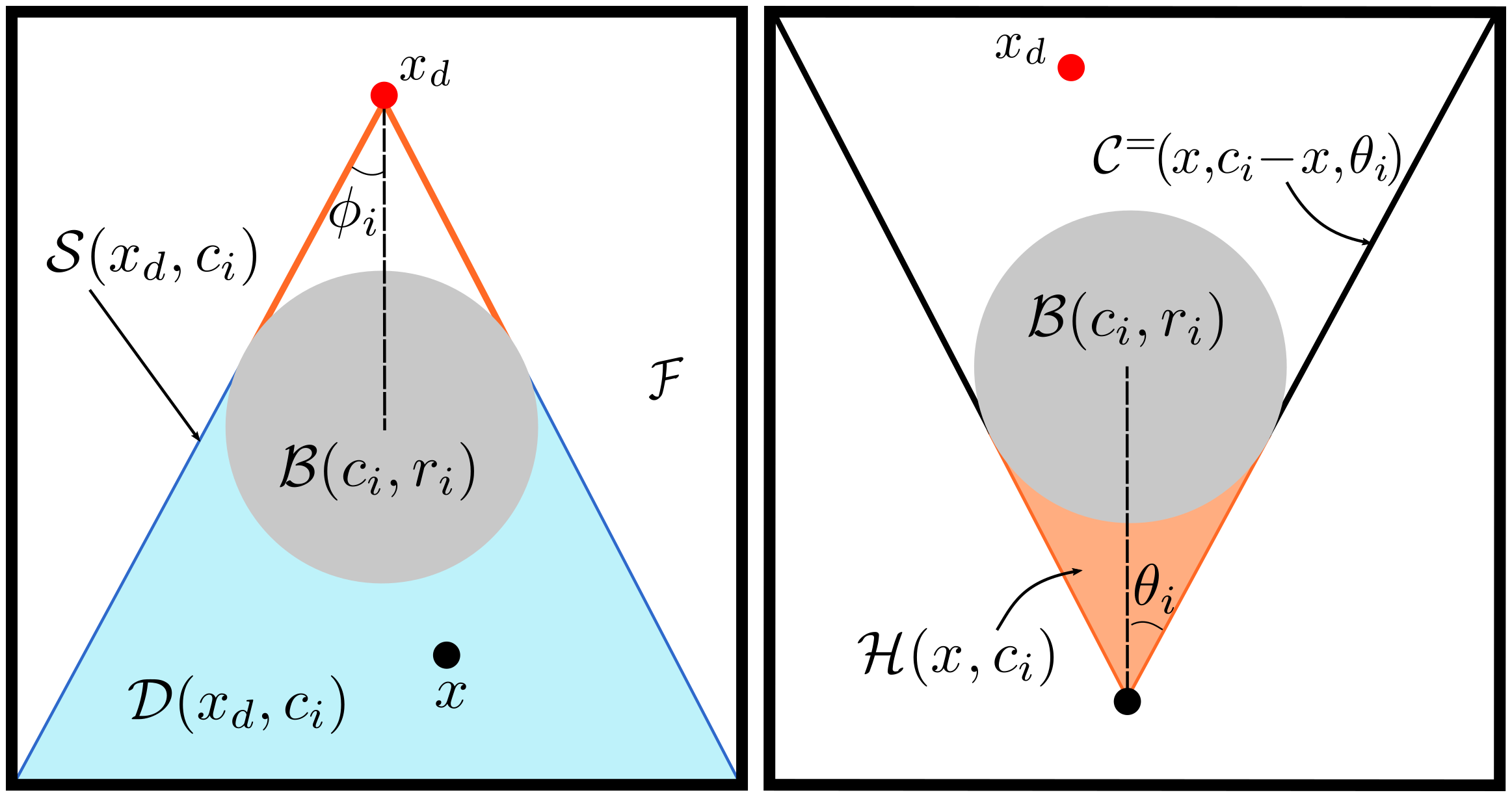
Figure 1: 2-D representation of the sets in Section IV.

Next, we classify the obstacles according to their visibility from the destination into different generations. An obstacle that can be fully seen from the destination is a first-generation obstacle (dark gray obstacles $\{1,2,3\}$ in Fig. 2). A second-generation obstacle can be partially seen from the destination and is partially included in the shadow regions of the first-generation obstacles (medium gray obstacles $\{4,5\}$ in Fig. 2). An obstacle is said to be of generation $j\geq 2$ if it is partially seen from the destination and is included in the shadow region of at least one obstacle of generation $j-1$. An obstacle that is completely hidden from the destination, whose shadow region is entirely included in the shadow regions of other obstacles, is classified as a zero-generation obstacle (light gray obstacles in Fig. 2). Now, we define the sets related to the obstacle classification as follows:

• The sub-shadow region of an obstacle $\mathcal{O}_{i}$ is defined as follows (see Fig. 2):

  $$\small\mathcal{D}^{j}(x_{d},c_{i}):=\mathcal{D}(x_{d},c_{i})\setminus\bigcup\limits_{l=1}^{j-1}\left[\bigcup\limits_{k\in J_{i}^{l}}\mathcal{D}^{l}(x_{d},c_{k})\right],$$ (14)

  for $j\geq 2$ where $J_{i}^{j}=\{k\in\left\{1,\dots,m\right\}|k\neq i\;\text{and}\;\mathcal{D}(x_{d},c_{i})\cap\mathcal{D}^{j}(x_{d},c_{k})\allowbreak\neq\varnothing\}$ is the set of the $j$-generation obstacles that include obstacle $i$ in their sub-shadow regions and $\mathcal{D}^{1}(x_{d},c_{i})=\mathcal{D}^{0}(x_{d},c_{i}):=\mathcal{D}(x_{d},c_{i})$.

• The blind set is a subset of $\mathcal{F}$ where there is no line of sight to the destination, and it is defined as

  $$\mathcal{BL}:=\bigcup\limits_{j=1}^{s}\left[\bigcup\limits_{i\in\mathcal{G}_{j}}\mathcal{D}^{j}(x_{d},c_{i})\right],$$ (15)

  where $\mathcal{G}_{j}$ is the set of obstacles of generation $j\in\{1,\dots,s\}$ and $s\leq m$ is the total number of generations in the workspace.

• The visible set is defined as the complement of the blind set with respect to the free space $\mathcal{VI}:=\mathcal{BL}^{c}_{\mathcal{F}}.$

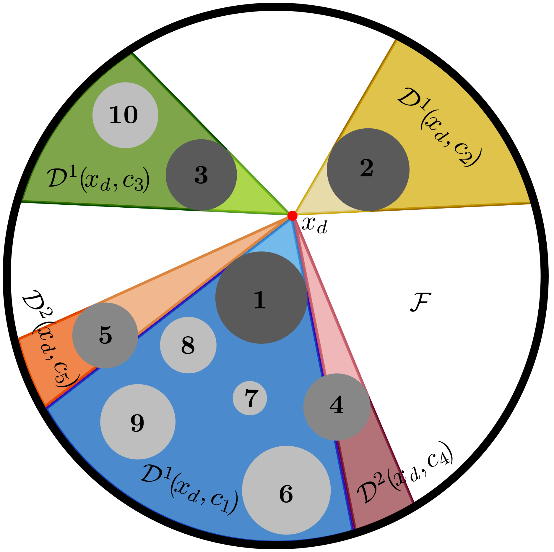
Figure 2: Sub-shadow regions of obstacles from different classes in a 2-D sphere world. First-generation obstacles are in dark gray, second-generation obstacles are in medium gray, and zero-generation obstacles are in light gray.

V Control Design

V-A Single Obstacle Case

We start by considering a single obstacle $\mathcal{O}_{i}$ and ignoring all others. We design a preliminary control law for the single obstacle case, which will be used as a baseline in the multiple obstacles case. First, in the case where the path is clear (i.e., $x$ belongs to the visible set $\mathcal{VI}$), the vehicle follows a straight line to the destination under the control law $u_{d}(x)=-\gamma(x-x_{d})$ where $\gamma\in\mathbb{R}_{>0}$. Next, in the case where the path is not clear (i.e., $x\in\mathcal{D}(x_{d},c_{i})$), we generate a control input (vehicle’s velocity) that is in the direction of the cone enclosing the obstacle $\mathcal{C}^{=}_{\mathcal{F}}(x,c_{i}-x,\theta_{i})$ while ensuring that the control input is equal to $u_{d}(x)$ at the exit set $\mathcal{S}(x_{d},c_{i})$. In particular, the direction of the control input should minimize the angle between the nominal control direction, given by $(x_{d}-x)$, and the set of all vectors parallel to the enclosing cone, i.e., the control input should belong to the set

$$\mathcal{U}_{1}(x):=\mathrm{arg}\min\limits_{v_{i}\in\mathcal{V}(c_{i}-x,\theta_{i})}\angle(x_{d}-x,v_{i}).$$ (16)

Moreover, to ensure continuity of the control input, we impose further that the control input belongs to the set

$$\mathcal{U}_{2}(x):=\{v\in\mathbb{R}^{n}:v=u_{d}(x),\;x\in\mathcal{S}(x_{d},c_{i})\}.$$ (17)

These two conditions can be written as follows

$$u(x)\in\mathcal{U}_{1}(x)\cap\mathcal{U}_{2}(x).$$ (18)

In the following lemma we show that the set $\mathcal{U}_{1}(x)\cap\mathcal{U}_{2}(x)$ is a singleton and we provide the unique solution.

Lemma 1

Set $\mathcal{U}_{1}(x)\cap\mathcal{U}_{2}(x)$ is a singleton and the unique element is given by

$$u(x)=\xi(u_{d}(x),x,i),$$ (19)

where $\xi:\mathbb{R}^{n}\times\mathbb{R}^{n}\times\mathbb{N}\setminus{0}\to\mathbb{R}^{n}$ is given by

$$\xi(u,x,i):=\frac{\sin(\beta_{i}(u,x))\sin^{-1}(\theta_{i}(x))}{\cos(\theta_{i}(x)-\beta_{i}(u,x))}\pi^{\parallel}(\bar{\xi})u,$$ (20)

with

$$\bar{\xi}:=\frac{\sin(\theta_{i}(x))u}{\sin(\beta_{i}(u,x))\|u\|}-\frac{\sin(\theta_{i}(x)-\beta_{i}(u,x))}{\sin(\beta_{i}(u,x))}\frac{(c_{i}-x)}{\|c_{i}-x\|},$$

$$\beta_{i}(u,x):=\angle(u,c_{i}-x)\leq\theta_{i}(x).$$

Proof:

See Appendix VIII-A. ∎

In other words, Lemma 1 shows that, when $x\in\mathcal{D}(x_{d},c_{i})$, the control $u(x)$ is a scaled parallel projection of the nominal controller $u_{d}(x)$ in the direction of $\bar{\xi}$ which represents a unit vector on the cone enclosing the obstacle. Finally, we obtain the following control strategy in the case of a single obstacle

$$u(x)=\begin{cases}\displaystyle u_{d}(x),&x\in\mathcal{VI},\\ \displaystyle\xi(u_{d}(x),x,i),&x\in\mathcal{D}(x_{d},c_{i}).\end{cases}$$ (21)

Note that, during the avoidance maneuver, the controller depends on three arguments: the nominal control $u_{d}(x)$, the current position of the vehicle $x$, and the obstacle index $i$. Moreover, the trajectory of the closed-loop system (9)-(21) generates an optimal obstacle avoidance maneuver as shown in the following lemma.

Lemma 2

The path generated by the closed-loop system (9)-(21) is the shortest path to the destination $x_{d}$ from every initial condition $x(0)\in\mathcal{F}\setminus\mathcal{L}_{d}(x_{d},c_{i})$ where $\mathcal{L}_{d}(x_{d},c_{i}):=\left\{q\in\mathcal{D}(x_{d},c_{i})|\;\;q=c_{i}+\delta(c_{i}-x_{d}),\;\delta\in\mathbb{R}_{>0}\right\}$.

Proof:

See Appendix VIII-B. ∎

V-B Multiple Obstacles Case

In the case of multiple obstacles and when $x\in\mathcal{BL}$, we proceed with multiple projections as described hereafter. When $x\in\mathcal{BL}$, there exist $j\in\{1,\dots,s\}$ and $i\in\mathcal{G}_{j}$ such that $x\in\mathcal{D}^{j}(x_{d},c_{i})$ (definition (15)). In this case, the obstacle $\mathcal{O}_{i}$ is the first to be considered, and $u_{d}(x)$ is projected onto its enclosing cone in a similar way as in (21). The resulting control vector is denoted by $u_{1}(x)$. The next obstacle to be considered is selected from the set of obstacles shadowed by obstacle $\mathcal{O}_{i}$ defined as $\mathcal{LO}_{i}(x):=\left\{k\in\left\{1,\dots,m\right\}\setminus\left\{i\right\}|\exists q\in\partial\mathcal{O}_{k},\,q\in\mathcal{H}(x,c_{i})\right\}$, see Fig. 3. Amongst obstacles in $\mathcal{LO}_{i}(x)$ that contain $u_{1}$ in their enclosing cones, we choose the closest in terms of the Euclidean distance to $\mathcal{O}_{i}$. If $\mathcal{LO}_{i}(x)=\varnothing$ or no obstacle contains $u_{1}$ in its enclosing cone, the path is free. Otherwise, $u_{1}$ will be considered as $u_{d}$ for the new selected obstacle and the same approach is followed to obtain $u_{2}$. We say that $\mathcal{O}_{i}$ is an ancestor to the selected obstacle and we repeat the selection and projection until the path is free (Fig. 3). The obstacles selected during the successive projections at a position $x$, are grouped in an ordered list $\mathcal{I}(x)\subset\mathbb{I}$ from the first obstacle ($\mathcal{O}_{i}$, such that $x\in\mathcal{D}^{j}(x_{d},c_{i})$) to the last one (obstacle involved in the last projection). Let $h(x)=\mathbf{card}(\mathcal{I}(x))$ be the number of required projections at position $x$. We define the bijection $\iota_{x}:\{1,\dots,h(x)\}\rightarrow\mathcal{I}(x)$ which associates to each projection $p\in\{1,\dots,h(x)\}$ the corresponding obstacle $\iota_{x}(p)\in\mathcal{I}(x)$. The set of positions involving obstacle $\iota_{x}(p)$ in the successive projections is called active region and defined as $\mathcal{AR}_{k}:=\left\{q\in\mathcal{BL}|k\in\mathcal{I}(q)\right\}$ with $k=\iota_{x}(p)$. To sum up, the intermediary control at a step $p\in\{1,\dots,h(x)\}$ and position $x\in\mathcal{AR}_{\iota_{x}(p)}$ is given by the recursive formula

$$u_{p}(x)=\xi(u_{p-1}(x),x,\iota_{x}(p)),$$ (22)

with $u_{0}(x)=u_{d}(x)$ and $\xi(\cdot,\cdot,\cdot)$ as defined in Lemma 1. Finally, the proposed control law is obtained by performing $h(x)$ successive projections and is given by

$$u(x)=\begin{cases}u_{d}(x),&x\in\mathcal{VI},\\ u_{h(x)}(x),&x\in\mathcal{BL}.\end{cases}$$ (23)

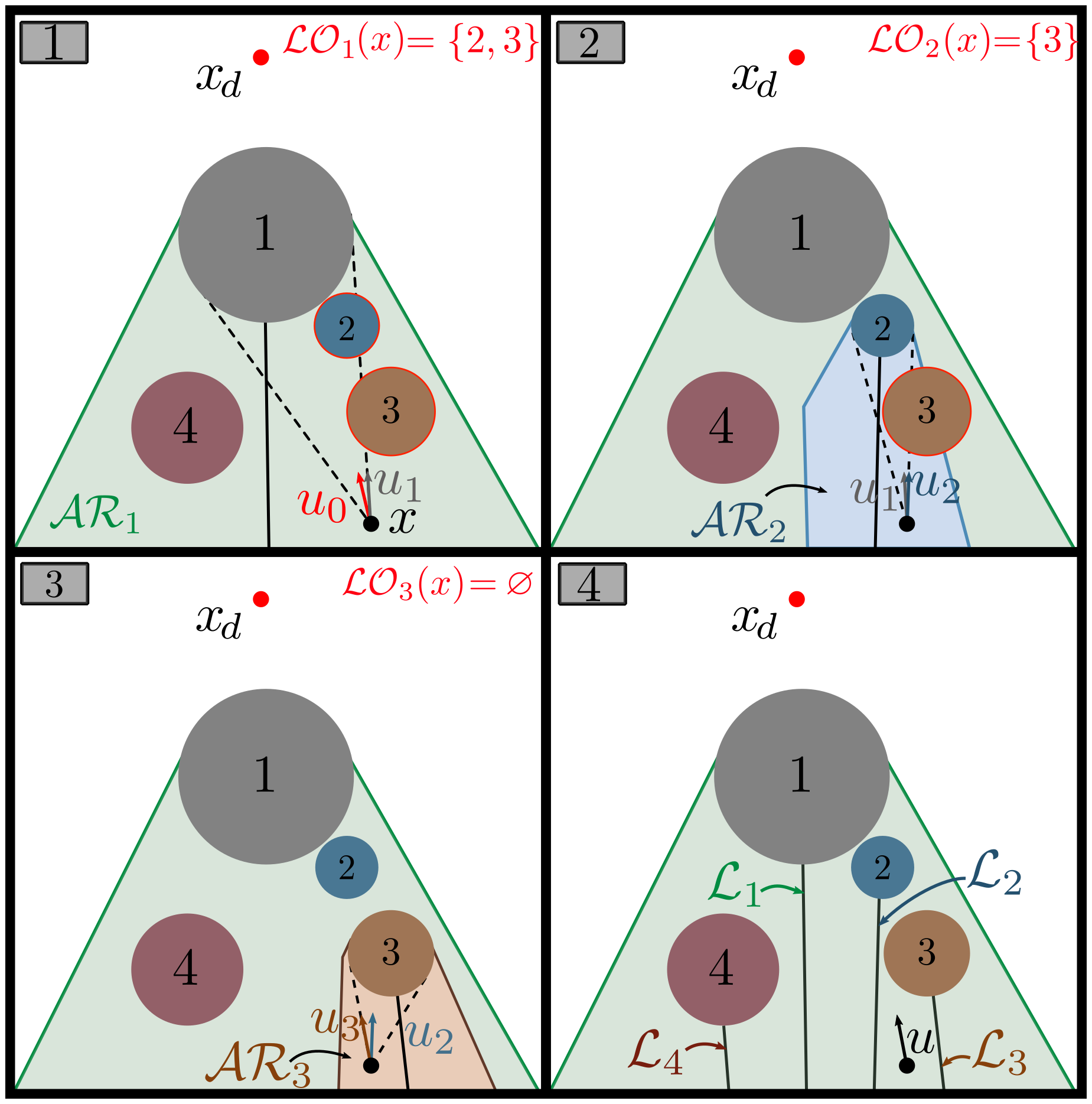
Figure 3: Successive projections of the control $u_{d}$ in a two-dimensional sphere world with four obstacles.

VI Safety and Stability Analysis

In this section, we analyse the safety and stability of the trajectories of the closed-loop system (9)-(23). Nagumo’s theorem ([16, 24]), offers an important tool to prove safety. One of the statements of this theorem is the one based on Bouligand’s tangent cones.

Definition 2

Given a closed set $\mathcal{K}$, the tangent cone to $\mathcal{K}$ at $x$ is $\mathcal{T}_{\mathcal{K}}(x):=\{z:\lim_{\tau\rightarrow 0}\mathrm{inf}\,\tau^{-1}d(x+\tau z,\mathcal{K})=0\}.$

In our case, when $x\in\mathring{\mathcal{F}}$, the tangent cone is the Euclidean space ($\mathcal{T}_{\mathcal{F}}(x)=\mathbb{R}^{n}$), and since the free space is a sphere world (smooth boundary), the tangent cone at its boundary is a half-space. Nagumo’s theorem guarantees, in a navigation problem, that the robot stays inside the free space $\mathcal{F}$. For this to be satisfied, the velocity vector $u(x)$ must point inside (or is tangent to) the free space [17]. In what follows, we rely on Nagumo’s theorem to prove the safety of the trajectories generated by our closed-loop system.

Theorem 1 (Safety)

Consider the closed set $\mathcal{F}$ described in (5) and the kinematic system (9) under the control law (23). Then, the closed-loop system (9)-(23) admits a unique solution for all $t\geq 0$, and the set $\mathcal{F}$ is forward invariant.

Proof:

See Appendix VIII-C. ∎

We define the central half-line associated to obstacle $i$

$$\mathcal{L}_{i}:=\left\{q\in\mathcal{AR}_{i}|\;\;\beta_{i}(u_{k-1},q)=0,k=\iota_{q}^{-1}(i)\right\}.$$ (24)

Let us look for the equilibria of the closed-loop system (9)-(23) by setting $u(x)=0$ in (23). From the first equation of (23), the equilibrium point is $x_{d}$. From (22), we can rewrite the control at step $p\in\{1,\dots,h(x)\}$ and position $x\in\mathcal{AR}_{\iota_{x}(p)}$, as $u_{p}=\sin(\beta_{i})\sin^{-1}(\theta_{i})\|u_{p-1}\|\bar{\xi}$ where $\iota_{x}(p)=i$. If we assume that $u_{p-1}\neq 0$, and since $\bar{\xi}\in\mathbb{S}^{n-1}$, $u_{p}=0$ if and only if $\beta_{i}=0$. Therefore, $u(x)=0$ if $x\in\mathcal{L}_{i}$, $i\in\mathbb{I}$. Finally, one can conclude that the set of equilibrium points of the system (9)-(23) is given by $\zeta:=\{x_{d}\}\cup(\cup_{i=1}^{m}\mathcal{L}_{i}).$ Now, to ensure that the undesired equilibria $\mathcal{L}_{i}$ have a repellency property, we assume the following.

Assumption 3

For any $i,k\in\mathbb{I}$, $i\neq k$, $\mathcal{L}_{k}\cap\mathcal{O}_{i}=\varnothing$.

Assumption 3 restricts the obstacles’ configurations in the workspace where no obstacle can intersect the central half-line of another obstacle. However, this will prevent the robot from getting trapped in a central half-line $\mathcal{L}_{k}$ when avoiding an obstacle $\mathcal{O}_{i}$.
In what follows, we present our main theorem:

Theorem 2

Consider the free space $\mathcal{F}\subset\mathbb{R}^{n}$ described in (5) and the closed-loop system (9)-(23). Under Assumptions 1, 2 and 3, the following statements hold:

• All trajectories converge to the set $\zeta=\{x_{d}\}\cup(\cup_{i=1}^{m}\mathcal{L}_{i})$.

• The set of equilibrium points $\cup_{i=1}^{m}\mathcal{L}_{i}$ is unstable and a repeller.

• The equilibrium point $x_{d}$ is locally exponentially stable on $\mathcal{F}$ and attractive from all $x(0)\in\mathcal{F}\setminus\cup_{i=1}^{m}\mathcal{L}_{i}$.

• From any initial position $x_{0}\in\mathcal{F}\setminus\cup_{i=1}^{m}\mathcal{L}_{i}$, the trajectory $x(t)$ generates a quasi-optimal obstacle avoidance maneuver.

Proof:

See Appendix VIII-D. ∎

Theorem 2 shows that the desired equilibrium point $x_{d}$ is almost globally asymptotically stable (since $\cup_{i=1}^{m}\mathcal{L}_{i}$ is Lebesgue measure zero) and that all trajectories of the closed-loop system are safe and quasi-optimal, in the sense of Definition 1. In the next section, we illustrate this optimality property in different scenarios.

VII Numerical simulation

To explore the extent of what our quasi-optimal avoidance maneuver can offer in terms of the shortest path in the multiple obstacle case, we compare the trajectories of our method (TP) to the shortest paths obtained with Dijkstra’s algorithm (DA) on a visibility tangent graph in five different and highly congested two-dimensional spaces where the first space is represented in Fig. 5a and the four other spaces are represented in Fig. 4. In each space, we take 100 random initial conditions, and we count the number of perfect matching of the paths. The summarized results in Table I show a high rate of success, while the failures of taking the shortest path can be explained through the fact that, at each instant, our approach considers the set $\mathcal{I}(x)$ engaged in the nested successive projections that may lead to a non-optimal path. Compared to Dijkstra’s algorithm, which takes the shortest path from the visibility tangent graph that considers all the obstacles.
To visualize the properties of our approach, we consider thirteen obstacles in two different scenarios. In the first scenario, we assume that the robot evolves in $\mathbb{R}^{2}$ where the destination $x_{d}=[0\;0]^{\top}$, while the second scenario is in $\mathbb{R}^{3}$ and the goal is $x_{d}=[0\;0\;0]^{\top}$. In both cases, we consider fifteen different initial positions. A comparison of our approach with the navigation function approach (NF) [6] and the separating hyperplane approach (SH) [13] is established in the two-dimensional space. The simulation results in Fig. 5 show that all the trajectories generated by our control are safe and converge to the red target. In addition, Fig. 5a shows the superiority of our approach over the two other methods in terms of the length of the generated collision-free paths, where it generates the same paths as DA.

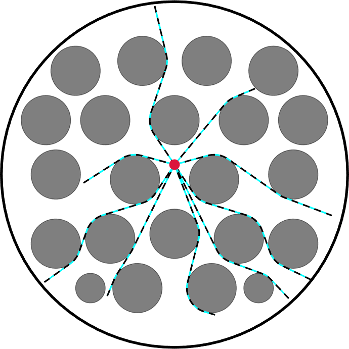
(a)

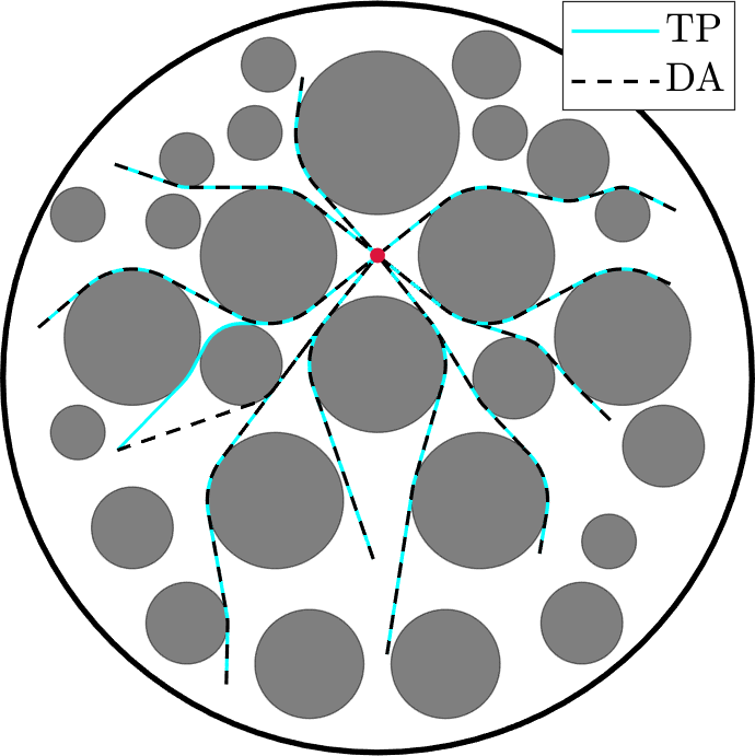
(b)

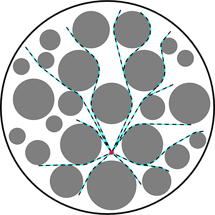
(c)

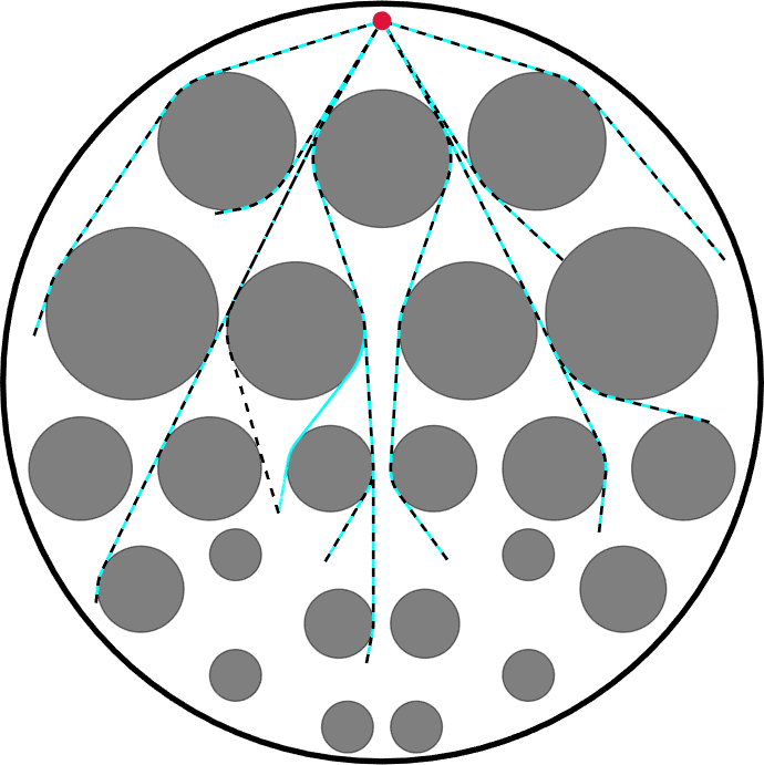
(d)

Figure 4: Some samples among 100 tests between (DA) and our approach (TP) in 4 different spaces.

TABLE I: Success rate of the perfect match between the paths generated by our control and the paths of DA.

Space 1	Space 2	Space 3	Space 4	Space 5
96$\%$	98$\%$	93$\%$	97$\%$	97$\%$

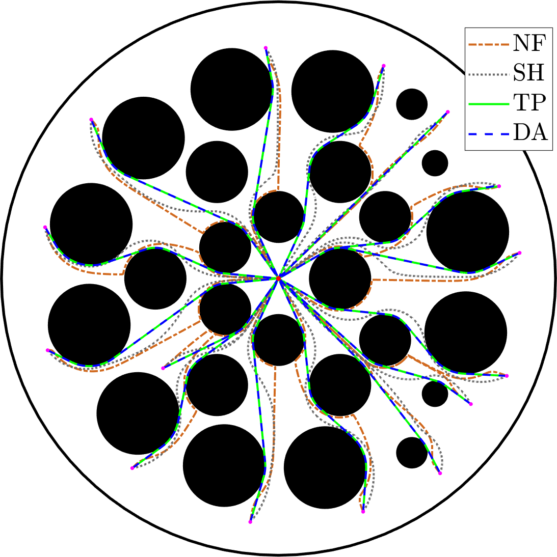
(a)

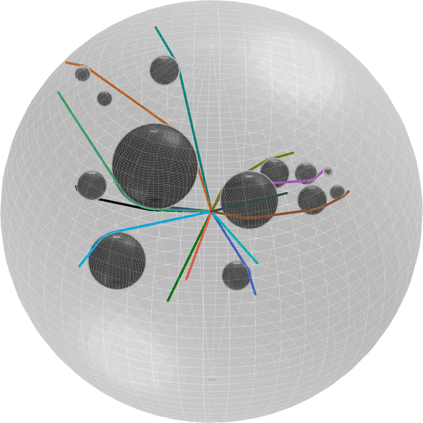
(b)

Figure 5: Robot safe navigation from fifteen different initial positions. Fig. (a) is a comparison between our method TP, SH, NF, and DA in a two-dimensional sphere world, while Fig (b) only shows the performance of our approach in a three-dimensional sphere world.

VIII Conclusion

We have proposed a quasi-optimal continuous feedback control strategy, with almost global asymptotic stability guarantees, for the autonomous navigation problem in an $n$-dimensional sphere world. The proposed strategy consists in steering the robot tangentially to the blocking obstacles through successive projections of the nominal control onto the obstacles enclosing cones. Consequently, the intermediary obstacle avoidance maneuvers are optimal, resulting in a quasi-optimal overall collision-free path. We recognize that the price to pay to obtain the claimed results in the paper is a somewhat restrictive assumption on the obstacles configuration (Assumption 3) that needs to be relaxed in our future investigations. Extending the proposed approach to arbitrarily shaped obstacles, with global asymptotic stability guarantees, is another interesting problem that will be the main focus of our future work.

APPENDIX

VIII-A Proof of Lemma 1

Minimizing the angle $\angle(x_{d}-x,v_{i})$ is equivalent to minimizing the cost function $g(v_{i})=1-V_{d}^{\top}\frac{v_{i}}{\|v_{i}\|}$ with $V_{d}=(x_{d}-x)/\|x_{d}-x\|$ under the constraint $\Gamma(v_{i})=\frac{v_{i}^{\top}V_{ci}}{\|v_{i}\|}-\cos(\theta_{i})=0$ with $V_{ci}=(c_{i}-x)/\|c_{i}-x\|$. We define the Lagrangian associated to the optimization problem (16) by $L_{\lambda}(v_{i})=g(v_{i})-\lambda\Gamma(v_{i})$ where $\lambda$ is the Lagrange multiplier. The optimum is the solution of $\nabla_{v_{i},\lambda}L_{\lambda}(v_{i})=0$ which gives

$$\pi^{\bot}(v_{i})(V_{d}+\lambda V_{ci})=0,\quad\frac{v_{i}^{\top}V_{ci}}{\|v_{i}\|}-\cos(\theta_{i})=0.$$ (25)

From the first equation, we have $v_{i}=\alpha(V_{d}+\lambda V_{ci})$ for some $\alpha\in\mathbb{R}$. Substituting this into (25) and then , we can solve for $\lambda$ and find

$$\lambda_{1,2}=-\frac{\sin(\theta_{i}\pm\beta_{i})}{\sin(\theta_{i})},$$ (26)

Therefore, we obtain two vectors $v_{i}^{1}$ and $v_{i}^{2}$ such that

$$v_{i}^{1,2}=\alpha_{1,2}\left(V_{d}-\frac{\sin(\theta_{i}\pm\beta_{i})}{\sin(\theta_{i})}V_{ci}\right),$$ (27)

where $\alpha_{1}\leq 0$ and $\alpha_{2}\geq 0$. The value of $g$ at the two solutions is as follows:

$$\small g(v_{i}^{1})=1+\cos(\theta_{i}+\beta_{i}),\;g(v_{i}^{2})=1-\cos(\theta_{i}-\beta_{i}),$$

and $g(v_{i}^{1})-g(v_{i}^{2})=2\cos(\theta_{i})\cos(\beta_{i})\geq 0$ which implies that

$$\mathcal{U}_{1}(x)=\{\alpha_{2}(V_{d}-\sin^{-1}(\theta_{i})\sin(\theta_{i}-\beta_{i})V_{ci})|\;\alpha_{2}\geq 0\}.$$ (28)

When $x\in\mathcal{S}(x_{d},c_{i})$, $\theta_{i}=\beta_{i}$ and for all $v_{i}\in\mathcal{U}_{1}$, $v_{i}\in\mathcal{U}_{2}$. Therefore, $\alpha_{2}V_{d}=u_{d}(x)$ which implies that $\alpha_{2}=\gamma\|x_{d}-x\|$. One can conclude that the set $\mathcal{U}_{1}\cap\mathcal{U}_{2}$ is a singleton and the unique solution is given by

$$\small u(x) =\gamma\|x_{d}-x\|\left(V_{d}-\frac{\sin(\theta_{i}-\beta_{i})}{\sin(\theta_{i})}V_{ci}\right)=\xi(u_{d}(x),x,i),$$

where the last equation is obtained after some straightforward manipulation.

VIII-B Proof of Lemma 2

Let $x(0)\in\mathcal{F}\setminus\mathcal{L}_{d}(x_{d},c_{i})$. Then we have two situations. First, when $x(0)\in\mathcal{VL}$, the trajectory $x(t)$ is a line-segment which is the closest path. Now, when $x(0)\in\mathcal{D}(x_{d},c_{i})$, there are two types of possible trajectories: trajectories inside the enclosing cone $\mathcal{C}^{\leq}_{\mathcal{F}}(x,c_{i}-x,\theta_{i})$ and trajectories outside this cone. We show that the trajectory generated by the closed-loop system (9)-(21) on the enclosing cone $\mathcal{C}^{=}_{\mathcal{F}}(x,c_{i}-x,\theta_{i})$ has the minimum length. For the first type of trajectory, we only consider the ones between the line segment $\mathcal{L}_{s}(x(0),x_{d})$ and the closest tangent to it (green segment in Fig. 6) among the cone enclosing the obstacle (the red trajectory in Fig. 6 is an example). All these trajectories will merge with our trajectory, which is on the closest tangent (as shown in Lemma 1), at the intersection point of the tangent with the obstacle. Since, before the intersection point, our trajectory is a line segment, we can conclude that it is the shortest path. The best that can be achieved outside the cone for a smooth trajectory is a dilated version of our trajectory (larger radius of curvature) which is longer than ours (black path in Fig. 6).

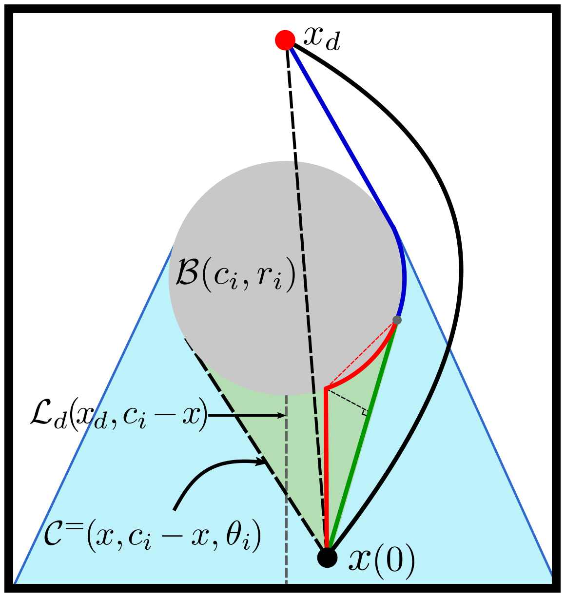
Figure 6: Shortest path in a single-obstacle sphere world.

VIII-C Proof of Theorem 1

First we prove that the closed-loop system admits a unique solution. The control is Lipschitz on $\mathcal{VI}$ since $u(x)=u_{d}(x)$ is continuously differentiable. When $x\in\mathcal{BL}$, for simplicity, we denote $\sin(\theta_{\iota_{x}(p)}(q)-\beta_{\iota_{x}(p)}(u_{p-1}(x),q))$ by $s_{\iota_{x}(p)}^{s}(q)$ and $\frac{\sin(\beta_{\iota_{x}(p)}(u_{p-1}(x),q))}{\sin(\theta_{\iota_{x}(p)}(q))}$ by $s_{\iota_{x}(p)}^{d}(q)$ where $p\in\{1,\dots,h(x)\}$. After manipulation, the control (23) can be expressed as $u(x)=u_{d}(x)-\gamma\|x-x_{d}\|\sum\limits_{p=1}^{h(x)}\prod\limits_{k=1}^{p-1}s_{\iota(k)}^{d}(x)\frac{s_{\iota(p)}^{s}(x)}{r_{\iota(p)}}(c_{\iota(p)}-x)$, and we prove that it is one-sided Lipschitz as follows:

$$\begin{split}&\left(u(x)-u(y)\right)^{\top}(x-y)=-\gamma\|x-y\|^{2}\\ &-\gamma\|x_{d}-x\|\sum\limits_{p=1}^{h(x)}\prod\limits_{k=1}^{p-1}s_{\iota(k)}^{d}(x)\frac{s_{\iota(p)}^{s}(x)}{r_{\iota(p)}}(c_{\iota(p)}-x)^{\top}(x-y)\\ &+\gamma\|x_{d}-y\|\sum\limits_{p=1}^{h(y)}\prod\limits_{k=1}^{p-1}s_{\iota(k)}^{d}(y)\frac{s_{\iota(p)}^{s}(y)}{r_{\iota(p)}}(c_{\iota(p)}-y)^{\top}(x-y)\\ &\leq-\gamma\|x-y\|^{2}\\ &+\gamma\|x_{d}-x\|\|x-y\|\sum\limits_{p=1}^{h(x)}\prod\limits_{k=1}^{p-1}s_{\iota(k)}^{d}(x)\frac{s_{\iota(p)}^{s}(x)}{r_{\iota(p)}}\|c_{\iota(p)}-x\|\\ &+\gamma\|x_{d}-y\|\|x-y\|\sum\limits_{p=1}^{h(y)}\prod\limits_{k=1}^{p-1}s_{\iota(k)}^{d}(y)\frac{s_{\iota(p)}^{s}(y)}{r_{\iota(p)}}\|c_{\iota(p)}-y\|.\end{split}$$

Note that $\forall x\in\mathcal{BL}$ and $\forall p\in\{1,\dots,h(x)\}$, $0\leq s_{\iota(p)}^{d}(x)\leq 1$, $0\leq s_{\iota(p)}^{s}(x)\leq 1$, $\|c_{\iota(p)}-x\|\leq 2r_{0}-r_{\iota(p)}$ and $\|x_{d}-x\|\leq 2r_{0}$, which implies that there exists $M>0$ such that $\|x_{d}-x\|\sum_{p=1}^{h(x)}\frac{\|c_{\iota(p)}-x\|}{r_{\iota(p)}}\leq M\|x-y\|$. Therefore,

$$\begin{split}&\left(u(x)-u(y)\right)^{\top}(x-y)\leq-\gamma\|x-y\|^{2}+\\ &\qquad\gamma M_{1}\|x-y\|^{2}+\gamma M_{2}\|x-y\|^{2}\\ &\quad\leq\gamma(-1+M_{1}+M_{2})\|x-y\|^{2}\leq L\|x-y\|^{2}.\end{split}$$

One can take $L=\gamma(-1+M_{1}+M_{2})$ where $M_{1}>0$, $M_{2}>0$ and $M_{1}+M_{2}>1$. The control (23) is one-sided Lipschitz [25] when $x\in\mathcal{BL}($ and is Lipschitz when $x\in\mathcal{VI}$. Thus, according to [25, Proposition 2], the closed-loop system (9)-(23) has a unique solution for all $x(0)\in\mathcal{F}$. Now, we prove forward invariance using Nagumo’s theorem. We only need to verify Nagumo’s condition at the free space boundary as it is trivially met when $x\in\mathring{\mathcal{F}}$ where $\mathcal{T}_{\mathcal{F}}(x)=\mathbb{R}^{n}$. Since the free space is a sphere world, the tangent cone on its boundary is the half-space $\mathcal{C}^{\leq}_{\mathbb{R}^{n}}(x,-x,\frac{\pi}{2})$ when $x\in\partial\mathcal{W}$ and $\mathcal{C}^{\geq}_{\mathbb{R}^{n}}(x,c_{i}-x,\frac{\pi}{2})$ when $x\in\partial\mathcal{O}_{i}$. We consider an obstacle $\mathcal{O}_{i}$ and verify Nagumo’s condition in three regions of the free space.
In the first region, When $x\in\partial\mathcal{W}$, $\mathcal{T}_{\mathcal{F}}(x)=\mathcal{C}^{\leq}_{\mathbb{R}^{n}}(x,-x,\frac{\pi}{2})$ and two sub-regions must be considered.

• $x\in\partial\mathcal{W}\cap\partial\mathcal{BL}$: Since $u(x)\in\mathcal{C}^{=}_{\mathcal{F}}(x,c_{i}-x,\theta_{i})$ and $\mathcal{C}^{=}_{\mathcal{F}}(x,c-x,\theta)\subseteq\mathcal{C}^{\leq}_{\mathbb{R}^{n}}(x,-x,\frac{\pi}{2})$, we conclude that $u(x)\in\mathcal{T}_{\mathcal{F}}(x)$.

• $x\in\partial\mathcal{W}\setminus\partial\mathcal{BL}$: Since $u_{d}(x)\in\mathcal{F}$ and $\mathcal{F}\subseteq\mathcal{C}^{\leq}_{\mathbb{R}^{n}}(x,-x,\frac{\pi}{2})$, we conclude that $u(x)=u_{d}(x)\in\mathcal{T}_{\mathcal{F}}(x)$.

In the second region, $x\in\partial\mathcal{O}_{i}\cap\mathcal{AR}_{i}$ and $\mathcal{T}_{\mathcal{F}}(x)=\mathcal{C}^{\geq}_{\mathbb{R}^{n}}(x,c_{i}-x,\frac{\pi}{2})$. Since $u(x)\in\mathcal{C}^{=}_{\mathbb{R}^{n}}(x,c_{i}-x,\frac{\pi}{2})\subset\mathcal{C}^{\geq}_{\mathbb{R}^{n}}(x,c_{i}-x,\frac{\pi}{2})$, one concludes that $u(x)\in\mathcal{T}_{\mathcal{F}}(x)$. Finally, in the last region, $x\in\partial\mathcal{O}_{i}\setminus\mathcal{AR}_{i}$ and $\mathcal{T}_{\mathcal{F}}(x)=\mathcal{C}^{\geq}_{\mathbb{R}^{n}}(x,c_{i}-x,\frac{\pi}{2})$. Since $x\notin\mathcal{AR}_{i}$, $\forall p\in\{0,\cdots,h(x)\}$, obstacle $\mathcal{O}_{i}$ is not selected in the successive projections $(\iota_{x}(p)\neq i)$ and $u_{p}(x)\notin\mathcal{C}^{\leq}_{\mathbb{R}^{n}}(x,c_{i}-x,\frac{\pi}{2})$. Therefore, $u(x)$ must be in the complement of the enclosing cone to the obstacle $\mathcal{O}_{i}$. Thus, one can conclude that $u(x)\in\mathcal{C}^{\geq}_{\mathbb{R}^{n}}(x,c_{i}-x,\frac{\pi}{2})=\mathcal{T}_{\mathcal{F}}(x)$.

Since $\forall x\in\mathcal{F},\;\;u(x)\in\mathcal{T}_{\mathcal{F}}(x)$ and the solution of the closed-loop system (9)-(23) is unique, it follows that the free space $\mathcal{F}$ is positively invariant and the closed-loop system (9)-(23) is safe.

VIII-D Proof of Theorem 2

Four points must be demonstrated, safety of the system, quasi-optimality of the avoidance maneuver, stability of the destination $x_{d}$ and instability of the remaining equilibria.
First, we start by proving the safety of our system. By virtue of Theorem 1, the closed-loop system (9)-(23) is safe for all $x\in\mathcal{F}$.
Next, we prove the instability of the equilibria $\mathcal{L}_{i}$ with $i\in\mathbb{I}$. Consider an obstacle $\mathcal{O}_{i}$ and the set of its ancestors $\mathcal{AN}_{i}\subset\{0,\dots,m\}$ where $i\notin\mathcal{AN}_{i}$ and the element $0$ refers to the destination. Each ancestor generates a subset $\mathcal{AR}_{i}^{k}$ of the active shadow region $\mathcal{AR}_{i}$ where $\mathcal{AR}_{i}^{k}\cap\mathcal{AR}_{i}^{j}=\varnothing$ for all $k,j\in\mathcal{AN}_{i}$ and $k\neq j$, and $\mathcal{AR}_{i}=\bigcup\limits_{k\in\mathcal{AN}_{i}}\mathcal{AR}_{i}^{k}$. The subset generated by the ancestor responsible for the creation of the central half-line $\mathcal{L}_{i}$ is denoted by $\mathcal{AR}_{i}^{*}$. We consider the set of equilibrium points $\mathcal{L}_{i}$ where $i\in\mathbb{I}$ and we define the extended central half-line $\mathcal{L}_{i}^{e}:=\left\{q\in\mathcal{W}|q=c_{i}+\delta\frac{y-c_{i}}{\|y-c_{i}\|}\,,y\in\mathcal{L}_{i}\,,\delta\in\mathbb{R}_{>0}\right\}$. We also define the cylinder inside $\mathcal{AR}_{i}^{*}$ by $\mathcal{CY}_{i}(e_{i},\epsilon_{i}):=\left\{q\in\mathcal{AR}_{i}^{*}|\,d\left(q,\mathcal{L}_{i}^{e}\right)<e_{i}\,\text{and}\,\|q-c_{i}\|<\epsilon_{i},\,e_{i},\epsilon_{i}\in\mathbb{R}_{>0}\right\}$, where $\epsilon_{i}$ is such that for all $x\in\mathcal{CY}_{i}(e_{i},\epsilon_{i})$, the considered obstacle $\mathcal{O}_{i}$ is the last on the successive projection, i.e., $\forall x\in\mathcal{CY}_{i}(e_{i},\epsilon_{i}),\,\iota_{x}(h(x))=i$. We also define the set $U:=\mathcal{CY}_{i}(e_{i},\epsilon_{i})\setminus\mathcal{L}_{i}$. Let the equilibrium point $\bar{x}_{i}\in\mathcal{L}_{i}$ and $V_{1}(x)=1-\frac{(\bar{x}_{i}-c_{i})^{\top}}{r_{i}}\frac{(x-c_{i})}{||x-c_{i}||}$ where $V_{1}(\bar{x}_{i})=0$ and $V_{1}(x)>0$ for all $x\in U$.

$$\dot{V}_{1}(x) =\frac{\partial V_{1}(x)}{\partial x}^{\top}\dot{x}=-\frac{(\bar{x}_{i}-c_{i})^{\top}}{r_{i}}J_{x}\left(\frac{(x-c_{i})}{||x-c_{i}||}\right)u(x)$$

$$=-K\bar{V}^{\top}_{ci}\pi^{\bot}(V_{ci})\bar{\xi},$$

where $K=\frac{\|u(x)\|\|\bar{x}_{i}-c_{i}\|}{r_{i}||x-c_{i}||}>0$, $V_{ci}=\frac{(c_{i}-x)}{\|c_{i}-x\|}$, $\bar{V}_{ci}=\frac{(\bar{x}_{i}-c_{i})}{\|\bar{x}_{i}-c_{i}\|}$ and $\bar{\xi}=\frac{\sin(\theta_{i})u_{h(x)-1}}{\sin(\beta_{i})\|u_{h(x)-1}\|}-\frac{\sin(\theta_{i}-\beta_{i})}{\sin(\beta_{i})}V_{ci}$. Recall that the control, at position $x\in\mathcal{BL}$, is written as $u(x)=u_{h(x)}(x)=\sin(\beta_{i})\sin^{-1}(\theta_{i})\|u_{h(x)-1}\|\bar{\xi}$ with $i=\iota_{x}(h(x))$. Then, the vectors $u_{h(x)}$, $u_{h(x)-1}$ and $V_{ci}$ are on the same $2$D plane. Moreover, the central half-line $\mathcal{L}_{i}$ is generated by the overlap between $V_{ci}$ and $u_{h(x)-1}/\|u_{h(x)-1}\|$ when $x\in\mathcal{AR}_{i}^{*}$. Therefore, the vectors $u_{p}(x)$, $u_{h(x)-1}(x)$, $V_{ci}$ and the central half-line $\mathcal{L}_{i}$ are on the same plane. Similarly, the vectors $\bar{\xi}$, $V_{ci}$ and $\bar{V}_{ci}$ are on same plane, and thus,

$$\dot{V}_{1}(x) =-K\left(\cos(\sigma_{i})-\cos(\theta_{i})\cos(\sigma_{i}+\theta_{i})\right),$$

$$=K\left(\cos(\sigma_{i})\sin^{2}(\theta_{i})+\cos(\theta_{i})\sin(\sigma_{i})\sin(\theta_{i})\right)$$

$$=K\sin(\theta_{i})\sin(\sigma_{i}-\theta_{i}),$$

where $\frac{\pi}{2}<\angle(\bar{V}_{ci},\bar{\xi})=\sigma_{i}\leq\pi$ and $0<\sigma_{i}-\theta_{i}<\pi$.
$\dot{V_{1}}(\bar{x}_{i})=0$ and $\dot{V_{1}}(x)>0$ for all $x\in U$. According to Chetaev’s theorem [26, Theorem 4.3], the equilibrium point $\bar{x}_{i}$ is unstable, and for any $x_{0}\in U$, $x(t)$ must leave $U$ from all directions else than the surface of the obstacle (due to the safety of the system). Moreover, considering assumption 3 and that the control $u(x)$ is tangent to the last obstacle $\iota(h(x))$, we can conclude that $x(t)$ must leave the active shadow region of the last obstacle. Therefore, any equilibrium $\bar{x}_{i}\in\mathcal{L}_{i}$ is unstable and a repeller, and the blind set has the following property:

$$\exists t^{*}\in\mathbb{R}_{>0},\;\forall x(0)\in\mathcal{BL}\setminus\bigcup\limits_{i=1}^{m}\mathcal{L}_{i},\;x(t^{*})\notin\mathcal{BL}.$$ (29)

Now we prove the stability of the $x_{d}$. We consider the equilibrium point $x_{d}$ and the positive definite function $V_{2}(x)=\frac{1}{2}||x-x_{d}||^{2}$. The closed-loop system (9)-(23) reduces to $\dot{x}=-\gamma(x-x_{d})$ When $x\in\mathcal{VI}$. Therefore, $\dot{V}_{2}(x)=-\gamma||x-x_{d}||^{2}<0$. We can conclude that the destination is locally exponentially stable and almost globally asymptotically stable using the property (29). Finally, we show the quasi-optimality of our obstacle avoidance maneuver. Since the control input (23) is a composition of the projection from Lemma 1, which generates the shortest path for a considered obstacle, according to Lemma 2, the trajectory $x(t)$ of the closed-loop system (9)-(23) generates a quasi-optimal obstacle avoidance maneuver, for $\varepsilon=0$, as per Definition 1.

References

• [1] E. W. Dijkstra, “A note on two problems in connexion with graphs,” Numerische Mathematik, vol. 1, pp. 269–271, 1959.
• [2] P. E. Hart, N. J. Nilsson, and B. Raphael, “A formal basis for the heuristic determination of minimum cost paths,” IEEE Transactions on Systems Science and Cybernetics, vol. 4, no. 2, pp. 100–107, 1968.
• [3] V. Lumelsky and A. Stepanov, “Dynamic path planning for a mobile automaton with limited information on the environment,” IEEE Transactions on Automatic Control, vol. 31, no. 11, pp. 1058–1063, 1986.
• [4] V. Lumelsky and T. Skewis, “Incorporating range sensing in the robot navigation function,” IEEE Transactions on Systems, Man, and Cybernetics, vol. 20, no. 5, pp. 1058–1069, 1990.
• [5] O. Khatib, “Real time obstacle avoidance for manipulators and mobile robots,” The International Journal of Robotics Research, vol. 5, no. 1, pp. 90–99, 1986.
• [6] D. E. Koditchek and E. D. Rimon, “Robot Navigation Functions on Manifolds with Boundary,” Advances in Applied Mathematics, vol. 11, pp. 412–442, 1990.
• [7] E. D. Rimon and D. E. Koditchek, “The construction of analytic diffeomorphisms for exact robot navigation on star worlds,” Transactions of the American Mathematical Society, vol. 327, no. 1, pp. 71–116, 1991.
• [8] E. D. Rimon and D. E. Koditchek, “Exact Robot Navigation Using Artificial Potential Functions,” IEEE Transactions on Robotics and Automation, vol. 8, no. 5, pp. 501–518, 1992.
• [9] S. G. Loizou, “The navigation transformation: Point worlds, time abstractions and towards tuning-free navigation,” in 2011 19th Mediterranean Conference on Control Automation (MED), pp. 303–308, 2011.
• [10] N. Constantinou and S. G. Loizou, “Robot navigation on star worlds using a single-step navigation transformation,” in 2020 59th IEEE Conference on Decision and Control (CDC), pp. 1537–1542, 2020.
• [11] S. Paternain, D. E. Koditschek, and A. Ribeiro, “Navigation functions for convex potentials in a space with convex obstacles,” IEEE Transactions on Automatic Control, vol. 63, no. 9, pp. 2944–2959, 2018.
• [12] S. G. Loizou and E. D. Rimon, “Correct-by-construction navigation functions with application to sensor based robot navigation,” arXiv, 2021.
• [13] O. Arslan and D. E. Koditschek, “Sensor-based reactive navigation in unknown convex sphere worlds,” The International Journal of Robotics Research, vol. 38, no. 2-3, pp. 196–223, 2019.
• [14] V. G. Vasilopoulos and D. E. Koditschek, “Reactive Navigation in Partially Known Non-Convex Environments,” in 13th International Workshop on the Algorithmic Foundations of Robotics (WAFR), 2018.
• [15] V. G. Vasilopoulos, G. Pavlakos, K. Schmeckpeper, K. Daniilidis, and D. E. Koditschek, “Reactive navigation in partially familiar planar environments using semantic perceptual feedback,” ArXiv, vol. abs/2002.08946, 2020.
• [16] M. Nagumo, “Über die lage der integralkurven gewöhnlicher differentialgleichungen,” Proceedings of the Physico-Mathematical Society of Japan. 3rd Series, vol. 24, pp. 551–559, 1942.
• [17] S. Berkane, “Navigation in unknown environments using safety velocity cones,” in 2021 American Control Conference (ACC), pp. 2336–2341, 2021.
• [18] A. D. Ames, J. W. Grizzle, and P. Tabuada, “Control barrier function based quadratic programs with application to adaptive cruise control,” in 53rd IEEE Conference on Decision and Control, pp. 6271–6278, 2014.
• [19] A. D. Ames, X. Xu, J. W. Grizzle, and P. Tabuada, “Control barrier function based quadratic programs for safety critical systems,” IEEE Transactions on Automatic Control, vol. 62, no. 8, pp. 3861–3876, 2017.
• [20] R. Sanfelice, M. Messina, S. Emre Tuna, and A. Teel, “Robust hybrid controllers for continuous-time systems with applications to obstacle avoidance and regulation to disconnected set of points,” in 2006 American Control Conference, pp. 6 pp.–, 2006.
• [21] S. Berkane, A. Bisoffi, and D. V. Dimarogonas, “Obstacle avoidance via hybrid feedback,” IEEE Transactions on Automatic Control, vol. 67, no. 1, pp. 512–519, 2022.
• [22] M. Sawant, S. Berkane, I. Polushin, and A. Tayebi, “Hybrid feedback for autonomous navigation in environments with arbitrary convex obstacles,” arXiv:2111.09380, 2022.
• [23] S. Berkane, A. Bisoffi, and D. V. Dimarogonas, “A hybrid controller for obstacle avoidance in an $n$-dimensional euclidean space,” in 2019 18th European Control Conference (ECC), pp. 764–769, 2019.
• [24] F. Blanchini and S. Miani, Set-Theoretic Methods in Control. Birkhäuser Basel, 1st ed., 2007.
• [25] J. Cortes, “Discontinuous dynamical systems,” IEEE Control Systems Magazine, vol. 28, no. 3, pp. 36–73, 2008.
• [26] H. K. Khalil, Nonlinear systems; 3rd ed. Upper Saddle River, NJ: Prentice-Hall, 2002.