Uncertainty Injection: A Deep Learning Method for Robust Optimization

Abstract

This paper proposes a paradigm of uncertainty injection for training deep learning model to solve robust optimization problems. The majority of existing studies on deep learning focus on the model learning capability, while assuming the quality and accuracy of the inputs data can be guaranteed. However, in realistic applications of deep learning for solving optimization problems, the accuracy of inputs, which are the problem parameters in this case, plays a large role. This is because, in many situations, it is often costly or sometime impossible to obtain the problem parameters accurately, and correspondingly, it is highly desirable to develop learning algorithms that can account for the uncertainties in the input and produce solutions that are robust against these uncertainties. This paper presents a novel uncertainty injection scheme for training machine learning models that are capable of implicitly accounting for the uncertainties and producing statistically robust solutions. We further identify the wireless communications as an application field where uncertainties are prevalent in problem parameters such as the channel coefficients. We show the effectiveness of the proposed training scheme in two applications: the robust power loading for multiuser multiple-input-multiple-output (MIMO) downlink transmissions; and the robust power control for device-to-device (D2D) networks.

I Introduction

Deep learning has achieved excellent results in a variety of different optimization tasks, such as the inference problems [2, 3, 4] and the generative modeling problems [5, 6, 7]. Although the traditional domain of deep learning has been for applications in which the optimization problems do not admit explicit mathematical models, several recent advances have also shown the promise of deep learning in solving non-convex optimization problems for which explicit mathematical formulations are available, e.g., [8, 9, 10]. This paper focuses on this latter class of problems in which a deep learning model is trained to take the parameters of the mathematical optimization problem as the input and to output the optimized solution of the problem. Specifically, we focus on how to train the model to achieve robustness against uncertainty in the problem parameters.

While most of the deep learning literature focuses on the learning performance of the neural network on a given dataset where the availability of high-quality input data is assumed, in many realistic applications, the uncertainties are inevitably part of the input (or the label data). When uncertainties are present, the performance of a solution under the uncertain input realizations is often of importance, and this is commonly referred to as the robustness of the solution [11, 12].

Specifically, several research directions on the robustness of deep learning have been investigated in the literature. In [13, 14, 15, 16], the performances of supervised learning when trained with uncertainty in the targets are investigated. Meanwhile, the robustness of deep learning models on data distribution changes has also been explored, often referred to as distributional robustness, as in [17, 18, 19, 20]. In [21, 22, 23, 24], the input cleaning procedure is utilized for deep learning models given initially noisy inputs. Besides the above-mentioned approaches, researchers have also explored training deep learning models with noise actively added at the inputs [25, 26, 27, 28, 29], into the neural network parameters [30], into the activation functions [31, 32], and into the gradients [33, 34]. These classes of techniques have been shown to improve the robustness of the deep learning models against small perturbations or adversarial attacks in testing inputs, and to encourage the models to produce better generalization results.

Despite the large number of robust deep learning research works as mentioned above, most of them deal with problems for which explicit mathematical models do not exist, and none specifically target towards solving mathematical non-convex robust optimization problems. For example, although elaborated non-convex optimization techniques and analysis have been used for obtaining robust deep learning models in works such as [12, 27], they are not designed to obtain deep learning models specifically to take the uncertain problem parameters as the input and to produce robust solutions to a mathematical non-convex optimization problem as the output.

Robust optimization has been extensively studied in the traditional mathematical programming literature. For example, in the area of wireless communication network utility maximization, the optimization of network operations typically involves first obtaining wireless network parameters such as the channel state information (CSI), then formulating a network utility objective as a function of these network parameters, and finally optimizing the objective function assuming these fixed parameters [35, 36, 37, 38, 39, 40, 41, 42]. This deterministic optimization framework may not always produce the best solution in realistic situations, because it inherently ignores the channel uncertainties, which can significantly affect the quality of the solutions. On the other hand, researchers have explored mathematical robust optimization techniques that incorporate these uncertainties. The classical approaches for dealing with wireless channel uncertainty within the optimization process either assume bounded uncertainty regions [43, 44, 45, 46], or incorporate statistical models of channel uncertainty [47, 48, 49, 50, 51, 52, 53, 54]. Although fitting reality better than deterministic optimization, these robust optimization approaches rely on the mathematical models of the uncertainty in the parameters, which are often ad-hoc. Further, the parameters of these models are not easy to estimate. Finally, even if the model and its parameters are known exactly, the resulting optimization problem is often difficult to solve. We note that there has been several work on using deep learning for obtaining robust solutions to wireless communication problems [55, 56, 57], however these work only focus on the expectation of the achievable rates under channel uncertainty and do not fully capture the notion of robustness from statistical distribution point of view.

This paper proposes a novel deep neural network training strategy for maximizing a statistical robustness measure for non-convex utility optimization problems, addressing gaps in both deep learning and wireless communication research. We advocate statistical uncertainty models rather than bounded-region uncertainty models due to the fact that realistic uncertainties are generally not guaranteed to be bounded. But instead of relying on the mathematical representations of the statistical distribution of the uncertainties, we pursue a data-driven approach to robust optimization, because it is usually much more practical to obtain samples of the uncertainty realizations rather their mathematical representations.

The key innovation of this paper is that we take full advantage of the fact that we are solving an explicitly formulated mathematical programming problem by feeding an estimate of the problem parameters as input, then obtaining the optimized solution as the output of the neural network. In this case, the optimized solution at the output can be further evaluated under the parameter uncertainties. This allows us to propose a novel training strategy for deep learning of directly injecting the parameter uncertainty samples after the output layer of the neural network to obtain the robust objective, then optimizing the neural network weights using the gradients computed from the robust objective. Because neural networks are universal and highly flexible function approximators, a neural network trained under these parameter uncertainty samples can implicitly infer the uncertainty distribution, thus producing optimized solutions that are robust against the uncertainties in the problem parameters.

To illustrate the effectiveness of the proposed training scheme, we focus on two wireless network optimization problems under the robust minimum-rate maximization objective: power loading for the multiuser multiple-input-multiple-output (MIMO) downlink channel, and power control for wireless device-to-device (D2D) networks. The sources of parameter uncertainties are channel estimation error and the fading in wireless channels. Under the statistical uncertainty model, similar to that of [47, 48], we adopt an outage-based notion of robustness in the optimization formulation. The minimum-rate is adopted as the objective for both problems due to its emphasis on the fairness among the transmission links. We show in this paper that uncertainty injection at the output can significantly improve the robustness of the power allocation.

To summarize, the main contributions of the paper are as follows:

• We recognize the difficulties in the state-of-the-art robust optimization studies in terms of the uncertainty modeling and algorithmic complexity.

• We advocate a sample-based parameter uncertainty characterization for greater generalization ability, higher expressive power, and simplicity.

• We propose a novel deep learning based robust optimization scheme by uncertainty injection at the neural network’s output layer, through which the neural network can be trained to perform robust optimization using only samples of the parameter uncertainties.

• We illustrate the effectiveness of the proposed approach for two important wireless communication applications: robust power loading in MIMO downlink networks, and robust power control in D2D networks.

The rest of this paper is organized as follows. Sections II and III formulate the general robust optimization framework with deep learning, along with two wireless network optimization problem settings. Section IV proposes a novel sample-based uncertainty-injection training scheme for deep learning to produce statistically robust solutions. The application of the proposed method to wireless communications is described in Section V and its performance is analyzed in Section VI. Finally, conclusions are drawn in Section VII.

II Robust Optimization Formulation

We first present the general mathematical formulation of non-convex utility optimization problem, in which the notion of robustness is defined under the statistical distribution of the parameter uncertainties.

II-A Problem Setup

Consider a general optimization problem $\mathcal{P}$, consisting of the following components:

• True problem parameters $\mathbf{p}$ summarizing all the information about the environment (but not perfectly known);

• Measurements $\mathbf{q}$ about the problem parameters;

• Optimization variables $\mathbf{x}$;

• Scalar utility function $u_{\mathbf{p}}(\mathbf{x})$ of the optimization problem, as computed at the optimization variables $\mathbf{x}$, assuming that the problem parameters are $\mathbf{p}$. Here, $u_{\mathbf{p}}(\mathbf{x})$ is assumed to be differentiable in $\mathbf{x}$ almost everywhere.

The goal of robust optimization is to find an optimized $\mathbf{x}$, based on $\mathbf{q}$, that maximizes a robust objective of the utility function under some joint statistical distribution of the problem parameters $\mathbf{p}$ and the measurements $\mathbf{q}$.

II-B Statistical Distribution of Problem Parameters

In the existing robust optimization literature, there are two main parameter uncertainty models:

1. The uncertain parameters are confined within some closed sets, with ellipsoids being the most popular choice. The corresponding notion of robust objective is typically the worst-case utility value over the parameters in the uncertainty sets.

2. Parameter uncertainties follow some statistical distribution, with well-studied distributions (e.g. exponential family) being the most popular choices due to feasibility of the ensuing mathematical optimization. The corresponding robust objective is typically a statistical measure of the resultant utility, e.g., the 5th-percentile outage value.

The bounded uncertainty model is mathematically more tractable, but less well justified in practice. Its associated worst-case performance also tends to be over-conservative, since the worst-case scenario may occur only with very low probability. For this reason, this paper adopts the statistical model for the parameter uncertainties. The statistical uncertainty model lends well to data-driven approaches in which samples of the uncertain parameters can be generated and the corresponding optimization objective can be estimated empirically under these samples.

We note that there are existing works in the literature such as [44, 46] that assume a bounded uncertainty model, while defining the robust objective probabilistically. These works rely on bounding the statistical quantities using often complex and mathematically involved derivations and approximations. The point of this paper is that instead of attempting to approximate these statistical quantities analytically, we use a data-driven approach to evaluate the desired robust objective empirically.

Toward this end, we define the following statistical model on the problem parameter $\mathbf{p}$ given the measurements of the environment $\mathbf{q}$ as follows:

$$\mathbf{p}\sim f_{\mathbf{p}|\mathbf{q}}(\mathbf{p}|\mathbf{q})$$ (1)

We emphasize that in the proposed data-driven approach, the above uncertainty distributions need not be expressed in analytic closed form. As we shall see later, the proposed method can be applied as long as we can obtain offline samples from the above distribution.

II-C Robust Objective under Statistical Uncertainty Distribution

Given the measurement $\mathbf{q}$ and the corresponding distribution of the problem parameters $\mathbf{p}\sim f_{\mathbf{p}|\mathbf{q}}(\mathbf{p}|\mathbf{q})$, the value of the utility function $u_{\mathbf{p}}(\mathbf{x})$ for any given $\mathbf{x}$ would also follow some distribution. We define the robust objective of the optimization problem by the percentile value of the resulting distribution of $u_{\mathbf{p}}(\mathbf{x})$. Specifically, define the $\gamma$-th percentile value of the utility as the largest $u^{\gamma}$ for which

$$\mathrm{Pr}[u_{\mathbf{p}}(\mathbf{x})\leq u^{\gamma}|\mathbf{q}]\leq\gamma\%.$$ (2)

The robust optimization problem $\mathcal{P}$ can now be formulated as

$$\underset{\mathbf{x}}{\text{maximize}}\quad u^{\gamma}$$ (3a)

subject to $$\mathrm{Pr}[u_{\mathbf{p}}(\mathbf{x})\leq u^{\gamma}|\mathbf{q}]\leq\gamma\%$$ (3b)

where the probability is taken under $\mathbf{p}\sim f_{\mathbf{p}|\mathbf{q}}(\mathbf{p}|\mathbf{q})$. The value $\gamma$ can be interpreted as an outage probability.

II-D Data-Driven Approach to Robust Optimization

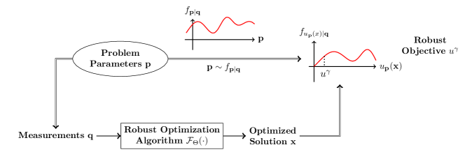
Figure 1: The robust optimization problem for maximizing a $\gamma$-percentile outage utility based on a measurement of the problem parameters.

This paper aims to solve the the robust optimization problem (3) above based on the measurements $\mathbf{q}$ of the unknown problem parameters $\mathbf{p}$ by producing an optimized variable $\mathbf{x}$ that maximizes the robust objective under the outage constraint.

In this end, this paper proposes to utilize a deep learning approach to map the measurement of the optimization problem parameters to a robust optimized solution. The deep neural network is chosen for its computation capacity and representation ability. Using a neural network, the optimization algorithm can be represented as:

$$\mathbf{x}={\mathcal{F}}_{\Theta}(\mathbf{q})$$ (4)

where $\Theta$ is the collection of the neural network model parameters and hyper-parameters. The optimization problem $\mathcal{P}$ then translates to finding a set of high-quality neural network parameters $\Theta$. The overall optimization process is shown in Fig. 1.

III Robust Optimization in Wireless Communications and Networking

We now present two applications of the above general robust optimization framework in wireless network utility maximization: the robust power loading problem for multiuser MIMO transmissions and the robust power control problem for D2D networks. Wireless network utility optimization problems naturally fit into the robust optimization framework, since the wireless channels (i.e. the problem parameters $\mathbf{p}$) are difficult to measure accurately, and the channel estimation process always produces measurement uncertainties.

III-A Robust Beamforming for Minimum Rate Maximization in Multiuser MIMO Downlink

Consider a MIMO transmission scenario with one base station equipped with $M$ antennas serving $K$ single-antenna users. The base station serves all $K$ users through multiuser MIMO downlink transmission in the same time-frequency resource block. We use $\mathbf{H}=[\mathbf{h}_{1},\dots,\mathbf{h}_{k},\dots,\mathbf{h}_{K}]\in\mathbb{C}^{M\times K}$ to denote the channel matrix, with its $k$-th column $\mathbf{h}_{k}\in\mathbb{C}^{M\times 1}$ denoting the channels from the base station antennas to the $k$-th user. In practical wireless communication scenarios, $\mathbf{H}$ is often not known perfectly. The goal is to design robust downlink beamforming vectors against the uncertainties in $\mathbf{H}$. A diagram illustrating the downlink multiuser MIMO channel is shown in Fig. 2.

In a dense urban environment, there are often no line-of-sight (LoS) paths from the base station to the users, and the wireless channels in the multiuser MIMO networks can be modeled as a Rayleigh fading channel [58]. To estimate the channel, pilot signals need to be used. For time-division duplex (TDD) systems, uplink pilots from the users to the base station can be used to estimate the uplink channel. Then, based on the uplink-downlink reciprocity, the downlink channel can be inferred. For frequency-division duplex (FDD) systems, downlink pilots from the base station to the users need to be used. In this case, each user estimates its own channel, then feeds back a quantized version of the channels to the base station in order to enable the base station to design the downlink beamformers based on the estimated channels from all the users.

Figure 2: Multiuser MIMO Downlink Channel

In either case, the accuracy of the estimated channels $\hat{\mathbf{H}}$ depends on the pilot length, the background noise level, and in the FDD case is also a function of feedback rate. A common way to model the channel estimation error is to assume that for the wireless channel from the $j$-th base station antenna to the $k$-th user, the relationship between the real channel coefficient $h_{kj}$ and the estimated channel coefficient $\hat{h}_{kj}$ can be modeled as the following:

$$h_{kj}=\hat{h}_{kj}+e_{kj},\;e_{kj}\sim\mathcal{CN}(0,\sigma_{e}^{2})\quad\forall j,k$$ (5)

where the estimation error $e_{kj}$ is independent and identically distributed (i.i.d.) across all the channels.

The robust beamforming problem for the multiuser MIMO system is that of designing the beamformers at the base station, along with the power loading for each beamformer, in order to achieve a robust objective. In this paper, we treat the optimization objective of maximizing the minimum rate in order to provide fairness across all the users. Although ideally, one could conceivably design both the beamformers and the power loadings jointly to account for the channel uncertainty, such an approach would have been too challenging due to its analytic complexity. In the existing literature, only the robust optimization for the simpler objective of power minimization has been shown to be possible to solve analytically over both the beamformers and the power allocation variables [49, 50, 51]. In contrast, this paper adopts a different approach: we fix the beamformers and assume that the design of the beamformers can be done based on $\hat{\mathbf{H}}$ only, then rely on the subsequent power allocation to ensure robustness. This design approach can be an effective one due to that it significantly simplifies the overall design process, while still achieving competitive robust performances as shown in [52, 53].

More specifically, based on the estimated channels $\hat{\mathbf{H}}$, the base station can apply any one of the well-established beamforming techniques, such as zero-forcing (ZF) or regularized zero-forcing (RZF) [59], to design a fixed set of precoders $\mathbf{B}\in\mathbb{C}^{M\times K}$ for downlink transmission. We use the notation $\mathbf{B}=[\mathbf{b}_{1},\dots,\mathbf{b}_{k},\dots,\mathbf{b}_{K}]$, with the $k$-th column $\mathbf{b}_{k}\in\mathbb{C}^{M\times 1}$ with unit norm $\|\mathbf{b}_{k}\|_{2}=1$ being the beamformer from the base station to transmit information to the $k$-th user.

The robust optimization variables are now the set of power loading variables $\mathbf{x}=\{x_{k}\}_{k\in[1\dots K]}$, where $x_{k}\in[0,1]$ denotes the proportion of total power the base station should allocate for transmitting to the $k$-th user for optimizing a network-wide utility $u_{\mathbf{p}}(x)$. In this paper, we use the minimum rate across all the users as the utility. Note that for given $\mathbf{x}$, the achievable rate for the $k$-th user is computed as

$$r_{k}=w\log\left(1+\frac{P|\mathbf{h}_{k}^{H}\mathbf{b}_{k}|^{2}x_{k}}{P\sum_{j\neq k}|\mathbf{h}_{k}^{H}\mathbf{b}_{j}|^{2}x_{j}+\sigma^{2}}\right),$$ (6)

where $P$ denotes the total power constraint, $w$ denotes the bandwidth, $\sigma^{2}$ denotes the background noise level, and $(\cdot)^{H}$ denotes Hermitian transpose.

For any $\mathbf{x}$, the statistical channel uncertainties induce a distribution on the achievable rates of each user, and consequentially, a distribution on $r_{\min}$, the minimum rate among all the users. We can compute the percentile value $r_{\min}^{\gamma}$ of the distribution for $r_{\min}$ as the maximum value for which:

$$\mathrm{Pr}[r_{\min}<r_{\min}^{\gamma}|\hat{\mathbf{H}}]\leq\gamma\%.$$ (7)

With these notations established, the multiuser MIMO robust beamforming problem is now readily formulated as an instance of the robust optimization problem $\mathcal{P}$ as in Section II-B, with the following correspondence:

$$\mathbf{p}\leftarrow \>\mathbf{H}$$

$$\mathbf{q}\leftarrow \>\hat{\mathbf{H}}$$

$$u_{\mathbf{p}}({\mathbf{x}})\leftarrow \>r_{\min}$$

$$u^{\gamma}\leftarrow \>r_{\min}^{\gamma}$$

The robust power loading problem for maximizing the minimum-rate in a multiuser MIMO downlink, which we denote by $\mathcal{P}_{\text{MIMO}}$, is then formulated as follows:

$$\underset{\mathbf{x}}{\text{maximize}}\quad r_{\min}^{\gamma}$$ (8a)

subject to $$\mathrm{Pr}[r_{\min}<r_{\min}^{\gamma}|\hat{\mathbf{H}}]\leq\gamma\%$$ (8b)

$$r_{\min}\leq r_{k},\;\forall k$$ (8c)

$$\sum_{k=1}^{K}x_{k}\leq 1,\quad x_{k}\geq 0,\;\forall k$$ (8d)

$$\text{and }(\ref{equ:MIMO_uncertainty}),(\ref{equ:MIMORate}).$$

III-B Robust Power Control for Minimum Rate Maximization in D2D Wireless Networks

Figure 3: D2D Interfering Network

Consider a wireless ad-hoc network with $N$ independent D2D links with full frequency reuse in a two-dimensional region as illustrated in Fig. 3. The goal is to find a set of power setting at each transmitter so as to be able to mutually accommodate the simultaneous transmissions for all links. In this application, we again use the minimum rate across all the users as the network utility function, in order to ensure fairness. This is a challenging task, because due to the aggressive frequency reuse in the shared medium, the aggregate interference from the neighboring links pose as significant impairments to each of the transmission pairs.

In the setting considered in this paper, we assume that the transmitters and the receivers are equipped with multiple antennas, further the links operate in the millimeter wave (mmWave) frequency and there is a dominant LoS path between each transmitter and receiver pair. Moreover, we assume that in the network deployment phase, a beam alignment procedure has taken place between each transmitter-receiver pair, so that all the direct channels can benefit from a substantial array gain. Then, an additional power optimization step across all the users is performed to ensure that the aggregated interference is under control for each transmission pair. Here, we focus on the power optimization step.

To formulate and to solve a power optimization problem across $N$ transmitting and receiving nodes using traditional mathematical programming technique, one would need to estimate not only all the direct channels, but also all the interfering channels between every transmitter and every receiver. In a network of $N$ transmission pairs, one would need a dedicated pilot phase of duration at least $O(N^{2})$ in order to estimate all of the $N^{2}$ channel coefficients. This is often infeasible.

In this part of the paper, we explore the possibility of performing power control purely based on the geographic location information of all the transmitters and the receivers. The geographic location information already provides the pathloss component of the overall channel. The idea is to formulate a robust optimization problem, so that a reasonable minimum rate across all the users can still be achieved with high probability, even if the power control is based only on the pathloss information.

Another benefit of utilizing geographic location information is that such information can also be readily used for computing the beamformers at the transmitters and the receivers based on the angles of arrival and departure of the intended signal transmission to align the beams of the transmitter and the receiver towards each other in the initial deployment phase.

In the ensuing channel model, we use $\hat{\mathbf{G}}^{\mathrm{PL}}$ to denote the path-losses of all the channels, including the beamforming gains at both the transmitters and the receivers. In addition, we assume a log-normal shadowing component and a fast-fading component that contribute towards the uncertainties in the channel model. Specifically, we assume a log-normal distribution for the shadowing $\mathbf{G}^{\mathrm{S}}$, and a circularly symmetric complex Gaussian distribution for the fast fading coefficients that lead to a fast fading component $\mathbf{G}^{\mathrm{F}}$. Then, the overall channel $\mathbf{G}$ has its $(i,j)$-th component distributed as:

$$g_{ij}= \>\hat{g}^{\mathrm{PL}}_{ij}g^{\mathrm{S}}_{ij}g^{\mathrm{F}}_{ij}$$ (9)

with the log-normal shadowing component as

$$g^{\mathrm{S}}_{ij}=10^{\frac{g^{\mathrm{S}\text{dB}}_{ij}}{10}},\qquad g^{\mathrm{S}\text{dB}}_{ij}\sim\mathcal{N}(0,\sigma_{S}^{2}),\qquad\forall i,j$$

and the Rayleigh fading component as

$$g^{\mathrm{F}}_{ij}\sim\chi^{2}(2),\qquad\forall i,j$$

where $\sigma_{S}$ is the standard deviation of the shadowing in the dB scale, while the standard deviation of the circularly symmetric complex Gaussian distribution for the fast fading coefficients is assumed to be 1. Here, $\chi^{2}(2)$ denotes the chi-squared distribution with 2 degrees of freedom.

The robust optimization variables are the set of power control variables $\mathbf{x}=\{x_{i}\}_{i\in[1\dots N]}$, where $x_{i}\in[0,1]$ denotes the proportion of total $p_{i}$ the $i$-th transmitter should transmit. Given $\mathbf{x}$, the achievable rate for the $i$-th link is computed as

$$r_{i}=w\log\left(1+\frac{g_{ii}p_{i}x_{i}}{\sum_{j\neq i}g_{ij}p_{j}x_{j}+\sigma^{2}}\right),$$ (10)

where $w$ is the bandwidth, $p_{i}$ is the power budget of link $i$, and $\sigma^{2}$ is the background noise power.

Under a fixed power allocation $\mathbf{x}$, the statistical variations of the channel result in statistical variations in the achievable rate of each link. As a result, the minimum rate among all the links, i.e.,

$$r_{\min}=\min_{i=1,\cdots,N}r_{i}$$ (11)

also follows a distribution induced by the channel uncertainties. As in Section II-B, we adopt the $\gamma$-th percentile value of the minimum rate distribution, $r_{\min}^{\gamma}$, as the objective value, i.e., $r_{\min}^{\gamma}$ is the largest value for which

$$\mathrm{Pr}[r_{\min}<r_{\min}^{\gamma}|\hat{\mathbf{G}}^{\mathrm{PL}}]\leq\gamma\%.$$ (12)

This corresponds to the notion of outage capacity. Note that here we consider the outage in minimum rate over the entire network instead of over individual links. Instead of computing the outage rate of each link, as in the earlier work [47, 48] and the conference version of this paper [1], the percentile rate is taken after the network utility is computed.

The robust optimization problem for the D2D network can now be formulated as follows. We assume that a central controller has access to only the path-loss components and the beamforming gains of all the channels, and seeks to find a set of robust power allocations that work well over different realizations of the shadowing and fast fading components. This D2D wireless network power control problem is therefore one instance of the robust optimization problem $\mathcal{P}$ in Section II-B. We have the following correspondence:

$$\mathbf{p}\leftarrow \>\mathbf{G}$$

$$\mathbf{q}\leftarrow \>\hat{\mathbf{G}}^{\mathrm{PL}}$$

$$u_{\mathbf{p}}(\mathbf{x})\leftarrow \>r_{\min}$$

$$u^{\gamma}\leftarrow \>r_{\min}^{\gamma}$$

The robust power control for minimum-rate maximization problem in D2D wireless networks, which we denote by $\mathcal{P}_{\text{D2D}}$, is then

$$\underset{\mathbf{x}}{\text{maximize}}\quad r_{\min}^{\gamma}$$ (13a)

subject to $$\mathrm{Pr}[r_{\min}<r_{\min}^{\gamma}|\hat{\mathbf{G}}^{\mathrm{PL}}]\leq\gamma\%$$ (13b)

$$r_{\min}\leq r_{i},\;\forall i$$ (13c)

$$0\leq x_{i}\leq 1,\;\forall i$$ (13d)

$$\text{and }(\ref{equ:D2D_uncertainty}),(\ref{equ:D2DRate}).$$

IV Uncertainty Injection: A Deep Learning Training Scheme for Robust Optimization

This section presents a novel uncertainty injection scheme for training deep learning models for solving robust optimization problems. The goal is to train a model to produce solutions that maximize a utility subject to an outage constraint. The proposed training scheme is applicable to a wide variety of problems and different neural network architectures, requiring only the assumption that the utility can be easily evaluated under different problem parameters.

IV-A Sample-based Uncertainty Distribution Characterization

Natural phenomena often induce uncertainties that are difficult to characterize accurately. Their distributions can have unbounded support, and are often not easily expressed by tractable mathematical expressions. Traditional robust optimization algorithms rely on building mathematical models for the distributions of the uncertainties, then performing optimization based on these models. Imposing mathematical models has two major drawbacks: the models may not fully characterize the true uncertainty distributions; further the subsequent optimizations are often not analytically tractable, may require extra simplifications, and may result in significant computational complexities for obtaining the final solution.

In this paper, we advocate characterizing parameter uncertainties via sampling. Samples of the uncertainty can be straightforward to generate for many realistic applications. With sufficient number of samples, we can estimate the statistical objective numerically, thus eliminating the need for mathematical models and the associated analysis. Sampling has been widely used in many machine learning algorithms, such as stochastic gradient descent [60], evolutionary algorithm [61], variational inference [5], and so on. In this paper, we use a sampling strategy to develop robust optimization algorithms that are more flexible and more computationally efficient than traditional mathematical optimization algorithms.

IV-B Uncertainty Injection Scheme

We propose an approach of training a neural network to solve the robust optimization problem $\mathcal{P}$. The neural network takes measurements of the problem parameters as input, i.e., $\mathbf{q}$, and computes a robust solution $\mathbf{x}$. The mapping from $\mathbf{q}$ to $\mathbf{x}$ can be modeled by any neural network structure. The key for our training scheme is the injection of uncertainty realizations of the problem parameters into the training process, after $\mathbf{x}$ is computed.

Specifically, during the training stage, after the neural network computes the solutions $\mathbf{x}$ based on $\mathbf{q}$, we inject a large number of $L$ problem parameters realizations $\{\mathbf{p}_{1},\mathbf{p}_{2},\mathbf{p}_{3},\dots,\mathbf{p}_{L}\}$, sampled from $f_{\mathbf{p}|\mathbf{q}}(\mathbf{p}|\mathbf{q})$, at the output layer by computing the objective values of the optimization problem for each of these samples of problem parameters, i.e., $u_{\mathbf{p}_{1}}(\mathbf{x}),u_{\mathbf{p}_{2}}(\mathbf{x}),\dots,u_{\mathbf{p}_{L}}(\mathbf{x})$. From these set of objective values, we can obtain $\hat{u}^{\gamma}$, an empirical estimate of $u^{\gamma}$, by ranking the $L$ objective values and take the ${(L\gamma)}$-th lowest value (with linear interpolation if $L\gamma$ is not an integer). Based on the gradients derived from $\hat{u}^{\gamma}$, we update the neural network weights $\Theta$ to improve the robust objective performance in an unsupervised learning fashion. The idea is that during testing, the neural network can compute $\mathbf{x}$ based only on $\mathbf{q}$, but can nevertheless achieve statistical robustness against the unseen uncertainties in $\mathbf{p}$.

The overall neural network structure is shown in Fig. 4. During training, the computation flows all the way towards the end for computing $\hat{u}^{\gamma}$; while during testing or for applications, the computation stops at the output layer for the optimization variables $\mathbf{x}$.

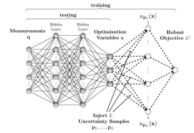
Figure 4: Uncertainty injection scheme for training a neural network for robust optimization

We emphasize that the proposed method of training with uncertainty realizations injection is fundamentally different from the idea of data augmentation, in which various transformations or noises are applied to the training data before feeding to the model [4, 62]. Our method is also fundamentally different from existing literature on noise injection for robust deep learning, in which noises are injected to the inputs [25, 26, 27, 28, 29], the neural network parameters [30], the activation functions [31, 32], and the gradients [33, 34], as already mentioned earlier. In contrast, the proposed strategy injects uncertainties after the neural network output layer, and updates the neural network model in an unsupervised fashion, based on an objective which is a stochastic function of the input (i.e., optimizing the $\gamma$-th percentile of $u_{\mathbf{p}}(\mathbf{x})$ when the neural network input provided is $\mathbf{q}$). This is a sensible strategy in the robust optimization setting because the task at hand is an explicitly formulated mathematical optimization problem, and the output of the neural network is a solution to this problem, for which we can readily evaluate its robustness under the uncertain problem parameters. The proposed strategy uses injected uncertainty realizations to compute an robust objective, then trains the neural network to maximize this objective. This training scheme allows the neural network to implicitly learn the underlying uncertainty distribution for achieving robustness in its solutions, which is impossible to do under data augmentation or existing noise injection methods in the literature.

IV-C Gradient Computation for Back-Propagation

We now elaborate on the mathematical details of the gradient back-propagation under the uncertainty injection training scheme. With $\mathbf{x}$ computed by a usual neural network, the learned $\mathbf{x}$ is a differentiable function of the neural network parameters $\Theta$. In the meanwhile, the objective function $u_{\mathbf{p}}(\mathbf{x})$ is assumed to be differentiable (almost everywhere) over $\mathbf{x}$ for fixed problem parameters $\mathbf{p}$. Lastly, the sample-based empirical percentile value $\hat{u}^{\gamma}$, even with possible linear interpolation between two points, is differentiable with respect to the sampled objective values $\{u_{\mathbf{p}_{1}}(\mathbf{x}),u_{\mathbf{p}_{2}}(\mathbf{x}),\dots,u_{\mathbf{p}_{L}}(\mathbf{x})\}$ in a local neighborhood. This is because the percentile value does not depend on most of the sampled objective values, except one or two closest to the target percentile. When $L$ is finite, the rankings of the sampled objective values closest to the target percentile do not change in the local neighborhood, so differentiability can be ensured locally almost surely.

We emphasize that the uncertainty injection scheme is not restricted to the percentile function as the notion of robustness. As long as robustness is defined by a function whose sample-based approximation is differentiable over the samples, we can train a deep learning model for this robustness objective using the uncertainty injection scheme.

Taken together, we have that the empirical robust objective $\hat{u}^{\gamma}$ is a differentiable function over the neural network model parameters $\Theta$. Therefore, the neural network can be optimized with the stochastic gradient descent method when being trained with the uncertainty injection scheme.

To compute the gradients, let $\mathbf{p}_{i}$ be the uncertainty realization (among the set of $L$ injected uncertainty samples) whose corresponding objective $u_{\mathbf{p}_{i}}(\mathbf{x})$ is the empirical $\gamma$-th percentile value of the set of sample objectives, i.e., $\hat{u}^{\gamma}$. The gradient of $\hat{u}^{\gamma}$ with respect to the neural network parameters $\Theta$ can be obtained by the chain-rule of differentiation:

$$\frac{\partial\hat{u}^{\gamma}}{\partial\Theta}=\frac{\partial\hat{u}^{\gamma}}{\partial u_{\mathbf{p}_{i}}(\mathbf{x})}\frac{\partial u_{\mathbf{p}_{i}}(\mathbf{x})}{\partial\mathbf{x}}\frac{\partial\mathbf{x}}{\partial\Theta}=\frac{\partial u_{\mathbf{p}_{i}}(\mathbf{x})}{\partial\mathbf{x}}\frac{\partial\mathbf{x}}{\partial\Theta},$$ (14)

where the term $\frac{\partial\hat{u}^{\gamma}}{\partial u_{\mathbf{p}_{i}}(\mathbf{x})}$ is 1; the term $\frac{\partial u_{\mathbf{p}_{i}}(\mathbf{x})}{\partial\mathbf{x}}$ can be computed based on the uncertainty realization $\mathbf{p}_{i}$; and lastly, the term $\frac{\partial\mathbf{x}}{\partial\Theta}$ depends on the number of activation layers and the values of $\Theta$ themselves in the neural network. In other words, the gradient of $\gamma$-th percentile robust objective is just the gradient of the objective corresponding of the $\gamma$-th percentile realization $\mathbf{p_{i}}$.

While the exact expressions for these gradients depend on the neural network structure and the objective function $u_{\mathbf{p}}(\mathbf{x})$, all of these differentiations are readily computed by popular deep learning frameworks such as Pytorch [63] or Tensorflow [64]. Therefore, the uncertainty injection scheme adds very little complexity to the training of deep neural networks, and no extra complexity at testing.

IV-D Sample-Based Gradient Estimator

The previous section establishes the gradient computation for optimizing the robust objective and shows that the proposed robust optimization process can be easily implemented in the usual deep learning computation frameworks. We now show that the sample-based gradient in (14) is an asymptotically unbiased estimator of the true desired gradient.

Let $u^{\gamma}$ be the true $\gamma$-th percentile of $u^{\mathbf{p}}(\mathbf{x})$ under $\mathbf{p}\sim f_{\mathbf{p}|\mathbf{q}}(\mathbf{p}|\mathbf{q})$, i.e., the population statistic. Let $\hat{u}^{\gamma}$ be the $\gamma$-th percentile of the samples $\{u_{\mathbf{p}_{1}}(\mathbf{x}),u_{\mathbf{p}_{2}}(\mathbf{x}),\dots\,u_{\mathbf{p}_{L}}(\mathbf{x})\}$, i.e. the sample statistic. Let $\frac{\partial u^{\gamma}}{\partial\Theta}$ be the true gradient for updating the neural network parameters assuming that the gradient exists, (or a supergradient if the gradient does not exist).

We now examine the sample-based gradient in (14) under the expectation. As described in Section IV-B and Section IV-C, the sample statistic $\hat{u}^{\gamma}$ is obtained by sorting the sample objective values then finding the index corresponding to the percentile in the samples, (i.e., with sample size being $L$, we find the value ranked the $(L\gamma)$-th lowest, with linear interpolation if necessary). As shown in [65, 66], under fairly general conditions, this sample statistic is an asymptotically unbiased estimator to the true population statistic $u^{\gamma}$. Therefore, we have:

$$\lim_{L\to\infty}\mathbb{E}[\hat{u}^{\gamma}]=u^{\gamma}.$$ (15)

It can be seen that the expectation of the gradient (14), in the asymptotic limit of large sample size, is just $\frac{\partial u^{\gamma}}{\partial\Theta}$:

$$\lim_{L\to\infty}\mathbb{E}\left[\frac{\partial\hat{u}^{\gamma}}{\partial\Theta}\right]= \>\frac{\partial\lim_{L\to\infty}\mathbb{E}[\hat{u}^{\gamma}]}{\partial\Theta}$$ (16)

$$= \>\frac{\partial u^{\gamma}}{\partial\Theta}$$ (17)

where (17) follows from the linearity of both the limit and the expectation operators, and the fact that the interchange of the limit, the expectation and the derivatives is allowed under certain regularity conditions. Assuming that such regularity conditions hold for the distribution $u_{\mathbf{p}}(\mathbf{x})$, we have that in the uncertainty injection scheme, the gradients used in updating the neural network weights are asymptotically unbiased estimators of the true gradients, which is a desirable property for the convergence of the training of deep learning models. We note that this analysis resembles the proof that the gradient estimator of the stochastic gradient descent (SGD) algorithm [60] is unbiased.

V Applications of Uncertainty Injection in Wireless Communications

In this section, we describe the application of the uncertainty injection training scheme for solving robust optimization in wireless communication problems as described in Section III. Further, we describe the benchmarks that the proposed training method would be compared with in the numerical evaluation.

V-A Neural Network Architecture and Uncertainty Injection

For the two applications as described in Section III-A and Section III-B, given the inputs as the estimated MIMO wireless channels or the path-loss components in a D2D wireless network, the neural network computes robust maximum minimum-rate solutions for power loading at the base station or power control among D2D links.

Robustness is achieved using the uncertainty injection training scheme, in which a large set of wireless channel realizations are sampled and injected at the output of the neural network. A set of minimum rates can then be computed, with one minimum rate for each of the channel realization. This set of rates provides an empirical distribution of the minimum rate over the uncertain channels. We then take the $\gamma$-th percentile value of this set of rates $\hat{r}_{\min}^{\gamma}$ as the empirical estimation for $r_{\min}^{\gamma}$. Through computing gradient and performing gradient ascent on $\hat{r}_{\min}^{\gamma}$, the neural network is trained towards the direction of improving the robust minimum rate.

To explore the full potential of the training scheme with deep learning, we design the neural network based on the most general architecture: the fully connected neural networks. Following an input layer which takes channel measurement values $\mathbf{q}$, we adopt fully connected hidden layers each with ReLu non-linearity activations. In the output layer that computes the solutions for optimization variables $\mathbf{x}$, proper non-linear activations are used to account for the constraints on the variable $\mathbf{x}$.

During the training for each single input, we sample and inject $L=1000$ uncertainty realizations. Correspondingly, at any point of training, following each neural network forward path, we compute 1000 $u_{\mathbf{p}}(\mathbf{x})$ objective values based on the $\mathbf{x}$ computed by the neural network. The $\gamma$-th percentile objective among these 1000 $u_{\mathbf{p}}(\mathbf{x})$ objective values is then selected for computing the gradient and performing gradient ascent on the neural network parameters $\Theta$.

V-B Robust Objective vs. Nominal Objective

We show two types of objectives in the numerical simulations: the robust objective and the nominal objective. The robust objective is as specified by the robust optimization formulation $\mathcal{P}$, i.e., the $\gamma$ percentile value of the objective distribution achieved by the solution $\mathbf{x}$, as induced by the uncertainty distribution.

On the other hand, the nominal objective is the objective value achieved by the solution $\mathbf{x}$, under the measured (or estimated) input values as if they are the true channel parameter values. Under our notation, the nominal objective is denoted as $u_{\mathbf{q}}(\mathbf{x})$.

We show the results for the nominal objective, because it is the objective that deterministic optimization algorithms (i.e. the non-robust optimization algorithms) would optimize, assuming that the measured or estimated problem parameters are entirely accurate. The relative performances of all the methods in terms of their nominal objective and the robust objective reveal the effectiveness of actively accounting for the channel uncertainties during optimization.

V-C Deep Learning without Uncertainty Injection

To fully illustrate the benefits of the proposed the training scheme, we include a benchmark method where an identical neural network is trained with the same dataset and hyper-parameters, but without uncertainty injection. Specifically, we train the neural network with the same unsupervised learning procedure, except that we do not implement any uncertainty injection. Instead, during training the gradient is derived from the nominal objective $u_{\mathbf{q}}(\mathbf{x})$, computed directly based on the measured or estimated channel parameters $\mathbf{q}$.

We note that to the best of the authors knowledge, there are no efficient analytic mathematical optimization methods that can account for channel uncertainties in these problem settings.

VI Experimental Validation

This section provides numerical results for the proposed uncertainty injection scheme on two wireless network applications, namely, the robust power loading problem for the multiuser MIMO downlink, and the robust power control problem for D2D wireless networks.

VI-A Multiuser MIMO Downlink Environment

Consider a base station equipped with $M=4$ antennas and serving $K=4$ users. We assume the i.i.d. Rayleigh fading model for the MIMO channel $\mathbf{H}$, with each channel entry following a circularly symmetric complex Gaussian distribution $h_{kj}\sim\mathcal{CN}(0,1),\>\forall k,j$. We assume that the channel estimation error $e_{kj}$ as in (5) has a variance of $\sigma_{e}^{2}=0.075$. During data transmission, we assume the total power constraint $P$ of 1W over a bandwidth of 10MHz, and an effective background noise level of -75dBm/Hz (e.g., after accounting for pathloss and out-of-cell interference).

Prior to the power loading optimization, based on the estimated channels $\hat{\mathbf{H}}$ using minimum mean-square estimation (MMSE) [67], we utilize the RZF beamformers, which have a better performance than the ZF beamformers. Specifically, we compute the unnormalized RZF beamformers as follows:

$$\mathbf{B}^{\prime}=\hat{\mathbf{H}}(\hat{\mathbf{H}}^{H}\hat{\mathbf{H}}+\alpha\mathbf{I})^{-1}$$ (18)

To choose an appropriate value for $\alpha$, we make the following observation (which is verified by numerical simulations): as $\alpha$ approaches zero, the beamformers become more aggressive on nulling the interference, but also become more sensitive with respect to channel uncertainty. As a result, the nominal objective (as defined in Section V-B) increases while the robust objective degrades. To achieve a reasonable trade-off on the regularization factor, we select the value of $\alpha$ that results in the highest medium $r_{\min}$ under the channel uncertainty distribution (assuming equal power allocation across the users for simplicity). This leads to a value of $\alpha=0.2$ in our setting.

We then normalize the beamformers across each column of $\mathbf{B}^{\prime}$, i.e., the beamformers for each user, to unit norm, to obtain the normalized beamformers $\mathbf{B}$.

For the inputs to the neural network, we compute the effective channels $\hat{\mathbf{H}}_{\text{eff}}$ based on $\hat{\mathbf{H}}$ and $\mathbf{B}$ as:

$$\hat{\mathbf{H}}_{\text{eff}}=\hat{\mathbf{H}}^{H}\mathbf{B}$$ (19)

and flatten the resultant matrix into a length-$(K\times K)$ vector. We note that this information is the measurement of the channel, i.e., playing the role of $\mathbf{q}$ in the robust optimization problem $\mathcal{P}$ as in Section II-B.

Provided with this input, the fully-connected neural network then computes the output $\mathbf{x}\in[0,1]^{K}$ as the power loading solution. We use the softmax activation at the final output layer to enforce the power constraint $\sum_{i=1}^{K}x_{i}\leq 1$.

Lastly, to train the neural network with uncertainty injection scheme for robust minimum-rate optimization, we randomly generate 1000 channel realizations of $\mathbf{H}$ according to (5) and inject them into the neural network training flow. With a specific solution $\mathbf{x}$ computed by the neural network, we compute then take the minimum of the $K$ user rates achieved for each of the 1000 channel realizations. We then take the $\gamma$-th percentile of those 1000 minimum rates to obtain the empirical estimation $\hat{u}^{\gamma}$. The gradient to update the neural network weights is computed based on the channel realization corresponding to $\hat{u}^{\gamma}$.

During training, we use a minibatch size of 1000 distinct MIMO networks, with each training epoch including 50 minibatches. We train for a total of 500 epochs, with early stopping based on validation at the end of each epoch. We note that instead of having a fixed training set, we continuously generate new MIMO network wireless channels and their estimations, which is easy to do because of the readily available Rayleigh fading channel model.

TABLE I: Multiuser MIMO Downlink 5-Percentile Robust Minimum-Rate Performance

Methods	Nominal Minimum Rate	Robust Minimum Rate
Geometric Programming	40.18Mbps	5.41Mbps
Deep Learning without Uncertainty Injection	39.51Mbps	6.52Mbps
Deep Learning with Uncertainty Injection	37.40Mbps	8.03Mbps
Uniform Power	29.70Mbps	5.88Mbps

VI-B Multiuser MIMO Downlink Results

We adopt a structure for the neural network with 4 fully-connected layers, each with 200 hidden neurons and the ReLU non-linearity, except for the output layer with the softmax non-linearity to ensure that $\sum x_{i}=1$. (In the low-interference regime after RZF, the optimized $\mathbf{x}$ is likely to be a one that uses up all the total power, i.e., (8d) is satisfied with equality.) This same structure is also use in the deep learning without uncertainty injection benchmark as described in Section V-C.

We also compare with a geometric programming benchmark, which finds the global optimal solution for the minimum-rate maximization problem by representing the inverse of the signal-to-inference-and-noise ratio (SINR) terms as posynomials [68]. Note that the formulation required by geometric programming cannot incorporate channel uncertainties, because the statistical robustness of the objective cannot be expressed by posynomials.

In the simulations, we set $\gamma=5$, i.e., we use the robust minimum rate at the 5th-percentile across the distribution induced by the channel uncertainties as the robust objective. We evaluate the robust minimum rate and the nominal minimum rate performances over 2000 testing layouts. For evaluation of the robust objective, we also use 1000 randomly sampled channel realizations on each of the 2000 testing layouts to empirically estimate the 5th-percentile value of the minimum rates. The results are presented in Table I. Furthermore, the cumulative distribution function (CDF) of these robust 5th-percentile minimum-rates over all 2000 testing layouts are shown in Fig. 5.

As the numerical results show, the neural network trained with the uncertainty injection scheme achieves 23% improvement on the robust minimum rate over the same neural network trained without uncertainty injection. This shows that the uncertainty injection scheme indeed encourages the deep learning model to learn and to produce solutions that are significantly more robust against the channel uncertainties than the state-of-the-art algorithms.

Interestingly, the performance improvement over geometric programming is even larger, at 48% for the robust 5th-percentile minimum-rate. This is because the classical mathematical programming techniques exploit the particular channel realization to the fullest extent in order to maximize the minimum-rate objective, as shown in the nominal minimum rate result, but it does not account for robustness across the channel uncertainties at all. Even training a neural network to approximate the classical mathematical programming without uncertainty injection would already achieve some robustness, as shown in Fig. 5. Significantly better robustness is achieved with training a deep neural network with uncertainty injection.

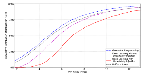
Figure 5: Cumulative distribution of 5th-percentile robust minimum-rates in MIMO wireless networks over 2000 test channel layouts.

VI-C D2D Wireless Network Environment

For the D2D wireless network, we consider a number of D2D links randomly deployed within a confined region, with the transceiver distances following uniform distributions. We impose a minimum of 5-meter distance between any transmitter and any receiver that do not belong to the same link. For the path-loss, we follow the short-range outdoor model ITU-1411, with 5MHz bandwidth at the carrier frequency of 25GHz (the mmWave range).

Every transmitter and receiver is equipped with a linear antenna array with $M=8$ antennas. We use a beamforming pattern corresponding to a uniform linear array directly aimed between the transmitter and the receiver. The beamforming gains are approximated as follows: 9dB gain for the direct links (as the transmitter and receiver pair can align with each other precisely), 6dB gain at the main lobe direction with an angle from $-10$ to $+10$ degrees, and $-9$dB gain at the side lobe directions. In Fig. 6, the corresponding beamforming gain pattern and its approximation are plotted for $M=8$. At each transmitter, we assume a maximum transmit power of 30dBm. We also assume a background noise level of $-169$dBm/Hz.

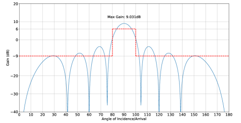
Figure 6: D2D beamforming pattern at the transmitters and the receivers, and its approximation used in simulations.

We incorporate the following channel uncertainty models for each direct and interfering links:

• Shadowing with log-normal distribution with 8dB standard deviation;

• Rayleigh fading with i.i.d. circularly symmetric complex Gaussian distribution with unit variance.

Furthermore, to illustrate that the training process can be applied to different scenarios, we test the robust performances in three different settings with 1000 wireless networks layouts under each setting, as in Table II. For each layout, we sample 1000 channel realizations during testing to obtain an empirical approximation of the robust minimum rate across the entire network.

TABLE II: D2D Wireless Environment

Setting	Number of Links ($N$)	Region Area $(m^{2})$	Direct-Link Distance Distribution
A	10	$150\times 150$	5m$\sim$15m
B	10	$200\times 200$	20m$\sim$30m
C	15	$300\times 300$	10m$\sim$30m

VI-D D2D Wireless Networks Results

We adopt a neural network structure with 5 fully-connected layers, each with 6$N^{2}$ hidden neurons and the ReLU non-linearity, except for the output layer, which produces $\mathbf{x}$ with $N$ output units and has a sigmoid non-linearity (to ensure that the power control solution for the $N$ links has a range of $[0,1]^{N}$). This same structure is also used for the benchmark of deep learning without uncertainty injection as described in Section V-C.

Because of the path-loss, the direct and the interfering links are often of different orders of magnitudes, making it difficult to obtain meaningful updates at the beginning of training. To make training effective, we adopt input normalization on the input path-loss values (for both training and testing), where each of the $N^{2}$ inputs of the path-loss values are normalized independently based on the statistics computed from the training set.

For the D2D network simulations, we set $\gamma=10$, i.e., we use the minimum rate at the 10th percentile across the distribution induced by the channel uncertainties as the robust objective. We present test results on the robust minimum-rate obtained by the neural network based only on the path-loss and the beamforming gain values as the inputs. Similar to Section VI-B, we include two benchmarks for illustrating the importance of robust optimization: deep learning without uncertainty injection, and the geometric programming (which can provide globally optimal solutions if the channel uncertainties are not considered). Results are shown in Table III. Fig. 7 presents CDF curves of the robust minimum-rates achieved by all methods over 1000 testing wireless networks, generated under test setting B in Table II.

TABLE III: D2D Wireless Networks Robust Minimum-Rate Performance

Methods	Setting A		Setting B		Setting C
	Nominal	Robust	Nominal	Robust	Nominal	Robust
Geometric Programming	46.84Mbps	2.72Mbps	37.05Mbps	0.86Mbps	40.36Mbps	0.85Mbps
Deep Learning without Uncertainty Injection	44.86Mbps	3.78Mbps	35.41Mbps	1.21Mbps	37.56Mbps	1.37Mbps
Deep Learning with Uncertainty Injection	43.18Mbps	4.03Mbps	33.81Mbps	1.31Mbps	35.70Mbps	1.41Mbps
Full Power	37.43Mbps	3.29Mbps	28.61Mbps	1.07Mbps	30.47Mbps	1.13Mbps

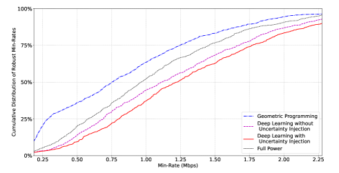
Figure 7: Cumulative distribution of robust minimum-rates in D2D wireless networks under test setting B.

As shown in these results, under various interference levels, link densities, and transceiver distance distributions, the neural network trained with uncertainty injection consistently produces more robust solutions. The performance gain due to the proposed uncertainty injection training is up to 9%, as compared to a deep neural network without uncertainty injection. The gain is much higher, in the range of 48-66%, when compared with the geometric programming benchmark, which is a globally optimal solution that does not account for channel uncertainty. In fact, geometric programming does not even perform as well as simply using full power in term of the robust minimum rate, although as expected it does much better in term of nominal minimum rate.

VII Conclusion

This paper proposes a novel uncertainty injection training method for deep learning models to perform robust optimization against parameter uncertainties. We consider a robust optimization problem that aims to compute robust solutions based only on the measured or the estimated problem parameters, while can still perform well with parameter uncertainties. Traditional robust optimization techniques addressing such problems require complicated mathematical characterizations of the parameter uncertainties, which are often difficult to analyze and may not reflect realistic environments accurately. Instead, sample-based uncertainty modeling is an attractive alternative because of its simplicity and accuracy.

The proposed training scheme utilizes the capability of deep neural networks to learn from samples of uncertainties. By injecting uncertainties, an empirical estimate of the robust objective can be obtained and used for updating the neural network model parameter during training. The proposed uncertainty injection scheme are applicable to a variety of robust optimization problems, while having low computational complexity. To illustrate the effectiveness of this method, we present promising numerical simulation results on two wireless communication applications. We believe that the proposed method opens up an avenue for wider application of deep learning based robust optimization under realistic scenarios, where uncertainties are ubiquitous and highly agnostic.

References

- [1] W. Cui, K. Shen, and W. Yu, “Deep learning for robust power control for wireless networks,” in IEEE Int. Conf. Acoust. Speech Signal Process. (ICASSP), May 2020.
- [2] A. Krizhevsky, I. Sutskever, and G. E. Hinton, “Imagenet classification with deep convolutional neural networks,” in Adv. Neural Inf. Process. Syst. (NIPS), Dec. 2012.
- [3] A. L. Maas, R. E. Daly, P. T. Pham, D. Huang, A. Y. Ng, and C. Potts, “Learning word vectors for sentiment analysis,” in Annu. Meeting Assoc. Comput. Linguistics (ACL), Jun. 2011, pp. 142–150.
- [4] K. He, X. Zhang, S. Ren, and J. Sun, “Deep residual learning for image recognition,” in IEEE Conf Comput. Vision Pattern Recognit. (CVPR), Jun. 2016.
- [5] D. P. Kingma and M. Welling, “Auto-encoding variational bayes,” in Int. Conf. Learn. Representations (ICLR), Apr. 2014.
- [6] I. Goodfellow, J. Pouget-Abadie, M. Mirza, B. Xu, D. Warde-Farley, S. Ozair, A. Courville, and Y. Bengio, “Generative adversarial nets,” in Adv. Neural Inf. Process. Syst. (NIPS), Dec. 2014.
- [7] A. Radford, L. Metz, and S. Chintala, “Unsupervised representation learning with deep convolutional generative adversarial networks,” in Int. Conf. Learn. Representations (ICLR), May 2016.
- [8] K. Gregor and Y. LeCun, “Learning fast approximations of sparse coding,” in Int. Conf Mach. Learn. (ICML), Jun. 2010, pp. 399–406.
- [9] H. Sun, X. Chen, Q. Shi, M. Hong, X. Fu, and N. D. Sidiropoulos, “Learning to optimize: Training deep neural networks for interference management,” IEEE Trans. Signal Process., vol. 66, no. 20, pp. 5438–5453, Aug. 2018.
- [10] W. Cui, K. Shen, and W. Yu, “Spatial deep learning for wireless scheduling,” IEEE J. Sel. Areas Commun., vol. 37, pp. 1248–1261, Jun. 2019.
- [11] C. Szegedy, W. Zaremba, I. Sutskever, J. Bruna, D. Erhan, I. Goodfellow, and R. Fergus, “Intriguing properties of neural networks,” in Int. Conf. Learn. Representations (ICLR), Apr. 2014.
- [12] A. Fawzi, S. Moosavi-Dezfooli, and P. Frossard, “Robustness of classifiers: from adversarial to random noise,” in Adv. Neural Inf. Process. Syst. (NIPS), Dec. 2016, pp. 1632–1640.
- [13] N. Natarajan, I. S. Dhillon, P. Ravikumar, and A. Tewari, “Learning with noisy labels,” in Adv. Neural Inf. Process. Syst. (NIPS), Dec. 2013.
- [14] A. Joulin, L. van der Maaten, A. Jabri, and N. Vasilache, “Learning visual features from large weakly supervised data,” in Eur. Conf. Comput. Vision (ECCV), Nov. 2015.
- [15] A. Veit, N. Alldrin, G. Chechik, I. Krasin, A. Gupta, and S. Belongie, “Learning from noisy large-scale datasets with minimal supervision,” in IEEE Conf Comput. Vision Pattern Recognit. (CVPR), Jul. 2017, pp. 839–847.
- [16] D. Rolnick, A. Veit, S. Belongie, and N. Shavit, “Deep learning is robust to massive label noise,” 2017, [Online] Available: https://arxiv.org/pdf/1705.10694.pdf.
- [17] A. Sinha, H. Namkoong, R. Volpi, and J. Duchi, “Certifying some distributional robustness with principled adversarial training,” 2017, [Online] Available: https://arxiv.org/pdf/1710.10571.pdf.
- [18] G. Pleiss, M. Raghavan, F. Wu, J. Kleinberg, and K. Q. Weinberger, “On fairness and calibration,” in Adv. Neural Inf. Process. Syst. (NIPS), Dec. 2017.
- [19] J. Duchi and H. Namkoong, “Variance-based regularization with convex objectives,” J. Mach. Learn. Res. (JMLR), vol. 20, no. 1, pp. 2450–2504, Jan. 2019.
- [20] M. Hein, M. Andriushchenko, and J. Bitterwolf, “Why relu networks yield high-confidence predictions far away from the training data and how to mitigate the problem,” in IEEE Conf. Comput. Vision Pattern Recognit. (CVPR), Jun. 2019, pp. 41–50.
- [21] J. Fan, Y. Shen, N. Zhou, and Y. Gao, “Harvesting large-scale weakly-tagged image databases from the web,” in IEEE Conf. Comput. Vision Pattern Recognit. (CVPR), Jun. 2010.
- [22] V. Ordonez, G. Kulkarni, and T. Berg, “Im2text: Describing images using 1 million captioned photographs,” in Adv. Neural Inf. Process. Syst. (NIPS), Dec. 2011, pp. 1143–1151.
- [23] Y. Xia, X. Cao, F. Wen, and J. Sun, “Well begun is half done: Generating high-quality seeds for automatic image dataset construction from web,” in Eur. Conf. Comput. Vision (ECCV), Sep. 2014, pp. 387–400.
- [24] S. Gu and L. Rigazio, “Towards deep neural network architectures robust to adversarial examples,” in Int. Conf. Learn. Representations (ICLR), May 2015.
- [25] C. M. Bishop, “Training with noise is equivalent to tikhonov regularization,” Neural Comput., vol. 7, no. 1, pp. 108–116, Jan. 1995.
- [26] R. D. Reed and R. J. Marks, II, Neural Smithing: Supervised Learning in Feedforward Artificial Neural Networks. Bradford Books, Feb. 1999.
- [27] U. Shaham, Y. Yamada, and S. Negahban, “Understanding adversarial training: Increasing local stability of neural nets through robust optimization,” 2015, [Online] Available: https://arxiv.org/pdf/1511.05432.pdf.
- [28] S. Moosavi-Dezfooli, A. Fawzi, and P. Frossard, “Deepfool: a simple and accurate method to fool deep neural networks,” in IEEE Conf Comput. Vision Pattern Recognit. (CVPR), Jun. 2016.
- [29] A. Madry, A. Makelov, L. Schmidt, D. Tsipras, and A. Vladu, “Towards deep learning models resistant to adversarial attacks,” in Int. Conf. Learn. Representations (ICLR), May 2018.
- [30] A. Graves, A. Mohamed, and G. Hinton, “Speech recognition with deep recurrent neural networks,” in IEEE Int. Conf. Acoust., Speech, and Signal Process. (ICASSP), May 2013.
- [31] B. Poole, J. Sohl-Dickstein, and S. Ganguli, “Analyzing noise in autoencoders and deep networks,” Jun. 2014, [Online] Available: https://arxiv.org/pdf/1406.1831.pdf.
- [32] C. Gulcehre, M. Moczulski, M. Denil, and Y. Bengio, “Noisy activation functions,” in Int. Conf. Mach. Learn. (ICML), Jun. 2016.
- [33] A. Neelakantan, L. Vilnis, Q. V. Le, I. Sutskever, L. Kaiser, K. Kurach, and J. Martens, “Adding gradient noise improves learning for very deep networks,” Nov. 2015, [Online] Available: https://arxiv.org/pdf/1511.06807.pdf.
- [34] M. Zhou, T. Liu, Y. Li, D. Lin, E. Zhou, and T. Zhao, “Towards understanding the importance of noise in training neural networks,” in Int. Conf. Mach. Learn. (ICML), Jun. 2019.
- [35] X. Wu, S. Tavildar, S. Shakkottai, T. Richardson, J. Li, R. Laroia, and A. Jovicic, “FlashLinQ: A synchronous distributed scheduler for peer-to-peer ad hoc networks,” IEEE/ACM Trans. Netw., vol. 21, no. 4, pp. 1215–1228, Aug. 2013.
- [36] K. Shen and W. Yu, “FPLinQ: A cooperative spectrum sharing strategy for device-to-device communications,” in IEEE Int. Symp. Inf. Theory (ISIT), Jun. 2017, pp. 2323–2327.
- [37] Q. Shi, M. Razaviyayn, Z.-Q. Luo, and C. He, “An iteratively weighted MMSE approach to distributed sum-utility maximization for a MIMO interfering broadcast channel,” IEEE Trans. Signal Process., vol. 59, no. 9, pp. 4331–4340, Apr. 2011.
- [38] N. Naderializadeh and A. S. Avestimehr, “ITLinQ: A new approach for spectrum sharing in device-to-device communication systems,” IEEE J. Sel. Areas Commun., vol. 32, no. 6, pp. 1139–1151, Jun. 2014.
- [39] B. Zhuang, D. Guo, E. Wei, and M. L. Honig, “Scalable spectrum allocation and user association in networks with many small cells,” IEEE Trans. Commun., vol. 65, no. 7, pp. 2931–2942, Jul. 2017.
- [40] I. Rhee, A. Warrier, J. Min, and L. Xu, “DRAN: Distributed randomized TDMA scheduling for wireless ad hoc networks,” IEEE Trans. Mobile Comput., vol. 8, no. 10, pp. 1384–1396, Oct. 2009.
- [41] L. P. Qian and Y. J. Zhang, “S-MAPEL: Monotonic optimization for non-convex joint power control and scheduling problems,” IEEE Trans. Wireless Commun., vol. 9, no. 5, pp. 1708–1719, May 2010.
- [42] M. Johansson and L. Xiao, “Cross-layer optimization of wireless networks using nonlinear column generation,” IEEE Trans. Wireless Commun., vol. 5, no. 2, pp. 435–445, Feb. 2006.
- [43] M. B. Shenouda and T. N. Davidson, “Convex conic formulations of robust downlink precoder designs with quality of service constraints,” IEEE J. Sel. Topics Signal Process., vol. 1, no. 4, pp. 714–724, Dec. 2007.
- [44] M. Hasan, E. Hossain, and D. I. Kim, “Resource allocation under channel uncertainties for relay-aided device-to-device communication underlaying LTE-A cellular networks,” IEEE Trans. Wireless Commun., vol. 13, no. 4, pp. 2322–2338, Mar. 2014.
- [45] Y. Shen and K. S. Kwak, “Robust power control for cognitive radio networks with proportional rate fairness,” ICT Express, vol. 1, pp. 22–25, June 2015.
- [46] W. Wu, R. Liu, Q. Yang, and T. Q. S. Quek, “Learning-based robust resource allocation for D2D underlaying cellular network,” IEEE Trans. Wireless Commun., vol. 21, no. 8, pp. 6731–6745, Aug. 2022.
- [47] J. Wang, J. Chen, Y. Lu, M. Gerla, and D. Cabric, “Robust power control under location and channel uncertainty in cognitive radio networks,” IEEE Wireless Commun. Lett., vol. 2, no. 4, pp. 113–116, April 2015.
- [48] E. Dall’Anese, S. Kim, G. B. Giannakis, and S. Pupolin, “Power control for cognitive radio networks under channel uncertainty,” IEEE Trans. Wireless Commun. , vol. 10, no. 10, pp. 3541 – 3551, August 2011.
- [49] B. K. Chalise, S. Shahbazpanahi, A. Czylwik, and A. B. Gershman, “Robust downlink beamforming based on outage probability specifications,” IEEE Trans. Wireless Commun., vol. 6, no. 10, pp. 3498–3503, Oct. 2007.
- [50] M. B. Shenouda and T. N. Davidson, “Probabilistically-constrained approaches to the design of the multiple antenna downlink,” in Asilomar Conf. Signals Syst. Comput., Oct. 2008.
- [51] K. Wang, A. M. So, T. Chang, W. Ma, and C. Chi, “Outage constrained robust transmit optimization for multiuser MISO downlinks: Tractable approximations by conic optimization,” IEEE Trans. Signal Process., vol. 62, no. 21, pp. 5690–5705, Nov. 2014.
- [52] F. Sohrabi and T. N. Davidson, “Coordinate update algorithms for robust power loading for the MU-MISO downlink with outage constraints,” IEEE Trans. Signal Process., vol. 64, no. 11, pp. 2761–2773, Jan. 2016.
- [53] M. Medra and T. N. Davidson, “Per-user outage-constrained power loading technique for robust MISO downlink,” in Asilomar Conf. Signals Syst. Comput., Nov. 2015.
- [54] M. Elnourani, S. Deshmukh, B. Beferull-Lozano, and D. Romero, “Robust underlay device-to-device communications on multiple channels,” Feb. 2020, [Online] Available: https://arxiv.org/pdf/2002.11500.pdf.
- [55] P. de Kerret and D. Gesbert, “Robust decentralized joint precoding using team deep neural network,” in Int. Symp. Wireless Commun. Syst. (ISWCS), Aug. 2018.
- [56] J. Kim, H. Lee, and S. Park, “Learning robust beamforming for MISO downlink systems,” IEEE Commun. Lett., vol. 25, no. 6, pp. 1916–1920, Mar. 2021.
- [57] R. Dong, B. Wang, and K. Cao, “Deep learning driven 3D robust beamforming for secure communication of UAV systems,” IEEE Wireless Commun. Lett., vol. 10, no. 8, pp. 1643–1647, Aug. 2021.
- [58] B. Sklar, “Rayleigh fading channels in mobile digital communication systems Part I: Characterization,” IEEE Commun. Mag., vol. 35, no. 7, pp. 90–100, Jul. 1997.
- [59] C. B. Peel, B. M. Hochwald, and A. L. Swindlehurst, “A vector-perturbation technique for near-capacity multiantenna multiuser communication-part i: channel inversion and regularization,” IEEE Trans. Commun., vol. 53, no. 1, pp. 195–202, Jan. 2005.
- [60] J. Kiefer and J. Wolfowitz, “Stochastic estimation of the maximum of a regression function,” Ann. Math. Statist., vol. 23, no. 3, pp. 462–466, Sep. 1952.
- [61] D. E. Goldberg and J. H. Holland, “Genetic algorithms and machine learning,” Mach. Learn., vol. 3, pp. 95–99, Oct. 1988.
- [62] C. Lee, S. Xie, P. Gallagher, Z. Zhang, and Z. Tu, “Deeply-supervised nets,” in Int. Conf. Artif. Intell. Statist. (AISTATS), May 2015.
- [63] A. Paszke et al., “PyTorch: An imperative style, high-performance deep learning library,” in Adv. Neural Inf. Process. Syst. (NeurIPS), Dec. 2019, pp. 8024–8035.
- [64] M. Abadi et al., “TensorFlow: Large-scale machine learning on heterogeneous systems,” 2015, software available from tensorflow.org. [Online]. Available: https://www.tensorflow.org/
- [65] W. R. V. Zwet, Convex Transformations of Random Variables. Amsterdam, Netherlands: Mathematisch Centrum, 1964, ch. 3.
- [66] G. Chatillon, R. Gelinas, L. Martin, and L. Laurencelle, “When is it preferable to estimate population percentiles from a set of classes rather than from the raw data?” J. Educ. Statist., vol. 12, no. 4, pp. 395–409, 1987.
- [67] H. V. Poor, An Introduction to Signal Detection and Estimation, 2nd ed. New York, NY, USA: Springer Science & Business Media, Feb. 1994.
- [68] M. Chiang, C. W. Tan, D. P. Palomar, D. O’Neill, and D. Julian, “Power control by geometric programming,” IEEE Trans. Wireless Commun., vol. 6, no. 7, pp. 2640–2651, Jul. 2007.