An Aligned Multi-Temporal Multi-Resolution Satellite Image Dataset for Change Detection Research

Abstract

This paper presents an aligned multi-temporal and multi-resolution satellite image dataset for research in change detection. We expect our dataset to be useful to researchers who want to fuse information from multiple satellites for detecting changes on the surface of the earth that may not be fully visible in any single satellite. The dataset we present was created by augmenting the SpaceNet-7 dataset [22] with temporally parallel stacks of Landsat and Sentinel images. The SpaceNet-7 dataset consists of time-sequenced Planet images recorded over 101 AOIs (Areas-of-Interest). In our dataset, for each of the 60 AOIs that are meant for training, we augment the Planet datacube with temporally parallel datacubes of Landsat and Sentinel images. The temporal alignments between the high-res Planet images, on the one hand, and the Landsat and Sentinel images, on the other, are approximate since the temporal resolution for the Planet images is one month — each image being a mosaic of the best data collected over a month. Whenever we have a choice regarding which Landsat and Sentinel images to pair up with the Planet images, we have chosen those that had the least cloud cover. A particularly important feature of our dataset is that the high-res and the low-res images are spatially aligned together with our MuRA framework presented in this paper. Foundational to the alignment calculation is the modeling of inter-satellite misalignment errors with polynomials as in NASA’s AROP [8] algorithm. We have named our dataset MuRA-T for the MuRA framework that is used for aligning the cross-satellite images and ”T” for the temporal dimension in the dataset.

1 Introduction

Satellites are a rich source of data for identifying and tracking significant changes on the surface of the earth. Such changes are of great concern to a large variety of people and that includes scientists, urban planners, those engaged in damage assessment and mitigation planning when natural disasters strike, etc.

For obvious reasons, detecting change requires at least two images, before and after the event that is believed to have caused the change. More generally, if the goal is to understanding the temporal evolution of the change taking place, one would want a sequence of images in the form of a time series for the same geographical region on the ground.

Such time series sequences of images can now be constructed at medium resolution (around 4m) with the data made available by Planet. As demonstrated by the SpaceNet-7 dataset, this resolution is adequate for identifying and tracking changes related to buildings in urban areas. For each geographic area, the SpaceNet-7 dataset contains Planet images, one per month (that may not always be consecutive), over a span of around 24 months.

While SpaceNet-7 is a huge step forward in what’s needed for developing algorithms that can track changes at the granularity of individual buildings in an urban area, our own interest includes the geographic context of the urban areas that contain the buildings. That is, we are as interested in the changes taking place in the landmasses surrounding the buildings as we are in the purely urban scenes consisting of just the buildings.

To that end, our dataset augments the SpaceNet-7 dataset with temporally parallel Landsat and Sentinel datacubes of images. That is, for each Planet image in a temporal stack, our dataset provides a Landsat image and a Sentinel image at roughly the same time. Each Planet image in the stack represents the best of the Planet data captures over a period of one month. In other words, a Planet image is not an instantaneous snapshot of what is on the ground, but a mosaic of the best of what was seen at each point on the ground during a span of one month. In keeping with this spirit, when we choose a low-res image, Landsat or Sentinel, to go along with a Planet image, we try to choose the best of the low-res images during that month on the basis of primarily the extent of the cloud cover.

What makes our dataset special is the fact that the low-res images, Landsat and Sentinel, are spatially aligned with the Planet images. Since the images from the different satellites are at different resolutions, one of the first steps in the alignment process is deciding what working resolution to use for all the images for the purpose of data alignment.

For aligning images from any pair of disparate satellites, we have three choices: (1) Downsample the high-res images so that its new sampling rate corresponds to that of the low-res images; (2) Use super-resolution or image-to-image translation neural networks to upsample the low-res images so that its sampling rate corresponds to that of the high-res images; and (3) Use a combination of downsampling and upsampling for all the images from the different satellites to correspond to some common agreed-upon sampling rate. As to which of these strategies to use depends on the scale at which one would like to detect temporal changes on the ground. For the version of the dataset we are providing at the moment, the alignment is carried out by downsampling the Planet images to correspond to the sampling rates of the Landsat and Sentinel data.

Our basic logic for cross-satellite image alignment was inspired by NASA’s AROP [8] algorithm in which the misalignment errors are modeled by a polynomial. The degree of this polynomial can be adapted to the required alignment precision. In the current dataset, the alignment accuracy was measured by the reprojection error for the largest possible inlier set of the corresponding tie-points between the two images being aligned with each other. This is a standard approach to measuring the misalignment error between a pair of images on a relative basis — meaning just with respect to each other as opposed to also with respect to the features on the ground. In future versions of our dataset, our performance numbers related to alignment precision will be augmented with those that describe absolute accuracy with respect to the ground control points (GCP) in those geographic regions where such land references are available. As reported in Sec. 7, all our reprojection-error based alignment accuracies are at the sub-pixel level.

The cross-satellite image alignment process as described above was carried out with an algorithmic framework that, for convenience, we have named MuRA for “Multi-Resolution Alignment”. Since MuRA has played a central role in the creation of our dataset, we have named it the MuRA-T Dataset in which “T” refers to the temporal dimension of the data. To the best of what we know, MuRA-T is the first temporally and spatially aligned multi-satellite dataset that can be used for change detection research.

In the rest of the paper, Sec. 2 presents a brief literature survey of the different datasets currently available for satellite images and the computational models that can be used for aligning the same-satellite and cross-satellite images. Since our dataset is an augmentation of the SpaceNet-7 dataset, we devote Sec. 3 to presenting the relevant highlights of this well-known dataset and asking the reader to consult the original SpaceNet-7 paper for the details. Sec. 4 presents a summary of the more significant attributes of the Landsat and Sentinel images that are relevant to how we have created our dataset. Sec. 5 presents the “mechanics” of how we accessed the different repositories on the internet for constructing the MuRA-T dataset. Sec. 6 present the MuRA logic that was used for spatially aligning the images in MuRA-T. The alignment results are presented in Sec. 7.

2 Literature Survey

This section first briefly reviews several other publicly available datasets of satellite images while, at the same time, pointing out how MuRA-T differs from them. Following that, we present a brief review of the image alignment algorithms for satellite images.

2.1 Satellite Image Datasets

The satellite image datasets that have received the most attention during the last few years are those related to the various SpaceNet challenges. The paper by Van Etten et al. [6] provides a nice review of the datasets created for the first three challenges and the evaluation metrics used. In these datasets, consisting of time-static imagery, the focus was primarily on either just building extraction or the extraction of both buildings and roads from high-res imagery. WorldView images proved ideal for these datasets because of the high ground resolution (30cm and 50cm) and the high quality of the images. Creating the ground truth labels for the buildings (and roads) required semi-automated processing of the data.

The three datasets used in the DeepGlobe challenge [4] were meant for three different tasks: building detection, road extraction, and landcover classification. Of the datasets provided, the one for building detection is actually from the SpaceNet collection. For road extraction and landcover classification, the datasets provided were based on DigitalGlobe+Vivid imagery.

There is also the multi-view satellite dataset presented in [23] for the development of algorithms that can work directly with off-nadir satellite images. The data is based on WorldView-2 images at 50cm resolution. The off-nadir look angles in this data range from directly overhead to $54^{\circ}$ elevation. This static-time dataset was again meant for solving the building detection problem, but in off-nadir imagery.

There is also the SpaceNet-6 satellite image dataset designed for developing and testing object detection algorithms under all-weather conditions [18]. What makes this dataset distinctive is that it includes both optical and SAR (Synthetic Aperture Radar) imagery. An interesting insight gained from this dataset was that the object detection algorithms that are pre-trained with optical images and then further trained on SAR images outperform the algorithms that have only the SAR data to work with.

Another interesting satellite image dataset is the xBD dataset [10] meant specifically for developing algorithms for assessing damage to buildings. The dataset consists of before-and-after images from 19 natural disaster sites and was sourced from Maxar’s Open Data program. There is also the EarthNet 2021 dataset [14] that contains Sentinel-2 imagery over a span of several months for predicting localized climate changes. Although temporal, this dataset does not provide multi-satellite data like what we do.

That brings us to the SpaceNet-7 [22] dataset that contains 101 AOIs, 60 for training and the rest for testing and validation, of Planet imagery over roughly a 24-month period. On account of the importance of this dataset to our own, we have devoted a separate section to it, Sec. 3.

2.2 Image Alignment

When dealing with multi-view images, the algorithms that have proved most effective for aligning a mix of images over the same geographic area are based on the RPC (Rational Polynomial Coefficient) model for the satellite cameras and the logic of bundle-adjustment [20] [11] for the actual alignment. Although the RPC model has 78 polynomial coefficients as parameters, Grodecki & Dial [9] have demonstrated that the misalignment error in satellite images can be corrected by estimating only the bias correction terms in the RPC model.

When the images to be aligned involve only the nadir views of the earth — as is the case with the Planet images and the low-res Landsat and Sentinel images — the misalignment errors are more easily modeled as affine transformations or, equivalently, as polynomial warps as in NASA’s AROP[8] algorithm. We use the same approach for modeling the misalignment errors in our cross-satellite image alignment work presented in this paper.

3 The SpaceNet-7 Dataset

As mentioned previously, the dataset we present in this paper, MuRA-T, is an augmentation of the SpaceNet-7 dataset. Therefore, a few comments about the SpaceNet-7 dataset are in order.

SpaceNet-7 consists of publicly available sequences of Planet images, with each image representing the best of the satellite captures over one month for the geographic area in question. This creates a temporal stack of images as shown in Fig. 1, also referred to as a datacube, with a time resolution of one month (nominally speaking). SpaceNet-7 provides such datacubes for 101 AOIs around the globe. Of these, the data over 60 AOIs is meant to be used for training, and the rest for testing and validation. On the average, each temporal stack spans roughly 24 months. The images in each stack are on-nadir and are based on the data in the RGB bands with a spatial resolution of roughly 4m on the ground. At this time, our dataset, MuRA-T, is based on just the 60 AOIs that are meant for training.

Since SpaceNet-7 is an “urban development” dataset, one of its important goals is to promote research in building detection algorithms. To that end, SpaceNet-7 provides high-quality building annotations in all the images in the dataset, with each building getting a separate label that can be tracking in time. The dataset comes with a footprint mask for each building. Each image also comes with an “unusable data mask” to designate the pixel blobs that are not trusted on account of either the remaining cloud cover in the images or because of unacceptable geo-reference errors. There are between 10,000 and 20,000 building annotations in each image.

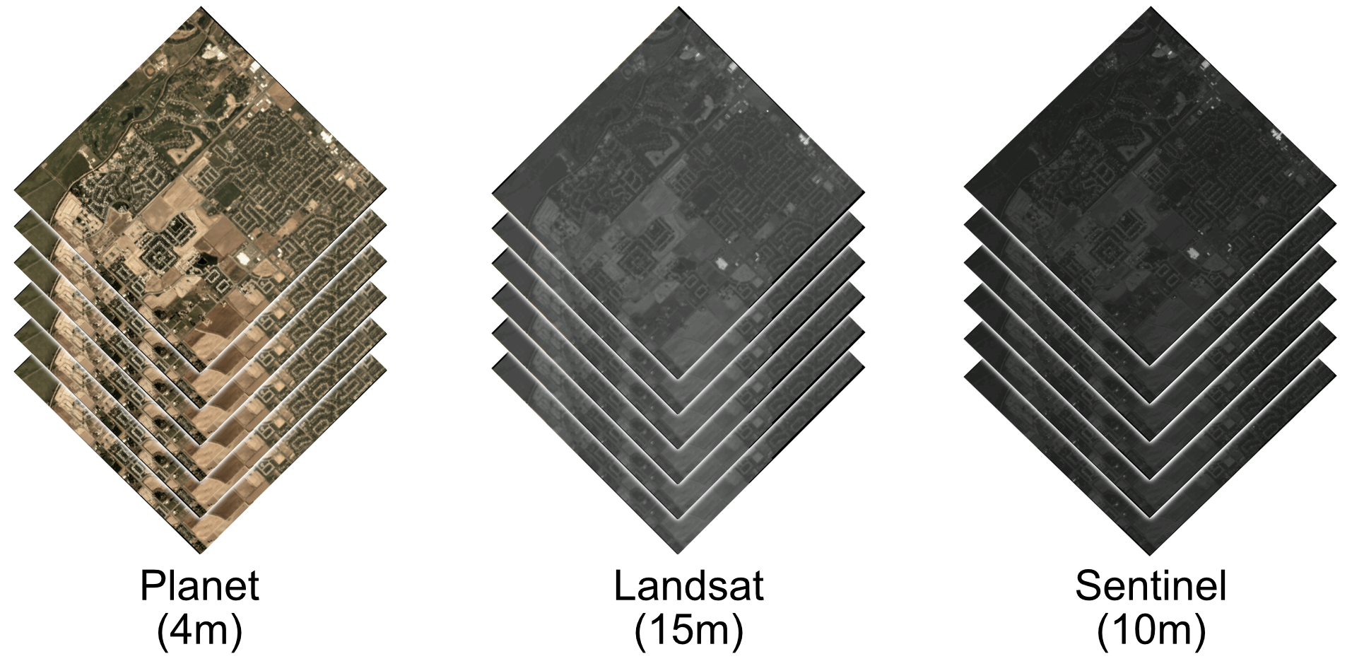
Figure 1: Three temporally paralleled and spatially aligned datacubes. The left datacube represents a stack of SpaceNet-7 Planet images, the center a stack of Landsat-8 images, and the right a stack of Sentinel-2 images.

4 Some Relevant Attributes of the Landsat and Sentinel Imagery

As mentioned in the Introduction, our own research interests go beyond just building detection — we are also interested in the geographic context of the buildings. That is, we are as interested in the changes taking place in the landmasses surrounding the buildings as in the purely urban scenes consisting of just the buildings.

That’s our main reason for augmenting the temporal stacks of the Planet images in SpaceNet-7 with temporally parallel stacks of Landsat and Sentinel images. Since each Planet image represents the best of the satellite captures over one month, it makes sense to pair each Planet image with the best possible Landsat image and the best possible Sentinel image recorded during the same month. By “best possible”, we mean the Landsat and Sentinel images with the least cloud cover. That’s exactly what we have done in our MuRA-T dataset. We used the F-MASK algorithm [24] for cloud detection.

Our augmentation of SpaceNet-7 with Landsat and Sentinel images constitutes — to the best of our knowledge — a first attempt at the creation of a temporally and spatially aligned dataset of images from multiple satellites. For obvious reasons, this is going to lead to new opportunities in research, in the sense that it would allow researches to formulate more complex problems in change detection whose solutions require data from multiple satellites simultaneously. Any algorithm development along these lines would need to address the challenges created by the fact that the images from the different satellites are likely to sample the points on the ground at very different spatial resolutions.

What makes the issue of having to deal with different ground-sampling resolutions in different satellites even more interesting is the fact there is no single value for this spatial resolution for any given earth observation satellite. The data produced by such satellites is always multi-spectral and each spectral band is characterized by its own ground-sampling resolution value. Tabs. 1 and 2 are a listing of the different spectral bands imaged by the Landsat and Sentinel satellites and their per pixel ground sampling resolution values.

Comparing the data presented in these two tables, the highest ground sampling resolution value for Landsat-8 – 15m – is for the Panchromatic (“Pan” for short) band and the same for Sentinel-2 is for the RGB bands, at 10m.

Band	Band Description	Band wavelength
No		range ($\mu$m)
1	30 m Coastal/Aerosol	0.435-0.451
2	30 m Blue	0.452-0.512
3	30 m Green	0.533-0.590
4	30 m Red	0.636-0.673
5	30 m Near-Infrared (NIR)	0.851-0.879
6	30 m Short Wavelength Infrared (SWIR)	1.566-1.651
7	30 m SWIR 2	2.107-2.294
8	15 m Panchromatic	0.503-0.676
9	30 m Cirrus	1.363-1.384
10	100 m Thermal Infrared Sensor (TIRS) 1	10.60-11.19
11	100 m TIRS 2	11.50-12.51

Table 1: Landsat-8 band details

Band	Band Description	Central	Bandwidth
No		Wavelength	(nm)
		(nm)
1	60 m Ultra blue	442.7	21
2	10 m Blue	492.4	66
3	10 m Green	559.8	36
4	10 m Red	664.6	31
5	20 m Visible and Near-Infrared (VNIR)	704.1	15
6	20 m VNIR	740.5	15
7	20 m VNIR	782.8	20
8	10 m VNIR	832.8	106
8a	20 m VNIR	864.7	21
9	60 m Short Wavelength Infrared (SWIR)	945.1	20
10	60 m SWIR	1373.5	31
11	20 m SWIR	1613.7	91
12	20 m SWIR	2202.4	175

Table 2: Sentinel-2 band details

5 Creating Temporally Paralleled Landsat And Sentinel Datacubes

As one might expect, the key to temporally pairing low-resolution data with the Planet images in the SpaceNet-7 stacks is finding Landsat and Sentinel images at the same location and at times that correspond to the month designators for the Planet images. As it turns out, the Lat/Long coordinates of each AOI are sufficient for finding the corresponding Landsat images from the AWS Registry of Open Data for these images [13].

Images in the AWS Landsat registry are cataloged by their WRS2 path and rows index values. Each image is tagged with its acquisition date. Given the Lat/Long coordinates associated with a Planet image, it is relatively straightforward to find its corresponding WRS2 path and row values. We automated this process by writing a Python script that compares the corner coordinates of each SpaceNet-7 AOI with the WRS2 path and row shapefile provided by NASA [21]. Using the metadata list for all Landsat scenes in the AWS registry, the URLs to the relevant Landsat images can be found easily and, through those URLs, the images can be downloaded with the AWS CLI. In terms of their sizes, the SpaceNet-7 AOIs are much smaller than the Landsat tiles. Therefore, in MuRA-T, the downloaded Landsat images are clipped in order to correspond to the AOIs.

Sentinel-2 images were accessed in a similar manner using the Google Cloud Platform with the help of BigQuery API. Using these APIs, any Sentinel-2 imagery matching the SpaceNet-7 AOIs dates and locations can be downloaded with the help of a custom python script.

6 Spatially Aligning the Multi-Res Images

If the goal is to draw inferences from the data coming from multiple satellites, each satellite characterized by its own ground sampling distance, it is important for the multi-satellite images at each time step to be aligned with one another. Applications such as change detection can be sensitive to even the slightest misalignments. The goal is always to align the images with as high a sub-pixel precision as possible. To that end, we have developed a framework of algorithms, named MuRA, for aligning together multi-resolution images. MuRA includes paths for using super-resolution and image-to-image translation networks for upsampling the low-res images to high-res. The different processing pathways in MuRA allow for the following three different possibilities for cross-satellite image alignment:

1. In a mix of images from different satellites, we can downsample all the images so that their ground sampling resolution corresponds to that of the lowest-resolution images. For example, when aligning a 4m Planet image with a 15m Landsat image, we would first downsample the Planet image to a 15m resolution. We can think of this as the least common denominator approach to dealing with the alignment of multi-res images.

2. There is a second possibility and that is a result of the rapid advances that are currently being made in super-resolution and image-to-image translation networks. This possibility would call for upsampling the lower resolution images to that of the highest-resolution image and then applying the alignment logic to the data. When using super-resolution networks, the goal would be to make fuzzy details look sharper — in the same sense as in the more traditional super-resolution algorithms that manipulate the Fourier transform of an image by raising the transform values near the limits of the Nyquist criterion. On the other hand, when using image-to-image translation networks, one can imbue lower-resolution images with aspects of structural sharpness as learned from the higher resolution images. MuRA incorporates both types of these neural networks.

3. The third possibility is to use a combination of upsampling and downsampling. This approach would be appropriate for situations when the resolution difference between the highest-res and the lowest-res images in the mix is much too large to handle with the either of the above two approaches.

In the MuRA-T dataset being made available, we have only used the processing path of MuRA for the first possibility described above. That is, for the version of the dataset we are providing at the moment, the alignment is carried out by downsampling the Planet images to correspond to the sampling rates of the Landsat and Sentinel data.

6.1 The MuRA Pathways Used in the MuRA-T Dataset

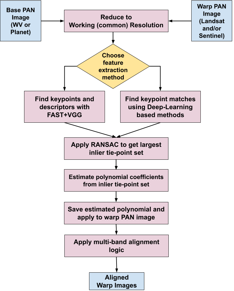
Figure 2: The computational pathway of the MuRA framework used for constructing the MuRA-T dataset.

Fig. 2 shows the section of the MuRA framework used for constructing the MuRA-T dataset. First, the higher resolution image is downsampled so each image is at a common working resolution (i.e. the lowest resolution among the input images). Once re-sampled, we obtain tiepoints using one of several possible feature extraction and matching methods. Our framework is based on a plug-n-play design that makes it easy for us to test different possible feature extraction and the feature matching methods for image alignment. We used both FAST+VGG [15, 19] and SuperPoint+SuperGlue [5, 17] algorithms for the alignments needed for MuRA-T because these algorithms yielded the best results. Further details are presented in Sec. 6.3.

Once we obtain a set of tiepoints through feature matching, we apply bundle adjustment [20] to this set in order to estimate the coefficients of the polynomial model used for the misalignment error. An important component of the bundle-adjustment logic is the RANSAC algorithm [7] for outlier rejection. RANSAC is invoked iteratively in order to find the largest inlier set of tiepoints for aligning a pair of images. The nature of the polynomial model is described in Sec. 6.2. Using the estimated polynomial model, we re-sample the misaligned low-resolution image into an aligned image.

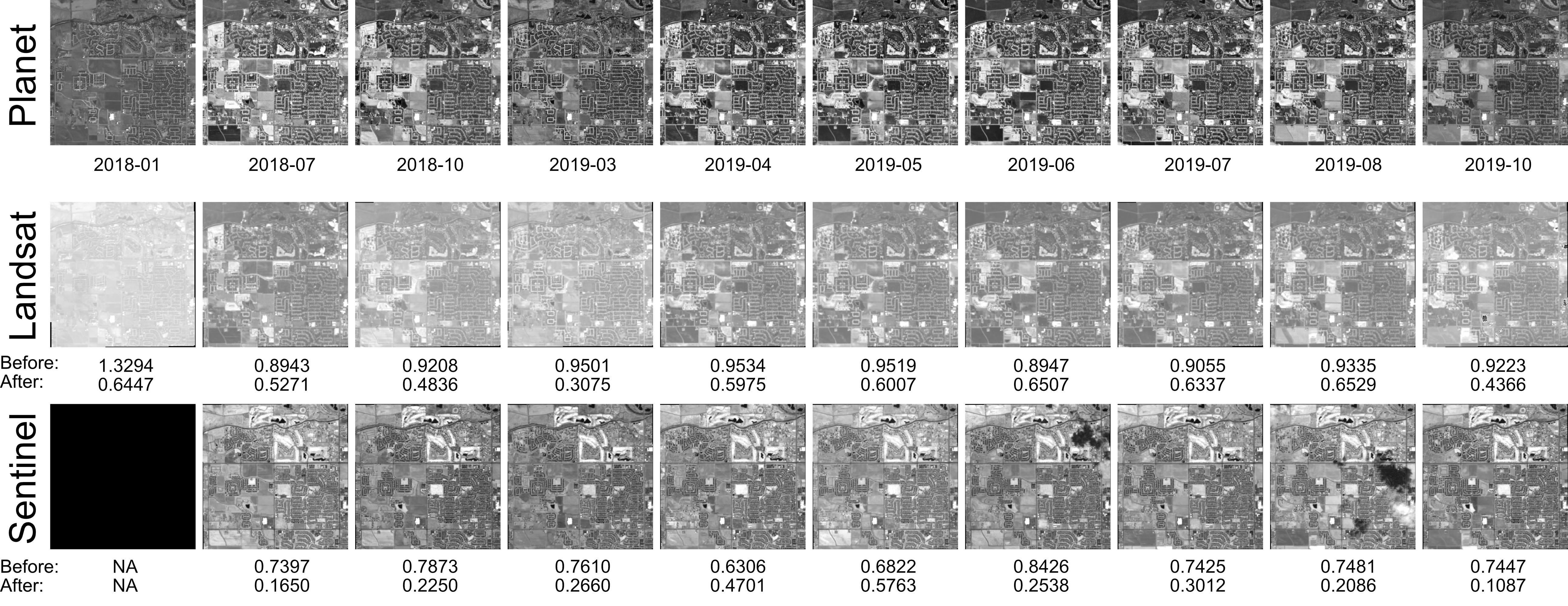
Figure 3: Shown in the top row are 10 of the 24 Planet images for the Meridian, Idaho, AOI. On account of the space constraints, we have shown only the first ten images in the Planet stack over the AOI. Note the Planet images in the SpaceNet-7 stacks are not always for consecutive months, as one can tell from month/year tags shown below the Planet images. The second row shows the aligned Landsat images and the third row the aligned Sentinel images. The Landsat and the Sentinel images were chosen as the best-of-the-month on the basis of containing the least cloud cover as detected by the F-MASK [24] algorithm. The before and after misalignment errors in terms of the RMSE values are also displayed for each of the images.

6.2 Modeling the Misalignment Error with Polynomials

Modeling of the misalignment errors in the alignment logic used for MuRA-T is based on NASA’s AROP [8] algorithm that was used to harmonize Landsat and Sentinel images into a single unified dataset. The polynomial correction model can essentially be thought of as an affine homography that is a relationship between the pixel coordinates of the corresponding pixel positions in a pair of images with the exception that the polynomial correction model can use higher degree polynomials unlike affine homographies. Shown below are the three choices for such polynomials. In the definitions shown, $(\hat{x}_{w},\hat{y}_{w})$ represent the warp image (meaning the misaligned image) pixel coordinates and $(x_{b},y_{b})$ the pixel coordinates in the base image (meaning the reference image).

Shift Correction Model:

$$\begin{split}\hat{x}_{w}&=a_{1}+x_{b}\\ \hat{y}_{w}&=b_{1}+y_{b}\end{split}$$ (1)

Affine Correction Model:

$$\begin{split}\hat{x}_{w}&=a_{1}+a_{2}x_{b}+a_{3}y_{b}\\ \hat{y}_{w}&=b_{1}+b_{2}x_{b}+b_{3}y_{b}\end{split}$$ (2)

Quadratic Polynomial Correction Model:

$$\begin{split}\hat{x}_{w}&=a_{1}+a_{2}x_{b}+a_{3}y_{b}+a_{4}x_{b}^{2}+a_{5}x_{b}y_{b}+a_{6}y_{b}^{2}\\ \hat{y}_{w}&=b_{1}+b_{2}x_{b}+b_{3}y_{b}+b_{4}x_{b}^{2}+b_{5}x_{b}y_{b}+b_{6}y_{b}^{2}\end{split}$$ (3)

The goal of alignment is to estimate the coefficients $\{a_{i}\}$ and $\{b_{i}\}$ given the corresponding tie points in the two images. This is accomplished by minimizing the distance between the actual measurements for the coordinates $(x_{w},y_{w})$ and their estimated values $(\hat{x}_{w},\hat{y}_{w})$ as yielded by the alignment algorithm — this distance is frequently referred to as the reprojection error. Formally, the minimization problem is stated as:

$$\begin{split}\{a_{i}^{*}\},\{b_{i}^{*}\}=\operatorname*{argmin}_{\{a_{i}\},\{b_{i}\}}\Big{\{}\sum_{k=0}^{N-1}(x_{w}^{(k)}-\hat{x}_{w}^{(k)})^{2}+\\ (y_{w}^{(k)}-\hat{y}_{w}^{(k)})^{2}\Big{\}}\end{split}$$ (4)

where $k$ is an index for a pair of tie-point correspondences among all the $N$ inliers used for computing the reprojection error. Fortunately, the problem in Eq. 4 can be easily converted to a linear least square problem as the polynomial correction model is a linear function of the parameters $\{a_{i}\}$ and $\{b_{i}\}$.

6.3 The Alignment Pipeline Used for MuRA-T

Since the new feature extraction and matching methods are being reported constantly, as previously stated, the computational steps in the image alignment pipeline shown in Fig. 2 are meant to operate on a plug-n-play basis. This has allowed us to experiment with a large number of possibilities for the feature extraction and feature matching steps in image alignment. The algorithms we tested include: SIFT [12], SURF [2], ORB [16], STAR+BRIEF [1, 3], FAST for feature extraction and VGG for matching, SuperPoint for feature extraction and SuperGlue for matching, etc. Of all these methods, we obtained the best results with FAST+VGG and SuperPoint+SuperGlue. These two approaches yielded the largest number of tiepoints between a pair of images on the average. While SuperPoint+SuperGlue is an end-to-end deep learning approach, FAST+VGG combines both traditional and deep learning-based methods towards the goal of feature extraction.

6.4 Resampling and Multi-Band Alignment

As discussed in Sec. 6.2, the correction model is a function of the base image coordinates at the working resolution. After determining the best polynomial for the PAN-to-PAN alignment between the reference image and the low-res image, next we need to align all the other bands of the warp image in question. To that end, each band of the warp image is aligned by modifying the PAN-to-PAN polynomial using the metadata for that band. This calculation requires us to go through several transformations as shown in Fig. 4. In this figure, “warp out” refers to the aligned version of the band image in question and “warp in” refers to the band image before alignment. Here is a listing of the computational steps:

1. For the pixel location in output warp image – warp-out – as shown in Fig. 4 we use the affine back projection function ($(\mathcal{P}_{aff}^{warp})^{-1}$) supplied by the metadata to get the corresponding 2D world location.

2. Using the 2D world location from the previous step, we project it into the working base image using the affine projection function, supplied again by the metadata, for the working base image ($\mathcal{P}_{aff}^{base}$) and obtain the pixel coordinate $(x_{b},y_{b})$.

3. Using the pixel coordinates of the working base and the polynomial correction model explained in Sec. 6.2, we identify the corrected warp pixel coordinates $(\hat{x}_{w},\hat{y}_{w})$.

4. Using the affine back projection function ($(\mathcal{P}_{aff}^{working\_warp})^{-1}$) of the working warp image, supplied by its metadata, we backproject the warp pixel coordinates $(\hat{x}_{w},\hat{y}_{w})$ to get their corresponding 2D world coordinates.

5. Finally, we project the 2D world coordinates from the previous step into the misaligned warp image, meaning the warp-in image, and obtain a pixel location. The value at this pixel location gets written into the output aligned warp image.

Using the above process we can produce resampled aligned images with any choice of interpolation method.

Figure 4: Resampling using affine correction model. We align images at a common working resolution (shown in green). The correction model is denoted by the transformation Poly which relates the working base with the working warp. Affine projection ($\mathcal{P}_{aff}$) and back projection ($\mathcal{P}_{aff}^{-1}$) are used for transformations from pixel to world space (W in circle) and vice-versa.

AOI	Low-Res Images For Alignment	FAST+VGG				SuperPoint+SuperGlue
		RMSE Before		RMSE After		RMSE Before		RMSE After
		Avg	Std Dev	Avg	Std Dev	Avg	Std Dev	Avg	Std Dev
Chula Vista, California, United States	Landsat	0.801	0.121	0.197	0.158	1.189	0.171	0.558	0.053
	Sentinel-2	0.908	0.211	0.509	0.101	1.336	0.223	0.625	0.03
Bentonville, Arkansas, United States	Landsat	0.866	0.161	0.558	0.066	1.102	0.083	0.639	0.031
	Sentinel-2	0.971	0.212	0.529	0.085	2.066	2.692	0.6	0.065
Atlanta, Georgia, United States	Landsat	1.753	0.393	0.306	0.162	2.032	0.296	0.598	0.025
	Sentinel-2	1.004	0.136	0.46	0.079	1.386	0.128	0.625	0.032
Rotterdam, Zuid-Holland, Netherlands	Landsat	1.538	0.353	0.529	0.085	1.737	0.325	0.61	0.048
	Sentinel-2	1.172	0.194	0.522	0.073	1.578	0.164	0.604	0.017
Dawm, Sudan	Landsat	0.794	0.121	0.226	0.136	1.31	0.313	0.547	0.051
	Sentinel-2	1.02	0.503	0.503	0.075	1.408	0.154	0.628	0.03
Mukono, Uganda	Landsat	2.11	0.221	0.45	0.13	2.323	0.462	0.619	0.027
	Sentinel-2	0.8	0.208	0.475	0.116	1.641	0.895	0.621	0.045
Amaravati, Andhra Pradesh, India	Landsat	1.405	0.351	0.528	0.104	1.598	0.515	0.62	0.031
	Sentinel-2	1.291	0.778	0.518	0.088	2.426	2.821	0.617	0.05
Tarlac, Luzon, Phillipines	Landsat	0.693	0.129	0.361	0.11	1.277	0.246	0.635	0.024
	Sentinel-2	0.788	0.162	0.486	0.11	1.207	0.246	0.622	0.044
Melbourne, Victoria, Australia	Landsat	0.968	0.309	0.613	0.043	1.076	0.16	0.649	0.031
	Sentinel-2	0.925	0.253	0.542	0.095	1.31	0.144	0.626	0.033
Meridian, Idaho, United States	Landsat	0.939	0.244	0.521	0.172	1.154	0.724	0.579	0.138
	Sentinel-2	0.772	0.128	0.397	0.151	1.088	0.141	0.596	0.047

Table 3: Alignment results for a selection of 10 AOIs. The values are in RMSE in units of pixels. By average error as shown in the columns labeled “Avg”, we mean the average of the reprojection errors over ALL the images in a stack. An AOI stack in SpaceNet-7 has around 24 Planet images, with one image per month. The table shows the errors for two very different approaches to the feature extraction and feature matching steps that are needed for for driving the alignment algorithm. FAST+VGG represents a combination of the traditional FAST algorithm for feature extraction and VGG for feature matching. On the other hand, SuperPoint for feature extraction and SuperGlue for feature matching are entirely based on neural networks.

7 Cross-Satellite Alignment Results

As mentioned in Sec. 6.2, we use the reprojection error to quantify the accuracy of alignment. When aligning Planet and Landsat images, this error is measured as the root mean squared error (RMSE) between the projections of the keypoints in the Planet image into the Landsat image and the corresponding keypoints in the latter. The same logic would apply to the quantification of the error in aligning Planet images and Sentinel images.

The first 8 rows of the Tab. 3 show the average values for the before-and-after alignment errors for 8 typical temporally-aligned Landsat-8 stacks vis-a-vis the corresponding Planet stacks. The averages are over all the roughly 24 images in the stacks. Just to cite one AOI to highlight the alignment accuracy achieve, for the case of the Meridian, Idaho, AOI, the average RMSE went down from 0.939 to 0.521 for the Landsat stack and 0.772 to 0.397 for Sentinel stack using FAST+VGG for feature extraction and feature matching. Using SuperPoint+SuperGlue, the average error decreased from 1.154 to 0.579 for Landsat and from 1.088 to 0.596 for Sentinel-2.

Fig. 3 shows the first ten images in the temporally and spatially aligned stacks of the Planet, the Landsat, and the Sentinel images.

8 Accessing The Dataset

This dataset is available at https://engineering.purdue.edu/RVL/Database/murat/index.html. We have organized the files in a manner similar to the organization of the SpaceNet-7 dataset. For each AOI, the Landsat and the Sentinel data are in the folders named as “YYYY-MM” where YYYY and MM represent the year and the month. The bands and the metadata are stored in folders that follow the Landsat and the Sentinel naming conventions.

9 Conclusion

In this paper we present MuRA-T, a temporally and spatially aligned multi-satellite dataset for research in change detection algorithms. We created our dataset by augmenting the SpaceNet-7 dataset that consists of temporal sequences of Planet images over 101 AOIs around the globe. Our dataset is based on the 60 AOIs meant for training. Our augmentation adds temporally aligned stacks of Landsat and Sentinel images to the stacks of Planet images in the SpaceNet-7 dataset. Change detection algorithms can be sensitive to even the slightest misalignments between the images. To achieve high precision in spatial alignment, we used our highly flexible MuRA framework that makes it relatively easy to experiment with different ways extracting image features and constructing tie-point sets for the purpose of alignment. We hope that the MuRA-T dataset can pave the way for even more research in the area of change detection by leveraging the unique aspects of different satellites.

10 Acknowledgment

This research is based upon work supported in part by the Office of the Director of National Intelligence (ODNI), Intelligence Advanced Research Projects Activity (IARPA), via Contract #2021-21040700001. The views and conclusions contained herein are those of the authors and should not be interpreted as necessarily representing the official policies, either expressed or implied, of ODNI, IARPA, or the U.S. Government. The U.S. Government is authorized to reproduce and distribute reprints for governmental purposes notwithstanding any copyright annotation therein.

References

- [1] Motilal Agrawal, Kurt Konolige, and Morten Rufus Blas. Censure: Center surround extremas for realtime feature detection and matching. In European conference on computer vision, pages 102–115. Springer, 2008.
- [2] Herbert Bay, Andreas Ess, Tinne Tuytelaars, and Luc Van Gool. Speeded-up robust features (surf). Computer vision and image understanding, 110(3):346–359, 2008.
- [3] Michael Calonder, Vincent Lepetit, Christoph Strecha, and Pascal Fua. Brief: Binary robust independent elementary features. In European conference on computer vision, pages 778–792. Springer, 2010.
- [4] Ilke Demir, Krzysztof Koperski, David Lindenbaum, Guan Pang, Jing Huang, Saikat Basu, Forest Hughes, Devis Tuia, and Ramesh Raskar. Deepglobe 2018: A challenge to parse the earth through satellite images. In Proceedings of the IEEE Conference on Computer Vision and Pattern Recognition (CVPR) Workshops, June 2018.
- [5] Daniel DeTone, Tomasz Malisiewicz, and Andrew Rabinovich. Superpoint: Self-supervised interest point detection and description. CoRR, abs/1712.07629, 2017.
- [6] Adam Van Etten, Dave Lindenbaum, and Todd M. Bacastow. Spacenet: A remote sensing dataset and challenge series. CoRR, abs/1807.01232, 2018.
- [7] Martin A Fischler and Robert C Bolles. Random sample consensus: a paradigm for model fitting with applications to image analysis and automated cartography. Communications of the ACM, 24(6):381–395, 1981.
- [8] Feng Gao, Jeffrey G Masek, and Robert E Wolfe. Automated registration and orthorectification package for landsat and landsat-like data processing. Journal of Applied Remote Sensing, 3(1):033515, 2009.
- [9] Jacek Grodecki and Gene Dial. Block adjustment of high-resolution satellite images described by rational polynomials. Photogrammetric Engineering & Remote Sensing, 69(1):59–68, 2003.
- [10] Ritwik Gupta, Richard Hosfelt, Sandra Sajeev, Nirav Patel, Bryce Goodman, Jigar Doshi, Eric Heim, Howie Choset, and Matthew Gaston. xbd: A dataset for assessing building damage from satellite imagery. arXiv preprint arXiv:1911.09296, 2019.
- [11] Manolis IA Lourakis and Antonis A Argyros. Sba: A software package for generic sparse bundle adjustment. ACM Transactions on Mathematical Software (TOMS), 36(1):1–30, 2009.
- [12] David G Lowe. Object recognition from local scale-invariant features. In Proceedings of the seventh IEEE international conference on computer vision, volume 2, pages 1150–1157. Ieee, 1999.
- [13] Planet. Landsat 8 registry of open data on aws. https://registry.opendata.aws/landsat-8/.
- [14] Christian Requena-Mesa, Vitus Benson, Joachim Denzler, Jakob Runge, and Markus Reichstein. Earthnet2021: A novel large-scale dataset and challenge for forecasting localized climate impacts. arXiv preprint arXiv:2012.06246, 2020.
- [15] Edward Rosten and Tom Drummond. Machine learning for high-speed corner detection. In In European Conference on Computer Vision, pages 430–443, 2006.
- [16] Ethan Rublee, Vincent Rabaud, Kurt Konolige, and Gary Bradski. Orb: An efficient alternative to sift or surf. In 2011 International conference on computer vision, pages 2564–2571. Ieee, 2011.
- [17] Paul-Edouard Sarlin, Daniel DeTone, Tomasz Malisiewicz, and Andrew Rabinovich. Superglue: Learning feature matching with graph neural networks. CoRR, abs/1911.11763, 2019.
- [18] Jacob Shermeyer, Daniel Hogan, Jason Brown, Adam Van Etten, Nicholas Weir, Fabio Pacifici, Ronny Hansch, Alexei Bastidas, Scott Soenen, Todd Bacastow, and Ryan Lewis. Spacenet 6: Multi-sensor all weather mapping dataset. In Proceedings of the IEEE/CVF Conference on Computer Vision and Pattern Recognition (CVPR) Workshops, June 2020.
- [19] Karen Simonyan and Andrew Zisserman. Very deep convolutional networks for large-scale image recognition. In International Conference on Learning Representations, 2015.
- [20] Bill Triggs, Philip F McLauchlan, Richard I Hartley, and Andrew W Fitzgibbon. Bundle adjustment—a modern synthesis. In International workshop on vision algorithms, pages 298–372. Springer, 1999.
- [21] USGS. Landsat wrs 2 descending path row shapefile. https://www.usgs.gov/media/files/landsat-wrs-2-descending-path-row-shapefile.
- [22] Adam Van Etten, Daniel Hogan, Jesus Martinez Manso, Jacob Shermeyer, Nicholas Weir, and Ryan Lewis. The multi-temporal urban development spacenet dataset. In Proceedings of the IEEE/CVF Conference on Computer Vision and Pattern Recognition, pages 6398–6407, 2021.
- [23] Nicholas Weir, David Lindenbaum, Alexei Bastidas, Adam Van Etten, Sean McPherson, Jacob Shermeyer, Varun Kumar, and Hanlin Tang. Spacenet mvoi: A multi-view overhead imagery dataset. In Proceedings of the IEEE/CVF International Conference on Computer Vision (ICCV), October 2019.
- [24] Zhe Zhu, Shixiong Wang, and Curtis E. Woodcock. Improvement and expansion of the fmask algorithm: cloud, cloud shadow, and snow detection for landsats 4–7, 8, and sentinel 2 images. Remote Sensing of Environment, 159:269–277, 2015.