Information cascade on networks and phase transitions

Abstract

We herein consider a voting model for information cascades on several types of networks—a random graph, the Barabási–Albert(BA) model, and lattice networks—by using one parameter $\omega$; $\omega=1,0,-1$ respectively correspond to these networks. Our objective is to study the relation between the phase transitions and networks using $\omega$. In $\omega=\neq-1$, without a lattice, the following two types of phase transitions can be observed: cascade transition and super-normal transition. The first is the transition between a state wherein most voters make correct choices and a state wherein most of them are wrong. This is an absorption transition that belongs to a non-equilibrium transition. In the symmetric case, the phase transition is continuous and the universality class is the same as nonlinear Pólya model. In contrast, in the asymmetric case, it is a discontinuous phase transition, where the gap in the discontinuous phase transition depends on the network. As $\omega$ increases, the size of the hub and the gap increase. Therefore, the network that has hubs has a greater effect through this phase transition. Critical point of information cascade transition do not depend on $\omega$. The super-normal transition is the transition of the convergence speed, and the critical point of the convergence speed transition depends on $\omega$. At $\omega=1$, in the BA model, this transition disappears, and the range where we can observe the phase transition is the same as in the percolation model on the network. Both phase transitions disappeared at $\omega=-1$ in the lattice case. In conclusion, near the lattice case, $\omega\sim-1$ exhibited the best performance of the voting in all networks. Finally, we show the relation between the voting model and elephant walk model.

I I. Introduction

Complex networks have been studied over the past 20 years nw . Network hubs have been particularly examined. In fact, hubs can be observed in real networks. Researchers have considered hubs to play an important role in networks. Network analysis can be applied to multidisciplinary areas such as sociology, social psychology, ethnology, and economics. In statistical physics, statistical models of networks related to phase transitions are discussed. The study of these topics has extended the field and affects research on complex systems. galam ; Cont ; Egu ; Stau ; Curty ; nuno . In these areas, phase transition, which depends on the network, can be observed in several models. In particular, the percolation model of a network is well known owing to its phase transition nw . The transition point depends on the network for the percolation model, which is discussed using the Molly and Reed network conditions nw . The transition point decreased as hub size increased. This implies that large hubs can affect the entire network. In this paper, we discuss how the network affects the information cascade model. In particular, we show the effects of hubs on the non-equilibrium phase transition.

Humans estimate public perception by observing the actions of other individuals, following which they exercise a choice similar to that of others. This is called herding behavior. This phenomenon is referred to as social learning or imitation. As it is usually sensible to do what other people are doing, collective herding behavior is assumed to be the result of a rational choice according to public perception. This is the correct strategy in ordinary situations. However, this approach may lead to arbitrary or even erroneous decisions as a macro-phenomenon is known as information cascade Bikhchandani .

There is a problem with how people obtain public perception. In our previous studies, we discussed the voting model for several networks Hisakado4 ; Hisakado5 . One of these networks is a one-dimensional (1D) extended lattice. In this case, the voting rate oscillates and there is no information cascade. We observed information cascade transitions and super-normal transitions on the scaling network model and random graph. We observed that the transition point does not depend on these networks. On the contrary, the super-normal transition is the transition of convergence speed depending on the network. In this study, we integrated these conclusions by using a parameter $\omega$ that changes the network continuously and examined the effects of the network—a random graph, the Barabási–Albert(BA) model, and the lattice model; $\omega=1,0,-1$ respectively correspond to these models Hisakado7 .

We used a sequential voting model Hisakado3 ; Hisakado2 to discuss the information cascade. In this model, public perception is represented by $r$ votes selected from the previous votes. The relation between voters is a network. There are two types of voters: herders and independent voters. Independents vote independently and play the role of noise. Herder behavior is known as an influence response function. This is an important function for deciding the opinion in the network. Empirical and experimental evidence has confirmed the assumption that individuals follow threshold rules when making decisions in the presence of social influence watts2 ; W2 ; Mori3 . This rule posits that individuals would switch between two choices only when a sufficient number of others have adopted the choice. We refer to individuals such as voters as digital herders.

In this model, there is a transition between a state in which most voters make the correct choices and a state in which most voters are wrong. This is an absorption transition that belongs to a non-equilibrium transition Hin ; Lu . In the symmetric case, we demonstrate that the phase transition is continuous and the universality class is the same as the nonlinear Pólya model. In this paper, we discuss the relation between a universal function and networks. By contrast, in the asymmetric case, it is a discontinuous phase transition. The gap in discontinuous phase transition depends on the network.

The remainder of this paper is organized as follows. In Section II, we introduce networks that have the parameter $\omega$. In Section III, we introduce our voting model and mathematically defined two types of voters: independents and herders. In Section IV, we combined the voting model with the networks and considered the phase transition. In Section V, numerical simulations are performed to confirm the phase transition. Finally, the conclusions are presented in Section VI. In Appendix A, we show the relation between our voting model and the elephant walk model ele .

II II. Network

In this section, we first define how to create voter networks, according to Hisakado7 . In the next section, we define how voters decide on their opinions. The network means that the voter selects referred voters to decide their opinion. We consider the case wherein a voter selects $r$ voters based on popularity. The voters corresponded to the network node. This process is sequential as in the BA model BA . When voter $i$ joins at time $t=i$, site $i$ selects $r$ voters for connections, as shown in Fig.1. Popularity is defined as $l_{i}$ of voter $i$. $l_{i}$ is the sum of the weights of the links that voter $i$ connects. Weight 1 can be defined as the number of voters that voter $i$ selects. In other words, we set the weight to 1 for in-degrees. In Fig.1, we show that the incoming arrows corresponds to the seed popularity that all voters have when they join. The seed popularity is $r$, the number of in-degrees. The weight $\omega$, $\omega\geq-1$ is given as the number of voters in which voter $i$ is selected. In other words, we set the weight $\omega$ as the out degree. In Fig.1, we show as the outgoing arrows. The popularity depends on the number of incoming and outgoing arrows. We set different weights for each arrow. We can extend the case of a negative $\omega$. In this case, a negative feedback can be observed. Note that if $l_{i}<0$, we set $l_{i}=0$ when $\omega<0$, in the case where $-r/\omega$ is indivisible. Popularity decreased as the number of incoming links of the voter increased. After the $t$-th voter joins, the total number of $l_{j}$ after the $t$-th voter joins is $\sum_{j}l_{j}=(\omega+1)r(t-r+1)$, where $t\geq r$. $l_{i}$ corresponds to the popularity of voter $i$. Using the parameter $\omega$, we can represent several networks using the same process.

When $\omega=1$ and $\omega=0$, the network becomes a BA model BA and random graph, respectively. This is because when $\omega=0$, all voters are selected with the same probability. In this case, the older node has many outgoing arrows because the lifetime of the older nodes is longer than that of the new node. Hence, the probability that a node is selected in the life increases with older nodes. We consider the range of negative $\omega$ to be $-1\leq\omega<0$. The maximum number of selections was $\lceil(-r/\omega)\rceil$ where $\lceil x\rceil$ is the ceiling function. This means that there is a maximum hub size of $-1\leq\omega<0$. There is no maximum hub size in $0\leq\omega$. As the size of the hub increases, $\omega$ increases owing to positive feedback.

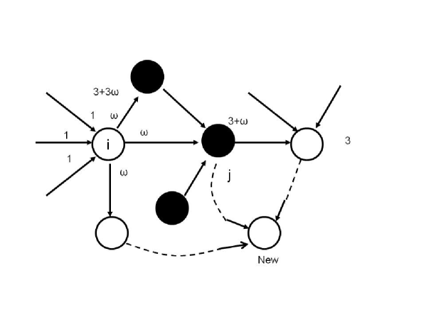
Figure 1: Sample graph with $r=3$. The voter $i$ selects three voters and is selected by three voters. The arrow is from the selected voters to selecting voters. The color is the voting of the voter. The site is white, as he/she voted for candidate $C_{0}$. The popularity of the voter $i$ is $3\omega+3$, and the color is white. The voter $j$ refers three voters and is selected by a voter. He/she is black, as he/she voted for candidate $C_{1}$. The popularity of the site/ the voter $j$ is $3+\omega$, and the color is black.

Samples of the networks are shown in Fig.2. Fig.2 upper side shows the case of $r=1$, which corresponds to tree networks, and the lower side shows the case of $r=3$. We confirmed that this method represents several types of networks.

Next, we discuss the relation between $\omega$ and the hub size. We show that some hubs gather almost all links using Gini coefficient in Fig.3. This is the concentration of links to hubs. Gini coefficient is the index of concentration and shows a number from 0 to 1. As the concentration increased, the Gini coefficient increased. We can confirm that the concentration appears $\omega>0$ and the effect of hubs increases as $\omega$ increases.

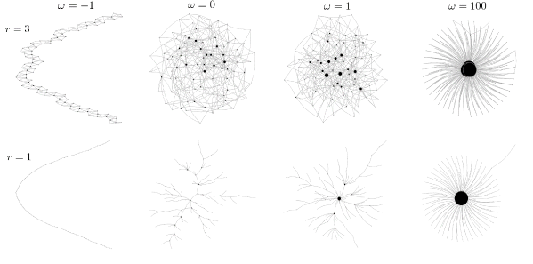
Figure 2: Sample networks with $\omega\in\{-1,0,1,100\}$ in 100 steps. When $r=1$, the network becomes a tree network. When $r=3$, $\omega=1$ corresponds to the BA model. When $\omega>0$, the network is a scale-free network. When $\omega=0$, the network is a random graph. When $\omega=-1$, the network corresponds to an extended lattice.

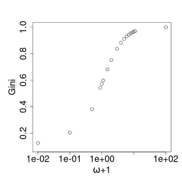
Figure 3: Relation between Gini coefficient and $\omega$. As $\omega$ increases, most of the links would concentrate in certain hubs.

III III. Voting Model

In this section, we introduce the voting model. We model the voting behavior of two candidates, $C_{0}$ and $C_{1}$, at time $t$ and $C_{0}$ and $C_{1}$ have $c_{0}(t)$ and $c_{1}(t)$ votes, respectively. At each time step, one voter votes for one candidate, indicating that voting is sequential. Hence, at time $t$, the $t$-th voter votes, and the total number of votes is $t$. Voters were allowed to view them. $r$ previous votes for each candidate; thus, they are aware of public perception, where $r$ is a constant. The selections made when $r$ previous votes were cast, depending on networks that voters have access to. This is explained in detail in the next section.

In our model, we assume an infinite number of voters of each of the two types: independence and herders. Independent votes for candidates $C_{0}$ and $C_{1}$ have probabilities $1-q$ and $q$, respectively. Their votes are independent of others’ votes; that is, their votes were based on their fundamental values. We assume $q\geq 1/2$. Hereafter, we set $C_{1}$ as the correct candidate, and the ratio voting to candidate $C_{1}$ is the correct ratio used to consider the voting performance.

The herders’ votes were based on the number of previous $r$ votes. Note that the voter does not necessarily refer to the latest $r$ votes. We consider previous $r$ votes to refer to those that were selected from the voters’ network. Therefore, at time $t$, $r$ previous votes are number of votes for $C_{0}$ and $C_{1}$, represented by $c_{0}^{r}(t)$ and $c^{r}_{1}(t)$. Hence, $c_{0}^{r}(t)+c_{1}^{r}(t)=r$ holds. If $r>t$, voters can view $t$ previous votes for each candidate. In the limit $r\rightarrow\infty$, voters can view all previous votes Hisakado3 . We define the number of previous votes for $C_{0}$ and $C_{1}$ as $c_{0}^{\infty}(t)\equiv c_{0}(t)$ and $c_{1}^{\infty}(t)\equiv c_{1}(t)$. In the real world, the number of references $r$ depends on voters; however, we considered $r$ to be constant in this study.

The herder was considered to be a digital herder Hisakado3 . We define $c(t)^{r}_{1}/r=1-c(t)^{r}_{0}/r=Z_{r}(t)$. A digital herder’s behavior is defined by the function $f(z)=\theta(Z_{r}-1/2)$, where $\theta(Z)$ is a Heaviside function, and the threshold was 1/2, corresponding to the majority decision. In W2 , a model in which the threshold was different from 1/2 was discussed. The model corresponds to voting without independent voters.

Independents and herders appear randomly and vote. We set the ratio of independent variables to herders, as $(1-p)/p$. In this study, we focused mainly on the upper limit of $t$, which refers to voting by an infinite number of voters.

IV IV. Voting model on Network

In this section, we combine the network and voting models discussed in the previous two sections. We consider the voter able to view $r$ previous votes. This problem becomes one of determining how voters select $r$ previous votes. In Section II, we define how to select previous voters for reference. The influence of reference voters is represented as a voting model in a network. Our problem lies in how the network affects the voting model. In this study, we analyzed the cases by comparing models based on networks created by a parameter $\omega$. The network includes a random graph, BA model case, and the extended lattice, which correspond to $\omega=1,0,-1$, respectively. In Fig.4, we illustrate each one of these three cases for $r=2$. A white (black) dot indicates a voter who voted for candidate $C_{0}(C_{1})$. The two arrows point toward a dot, indicating that a voter refers to two other voters when $r=2$. In the case of a 1D extended lattice, the voter refers to the latest two voters. In the case of a random graph, a voter refers to two previous voters who were selected randomly. In the case of the BA model, a voter refers to two previous voters selected through the voter’s popularity network. A positive $\omega$ network has the characteristics of a scale-free network with hubs. However, in the negative $\omega$ network, the variance in the number of connections in each node is small.

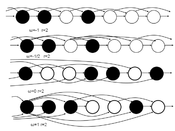
Figure 4: Representation of graphs. An extended 1D lattice, Fermion-like graph, random graph, and BA model, for $\omega=-1,-1/2,0,1$, $r=2$, respectively. The white (black) dot is a voter who voted for the candidate $C_{0}(C_{1})$. Two arrows pointing toward a dot represent a voter who refers to two voters when $r=2$. In the case of an extended 1D lattice, a voter refers to the latest two voters. In the case of a random graph, a voter refers to two previous voters who are selected randomly. In the case of the BA model, a voter refers to two previous voters who are selected via popularity. Hence, there are voters who play the role of a hub in the BA model. The first voter in the network graph is a hub who influences many other voters.

We define $P_{1}^{r}(t)$ as the probability that the $t$th voter would vote for $C_{1}$.

$$P_{1}^{r}(t)=\left\{\begin{array}[]{ll}p+(1-p)q&;c_{1}^{r}(t)>r/2,\\ p/2+(1-p)q&;c_{1}^{r}(t)=r/2,\\ (1-p)q&:c_{1}^{r}(t)<r/2.\end{array}\right\}$$

In the scaling limit, $t=c_{0}(t)+c_{1}(t)=c_{0}^{\infty}+c_{1}^{\infty}\rightarrow\infty$, we define

$$Z(t)=\frac{c_{1}(t)}{t}\Longrightarrow Z_{\infty}.$$ (1)

$Z(t)$ is the ratio of voters who vote for $C_{1}$ at $t$.

Here, we define $\pi(Z)$ as the majority probability of binomial distributions of $Z$, in other words, the probability that $c_{1}^{r}(t)>1/2$. When $r$ is odd,

$$\pi(Z)=\sum_{g=\frac{r+1}{2}}^{r}\left(\begin{array}[]{cc}r\\ g\end{array}\right)Z^{g}(1-Z)^{r-g}.$$ (2)

$\pi$ can be calculated as follows:

$$\pi(Z)=\frac{(2n+1)!}{(n!)^{2}}\int_{0}^{Z}x^{n}(1-x)^{n}dx=\frac{1}{B(n+1,n+1)}\int_{0}^{Z}x^{n}(1-x)^{n}dx.$$ (3)

Eq.(3) can be applied when the referred voters overlap. In fact, the referred voters do not select an overlap. However, in this study, we used this approximation to investigate the large $t$ limit.

Each popularity has a color in the voting model. The color depends on whether the voter voted for candidate $C_{1}$ or $C_{0}$. In Fig.1, voters who voted for $C_{1}$($C_{0}$) are represented by black (white) circles.

We define the total popularity of voters who vote for candidate $C_{1}$($C_{0}$) at $t$ as $g_{1}(t)$($g_{0}(t)$). Thus, $g_{0}(t)+g_{1}(t)=(1+\omega)r(t-r+1)$, where $t\geq r$. In the scaling limit, $g_{0}(t)+g_{1}(t)=(1+\omega)r(t-r+1)\rightarrow\infty$, we define

$$\frac{g_{1}(t)}{(1+\omega)r(t-r+1)}=\hat{Z}(t)\Longrightarrow\hat{Z}_{\infty},$$ (4)

$\hat{Z}(t)$ is $g_{1}(t)/(1+\omega)r(t-r+1)$ at $t$.

We can denote the evolution of popularity as

$$g_{1}(t)=\hat{k}\rightarrow\hat{k}+i:$$

$$r/2\leq j\leq r,i=\omega j+r, P_{\hat{k},t}(i)={}_{r}C_{j}\hat{Z}^{j}(1-\hat{Z})^{r-j}[(1-p)q+p],$$

$$0\leq j<r/2,i=\omega j+r, P_{\hat{k},t}(i)={}_{r}C_{j}\hat{Z}^{j}(1-\hat{Z})^{r-j}(1-p)q,$$

$$r/2\leq j\leq r,i=\omega j, P_{\hat{k},t}(i)={}_{r}C_{j}\hat{Z}^{j}(1-\hat{Z})^{r-j}(1-p)(1-q),$$

$$0\leq j<r/2,i=\omega j, P_{\hat{k},t}(i)={}_{r}C_{j}\hat{Z}^{j}(1-\hat{Z})^{r-j}[(1-p)(1-q)+p].$$

IV.1 A. Information cascade transition

Here, we consider self-consistent equations for popularity at a large $t$ limit.

$$(1+\omega)r\hat{Z}_{\infty}=\sum_{j=1}^{r}P_{\hat{k},t}(i)\cdot i=r(1-p)q+rp\pi(\hat{Z}_{\infty})+r\omega\hat{Z}_{\infty}.$$ (6)

Hence, we can obtain

$$\hat{Z}_{\infty}=(1-p)q+p\pi(\hat{Z}_{\infty}).$$ (7)

This is a self-consistent equation that does not depend on $\omega$. The self-consistent equation for voting ratio $Z_{\infty}$ is also

$$Z_{\infty}=(1-p)q+p\pi(Z_{\infty}).$$ (8)

We define a new variable $\hat{\Delta}_{t}$ such that

$$\hat{\Delta}_{t}=g_{1}(t)-r(t-r+1)=\frac{1}{2}\{g_{1}(t)-g_{0}(t)\}.$$ (9)

For convenience, we changed the notation from $\hat{k}$ to $\hat{\Delta}_{t}$. Therefore, $\hat{\Delta}_{t}$ holds within $\{-r(t-r+1),r(t-r+1)\}$. Given $\hat{\Delta}_{t}=\hat{u}$, we obtain a random walk model:

$$\hat{\Delta}=\hat{u}\rightarrow\hat{u}+i:$$

$$r/2\leq j\leq r,i=(r+(2j-r)\omega/(1+\omega), P_{\hat{u},t}(i)={}_{r}C_{j}\hat{Z}^{j}(1-\hat{Z})^{r-j}[(1-p)q+p],$$

$$0\leq j<r/2,i=(r+(2j-r)\omega/(1+\omega), P_{\hat{u},t}(i)={}_{r}C_{j}\hat{Z}^{j}(1-\hat{Z})^{r-j}(1-p)q,$$

$$r/2\leq j\leq r,i=(r+(2j-r)\omega/(1+\omega), P_{\hat{u},t}(i)={}_{r}C_{j}\hat{Z}^{j}(1-\hat{Z})^{r-j}(1-p)(1-q),$$

$$0\leq j<r/2,i=(r+(2j-r)\omega/(1+\omega), P_{\hat{u},t}(i)={}_{r}C_{j}\hat{Z}^{j}(1-\hat{Z})^{r-j}[(1-p)(1-q)+p],$$

where $\hat{Z}=\hat{k}/(2r(t-r+1))=\hat{u}/(2r(t-r+1))+1/2$.

We now consider the continuous limit $\epsilon\rightarrow 0$

$$\hat{X}_{\tau}=\epsilon\hat{\Delta}_{[\tau/\epsilon]},$$ (11)

where $\tau=t\epsilon$, Approaching the continuous limit, we obtain the following stochastic partial differential equation:

$$\textrm{d}\hat{X}_{\tau} = [\frac{2r(1-p)q}{1+\omega}-\frac{r}{1+\omega}+\frac{\omega}{(1+\omega)}\frac{\hat{X}_{\tau}}{(\tau-r+1)}$$ (12)

$$+\frac{2rp}{1+\omega}\frac{(2n+1)!}{(n!)^{2}}\int_{0}^{\frac{1}{2}+\frac{\hat{X}_{\tau}}{2r(\tau-r+1)}}x^{n}(1-x)^{n}dx]\textrm{d}\tau+\sqrt{\epsilon}\textrm{d}B.$$

For $r=1$, the equation becomes:

$$\textrm{d}\hat{X}_{\tau}=[\frac{(1-p)(2q-1)}{1+\omega}+\frac{p+\omega}{1+\omega}\frac{\hat{X}_{\tau}}{\tau}]\textrm{d}\tau+\sqrt{\epsilon}\textrm{d}B.$$ (13)

The relation between the voting ratio for $C_{1}$ and $\hat{X}_{\infty}$ is

$$\frac{\hat{X}_{\infty}}{2r(\tau-r+1)}=\hat{Z}_{\infty}-\frac{1}{2}.$$ (14)

We can assume that the stationary solution is

$$\hat{X}_{\infty}=r\bar{\hat{v}}\tau+r(1-p)(2q-1)\tau,$$ (15)

where $\bar{\hat{v}}$ denotes a constant. As Eq.(14) and $0\leq\hat{Z}\leq 1$, we obtain

$$-1\leq\bar{\hat{v}}+(1-p)(2q-1)\leq 1.$$ (16)

Substituting Eq.(15) into Eq.(12), we obtain

$$\bar{\hat{v}}=-p+\frac{2p\cdot(2n+1)!}{(n!)^{2}}\int_{0}^{\frac{1}{2}+\frac{(1-p)(2q-1)}{2}+\frac{\bar{\hat{v}}}{2}}x^{n}(1-x)^{n}dx.$$ (17)

This equation is self-consistent equation. Eq.(17) does not depend on parameter $\omega$. Hence, the transition point is the same for all $\omega>-1$.

When $p\leq p_{c}$, the phase is referred to as the peak phase and the solution is $\bar{\hat{v}}_{0}$. Eq.(17) admits three solutions for $p>p_{c}$: When $p>p_{c}$, the upper and lower solutions are are stable; on the contrary, the intermediate solution is unstable. The two stable solutions correspond to good $\bar{\hat{v}}_{+}$ and bad equilibria $\bar{\hat{v}}_{-}$, respectively, and the distribution becomes the sum of two Dirac measures. This was a two-peak phase.

The phase transition point, $p_{c}$ is common for all models. If $r=2n+1\geq 3$, then a phase transition occurs in the range $0\leq p\leq 1$. If a voter obtains information from either one or two voters, there is no phase transition.

IV.2 B. super-normal transition

We expand $\hat{X}_{\tau}$ around solution $\bar{\nu}=r\bar{\hat{v}}\tau+r(1-p)(2q-1)\tau$.

$$\hat{X}_{\tau}=r\bar{\hat{v}}\tau+r(1-p)(2q-1)\tau+r\hat{W}_{\tau}.$$ (18)

We set $\hat{X}_{\tau}\gg\hat{W}_{\tau}$. This result indicates that $\tau\gg 1$. We rewrite Eq.(12), using Eq.(18) and obtain the following:

$$\textrm{d}\hat{W}_{\tau} = [\frac{\omega+pA}{1+\omega}]\frac{\hat{W}_{\tau}}{\tau}\textrm{d}\tau+\sqrt{\epsilon}\textrm{d}B,$$ (19)

where

$$A=\frac{(2n+1)!}{(n!)^{2}\cdot 2^{2n}}(1-\{\bar{\hat{v}}+(1-p)(2q-1)\}^{2})^{n}.$$ (20)

The trend in this solution is $(\omega+pA)/(1+\omega)$ where: there is a transition in the trend at the $(\omega+pA)/(1+\omega)=1/2$. We set the solution to this equation as $p_{vc}$. When $(\omega+pA)/(1+\omega)>1/2$, the convergence speed is slower than that in the normal case. However, when $(\omega+pA)/(1+\omega)<1/2$, the convergence speed is slower than in the normal case. We call this transition a super-normal transition, and the transition point is $p_{vc}$.

When $\omega\geq 1$, $(\omega+pA)/(1+\omega)\geq 1/2$ because $A\geq 0$. Thus, there is no super-normal transition at $\omega\geq 1$. We observed a super-normal transition at $1>\omega>-1$.

IV.3 C. Symmetric case, $q=1/2$

Here, we consider a symmetric model $q=1/2$. When $r\geq 3$, there are two stable solutions and one unstable solution $\bar{\hat{v}}=0$ above $p_{c}$. The vote ratio for $C_{1}$ is a good or bad equilibrium. In one sequence, $Z$ is taken as $\bar{\hat{v}}/2+1/2$ in the case of good equilibrium or as $-\bar{\hat{v}}/2+1/2$ in the case of bad equilibrium. where $\bar{\hat{v}}$ is the solution of Eq.(17). This indicates a two-peak phase and critical point is $p_{c}=\frac{(n!)^{2}}{(2n+1)!}2^{2n}=1/A$, where the gradient of the RHS of Eq.(17) at $\bar{\hat{v}}=0$ is $1$. In the case of $r=3(n=1)$, $p_{c}=2/3$ and $r=5(n=2)$, $p_{c}=8/15$. As $r$ increases, $p_{c}$ moves toward $0$. In the large limit, $r\rightarrow\infty$, $p_{c}$ becomes $0$. This is consistent with the case where herders obtain information from all previous voters Hisakado3 . The discussion above does not depend on $\omega$. In the limit $\omega=-1$, there is no phase transition in the lattice case.

We consider the super-normal transition in the symmetric case $q=1/2$ by considering the case $r=2n+1\geq 3$. In this case, we observe an information cascade transition. If $r\leq 2$, an information cascade transition is not observed.

In one-peak phase $p\leq p_{c}$, the only solution is $\bar{\hat{v}}=0$. $p_{c}$ is the critical point of information cascade transition. The critical point of the convergence is $p_{vc}=(1-\omega)/2A=\frac{(1-\omega)}{2}p_{c}$.

Above $p_{c}$, in the two-peak phase, we obtain two stable solutions that are not $\bar{\hat{v}}=0$. At $p_{c}$, $\bar{\hat{v}}$ moves from $0$ to one of two stable solutions. In one voting sequence, votes converge to one of these stable solutions. Here, $\bar{\hat{v}}$ is the solution of Eq.(17). In the case $r=3$ we obtain $\bar{\hat{v}}=\pm\sqrt{(3p-2)/p}$ and $p_{c}=2/3$. The critical point of convergence in the two-peak phase was $p_{vc}=(5+\omega)/6$.

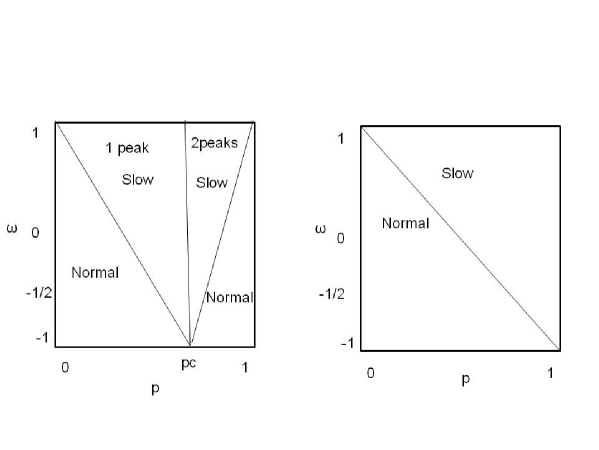
Figure 5: Phase diagram of the symmetric case ($q=1/2)$ for $r=1$ and $r=3$ cases. In the case of $r=3$, $p_{c}$ is 2/3. The horizontal axis is $p$, and the vertical axis is $\omega$.

In Fig.5. we show the phase diagrams for the cases $q=1/2$, $r=3$, and $r=1$. In the case $r=1$, there is only a super-normal transition. The super-normal transition disappeared at $\omega=-1$. In the case $r=3$ we can confirm two types of phase transitions, the information cascade transition and a super-normal transition. The super-normal transition disappeared at $\omega=-1$. In the analog herder case, the phase diagram becomes the same as in the $r=1$ case. Analog herders vote for each candidate with probabilities proportional to the candidates’ votes.

IV.4 D. Asymmetric case, $q\neq 1/2$

Next, we consider the asymmetric case. In this case, the phase transition is of the first kind that exhibits a discontinuity at the critical point $p_{c}$. We investigated the correct ratio for this phase transition. To define the correct ratio, we assume that candidate 1(0) is the correct(wrong) one. The correct ratio of independent voters is $q>1/2$, and the correct ratio of the herder determines the total correct ratio. Using the correct ratio, we can confirm the voting performance. The phase transition has a negative effect on this performance. In Fig.6, we show the image of the correct ratio in several $\omega$. The horizontal axis represents $p$ and the vertical axis represents the correct ratio. We observe a gap in the correct ratio at the the transition point $p_{c}$ when $\omega>-1$ $p_{c}$ does not depend on $\omega$. When $\omega=-1$, no phase transition occurred.

In the limit $\omega\rightarrow\infty$, the trend of Eq.(19) is 1 for all $Z$. In this case, the hubs have the maximum links. At the critical point $p_{c}$ the correct ratio depends only on the initial voting. The two equilibria are $\bar{\hat{v}}_{+}$ and $\bar{\hat{v}}_{-}$. The probabilities of good and bad equilibria are $\alpha$ and $\beta$. The correct ratio was $Z_{\infty}=(\alpha\bar{\hat{v}}_{+}+\beta\bar{\hat{v}}_{-})/2+1$. In the case $\omega\rightarrow\infty$, we obtain $Z_{\infty}=(\alpha\bar{\hat{v}}_{+}+\beta\bar{\hat{v}}_{-})/2+1=p/2+(1-p)q$, which is the dotted bottom line in Fig.6. In this case, we could not obtain the effects of herders. In general, for $\omega>-1$, we obtain

$$\lim_{p\rightarrow p_{c}}\bar{v}=2\bar{\hat{v}}-1>(\alpha\bar{\hat{v}}_{+}+\beta\bar{\hat{v}}_{-})/2+1\geq p/2+(1-p)q.$$ (21)

In summary, in the one-peak phase, the correct ratio did not depend on $\omega$. On the contrary, in the two-peak phase, the correct ratio depends on $\omega$, which is the network. As $\omega$ increased, the gap at the transition points increases and the correct ratio decreases. In other words, the correct ratio of the herders decreases. In the lattice case $\omega=-1$, there is no phase transition, and the correct ratio increases without the phase transition as $p$ increases. The lattice case is summarized in Appendix C. The effects of the hubs were observed in the correct ratio during the two-peak phase. As the hub effects increased, the gap increased.

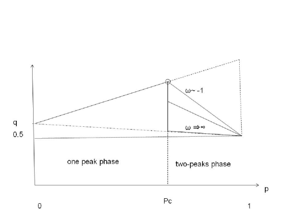
Figure 6: Expected correct ratio and first kind phase transition for the asymmetric case. The effects of the hubs are observed in the correct ratio in the two-peak phase. As the effects of the hub increases, the gap increases.

V V. Numerical Study of Phase Transitions

In this section, we present the results of the numerical studies on phase transitions of the voting model in the networks. We adopted the model parameters $(r,q)$ as $r=3$ and $q\in\{0.5,0.6\}$ and change the control parameter $p\in[0,1]$. With regard to $\omega$, we adopt $\omega\in\{-0.9,-2/3,-1/2,0,1,2,9\}$. We estimate the statistical quantities of the model using a simple Monte Carlo sampling. Using the probabilistic rule of the network, voting model, we generated $10^{2}$ networks and $10^{4}$ sample sequences in each network. After estimating the statistical quantities by taking the average over the sample sequences, we calculated the average of the networks. To estimate the universal function of a continuous transition, we generated $10^{4}$ and $10^{4}$ sample sequences.

When $\omega=-1$, we adopt an extended lattice with $r=3$, which is different from that of the network with $\omega=-1$ because of the initial condition of the network. We used a perfect network as the initial condition for this numerical simulation.

Probability that voter 1 was chosen by the next voters.is zero, because the the in-degrees is 0. In addition, the in-degrees and popularity of Voters 2 and 3 are 1 and 2, respectively. Because they are smaller than those of the voters for $t>3$, they are chosen less by the next voters.

V.1 A. Symmetric case, $q=1/2$

In this subsection, we consider the symmetric case, $q=1/2$. A phase transition occurred at $p=p_{c}=2/3$. In the one-peak phase $p<p_{c}=2/3$, $Z(t)$ converges to the unique solution to Eq. (8). There is also a super-normal transition at $p=p_{vc}=(1-\omega)/3$. The power-law exponent $\gamma$ of $V(Z(t))\propto t^{-\gamma}$ is given by

$$\gamma=\left\{\begin{array}[]{cc}1&p<p_{vc},\\ (2-3p)/(1+\omega)&p>p_{vc},\end{array}\right.$$

where $V(Z(t))$ is the variance of $Z(t)$. Here, $\gamma=1$ is the normal phase and $0<\gamma<1$ is the super diffusion phase. We estimate $\gamma$ using the following estimator: $\hat{\gamma}=\log_{2}V(Z(T/2))/V(Z(T))$,

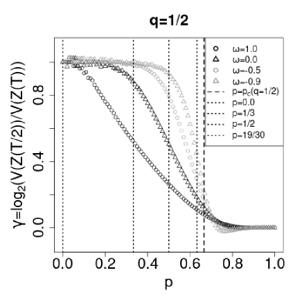
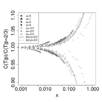
Figure 7: Left: Plot $\gamma$ vs. $p$ for $q=0.5,r=3$ and $T=10^{4}$. $\omega=1(\mbox{black}\bigcirc),0.0(\mbox{black}\bigtriangleup),-0.5(\mbox{gray}\circ)$ and $-0.9(\mbox{gray}\bigtriangleup)$. The broken and dotted lines show the value of $p_{c}=2/3$ and $p_{vc}(q,\omega)$ for $\omega\in\{1,0.0,-0.5,-0.9\}$. Right: Plot of the universal function and the estimated ones. For $\omega\in\{0(\mbox{black}\bigcirc),1(\mbox{black}\bigtriangleup),2(\mbox{black}+),9(\mbox{black}\times),-0.5(\mbox{gray}\bigcirc),-2/3(\mbox{gray}\bigtriangleup),-0.9(\mbox{gray}+)\}$ we plot $C(T|p)/C(T|p_{c})$ as function of $x$ in eq.(22). The gray lines show the universal function $g(x)$ of Eq.(22) for $p>p_{c}$(gray solid) and $p<p_{c}$(gray broken).

The left figure of Fig.7 plots $\gamma$ vs. $p$ for $\omega\in\{1,0,-0.5,-0.9\}$. The horizontal axis represents the ratio of herders $p$. The vertical axis represents the speed of convergence $\gamma$. The vertical broken line indicates the critical point, $p_{c}(1/2)=2/3$. The other vertical dotted lines show $p_{vc}$ for $\omega\in\{1,0,-0.5,-0.9\}$, respectively. The phase transition occurs at $p=p_{c}(1/2)$. For $p>p_{c}$, $\gamma$ is almost zero and the variance in $Z(t)$ becomes constant. There are two stable states. For $p>p_{c}$, $V(Z(t))$ does not decrease to zero. For $p<p_{c}$, a super-normal transition occurs. The positions of the critical points are vague; evidently, the region $p$ for the normal phase for $\omega=1$ is extremely narrow, and it considers $p_{vc}(\omega=1)=0$. For $\omega=0$, $p_{vc}=1/3$ and a plateau region was observed for $p<0.25$. As $\omega$ decreases from $\omega=1\to-0.9$, the plateau region widens. Near the critical point $p_{vc}$, $\gamma$ is smaller than one, and estimating $p_{vc}$ from the figure is difficult.

To study the universality class of continuous phase transitions at $p_{c}$, we examined the order parameter $C(T)$. $C(T)$ is defined as follows.

$$C(t|p)=E(c_{1}(t+1)|c_{1}(1)=1)-E(c_{1}(t+1)|c_{1}(1)=0),$$

and reflects the sensitivity of the initial condition for the stochastic process.

In Fig.8, we show the critical exponent $\alpha=1/2$ and it does not depend on $\omega$.

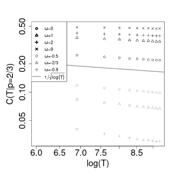
Figure 8: Plot $C(T)$ vs Log $T$ at $\omega=9,2,1,0,-0.5,-2/3,-0.9$. $\alpha=1/2$ and does not depend on $\omega$.

As discussed in Appendix B, the universal function $g(x)$ of the continuous phase transition for the symmetric case is defined as

$$g(x)=\lim_{t\to\infty}C(t|p)/C(t|p_{c})=\left\{\begin{array}[]{cc}\sqrt{\frac{x}{1-e^{-x}}}&p\to p_{c}-0,t\to\infty,x=\frac{3(p_{c}-p)/2}{1+\omega}\ln t,\\ \sqrt{\frac{2x}{e^{2x}-1}}&p\to p_{c}+0,t\to\infty,x=\frac{3(p-p_{c})}{1+\omega}\ln t.\\ \end{array}\right.$$ (22)

V.2 B. Asymmetric case, $q=0.6$

A phase transition occurred at $p=p_{c}(q=0.6)=0.781$. As in the symmetric case $Z(t)$ converges to the unique solution to Eq.(8) for one-peak phases for $p<p_{c}$. The variances of $Z(t)$ and $V(Z(t))$ also decrease to zero in the limit. There is also a super-normal transition at $p=p_{vc}(0.6)$. When $\omega=1(0)$, $p_{vc}=0(0.360)$. When $\omega=-0.5,-0.9$, only the normal convergence phase exists.

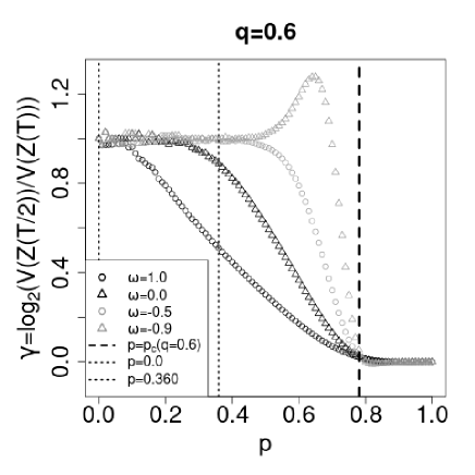
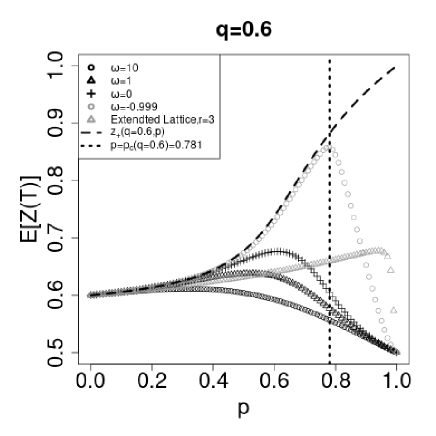
Figure 9: Plot $\gamma$ vs. $p$ for $q=0.6,r=3$ and $T=10^{4}$. $\omega=1(\mbox{black}\circ),0.0(\mbox{black}\bigtriangleup),-0.5(\mbox{gray}\circ)$ and $-0.9(\mbox{gray}\bigtriangledown)$. The broken solid and dotted lines show the value of $p_{c}(q=0.6)=0.781$ and $p_{vc}(q=0.6,\omega)$ for $\omega\in\{1,0.0\}$. The is no super-phase for $\omega\in\{-0.5,-0.9\}$. Right: Plot of the $z_{+}(q=0.6,p)$, the unique solution of Eq.(7) for $p<p_{c}$ and the larger solution of Eq.(7) for $p>p_{c}$ and the estimated expected value of $Z(T)$ vs. $p$. $\omega=10(\mbox{black}\bigcirc),1(\mbox{black}\bigtriangleup),0(\mbox{black}+),-0.999(\mbox{gray}\bigcirc)$ and the extended lattice $(gray\bigtriangledown)$. The thin dotted line shows $p=p_{c}(0.6)$.

The left figure of Fig.9 plots $\gamma$ vs. $p$ for $\omega\in\{1,0,-0.5,-0.9\}$. The horizontal axis represents the ratio of herders $p$. The vertical axis represents the speed of convergence $\gamma$. The vertical broken line indicates the critical point, $p_{c}(q=0.6)$. The other vertical dotted lines show $p_{vc}$ for $\omega\in\{1,0\}$, respectively. It is clear that the phase transition at $p=p_{c}(q=0.6)$. For $p>p_{c}$, $\gamma$ is almost zero and the variance in $Z(t)$ becomes constant. There are two stable states. For $p>p_{c}$, $V(Z(t))$ does not decrease to zero. For $p<p_{c}$, a super-normal transition occurs. The positions of the critical points are vague; evidently, the region $p$ for the normal phase for $\omega=1$ is extremely narrow, and it considers $p_{vc}(\omega=1)=0$. For $\omega=0$, $p_{vc}\simeq 0.36$ and a plateau region was observed for $p<0.3$. As $\omega$ decreases from $\omega=1\to-0.9$, the plateau region widens. Near the critical point $p_{vc}$, $\gamma$ is smaller than one, and estimating $p_{vc}$ from the figure is difficult.

In the asymmetric case, the phase transition at $p_{c}(q),q>1/2$ is discontinuous. The image on the right side of Fig.9 shows the average value of $Z(T)$, which is the correct value. In addition to this network model, $\omega\in\{10,1,0,-0.999\}$, we show the results for extended lattice case. As there is only one stable state for $p<p_{c}(q)$, $Z(t)$ converges to the solution to Eq.(8). We denote this solution as $z_{+}(q,p)$ in Fig.10. The figure shows that the convergence speed crucially depends on $\omega$. When $\omega=10$ and $T=10^{4}$, as $p$ increases from 0 to 1, the average value of $Z(T)$ deviates from $z_{+}(q=0.6,p)$. As $\omega$ decreases to -1, the departure timing is delayed, and at $\omega=-0.999$, the average value coincided with $z_{+}(q,p)$ until $p_{c}(q)$. For $p\geq p_{c}$, there are two stable solutions to Eq.(8), and we denote them as $z_{+}(q,p)=2\bar{\hat{v}}_{+}-1$ and $z_{-}(q,p)=2\bar{\hat{v}}_{-}-1$. $z_{+}(q,p)$ is a larger solution, and the unique solution for $p<p_{c}(q)$ continuously becomes $z_{+}(q,p)$ for $p>p_{c}(q)$. In the case $p<p_{c}(q)$, the expected value is the weighted average of $z_{+}(q,p)$ and $z_{-}(q,p)$. In the limit $T\to\infty$, $E(Z(T))$ converged to $z_{+}(q,p)$. The results suggest that the discontinuity in $E(Z(T))$ in the limit $T\to\infty$ at $p=p_{c}$ depends on $\omega$.

From the viewpoint of the performance, network $\omega\sim-1$ exhibits the best performance among all networks. There was a phase transition; however, the gap was small. Hence, the highest correct ratio can be confirmed for $\omega\geq-1$. However, when there is a large hub, the gap becomes large and the performance worsens in the two-peak phase. When the lattice case ${}^{\omega}=-1$, there is no phase transition; however, the performance is worse than the other networks.

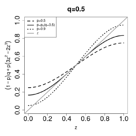
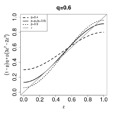
Figure 10: Solutions of Eq.(8) for the case $r=3$ and $q=0.5,0.6$. The left figure is the symmetric case and the right figure is the asymmetric case. The horizontal axis is $Z$, and the vertical axis is the RHS of Eq.(8). In both figure when $p<p_{c}$, there is only one solution. When $p>p_{c}$, there are three solutions. The right solutions are $z_{+}$ and the left solutions are $z_{-}$. $z_{+}$ and $z_{-}$ are the stable solutions.

VI VI. Concluding Remarks

In this study, we examined a voting model by considering several different types of networks, including a random graph, the Barabási–Albert(BA) model, and lattice networks, using one parameter $\omega$. For a positive $\omega$, the network has hubs. However, for negative $\omega$, the network has a limit on the number of links. Using $\omega$, we continuously studied the effects of network.

We investigated the phase differences between different networks as models for the source of voter information. This is based on the assumption that voters obtain information from a network, including hubs. A voting model represents how public perceptions are conveyed to voters. Our voting model was constructed using two types of voters—herders and independents—and two candidates. Herders vote for the majority of candidates and obtain information related to previous votes from their networks. We examined the differences between the phases on which networks depend.

In $\omega>-1$, we observed two types of phase transition: cascade transition, and super-normal transition. As the number of herders increased, the model featured a phase transition beyond which a state in which most voters made the correct choice coexisted with one in which most of them were wrong. During this transition, the distribution of votes changed from the one-peak phase to the two-peak phase. The other transition is a super-normal transition in terms of convergence speed.

In the symmetric case information cascade transition is continuous. transition. However, in the asymmetric case, it was discontinuous. We confirmed that the transition point of the information cascade transition does not depend on $\omega$ for both the symmetric and asymmetric cases. In the symmetric case, information cascade transition does not depend on the network. However, in the asymmetric case, the gap in the discontinuous phase transition depends on the network. As $\omega$ increased, the gap increased. In other words, the hubs affect the phase transition gap. In the two-peak phase, hubs affect the correct ratio. However, in the one-peak phase, the hubs do not affect the correct ratio. The super-normal transition also depends on the network. As $\omega$ increases, transition point $p_{c}$ decreases. At $\omega=1$, the transition disappears, and at $\omega\geq 1$, convergence is slow for any $p$. Hence, a phase transition was observed in $1>\omega>-1$. This is the same as the percolation model for the network, which we show in Appendix D. This is effective for both the symmetric and asymmetric cases.

For $\omega=-1$ which belongs to the lattice network, there was no phase transition. Hence, the correct ratio increased as $p$ increased because there is no phase transition. The lattice case is summarized in Appendix C.

In Table 1 we summarize the relations between the networks and information cascade transition. In this study, we considered the networks corresponding to $\omega\neq-1$ the lattice with $\omega=-1$. In the lattice case there was no phase transition Hisakado4 . By contrast, in networks with $\omega\neq-1$, a phase transition occurred. In the symmetric case, it is a continuous transition with critical exponent $\beta=1/2$. The universality class is the same as that of the nonlinear Pólya model Hill ; Pem1 ; Pem2 . This is an absorption transition that belongs to the non-equilibrium phase transition Hin ; Lu . In the asymmetric case, the transition is discontinuous. When all voters are refereed, the model belongs to universality class of the voter model. In this case, the critical exponent is $\beta=1$ and it belongs to the universality class of the voter model Hin ; Lu .

Table 1: Networks and the universality class in the voting model

Model	All $r=t$	Networks $\omega\neq-1$	Lattice $\omega=-1$
Symmetry	$\beta=1$mori2	$\beta=1/2$ mori1 ; mori3	Oscillation Hisakado4
Asymmetry	$\beta=1$ mori2	first kind phase transition	Oscillation Hisakado4

Appendix G Appendix A. Relation to Elephant Walk

In this Appendix, we consider the relationship between voting model used in this study and the elephants walk over a network ele . In the random graph case, and $r=1$ the model corresponds to standard elephant work. Here, the number of referred voters was $r$. Network effects are the differences between the memories. This old behavior is referred to as $\omega$ increases, the old behavior is referred.

Here, we set $p=1$ and consider the case where all voters are herders in the voting model. We use $\hat{p}$ as the parameter instead of $p$ in the voting model. We define $P_{1}^{r}(t)$ as the probability that the $t$th voter would vote for $C_{1}$. We change Eq.   (IV) to

$$P_{1}^{r}(t)=\left\{\begin{array}[]{ll}\hat{p}&:c_{1}^{r}(t)>r/2,\\ \hat{p}/2&;c_{1}^{r}(t)=r/2,\\ (1-\hat{p})&:c_{1}^{r}(t)<r/2.\end{array}\right\}$$

With probability $\hat{p}$, the voter decides based on the referred voters. That is, the difference between $p$ and $\hat{p}$ is the introduction of noise. In the voting model, the voter behaves as herder. In other words, the voter behaves in accordance with the information obtained. By contrast, in the elephant walk model, the voter behaves against the referred information with probability $1-\hat{p}$. In the case $\hat{p}<1/2$, the probability that the voter behaves against the referred information is larger than the voter behaves according to the obtained information. In the case $r=1$, the model becomes an elephant walk model. When the analog herder case corresponds to the elephant model, the phase diagram becomes the same as that of the $r=1$ digital herder case. A voter refers to only one of the previous voters. Analog herders vote for each candidate with probabilities proportional to the candidates’ votes. The initial condition of the elephant model is $P_{1}^{r}(1)=\hat{q}$ and includes an asymmetric case. Here, we consider the symmetric case, $\hat{q}=1/2$.

We can write the evolution of connectivity as

$$g_{1}(t)=\hat{k}\rightarrow\hat{k}+i:$$

$$r/2\leq j\leq r,i=\omega j+r P_{\hat{k},t}(i)={}_{r}C_{j}\hat{Z}^{j}(1-\hat{Z})^{r-j}\hat{p},$$

$$0\leq j<r/2,i=\omega j+r P_{\hat{k},t}(i)={}_{r}C_{j}\hat{Z}^{j}(1-\hat{Z})^{r-j}(1-\hat{p}),$$

$$r/2\leq j\leq r,i=\omega j P_{\hat{k},t}(i)={}_{r}C_{j}\hat{Z}^{j}(1-\hat{Z})^{r-j}(1-\hat{p}),$$

$$0\leq j<r/2,i=\omega j P_{\hat{k},t}(i)={}_{r}C_{j}\hat{Z}^{j}(1-\hat{Z})^{r-j}\hat{p},$$

Approaching the continuous limit, as in Section IV, we can obtain the stochastic partial differential equation:

$$\textrm{d}\hat{X}_{\tau} = [\frac{\omega}{(1+\omega)}\frac{\hat{X}_{\tau}}{(\tau-r+1)}$$ (24)

$$+\frac{r(2p-1)}{1+\omega}\{\frac{2\cdot(2n+1)!}{(n!)^{2}}\int_{0}^{\frac{1}{2}+\frac{\hat{X}_{\tau}}{2r(\tau-r+1)}}x^{n}(1-x)^{n}dx-1\}]\textrm{d}\tau+\sqrt{\epsilon}.$$

When we set $2\hat{p}-1=p$, Eq.(24) becomes Eq.(12).

For $r=1$, the equation becomes

$$\textrm{d}\hat{X}_{\tau}=[\frac{2p-1+\omega}{1+\omega}\frac{\hat{X}_{\tau}}{\tau}]\textrm{d}\tau+\sqrt{\epsilon}.$$ (25)

We can assume that the stationary solution is

$$\hat{X}_{\infty}=r\bar{\hat{v}}\tau+r(1-p)(2q-1)\tau,$$ (26)

where $\bar{\hat{v}}$ denotes a constant. As Eq.(14) and $0\leq\hat{Z}\leq 1$, we obtain

$$-1\leq\bar{\hat{v}}+(1-p)(2q-1)\leq 1.$$ (27)

Substituting Eq.(26) into Eq.(24), we obtain

$$\bar{\hat{v}}=(2p-1)\{\frac{2\cdot(2n+1)!}{(n!)^{2}}\int_{0}^{\frac{1}{2}+\frac{\bar{\hat{v}}}{2}}x^{n}(1-x)^{n}dx-1\}.$$ (28)

This equation is self-consistent. The equation does not depend on parameter $\omega$.

We expand $\hat{X}_{\tau}$ around solution $r\bar{\hat{v}}\tau+r(1-p)(2q-1)\tau$.

$$X_{\tau}=r\bar{\hat{v}}\tau+r\hat{W}_{\tau}.$$ (29)

We set $X_{\tau}\gg W_{\tau}$. This result indicates that $\tau\gg 1$. We rewrite Eq.(24), using Eq.(29), and obtain the following:

$$\textrm{d}\hat{W}_{\tau} = [\frac{\omega+(2p-1)A}{1+\omega}]\frac{W_{\tau}}{\tau}\textrm{d}\tau+\sqrt{\epsilon},$$ (30)

where

$$A=\frac{(2n+1)!}{(n!)^{2}\cdot 2^{2n}}(1-\bar{\hat{v}}^{2})^{n}.$$ (31)

The phase diagram of the elephant walk is shown in Fig.11. We can map from Fig.11 to Fig.5 if we set $2\hat{p}-1=p$. The case $r=1$ corresponds to the elephant walk. We can confirm a super-normal transition. of the basic elephant work model at $\hat{p}=3/4$ ele .

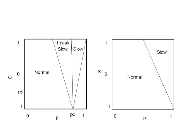
Figure 11: Phase diagram of elephant walk for $r=1$ and $r=3$ cases for the symmetric case $q=1/2$. In the case $r=3$, $p_{c}$ is 2/3.

Appendix H Appendix B. Universal Function for Symmetric Model

In this section, we describe the calculation of the universal function for the symmetric case mori1 ; mori2 ; mori3 . Here, we consider correlation function $C(t)$. The asymptotic behavior $C(t)$ is described by the scaling form for the symmetric case as

$$C(t)\propto(\ln t)^{-1/2}g(\ln t/\xi),$$ (32)

where $g(x)$ is the universal fun cation and $\xi$ denotes the correlation length mori1 ; mori2 . $\xi$ characterizes length scale of the correlation function $C(t)\propto e^{-t/\xi}$.

We used the new random variable $\hat{Y}_{\tau}=\hat{X}_{\tau}/(\tau-r+1)$. Eq.(12).

$$d\hat{Y}_{\tau}=\frac{\varphi(\hat{Y}_{\tau})}{\tau-r+1}d\tau+\frac{\sqrt{\varepsilon}}{\tau-r+1}dB,$$ (33)

where

$$\varphi(y) = f(y)-y=\frac{2r}{1+\omega}\left\{(1-p)(q-1/2)-\frac{y}{2r}+p\rho\left(\frac{y}{2r}\right)\right\},$$

$$\rho(z) = \pi\left(z+\frac{1}{2}\right)-\frac{1}{2}.$$ (34)

$\pi(z)$ is the regularized beta function $I_{z}(n+1,n+1)$ HB . The important property of function $\rho(z)$ is that it is a $\tanh$-shaped function, such that

$$\rho\left(\pm\frac{1}{2}\right) = \pm\frac{1}{2},\quad\rho(z)+\rho(-z)=0,$$

$$\rho^{\prime}(z) = \frac{1}{p_{0}}(1-4z^{2})^{n},\quad p_{0}\equiv\frac{(2n)!!}{(2n+1)!!}.$$ (35)

When $p\leq p_{0}$, function $\varphi(y)$ has only one zero within the range $-r\leq y\leq r$. However, when $p>p_{0}$, three distinct zeros for a sufficiently small $q$ in the same interval. In particular, for the $q=1/2$ case, function $\varphi(y)$ recovers $Z_{2}$symmetry, $\varphi(-y)=-\varphi(y)$. Thus, the system exhibits a continuous phase transition at critical point $p=p_{c}$ where $p_{c}=p_{0}$.

We perturbatively solve Eq.(33) under the initial condition: $\hat{Y}_{\tau}=Y_{0}$ and We expand the random variable $\hat{Y}_{\tau}$ to powers of $\sqrt{\varepsilon}$,

$$\hat{Y}_{\tau}=\hat{Y}_{\tau}^{(0)}+\sqrt{\varepsilon}\hat{Y}_{\tau}^{(1)}+(\sqrt{\varepsilon})^{2}\hat{Y}_{\tau}^{(2)}+\cdots,$$ (36)

and Eq.   (33) is solved recursively. First, the classical solution $\hat{Y}_{\tau}$ is given by

$$\int_{Y_{0}}^{\hat{Y}_{\tau}^{(0)}}\!\frac{dy}{\varphi(y)}=\log(\tau-r+1).$$ (37)

Then, $\hat{Y}_{\tau}^{(1)}$ and $\hat{Y}_{\tau}^{(2)}$ can be expressed as

$$\hat{Y}_{\tau}^{(1)} = \varphi(\hat{Y}_{\tau}^{(0)})\!\int_{r}^{\tau}\!\frac{dB_{s}}{\varphi(\hat{Y}_{s}^{(0)})(s-r+1)},$$

$$\hat{Y}_{\tau}^{(2)} = \frac{\varphi(\hat{Y}_{\tau}^{(0)})}{2}\int_{r}^{\tau}\!\frac{\varphi^{\prime\prime}(\hat{Y}_{s}^{(0)})(\hat{Y}_{s}^{(1)})^{2}}{\varphi(\hat{Y}_{s}^{(0)})(s-r+1)}\,ds.$$ (38)

Notably, the expectation values are given by

$$\mathrm{E}[\hat{Y}_{\tau}^{(1)}] = 0,$$ (39)

$$\mathrm{E}[(\hat{Y}_{\tau}^{(1)})^{2}] = \varphi(\hat{Y}_{\tau}^{(0)})^{2}\int_{r}^{\tau}\!\frac{ds}{\varphi(\hat{Y}_{s}^{(0)})^{2}(s-r+1)^{2}},$$ (40)

$$\mathrm{E}[\hat{Y}_{\tau}^{(2)}] = \frac{\varphi(\hat{Y}_{\tau}^{(0)})}{2}\int_{r}^{\tau}\!\frac{\varphi^{\prime\prime}(\hat{Y}_{s}^{(0)})E[(\hat{Y}_{s}^{(1)})^{2}]}{\varphi(\hat{Y}_{s}^{(0)})(s-r+1)}\,ds.$$ (41)

Let $Y^{\pm}_{\tau}$ denote the solution to Eq.(33) with the initial conditions $Y_{0}=\pm r$. Subsequently, the autocorrelation function is given by

$$C_{X}(\tau)=c\left\{\mathrm{E}[\hat{Y}_{\tau}^{+}+\varphi(\hat{Y}_{\tau}^{+})]-\mathrm{E}[\hat{Y}_{\tau}^{-}+\varphi(\hat{Y}_{\tau}^{-})]\right\},$$ (42)

where $c$ denotes a constant. As seen from Eq.(39), the long-term behavior of $C_{X}(\tau)$ is governed by the classical solution $Y^{(0)\pm}(\tau)$ because $Y^{(0)\pm}(\tau)$ converges to zero for $\varphi(y)$, Thus, we have

$$C_{X}(\tau)\sim\frac{c\omega}{1+\omega}(Y^{(0)+}(\tau)-Y^{(0)-}(\tau))+O((\sqrt{\varepsilon})^{2}).$$ (43)

Now, we concentrate on the $q=1/2$ symmetric model, $p\sim p_{c}$, and $\tau\sim\infty$ case. Subsequently, the classical solution reads as follows:

$$Y^{(0)\pm}(\tau)\simeq\pm c^{\prime}\sqrt{\frac{p^{\prime}}{1-(1-4p^{\prime})(\tau-r+1)^{2\varphi^{\prime}(0)}}},$$ (44)

where

$$p^{\prime}=\frac{3r^{2}((p_{c}/p)-1)}{n}.$$ (45)

Therefore, we obtain the universal function:

$$g(x)=\lim_{\tau\rightarrow\infty}\frac{C_{X}(\tau|p)}{C_{X}(\tau|p_{c})}=\left\{\begin{array}[]{@{\,}ll}\sqrt{\frac{x}{1-e^{-x}}},&x=\frac{2(p/p_{c}-1)}{1+\omega}\log\tau,\quad p\rightarrow p_{c}+0,\\ \sqrt{\frac{2x}{e^{2x}-1}},&x=\frac{1-p/p_{c}}{1+\omega}\log\tau,\quad p\rightarrow p_{c}-0.\end{array}\right.$$ (46)

Appendix I Appendix C. Lattice Case

In this section, we summarize the extended lattice case Hisakado4 . Here, we consider a random walk between the two states $c_{1}^{r}(t)/r>1/2$ (good equilibrium) and $c_{0}^{r}(t)/r>1/2$ (bad equilibrium). We define the hopping probability from state $c_{0}^{r}(t)/r>1/2$ to $c_{1}^{r}(t)/r>1/2$ as $a$ and that from the state $c_{1}^{r}(t)/r>1/2$ to $c_{0}^{r}(t)/r>1/2$ as $b$. $a$ and $b$ are not functions of $t$. When $t>r$, the transition matrix $\hat{A}$ of the random walk is

$$\hat{A}=\left(\begin{array}[]{ll}1-a&a\\ b&1-b\end{array}\right).$$

The random walk of the two states is defined as transition matrix $\hat{A}$ when $t>r$. If $r>t$, voters can view $t$ previous votes for each candidate.

If consecutive independent voters choose candidate $C_{1}(C_{0})$ when $c_{0}^{r}(t)/r>1/2(c_{1}^{r}(t)/r>1/2)$, the state changes from $c_{0}^{r}(t)/r>1/2(c_{1}^{r}(t)/r>1/2)$ to $c_{1}^{r}(t)/r>1/2(c_{0}^{r}(t)/r>1/2)$. Thus, independent voters act as switches for hopping. When independent voters who vote $C_{1}(C_{0})$ are the majority, the state hops from $c_{0}^{r}(t)/r>1/2(c_{1}^{r}(t)/r>1/2)$ to $c_{1}^{r}(t)/r>1/2(c_{0}^{r}(t)/r>1/2)$. Hence, hopping rates $a$ and $b$ are estimated as follows:

$$a = \pi[(1-p)q]=\frac{(2n+1)!}{(n!)^{2}}\int_{0}^{(1-p)q}x^{n}(1-x)^{n}dx\sim(1-p)^{\frac{r+1}{2}}q^{\frac{r+1}{2}},$$

$$b = \pi[(1-p)(1-q)]\sim(1-p)^{\frac{r+1}{2}}(1-q)^{\frac{r+1}{2}},$$ (47)

where the approximations were $p\sim 1$. In the case where $r=1$, $a=(1-p)q$ and $b=(1-p)(1-q)$. We obtained a solution identical to that in Hisakado4 .

In the finite $r$ case, hopping rates $a$ and $b$ do not decrease as $t$ increases, and the state oscillates between good and bad equilibria. Hence, the distribution of $X_{\hat{\tau}}$ becomes normal and there is no phase transition. The voting rate converges to $(1-p)q+pa/(a+b)\sim(1-p)q+pq^{\frac{r+1}{2}}/(q^{\frac{r+1}{2}}+(1-q)^{\frac{r+1}{2}})$, The first term is the number of votes by independent voters and the second term is the number of votes by digital herders. The herders’ votes oscillate between good and bad equilibria in Eq.(28). As $r$ increases, the stay in good equilibrium becomes longer. The ratio of stay in a good equilibrium to stay in a bad equilibrium is $a/b\sim(\frac{q}{1-q})^{r+1/2}$.

Appendix J Appendix D. Molloy–Reed Condition and Percolation on Networks

In this Appendix, we consider the Molly and Reed conditions of the networks. Using the Molly and Reed conditions, we calculate the phase transition point. First, we calculate the second momentum of degree distribution.

Appendix J.1 A. When $\omega>0$

Cumulative degree distribution of the network as

$$P[k_{i}(t)<k] = P\left[(\frac{r}{\omega})^{(1+\omega)/\omega}\frac{t}{(k+r\frac{1+\omega}{\omega})^{(1+\omega)/\omega}}<t_{i}\right]$$

$$= \frac{1}{r+t}\left[t-(\frac{r}{\omega})^{(1+\omega)/\omega}\frac{t}{(k+r\frac{1-\omega}{\omega})^{(1+\omega)/\omega}}\right],$$

where $k_{i}$ denotes the number of links of node $i$. Notably, $k_{i}\geq r$ because node $i$ has $r$ initial links. Hence, in the limit $t\rightarrow\infty$ the degree distribution is

$$p(k)=\frac{\partial P[k_{i}(t)<k]}{\partial k}=A_{B}\frac{1+\omega}{\omega}(k+r\frac{1-\omega}{\omega})^{-2-1/\omega},$$ (48)

where $A_{B}=(r/\omega)^{1+1/\omega}$. We can confirm the normalization

$$\int_{r}^{\infty}p(k)dk=A_{B}(r/\omega)^{-1-1/\omega}=1.$$ (49)

The first moment was calculated as follows:

$$<k>=\int_{r}^{\infty}kp(k)dk=r+r=2r.$$ (50)

The second moment was obtained. Here, when $0<\omega<1$,

$$<k^{2}>=\int_{r}^{\infty}k^{2}p(k)dk=3r^{2}+\frac{2r^{2}}{1-\omega}.$$ (51)

When $\omega>1$, we obtain

$$<k^{2}>=\int_{r}^{\infty}k^{2}p(k)dk=3r^{2}+\frac{2r^{2}}{1-\omega}+2\frac{\omega^{2}}{\omega-1}(\frac{r}{\omega})^{1+1/\omega}(k_{Max}+r\frac{1-\omega}{\omega})^{1-1/\omega},$$ (52)

where $k_{Max}$ is the maximum number of links and goes to infinity. Hence, the second moment is finite when $1>\omega>0$ and infinity, when $\omega>1$.

Hence, under the condition $1>\omega>0$, the Molloy–Reed condition is

$$\frac{<k^{2}>}{<k>}=\frac{3r}{2}+\frac{r}{1-\omega}.$$ (53)

When $\omega>1$, $<k^{2}>\rightarrow\infty$.

Appendix J.2 B. When $\omega=0$

Cumulative degree distribution of the network as

$$P[k_{i}(t)<k]=P[t_{i}>te^{-\frac{k}{r}}]=\frac{1}{r+t}(t-te^{-\frac{k}{r}}).$$

The degree distribution in the limit $t\rightarrow\infty$ is:

$$p(k)=A_{R}e^{-\frac{k}{r}},$$ (54)

where $A_{R}=e/r$ to satisfy the condition $\int_{r}^{\infty}p(k)dk=1$.

The first moment was calculated as follows:

$$<k>=\int_{r}^{\infty}kp(k)dk=2r.$$ (55)

Similarly, we can obtain the second moment as

$$<k^{2}>=\int_{r}^{\infty}k^{2}p(k)dk=5r^{2}.$$ (56)

Then, the Molloy–Reed condition is

$$\frac{<k^{2}>}{<k>}=5r/2.$$ (57)

Appendix J.3 C. When $-1<\omega<0$

Cumulative degree distribution of the network is

$$P[k_{i}(t)<k] = P\left[(\frac{|\omega|}{r})^{\frac{1-|\omega|}{|\omega|}}(\frac{1+|\omega|}{|\omega|}r-k)^{\frac{1-|\omega|}{|\omega|}}t>t_{i}\right]$$ (58)

$$= \frac{1}{r+t}\left(\frac{|\omega|}{r}\right)^{\frac{1-|\omega|}{|\omega|}}\left(\frac{1+|\omega|}{|\omega|}r-k\right)^{\frac{1-|\omega|}{|\omega|}}t.$$

We can obtain the degree distribution in the limit $t\rightarrow\infty$:

$$p(k)=A_{F}\frac{1-|\omega|}{|\omega|}(\frac{1+|\omega|}{|\omega|}r-k)^{1/|\omega|-2},$$ (59)

where $A_{F}=(r/\omega)^{1-1/|\omega|}$ to satisfy the condition $\int_{r}^{r+r/|\omega|}p(k)dk=1$.

The first moment was calculated as follows:

$$<k>=\int_{r}^{\infty}kp(k)dk=r+r=2r.$$ (60)

Similarly, we obtain the second moment.

$$<k^{2}>=\int_{r}^{\infty}k^{2}p(k)dk=3r^{2}+\frac{2r^{2}}{1+|\omega|}.$$ (61)

Then, the Molloy–Reed condition is

$$\frac{<k^{2}>}{<k>}=\frac{3r}{2}+\frac{r}{1+|\omega|}.$$ (62)

Appendix J.4 D. Phase transition of percolation model

We can combine Eq. (51), Eq. (56), and Eq. (61).

$$<k^{2}>=3r^{2}+\frac{2r^{2}}{1-\omega}.$$ (63)

where $1>\omega>-1$. We can combine Eqs.(53), (57), and (62)

$$\frac{<k^{2}>}{<k>}=\frac{3r}{2}+\frac{r}{1-\omega}$$ (64)

where $1>\omega>-1$. When $\omega\geq 1$, $<k^{2}>/<k>\rightarrow\infty$.

The critical probability for the percolation model is

$$q_{c}=1/[\frac{3r}{2}-1+\frac{r}{1-\omega}],$$ (65)

where $1>\omega>-1$. In the case of the limit $\omega\rightarrow 1$, we can obtain $q_{c}=0$. Then, $\omega\geq 1$, there is no phase transition. In the limit $\omega=-1$, we obtain $q_{c}=1/(2r-1)$. In contrast, $\omega=-1$, the network is a lattice and $q_{c}=1$. When $r=1$, $q_{c}$ is continuous, $r\neq 1$, $q_{c}$ is discontinuous. When $\omega>1$, $q_{c}=0$ at $\omega=1$. We show $q_{c}$ in Fig.12. Hence, a phase transition was observed in $1>\omega>-1$.

Figure 12: The transition point $q_{c}$. The horizontal axis is $\omega$ and the vertical axis is $q_{c}$ There is the discontinuity in $\omega=-1$ without $r=1$. The phase transition is observed in $>1\omega>1$.

References

- (1) A. L. Barabási 2016 Network science Cambridge university press. 79
- (2) Galam G 1990 Stat. Phys. 61 943
- (3) Cont R and Bouchaud J 2000 Macroecon. Dyn. 4 170
- (4) Eguíluz V and Zimmermann M 2000 Phys. Rev. Lett. 85 5659
- (5) Stauffer D 2001 Adv.Complex Syst. 4 19
- (6) Curty P and Marsili M 2006 JSTAT P03013
- (7) Araújo N A M, Andrade Jr. J S and Herrmann H J (2010). PLOS ONE 5 e12446
- (8) Bikhchandani S, Hirshleifer D, and Welch I 1992 J. Polit. Econ. 100 992
- (9) Hisakado M and Mori S, Physica A 2015 417, 63
- (10) Hisakado M and Mori S, Physica. A. 2016 108, 570
- (11) Hisakado M and Mori S,J. Phys. Soc Jpn 90(8) 084801 2021
- (12) Hisakado M and Mori S 2011 J. Phys. A 22 275204
- (13) Hisakado M and Mori S 2010 J. Phys. A 43 31527
- (14) Watts D J and Dodds PS 2007 J. Consumer Research 34 441
- (15) Watts D 2002 PNAS 99(9) 5755
- (16) Mori S, Hisakado M, and Takahashi T 2012 Phys. Rev. E 86026109
- (17) Hinrichsen H 2000Adv. Phys 49 815
- (18) Lübeck 2004 Int. J. Mod. Phys.. B 18 051116 Physical Review E 86 026109-026118
- (19) Schütz G.M. and Timper S. 2004 Phys. Rev. E 70 045101
- (20) Barabáshi A -L and Albert R 1999 Science 286 559
- (21) Hill R, Lane D, and Sudderth W. 1980 Ann. Probab 8, 214
- (22) Pemantle R 1991 Proc. Am. Math. Soc 113 235
- (23) Pemantle R 2007 Prob Surv 4 1
- (24) Mori S and Hisakado M, 2015 J. Phy. Soc. Jpn84 054001
- (25) Mori S and Hisakado M, 2015 Phys. Rev. E.,92 052112
- (26) Nakayama K and Mori S, 2021 Phys. Rev. E 104(1) 014109
- (27) Olver, F.W.; Lozier, D.W.; Boisvert, R.F.; Clark, C.W. (Editors). NIST Handbook of Mathematical Functions, Cambridge University Press, Cambridge, UK, 2010.