SHAPER: Can You Hear the Shape of a Jet?

Abstract

The identification of interesting substructures within jets is an important tool for searching for new physics and probing the Standard Model at colliders. Many of these substructure tools have previously been shown to take the form of optimal transport problems, in particular the Energy Mover’s Distance (EMD). In this work, we show that the EMD is in fact the natural structure for comparing collider events, which accounts for its recent success in understanding event and jet substructure. We then present a Shape Hunting Algorithm using Parameterized Energy Reconstruction (Shaper), which is a general framework for defining and computing shape-based observables. Shaper generalizes $N$-jettiness from point clusters to any extended, parametrizable shape. This is accomplished by efficiently minimizing the EMD between events and parameterized manifolds of energy flows representing idealized shapes, implemented using the dual-potential Sinkhorn approximation of the Wasserstein metric. We show how the geometric language of observables as manifolds can be used to define novel observables with built-in infrared-and-collinear safety. We demonstrate the efficacy of the Shaper framework by performing empirical jet substructure studies using several examples of new shape-based observables.

1 Introduction

Collisions at the Large Hadron Collider (LHC) produce events with hundreds of particles in the final state, which must be carefully analyzed to extract information about the underlying physics. In order to make sense of these high-dimensional data, increasingly sophisticated observables are required that are well understood at both the theoretical and experimental levels. Event shape PhysRevLett.39.1587 ; Barber:1979bj ; Dasgupta:2003iq ; Dissertori:2008cn and jet shape Almeida:2008yp ; Gur-Ari:2011cjr observables have played an important role in refining our understanding of the structure of high energy collisions, by relating hadronic final states to perturbatively accessible partonic degrees of freedom. Many shape observables, such as event thrust BRANDT196457 ; PhysRevLett.39.1587 ; DERUJULA1978387 and jet angularities Berger:2003iw ; Berger:2004xf , have been computed to next-to-next-to-next-to leading log (N³LL) accuracy Becher:2008cf and next-to-next-to leading log accuracy N²LL Banfi:2014sua in $e^{+}e^{-}$ collisions, respectively. Shape observables have been extensively measured and used to search for new physics signatures Althoff:1983ew ; Abrams:1989ez ; Li:1989sn ; Buskulic:1995aw ; Adriani:1992gs ; Braunschweig:1990yd ; Abe:1994mf ; Heister:2003aj ; Abdallah:2003xz ; Achard:2004sv ; Abbiendi:2004qz ; Abdesselam:2010pt .

It was shown in Ref. 2020 that many of these event shapes and jet shapes can be cast as optimal transport problems, using the Energy Mover’s Distance (EMD). The EMD was introduced in Ref. Komiske_2019 in order to provide a quantitative measure of the “distance” between two collider events, $\mathcal{E}$ and $\mathcal{E}^{\prime}$. The EMD is based off the “earth mover’s distance” from computer vision 192468 ; 10.5555/938978.939133 ; Rubner2004TheEM ; Pele2008ALT ; tangentEMD , which itself is a special case of the Wasserstein metric wasserstein1969markov ; dobrushin1970prescribing . The EMD has since seen many uses in collider physics applications, such as in building a metrized latent space of events Komiske_2019 ; Komiske:2019jim ; Collins:2021pld ; Park:2022zov and in event/jet tagging and classification CrispimRomao:2020ejk ; Cai:2020vzx ; Cai:2021hnn . The EMD has also been used to define a novel shape observable, the event isotropy Cesarotti:2020hwb ; Cesarotti_2021 ; ATLAS:2022jwu , which probes how “uniform” an event $\mathcal{E}$ looks by comparing it to the idealized isotropic event $\mathcal{U}$.

In this paper, we seek to explain the effectiveness of the Wasserstein metric, by showing that it is the unique metric on collider events that both is continuous and respects the detector geometry faithfully. As shown in Ref. Komiske_2019 , continuity encodes the collider physics concept of infrared-and-collinear (IRC) safety. Geometric faithfulness is, to our knowledge, a new concept for the collider community, which allows statements to be made about spatial distributions of energy within events. After advocating for Wasserstein geometry, we then generalize the notion of event shapes and jet shapes, motivated by the EMD. Our framework – called Shaper – not only allows observables to be defined that probe any geometric substructure of events and jets in an IRC-safe way, analogous to the event isotropy probing the uniform structure of events, but also allows those observables to be numerically estimated.

In particular, we:

1. Motivate the Wasserstein Metric: In Sec. 2, we show that the Wasserstein metric is the natural structure for building shape-based observables for collider physics, justifying its success in Refs. 2020 ; Komiske_2019 ; Komiske:2019jim ; Collins:2021pld ; Park:2022zov ; CrispimRomao:2020ejk ; Cai:2020vzx ; Cai:2021hnn ; Cesarotti:2020hwb ; Cesarotti_2021 ; ATLAS:2022jwu and beyond. By adopting a measure-theoretic language for energy flows, we show that the EMD is not an ad-hoc structure to impose on the space of collider events, but rather the only structure that faithfully respects the detector geometry and continuity on the space of events. Further details of this argument are provided in Apps. A and B.

2. Use Optimal Transport to Define Shapes: In Sec. 3, we build off the work in Ref. 2020 , where it was shown that several well-known shape observables can be described in the form:

   $$\mathcal{O}_{\mathcal{M}}(\mathcal{E}) \equiv\min_{\mathcal{E}_{\theta}\in\mathcal{M}}{\rm EMD}^{(\beta,R)}(\mathcal{E},\mathcal{E}_{\theta}),$$ (1)

   $$\theta_{\mathcal{M}}(\mathcal{E}) \equiv\operatorname*{argmin}_{\mathcal{E}_{\theta}\in\mathcal{M}}{\rm EMD}^{(\beta,R)}(\mathcal{E},\mathcal{E}_{\theta}),$$ (2)

   where $\mathcal{M}$ is a parameterized manifold of energy flows that define the shape, $R$ sets a length scale for the shape, and $\beta$ is a distance weighting exponent. Importantly, both the observable $\mathcal{O}_{\mathcal{M}}$ and the optimal shape parameters $\theta_{\mathcal{M}}$ can be separately extracted from the EMD. We extend this construction to define many new shape observables, by greatly expanding the class of manifolds $\mathcal{M}$ considered, which can be constructed as explicit geometric shapes. We develop a prescription for defining new custom shape observables by parameterizing probability distributions, and even prescriptions for composing old shape observables together to form new ones.

3. Introduce SHAPER: In Sec. 4, we introduce Shaper, or Shape Hunting Algorithm using Parameterized Energy Reconstruction. This is a computational framework for defining shapes and evaluating Eqs. (1) and (2) on data. Shaper leverages the Sinkhorn approximation of the Wasserstein metric sinkhorn_1966 ; cuturi2013sinkhorn ; CLASON2021124432 ; feydy2019interpolating , which enables fast numerical calculation and even gradient estimation with respect to entire events, enabling easy and efficient optimization. See NEEMo Kitouni:2022qyr for an alternative gradient-based Wasserstein estimator.

4. Evaluate Empirical Examples: To demonstrate the potential of Shaper, in Sec. 5 we define and evaluate several observables on a top and QCD jet benchmark dataset Butter:2017cot ; Kasieczka:2019dbj . These shape observables can be used to extract dynamic jet radii and jet energies, and even non-radially-symmetric structures, such as jet eccentricity. In particular, we show empirical examples of our new observables for jet substructure analysis and automated pileup removal.

Generalized shape observables defined using Shaper can be used to probe interesting collider signatures. For example, Shaper can be used to build specialized jet algorithms with dynamic radii and even dynamic pileup mitigation. This can be viewed as a generalization of $k$-means type clustering algorithms, such as XCone Stewart:2015waa : rather than finding $k$ points that best approximate an event, shape observables can be used to find the $k$ geometric structures that best describe the event. This means that it is possible to design specialized jet algorithms that select for e.g. elliptical or non-isotropic jets, or that even probe the soft and collinear structure of jets separately. This can prove especially useful, for example, in boosted top or heavy vector boson decays that produce “fat jets” with multi-pronged substructure, which may not be described well by circular or isotropic patterns. We comment on further phenomenological studies in Sec. 6.

2 The Unreasonable Effectiveness of Wasserstein in Collider Physics

In this section, we aim to answer the question, “If I had never heard of event or jet shapes before, how could I have come up with them myself?” Our discussion builds off the work of Refs. Komiske_2019 ; 2020 , wherein the EMD was introduced as a new language for event and jet shape observables. Here, we show that the EMD is the natural language for event and jet shapes. We do this by showing that the EMD is the unique metric between a geometric shape $\mathcal{E}^{\prime}$ and an event $\mathcal{E}$ that encodes IRC safety (through its topological features) and faithfully respects the geometry of the detector. This section is largely self-contained, and readers primarily interested in the construction of new shape observables can skip to Sec. 3.

We begin with a review of event shapes and jet shapes, noting that they all share a general form – they can all be written as a minimization of a universal loss function between the event and a parameterized set of “idealized” events, which can be interpreted as geometric shapes. We show that if the universal loss function is both IRC-safe and reduces to the ground metric on the detector geometry (that is, it faithfully lifts the ground metric, without distorting extended objects), then the universal loss function must indeed be the Wasserstein metric. More details of this construction can be found in Apps. A and B.

2.1 Event Shapes, Jet Shapes, and Geometric Shapes

We begin with a review of event shapes and jet shapes. Event shapes are observables that probe the geometric distribution of energy in events. Many different event shapes, such as thrust BRANDT196457 ; PhysRevLett.39.1587 ; DERUJULA1978387 , spherocity Georgi:1977sf , broadening Larkoski:2014uqa , and $N$-jettiness Stewart:2010tn ; Stewart:2015waa , have been defined and extensively studied over the years in the context of $e^{+}e^{-}$ collisions Dasgupta:2003iq , with analogues studied in the context of $pp$ collisions Banfi_2004 ; Banfi:2010xy . We may also include jet algorithms, such as XCone Stewart:2015waa and sequential recombination algorithms ($k_{T}$ Catani:1993hr ; Ellis:1993tq , Cambridge-Aachen Dokshitzer:1997in ; Wobisch:1998wt , and anti-$k_{T}$ Cacciari:2008gp ), in this list. Similarly, jet shapes probe the geometric distribution of energy within individual jets rather than the global event. Examples of commonly studied jet shapes include the integrated jet shape Ellis:1992qq ; PhysRevLett.70.713 , angularities Berger:2003iw ; Berger:2004xf , and $N$-subjettiness Thaler:2010tr . While there are significant theoretical complications when considering the difference between event and jet shapes, such as the introduction of non-global logarithms Dasgupta:2001sh ; Banfi:2010pa , for our purposes, we will treat event shapes and jet shapes interchangeably.

Following the definition in Ref. Ellis_2010 , an event shape (jet shape) is an IRC-safe weighted sum over the four-momenta of the particles in an event (jet). These observables probe the geometric distribution of energy in an event (jet), and typically depend on the detector ground metric, $d(x,y)$, which defines distances between points on the detector. Expressions for common event and jet shapes can be found in Tables 1 and 2, respectively. We note that all the above listed event shapes can be written in the generic form:

$$\mathcal{O}(p_{1},...,p_{M})=\min_{\theta\in\mathcal{M}}F\left(\sum_{i=1}^{M}E_{i}\,\phi_{\theta}(x_{i})\right),$$ (3)

where $F$ and $\phi_{\theta}$ are generic functions, and the observable may involve a minimization (or maximization) over auxiliary parameters $\theta$ living in some constrained manifold $\mathcal{M}$. The choice of $F$, $\phi_{\theta}$, and $\mathcal{M}$ define the event shape. Not every shape requires an optimization – for instance, while recoil-free jet angularities require an optimization over possible jet axes, it is also possible to define angularities with respect to a fixed axis 2020 . In this case, the minimization may be written over the trivial manifold isomorphic to $\mathcal{M}=\{0\}$. It is also common to divide by the total energy scale $E_{\rm tot}$, or some other hard scale, as this reduces the sensitivity of the event (jet) shape on experimental jet energy scale uncertainties Banfi:2010xy . Unless otherwise stated, we will normalize our events such that $E_{\rm tot}=1$ without loss of generality.

Event Shape	Description	Expression
Thrust BRANDT196457 ; PhysRevLett.39.1587 ; DERUJULA1978387	How Pencil-Like?	$t(\mathcal{E})=2\min_{\hat{n}}\left(\sum_{i}E_{i}(1-|\hat{n}_{i}\cdot\hat{n}|)\right)$
Spherocity Georgi:1977sf	How Tranverse-Planar?	$s(\mathcal{E})=\min_{\hat{n}}\left(\sum_{i}E_{i}|\hat{n}_{i}\times\hat{n}|\right)^{2}$
Broadening Larkoski:2014uqa	How 2-Pronged?	$b(\mathcal{E})=\min_{\hat{n}_{1},\hat{n}_{2}}\left(\sum_{i}E_{i}\min(d_{i1},d_{i2})\right)$
$N$-jettiness Stewart:2010tn ; Stewart:2015waa	How $N$-particle like?	$\mathcal{T}_{N}^{(\beta)}(\mathcal{E})=\min_{\hat{n}_{1},...,\hat{n}_{N}}\left(\sum_{i}E_{i}\min(R^{\beta},d_{i1}^{\beta},...,d_{iN}^{\beta})\right)$
Isotropy Cesarotti:2020hwb	How Uniform?	$\mathcal{I}^{(\beta)}(\mathcal{E})=\min_{\mathcal{U}\in\mathcal{M}}\left(\text{EMD}^{(\beta,R)}(\mathcal{E},\mathcal{U})\right)$
XCone Stewart:2015waa	Which $N$-particles?	$\hat{n}_{i}(\mathcal{E})=\operatorname*{argmin}_{\hat{n}_{1},...,\hat{n}_{N}}\left(\sum_{i}E_{i}\min(R^{\beta},d_{i1}^{\beta},...,d_{iN}^{\beta})\right)$
S. Recomb. Catani:1993hr ; Ellis:1993tq ; Dokshitzer:1997in ; Wobisch:1998wt ; Cacciari:2008gp	Clustering History?	$d_{ij}^{N}(\mathcal{E})=\min(E_{i}^{2p},E_{j}^{2p})\frac{d_{ij}^{2}}{R^{2}};\,\,d_{iR}^{N}(\mathcal{E})=E_{i}^{2p}$

Table 1: Common event shapes and jet algorithms studied in collider physics. Note that most of these observables take the general form of Eq. (3). Here, we do not necessarily normalize energies.

Jet Shape	Description	Expression
Angularities Berger:2003iw ; Berger:2004xf	Angular Moments?	$\lambda_{\beta}(\mathcal{J})=\sum_{i}E_{i}d_{iJ}^{\beta}$
	… Recoil Free?	$\lambda_{\beta}(\mathcal{J})=\min_{\hat{n}}\left(\sum_{i}E_{i}d_{in}^{\beta}\right)$
$N$-subjettiness Thaler:2010tr	How $N$-Particle Like?	$\mathcal{T}_{N}^{(\beta)}(\mathcal{J})=\min_{\hat{n}_{1},...,\hat{n}_{N}}\left(\sum_{i}E_{i}\min(d_{i1}^{\beta},...,d_{iN}^{\beta})\right)$
Int. Shape Ellis:1992qq ; PhysRevLett.70.713	Radial Energy CDF?	$\psi_{\mathcal{J}}(r/R)=\left(\sum_{i}E_{i}\Theta(r-d_{iJ})\right)/\left(\sum_{i}E_{i}\Theta(R-d_{iJ})\right)$

Table 2: Common jet shapes studied in collider physics. Note that most of these observables take the general form of Eq. (3). The notation $d_{iJ}$ refers to the distance from particle $i$ to the jet axis. Here, we do not necessarily normalize energies.

We propose to write Eq. (3) in a universal form, such that the event shape is instead specified solely by the choice of $\mathcal{M}$:

$$\mathcal{O}_{\mathcal{M}}(\mathcal{E})=\min_{\theta\in\mathcal{M}}\left[\mathcal{L}(\mathcal{E};\theta)\right],$$ (4)

where $\mathcal{L}$ is a universal loss function. All geometrical information about the event shape is then contained in the construction of $\mathcal{M}$. To emphasize this, we will adopt the notation $\mathcal{O}_{\mathcal{M}}$ for these observables, to remind us that the observable is defined through the choice of $\mathcal{M}$.

The task is now to determine what universal $\mathcal{L}$ reproduces all event and jet shape observables – we will argue in Sec. 2.4 that $\mathcal{L}$ must be the Wasserstein metric. To begin, we may rewrite Eq. (4) in a more suggestive form. We note that for all of the event and jet shapes in Tables 1 and 2, there is always some optimal $\mathcal{E}^{*}$, not necessarily unique, such that $\mathcal{O}_{\mathcal{M}}(\mathcal{E}^{*})=0$. For example, the $\mathcal{E}^{*}$ for thrust is a perfectly back-to-back event, the $\mathcal{E}^{*}$ for $N$-subjettiness is an event with exactly $N$ particles, and so on. Thus, it is convenient to rewrite Eq. (4), such that the minimization is over a space of events $\mathcal{E}_{\theta}$, and that $\mathcal{L}=0$ is achieved when $\mathcal{E}=\mathcal{E}_{\theta}$, where $\theta$ parameterizes the space of all $\mathcal{E}^{*}$’s:

$$\mathcal{O}_{\mathcal{M}}(\mathcal{E})=\min_{\mathcal{E}_{\theta}\in\mathcal{M}}\left[\mathcal{L}(\mathcal{E};\mathcal{E}_{\theta})\right].$$ (5)

Eq. (5) provides a nice geometric intuition for event and jet shapes. We can interpret $\mathcal{O}_{\mathcal{M}}(\mathcal{E})$ as the answer to “How close, in event space, is my event to looking like an optimal $\mathcal{E}^{*}$?”. Importantly, the $\mathcal{E}^{*}$’s do not have to be physically realized events – they can be any radiation pattern measured on the detector wall, even continuous ones. For example, we can take $\mathcal{E}^{*}$ to be events with a radiation pattern that look like the interior of a hexagon – then the event shape $\mathcal{O}_{\mathcal{M}}(\mathcal{E})$ is a measure of how far $\mathcal{E}$ is, in “event space”, from an idealized hexagonal event. By taking our idealized events $\mathcal{E}^{*}$ to have radiation patterns resembling literal geometric shapes, living in the parameterized manifold $\mathcal{M}$, the observable $\mathcal{O}_{\mathcal{M}}(\mathcal{E})$ can be used as a measure of how much $\mathcal{E}$ “looks like” the shape of interest.

2.2 Measure-ing the Energy Flow

In order to make progress in determining the universal loss function in Eq. (5), we must first understand the IRC-safe information available for us to use within the events $\mathcal{E}$ and $\mathcal{E}_{\theta}$. This information is represented by the energy flow of the event. We first briefly review energy flows, before proposing a new definition of the energy flow as a measure theoretic quantity, which enables a useful language for discussing “idealized” events such as those discussed in Sec. 2.1.

The energy flow $\mathcal{E}$ of an event is the distribution of energy within the event. At a very high level, in a collider experiment, one has a detector with geometry $\mathcal{X}$ infinitely far away from the collision site – for instance, in pp collisions such as those at the LHC, one uses a cylindrical detector $\mathcal{X}=[y_{\rm min},y_{\rm max}]\times S^{1}$, where $y\in[y_{\rm min},y_{\rm max}]$ is the rapidity and $\phi\in S^{1}$ is the azimuthal angle. After a collision, particles hit the detector at a site with coordinate $x_{i}\in\mathcal{X}$, where the energy $E_{i}$ is recorded by a calorimeter. The energy flow $\mathcal{E}$ for an event with $M$ particles of energies $E_{i}$ measured at locations $x_{i}$ is given by:

$$\mathcal{E}(x)=\sum_{i=1}^{M}E_{i}\,\delta(x-x_{i}).$$ (6)

The energy flow quantifies the total amount of energy measured at position $x$, which can be thought of as an idealized calorimeter cell. Assuming that the particles are massless, this is the complete accessible kinematic information about the event, which therefore allows us to consider an event and its energy flow interchangeably. In the context of hadron colliders, the transverse momentum $p_{T}$ is often used in place of the energy $E$. In this paper, however, we focus on energies to save on notational complexity, as the story is relatively unchanged when switching to $p_{T}$.

The energy flow operator is well-understood theoretically and in some cases, can even be computed analytically Tkachov:1995kk ; Sveshnikov:1995vi ; Korchemsky:1997sy ; Basham:1978zq ; Cherzor:1997ak ; Tkachov:1999py ; Korchemsky:1999kt ; Belitsky:2001ij ; Berger:2002jt ; Bauer:2008dt ; Hofman:2008ar ; Mateu:2012nk ; Belitsky:2013xxa . In terms of field-theoretic quantities, the energy flow is given as:

$$\mathcal{E}(x)=\lim_{r\to\infty}\int_{-\infty}^{\infty}dt\,n_{i}\,T^{0i}(t,rn_{i}),$$ (7)

where $n_{i}$ is the unit 3-vector corresponding to the detector coordinate $x$. We assume for this work that the spectrum of energies is non-negative – that is, for all $x$, $\mathcal{E}(x)\geq 0$.

We now propose a natural generalization of the energy flow that captures its salient properties and is key to enabling our geometric analysis:

Definition 1.

The energy flow $\mathcal{E}$ of an event in a detector geometry $\mathcal{X}$ is a (positive) measure over subsets $X\subseteq\mathcal{X}$, such that $\mathcal{E}(\mathcal{X})=E_{\rm tot}$, the total energy of the event.

In this new language, the energy flow $\mathcal{E}(X)$ is the total energy measured in any region $X\subseteq\mathcal{X}$ of the detector, rather than just probing a localized point $x\in\mathcal{X}$. The region $X$ can be an extended set and does not need to be connected. Fig. 1 illustrates an example of this on a cylindrical collider. This generalized notion of energy flow $\mathcal{E}(X)$ reduces to the usual energy flow $\mathcal{E}(x)$, which we now refer to as the energy flow density, and can be written as:

$$\mathcal{E}(X)=\int_{X}dx\,\mathcal{E}(x).$$ (8)

A particle measured at $x_{i}$ will contribute energy to $\mathcal{E}(X)$ only if $x_{i}\in X$, which can be seen by carrying out the integration over the $\delta$-functions in Eq. (6). Unlike Eq. (6), however, we do not restrict energy flows to just a finite sum of localized $\delta$-functions – they can be continuous, extended deposits of energy! In Sec. 3, we will see energy flows with continuous energy distributions are key to defining generalized shape observables. We will refer to energy flows whose densities can be represented by a finite sum of weighted $\delta$-functions (as in, for example, Eq. (6)) as atomic measures or atomic flows. We will often write atomic measures as $\mathcal{E}\sim\sum_{i}E_{i}\,\delta_{x_{i}}$ for notational simplicity.

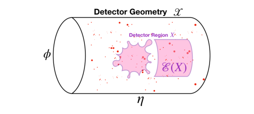
Figure 1: An illustration of the energy flow $\mathcal{E}(X)$, which is the total amount of radiation captured inside a subset $X$ (in purple) of the total detector geometry $\mathcal{X}$. The red dots represent particles that hit the detector wall, with their size proportional to their energy.

Under Def. 1, energy flows inherit a very rich and natural mathematical structure. The most important operation for our purposes is the integral of a function $\phi:\mathcal{X}\to\mathbb{R}$ against an energy flow $\mathcal{E}$, which we denote $\expectationvalue{\mathcal{E},\phi}$, defined as:

$$\expectationvalue{\mathcal{E},\phi} \equiv\int_{\mathcal{X}}dx\,\mathcal{E}(x)\,\phi(x)$$ (9)

$$=\sum_{i}E_{i}\,\phi(x_{i})\text{ for atomic flows.}$$ (10)

This operation can be thought of as the energy-weighted expectation value of the random variable $\phi$ under the distribution $\mathcal{E}$. A brief review of this, and other salient measure-theoretic concepts and definitions we call upon in this paper, is presented in App. A.

2.3 Geometrizing IRC Safety

Infrared and colinear (IRC) safety is an incredibly powerful constraint on the form of observables – it ensures not only that an observable is well-defined in perturbation theory, but also that the observable is robust to detector effects. Using the language developed in Sec. 2.2, IRC safety becomes a topological statement on the space of energy flows, which we may use to place constraints on the potential form of the universal loss function $\mathcal{L}$ of Eq. (5).

An observable $\mathcal{O}$ is IRC safe if it satisfies:

• Infrared safety: For any event atomic $\mathcal{E}$, adding or removing an $\epsilon$-soft emission to $\mathcal{E}$ leaves $\mathcal{O}$ unchanged as $\epsilon\to 0$.

• Collinear safety: For any atomic event $\mathcal{E}$, splitting any particle into two particles at the same location with the same total energy leaves $\mathcal{O}$ unchanged. Moreover, translating either particle by an $\epsilon$-small displacement leaves $\mathcal{O}$ unchanged as $\epsilon\to 0$.

Essentially, IRC safety means that observables should not change significantly if we change $\mathcal{E}$ by slightly adjusting particle energies and positions. As with energy flows, we propose a generalization of IRC safety that captures all its salient features:

Definition 2.

An observable $\mathcal{O}$ is IRC safe if it is continuous with respect to the weak* topology on energy flows.

A function $f$ on energy flows is continuous to the weak* topology if, for any sequence of energy flows $\mathcal{E}_{n}$ that converges to $\mathcal{E}$, the function $F(\mathcal{E}_{n})$ converges to $F(\mathcal{E})$ (see App. A for more details). Note that this is actually a slightly weaker constraint than the one considered in Ref. 2020 , which defines IRC safety through the metric topology induced by the EMD – the definition here does not require a metric on the space of events, or even a metric on the detector space, only a notion of continuity. In fact, there is a large class of metrics one can place on the space of events to metrize the weak* topology, not just the EMD.

An interesting consequence of this definition is that if an observable $\mathcal{O}$ is IRC safe, then $\mathcal{O}(\mathcal{E})$ for any energy flow $\mathcal{E}$ can be arbitrarily well-approximated by atomic energy flows. This implies, for example, that a continuous circle can be arbitrarily well approximated by a finite number of points arranged in a ring – this is makes possible to not only encode continuous distributions numerically, but also to make broad statements about the behavior of IRC safe observables by considering their action only on simple atomic energy flows.

In order to be IRC safe, our universal loss function $\mathcal{L}(\mathcal{E},\mathcal{E}^{\prime})$ must be continuous in both of its arguments. This is very restrictive, and immediately implies that $\mathcal{L}$ cannot have any terms that are discontinuous in either energy or distance, e.g. terms like $E^{-1}$ or $d(x,y)^{-1}$, or any term of the form $\expectationvalue{\mathcal{E},\phi}$ for noncontinuous $\phi$. Recalling the discussion in Sec. 2.1 that $\mathcal{L}$ quantifies how close in the space of energy flows $\mathcal{E}$ and $\mathcal{E}^{\prime}$ are, it is convenient (though not strictly necessary) to use $\mathcal{L}$ to metrize the weak* topology – that is, if an observable $\mathcal{O}$ is continuous with respect to the metric topology induced by $\mathcal{L}$, then it is also continuous with respect to the weak* topology, and therefore is IRC safe. This allows the same universal loss function $\mathcal{L}$ to be used both to define shape observables and to define IRC safety. This is convenient, since it captures the very intuitive notion that if two events geometrically look similar (that is, $\mathcal{L}$ is small), then IRC-safe observables evaluated on them should also be the same.

2.4 The Importance of Being Faithful

In order to encode geometric information about energy distributions, the universal loss function $\mathcal{L}$ of Eq. (5) must explicitly depend on the detector ground metric, $d(x,y)$. While there are many metrics on the space of measures that encode geometric information while also being IRC-safe (as defined in Sec. 2.3), a natural choice is the family of Wasserstein metrics, which we denote $\mathcal{L}(\mathcal{E},\mathcal{E}^{\prime})=\text{EMD}^{(\beta,R)}(\mathcal{E},\mathcal{E}^{\prime})$ (for Earth-Mover’s or Energy-Movers Distance, which we will use synonymously). We show in this section that unlike other potential candidates for $\mathcal{L}$, the Wasserstein metric will never warp distances between shapes – that is, the Wasserstein metric lifts the ground metric of the detector faithfully. A constructive proof of this can be found in App. B.

The EMD between two measures $\mathcal{E}$ and $\mathcal{E}^{\prime}$ is given by:

$$\text{EMD}^{(\beta,R)}(\mathcal{E},\mathcal{E}^{\prime})=\min_{\pi\in\mathcal{M}(\mathcal{X}\times\mathcal{X})}\left[\frac{1}{\beta R^{\beta}}\expectationvalue{\pi,d(x,y)^{\beta}}\right]+|\Delta E_{\rm tot}|,$$

$$\pi(\mathcal{X},Y)\leq\mathcal{E}^{\prime}(Y),\quad\pi(X,\mathcal{X})\leq\mathcal{E}(X),\quad\pi(\mathcal{X},\mathcal{X})=\min(E_{\rm tot},E^{\prime}_{\rm tot}),$$ (11)

where $d(x,y)$ is the ground metric between points $x$ and $y$ on $\mathcal{X}$, and $\mathcal{M}(\mathcal{X}\times\mathcal{X})$ is the space of all positive measures on $\mathcal{X}\times\mathcal{X}$. The parameter $R>0$ sets a distance scale for the EMD, and sets the relative scale for the two terms in Eq. (2.4). The parameter $\beta\geq 1$ sets the distance norm. Note that our definition of the EMD differs from Refs. Komiske_2019 ; 2020 by a factor of $\beta$, which we do to match the conventions of the geomloss feydy2019interpolating package. The additional energy difference term, $|\Delta E_{\rm tot}|$, contributes whenever the two energy flows do not have the same total energy.

The Wasserstein metric is special in that it faithfully lifts the ground metric, $d$. To lift the ground metric means that the Wasserstein metric reduces to $d(x,y)^{\beta}$ when evaluated on two point measures $\mathcal{E}\sim\delta_{x}$ and $\mathcal{E}^{\prime}\sim\delta_{y}$ – that is, the Wasserstein metric preserves distances between points. Moreover, to do so faithfully means that the Wasserstein metric preserves distances for entire extended shapes: if $\mathcal{E}$ is any measure, and $\mathcal{E}^{\prime}$ is the same as $\mathcal{E}$ whose density is translated by a vector $t$ (that is, $\mathcal{E}^{\prime}$ has corresponding density $\mathcal{E}(x-t)$), then the metric between them is simply $d(0,t)^{\beta}$.

To see this explicitly, we can compare to two other potential candidates for our universal loss function $\mathcal{L}$: the class of Maximum Mean Discrepancies (MMDs) ramdas2017wasserstein and Chamfer distances 10.5555/1622943.1622971 , which can respectively be written as:

$$\text{MMD}^{(\beta)}(\mathcal{E},\mathcal{E}^{\prime}) =-\frac{1}{2\beta}\int_{\mathcal{X}\times\mathcal{X}}dx\,dy\,d(x,y)^{\beta}\,\left(\mathcal{E}(x)-\mathcal{E}^{\prime}(x)\right)\left(\mathcal{E}(y)-\mathcal{E}^{\prime}(y)\right),$$ (12)

$$\text{CD}^{(\beta)}(\mathcal{E},\mathcal{E}^{\prime}) =\frac{1}{2\beta}\int_{\mathcal{X}}dx\,\min_{y\in{\rm Supp}(\mathcal{E}^{\prime})}[d(x,y)^{\beta}]\,\mathcal{E}(x)+\frac{1}{2\beta}\int_{\mathcal{X}}dy\,\min_{x\in{\rm Supp}(\mathcal{E})}[d(x,y)^{\beta}]\,\mathcal{E}^{\prime}(y).$$ (13)

These candidate loss functions are IRC safe, translationally invariant, and even lift the ground metric, but importantly, they do not do so faithfully. To see this, we choose the following example energy flows:

$$\mathcal{E}(x) \sim\frac{1}{2}\delta_{0}+\frac{1}{2}\delta_{a},\quad\mathcal{E}^{\prime}(x)\sim\frac{1}{2}\delta_{t}+\frac{1}{2}\delta_{a+t},$$ (14)

where $a$ and $t$ are arbitrary vectors (where $\mathcal{E}$ consists of 2 points separated by a vector $a$, and $\mathcal{E}^{\prime}$ is $\mathcal{E}$ translated by a vector $t$). A direct computation using Eqs. (2.4), (12), and (13) (with $d(x,y)=|x-y|$) yields:

$$\text{EMD}^{(\beta,R=1)}(\mathcal{E},\mathcal{E}^{\prime}) =\frac{1}{\beta}|t|^{\beta},$$ (15)

$$\text{MMD}^{(\beta)}(\mathcal{E},\mathcal{E}^{\prime}) =\frac{1}{2\beta}\left(|t|^{\beta}+\frac{1}{2}|t-a|^{\beta}+\frac{1}{2}|t+a|^{\beta}-|a|^{\beta}\right),$$ (16)

$$\text{CD}^{(\beta)}(\mathcal{E},\mathcal{E}^{\prime}) =\frac{1}{2\beta}\left(\min\left[|t|^{\beta},|t+a|^{\beta}\right]+\min\left[|t|^{\beta},|t-a|^{\beta}\right]\right).$$ (17)

While Eqs. (16) and (17) do indeed reduce to $\sim|t|^{\beta}$ when $a\to 0$ (that is, when $\mathcal{E}$ reduces to a single point), in general the MMD and Chamfer distance effectively “distort” the shape. When $\beta=1$, for instance, $\mathcal{E}^{\prime}$ appears slightly closer to $\mathcal{E}$, as measured using either MMD or the Chamfer distance, than its total displacement $|t|$ – energy in the interior of an extended distribution gets effectively “screened” by the energy in the rest of the distribution! Not only does this distortion ruin our ability to think of our observables as measuring the geometric distribution of energy in the detector, the screening effect also induces a practical issue, as it causes vanishing gradients when trying to optimize over $\mathcal{L}$ feydy2019interpolating (in this case, by minimizing $t$, for example). The Wasserstein metric does not suffer these problems, making it the natural choice for our universal loss function.

3 Hearing Shapes

Having constructed the Wasserstein metric and EMD in Sec. 2 for event and jet shapes, we next generalize Eqs. (1) and (2), which were originally introduced in Ref. 2020 as a common form for many well-known observables. We treat Eqs. (1) and (2) as definitions for shape observables $\mathcal{O}_{\mathcal{M}}$ and shape parameters $\theta_{\mathcal{M}}$, which together are the natural generalization of event and jet shapes. Moreover, we show how the manifold of energy flows $\mathcal{M}$ can be chosen to construct new observables that probe specific geometric structures. We provide a prescription for building $\mathcal{M}$, which defines the shape observable, as well as prescriptions for composing shape observables together, allowing new shape observables to be defined from simpler ones in a geometrically intuitive way.

This section proceeds as follows. First, we define generalized shape observables and shape parameters, and discuss their properties. Next, we discuss our prescription for shape composition, which can be used to define shape observables and parameters that probe complex geometric structure. Finally, we use our prescription to construct a large (but importantly, inexhaustive) suite of novel shape observables for jet substructure analysis to serve as an example of what can be done with this framework. Several examples of emperical studies using these new shape observables, evalulated using the Shaper framework defined in Sec. 4, can be found in Sec. 5.

3.1 Shape Observables and Shape Parameters

We define a shape observable $\mathcal{O}_{\mathcal{M}}$ as follows:

Definition 3.

A shape observable $\mathcal{O}_{\mathcal{M}}$, with associated shape parameters $\theta_{\mathcal{M}}$, on an energy flow $\mathcal{E}$ is any function of the form:

$$\mathcal{O}(\mathcal{E}) \equiv\min_{\mathcal{E}_{\theta}\in\mathcal{M}}{\rm EMD}^{(\beta,R)}(\mathcal{E},\mathcal{E}_{\theta}),$$ (18)

$$\theta(\mathcal{E}) \equiv\operatorname*{argmin}_{\mathcal{E}_{\theta}\in\mathcal{M}}{\rm EMD}^{(\beta,R)}(\mathcal{E},\mathcal{E}_{\theta}),$$ (19)

where $\mathcal{M}$ is a manifold of positive measures on the detector space $\mathcal{X}$, and ${\rm EMD}^{(\beta,R)}$ is the $\beta$-Wasserstein distance with length scale $R$.

Importantly, we return both the minimum EMD value, $\mathcal{O}(\mathcal{E})$, and the parameters of the shape that produced the minimum EMD, $\theta(\mathcal{E})$. For a manifold $\mathcal{M}$ of generic parameterized shapes, we refer the former as the “shapiness” of $\mathcal{E}$, and the latter as the associated “shape parameters” of $\mathcal{E}$. For example, if $\mathcal{M}$ is the manifold of $N$-(sub)jet events, then $\mathcal{O}(\mathcal{E})$ is the $N$-(sub)jettiness of $\mathcal{E}$, and $\theta(\mathcal{E})$ are the (sub)jet parameters of $\mathcal{E}$, highlighting that Eq. (18) is really a generalization of the $N$-jettiness. Intuitively, $\mathcal{O}(\mathcal{E})$ answers the question, “How much like a shape does my event look like?”, while $\theta(\mathcal{E})$ answers the question, “Which shape does my event look most like?”.

For a fixed choice of $\beta$ and scale $R$ defining the EMD, shape observables are completely specified by the choice of the manifold of energy flows $\mathcal{M}$. This choice specifies the class of shapes being considered. Practically speaking, this manifold can be defined by choosing a set of coordinates $\theta$ on the manifold, that parameterize a set of constrained energy flows $\mathcal{E}_{\theta}$. Since, as established in Sec. 2.2, energy flows are positive measures on the detector space, $\mathcal{M}$ can be built as a (weighted) parameterized probability distribution $p_{\theta}$, which is realized by a finite sampling procedure for weighted points on $\mathcal{X}$.

In Ref. 2020 , the manifold corresponding to several event and jet shapes were listed. However, the power of our framework is that any manifold of parameterized energy flows defines a valid shape observable, and moreover, this observable directly probes intuitive geometric information. By defining, for example, $\mathcal{M}$ to be the manifold of energy flows resembling uniform rings of energy, uniform disks of energy, or even uniform ellipses of energy, the corresponding observables directly quantify the diskiness, circliness, and ellipsiness of events. To our knowledge, the event isotropy Cesarotti:2020hwb is the first observable of this form with no known alternative formulation, as it quantifies the “uniforminess” of events. Examples of analyses using these custom observables can be found in Sec. 5.

Below, we list some useful properties of all shape observables:

1. Monotonicity: If $\mathcal{O}_{1}$ and $\mathcal{O}_{2}$ are defined by manifolds $\mathcal{M}_{1}$ and $\mathcal{M}_{2}$, for a fixed choice of $\beta$ and $R$, then $\mathcal{M}_{1}\supseteq\mathcal{M}_{2}$ implies that for all energy flows $\mathcal{E}$, we have $\mathcal{O}_{1}(\mathcal{E})\leq\mathcal{O}_{2}(\mathcal{E})$. This captures the monotonic nature of observables such as $N$-jettiness, which satisfy $\tau_{N+1}\leq\tau_{N}$.

2. Closure: $\mathcal{O}(\mathcal{E})=0$ if and only if $\mathcal{E}\in\mathcal{M}$. It then follows that the shape parameters $\theta(\mathcal{E})$ are such that $\mathcal{E}_{\theta}=\mathcal{E}$. In particular, this implies that for $\mathcal{M}_{\mathcal{E}}$, the space of all energy flows, $\mathcal{O}(\mathcal{E})=0$ for all events.

3. Approximation Bounds: For any $L$-Lipschitz function $\phi$ on $\mathcal{X}$, the “optimal shape” $\mathcal{E}_{\theta}$ corresponding to $\mathcal{E}$ satisfies $\frac{1}{RL}|\expectationvalue{\mathcal{E},\phi}-\expectationvalue{\mathcal{E}_{\theta},\phi}|\leq\mathcal{O}(\mathcal{E})$ Komiske_2019 . That is, the optimal shape $\mathcal{E}_{\theta}$ can be used to approximate additive Lipschitz observables on $\mathcal{E}$, up to a known bounded error.

4. Upper Bounds: If $\mathcal{X}$ is bounded by a maximum distance scale $R_{\rm max}$, and both $\mathcal{E}$ and all energy flows on $\mathcal{M}$ satisfy $E_{\rm tot}=1$, then $\mathcal{O}(\mathcal{E})$ is bounded above by $\left(\frac{R_{\rm max}}{R}\right)^{\beta}$. This can be seen by considering the extreme case where $\mathcal{E}$ and $\mathcal{E}_{\theta}$ are singleton points located $R_{\rm max}$ away from each other. Any configuration other than this will yield a lower EMD. This makes it always possible to normalize $\mathcal{O}(\mathcal{E})\in[0,1]$.

We call a manifold of energy flows $\mathcal{M}$ balanced if all of the energy flows are all normalized (i.e. $E_{\rm tot}=1)$, and unbalanced otherwise. Similarly, we call shape observable $\mathcal{O}_{\mathcal{M}}$ balanced if $\mathcal{M}$ is balanced and it is only evaluated on normalized energy flows. For a balanced observable, the choice of scale $R$ constitutes only a change of units for the distance metric, and is unimportant. Moreover, in the limit $R\xrightarrow{}\infty$, the quantity $R^{\beta}\mathcal{O}(\mathcal{E})$ is only finite if $E_{\rm tot}=E_{\theta\rm tot}$ 2020 . In this limit, the $\operatorname*{(arg)min}$ can be written over the submanifold $\mathcal{M}_{E}\subseteq\mathcal{M}$, which is the submanifold events with the same total energy as $\mathcal{E}$. Thus, the $R\to\infty$ limit effectively forces unbalanced shape observables to be balanced. We will primarily consider balanced shape observables for the remainder of this paper, though there are many important unbalanced observables (e.g. $N$-jettiness) that one may consider.

3.2 Composing Shapes

Given two shape observables $\mathcal{O}_{1}$ and $\mathcal{O}_{2}$, with the same choice of $\beta$ and $R$, we can define a new composite observable $\mathcal{O}=\mathcal{O}_{1}\oplus\mathcal{O}_{2}$. As with all shape observables above, we define the composite shape observable $\mathcal{O}$ by specifying the corresponding manifold $\mathcal{M}$. We consider two possible scenarios to define $\mathcal{M}$:

• Case 1 (Balanced): If both $\mathcal{O}_{1}$ and $\mathcal{O}_{2}$ are balanced shape observables, then we define $\mathcal{M}$ to be the manifold of all energy flows $\mathcal{E}$ of the form $\mathcal{E}=z_{1}\mathcal{E}_{1}+z_{2}\mathcal{E}_{2}$, where $\mathcal{E}_{1}\in\mathcal{M}_{1}$ and $\mathcal{E}_{2}\in\mathcal{M}_{2}$, and $(z_{1},z_{2})$ is a point in $\Delta_{1}$, the 1-simplex.

• Case 2 (Totally Unbalanced): If the energy flows on $\mathcal{M}_{1}$ and $\mathcal{M}_{2}$ have unconstrained $E_{\rm tot}$’s (that is, $E_{\rm tot}$ is an independent free parameter for each manifold), then we define $\mathcal{M}$ to be the manifold of all energy flows $\mathcal{E}$ of the form $\mathcal{E}=\mathcal{E}_{1}+\mathcal{E}_{2}$, where $\mathcal{E}_{1}\in\mathcal{M}_{1}$ and $\mathcal{E}_{2}\in\mathcal{M}_{2}$.

There exist other possible cases, such as if the manifolds only admit a small range of $E_{\rm tot}$ values, but we will not consider them in this work. In Case 1, the 1-simplex $\Delta_{1}$ introduces 2 additional (constrained) parameters to the shape, $z_{1}$ and $z_{2}$, that ensure that all energy flows are still normalized to 1, so that $\mathcal{O}$ is balanced. Here, $\mathcal{M}$ can be realized by generating points according to the parameterized sampling procedures for $\mathcal{M}_{1}$ and $\mathcal{M}_{2}$, and multiplying the energy weights of the generated particles by $z_{1}$ and $z_{2}$, respectively. The values of $z_{1}$ and $z_{2}$ control the relative contribution of each base shape to the composition. In Case 2, the total energy remains unconstrained, and the relative importance of each base shape to the contribution is controlled by the ratio of the $E_{1\rm tot}$ and $E_{2\rm tot}$ parameters. Note that monotonicity implies that, for both Case 1 and Case 2, $\mathcal{O}(\mathcal{E})\leq\mathcal{O}_{1}(\mathcal{E})$ and $\mathcal{O}(\mathcal{E})\leq\mathcal{O}_{2}(\mathcal{E})$.

It is easy to extend these definitions to a composition of $N$ observables, $\mathcal{O}=\bigoplus_{i=1}^{N}\mathcal{O}_{i}$. For the balanced case, $\mathcal{M}$ comprises of energy flows of the form $\mathcal{E}=\sum_{i=1}^{N}x_{i}\mathcal{E}_{i}$ for $\mathcal{E}_{i}\in\mathcal{M}_{i}$ and $z_{i}\in\Delta_{N-1}$. In the totally unbalanced case, $\mathcal{M}$ comprises energy flows of the form $\mathcal{E}=\sum_{i=1}^{N}\mathcal{E}_{i}$ for $\mathcal{E}_{i}\in\mathcal{M}_{i}$. When the $\mathcal{O}_{i}$ are all copies of the same shape observable $\mathcal{O}$, we define the notation $N\times\mathcal{O}$, and name the resulting composite shape observable the “$N$-shapiness”.

Given this language, we can understand several existing shape observables as composites of basic “shape” building blocks. For instance, we can define an observable, the (sub)pointiness $\tau_{1}(\mathcal{E})$, corresponding to the manifold of weighted (normalized) $\delta$-function measures on $\mathcal{X}$. Geometrically, this observable to fitting a single weighted (normalized) point to an event $\mathcal{E}$, the former with a floating energy weight. We can then define the $N$-(sub)pointiness of $\mathcal{E}$ to be $\tau_{N}(\mathcal{E})=N\times\tau_{1}(\mathcal{E})$ – this is exactly the $N$-(sub)jettiness of $\mathcal{E}$, with $N$-subjettiness corresponding to balanced composition, and $N$-jettiness corresponding to totally unbalanced composition.

Shape composition provide a novel avenue for understanding event and jet substructure. For example, the observable $\tau_{N}\oplus\mathcal{I}$, where $\mathcal{I}$ is the event isotropy, can be thought of as a “pileup-corrected” $N$-(sub)jettiness, where a uniform background is subtracted off. One can use this observable to probe the percentage of energy deposited in hard jets versus a uniform background due to pileup Soyez:2018opl and underlying event effects PhysRevD.65.092002 ; Agocs:2010ft . In particular, the shape parameter $\theta(\mathcal{E})=z_{1}(\mathcal{E})$ is an estimate of the percentage of energy in $E$ due to hard jets. In Sec. 5.7, we consider perform empirical studies of these types of shape observables.

3.3 Examples of Novel Shapes

In this subsection, we list (some) potentially phenomenologically interesting shape observables, all of which are defined for the first time in this work, that can be constructed using the prescription outlined above. For all these observables, we consider the detector geometry to be a rectangular patch of a cylinder, $\mathcal{X}=[y_{\rm min},y_{\rm max}]\times[\phi_{\rm min},\phi_{\rm max}]$, though one could consider the full cylinder as well. These observables are summarized in Table 3, and we show empirical examples of these observables in action in Sec. 5. We consider balanced observables with $\beta=1$, leaving unbalanced observables for future work.

Sec.	Shape	Specification	Illustration
3.3.1	Ringiness	Manifold of Rings
	$\mathcal{O}_{R}$	$\mathcal{E}_{x_{0},R_{0}}(x)=\frac{1}{2\pi R_{0}}$ for $|x-x_{0}|=R_{0}$
		$x_{0}$ = Center, $R_{0}$ = Radius
3.3.2	Diskiness	Manifold of Disks
	$\mathcal{O}_{D}$	$\mathcal{E}_{x_{0},R_{0}}(x)=\frac{1}{\pi R_{0}^{2}}$ for $|x-x_{0}|\leq R_{0}$
		$x_{0}$ = Center, $R_{0}$ = Radius
3.3.3	Ellipsiness	Manifold of Ellipses
	$\mathcal{O}_{E}$	$\mathcal{E}_{x_{0},a,b,\varphi}(x)=\frac{1}{\pi ab}$ for $x\in\text{Ellipse}_{x_{0},a,b,\varphi}$
		$x_{0}$ = Center, $a,b$ = Semi-axes, $\varphi$ = Tilt
3.3.4	(Ellipse	Composite Shape
	$+$Point)iness	$\mathcal{O}_{E}\oplus\tau_{1}$
		Fixed to same center $x_{0}$
3.3.5	N-(Ellipse	Composite Shape
	$+$Point)iness	$N\times(\mathcal{O}_{E}\oplus\tau_{1})\oplus\mathcal{I}$
	$+$Pileup

Table 3: Custom observables, defined using the Shaper prescription, designed to probe jet substructure at increasing levels of complexity. For each observable, the manifold parameterization is given, either explicitly, or as a composition of previously defined objects. Here, $\tau_{1}$ is the one-pointiness (1-subjettiness), and $\mathcal{I}$ is the event isotropy. More details on these types of observables, plus explicit construction of sampling functions, can be found in Sec. 3.3.

3.3.1 $N$-Ringiness

We first consider a simple shape observable: ringiness, which probes how ring-like an event is. We begin by defining the manifold of all ring-like energy flows $\mathcal{M}_{R}$, which consist of energy flows corresponding to energy flow densities of the form:

$$\mathcal{E}_{x_{0},R_{0}}(x)=\begin{cases}\frac{1}{2\pi R_{0}}&|x-x_{0}|=R\\ 0&\text{otherwise}\end{cases},$$ (20)

where the parameters $x_{0}$ and $R_{0}$ correspond to the center and radius of a ring, respectively. To build a sampler, we use the so-called reparameterization trick https://doi.org/10.48550/arxiv.1506.02557 . Drawing $N$ samples from the unit uniform distribution $\phi\sim U(0,1)$, the distribution of points:

$$x=R_{0}\left(\cos(2\pi\phi),\sin(2\pi\phi)\right)+x_{0},$$ (21)

where each particle has weight $\frac{1}{N}$, is a realization of $\mathcal{E}_{x_{0},R_{0}}(x)$.

The corresponding observable, $\mathcal{O}_{R}(\mathcal{E})$, is the ringiness of the event $\mathcal{E}$. While most QCD jets are not expected to be ring-like, this observable can identify clumps of radiation scattered around a central point, as may be the case in a 3-pronged top quark decay. Additionally, observables that probe the boundary of a jet with an empty interior may prove useful in studies of the dead-cone effect Dokshitzer:1991fc ; Dokshitzer:1991fd ; PhysRevLett.69.3025 where collinear radiation is relatively suppressed.

Having defined ringiness, we can next define $N$-ringiness, which probes how much an event looks like $N$ rings, each of arbitrary center, radius, and weight. This observable is defined as $N\times\mathcal{O}_{R}$. Following the prescription outlined in Sec. 3.2, we can build $N$ weighted rings, by separately sampling Eq. (21) for each ring’s center and radius, and multiplying the weights by $z_{i}\in\Delta_{N-1}$.

For numerical methods, one must set initial values for these parameters in an IRC-safe way. While in principle, the choice of initialization should make no difference, in practice, the presence of numerical effects and local minima make the choice of initialization important. In our initialization scheme for $N$-rings, we perform $k_{T}$ clustering to find $N$ subjets. The location of the subjets is then taken to be the ring center, and the subjet energy is taken to be the ring energy. We choose to initialize the radius of each ring to zero, so that the $N$-ringiness is guaranteed to only deviate from $N$-subjettiness only if it will make the event more ringlike, though it is also possible to initialize the radius to e.g. the distance of the $(N+1)$-th jet in the clustering history.

3.3.2 $N$-Diskiness

Next, we define diskiness $O_{D}$, which measures how much like a disk an event is. Similar to ringiness, we parameterize the manifold of energy flow densities:

$$\mathcal{E}_{x_{0},R_{0}}(x)=\begin{cases}\frac{1}{\pi R_{0}^{2}}&|x-x_{0}|\leq R\\ 0&\text{otherwise}\end{cases},$$ (22)

where $x_{0}$ and $R_{0}$ are the center and radius of the disk.

To build a sampler, as with ringiness, we draw $N$ samples from the unit uniform distribution $\phi\sim U(0,1)$, and also $N$ points $r\sim U(0,1)$. Then, the distribution of points:

$$x=\sqrt{r}R_{0}\left(\cos(2\pi\phi),\sin(2\pi\phi)\right)+x_{0},$$ (23)

where each particle has weight $\frac{1}{N}$, is a realization of a uniform disk. The random variable $r$ controls the radius of the point being sampled, and the square root is from a Jacobian factor to make the disk uniform.

Given the diskiness, we can easily compose the $N$-diskiness, $N\times\mathcal{O}_{D}$. The $N$-diskiness is analogous to the $N$-jettiness/XCone jet algorithm, in that it returns the locations of conical clusters of particles. However, unlike XCone, the radius $R_{0}$ is a learned, rather than fixed parameter, allowing for dynamic jet radii. To initialize the $N$-diskiness, the exact same procedure is used as described in Sec. 3.3.1 for $N$-ringiness. Note that there are many ways to modify the $N$-diskiness to produce similar observables – for example, one can replace the uniform disks with Gaussians to probe different radiation patterns.

3.3.3 $N$-Ellipsiness

Jets need not necessarily be circular! Indeed, many jet algorithms, such as the widely-used $k_{T}$ Cacciari:2008gp and Cambridge-Aachen Dokshitzer:1997in ; Wobisch:1998wt algorithms, do not return circular jets. Motivated by this, we define a generalization of diskiness, the ellipsiness $\mathcal{O}_{E}$ of a jet. The manifold of ellipses is given by energy flow densities of the form:

$$\mathcal{E}_{x_{0},a,b,\varphi}(\vec{x})=\begin{cases}\frac{1}{\pi ab}&\left(\frac{(x-x_{0})\cos\varphi+(y-y_{0})\sin\varphi}{a}\right)^{2}+\left(\frac{(y-y_{0})\cos\varphi-(x-x_{0})\sin\varphi}{b}\right)^{2}\leq 1\\ 0&\text{otherwise}\end{cases},$$ (24)

$x_{0}$ is the center of the ellipse, $a$ and $b$ are the semi-major and semi-minor axes, and $\varphi$ is the tilt of the $x$-axis. Here, we have restored vector notation $\vec{x}$ to indicate that the $x$-and $y$-axes are treated differently. There are many equivalent alternate parameterizations of the ellipse, including in terms of its focal length $c=\sqrt{\max(a,b)^{2}-\min(a,b)^{2}}$ and eccentricity $e=\sqrt{1-\frac{\min(a,b)}{\max(a,b)}}$. Note that for $a=b$, the ellipse reduces to a disk, and the $\varphi$ parameter becomes redundant.

The sampling procedure for disks can be recycled for ellipses, with some small modifications. Given $N$ sampled points $\phi,r\sim U(0,1)$, the distribution:

$$x=U_{\varphi}\cdot\left(a\sqrt{r}\cos(2\pi\phi),b\sqrt{r}\sin(2\pi\phi)\right)^{T}+x_{0},$$ (25)

where $U_{\varphi}$ is the $2\times 2$ rotation matrix corresponding to the angle $\varphi$ and each particle has weight $\frac{1}{N}$, is a realization of a uniform ellipse. We can then easily compose the $N$-ellipsiness, which can serve as a jet algorithm that finds non-circular jets. In particular, this shape observable allows for the eccentriciy $e$ of the clustered jets to be extracted, allowing one to quantify how far from circular each jet is. As with the $N$-ringiness and $N$-diskiness, the centers of the ellipses are chosen using the $k_{T}$ clustering algorithm. Both $a$ and $b$ are initialized to be zero, so that deviations from either $N$-subjettiness or $N$-diskiness occur if it makes the event more elliptical.

3.3.4 … Plus Pointiness

Energy is not uniformly distributed within a jet! Indeed, to leading order in perturbative QCD, much of a jet’s radiation will be soft and/or collinear with respect to the emitting parton. We can probe this by composing together shapes that explicitly target soft and collinear radiation separately. To this end, we construct a set of new observables, the (shape$+$point)iness, for $\textit{shape}\in\{\mathcal{O}_{R},\mathcal{O}_{D},\mathcal{O}_{E}\}$. This is defined using the shape composition prescription described in Sec. 3.2, as:

$$\mathcal{O}_{i}^{\tau}=\mathcal{O}_{i}\oplus\tau_{1},$$ (26)

where $\tau_{1}$ is the 1-pointiness (equivalently, the 1-subjettiness), and $\mathcal{O}_{i}$ is any of $\{\mathcal{O}_{R},\mathcal{O}_{D},\mathcal{O}_{E}\}$ previously defined. Importantly, we fix the location of the $\delta$-function in $\tau_{1}$ to be $x_{0}$, though one may consider letting the location of the $\delta$-function float to define a recoil-free variant. We can then extend this definition to compose the $N$-(shape$+$point)iness.

When used as a jet algorithm, the $N$-(shape$+$point)iness provides a more physical picture of perturbative QCD than do the previously defined shapes. The base shapes, particularly disks and ellipses, capture wide-angle soft radiation, while the $\delta$-functions capture both hard and soft collinear radiation at the center of the (sub)jet. Moreover, within each shape-point pair, the floating parameters $z_{1}$ and $z_{2}$ tell us the fraction of radiation in the wide-angle and collinear sectors, which in principle can be calculated in and compared to perturbative QCD.

When initializing observables of this type, the initialization occurs as described in previous sections using the $k_{T}$ algorithm with all radii set to zero. However, we choose to split the $k_{T}$ energy equally between the shape and the $\delta$-function. Note that this is an IRC-safe choice, since at zero radius, the shape is indistinguishable from the $\delta$-function.

3.3.5 … Plus Pileup

In hadron-hadron collisions, there are many sources of contamination in jets, including underlying event contributions from proton remnants PhysRevD.65.092002 ; Agocs:2010ft , and pileup due to simultaneous hadron collisions Soyez:2018opl . We will collectively refer to these sources of contamination as pileup for simplicity. Pileup contamination biases and smears the “true” value of observables reconstructed from final state particles, driving the need for mitigation techniques.

Pileup is approximately uniformly distributed in the rapidity-azimuth plane. This is exactly the shape probed by the event isotropy, $\mathcal{I}$. Thus, in order to protect shape observables against pileup contamination, we can compose them with the event isotropy, which will soak up radiation uniform in the plane. This defines the shapines$+$pileup observable:

$$\mathcal{O}^{\mathcal{I}}_{i}=\mathcal{O}_{i}\oplus\mathcal{I},$$ (27)

where $\mathcal{O}_{i}$ is any shape observable, including those previously defined. As a departure from Ref. Cesarotti:2020hwb , we realize the uniform event by randomly sampling in the plane, rather than defining a grid. We also primarily focus on the $\beta=1$ event isotropy. Unlike mitigation techniques such as area subtraction Cacciari_2008 ; Cacciari_2008_2 ; Soyez:2012hv or jet grooming Larkoski:2014wba ; Dasgupta_2013 , where an implicit assumption is made about the pileup energy density (either explicitly as an input $\rho$, or implicitly through a soft scale $z_{\rm cut}$), the shape observable $\mathcal{O}^{\mathcal{I}}_{i}$ makes no explicit energy scale assumptions. The uniform energy weight, $z_{2}$, is optimized over, and so the observable “learns” its own pileup scale, which can then be extracted. We choose to initialize the pileup scale $z_{2}$ to zero, though one could choose any value of $z_{2}$ if they had a prior on the amount of pileup in events.

3.3.6 … And More!

This has not been an exhaustive list – one can use any manifold $\mathcal{M}$ of energy flows one can think of, with the only two limits being imagination and the ability to write down a sampling procedure. Other examples of shapes include polygons, hardcoded jet topologies (for example, two-pronged jets restricted to between $\Delta R=R_{1}$ and $R_{2}$ apart), Gaussian clusters, graph-based shapes, and so on. These observables can also be combined into more complex ones using shape composition. All of these can be constructed within the Shaper framework (more details in Sec. 4), and we encourage the community to use this prescription to develop their own observables.

4 The Shaper Framework

Calculating the Wasserstein metric in Eq. (2.4) is notoriously difficult; if both events have $n$ particles, then the runtime needed by a brute force, generic Wasserstein solver can be as high as $\mathcal{O}(n^{3}\log{n})$ alt_17 . Generic solvers also make it difficult to extract the gradients of the metric with respect to one of the events, $\nabla_{\mathcal{E}}\text{EMD}(\mathcal{E},\mathcal{E}^{\prime})$, which are necessary for performing gradient descent over the space of events in $\mathcal{M}$. Fortunately, by using the (de-biased) Sinkhorn divergence, which uses an $\epsilon$-regularization to approximate the Wasserstein metric, the total costs can be lowered all the way down to $\mathcal{O}({n^{2}}\log{n})$ sink_n2ln(n) ; Sink_ICML_19 ; sink_nlogn ; sink_n_comp ; wass_n3_input_dist ; feydy2019interpolating .

In this section, we introduce the Shape Hunting Algorithm for Parameterized Energy Reconstruction – or Shaper – to define and calculate shape observables. Shaper is a Pytorch-enabled NEURIPS2019_9015 and parallelized computational framework for defining and composing shape observables and their corresponding energy flow manifolds, built using the geomloss feydy2019interpolating package. We start by outlining the Shaper algorithm. Then, we provide details on the Sinkhorn divergence, before ending this section with implementation details. For the rest of this paper, we restrict ourselves to balanced observables, i.e. $E_{\theta,{\rm tot}}=E_{\rm tot}=1$, leaving the unbalanced case for future work.

4.1 The Shaper Algorithm

We now describe how to perform the minimization $\operatorname*{(arg)min}_{\mathcal{E}^{\prime}_{\theta}\in\mathcal{M}}\left[\text{EMD}(\mathcal{E},\mathcal{E}^{\prime}_{\theta})\right]$ using Shaper. The Shaper algorithm for estimating shape observables on an event is as follows:

1. Define: Following the prescription of Sec. 3.1, define a manifold $\mathcal{M}$ and coordinates $\theta$ parametrizing the manifold. Define the ground metric $d(x,y)$, the exponent $\beta$, and the radius $R$. This fully defines the observable $\mathcal{O}$. Build a sampling function $p_{\theta}$ that uses the parameters $\theta$ to transform some base distribution into a realization of the energy flows $\mathcal{E}^{\prime}_{\theta}\in\mathcal{M}$. Finally, choose an approximation parameter $\epsilon\ll 1$ and an annealing parameter $\Delta\in(0,1)$.

2. Initialize: For each event $\mathcal{E}$, choose initial parameters $\theta$. This initialization should be done in an IRC-safe way.

3. Compute the EMD: Compute the de-biased Sinkhorn divergence, $S_{\epsilon}(\mathcal{E},\mathcal{E}^{\prime})$, as defined in Sec. 4.3 below, as an estimate of the EMD. Save the corresponding de-biased Kantorovich potentials, $F$ and $G$.

4. Gradient Update: Perform the gradient update:

   $$\theta\xleftarrow{}\theta-\alpha\left(\sum_{j=1}^{M}G(y_{j})\partialderivative{E^{\prime}_{j}}{\theta}+\sum_{j=1}^{M}E^{\prime}_{j}\partialderivative{G(y_{j})}{y_{j}}\partialderivative{y_{j}}{\theta}\right),$$ (28)

   where $\alpha$ is a learning rate hyper-parameter. The first term is the dependence of the EMD on particle energies due to $\theta$, and the second is the dependence due on particle positions due to $\theta$, both of which are implicit through the sampling function $p_{\theta}$. This step can be replaced with any other gradient descent optimizer.

5. Constrain: If the manifold $\mathcal{M}$ is nontrivial, impose any necessary constraints on the coordinates $\theta$, such as wrapping angles between $-\pi$ and $\pi$, enforcing positivity, or a simplex projection.

6. Converge: Repeat Steps 3–5 until convergence. Return the final value of the EMD and the final $\theta$ parameters.

The Shaper framework contains modules to aid or automate each of these steps, which we describe further in Sec. 4.4.

4.2 The Dual Formulation of Wasserstein

Observe that the EMD in Eq. (2.4) falls into a generic class of problems called linear programs. A linear program involves minimizing a function $\mathcal{L}(x)=\expectationvalue{c,x}$ over vectors $x$, where $c$ is some cost function linear in $x$. Furthermore, $x$ satisfies some linear constraint of the form $b=Ax$, and we additionally require $x\geq 0$. In our case, $x$ is the (flattened) transfer matrix $\pi$, $c$ is the (flattened) distance matrix $d^{\beta}$, $b=(\mathcal{E},\mathcal{E}^{\prime})$ are the energy flows, and $A$ is a matrix enforcing the simplex constraints on $\pi$.

The theory of linear programs is well-studied gartner_06 . In particular, for every primal linear program, there exists a dual linear program, where the constraints and variables to be optimized switch roles, similar to the method of Lagrange multipliers. In the dual problem, one instead maximizes the function $\mathcal{L}(y)=\expectationvalue{b,y}$, subject to $A^{T}y\leq c$. For the Wasserstein metric, the dual formulation looks like:

$$\text{EMD}(\mathcal{E},\mathcal{E}^{\prime})^{(\beta,R)} =\max_{f,g:\mathcal{X}\to\mathbb{R}}\left[\expectationvalue{\mathcal{E},f}+\expectationvalue{\mathcal{E}^{\prime},g}\right],\text{ such that }f(x)+g(y)\leq\frac{1}{\beta R^{\beta}}d(x,y)^{\beta},$$ (29)

where $f$ and $g$ are known as the dual potentials or Kantorovich potentials. This formulation of the EMD is known as the Kantorovich–Rubinstein metric Vilani_03 .

In this form, the EMD has several nice properties. First, the arguments $\mathcal{E}$ and $\mathcal{E}^{\prime}$ are explicit, rather than implicit in the form of constraints. This makes taking the gradient of the EMD with respect to either energy flow much easier. This property is incredibly useful for performing optimizations over energy flows, since it enables easy differentiation. Second, the optimization over an $MN$-dimensional object, $\pi_{ij}$, is replaced by an optimization over the $(M+N)$-dimensional object, $f_{i}$ and $g_{j}$, making the simplex constraint structure more apparent. It can be shown that the optimal choice of $f$ and $g$ actually saturates the bound in Eq. (29) feydy_20 . Recalling that the ground metric satisfies $d(x,x)=0$ for all $x$, we can see that the optimal $f,g$ pair satisfies $f(x)=-g(x)$. This allows us to rewrite the constraint as:

$$|f(x)-f(y)|\leq\frac{1}{\beta R^{\beta}}d(x,y)^{\beta}.$$ (30)

That is, $f$ is $\beta$-Hölder continuous. Note that for $\beta=1$, this reduces to Lipschitz continuity on $f$.

4.3 Reviewing the Sinkhorn Divergence

The source of the difficulty in evaluating Eq. (29) is the highly nonconvex optimization. To alleviate this, we introduce a regulator cuturi2013sinkhorn ; CLASON2021124432 to the dual Wasserstein metric:

$${\rm OT}^{(\beta,R)}_{\epsilon}(\mathcal{E},\mathcal{E}^{\prime})=\max_{f,g:\mathcal{X}\xrightarrow[]{}\mathbb{R}}\Biggl{[} \expectationvalue{\mathcal{E},f}+\expectationvalue{\mathcal{E}^{\prime},g}$$

$$-\epsilon^{\beta}\log\expectationvalue{\mathcal{E}(x)\otimes\mathcal{E}^{\prime}(y),e^{\left(\frac{1}{\epsilon^{\beta}}(f(x)+g(y)-\frac{1}{\beta R^{\beta}}d(x,y)^{\beta})\right)}}\Biggr{]},$$ (31)

where $\epsilon$ is a regulation parameter. The quantity ${\rm OT}^{(\beta,R)}_{\epsilon}(\mathcal{E},\mathcal{E}^{\prime})$ is known as the Sinkhorn divergence sinkhorn_1966 between measures $\mathcal{E}$ and $\mathcal{E}^{\prime}$. It reduces to the EMD as $\epsilon\to 0$. Notably, for any $\epsilon>0$, the optimization over $f$ and $g$ is fully convex feydy_20 , making the minimum significantly easier to evaluate.

Note that there are no constraints on the functions $f$ and $g$ anymore. Instead, the maximum will only be achieved when $f(x)+g(y)$ is within order $\epsilon^{\beta}$ of $\frac{1}{\beta R^{\beta}}d(x,y)^{\beta}$, a softer version of the original simplex constraint. We can view the parameter $\epsilon$ as “blurring” the distance metric $d(x,y)$, where $\epsilon$ is a distance scale measured in units of $R$.

As an unconstrained, convex minimization problem, we can estimate the Sinkhorn divergence using simple gradient descent by taking derivatives of Eq. (31) with respect to $f$ and $g$. Given two atomic measures, $\mathcal{E}$ and $\mathcal{E}^{\prime}$, with $M$ and $N$ particles respectively, and an approximation parameter $\epsilon$, we estimate the Kantorovich potentials $f(x_{i})$ and $g(y_{j})$ that give us the Sinkhorn divergence using the following algorithm:

1. Initialize: Initialize $f(x_{i})=0$ and $g(y_{j})$ = 0.

2. Gradient Update: Update $f$ and $g$ simultaneously as follows:

   $$f(x_{i}) \xleftarrow{}-\epsilon^{\beta}\log(\sum_{j=1}^{N}E^{\prime}_{j}e^{\left(\frac{1}{\epsilon^{\beta}}(g(y_{j})-\frac{1}{\beta R^{\beta}}d(x_{i},y_{j})^{\beta})\right)}),$$ (32)

   $$g(y_{j}) \xleftarrow{}-\epsilon^{\beta}\log(\sum_{i=1}^{M}E_{i}e^{\left(\frac{1}{\epsilon^{\beta}}(f(x_{i})-\frac{1}{\beta R^{\beta}}d(x_{i},y_{j})^{\beta})\right)}).$$ (33)

3. Converge: Repeat Step 2 until convergence. Return the Kantorovich potentials $f$ and $g$, and the Sinkhorn Divergence Eq. (31) evaluated on these potentials.

This algorithm is known to converge in finite time sinkhorn_1966 ; sinkhorn1967diagonal ; sinkhorn1967concerning . The runtime of each iteration scales as approximately $\mathcal{O}((M+N)^{2})$, and the algorithm converges in approximately $\frac{1}{\epsilon^{\beta}}$ iterations. This can be further improved to only $\log(\frac{1}{\epsilon^{\beta}})/\log(\frac{1}{\Delta})$ iterations through the use of simulated annealing KOSOWSKY1994477 ; Bertsekas , with a parameter $\Delta\in(0,1)$. Beginning with a larger effective blurring radius $\epsilon^{\prime}=2R$, after every iteration of the Sinkhorn algorithm, we decrease $\epsilon^{\prime}\xleftarrow{}\Delta\epsilon^{\prime}$, until finally reaching $\epsilon^{\prime}=\epsilon$. Intuitively, we start with a large blurring scale $R$, and slowly “zoom in” to a distance scale of $\epsilon$ to refine the estimate of the Sinkhorn divergence.

However, the Sinkhorn divergence is biased, meaning that it is not generically the case that ${\rm OT}_{\epsilon}(\mathcal{E}^{\prime},\mathcal{E}^{\prime})=0$, which is an important property of the Wasserstein metric. We use therefore the de-biased Sinkhorn divergence, defined in Ref. feydy2019interpolating :

$$S_{\epsilon}(\mathcal{E},\mathcal{E}^{\prime})={\rm OT}_{\epsilon}(\mathcal{E},\mathcal{E}^{\prime})-\frac{1}{2}{\rm OT}_{\epsilon}(\mathcal{E},\mathcal{E})-\frac{1}{2}{\rm OT}_{\epsilon}(\mathcal{E}^{\prime},\mathcal{E}^{\prime}).$$ (34)

The de-biased Sinkhorn divergence satisfies $S_{\epsilon}(\mathcal{E},\mathcal{E})=0$ by construction. This can be easily realized algorithmically by simply substituting new de-biased Kantorovich potentials $f\to F$ and $g\to G$, where

$$F(x) =f(x)-\tilde{f}(x),$$ (35)

$$G(y) =g(y)-\tilde{g}(y).$$ (36)

Here, the notation $\tilde{f}(x)$ refers to the first Kantorovich potential corresponding to $\text{OT}_{\epsilon}(\mathcal{E},\mathcal{E})$, and $\tilde{g}(y)$ refers to the second Kantorovich potential corresponding to $\text{OT}_{\epsilon}(\mathcal{E}^{\prime},\mathcal{E}^{\prime})$. For the rest of this paper, we refer to the de-biased Sinkhorn divergence as simply the Sinkhorn divergence wherever there is no chance for confusion.

In addition to returning the Sinkhorn divergence, this algorithm also returns the Kantorovich potentials, which allow us access to approximate gradients of the EMD, which can be used for shape parameter optimization. The gradients of the EMD with respect to the input measures can be read off of Eq. (31):

$$\nabla_{\mathcal{E}}\text{EMD}(\mathcal{E},\mathcal{E}^{\prime}) =F\quad\Rightarrow{}\quad\begin{cases}\quad\nabla_{E_{i}}\text{EMD}(\mathcal{E},\mathcal{E}^{\prime})=F(x_{i}),\\ \quad\nabla_{x_{i}}\text{EMD}(\mathcal{E},\mathcal{E}^{\prime})=E_{i}\nabla F(x_{i}),\end{cases}$$

$$\nabla_{\mathcal{E}^{\prime}}\text{EMD}(\mathcal{E},\mathcal{E}^{\prime}) =G\quad\Rightarrow{}\quad\begin{cases}\quad\nabla_{E_{j}^{\prime}}\text{EMD}(\mathcal{E},\mathcal{E}^{\prime})=G(y_{j}),\\ \quad\nabla_{y_{j}}\text{EMD}(\mathcal{E},\mathcal{E}^{\prime})=E_{j}^{\prime}\nabla G(y_{j}).\end{cases}$$ (37)

4.4 Implementation Details

Before turning to our case study, we discuss the specific details of the Shaper implementation. Shaper uses the geomloss package as a backend for computing Sinkhorn divergences, as described in Sec. 4.3. By default, we use a relatively conservative annealing value of $\Delta=0.9$, and choose $\epsilon^{\beta}=10^{-3}$ for our estimates. Currently, the Shaper algorithm is implemented only for balanced observables, with either $\beta=1$ or $2$.

Once the EMD and Kantorovich potentials are estimated using the geomloss backend, the gradient updates in Step 4 are then handled using automatic differentiation and backpropagation in pytorch. One may select from a suite of common machine learning optimizers to perform the gradient update – by default, we use the Adam optimizer https://doi.org/10.48550/arxiv.1412.6980 , with a learning rate of 0.01. Steps 3–5 can be easily parallelized over batches of hundreds of events at once. This is accomplished by treating the parameters $\theta$ for each $\mathcal{E}_{n}$ to be completely independent. The Sinkhorn divergence can be computed on many events at once, and since the parameters are independent, we take advantage of highly parallelized pytorch operations to perform independent derivatives $\nabla_{\theta_{n}}$ of the combined batch loss, $\sum_{n}\text{EMD}(\mathcal{E}_{n},\mathcal{E}^{\prime}_{\theta_{n}})$, all at once.

When using Shaper, one must specify a maximum number of epochs, so that the program eventually halts even if convergence is not achieved. We set this number by default to be 500 epochs, though we observe that convergence happens far earlier than this. We define convergence through an early stopping procedure: if an event’s EMD has not decreased in at least $N_{\max}$ epochs, stop early, and return the minimum EMD ever achieved during the training, and the parameters that achieved that minimum. When training on a large batch of events, we stop early when a certain fixed percentage (we choose 95% by default) have hit this condition – this is because there tends to be a handful of outlier events that take exceptionally long to converge. We choose $N_{\max}=25$ epochs by default. Both this, and the batch stopping percentage, are adjustable user parameters.

To facilitate Steps 1 and 2 of the Shaper algorithm, where the user input occurs, many common manifolds, such as sets of $N$ points, hypercubes, simplices, and so on, are already pre-built. These pre-built “building-block” manifolds are listed in Table 4. From these, more complex manifolds can be easily constructed, such as the rings, disks, and ellipses described in Sec. 3.3. The $\oplus$ and $N\times$ operators make it very easy to define new composite observables from old ones and quickly build sophisticated shapes. Parameters can also be easily frozen for more customization. Furthermore, it is straightforward to define more building-block manifold as needed within the framework. Each of the observables described in Sec. 3.3 is also pre-built into Shaper. When defining custom manifolds that use the $N$-points as a building block, the custom shape will automatically use the same IRC-safe $k_{T}$-clustering initialization scheme as the observables in Sec. 3.3, though it is possible to modify the initialization scheme as needed.

Manifold	Description	Constraints
Trivial	The set $\{0\}$	None
$N$-Points, $\mathcal{X}^{N}$	Set of $N$ points, $x_{i}$, in $\mathbb{R}^{2}$	None
Positive Reals, $\mathbb{R}^{N}_{\geq 0}$	Set of $N$ positive numbers, $R_{i}$	Clipped to $R_{i}\geq 0$
Hypercube, $\Lambda^{N}$	Set of $N$ numbers, $\lambda_{i}$, between 0 and 1	Clipped to $0\leq\lambda_{i}\leq 1$
Circle / Torus, $S^{N}$	Set of $N$ angles, $\phi_{i}$	Wrapped to $-\pi\leq\phi_{i}<\pi$
$N$-Simplex, $\Delta_{N}$	Set of $N+1$ numbers, $z_{i}\geq 0$, summed to 1	Simplex projection

Table 4: The building-block manifolds implemented in Shaper, from which parameters can be defined and more complex manifolds can be built. For each manifold, a description is given, and constraint instructions are provided to project points onto the manifold. Note that we do not distinguish here between “positive” reals versus “non-negative” reals, since for continuous parameterizations there is no difference between including zero and getting arbitrarily close to zero.

Each manifold contains instructions on how to enforce parameter constraints (as needed for Step 5). For most manifolds, this usually involves clipping the values to be within a desired range, though for the simplex $\Delta_{N}$, which occurs in almost every shape for which energy weights must be normalized, the enforcement is nontrivial. We use a simplex projection algorithm, inspired by the $K$-Deep-Simplex framework tankala2020k and its nonlinear extension mueller2022geometric , which solves the linear program https://doi.org/10.48550/arxiv.1309.1541 :

$$\min_{z_{i}}\left[\sum_{i}^{N+1}|z_{i}-y_{i}|^{2}\right]\text{ such that }\sum_{i}^{N+1}z_{i}=1,z_{i}\geq 0,$$ (38)

which finds the simplex $z_{i}\in\Delta_{N}$ closest to a set of unnormalized points $y_{i}$.

5 Empirical Studies with Jets

We now use the Shaper framework and custom shape observable in example collider physics analyses. We begin by benchmarking the Shaper algorithm, testing the performance of the Sinkhorn divergence and the optimization procedure by comparing the jet isotropy and $N$-subjettiness calculated using Shaper to other methods. Next, we calculate the ring, disk, and ellipse-based observables defined in Sec. 3.3 for a dataset of top and QCD jets, showing visualizations of each shape and analyzing the learned EMD’s and parameters. Finally, we explore the potential to use shape observables for automatic pileup removal.

5.1 Dataset

For our empirical studies, we use the top tagging benchmark of Refs. Butter:2017cot ; Kasieczka:2019dbj , which is a dataset consisting of a top quark jet signal and a mixed light-quark/gluon jet background. These samples are generated in Pythia 8.2.15 Sjostrand:2014zea at 14 TeV, and then passed through Delphes 3.3.2 deFavereau:2013fsa to simulate the ATLAS detector. Jets are defined using the anti-$k_{T}$ algorithm Cacciari:2008gp in FastJet 3.1.3 Cacciari:2011ma with $R=0.8$. Only the leading jet in any event is considered, and we select jets satisfying $p_{T,J}\in[475,525]\,\text{GeV}$ and $|\eta_{J}|<2$. The signal and background samples are generated using $t\bar{t}$ and QCD dijet events respectively. For signal top jets, a top parton, plus its decay products, are required to be within $\Delta R=0.8$ of the jet axis. All events are translated such that the jet axis is at $(0,\,0)$ on the rapidity-azimuth plane.

In this dataset, multiple parton interactions and pileup have not been included. To mock up the effects of pileup contamination in data, we add in pileup “by hand”. To each event, we add in $N$ particles randomly distributed in an $R\times R=0.8\times 0.8$ square centered at the origin on the rapidity-azimuth plane, where $N$ is Poisson-distributed with a mean of 75. Each particle is given an energy weight randomly sampled from a normal distribution with mean $\frac{E_{\rm PU}}{N}$ and standard deviation $\frac{E_{\rm fluct}}{N}$, where we take $E_{\rm PU}$, which represents the total amount of pileup radiation, to be uniformly distributed between $50$ and $250$ GeV, and $E_{\rm fluct}$, which represents per-particle fluctuations, to be $25$ GeV. Many refinements of this simplistic mockup could be considered, but this suffices to show qualitative features of Shaper and the shape observables defined in Sec. 3.3. For the purposes of calculating shape observables, all jets are normalized such that $E_{\rm tot}=1$, though we save the original total energy of each jet for the purpose of restoring units.

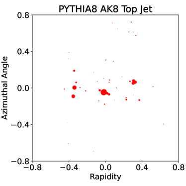
(a)

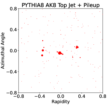
(b)

   

Figure 2: Example of a top jet (signal) event in our dataset, (a) before and (b) after the pileup mock-up procedure described in Sec. 5.1. Each red point is a single particle, and the size of the point is proportional to the relative energy of the particle.

An example top jet is shown in Fig. 2, before and after pileup is added, to illustrate this procedure. This contamination procedure is performed for the benchmarking studies in Secs. 5.2 and 5.3 and the pileup studies in Sec. 5.7. For the jet substructure studies in Secs. 5.5 and 5.6, we do not add any pileup, and instead we require that the jets have an invariant mass $m_{J}\in[145,205]\,\text{GeV}$ to more closely match the analysis conditions of Ref. Thaler:2010tr .

5.2 Benchmarking Sinkhorn: Jet Isotropy

We first use Shaper to compute the jet isotropy for the purposes of benchmarking the Sinkhorn divergence for runtime and accuracy. Jet isotropy is an ideal benchmark since the minimization is trivial; for balanced isotropy, the parameterized manifold consists only of a single event. Therefore, no gradient descent is necessary, and this is purely a test of the Sinkhorn approximation. This can be viewed as a proxy for the per-epoch runtime and accuracy of the Shaper algorithm.

We compute the $n\times n$ jet isotropy, which is the isotropy given by computing the EMD to the uniform event:

$$\mathcal{U}_{n\times n}\sim\text{ particles in an }R\times R\text{ square, arranged in a uniform }n\times n\text{ grid,}$$ (39)

as defined in Ref. Cesarotti:2020hwb . We do this using Shaper with many different values of $\epsilon$, and compare to the same calculation done using the Python Optimal Transport (POT) flamary2021pot implementation of the EMD, which was used in Refs. Cesarotti:2020hwb ; Cesarotti_2021 .

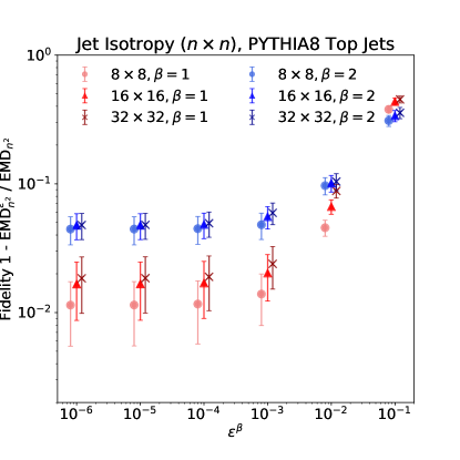
(a)

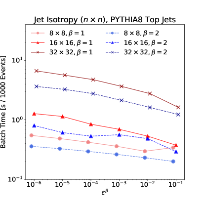
(b)

Figure 3: The (a) fidelity and (b) runtime of Shaper when computing the $n\times n$ jet isotropy, for different values of $\epsilon$, $n$, and $\beta$. The fidelity is defined as the ratio of the Sinkhorn divergence to the “true” Wasserstein metric, as computed using the POT library, across a batch of 1000 events. The runtime is the total time to evaluate the Sinkhorn divergences for the entire 1000 event batch, as computed using a NVIDIA A100. An annealing parameter of $\Delta=0.9$ is used globally.

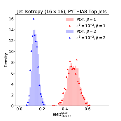
Figure 4: Distributions of the learned $16\times 16$ jet isotropy, for $\beta=1$ (red) and $\beta=2$ (blue), as calculated using the POT library (filled) and Shaper (points) with $\epsilon^{\beta}=10^{-3}$.

In Fig. 3, we show the results of a runtime vs. accuracy study. We compute the jet isotropy of 1000 top jets for several different values of $n$, $\epsilon$, and for $\beta=1$ and $2$. In Fig. 4, we show the learned $16\times 16$ jet isotropies for $\epsilon^{\beta}=10^{-3}$. For this experiment, we use a fixed (conservative) annealing parameter of $\Delta=0.9$. Shaper allows for events to be computed in parallelized batches; we run the entire computation in a single batch on a NVIDIA A100, and report the total runtime of the entire batch.

We see from Fig. 3 that the accuracy of the Sinkhorn divergence, as an estimator for the Wasserstein metric, begins to saturate at $\epsilon^{\beta}=10^{-3}$, and that there is no substantial gain from choosing a smaller $\epsilon$. Picking $\epsilon^{\beta}=10^{-3}$ ensures percent level accuracy for $\beta=1$, and few-percent level accuracy for $\beta=2$, which we can see visually in Fig. 4. Furthermore, for larger values of $n\times n$, the accuracy is mostly independent of $n$. We also observe from Figs. 3 and 4 that Sinkhorn tends to slightly underestimate the Wasserstein metric, which can be understood from the strictly negative $\epsilon^{\beta}$-regulator in Eq. (31). Note that for $n=16$, it takes under 1 second to process 1000 events – this implies it is possible to process millions of events on the order of an hour, with further speedups possible by choosing a more aggressive value for the annealing parameter $\Delta$.

5.3 Benchmarking Optimization: $N$-Subjettiness

We perform a second benchmark investigation using $N$-subjettiness. Unlike the jet isotropy, $N$-subjettiness requires a nontrivial minimization. This allows us to use it to estimate the fidelity of the Shaper algorithm’s optimization step.

It is well known that the ratio $\tau_{32}\equiv\tau_{3}/\tau_{2}$ is a good discriminant between top and QCD jets, as top jets tend to have 3 prongs more often than QCD jets, and thus have lower expected values of $\tau_{32}$ Thaler:2010tr . We compute this ratio for several different values of $\epsilon$ to see if any discrimination power is lost (or gained) in the $\epsilon$-approximation. Within the Shaper framework, the $N$-subjettiness is given by the following manifold of parameterized events:

$$\mathcal{E}_{x_{i},z_{i}}(x)=\sum_{i=1}^{N}z_{i}\,\delta(x-x_{i}),\qquad x_{i}\in\mathcal{X},z_{i}\in\Delta_{N-1}.$$ (40)

As a baseline, we compute $N$-subjettiness using FastJet 3.4.0 with FJcontrib 1.050. The results of this study are shown in Fig. 5a as ROC curves, computed using an NVIDIA A100 GPU. We see that the Sinkhorn approximations have roughly the same discriminatory power as the baseline for $\epsilon\sim 10^{-3}$. In Fig. 6, we show the distributions of $\tau_{32}$ for both datasets computed with FastJet and Shaper with $\epsilon=10^{-3}$, and see good agreement between the two methods. As with the isotropy study in Sec. 5.2, we observe that Shaper tends to slightly underestimate the observable. In order to gauge the impact of float precision on our estimates, we repeat ROC curve calculation using only a CPU, which is shown in Fig. 5b. For values of $\epsilon\ll 10^{-3}$, we see that on the GPU architecture, the performance actually begins to degrade due to the lower machine precision due to the accumulation of floating-point errors during the optimization, while it saturates on the CPU. Therefore, it is recommended to use $\epsilon^{\beta}\sim 10^{-3}$, as this is the most stable compromise between fidelity and machine precision.

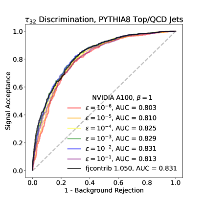
(a)

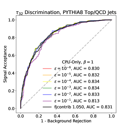
(b)

Figure 5: A ROC curve showing the performance of $\tau_{32}=\tau_{3}/\tau_{2}$ as a discriminator between top (signal) and QCD (background) jets, for several different values of $\epsilon$, as calculated using (a) an NVIDIA A100 and (b) only on CPU. A baseline curve, calculated using the $N$-subjettiness routines in FastJet 3.4.0, is shown in black.

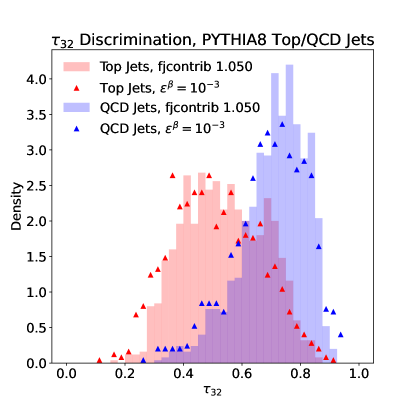
Figure 6: Distributions of the learned $\tau_{32}$, for top jets (red) and QCD jets (blue), as calculated using FastJet 3.4.0 (filled) and Shaper (points) with $\epsilon^{\beta}=10^{-3}$.

5.4 Hearing Gradients

Shaper can be used to not only estimate the shapiness of events, but also take derivatives of the shapiness with respect to the event. As discussed in Sec. 4.3, this is completely automatic, since the gradients with respect to the energy flow are given manifestly by the Kantorovich potentials, allowing us to see precisely how our EMD calculations depend on the energies and positions of particles in an event.

Reading off of Eq. (37), we obtain an expression for the gradient of the EMD with respect to the energy $E_{i}$ of particle $i$:

$$\nabla_{E_{i}}\text{EMD}(\mathcal{E},\mathcal{E}^{\prime}_{\theta}) =F(x_{i}).$$ (41)

If the gradient at particle $i$ is negative, then increasing the energy of that particle will decrease the EMD, making the event more $\mathcal{M}$-like. By adding “ghost” particles to $\mathcal{E}$, one can probe the energy dependence of the EMD from any point in $\mathcal{E}$. Similarly, we can take the gradient the EMD with respect to the position $x_{i}$ of particle $i$:

$$\nabla_{x_{i}}\text{EMD}(\mathcal{E},\mathcal{E}^{\prime}_{\theta}) =E_{i}\nabla_{x_{i}}F(x_{i}).$$ (42)

This gradient (times $-1$) tells us where to move the particle $i$ to decrease the EMD. Both the energy and position gradients answer the question, “If I want to decrease the EMD (make my energy look more like my shape), what should I do to a particle at site $x_{i}$?” Moreover, because of the reparameterization invariance of the energy flow density, the energy and position gradients are both are valid ways to change the EMD: one can either change the energy of particles at the location $x_{i}$, move the particles at $x_{i}$ somewhere else, or some combination of both.

In Figs. 7 and 8, the gradients from Eqs. (41) and (42) are plotted for an example top jet, for the $3$-subjettiness and $16\times 16$,$\beta=1$ jet isotropy, respectively. Using Fig. 7, we can see what parts of the event contribute to the $3$-subjettiness – the three large clusters contribute negatively to the EMD (make the event look more like 3 subjets), while the rest of the event contribute positively to the EMD (makes the event deviate from 3 subjets). Similarly, we see from Fig. 8 that the overdensity of energy at the center of the event makes it less isotropic. In both figures, the vector quiver plot tells us which way particles should “flow” (against) to change the shape.

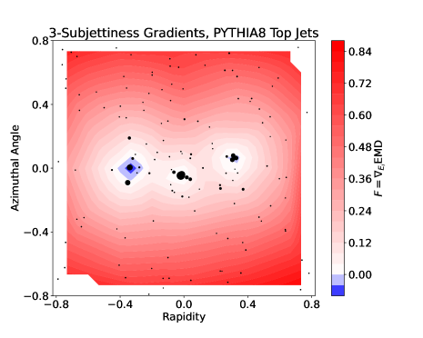
(a)

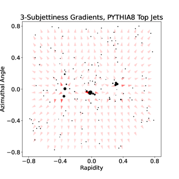
(b)

Figure 7: For an example top jet, (a) gradients of the $3$-subjettiness with respect to the particle weights, $\nabla_{E_{i}}\text{EMD}$, and (b) gradients off the $3$-subjettiness with respect to the particle positions, $\nabla_{x_{i}}\text{EMD}$, are shown. In (a), increasing the particle energy in red regions will increase the $3$-subjettiness (look less like 3 subjets), and increasing particle energy in blue regions will decrease the $3$-subjettiness (look more like 3 subjets). In (b), moving particles along or against the arrows will increase or decrease the $3$-subjettiness, respectively, with the arrow’s shading indicating the relative magnitude of the change.

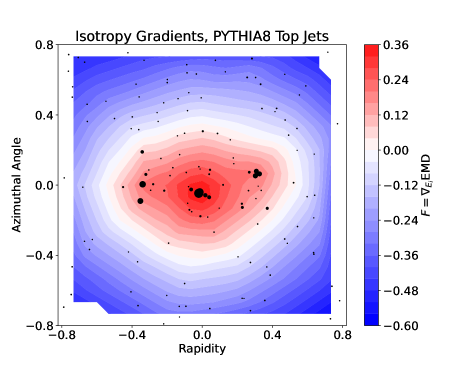
(a)

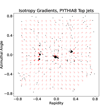
(b)

Figure 8: The same as Fig. 7, but for the $16\times 16$ jet isotropy with $\beta=1$.

There are many potential applications of calculating gradients of a shape with respect to an energy flow. In experimental contexts, for example, one can use the fact that the gradients are practically instantaneous to compute to do easy Gaussian error propagation due to detector-induced uncertainties in particle energies and positions CMS:2016lmd ; ATLAS:2020cli . This avoids having to do expensive re-sampling and recalculation of the event shape. Phenomenologically, these gradients can be used to probe the sensitivity of observables to certain radiation patterns. For example, the sensitivity of an observable to pileup can be measured by taking derivatives with respect to the pileup scale Soyez:2012hv , which can be numerically realized in Shaper, a potential avenue for future work.

5.5 Hearing Jets Ring (and Disk, and Ellipse)

We next use Shaper to realize the custom shape observables defined in Sec. 3.3, starting with some visualizations of these shape observables on an example event.

The three base observables we consider are the ringiness, diskiness, and ellipsiness, as defined in Sec. 3.3. We calculate the shape observables $N\times\mathcal{O}$ (the $N$-ringiness, the $N$-diskiness, and $N$-ellipsiness) and $N\times\mathcal{O}^{\tau}$ (the $N$-(ring$+$point)iness, the $N$-(disk$+$point)iness, and $N$-(ellipse$+$point)iness), as defined in Sec. 3.3 with $\beta=1$. We also consider, for comparison, the $N$-subjettiness, $\tau_{N}$, as defined in Eq. (40). We use Shaper to evaluate all of these shape observables on a single of top jet event from our dataset, restricted to $m_{J}\in[145,205]\,\text{GeV}$, though without any pileup contamination. Each extended shape is sampled with $100$ points, with $\epsilon=10^{-3}$ and $\Delta=0.9$.

Geometric visualizations of each of the 21 event shapes, as evaluated on an example top jet, can be found in Figs. 9, 10, 11, and 12. From these visualizations, we note some interesting qualitative features of these shape observables. First, the point variants of each shape correspond more closely to clusters of energy. For example, while the $N=3$ uniform rings (Fig. 10), disks (Fig. 11), or ellipses (Fig. 12) do not necessarily capture the regions of highest energy, the point variants of each shape align very well with the $N$-subjettinesses of Fig. 9. Correspondingly, the EMD’s of the shapes are significantly reduced for the point variants – this suggests that this event in particular is not well modeled by uniform radiation profiles, but rather looks more like localized spikes with radiation clouds around them. Moreover, we can see that circular radiation clouds do not model the event as well as elliptical ones – this is reflected in the $N$-ellipsiness in Fig. 12, which learns extremely eccentric line-like structures in an attempt to best model the event, which results in lower EMD’s than the corresponding $N$-diskinesses in Fig. 11. We also note that the $N$-subjettiness and the point shape variants all qualitatively find the same jet centers, suggesting that these shapes can be treated as perturbations to $N$-subjettiness.

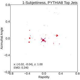
(a)

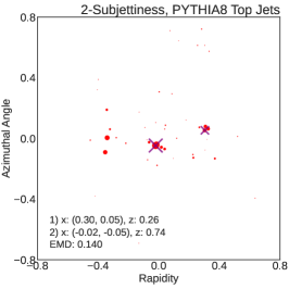
(b)

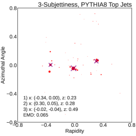
(c)

Figure 9: The (a) 1-, (b) 2-, and (c) 3-subjettiness of an example top jet event. Subjets are represented by a purple “$\times$”, with size proportional to the subjet’s energy weight.

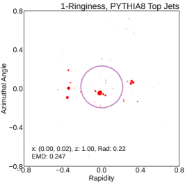
(a)

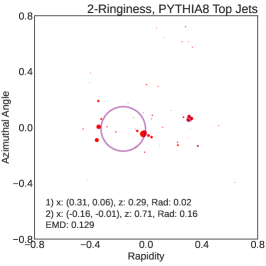
(b)

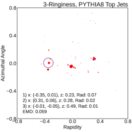
(c)

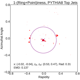
(d)

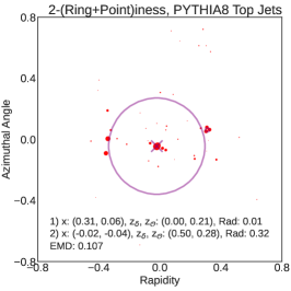
(e)

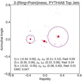
(f)

Figure 10: Top row: the (a) 1-, (b) 2-, and (c) 3-ringiness of an example top jet event. Bottom row: the (d) 1-, (e) 2-, and (f) 3-(ring$+$point)iness of the same top jet event. The point is represented by a “$\times$”, with size proportional to its energy weight.

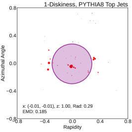
(a)

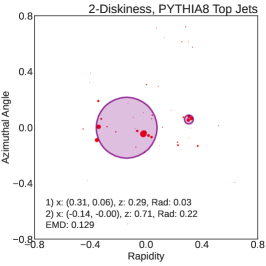
(b)

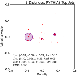
(c)

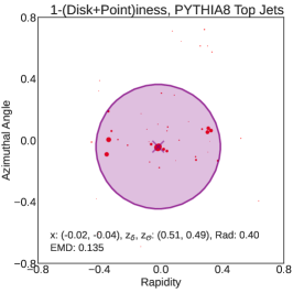
(d)

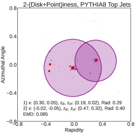
(e)

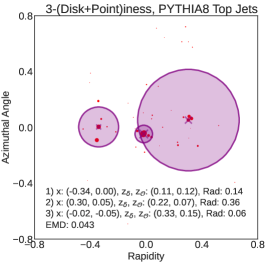
(f)

Figure 11: Top row: the (a) 1-, (b) 2-, and (c) 3-diskiness of an example top jet event. Bottom row: the (d) 1-, (e) 2-, and (f) 3-(disk$+$point)iness of the same top jet event. The point is represented by a “$\times$”, with size proportional to its energy weight.

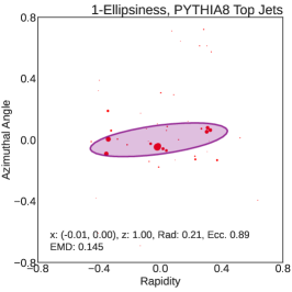
(a)

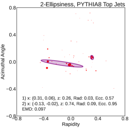
(b)

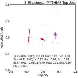
(c)

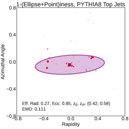
(d)

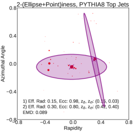
(e)

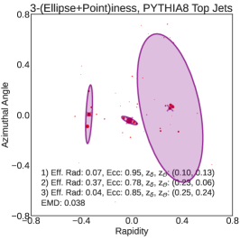
(f)

Figure 12: Top row: the (a) 1-, (b) 2-, and (c) 3-ellipsiness of an example top jet event. Bottom row: the (d) 1-, (e) 2-, and (f) 3-(ellipse$+$point)iness of the same top jet event. The point is represented by a “$\times$”, with size proportional to its energy weight. The effective radius of the ellipses are given by the geometric mean of the two axes, $\sqrt{ab}$.

5.6 Shapiness and Shape Parameters

Continuing the discussion in Sec. 5.5, we now use Shaper to compute distributions of these shape observables on a large sample of top and QCD jets, restricted to $m_{J}\in[145,205]\,\text{GeV}$, though without any pileup contamination. In particular, we show the utility of both the shapiness $\mathcal{O}(\mathcal{E})$ and the shape parameters $\theta(\mathcal{E})$ in describing the geometry of jets.

For each histogram in this section, we calculate an AUC score, showing the efficacy of a cut on that observable as a top/QCD discriminant. Note that these AUCs are for cuts on a single feature – the discrimination power can in principle be improved by transforming these features and combining many features per jet.

As a representative sample of the “shapiness” observable, we plot the $N$-ellipsiness and $N$-(ellipse$+$point)iness of our top and QCD jet samples in Fig. 13. The EMD distributions for the ring and disk variants are qualitatively similar to the ellipse, and thus our discussion of these distributions carry over to them. We notice that the $N$-(ellipse$+$point)iness is not much lower than the corresponding $N$-ellipsiness, indicating that (at least in the absence of pileup), subjets can indeed be approximated as roughly uniform. In the test event visualization in Fig. 12, we can see qualitatively that the found ellipses have roughly the same center, comparing the $N$-ellipsiness and its corresponding point variant. We also note that the EMD decreases with $N$, as expected.

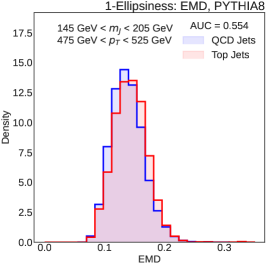
(a)

(b)

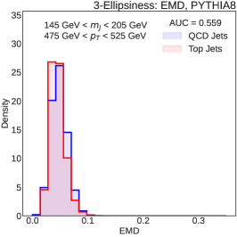
(c)

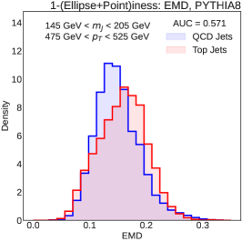
(d)

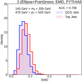
(e)

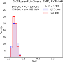
(f)

Figure 13: Distributions of the learned (a,d) 1-, (b,e) 2-, and (c,f) 3-ellipsiness (top row) and (ellipse$+$point)iness (bottom row) of the top (red) and QCD (blue) jet sample.

In Fig. 14, we show the ratio of the $N=3$ shapiness to the $N=2$ shapiness for each class of shape observable. For $N$-subjettiness, which we show for comparison, this is the classic observable $\tau_{32}$, which is known to be a good top vs. QCD jet discriminant Thaler:2010tr . First, we observe that the uniform ring, disk, and ellipse observable, along with the point variants, each have an AUC of approximately 0.75, which is still considerably less than $\tau_{32}$’s AUC of 0.825. One should expect that, using just the EMD alone, a more complexly parameterized shape should have a lower AUC than a simpler shape. In the extreme case, where the parameterization is flexible enough to reproduce any event in the dataset, the EMD will always be zero and have no discriminatory power. However, this is not the end of the story – shape observables also include their learned parameters, and this information also contains multivariate discriminatory power. For the hypothetical infinitely flexible shape, the parameters contain the full event information even though the EMD is zero, and thus the combination of the shapiness and shape parameters together contain more information (and thus more discriminatory power) than just a simpler shape. We leave a full multivariate analysis of shape parameters for jet classification for potential future work.

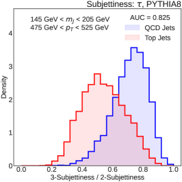
(a)

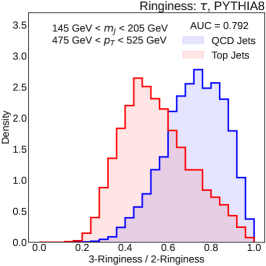
(b)

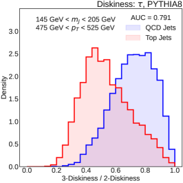
(c)

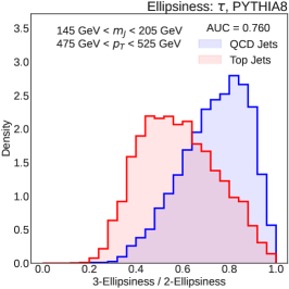
(d)

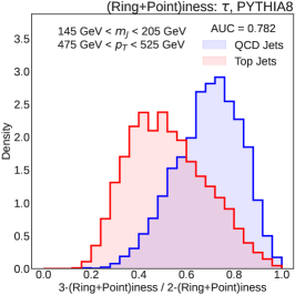
(e)

(f)

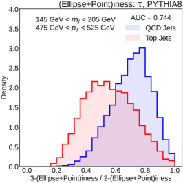
(g)

Figure 14: Top row: Distributions of the $N=3$ to $N=2$ ratio of the (a) $N$-subjettiness of the top (red) and QCD (blue) jet sample. Middle row: The same ratio, but for the $N$- (b) ringiness, (c) diskiness, and (d) ellipsiness. Bottom row: The same, but for the $N$- (e) (ring$+$point)iness, (f) (disk$+$point)iness, and (g) (ellipse$+$point)iness.

We now move on to analyze the learned shape parameters themselves. In Fig. 15, the learned radius parameters of the $N=1$ shapes are shown. Considering the $1$-(disk$+$point)iness and $1$-(ellipse$+$point)iness, which as discussed earlier, we can think of as a “jet algorithm” looking for soft clusters of radius $R$ with collinear radiation inside, we see that both learn an average radius of approximately $R=0.4$, which is approximately half the radius of the original AK8 jet. One can think of the uniformity condition as imposing an radius effective cutoff. If one assumes that the energy density falls to zero with distance from the jet center, then there is some critical radius for which any larger uniform shape is an increasingly worse approximation, and in principle this critical radius can be computed in perturbative QCD.

For the point shape variants of the disk and ellipse, we note that there is only a small difference between the top and QCD jets – that is to say, the soft component of a top jet is about as “wide” as the soft component of a QCD jet, as seen by disks and ellipses. However, as top jets tend to have their energy distributed across 3 prongs, rather than 1 prong as in QCD jets, we should expect clusters of radiation away from the central one for top jets. Since rings are thin, we should expect rings to be able to better capture these localized prongs than area-filling disks and ellipses, which can be visualized in Fig. 10. This is especially apparent in Fig. 15d for the $1$-(ring$+$point)iness shape, where top jets are significantly larger than QCD jets. Interestingly, we note a spike at $R=0$ in all of these distributions. This means that Shaper has determined that the best shape for these events is in fact point-like, and reduces to the $N$-subjettiness. This spike is reduced for the ellipse shapes, which implies that there are events better modeled by either an eccentric ellipse or a point rather than a uniform disk.

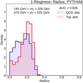
(a)

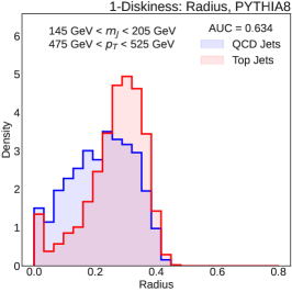
(b)

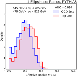
(c)

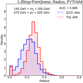
(d)

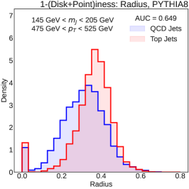
(e)

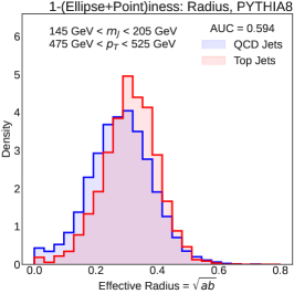
(f)

Figure 15: Top row: distributions of the learned radius parameter of the 1- (a) ringiness, (b) diskiness, and (c) ellipsiness of the top (red) and QCD (blue) jet sample. Bottom row: the radius parameter of the 1- (d) (ring$+$point)iness, (e) (disk$+$point)iness, and (f) (ellipse$+$point)iness of the same samples. For the ellipse, the effective radius is given by the geometric mean of the two axes.

As a last example of the information that shape observables and shape parameters can extract, we look at the learned eccentricity of ellipses. In Fig. 16, we show the minimum eccentricity across the $N$ ellipses for the $1$-, $2$-, and $3$- ellipsiness and (ellipse$+$point)iness for our top and QCD jet datasets, where the eccentricity is given by $\sqrt{1-\min(a,b)/\max(a,b)}$. We can immediately see that a value of $\min(e)=0$ is rare – our jets are much better described by ellipses than they are described by disks. With increasing $N$, the distributions of $\min(e)$ tend to shift leftwards for both the top and QCD jet samples. This indicates that the $N$-’th ellipse, which probes more substructure than the $(N-1$)-’th ellipse, is often less eccentric.

The eccentricity distributions for top jets are slightly different from QCD jets. This is a nontrivial result; top jets and QCD jets have very different prong structures (as demonstrated in Fig. 14), so the angular distribution of radiation in the rapidity-azimuth plane is less circular for top jets than QCD jets. Thus, jet eccentricity could be used as a discriminant.

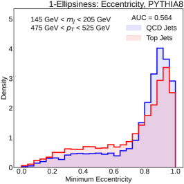
(a)

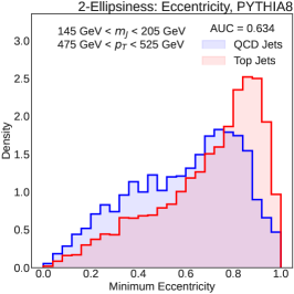
(b)

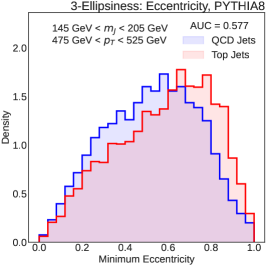
(c)

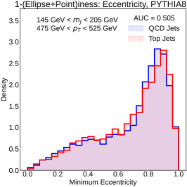
(d)

(e)

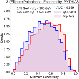
(f)

Figure 16: Distributions of the learned minimum eccentricities for (a,d) 1-, (b,e) 2-, and (c,f) 3-ellipsiness (top row) and (ellipse$+$point)iness (bottom row) of the top (red) and QCD (blue) jet sample.

The above plots show just a few examples of the information that can be extracted using generalized shape observables. It is important to emphasize there is much more information beyond what we have shown here available for analysis, such as the learned weights of the points versus uniform shapes, the radii of shapes beyond the leading jet, and so on. This is to say nothing of the multivariate information contained in the correlations between the EMDs and shape parameters, both within the same shape and between different shapes. We leave a full quantitative study of the information contained within shapes for potential future work.

5.7 Pileup-Mitigating Shapes

Finally, we show a use case for shape observable composition by applying our custom shape observables to the task of pileup mitigation. We consider the top jet mass spectrum as an example, which is sharply peaked near $m_{\rm top}^{2}\approx(175\,\text{GeV})^{2}$. In our modified dataset, jets are contaminated with uniform pileup radiation, which significantly biases and smears the top mass peak. There exist many techniques to “groom” away extra contamination, such as area subtraction and soft drop Cacciari_2008 ; Cacciari_2008_2 ; Soyez:2012hv ; Larkoski:2014wba ; Dasgupta_2013 , but these techniques often have external hyperparamters characterizing the contamination density (such as $z_{\rm cut}$ in soft drop).

In order to mitigate this bias even when the contamination density is unknown, we propose to build shapes that factorize the event into a uniform component, $\mathcal{U}$, and a structure component, $\mathcal{E}$. As described in Sec. 3.3.5, we accomplish this by building observables of the form:

$$\mathcal{O}^{\mathcal{I}}_{i}=\mathcal{O}_{i}\oplus\mathcal{I},$$ (43)

where $\mathcal{O}_{i}$ is any shape observable and $\mathcal{I}$ is the jet isotropy. We can then use the energy flow associated to $\mathcal{O}_{i}$ to calculate a “pileup-corrected” mass, discarding the energy flow associated to $\mathcal{I}$. The weight $z_{2}$ associated with $\mathcal{I}$ is then an estimate of the fraction of event energy due to pileup – the contamination density is an extracted observable, not an assumed hyperparameter!

For this study, we consider $\mathcal{O}_{i}^{\mathcal{I}}$, where $\mathcal{O}_{i}$ is either the 3-subjettiness or the 3-(disk$+$point)iness, motivated by the 3-prong nature of top jets. We also consider the uncorrected observables, $\mathcal{O}_{i}$, without the uniform background for comparison. For each observable, the “shape-jet mass” $m_{J}$ is calculated as the sum as the (massless) four vectors of particles comprising the shape. This can be numerically approximated by sampling the disk with 200 particles. To calibrate the shape-jet masses, we calculate the shape-jet mass on top jets without the addition of pileup for each observable. In Fig. 17a, we plot the shape-jet mass corresponding to each observable as evaluated on top jets. Each observable slightly undershoots the top mass peak – the exact discrepancies are given in Table 5. These values are used to shift the means of each shape-jet mass curve to the right for the remainder of this study, such that the means give the truth mean top mass when evaluated on uncontaminated jets.

In Fig. 17b, we show the result of an empirical study using our pileup-mitigating shapes on our pileup-contaminated top jet sample. We also plot, for comparison, the mass corresponding to the uncorrected observables $\mathcal{O}_{i}$, with no uniform background. These distributions are all calibrated using the values in Table 5. We see clearly that the two pileup-mitigating shapes indeed remove a significant amount of bias due to pileup, and bring $m_{\rm jet}$ much closer to $m_{\rm top}$, suggesting that this is a viable strategy for pileup removal. Note, interestingly, that the distribution for the uncorrected 3-(disk$+$point)iness jet mass is similar to the uncorrected jet mass – this is because to best approximate the entire event, disks will grow large in an attempt to capture all of the pileup, since the disks themselves are also uniform radiation patterns.

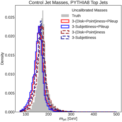
(a)

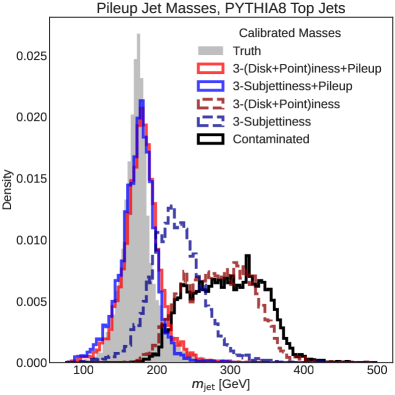
(b)

Figure 17: The shape-jet mass for several different choices of shape observable, evaluated on (a) top jets without pileup, used to derive the calibration, and (b) top jets with pileup, calibrated using Table 5. Two different shape observables are used – the 3-jettiness in blue and 3-(disk$+$point)iness in red. For each shape observable, the ordinary version is plotted with dark dashed lines while the pileup-mitigating variant is plotted with bright solid lines.

Observable	Bias [GeV]
3-(Disk$+$Point)iness$+$Pileup	$-18.7$
3-Subjettiness$+$Pileup	$-23.1$
3-(Disk$+$Point)iness	$-5.5$
3-Subjettiness	$-12.5$

Table 5: The difference between the mean shape-jet mass and the mean of the truth top jet distribution in Fig. 17a, for each of the four observables under consideration. These are used to calibrate the calculated mass distributions for each shape.

In Fig. 18a, we show the distribution of extracted pileup energy fraction values, corresponding to the $z_{2}$ shape parameter. We see that there is qualitative agreement between the extracted pileup energy fractions and the true one, though the shapes tend to overestimate the pileup density slightly. This is consistent with Fig. 17b, where the shapes slightly underestimate the top mass without the calibration. In Fig. 18b, we use $z_{2}$ to compute the value of the extracted mass bias $\Delta\hat{m}^{2}_{\rm PU}=m^{2}_{\rm jet}-\hat{m}^{2}_{\rm top}(z_{2})$, compared to the “true” mass bias obtained by comparing the jet mass before and after contamination. To approximate the resolution of our estimator, we take $\hat{\sigma}^{2}={\rm Var}\left[\sqrt{\hat{m}^{2}_{\rm PU}}-\sqrt{m^{2}_{\rm PU}}\right]$ as the average Gaussian uncertainty. We can see that both pileup-mitigating observables estimate the pileup mass bias correctly on average, and that the 3-(disk$+$point)iness$+$pileup has a slightly better resolution than the 3-subjetiness$+$pileup, which is to be expected as the former has more freedom to better capture features of jets.

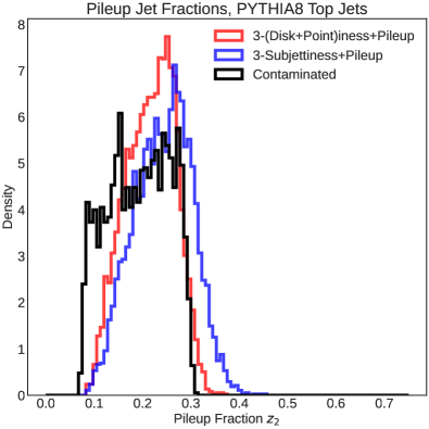
(a)

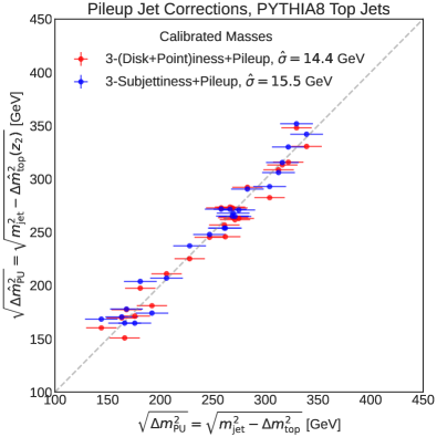
(b)

Figure 18: (a) The learned pileup fractions $z_{2}$ for the 3-jettiness in blue and 3-(disk$+$point)iness in red. The actual fraction of energy due to pileup is in black. (b) The mass corrections to the top mass due to pileup, for the 3-jettiness in blue and 3-(disk$+$point)iness in red. On the $x$-axis, the change in jet mass $(\Delta m^{2}_{\rm PU})^{1/2}$ before and after contamination is plotted. On the $y$-axis, the value of $(\Delta\hat{m}^{2}_{\rm PU})^{1/2}$ as extracted from the corrected top mass is plotted for a small test set. As a proxy for the resolution of the estimate, we take $\hat{\sigma}$ to be the standard deviation of the residuals.

6 Conclusions and Outlook

In this work, we generalized the notion of event and jet shapes into shape observables, which are a wide class of observables that can probe the geometric structure of collider events. We introduced a natural measure-theoretic language for describing events as energy flows, which encodes properties such as IRC safety as inherent topological information. Using this construction, we showed that the Wasserstein metric arises naturally from the requirement of geometric faithfulness. This post-hoc justifies its past use to define observables, IRC safety, and geometry on the space of events Komiske_2019 ; 2020 ; Cesarotti:2020hwb ; Cai:2021hnn .

We showcased how to define arbitrary shape observables, which can be specified solely by parameterizing the manifold of shapes one wants to fit to. Importantly, we can extract both the “shapiness” value (how much the event looks like the shape) and the “shape parameters” (which shape is the best fit). This is a very intuitive picture – if one wants to ask how “ellipsy” a jet is, for example, all one needs to do is parameterize the space of ellipses to define the ellipsiness observable. The Shaper framework makes it easy to build new shape observables and evaluate them on events. It leverages the Sinkhorn approximation of the Wasserstein metric to enable fast, parallelizable, and differentiable $\epsilon$-approximations of shape observables.

With the Shaper framework in place, the natural question arises: Which shapes should we study? We introduced a few examples of shapes motivated by jet substructure, including rings, disks, and ellipses. Using the Shaper prescription, it is easy to modify these shapes to probe additional jet structures, by including $\delta$-functions to capture collinear radiation or uniform backgrounds to capture pileup. Our empirical studies showed how these custom observables might serve as an effective and simple pileup mitigation strategy in the study of top jets, where the amount of pileup does not need to be assumed beforehand. Many further analyses are possible: for example, in heavy quark decays, collinear bremsstrahlung is suppressed (the so-called “dead-cone effect” Dokshitzer:1991fc ; Dokshitzer:1991fd ; PhysRevLett.69.3025 ), leading to ring-like or annulus-like, rather than point-like, jets. Moreover, the ability to take derivatives with respect to entire events could allow one to compute observable sensitivities, such as pileup sensitivity Soyez:2012hv . The list of observables we have provided is certainly non-exhaustive, and we hope that the Shaper framework can be used by the community to explore a wide range of brand new observables.

While Shaper can be used to analyze any shape observable, and thus has broad generality, it is not necessarily the fastest way to compute or approximate any specific observable. For example, much faster, exact algorithms for computing $N$-jettiness and related observables are available in the FastJet Cacciari:2011ma package, which make use of the fact that the double optimization in Eq. (18) can be simplified. Most of the new observables we have defined appear to be irreducible, though, making their analysis and theoretical treatment complicated. In principle, this class of observables is perturbatively calculable in QCD, at least numerically. We anticipate that these generalized shapes might provide a useful groundwork for further theoretical studies of QCD distributions.

Code and Data

The code for the general-use Shaper framework can be found at https://github.com/rikab/SHAPER, along with installation instructions. This directory also contains the analysis code for the top/QCD plots in Sec. 5. In this directory is also a tutorialized example notebook, showing how to use the Shaper framework.

Our dataset is a modified version of the top/QCD jet benchmark dataset described in Refs. Butter:2017cot ; Kasieczka:2019dbj . The original version of this dataset can be found at https://desycloud.desy.de/index.php/s/llbX3zpLhazgPJ6.

Appendix A Energy Flows as Measures

In this appendix, we review aspects of measure theory and topology related to energy flows, as introduced in Sec. 2.2. To begin, we define a measure:

Definition 4.

Given a set $\mathcal{X}$ and a $\sigma$-algebra on $\mathcal{X}$ denoted $\sigma(\mathcal{X})$, a (positive) measure $\mathcal{E}$ over $\sigma(\mathcal{X})$ is a function $\mathcal{E}:\sigma(\mathcal{X})\to\mathbb{R}$ satisfying:

• Non-Negativity: For all $X\in\sigma(\mathcal{X})$, we have $\mathcal{E}(X)\geq 0$.

• Null Set: For the empty set, we have $\mathcal{E}(\emptyset)=0$.

• Additivity: For a (countable) collection of disjoint sets $X_{i}\in\sigma(\mathcal{X})$, we have:

  $$\mathcal{E}\left(\bigcup_{i}X_{i}\right)=\sum_{i}\mathcal{E}(X_{i}).$$ (44)

If, additionally, we have $\mathcal{E}(\mathcal{X})=1$, we say $\mathcal{E}$ is a probability measure.

Associating energy flows with measures is very natural: an energy flow answers the question “How much energy did I detect in the calorimeters located within the subregion $X$ of my detector $\mathcal{X}$?”, and this answer satisfies all of the above properties. We refer to $\mathcal{E}(X)$ as the energy flow, whereas we call the object

$$\mathcal{E}(x)=\sum_{i}E_{i}\delta(x-x_{i})$$ (45)

as the energy flow density or measure density. This language (while different from Ref. 2020 ) is natural, since integrating over Eq. (45) yields the energy flow:

$$\mathcal{E}(X)=\int_{X}dx\,\mathcal{E}(x).$$ (46)

Under this definition, the energy flow is independent of the choice of coordinates $x$ used on $\mathcal{X}$, unlike the energy flow density. In particular, the form of energy flow is completely invariant under exactly 0-energy emissions or exactly collinear splittings, and additionally is also invariant under particle relabellings. Throughout this paper, we restrict ourselves to measures that can be written as the integral of a well-behaved associated density, which is the case for all physically realized energy flows. We refer to measures whose density is a finite sum of weighted $\delta$-functions as atomic measures.

Measures can be used to formalize what we mean by integration. We begin by defining $\expectationvalue{\mathcal{E},\phi}$ as the integral of an integrable function $\phi:\mathcal{X}\to\mathbb{R}$ against an energy flow $\mathcal{E}$. Assuming coordinates $x$ on $\mathcal{X}$, we define this quantity as the ordinary integral over the associated energy flow density:

$$\expectationvalue{\mathcal{E},\phi}\equiv\int_{\mathcal{X}}dx\,\mathcal{E}(x)\,\phi(x).$$ (47)

In the special case where $\mathcal{E}$ is a probability measure, this quantity is the expectation value $\mathbb{E}_{X\sim\mathcal{E}}\left[\phi(X)\right]$ of the random variable $\phi(X)$ sampled over $\mathcal{E}$. The notation $\expectationvalue{\mathcal{E},\phi}$ highlights the inner product structure of a measure $\mathcal{E}$ “acting” on the space of functions on $\mathcal{X}$. Notably, this inner product is bilinear – though when considering positive measures, one must be careful to not produce energy flows where the energy is anywhere negative, as these are nonphysical.

Next, we discuss the important topological features of measures. First, we define weak* convergence (also sometimes referred to as convergence in law) of a sequence of measures:

Definition 5.

A sequence of measures $\mathcal{E}_{n}$ converges with respect to the weak* topology to a measure $\mathcal{E}$, which we denote $\mathcal{E}_{n}\to\mathcal{E}$, if for any continuous test function $\phi$ on $\mathcal{X}$, the sequence of real numbers $\expectationvalue{\mathcal{E}_{n},\phi}$ converges to the real number $\expectationvalue{\mathcal{E},\phi}$.

That is, we say a sequence of measures converges if every single expectation value converges. Associated to this definition of convergence is the weak* topology, which is the (weakest) topology for which the map $\expectationvalue{\cdot,\phi}$ is considered continuous for all continuous $\phi$. Note that this definition does not make use of any metric on measures; it simply inherits the metric and topological structure of the real numbers. Building off of this, we can now define what it means for any function on energy flows to be continuous:

Definition 6.

A function $F$ on the space of positive measures is continuous with respect to the weak* topology if, for every convergent sequence of measures $\mathcal{E}_{n}\to\mathcal{E}$, the sequence $F(\mathcal{E}_{n})$ converges to $F(\mathcal{E})$.

Continuity is a very powerful tool for dealing with energy flows. First, it immediately implies that continuous measures can be arbitrarily well approximated by atomic measures with an increasing number of samples. Moreover, if a function $F$ on measures is continuous with respect to the weak* topology, this further implies it is only necessary to specify how $F$ acts on atomic measures, since the action on all other measures is fixed by weak* continuity.

Intuitively, weak continuity captures the idea that a continuous distribution is well approximated by a discrete one with “enough samples” – as the number of sample increases, we approach the continuous one. Note, however, we have not yet defined what it means for two energy flows to be “close” to each other, so we cannot yet describe what happens to functions under small energy flow perturbations. This requires a metric on the space of energy flows that respects the weak* topology, which as argued in Sec. 2 and further justified in App. B, can be taken to be the Wasserstein metric.

We finally introduce one last piece of notation. For any two energy flows $\mathcal{E}_{1}$ and $\mathcal{E}_{2}$, the joint energy flow $\mathcal{E}=\mathcal{E}_{1}\otimes\mathcal{E}_{2}$ is the energy flow satisfying for any sets $X,Y\subseteq\mathcal{X}$:

$$\mathcal{E}(X,Y)=\int_{X\times Y}dx\,dy\,\mathcal{E}_{1}(x)\,\mathcal{E}_{2}(y).$$ (48)

The energy flows $\mathcal{E}_{1}$ and $\mathcal{E}_{2}$ are referred to as the marginals of $\mathcal{E}$. They can be written as $\mathcal{E}_{1}(X)=\mathcal{E}(X,\mathcal{X})$ and $\mathcal{E}_{2}(Y)=\mathcal{E}(\mathcal{X},Y)$, with densities $\mathcal{E}_{1}(x)=\int_{\mathcal{X}}dy\,\mathcal{E}(x,y)$ and $\mathcal{E}_{2}(y)=\int_{\mathcal{X}}dx\,\mathcal{E}(x,y)$ respectively.

Appendix B Constructing the Wasserstein Metric

In Sec. 2.1, we proposed to write event and jet shapes $\mathcal{O}_{\mathcal{M}}$ using some universal loss function $\mathcal{L}$ on energy flows, and in Sec. 2.3, we showed that IRC safety implies that must $\mathcal{L}$ must be weakly continuous. Then, in Sec. 2.4, we claimed that the condition of faithfully lifting the ground metric means that $\mathcal{L}$ must be the Wasserstein metric, and showed examples of how similar metrics do not satisfy this property. In this appendix, we show how the Wasserstein metric arrives constructively. First, in App. B.1, we briefly review the properties we use to construct $\mathcal{L}$, before outlining the construction in App. B.2.

B.1 Shaping Up the Loss

To start, we list the properties we would like the universal loss function $\mathcal{L}$ to satisfy. First, we would like $\mathcal{L}$ to be a proper metric on the space of energy flows, which implies the following usual properties of metrics:

1. Finiteness: We require that $\mathcal{L}$ is finite, even when evaluated on atomic measures. This immediately rules out the KL divergence kullback1951information and its variants, including log-likelihoods, used in Ref. Mackey:2015hwa to define “fuzzy jet” observables. These functions are only finite on continuous measures with support almost everywhere.

2. Positivity and Closure: We require that $\mathcal{L}(\mathcal{E},\mathcal{E}^{\prime})\geq 0$. Moreover, we require that $\mathcal{L}(\mathcal{E},\mathcal{E}^{\prime})=0$ if and only if $\mathcal{E}=\mathcal{E}^{\prime}$. This captures the notion of the “optimal shape” as discussed in Sec. 2.1.

3. Symmetry: We require that $\mathcal{L}(\mathcal{E},\mathcal{E}^{\prime})=\mathcal{L}(\mathcal{E}^{\prime},\mathcal{E})$. This is to say, if the energy flow $\mathcal{E}$ looks like $\mathcal{E}^{\prime}$, then the energy flow $\mathcal{E}^{\prime}$ looks like $\mathcal{E}$ as well.

We will not specifically require the triangle inequality, as we never use it throughout this work. Of course, the Wasserstein metric does indeed satisfy the triangle inequality when the appropriate powers of $1/\beta$ are included, making it a proper metric.

Not only is $\mathcal{L}$ a metric, but it must be continuous to the weak* topology to be IRC safe, as established in Sec. 2.3:

1. Weak Contintuity/IRC Safety: We require that $\mathcal{L}$ is weakly continuous in both of its arguments. This not only allows for continuous energy flows to be arbitrarily well approximated by atomic energy flows, but heavily constrains the energy- and position- dependence of $\mathcal{L}$.

Finally, as discussed in Sec. 2.4, we demand that $\mathcal{L}$ faithfully lifts the ground metric. This allows the space of events to inherit the geometry of the ground metric space with no distortions or warping:

1. Faithfully Lifts the Ground Metric: We require that if $\mathcal{E}$ and $\mathcal{E}^{\prime}$ are atomic measures with a single normalized particle at positions $x$ and $y$ respectively, then $\mathcal{L}(\mathcal{E},\mathcal{E}^{\prime})$ is proportional to $d(x,y)^{\beta}$, where $\beta$ is some fixed positive power.

   Moreover, we require that $\mathcal{L}$ faithfully lifts the ground metric. For any measure $\mathcal{E}$, we can “translate” the measure by $t$ to $\mathcal{E}_{t}$, defined by the density $\mathcal{E}(x-t)$. We then require that $\mathcal{L}(\mathcal{E},\mathcal{E}_{t})$ is proportional to $d(0,t)^{\beta}$.

If the ground metric is translationally invariant, which is the case for Euclidean metrics, property 5 implies that $\mathcal{L}$ must also be translationally invariant – if both $\mathcal{E}$ and $\mathcal{E}^{\prime}$ are translated by a vector $t$, the metric distance between them is unchanged.

B.2 Why Wassterstein?

Having defined the properties we would like our universal loss function to satisfy, we can now finally construct $\mathcal{L}(\mathcal{E},\mathcal{E}^{\prime})$.

To begin, weak continuity allows us to drastically simplify the problem. Continuous energy flows may be approximated arbitrarily well by atomic energy flows, and thus it suffices to build our function only on atomic energy flows. This allows us to argue that $\mathcal{L}$ can only depends on single powers of the distance $d(x,y)^{\beta}$. In particular, lifting the ground metric (though not necessarily faithfully, yet) forbids terms of the form $d(x,y)^{\beta}d(x^{\prime},y^{\prime})^{\beta}$ or other higher-order distance correlations, since in the single-particle case this would result in losses of the form $d^{\beta_{1}}+d^{\beta_{2}}+...$ with several differing exponents. This implies the following form for $\mathcal{L}$ when evaluated on uniform atomic flows $\mathcal{E}\sim\sum_{i}\delta_{x_{i}}$ and $\mathcal{E}^{\prime}\sim\sum_{j}\delta_{y_{j}}$:

$$\mathcal{L}(\mathcal{E},\mathcal{E}^{\prime}) =\Pi\left(\sum_{i,j}\pi_{ij}\,d(x_{i},y_{j})^{\beta}\right)$$

$$+K\left(\sum_{i_{1},i_{2}}k_{i_{1}i_{2}}\,d(x_{i_{1}},x_{i_{2}})^{\beta}\right)+K\left(\sum_{j_{1},j_{2}}k_{j_{1}j_{2}}\,d(y_{j_{1}},y_{j_{2}})^{\beta}\right)$$

$$+F\left(\sum_{i}f_{i}\,d(x_{i},g(x_{i}))^{\beta}\right)+F\left(\sum_{j}f_{j}\,d(\tilde{g}(y_{j}),y_{j})^{\beta}\right),$$ (49)

where $\Pi$, $K$, and $F$ are universal functions, $\pi$, $k$, and $f$ are coefficients that implicitly depend on the two measures, and $g$ is a function from the domain of $\mathcal{E}$ to the domain of $\mathcal{E}^{\prime}$ (and vice-versa for $\tilde{g}$). Note that this form is symmetric under swapping $\mathcal{E}$ and $\mathcal{E}^{\prime}$. Without loss of generality, $k_{ii^{\prime}}$ can be chosen to be a symmetric traceless matrix.

Still considering the single particle case, lifting the ground metric also implies that the functions $\Pi$ and $F$ must be linear functions (though the single particle case provides no information about $K$), as to reproduce the desired $d(x,y)^{\beta}$ behavior. Moreover, to still maintain only terms proportional to $d^{\beta}$ even in the multiparticle case, $K$ must also be linear. This linearity means that we can combine the arguments of each of the $\Pi$, $K$, and $F$ functions.

Recall that energy flows are additive objects, and the energy flows defined by the densities $\mathcal{E}=(E_{1}+E_{2})\delta_{x}$ and $\mathcal{E}=E_{1}\delta_{x}+E_{2}\delta_{x}$ must be identical. This implies that each term of the terms in Eq. (49) must be individually linear in the energy weights of $\mathcal{E}$ and $\mathcal{E}^{\prime}$, respectively. This implies the following constraints, up to an overall proportionality factor:

$$\sum_{i}\pi_{ij} =E_{j}^{\prime},$$ (50)

$$\sum_{j}\pi_{ij} =E_{i},$$ (51)

$$\sum_{i_{1}}k_{i_{1}i_{2}} =E_{i_{2}}, \sum_{i_{2}}k_{i_{1}i_{2}} =E_{i_{1}},$$ (52)

$$\sum_{j_{1}}k_{j_{1}j_{2}} =E_{j_{2}}^{\prime}, \sum_{j_{2}}k_{j_{1}j_{2}} =E_{j_{1}}^{\prime},$$ (53)

$$f_{i} =E_{i}, f_{j} =E_{j}^{\prime}$$ (54)

Now, consider the two particle case, as in Sec. 2.4, and define the energy flows for vectors $a$ and $t$:

$$\mathcal{E}(x) \sim\frac{1}{2}\delta_{0}+\frac{1}{2}\delta_{a},$$ (55)

$$\mathcal{E}^{\prime}(x) \sim\frac{1}{2}\delta_{t}+\frac{1}{2}\delta_{a+t}.$$ (56)

When $t\to 0$, the two energy flows are the same, and when $a\to 0$, the energy flows reduce to the single particle case. Evaluating Eq. (49), we obtain:

$$\mathcal{L}(\mathcal{E},\mathcal{E}^{\prime}) =\Pi\left(\pi_{1_{x}1_{y}}d(0,t)^{\beta}+\pi_{1_{x}2_{y}}d(0,a+t)^{\beta}+\pi_{1_{x}1_{y}}d(a,t)^{\beta}+\pi_{2_{x}2_{y}}d(a,a+t)^{\beta}\right)$$

$$+K\left(2k_{1_{x}2_{x}}d(0,a)^{\beta}+2k_{1_{y}2_{y}}d(t,a+t)^{\beta}\right)$$

$$+\frac{1}{2}F\left(d(0,g(0))^{\beta}+d(a,g(a))^{\beta}+d(\tilde{g}(t),t)^{\beta}+d(\tilde{g}(a+t),a+t)^{\beta}\right).$$ (57)

In the limit $t\to 0$, this expression must evaluate to zero by closure, for any choice of $a$. This is possible if the off-diagonal components of $\pi$ and $k$ either cancel or are individually zero. Note that the function $g$ must select a particle $y_{j}$ given $x_{i}$ (and vice-versa for $\tilde{g}$). Importantly, however, it must do this in a label-independent way, since the labels $i$ and $j$ are completely arbitrary. The only way to do so is to select $y_{j}$ based on its distance from $x_{i}$ – in principle, we can choose $g$ to select the furthest particle, or the closest particle, or even the particle closest to the average distance amongst all particles. However, the only choice consistent with closure, as can be seen in Eq. (57), is to choose the closest particle $y_{j}$ to the given $x_{j}$. This allows us to write the third line of Eq. (49) as:

$$\mathcal{L}(\mathcal{E},\mathcal{E}^{\prime})=[...]+F\left(\sum_{i}E_{i}\min_{y_{j}\in{\rm Supp}(\mathcal{E}^{\prime})}d(x_{i},y_{j})^{\beta}+\sum_{j}E_{j}^{\prime}\min_{x_{i}\in{\rm Supp}(\mathcal{E})}d(x_{i},y_{j})^{\beta}\right).$$ (58)

Eq. (58) is exactly the form of a Chamfer distance from Eq. (13)! The Chamfer distance is the average closest distance from points in $\mathcal{E}$ to $\mathcal{E}^{\prime}$, plus the average closest distance from points in $\mathcal{E}^{\prime}$ to $\mathcal{E}$. Following the explicit counter-example given in Eq. (17), the Chamfer distance does not lift the ground metric faithfully, and therefore, $F$ must be zero.

Returning to Eq. (57), we now want to show that $K=0$. Since $k$ is traceless by assumption, the constraints Eqs. (52) and (53) imply that $k_{1_{x}2_{x}}=E_{1}E_{2}$ and $k_{1_{y}2_{y}}=E_{1}^{\prime}E_{2}^{\prime}$. Assuming that $K\neq 0$, closure plus Eqs. (50) and (51) allows us to solve for $\pi_{ij}$. From this, we deduce that $\pi_{ij}$ reduces to $E_{i}E_{j}^{\prime}$ as $t\to 0$ (with proportionality constant $\Pi=-2K$). Furthermore, $\pi_{ij}$ has to be constant in $t$, since otherwise $\mathcal{L}$ would depend on higher powers of the metric and therefore fail to lift the ground metric. Given this, Eq. (49) reduces to:

$$\mathcal{L}(\mathcal{E},\mathcal{E}^{\prime})=K\left(\sum_{i_{1},i_{2}}E_{i_{1}}E_{i_{2}}d(x_{i_{1}},x_{i_{2}})^{\beta}+\sum_{j_{1},j_{2}}E_{j_{1}}^{\prime}E_{j_{2}}^{\prime}d(y_{j_{1}},y_{j_{2}})^{\beta}-2\sum_{ij}E_{i}E_{j}^{\prime}d(x_{i},y_{j})^{\beta}\right)$$ (59)

However, this implies that $\mathcal{L}$ is exactly the maximum mean discrepancy (MMD) of Eq. (12)! The MMD can be thought of as the average potential energy of a system of springs with potential $V(r)\sim r^{\beta}$ connecting particles between $\mathcal{E}$ and $\mathcal{E}^{\prime}$, minus the self-energy of springs connecting particles within $\mathcal{E}$ and within $\mathcal{E}^{\prime}$. The explicit counter-example given in Eq. (16) shows that this cannot be faithful, except in the special case of $\beta=2$, which is not sufficient for our purposes. It follows that $K$ must also be zero, and we have significantly constrained the form of our metric.

It now remains only to find the form of $\pi$. To do this, we now consider an energy flow $\mathcal{E}$, consisting of $N$ particles each with energy $\frac{1}{N}$. By closure, we again must have $\mathcal{L}(\mathcal{E},\mathcal{E})=0$, which occurs when $\pi_{ij}$ is $\frac{1}{N^{2}}$ times the $N\times N$ identity matrix.

Next, consider $\mathcal{E}^{\prime}$, an exact copy of $\mathcal{E}$, except the particles have been re-indexed, sending the original particle $x_{i}$ to $x_{j=\sigma(i)}$. As measures are invariant under reordering, $\mathcal{L}$ must still be zero, though $\pi$ will be (proportional to) some $N\times N$ permutation matrix. We can write this as:

$$\mathcal{L}(\mathcal{E},\mathcal{E}^{\prime}) =\frac{1}{N}\sum_{i}d(x_{i},y_{\sigma(i)})^{\beta},$$

$$=\sum_{ij}\pi_{ij}\,d(x_{i},y_{j})^{\beta},$$ (60)

This will only be zero if $\pi_{ij}$ is the correct permutation matrix that undoes the index shuffling. If one instead guesses that $\pi$ is a different permutation matrix, the point $y_{\sigma(i)}$ will not lie on top of the point $x_{i}$, leading to $\mathcal{L}>0$.

Thus, even if we did not know how exactly the particle labels on $\mathcal{E}^{\prime}$ were shuffled, all we would have to do to find the correct $\pi$ is to search through all possible permutation matrices, and take the one that gives the minimum answer:

$$\mathcal{L}(\mathcal{E},\mathcal{E}^{\prime}) =\min_{\sigma:[1,N]\to[1,N]}\frac{1}{N}\sum_{i}d(x_{i},y_{\sigma(i)})^{\beta}$$

$$=\min_{\pi_{ij}\in S_{N}}\frac{1}{N^{2}}\sum_{ij}\pi_{ij}d(x_{i},y_{j})^{\beta},$$ (61)

where $S_{N}$ is the set of all $N\times N$ permutation matrices. Moreover, the index-shuffling trick allows us to see that Eq. (61) faithfully lifts the ground metric. If $\mathcal{E}^{\prime}$ is translated by a vector $t$, then $\pi$ should still be the identity matrix before shuffling so that our result is proportional to $d(0,t)^{\beta}$. If we guess the wrong permutation matrix, while it may be possible for some distances to close (that is, $d(x_{i},y_{\sigma(i)})$ to be less than $d(0,t)$), this will be made up for by other particles being further apart than $d(0,t)$, and so $\mathcal{L}$ will be larger. For values of $\beta\geq 1$, this last fact follows from the triangle inequality. This can be seen explicitly in the two-particle case: If $|t|\gg|a|$, it follows that:

$$d(0,t)^{\beta}\leq\frac{1}{2}d(0,t-a)^{\beta}+\frac{1}{2}d(0,t+a)^{\beta},$$ (62)

for $\beta\geq 1$. Therefore Eq. (61) is a faithful metric for $\beta\geq 1$.

The problem in Eq. (61) is referred to as the combinatorial Monge problem, which is the precursor to the Wasserstein metric. We can think of Eq. (61) as finding the optimal map $\pi$ to “transport” the points $x$ to $y$, minimizing the total distance^β needed to travel. These arguments are enough to fully fix the form of $\mathcal{L}$ – even if $\mathcal{E}$ and $\mathcal{E}^{\prime}$ are different energy flows, as long as they both have $N$ particles with uniform weights, the minimization over permutation matrices is valid.

To finish our construction, we use the additivity of measures and the weak* topology to generalize Eq. (61) to any energy flow. Since measures are additive, any atomic energy flow with rational energy weights can be thought of particles of a base denomination weight stacked on top of each other – for example, the two-particle energy flow $\mathcal{E}\sim 0.381\delta_{x_{1}}+0.619\delta_{x_{2}}$ is exactly equal to the energy flow given by 381 particles at site $x_{1}$ and 619 particles at site $x_{2}$, each with energy $0.001$. One can then solve the combinatorial Monge problem using this uniform energy flow, and “collapse” the corresponding redundant subspace in $\pi$ to produce the optimal transport map. In the case that energy weights are irrational, weak continuity ensures that these may be constructed as limits of rationally-weighted energy flows, so this is not an issue. Similarly, any continuous energy flow can be written this way.

Thus, the loss Eq. (61) is our universal loss function! Accounting for arbitrary weights and particle numbers, as discussed above, this becomes the well-known Wasserstein metric. The $\beta$-Wasserstein metric, or “Energy/Earth Mover’s Distance” (EMD), is the metric on the space of measures that is positive, closed, metrizes the weak convergence, and faithfully lifts the ground metric. Repeating Eq. (2.4) for convenience, the EMD between two measures $\mathcal{E}$ and $\mathcal{E}^{\prime}$ is given by:

$$\text{EMD}^{(\beta,R)}(\mathcal{E},\mathcal{E}^{\prime})=\min_{\pi\in\mathcal{M}(\mathcal{X}\times\mathcal{X})}\left[\frac{1}{\beta R^{\beta}}\expectationvalue{\pi,d(x,y)^{\beta}}\right]+|\Delta E_{\rm tot}|,$$

$$\pi(\mathcal{X},Y)\leq\mathcal{E}^{\prime}(Y),\quad\pi(X,\mathcal{X})\leq\mathcal{E}(X),\quad\pi(\mathcal{X},\mathcal{X})=\min(E_{\rm tot},E^{\prime}_{\rm tot}).$$ (63)

The parameter $R>0$ sets a distance scale for the EMD. The additional energy difference term, $|\Delta E_{\rm tot}|=|E_{\rm tot}-E^{\prime}_{\rm tot}|$, contributes whenever the two energy flows do not have the same total energy. Our argument in this section does not fix this term uniquely, and in fact there are many different approaches to unbalanced metrics Piccoli_2013 ; Cai:2021hnn ; Liero_2016 . In the common case that both $\mathcal{E}$ and $\mathcal{E}^{\prime}$ are atomic measures with $M$ and $N$ particles with energies $E_{i}$ and $E^{\prime}_{j}$ respectively, the EMD takes the form:

$$\text{EMD}^{(\beta,R)}(\mathcal{E},\mathcal{E}^{\prime})=\min_{\pi_{ij}\geq 0}\left[\frac{1}{\beta R^{\beta}}\sum_{i=1}^{M}\sum_{j=1}^{N}\pi_{ij}\,d_{ij}^{\beta}\right]+|\Delta E_{\rm tot}|,$$

$$\sum_{i=1}^{M}\pi_{ij}\leq E^{\prime}_{j},\quad\sum_{j=1}^{N}\pi_{ij}\leq E_{i},\quad\sum_{j=1}^{N}\pi_{ij}=\min(E_{\rm tot},E^{\prime}_{\rm tot}).$$ (64)

References

- (1) E. Farhi, Quantum chromodynamics test for jets, Phys. Rev. Lett. 39 (Dec, 1977) 1587–1588.
- (2) D. P. Barber et al., Tests of Quantum Chromodynamics and a Direct Measurement of the Strong Coupling Constant at -GeV, Phys. Lett. 89B (1979) 139–144.
- (3) M. Dasgupta and G. P. Salam, Event shapes in e+ e- annihilation and deep inelastic scattering, J. Phys. G 30 (2004) R143, [hep-ph/0312283].
- (4) G. Dissertori, A. Gehrmann-De Ridder, T. Gehrmann, E. W. N. Glover, G. Heinrich and H. Stenzel, e+ e- —¿ 3 jets and event shapes at NNLO, Nucl. Phys. Proc. Suppl. 183 (2008) 2–7, [0806.4601].
- (5) L. G. Almeida, S. J. Lee, G. Perez, G. F. Sterman, I. Sung and J. Virzi, Substructure of high- Jets at the LHC, Phys. Rev. D 79 (2009) 074017, [0807.0234].
- (6) G. Gur-Ari, M. Papucci and G. Perez, Classification of Energy Flow Observables in Narrow Jets, 1101.2905.
- (7) S. Brandt, C. Peyrou, R. Sosnowski and A. Wroblewski, The principal axis of jets — an attempt to analyse high-energy collisions as two-body processes, Physics Letters 12 (1964) 57–61.
- (8) A. De Rujula, J. Ellis, E. Floratos and M. Gaillard, Qcd predictions for hadronic final states in e+e- annihilation, Nuclear Physics B 138 (1978) 387–429.
- (9) C. F. Berger, T. Kucs and G. F. Sterman, Event shape / energy flow correlations, Phys. Rev. D 68 (2003) 014012, [hep-ph/0303051].
- (10) C. F. Berger and L. Magnea, Scaling of power corrections for angularities from dressed gluon exponentiation, Phys. Rev. D 70 (2004) 094010, [hep-ph/0407024].
- (11) T. Becher and M. D. Schwartz, A precise determination of from LEP thrust data using effective field theory, JHEP 07 (2008) 034, [0803.0342].
- (12) A. Banfi, H. McAslan, P. F. Monni and G. Zanderighi, A general method for the resummation of event-shape distributions in e+e- annihilation, JHEP 05 (2015) 102, [1412.2126].
- (13) TASSO collaboration, M. Althoff et al., Jet Production and Fragmentation in e+ e- Annihilation at 12-GeV to 43-GeV, Z. Phys. C22 (1984) 307–340.
- (14) MARK-II collaboration, G. S. Abrams et al., First Measurements of Hadronic Decays of the Boson, Phys. Rev. Lett. 63 (1989) 1558.
- (15) AMY collaboration, Y. K. Li et al., Multi - hadron event properties in annihilation at GeV to 57-GeV, Phys. Rev. D41 (1990) 2675.
- (16) ALEPH collaboration, D. Buskulic et al., Measurement of alpha-s from scaling violations in fragmentation functions in e+ e- annihilation, Phys. Lett. B357 (1995) 487–499.
- (17) L3 collaboration, O. Adrian et al., Determination of alpha-s from hadronic event shapes measured on the Z0 resonance, Phys. Lett. B284 (1992) 471–481.
- (18) TASSO collaboration, W. Braunschweig et al., Global Jet Properties at 14-GeV to 44-GeV Center-of-mass Energy in Annihilation, Z. Phys. C47 (1990) 187–198.
- (19) SLD collaboration, K. Abe et al., Measurement of alpha-s (M(Z)**2) from hadronic event observables at the Z0 resonance, Phys. Rev. D51 (1995) 962–984, [hep-ex/9501003].
- (20) ALEPH collaboration, A. Heister et al., Studies of QCD at e+ e- centre-of-mass energies between 91-GeV and 209-GeV, Eur. Phys. J. C35 (2004) 457–486.
- (21) DELPHI collaboration, J. Abdallah et al., A Study of the energy evolution of event shape distributions and their means with the DELPHI detector at LEP, Eur. Phys. J. C29 (2003) 285–312, [hep-ex/0307048].
- (22) L3 collaboration, P. Achard et al., Studies of hadronic event structure in annihilation from 30-GeV to 209-GeV with the L3 detector, Phys. Rept. 399 (2004) 71–174, [hep-ex/0406049].
- (23) OPAL collaboration, G. Abbiendi et al., Measurement of event shape distributions and moments in e+ e- —¿ hadrons at 91-GeV - 209-GeV and a determination of alpha(s), Eur. Phys. J. C40 (2005) 287–316, [hep-ex/0503051].
- (24) A. Abdesselam et al., Boosted Objects: A Probe of Beyond the Standard Model Physics, Eur. Phys. J. C 71 (2011) 1661, [1012.5412].
- (25) P. T. Komiske, E. M. Metodiev and J. Thaler, The hidden geometry of particle collisions, Journal of High Energy Physics 2020 (Jul, 2020) .
- (26) P. T. Komiske, E. M. Metodiev and J. Thaler, Metric space of collider events, Physical Review Letters 123 (jul, 2019) .
- (27) S. Peleg, M. Werman and H. Rom, A unified approach to the change of resolution: space and gray-level, IEEE Transactions on Pattern Analysis and Machine Intelligence 11 (1989) 739–742.
- (28) Y. Rubner, C. Tomasi and L. J. Guibas, A metric for distributions with applications to image databases, in Proceedings of the Sixth International Conference on Computer Vision, ICCV ’98, (USA), p. 59, IEEE Computer Society, 1998.
- (29) Y. Rubner, C. Tomasi and L. J. Guibas, The earth mover’s distance as a metric for image retrieval, International Journal of Computer Vision 40 (2004) 99–121.
- (30) O. Pele and M. Werman, A linear time histogram metric for improved sift matching, in ECCV, 2008, DOI.
- (31) O. Pele and B. Taskar, The tangent earth mover’s distance, .
- (32) L. N. Wasserstein, Markov processes over denumerable products of spaces describing large systems of automata, Problems of Information Transmission 5 (1969) 47–52.
- (33) R. L. Dobrushin, Prescribing a system of random variables by conditional distributions, Theory of Probability & Its Applications 15 (1970) 458–486.
- (34) P. T. Komiske, R. Mastandrea, E. M. Metodiev, P. Naik and J. Thaler, Exploring the Space of Jets with CMS Open Data, Phys. Rev. D 101 (2020) 034009, [1908.08542].
- (35) J. H. Collins, An Exploration of Learnt Representations of W Jets, 9, 2021, 2109.10919.
- (36) S. E. Park, P. Harris and B. Ostdiek, Neural Embedding: Learning the Embedding of the Manifold of Physics Data, 2208.05484.
- (37) M. Crispim Romão, N. F. Castro, J. G. Milhano, R. Pedro and T. Vale, Use of a generalized energy Mover’s distance in the search for rare phenomena at colliders, Eur. Phys. J. C 81 (2021) 192, [2004.09360].
- (38) T. Cai, J. Cheng, N. Craig and K. Craig, Linearized optimal transport for collider events, Phys. Rev. D 102 (2020) 116019, [2008.08604].
- (39) T. Cai, J. Cheng, K. Craig and N. Craig, Which metric on the space of collider events?, Phys. Rev. D 105 (2022) 076003, [2111.03670].
- (40) C. Cesarotti and J. Thaler, A Robust Measure of Event Isotropy at Colliders, JHEP 08 (2020) 084, [2004.06125].
- (41) C. Cesarotti, M. Reece and M. J. Strassler, The efficacy of event isotropy as an event shape observable, Journal of High Energy Physics 2021 (jul, 2021) .
- (42) ATLAS collaboration, G. Aad et al., Measurements of multijet event isotropies using optimal transport with the ATLAS detector, 2305.16930.
- (43) R. Sinkhorn, A relationship between arbitrary positive matrices and stochastic matrices, Canadian Journal of Mathematics 18 (1966) 303–306.
- (44) M. Cuturi, Sinkhorn distances: Lightspeed computation of optimal transport, Advances in neural information processing systems 26 (2013) .
- (45) C. Clason, D. A. Lorenz, H. Mahler and B. Wirth, Entropic regularization of continuous optimal transport problems, Journal of Mathematical Analysis and Applications 494 (2021) 124432.
- (46) J. Feydy, T. Séjourné, F.-X. Vialard, S.-i. Amari, A. Trouve and G. Peyré, Interpolating between optimal transport and mmd using sinkhorn divergences, in The 22nd International Conference on Artificial Intelligence and Statistics, pp. 2681–2690, 2019.
- (47) O. Kitouni, N. Nolte and M. Williams, Finding NEEMo: Geometric Fitting using Neural Estimation of the Energy Mover’s Distance, 2209.15624.
- (48) A. Butter, G. Kasieczka, T. Plehn and M. Russell, Deep-learned Top Tagging with a Lorentz Layer, SciPost Phys. 5 (2018) 028, [1707.08966].
- (49) A. Butter et al., The Machine Learning landscape of top taggers, SciPost Phys. 7 (2019) 014, [1902.09914].
- (50) D. Krohn, J. Thaler and L.-T. Wang, Jets with Variable R, JHEP 06 (2009) 059, [0903.0392].
- (51) L. Mackey, B. Nachman, A. Schwartzman and C. Stansbury, Fuzzy Jets, JHEP 06 (2016) 010, [1509.02216].
- (52) B. Mukhopadhyaya, T. Samui and R. K. Singh, Dynamic Radius Jet Clustering Algorithm, 2301.13074.
- (53) A. J. Larkoski, D. Rathjens, J. Veatch and J. W. Walker, Jet SIFT-ing: a new scale-invariant jet clustering algorithm for the substructure era, 2302.08609.
- (54) I. W. Stewart, F. J. Tackmann, J. Thaler, C. K. Vermilion and T. F. Wilkason, XCone: N-jettiness as an Exclusive Cone Jet Algorithm, JHEP 11 (2015) 072, [1508.01516].
- (55) H. Georgi and M. Machacek, A Simple QCD Prediction of Jet Structure in e+ e- Annihilation, Phys. Rev. Lett. 39 (1977) 1237.
- (56) A. J. Larkoski, D. Neill and J. Thaler, Jet Shapes with the Broadening Axis, JHEP 04 (2014) 017, [1401.2158].
- (57) I. W. Stewart, F. J. Tackmann and W. J. Waalewijn, N-Jettiness: An Inclusive Event Shape to Veto Jets, Phys. Rev. Lett. 105 (2010) 092002, [1004.2489].
- (58) A. Banfi, G. P. Salam and G. Zanderighi, Resummed event shapes at hadron-hadron colliders, Journal of High Energy Physics 2004 (sep, 2004) 062–062.
- (59) A. Banfi, G. P. Salam and G. Zanderighi, Phenomenology of event shapes at hadron colliders, JHEP 06 (2010) 038, [1001.4082].
- (60) S. Catani, Y. L. Dokshitzer, M. H. Seymour and B. R. Webber, Longitudinally invariant clustering algorithms for hadron hadron collisions, Nucl. Phys. B 406 (1993) 187–224.
- (61) S. D. Ellis and D. E. Soper, Successive combination jet algorithm for hadron collisions, Phys. Rev. D 48 (1993) 3160–3166, [hep-ph/9305266].
- (62) Y. L. Dokshitzer, G. D. Leder, S. Moretti and B. R. Webber, Better jet clustering algorithms, JHEP 08 (1997) 001, [hep-ph/9707323].
- (63) M. Wobisch and T. Wengler, Hadronization corrections to jet cross-sections in deep inelastic scattering, in Workshop on Monte Carlo Generators for HERA Physics (Plenary Starting Meeting), pp. 270–279, 4, 1998, hep-ph/9907280.
- (64) M. Cacciari, G. P. Salam and G. Soyez, The anti- jet clustering algorithm, JHEP 04 (2008) 063, [0802.1189].
- (65) S. D. Ellis, Z. Kunszt and D. E. Soper, Jets at hadron colliders at order A Look inside, Phys. Rev. Lett. 69 (1992) 3615–3618, [hep-ph/9208249].
- (66) D. Abe, F. Amidei, C. Anway-Weiss, G. Apollinari, M. Atac, P. Auchincloss, A. R. Baden et al., Measurement of jet shapes in pp collisions at sqrts =1.8 tev, Phys. Rev. Lett. 70 (Feb, 1993) 713–717.
- (67) S. D. Ellis, C. K. Vermilion, J. R. Walsh, A. Hornig and C. Lee, Jet shapes and jet algorithms in SCET, Journal of High Energy Physics 2010 (nov, 2010) .
- (68) J. Thaler and K. Van Tilburg, Identifying Boosted Objects with N-subjettiness, JHEP 03 (2011) 015, [1011.2268].
- (69) M. Dasgupta and G. P. Salam, Resummation of nonglobal QCD observables, Phys. Lett. B 512 (2001) 323–330, [hep-ph/0104277].
- (70) A. Banfi, M. Dasgupta, K. Khelifa-Kerfa and S. Marzani, Non-global logarithms and jet algorithms in high-pT jet shapes, JHEP 08 (2010) 064, [1004.3483].
- (71) F. V. Tkachov, Measuring multi - jet structure of hadronic energy flow or What is a jet?, Int. J. Mod. Phys. A 12 (1997) 5411–5529, [hep-ph/9601308].
- (72) N. A. Sveshnikov and F. V. Tkachov, Jets and quantum field theory, Phys. Lett. B 382 (1996) 403–408, [hep-ph/9512370].
- (73) G. P. Korchemsky, G. Oderda and G. F. Sterman, Power corrections and nonlocal operators, AIP Conf. Proc. 407 (1997) 988, [hep-ph/9708346].
- (74) C. L. Basham, L. S. Brown, S. D. Ellis and S. T. Love, Energy correlations in electron-positron annihilation in quantum chromodynamics: Asymptotically free perturbation theory, Phys. Rev. D 19 (Apr, 1979) 2018–2045.
- (75) P. S. Cherzor and N. A. Sveshnikov, Jet observables and energy momentum tensor, in 12th International Workshop on High-Energy Physics and Quantum Field Theory (QFTHEP 97), pp. 402–407, 9, 1997, hep-ph/9710349.
- (76) F. V. Tkachov, A Theory of jet definition, Int. J. Mod. Phys. A 17 (2002) 2783–2884, [hep-ph/9901444].
- (77) G. P. Korchemsky and G. F. Sterman, Power corrections to event shapes and factorization, Nucl. Phys. B 555 (1999) 335–351, [hep-ph/9902341].
- (78) A. V. Belitsky, G. P. Korchemsky and G. F. Sterman, Energy flow in QCD and event shape functions, Phys. Lett. B 515 (2001) 297–307, [hep-ph/0106308].
- (79) C. F. Berger et al., Snowmass 2001: Jet energy flow project, eConf C010630 (2001) P512, [hep-ph/0202207].
- (80) C. W. Bauer, S. P. Fleming, C. Lee and G. F. Sterman, Factorization of e+e- Event Shape Distributions with Hadronic Final States in Soft Collinear Effective Theory, Phys. Rev. D 78 (2008) 034027, [0801.4569].
- (81) D. M. Hofman and J. Maldacena, Conformal collider physics: Energy and charge correlations, JHEP 05 (2008) 012, [0803.1467].
- (82) V. Mateu, I. W. Stewart and J. Thaler, Power Corrections to Event Shapes with Mass-Dependent Operators, Phys. Rev. D 87 (2013) 014025, [1209.3781].
- (83) A. V. Belitsky, S. Hohenegger, G. P. Korchemsky, E. Sokatchev and A. Zhiboedov, From correlation functions to event shapes, Nucl. Phys. B 884 (2014) 305–343, [1309.0769].
- (84) A. Ramdas, N. García Trillos and M. Cuturi, On wasserstein two-sample testing and related families of nonparametric tests, Entropy 19 (2017) 47.
- (85) H. G. Barrow, J. M. Tenenbaum, R. C. Bolles and H. C. Wolf, Parametric correspondence and chamfer matching: Two new techniques for image matching, in Proceedings of the 5th International Joint Conference on Artificial Intelligence - Volume 2, IJCAI’77, (San Francisco, CA, USA), p. 659–663, Morgan Kaufmann Publishers Inc., 1977.
- (86) G. Soyez, Pileup mitigation at the LHC: A theorist’s view, Phys. Rept. 803 (2019) 1–158, [1801.09721].
- (87) CDF Collaboration collaboration, T. Affolder, H. Akimoto, A. Akopian, M. G. Albrow, P. Amaral, D. Amidei et al., Charged jet evolution and the underlying event in proton-antiproton collisions at 1.8 tev, Phys. Rev. D 65 (Apr, 2002) 092002.
- (88) A. G. Agocs, G. G. Barnafoldi and P. Levai, Jets and Underlying Events at LHC Energies, J. Phys. Conf. Ser. 270 (2011) 012017, [1011.5363].
- (89) D. P. Kingma, T. Salimans and M. Welling, Variational dropout and the local reparameterization trick, 2015. 10.48550/ARXIV.1506.02557.
- (90) Y. L. Dokshitzer, V. A. Khoze and S. I. Troian, Particle spectra in light and heavy quark jets, J. Phys. G 17 (1991) 1481–1492.
- (91) Y. L. Dokshitzer, V. A. Khoze and S. I. Troian, On specific QCD properties of heavy quark fragmentation (’dead cone’), J. Phys. G 17 (1991) 1602–1604.
- (92) B. A. Schumm, Y. L. Dokshitzer, V. A. Khoze and D. S. Koetke, Average charged multiplicity of events containing heavy quarks in e+e- annihilation, Phys. Rev. Lett. 69 (Nov, 1992) 3025–3028.
- (93) M. Cacciari and G. P. Salam, Pileup subtraction using jet areas, Physics Letters B 659 (jan, 2008) 119–126.
- (94) M. Cacciari, G. P. Salam and G. Soyez, The catchment area of jets, Journal of High Energy Physics 2008 (apr, 2008) 005–005.
- (95) G. Soyez, G. P. Salam, J. Kim, S. Dutta and M. Cacciari, Pileup subtraction for jet shapes, Phys. Rev. Lett. 110 (2013) 162001, [1211.2811].
- (96) A. J. Larkoski, S. Marzani, G. Soyez and J. Thaler, Soft Drop, JHEP 05 (2014) 146, [1402.2657].
- (97) M. Dasgupta, A. Fregoso, S. Marzani and G. P. Salam, Towards an understanding of jet substructure, Journal of High Energy Physics 2013 (sep, 2013) .
- (98) J. Altschuler, J. Niles-Weed and P. Rigollet, Near-linear time approximation algorithms for optimal transport via sinkhorn iteration, in Advances in Neural Information Processing Systems (I. Guyon, U. V. Luxburg, S. Bengio, H. Wallach, R. Fergus, S. Vishwanathan et al., eds.), vol. 30, Curran Associates, Inc., 2017, https://proceedings.neurips.cc/paper/2017/file/491442df5f88c6aa018e86dac21d3606-Paper.pdf.
- (99) P. Dvurechensky, A. Gasnikov and A. Kroshnin, Computational optimal transport: Complexity by accelerated gradient descent is better than by sinkhorn’s algorithm, in Proceedings of the 35th International Conference on Machine Learning (J. Dy and A. Krause, eds.), vol. 80 of Proceedings of Machine Learning Research, pp. 1367–1376, PMLR, 10–15 Jul, 2018, https://proceedings.mlr.press/v80/dvurechensky18a.html.
- (100) T. Lin, N. Ho and M. I. Jordan, On the efficiency of the sinkhorn and greenkhorn algorithms and their acceleration for optimal transport, International Conference on Machine Learning (2019) .
- (101) J. Altschuler, F. Bach, A. Rudi and J. Niles-Weed, Massively scalable sinkhorn distances via the nyström method, in Advances in Neural Information Processing Systems (H. Wallach, H. Larochelle, A. Beygelzimer, F. d'Alché-Buc, E. Fox and R. Garnett, eds.), vol. 32, Curran Associates, Inc., 2019, https://proceedings.neurips.cc/paper/2019/file/f55cadb97eaff2ba1980e001b0bd9842-Paper.pdf.
- (102) M. Scetbon and M. Cuturi, Linear time sinkhorn divergences using positive features, in Advances in Neural Information Processing Systems (H. Larochelle, M. Ranzato, R. Hadsell, M. Balcan and H. Lin, eds.), vol. 33, pp. 13468–13480, Curran Associates, Inc., 2020, https://proceedings.neurips.cc/paper/2020/file/9bde76f262285bb1eaeb7b40c758b53e-Paper.pdf.
- (103) K. Atasu and T. Mittelholzer, Linear-complexity data-parallel earth mover’s distance approximations, in Proceedings of the 36th International Conference on Machine Learning (K. Chaudhuri and R. Salakhutdinov, eds.), vol. 97 of Proceedings of Machine Learning Research, pp. 364–373, PMLR, 09–15 Jun, 2019, https://proceedings.mlr.press/v97/atasu19a.html.
- (104) A. Paszke, S. Gross, F. Massa, A. Lerer, J. Bradbury, G. Chanan et al., Pytorch: An imperative style, high-performance deep learning library, in Advances in Neural Information Processing Systems 32 (H. Wallach, H. Larochelle, A. Beygelzimer, F. d'Alché-Buc, E. Fox and R. Garnett, eds.), pp. 8024–8035. Curran Associates, Inc., 2019.
- (105) J. Matousek and B. Gartner, Understanding and Using Linear Programming. Springer Berlin, Heidelberg, 2006.
- (106) C. Vilani, Topics in Optimal Transportation. American Mathematical Society, 2003.
- (107) J. Feydy, Geometric data analysis, beyond convolutions. ENS Paris-Saclay, 2020.
- (108) R. Sinkhorn, Diagonal equivalence to matrices with prescribed row and column sums, The American Mathematical Monthly 74 (1967) 402–405.
- (109) R. Sinkhorn and P. Knopp, Concerning nonnegative matrices and doubly stochastic matrices, Pacific Journal of Mathematics 21 (1967) 343–348.
- (110) J. Kosowsky and A. Yuille, The invisible hand algorithm: Solving the assignment problem with statistical physics, Neural Networks 7 (1994) 477–490.
- (111) D. Bertsekas, The auction algorithm: A distributed relaxation method for the assignment problem, Annals of Operations Research 14 (12, 1988) 105–123.
- (112) D. P. Kingma and J. Ba, Adam: A method for stochastic optimization, 2014. 10.48550/ARXIV.1412.6980.
- (113) P. Tankala, A. Tasissa, J. M. Murphy and D. Ba, K-deep simplex: Deep manifold learning via local dictionaries, arXiv preprint arXiv:2012.02134 (2020) .
- (114) M. Mueller, S. Aeron, J. M. Murphy and A. Tasissa, Geometric sparse coding in wasserstein space, arXiv preprint arXiv:2210.12135 (2022) .
- (115) W. Wang and M. A. Carreira-Perpinan, Projection onto the probability simplex: An efficient algorithm with a simple proof, and an application, 2013. 10.48550/ARXIV.1309.1541.
- (116) T. Sjöstrand, S. Ask, J. R. Christiansen, R. Corke, N. Desai, P. Ilten et al., An introduction to PYTHIA 8.2, Comput. Phys. Commun. 191 (2015) 159–177, [1410.3012].
- (117) DELPHES 3 collaboration, J. de Favereau, C. Delaere, P. Demin, A. Giammanco, V. Lemaître, A. Mertens et al., DELPHES 3, A modular framework for fast simulation of a generic collider experiment, JHEP 02 (2014) 057, [1307.6346].
- (118) M. Cacciari, G. P. Salam and G. Soyez, FastJet User Manual, Eur. Phys. J. C 72 (2012) 1896, [1111.6097].
- (119) R. Flamary, N. Courty, A. Gramfort, M. Z. Alaya, A. Boisbunon, S. Chambon et al., Pot: Python optimal transport, Journal of Machine Learning Research 22 (2021) 1–8.
- (120) CMS collaboration, V. Khachatryan et al., Jet energy scale and resolution in the CMS experiment in pp collisions at 8 TeV, JINST 12 (2017) P02014, [1607.03663].
- (121) ATLAS collaboration, G. Aad et al., Jet energy scale and resolution measured in proton–proton collisions at TeV with the ATLAS detector, Eur. Phys. J. C 81 (2021) 689, [2007.02645].
- (122) E. Wigner, The unreasonable effectiveness of mathematics in the natural sciences, Commun. Pure Appl. Math. 13 (2, 1960) 1–14.
- (123) M. Kac, Can one hear the shape of a drum?, The American Mathematical Monthly 73 (1966) 1–23.
- (124) S. Kullback and R. A. Leibler, On information and sufficiency, The annals of mathematical statistics 22 (1951) 79–86.
- (125) B. Piccoli and F. Rossi, Generalized wasserstein distance and its application to transport equations with source, Archive for Rational Mechanics and Analysis 211 (sep, 2013) 335–358.
- (126) M. Liero, A. Mielke and G. Savaré , Optimal transport in competition with reaction: The hellinger–kantorovich distance and geodesic curves, SIAM Journal on Mathematical Analysis 48 (jan, 2016) 2869–2911.