Adversarial Calibrated Regression
for Online Decision Making

Abstract

Accurately estimating uncertainty is an essential component of decision-making and forecasting in machine learning. However, existing uncertainty estimation methods may fail when data no longer follows the distribution seen during training. Here, we introduce online uncertainty estimation algorithms that are guaranteed to be reliable on arbitrary streams of datapoints, including data chosen by an adversary. Specifically, our algorithms perform post-hoc recalibration of a black-box regression model and produce outputs that are provably calibrated—i.e., an 80% confidence interval will contain the true outcome 80% of the time—and that have low regret relative to the learning objective of the base model. We apply our algorithms in the context of Bayesian optimization, an online model-based decision-making task in which the data distribution shifts over time, and observe accelerated convergence to improved optima. Our results suggest that robust uncertainty quantification has the potential to improve online decision-making.

1 Introduction

Uncertainty estimation is an essential component of decision-making and forecasting in machine learning [32, 22, 14, 3]. However, existing uncertainty estimation methods developed for independent and identically distributed (IID) data may fail when the data no longer follows the distribution seen during training [21, 14]. This work explores uncertainty estimation without IID assumptions.

Specifically, this paper introduces online uncertainty estimation algorithms that are guaranteed to be reliable on arbitrary streams of datapoints, including data chosen by an adversary. Our algorithms perform post-hoc recalibration of a black-box regression model and produce outputs that are calibrated—i.e., an 80% confidence interval will contain the true outcome 80% of the time—and that have low regret relative to the learning objective of the base model. Unlike existing work on recalibration [28, 22] ours admits provable guarantees without IID assumptions; unlike classical online learning [7] we provide guarantees on predictive uncertainty, not only regret. Our work builds upon online calibrated classification by Kuleshov and Ermon [21], extending it to regression.

We complement our algorithms with formal guarantees on calibration and low regret that leverage techniques previously developed in game theory and randomized forecasting [12, 13, 7]. We apply our algorithms to several regression tasks, as well in the context of Bayesian optimization, an online model-based decision-making task in which the data distribution shifts over time. We find that improved uncertainties in the Bayesian optimization model yield faster convergence to optimal solutions which are also often of higher quality.

Contributions.

We formulate a new problem called online calibrated regression, which requires producing calibrated probabilities on potentially adversarial input while retaining the predictive power of a given baseline uncalibrated forecaster. We propose an algorithm for this task that generalizes batch calibrated regression to non-IID data and online calibrated classification to regression settings. We show that the algorithm can improve the performance of Bayesian optimization, suggesting that robust uncertainty estimation has the potential to improve online decision-making.

2 Background

2.1 Online Learning

Notation

We use ${\mathbb{I}}_{E}$ denote the indicator function of $E$, $[N]$ and $[N]_{0}$ to (respectively) denote the sets $\{1,2,...,N\}$ and $\{0,1,2,...,N\}$, and $\Delta_{d}$ to denote a $d$-dimensional simplex.

We place our work in the framework of online learning [29]. At each time step $t=1,2,...$, we are given features $x_{t}\in\mathcal{X}$. We use a forecaster $H:\mathcal{X}\to\mathcal{P}$ to produce a prediction $p_{t}=H(x_{t})$, $p_{t}\in\mathcal{P}$ in the set of distributions $\mathcal{P}$ over a target $y\in\mathcal{Y}$. Nature then reveals the true target $y_{t}\in\mathcal{Y}$ and we incur a loss of $\ell(y_{t},p_{t})$, where $\ell:\mathcal{Y}\times\mathcal{P}\to{\mathbb{R}}^{+}$ is a loss function. The forecaster $H$ updates itself based on $x_{t},y_{t}$, and we proceed to time $t+1$.

Unlike in classical machine learning, we do not assume that the $x_{t},y_{t}$ are i.i.d.: they can be random, deterministic or even chosen by an adversary. Online learning algorithms feature strong performance guarantees in this regime, where performance is usually measured in terms of regret $R_{T}(q)$ relative to a constant prediction $q$, $R_{T}(q)=\sum_{t=1}^{T}\ell(y_{t},p_{t})-\ell(y_{t},q).$ The worst-case regret at time $T$ equals $R_{T}=\max_{q\in\mathcal{P}}R_{T}(q)$.

Learning with Expert Advice

A special case of this framework arises when each $x_{t}$ represents advice from $N$ experts, and $H$ outputs $p_{t}\in\Delta_{N-1}$, a distribution over experts. Nature reveals an outcome $y_{t}$, resulting in an expected loss of $\sum_{i=1}^{N}p_{ti}\ell(y_{t},a_{ti})$, where $\ell(y_{t},a_{ti})$ is the loss under expert $i$’s advice $a_{ti}$. Performance in this setting is measured using two notions of regret.

Definition 1.

The external regret $R^{\mathrm{ext}}_{T}$ and the internal regret $R^{\mathrm{int}}_{T}$ are defined as

$$R^{\mathrm{ext}}_{T}=\sum_{t=1}^{T}{\bar{\ell}}(y_{t},p_{t})-\min_{i\in[N]}\sum_{t=1}^{T}\ell(y_{t},a_{it}) R^{\mathrm{int}}_{T}=\max_{i,j\in[N]}\sum_{t=1}^{T}p_{ti}\left(\ell(y_{t},a_{it})-\ell(y_{t},a_{jt})\right),$$

where ${\bar{\ell}}(y,p)=\sum_{i=1}^{N}p_{i}\ell(y,a_{it})$ is the expected loss.

External regret measures loss with respect to the best fixed expert, while internal regret is a stronger notion that measures the gain from retrospectively switching all the plays of action $i$ to $j$.

2.2 Online Probabilistic Forecasting

Our work extends the online learning setting to probabilistic predictions: at each step $t$, the forecaster outputs a probability distribution $p_{t}$ over the outcome $y_{t}$. We focus on regression, where $y_{t}\in\mathbb{R}$ and the prediction $p_{t}$ can be represented by a cumulative distribution function (CDF), denoted $F_{t}:\mathbb{R}\to[0,1]$; we write $F_{t}(z)$ or $p_{t}(y\leq z)$ to denote the predicted probability that $y$ is less than $z$.

The quality of probabilistic forecasts is evaluated using proper losses $\ell$. Formally, a loss $\ell(y,p)$ is proper if $p\in\arg\min_{q\in\mathcal{P}}{\mathbb{E}}_{y\sim(p)}\ell(y,q)\;\forall p\in\mathcal{P}.$ An important proper loss for CDF predictions F is the continuous ranked probability score, defined as $\ell_{\text{CRPS}}(y,F)=\int_{-\infty}^{\infty}(F(z)-\mathbb{I}_{y\leq z})^{2}dz.$

Calibrated Forecasting

Proper losses decompose into a calibration and a sharpness component: these quantities precisely define an ideal forecast. Intuitively, calibration means that a 60% prediction should be valid 60% of the time; sharpness means that confidence intervals or predictions should be as tight or as certain as possible.

Online Calibration

In the online setting, there exist algorithms guaranteed to produce calibrated forecasts of binary outcomes $y_{t}\in\{0,1\}$ even when the $y_{t}$ is adversarial [13, 7]. These algorithms reduce calibrated forecasting to internal regret minimization and are necessarily randomized; hence their guarantees hold almost surely (a.s.). More formally, for any $p\in[0,1]$, we define $\rho_{T}(p)=\dfrac{\sum_{t=1}^{T}y_{t}{\mathbb{I}}_{F_{t}(y_{t})=p}}{\sum_{t=1}^{T}{\mathbb{I}}_{F_{t}(y_{t})=p}}$ to be the empirical frequency of $y_{t}$ when we predict $p$. Online calibration methods minimize the calibration error $C_{T}=\sum_{i=0}^{N}\left|\rho_{T}(i/N)-\frac{i}{N}\right|\left(\frac{1}{T}\sum_{t=1}^{T}{\mathbb{I}}_{\{p_{t}=\frac{i}{N}\}}\right).$ This compares the observed and the predicted frequencies of $y_{t}$. The model is calibrated if $\rho_{T}(p)\approx p$.

However, these calibration methods do not account for covariates $x_{t}$, hence are not directly applicable on standard supervised machine learning tasks.

Recently,  Kuleshov and Ermon [21] introduced algorithms for online recalibration, an task in which we are given probabilistic predictions from an algorithm and seek to transform them into calibrated ones while maintaining low regret in terms of a proper loss. This approach yields forecasters that leverage covariates $x_{t}$ and possess calibration guarantees on non-i.i.d. data. However, this method only works for classification; our work extends it to regression.

3 Online Calibrated Regression

Our strategy is to first extend to regression the simple covariate-free online binary calibration setting proposed by Foster and Vohra [13]. We will later use these results to develop recalibration algorithms for online regression analogous to those of Kuleshov and Ermon [21].

Online Calibrated Regression

We first define an online regression task that is analogous to the task of online binary calibration [13]—there are no covariates and our task is to produce calibrated forecasts on a sequence of $y_{t}$ that is potentially chosen by an adversary. Formally, we define online calibrated regression as a task in which at every step $t=1,2,...$ we have:

1:The agent outputs a forecast $F_{t}$ where $F_{t}(y)\in[0,1]$ estimates the probability that $y_{t}\leq y$.

2:Nature reveals label $y_{t}$

3:The agent updates its internal state based on $y_{t}$.

Unlike  Kuleshov and Ermon [21], we focus on the setting of regression. We formalize this as follows.

Assumption 1.

The labels $y_{t}\in\mathcal{Y}\subseteq\mathcal{R}$ are continuous and bounded $|y_{t}|<B/2$, where $B>0$.

Our task is to produce calibrated forecasts. Intuitively, we say that a forecast $F_{t}$ is calibrated if for every $y^{\prime}\in\mathcal{Y}$, the probability $F_{t}(y^{\prime})$ on average matches the frequency of the event $\{y\leq y^{\prime}\}$—in other words the $F_{t}$ behave like calibrated CDFs. We formalize this intuition as follows.

Definition 1.

A sequence of forecasts $F_{t}$ achieves online calibration for all $y\in\mathcal{Y}$ and all $p\in\mathcal{P}$, $\rho_{T}(y,p)\to p,$ a.s. as $T\to\infty$, where $\rho_{T}(y,p)=\dfrac{\sum_{t=1}^{T}{\mathbb{I}}_{y_{t}\leq y,F_{t}(y)=p}}{\sum_{t=1}^{T}{\mathbb{I}}_{F_{t}(y)=p}}$

In other words, out of the times when the predicted probability $F_{t}(y^{\prime})$ for $\{y_{t}\leq y^{\prime}\}$ to be $p$, the event $\{y_{t}\leq y^{\prime}\}$ holds a fraction $p$ of the time.

3.1 Algorithms for Online Calibrated Forecasting

Next, we define an algorithm for online calibrated forecasting. Our algorithm leverages classical online binary calibration [13] as a subroutine. Formally, Algorithm 1 partitions $[-\frac{B}{2},\frac{B}{2}]$ into $M$ intervals ${\mathcal{I}}=\{[\frac{-B}{2},\frac{-B}{2}+\frac{B}{M}),...,[\frac{B}{2}-\frac{B}{M},\frac{B}{2}]\}$; each interval is associated with an instance of an online binary recalibration subroutine $S^{\mathrm{cal}}$ [13, 7]. In order to compute $G_{t}(y\leq z)$, we invoke the subroutine $S^{\mathrm{cal}}_{j}$ associated with interval $I_{j}$ containing $z$. After observing $y_{t}$, each $S^{\mathrm{cal}}_{j}$ observes whether $y_{t}$ falls in its interval and updates its state.

Algorithm 1 Online Calibration

1:Online binary calibration subroutine $S^{\mathrm{cal}}$ and number of intervals $M$

2:Initialize ${\mathcal{I}}=\{[\frac{-B}{2},\frac{-B}{2}+\frac{B}{M}),...,[\frac{B}{2}-\frac{B}{M},\frac{B}{2}]\}$, a set of $M$ intervals that partition $[\frac{-B}{2},\frac{B}{2}]$.

3:Initialize ${\mathcal{S}}=\{S^{\mathrm{cal}}_{j}\mid j=0,...,M-1\}$, a set of $M$ instances of $S^{\mathrm{cal}}$, one per $I_{j}\in\mathcal{I}$.

4:for $t=1,2,...$: do

5:   Define $F_{t}(y\leq z)$ as the output of $S^{\mathrm{cal}}_{j(z)}$, where $j(z)$ is the index of the subroutine associated with the interval containing $z$.

6:   Output $F_{t}$. Observe $y_{t}$ and update forecaster:

7:   for $j=1,2,...,M$: do

8:      Let $o_{tj}=1\text{ if }y_{t}\in I_{k}\text{ for some }k\leq j\text{ else }0$. Pass $o_{tj}$ to $S^{\mathrm{cal}}_{j}$.    

Theorem 1.

Let $\mathcal{Y}_{\mathcal{I}}$ be the set of upper bounds of the intervals $\mathcal{I}$ and let $\mathcal{P}_{S}$ be the output space of $S^{\mathrm{cal}}$. Algorithm 1 achieves online calibration and for all $y\in\mathcal{Y}_{\mathcal{I}},p\in\mathcal{P}_{S}$ we have $\rho_{T}(y,p)\to p$ a.s. as $T\to\infty$.

The above theorem follows directly from the construction of Algorithm 1: for each $y\in\mathcal{Y}$, we run an online binary calibration algorithm to target the event $y_{t}\leq y$. See Appendix A for a proof.

Are Deterministic Algorithms Possible?

Algorithms $S^{\mathrm{cal}}$ for online binary calibration are randomized; thus our procedure is randomized as well. This is a key property of our task.

Theorem 2.

There does not exist a deterministic online calibrated regression algorithm that achieves online calibration.

This claim follows because we can encode a standard online binary calibration problem as calibrated regression. If the adversary chooses a binary $y_{t}\in\{0,1\}\subseteq[0,1]$ that defines one of two classes, the ratio $\rho_{T}(0,p)$ yields the definition of calibration in binary classification, for which no deterministic algorithms exist [7]. See Appendix A for a proof. Note, however, that alternative definitions of online calibration in regression may admit deterministic algorithms [14].

4 Online Recalibration

Next, we look at the more interesting setting in which predictions for $y_{t}$ also involve covariates $x_{t}$. We extend online calibrated regression (which is analogous to the setting of Foster and Vohra [13]) to a setting that generalizes online recalibration by Kuleshov and Ermon [21] to regression.

Online Recalibration

We introduce an approach that is based on the framework of recalibration. We start with a forecaster $H$ trained using online learning that outputs uncalibrated forecasts $F_{t}$ at each step; these forecasts are fed into a recalibrator $G$ such that the resulting forecasts $G\circ F_{t}$ are calibrated and have low regret relative to the baseline forecasts $F_{t}$.

Formally, we introduce the setup of online recalibration, in which at every step $t=1,2,...$ we have:

1:Nature reveals features $x_{t}\in\mathbb{R}^{d}$.

2:Forecaster $H$ predicts $F_{t}=H(x_{t};w_{t})$

3:A recalibration algorithm produces a calibrated forecast $G_{t}$ based on $F_{t}$.

4:Nature reveals label $y_{t}$; $H$ incurs loss of $\ell(y_{t},p_{t})$

5:Based on $x_{t},y_{t}$, we choose new $G_{t+1}$ and optionally update $H$.

The goal of the recalibration procedure is to produce forecasts that are calibrated and have high predictive values [15]. We measure calibration using our calibration error $C_{T}$. We enforce high predictive values by requiring that the $G_{t}\circ F_{t}$ have low regret relative to the baseline $F_{t}$ in terms of the CRPS proper loss. Since the CRPS is a sum of calibration and sharpness term, by maintaining a good CRPS while being calibrated, we effectively implement Gneitig’s principle of maximizing sharpness subject to calibration [16]. Formally, this yields the following definition.

Definition 2.

We say that $A$ is an $\epsilon$-accurate online recalibration algorithm if (a) the forecasts $F_{t}=A(F^{H}_{t})$ are calibrated and (b) the regret of $F_{t}$ with respect to $F^{H}_{t}$ is a.s. small w.r.t. $\ell_{\textrm{CRPS}}$:

$$\lim\sup_{T\to\infty}\frac{1}{T}\sum_{t=1}^{T}\left(\ell_{\textrm{CRPS}}(y_{t},F_{t})-\ell_{\textrm{CRPS}}(y_{t},F^{H}_{t})\right)\leq\epsilon.$$ (1)

5 Algorithms for Online Recalibration

Algorithm 2 Online Recalibration

1:Online binary calibration subroutine $S^{\mathrm{cal}}$ and number of intervals $M$

2:Initialize ${\mathcal{I}}=\{[0,\frac{1}{M}),[\frac{1}{M},\frac{2}{M}),...,[\frac{M-1}{M},1]\}$, a set of intervals that partition $[0,1]$.

3:Initialize ${\mathcal{S}}=\{S^{\mathrm{cal}}_{j}\mid j=0,...,M-1\}$, a set of $M$ instances of $S^{\mathrm{cal}}$, one per $I_{j}\in\mathcal{I}$.

4:for $t=1,2,...$: do

5:   Observe uncalibrated forecast $F_{t}$.

6:   Define $G_{t}(y\leq z)$ as the output of $S^{\mathrm{cal}}_{\lfloor F_{t}(z)\rfloor}$, where $\lfloor F_{t}(z)\rfloor$ is the index of the subroutine associated with the interval containing $F_{t}(z)$.

7:   Output $G_{t}$. Observe $y_{t}$ and update recalibrator:

8:   for $j=1,2,...,M$: do

9:      Let $o_{tj}=1\text{ if }F(y_{t})\leq\frac{j}{M}\text{ else }0$. Pass $o_{tj}$ to $S^{\mathrm{cal}}_{j}$.    

Next, we propose an algorithm for performing online recalibration (Algorithm 2). This algorithm sequentially observes uncalibrated CDF forecasts $F_{t}$ and returns forecasts $G_{t}$ such that $G_{t}(z)$ is a calibrated estimate for the outcome $y_{t}\leq z$. This algorithm again relies on a classical calibration subroutine [13], which it uses in a black-box manner to construct $G_{t}$.

An uncalibrated forecast $F_{t}(z)$ assigns a probability to $y_{t}\leq z$ for each $z$; however, these may not correspond to correct empirical frequencies. Algorithm 2 can be seen as producing a $[0,1]\to[0,1]$ mapping that remaps the probability of each $z$ into its correct value. More formally, Algorithm 2 partitions $[0,1]$ into $M$ intervals ${\mathcal{I}}=\{[0,\frac{1}{M}),[\frac{1}{M},\frac{2}{M}),...,[\frac{M-1}{M},1]\}$; each interval is associated with an instance of $S^{\mathrm{cal}}$. In order to compute $G_{t}(y\leq z)$, we compute $p_{tz}=F_{t}(y\leq z)$ and invoke the subroutine $S^{\mathrm{cal}}_{j}$ associated with interval $I_{j}$ containing $p_{tz}$. After observing $y_{t}$, each $S^{\mathrm{cal}}_{j}$ observes the binary outcome $o_{tj}=\mathbb{I}_{F_{t}(y_{t})\leq\frac{j}{M}}$ and updates its state.

The resulting procedure produces valid calibrated estimates $G_{t}(y\leq z)$ for each $z$ when $M$ is sufficiently large because each $S^{\mathrm{cal}}_{j}$ is a calibrated subroutine. More importantly the $G_{t}$ do not decrease the predictive performance of the $F_{t}$, as measured by $\ell_{\text{CRPS}}$. Intuitively, this is true because the $\ell_{\text{CRPS}}$ is the sum of calibration and sharpness, the former of which improves in $G_{t}$. In the remainder of this section, we establish these facts formally.

5.1 Online Recalibration Achieves Vanishing Regret

Notation.

We are going to be working with online calibration subroutines $S^{\mathrm{cal}}_{j}$ [13, 7]. These methods are typically discretized: they output a set of discretized probabilities $i/N$ for $i\in\{0,1,...,N\}$. We refer to $N$ as their resolution. We define the calibration error of $S^{\mathrm{cal}}_{j}$ at $i/N$ as $C^{(j)}_{T,i}=\left|{\rho^{(j)}_{T}}(i/N)-\frac{i}{N}\right|\left(\frac{1}{T_{j}}\sum_{t=1}^{T}{\mathbb{I}}^{(j)}_{t,i}\right)$ where ${\mathbb{I}}_{t,i}={\mathbb{I}}\{p_{t}=i/N\}$. Terms marked with a $(j)$ denote the restriction of the usual definition to the input of subroutine $S^{\mathrm{cal}}_{j}$ (see the appendix for details). We may write the calibration loss of $S^{\mathrm{cal}}_{j}$ as $C^{(j)}_{T}=\sum_{i=0}^{N}C^{(j)}_{T,i}$.

We also seek to quantify the calibration of Algorithm 2, specifically compare $\rho(y,p)$ with $p$. We define for this the quantity

$$C_{T,i}(y)=\left|\rho_{T}(y,i/N)-\frac{i}{N}\right|\left(\frac{1}{T}\sum_{t=1}^{T}{\mathbb{I}}_{t,i}\right),$$

and we define the calibration loss of Algorithm 2 at $y$ as $C_{T}(y)=\sum_{i=0}^{N}C_{T,i}(y)$.

Assumptions.

We will assume that the subroutine $S^{\mathrm{cal}}$ used in Algorithm 2 is $\epsilon$-calibrated in that $C^{(j)}_{T_{j}}\leq R_{T_{j}}+\epsilon$ uniformly ($R_{T_{j}}=o(1)$ as $T_{j}\to\infty$; $T_{j}$ is the number of calls to instance $S^{\mathrm{cal}}_{j}$).

We also assume that for each $t$, the target $y_{t}$ lies in a bounded interval of $\mathbb{R}$ of length at most $B$. Finally, we assume that the input CDF forecasts $F_{t}$ are discretized like the other elements of our setup and are step functions over a set of values of $y$ denoted by $\mathcal{Y}$.

Establishing our results will rely on the following key technical lemma [21].

Lemma 1.

An $\epsilon$-calibrated $S^{\mathrm{cal}}$ a.s. has a small internal regret w.r.t. any $\ell_{p}$ norm and satisfies uniformly over time $T$ the bound

$$\max_{ij}\sum_{t=1}^{T}{\mathbb{I}}_{p_{t}=i/N}\left(\ell_{p}(y_{t},i/N)-\ell_{p}(y_{t},j/N)\right)\leq 2(R_{T}+\epsilon).$$

An important consequence of Lemma 1 is that a calibrated algorithm has vanishing regret relative to any fixed prediction (since minimizing internal regret also minimizes external regret). Using this fact, it becomes possible to establish that Algorithm 2 is at least as accurate as the baseline forecaster.

Lemma 2 (Recalibration with low regret accuracy).

Consider Algorithm 2 with parameters $M\geq N>1/\epsilon$ and let $\ell$ be the CRPS proper loss. Then the recalibrated $G_{t}$ a.s. have vanishing $\ell$-loss regret relative to $F^{H}_{t}$ and we have a.s.:

$$\frac{1}{T}\sum_{t=1}^{T}\ell(y_{t},G_{t})-\frac{1}{T}\sum_{t=1}^{T}\ell(y_{t},F^{H}_{t})<NB\sum_{j=1}^{M}\frac{T_{j}}{T}R_{T_{j}}+3B\epsilon.$$

Proof (sketch).

When $p_{t}=F(y)$ is the output of a given binary calibration subroutine $S^{\mathrm{cal}}_{j}$ at some $y$, we know what $\lfloor F(y)\rfloor=j/M$ (by construction). Additionally, we know from Lemma 1 that $S^{\mathrm{cal}}_{j}$ minimizes external regret. Because $S^{\mathrm{cal}}_{j}$ minimizes external regret, it has vanishing regret in terms of $\ell_{2}$ loss relative to the fixed prediction $j/M$: $(y_{t}-p_{t})^{2}\leq\ell(y_{t},j/M)+o(T)$. But the prediction $j/M$ is simply $F(y)$ during the times $t$ when $S^{\mathrm{cal}}_{j}$ was invoked. Aggregating this over multiple $t$ and over the space of all $y$ yields our result. ∎

5.2 Online Recalibration Produces Calibrated Forecasts

Next, we also establish that combining the predictions of each $S^{\mathrm{cal}}_{j}$ preserves their calibration.

Lemma 3 (Preserving calibration).

If each $S^{\mathrm{cal}}_{j}$ is $\epsilon$-calibrated, then Algorithm 2 is also $\epsilon$-calibrated and the bound

$$C_{T}(y)\leq\sum_{j=1}^{M}\frac{T_{j}}{T}R_{T_{j}}+\epsilon$$

holds uniformly a.s. over $T$ for all $y\in\mathcal{Y}$.

These two lemmas lead to our main claim: that Algorithm 2 solves the online recalibration problem.

Theorem 3.

Let $S^{\mathrm{cal}}$ be an $(\epsilon/3B)$-calibrated online subroutine with resolution $N\geq 3B/\epsilon$. and let $\ell$ be a proper loss satisfying the assumptions of Lemma 2. Then Algorithm 2 with parameters $S^{\mathrm{cal}}$ and $M=N$ is an $\epsilon$-accurate online recalibration algorithm for the CRPS loss $\ell$.

Proof.

By Lemma 3, Algorithm 2 is $(\ell_{1},\epsilon/3B)$-calibrated and by Lemma 2, its regret w.r.t. the raw $F^{H}_{t}$ tends to $<3B/N<\epsilon$. Hence, Theorem 3 follows. ∎

Throughout our analysis, we have used the CRPS loss to measure the regret of our algorithm. This raises the question: is the CRPS loss necessary? We answer this question at least partially in the affirmative—if the loss $\ell$ used to measure regret is not a proper loss, then recalibration is not possible.

Theorem 4.

If $\ell$ is not proper, then no algorithm achieves recalibration w.r.t. $\ell$ for all $\epsilon>0$.

5.3 Convergence Rates

Next, we are interested in the rate of convergence $R_{T}$ of the calibration error $C_{T}$ of Algorithm 2. For most online calibration subroutines $S^{\mathrm{cal}}$, $R_{T}\leq f(\epsilon)/\sqrt{T}$ for some $f(\epsilon)$. In such cases, we can further bound the calibration error in Lemma 3 as

$$\sum_{j=1}^{M}\frac{T_{j}}{T}R_{T_{j}}\leq\sum_{j=1}^{M}\frac{\sqrt{T_{j}}f(\epsilon)}{T}\leq\frac{f(\epsilon)}{\sqrt{\epsilon T}}.$$

In the second inequality, we set the $T_{j}$ to be equal.

Thus, our recalibration procedure introduces an overhead of $\frac{1}{\sqrt{\epsilon}}$ in the convergence rate of the calibration error $C_{T}$ and of the regret in Lemma 2. In addition, Algorithm 2 requires $\frac{1}{{\epsilon}}$ times more memory (we run $1/\epsilon$ instances of $S^{\mathrm{cal}}_{j}$), but has the same per-iteration runtime (we activate one $S^{\mathrm{cal}}_{j}$ per step). When using an internal regret minimization subroutine [24], the calibration error of Algorithm 2 is bounded as $O({1}/{\epsilon\sqrt{\epsilon T}})$ with $O(1/\epsilon)$ time and $O(1/\epsilon^{2})$ space complexity. These numbers improve to $O(\log(1/\epsilon))$ time complexity for a $O({1}/{\epsilon\sqrt{T}})$ calibration bound when using the method of Abernethy et al. [1] based on Blackwell approachability.

6 Experiments

6.1 UCI Datasets

We experiment with four multivariate UCI datasets [11] to evaluate our online calibration algorithm.

Setup. Our dataset consists of input and output pairs $\{X_{t},y_{t}\}_{t=1}^{T}$ where $T$ is the size of the dataset. We simulate a stream of data by sending batches of data-points $\{X_{t},y_{t}\}_{t=nt^{\prime}+1}^{n(t^{\prime}+1)}$ to our model, where $t^{\prime}$ is the time-step and $n$ is the batch-size. This simulation is run for $\left\lceil{T/n}\right\rceil$ time-steps such that our models see the entire dataset by the end of the simulation. For each incoming batch, a base model is fit to the data and the recalibrator is trained. We compare our randomized online calibration with two baselines: non-randomized online calibration and calibrated regression for the IID setting [22] (equivalent to estimating the same mapping as Algorithm 2 using kernel density estimation with a tophat kernel). The base model for these experiments is Bayesian ridge regression. A batch-size of 10 is used in the experiments unless otherwise specified. We set $N=20$ in the recalibrator.

Table 1: Evaluation of Online Calibration on UCI Datasets. We compare the performance of online calibration against non-randomized online calibration, kernel density estimation, and uncalibrated (i.e., raw) baselines. Our method produces the lowest calibration errors in the last time step.

Dataset	Uncalibrated	Kernel Density	Online Calibration	Online Calibration
	(Raw)	Estimation	(Non-randomized)
Aq. Toxicity (Daphnia Magna)	0.0087	0.0037	0.0040	0.0017
Aq. Toxicity (Fathead Minnow)	0.0108	0.0137	0.0124	0.0072
Energy Efficiency	0.3336	0.0708	0.0822	0.0528
Facebook Comment Volume	0.2510	0.1060	0.0628	0.0524

Analysis of Calibration. We assess the calibration of the base model and the recalibrated model with calibration scores defined using the probability integral transform [15]. We define the calibration score as

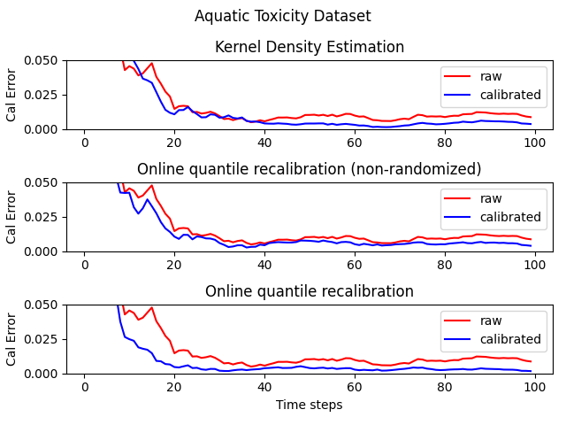
(a) Aquatic Toxicity (Daphnia Magna)

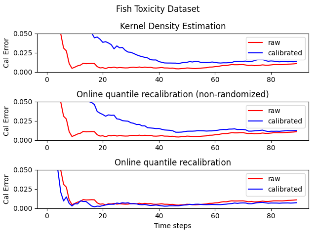
(b) Aquatic Toxicity (Fathead Minnow)

Figure 1: Performance of Online Calibration on the Aquatic Toxicity Datasets. Aquatic toxicity towards two different types of fish (Daphnia Magna 1(a) and Fathead Minnow 1(b)) is predicted by the base model. In both datasets, online calibration outperforms the baseline methods.

$\text{cal}(P_{1},y_{1},..,P_{n},y_{n})=\sum_{j=1}^{m}((p_{j}-p_{j-1})-\hat{p_{j}})^{2},$ where $p_{0}=0<p_{1}<p_{2}<..<p_{m}=1$ are $m$ confidence levels using which we compute the calibration score. $\hat{p_{j}}$ is estimated as $\hat{p_{j}}=|\{y_{t}|p_{j-1}\leq P_{t}\leq p_{j},t=1,..,N\}|/N.$ The calibration scores are computed on each batch of data $\{P_{t},y_{t}\}_{t=nt^{\prime}+1}^{n(t^{\prime}+1)}$, before being observed , where $n$ is the batch size and $t^{\prime}$ is the time-step.

Aquatic Toxicity Datasets

We evaluate our algorithm on the QSAR (Quantitative Structure-Activity Relationship) Aquatic Toxicity Dataset 1(a) and Fish Toxicity Dataset 1(b), where aquatic toxicity towards two different types of fish is predicted using 8 and 6 molecular descriptors as features respectively. In Figure 1, we can see that the randomized online calibration algorithm performs better than the non-randomized baseline by producing lower calibration errors. We also compare the performance of our algorithm against uniform kernel density estimation by maintaining a running average of probabilities in each incoming batch of data-points. For the Fish Toxicity Dataset, we can see that only online calibration improves calibration errors relative to the baseline model. We report the calibration error at the last time-step for all the methods separately in Table 1.

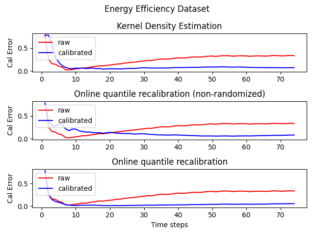
Figure 2: Online recalibration yields low calibration faster than baselines on the Energy dataset.

Energy Efficiency Dataset

In the Energy Efficiency Dataset contains the heating load and cooling load of the building and is predicted using 8 building parameters as features. We set the outcome to the heating load of the building and utilize the 8 features as input to our model. In Figure 2, we see that the calibration errors produced by the online calibration algorithm drop sharply within the initial 10 time-steps. The baselines also produce a drop in calibration scores, but it happens more gradually.

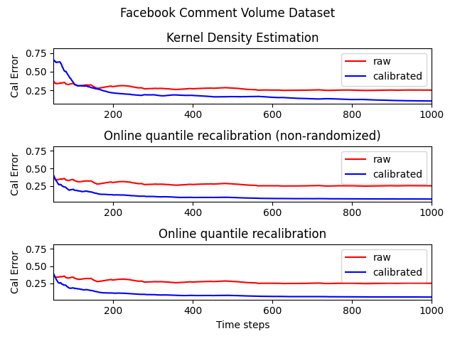
Figure 3: Online recalibration yields the best calibration on Facebook Comments Volume Data

Facebook Comment Volume Dataset

In Figure 3, the Facebook Comment Volume Dataset is used where the number of comments is to be predicted using 53 attributes associated with a post. We use the initial 10000 data-points from the dataset for this experiment. Here, the non-randomized and randomized online calibration algorithms produce a similar drop in calibration errors, but the randomized online calibration algorithm still dominates both the baselines as shown in Table 1.

6.2 Bayesian Optimization

We also apply online recalibration in the context of Bayesian optimization, an online model-based decision-making task in which the data distribution shifts over time. We find that improved uncertainties yield faster convergence to higher quality optima.

Table 2: Recalibrated Bayesian Optimization

Benchmark	Uncalibrated	Recalibrated
Ackley (2D)	9.925 (3.502)	8.313 (3.403)
SixHump (2D)	-0.378 (0.146)	-1.029 (0.002)
Ackley (2D)	14.638 (0.591)	10.867 (2.343)
Alpine (10D)	13.911 (1.846)	12.163 (1.555)

Setup

Bayesian optimization attempts to find the global minimum $x^{\star}=\arg\min_{x\in\mathcal{X}}f(x)$ of an unknown function $f:\mathcal{X}\to\mathbb{R}$ over an input space $\mathcal{X}\subseteq\mathbb{R}^{D}$. We are given an initial labeled dataset $x_{t},y_{t}\in\mathcal{X}\times\mathbb{R}$ for $n=3$. At every time-step $t$, we use normal and recalibrated uncertainties from the probabilistic model $\mathcal{M}:\mathcal{X}\to(\mathbb{R}\to[0,1])$ of $f$ (here, a Gaussian Process) to select the next data-point $x_{next}$ and iteratively update the model $\mathcal{M}$. We use some popular benchmark functions to evaluate the performance of Bayesian optimization. We use the Lower Confidence Bound (LCB) acquisition function to select the data-point $x_{t}$ and evaluate a potentially expensive function $f$ as $x_{t}$ to obtain $y_{t}$. See Appendix C for details.

Table 2 shows that the online recalibration of uncertainties in a Bayesian optimization model achieves lower minima than an uncalibrated model. Figure 4 shows that online recalibrated Bayesian optimization can also reach optima in fewer steps. We also show improvements over calibration without randomization.

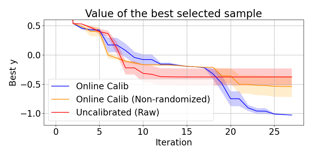
(a) SixHumpCamel

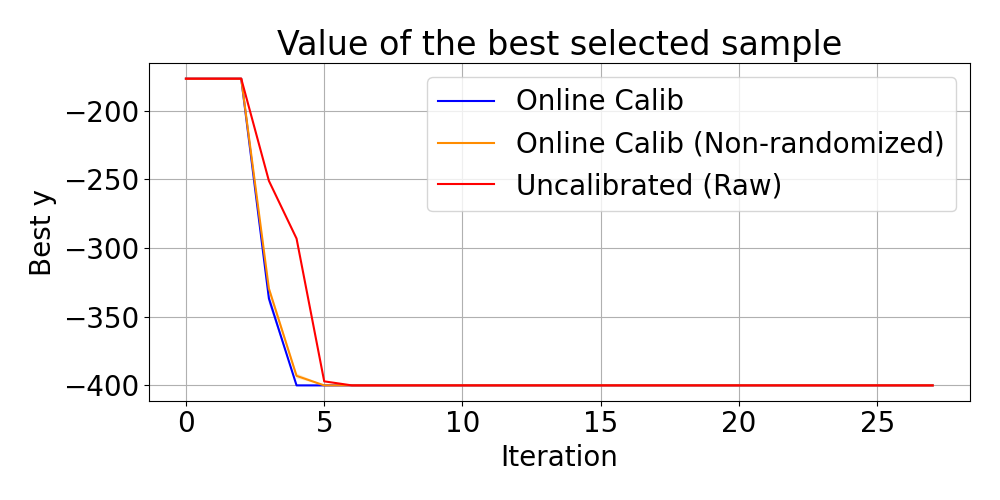
(b) Beale

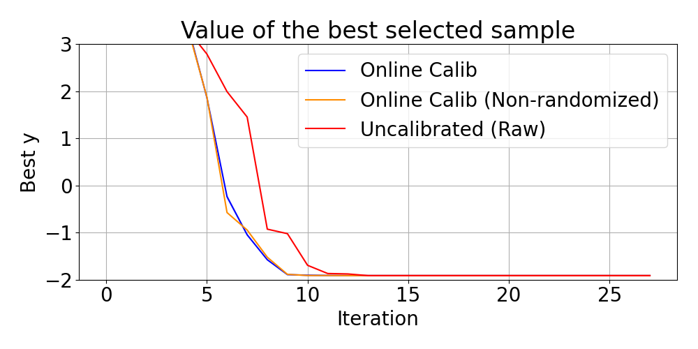
(c) Mccormick

Figure 4: Online Calibration Improves Bayesian optimization

7 Previous Work

Calibrated probabilities are widely used as confidence measures in the context of binary classification. Such probabilities are obtained via recalibration methods, of which Platt scaling [28] and isotonic regression [27] are by far the most popular. Recalibration methods also possess multiclass extensions, which typically involve training multiple one-vs-all predictors [33], as well as extensions to ranking losses [25], combinations of estimators [34], and structured prediction [19]. Recalibration algorithms have applied to improve reinforcement learning [23], Bayesian optimization [9, 30] and deep learning [20].

In the online setting, the calibration problem was formalized by [8]; online calibration techniques were first proposed by [13]. Existing algorithms are based on internal regret minimization [7] or on Blackwell approachability [12]; recently, these approaches were shown to be closely related [1, 24]. Recent work has shown that online calibration is PPAD-hard [17].

The concepts of calibration and sharpness were first formalized in the statistics literature [26, 16]. These metrics are captured by a class of proper losses and can be used both for evaluating [6, 5] and constructing [19] calibrated forecasts.

8 Discussion and Conclusion

Batch vs Online Calibration

Algorithm 2 can be seen as a direct counterpart to the histogram technique, a simple method for density estimation. With the histogram approach, the $F^{H}_{t}$ is split into N bins, and the average y value is estimated for each bin. Because of the i.i.d. assumption, the output probabilities are calibrated, and the bin width determines the sharpness. Note that by Hoeffding’s inequality, the average for a specific bin converges at a faster rate of $O({1}/{\sqrt{T_{j}}})$[10], as opposed to the $O({1}/{\sqrt{\epsilon T_{j}}})$ rate given by Abernethy et al. [1]; hence online calibration is harder than batch.

Conformal Prediction

Conformal prediction [32] is a technique for constructing calibrated predictive sets. It has been extended to handle distribution shifts [18, 31, 4], as well as to online adversarial data [14]. Calibrated prediction [28, 22] is closely related to conformal prediction, but focuses on predicting distributions rather than sets. Our work resembles adaptive conformal inference [14], but provides a distribution-like object instead of one confidence interval and studies a different notion of calibration. As a result, while their algorithm is deterministic, ours is randomized. Unlike their algorithm, ours provides more general vanishing regret guarantees relative to a baseline model.

Deterministic Forecasting

Simultaneously calibrated and accurate online learning methods were developed by [32] in terms of weak calibration [2]. Since we use strong calibration, weak calibration is implied, but it requires different (e.g. randomized) algorithms. Vovk et al.  ensure a small difference between average predicted $p_{t}$ and true $y_{t}$ at times $t$ when $p_{t}\approx p^{*}$ and $x_{t}\approx x^{*}$, for any $p^{*},x^{*}$, by using a different notion of precision. The relation $\approx$ is can be specified by the user via a kernel.

Conclusion

We presented a novel approach to uncertainty estimation that leverages online learning. Our approach extends existing online learning methods to handle predictive uncertainty while ensuring high accuracy, providing formal guarantees on calibration and regret even on adversarial input. We introduced a new problem called online calibrated forecasting, and proposed algorithms that generalize calibrated regression to non-IID settings. Our methods are effective on several predictive tasks and hold potential to improve performance in decision-making settings.

Appendix A Correctness of the recalibration procedure

In the appendix, we provide the proofs of the theorems from the main part of the paper.

Notation

We use ${\mathbb{I}}_{E}$ denote the indicator function of $E$, $[N]$ and $[N]_{0}$ to (respectively) denote the sets $\{1,2,...,N\}$ and $\{0,1,2,...,N\}$, and $\Delta_{d}$ to denote a $d$-dimensional simplex.

Setup

We place our work in the framework of online learning [29]. At each time step $t=1,2,...$, we are given features $x_{t}\in\mathcal{X}$. We use a forecaster $H:\mathcal{X}\to\mathcal{P}$ to produce a prediction $p_{t}=H(x_{t})$, $p_{t}\in\mathcal{P}$ in the set of distributions $\mathcal{P}$ over a target $y\in\mathcal{Y}$. Nature then reveals the true target $y_{t}\in\mathcal{Y}$ and we incur a loss of $\ell(y_{t},p_{t})$, where $\ell:\mathcal{Y}\times\mathcal{P}\to{\mathbb{R}}^{+}$ is a loss function. The forecaster $H$ updates itself based on $x_{t},y_{t}$, and we proceed to time $t+1$.

Unlike in classical machine learning, we do not assume that the $x_{t},y_{t}$ are i.i.d.: they can be random, deterministic or even chosen by an adversary. Online learning algorithms feature strong performance guarantees in this regime, where performance is usually measured in terms of regret $R_{T}(q)$ relative to a constant prediction $q$, $R_{T}(q)=\sum_{t=1}^{T}\ell(y_{t},p_{t})-\ell(y_{t},q).$ The worst-case regret at time $T$ equals $R_{T}=\max_{q\in\mathcal{P}}R_{T}(q)$.

In this paper, the predictions $p_{t}$ are probability distributions over the outcome $y_{t}$. We focus on regression, where $y_{t}\in\mathbb{R}$ and the prediction $p_{t}$ can be represented by a cumulative distribution function (CDF), denoted $F_{t}:\mathbb{R}\to[0,1]$ and defined as $F_{t}(z)=p_{t}(y\leq z)$.

Learning with Expert Advice

A special case of this framework arises when each $x_{t}$ represents advice from $N$ experts, and $H$ outputs $p_{t}\in\Delta_{N-1}$, a distribution over experts. Nature reveals an outcome $y_{t}$, resulting in an expected loss of $\sum_{i=1}^{N}p_{ti}\ell(y_{t},a_{ti})$, where $\ell(y_{t},a_{ti})$ is the loss under expert $i$’s advice $a_{ti}$. Performance in this setting is measured using two notions of regret.

Definition 3.

The external regret $R^{\mathrm{ext}}_{T}$ and the internal regret $R^{\mathrm{int}}_{T}$ are defined as

$$R^{\mathrm{ext}}_{T}=\sum_{t=1}^{T}{\bar{\ell}}(y_{t},p_{t})-\min_{i\in[N]}\sum_{t=1}^{T}\ell(y_{t},a_{it}) R^{\mathrm{int}}_{T}=\max_{i,j\in[N]}\sum_{t=1}^{T}p_{ti}\left(\ell(y_{t},a_{it})-\ell(y_{t},a_{jt})\right),$$

where ${\bar{\ell}}(y,p)=\sum_{i=1}^{N}p_{i}\ell(y,a_{it})$ is the expected loss.

Calibration for Online Binary Calibration

For now, we focus on the $\ell_{1}$ norm, and we define the calibration error of a forecaster $S^{\mathrm{cal}}$ as

$$C_{T}=\sum_{i=0}^{N}\left|\rho_{T}(i/N)-\frac{i}{N}\right|\left(\frac{1}{T}\sum_{t=1}^{T}{\mathbb{I}}_{\{p_{t}=\frac{i}{N}\}}\right),$$ (2)

where $\rho_{T}(p)=\frac{\sum_{t=1}^{T}y_{t}{\mathbb{I}}_{p_{t}=p}}{\sum_{t=1}^{T}{\mathbb{I}}_{p_{t}=p}}$ denotes the frequency at which event $y=1$ occurred over the times when we predicted $p$.

We further define the calibration error when $S^{\mathrm{cal}}_{j}$ predicts $i/N$ as

$$C^{(j)}_{T,i} =\left|{\rho^{(j)}_{T}}(i/N)-\frac{i}{N}\right|\left(\frac{1}{T_{j}}\sum_{t=1}^{T}{\mathbb{I}}^{(j)}_{t,i}\right)$$

where ${\mathbb{I}}^{(j)}_{t,i}={\mathbb{I}}\{p_{t}=\frac{i}{N}\cap F^{H}_{t}\in[\frac{j-1}{M},\frac{j}{M})\}$ is an indicator for the event that $S^{\mathrm{cal}}_{j}$ is triggered at time $t$ and predicts $i/N$. Similarly, ${\mathbb{I}}_{t,i}={\mathbb{I}}\{p_{t}=i/N\}=\sum_{j=1}^{M}{\mathbb{I}}^{(j)}_{t,i}$ indicates that $i/N$ was predicted at time $t$, and $T_{j}=\sum_{t=1}^{T}\sum_{i=0}^{N}{\mathbb{I}}^{(j)}_{t,i}$ is the number of calls to $S^{\mathrm{cal}}_{j}$. Also,

$${\rho^{(j)}_{T}}(i/N)=\frac{\sum_{t=1}^{T}{\mathbb{I}}^{(j)}_{t,i}y_{t}}{\sum_{t=1}^{T}{\mathbb{I}}^{(j)}_{t,i}}$$

is the empirical success rate for $S^{\mathrm{cal}}_{j}$.

Note that with these definitions, we may write the calibration losses of $S^{\mathrm{cal}}_{j}$ as $C^{(j)}_{T}=\sum_{i=0}^{N}C^{(j)}_{T,i}$.

Calibration for Regression

A sequence of forecasts $F_{t}$ achieves online quantile calibration for all $y\in\mathcal{Y}$ and all $p\in\mathcal{P}$, $\rho_{T}(y,p)\to p,$ a.s. as $T\to\infty$, where

$$\rho_{T}(y,p)=\dfrac{\sum_{t=1}^{T}{\mathbb{I}}_{y_{t}\leq y,F_{t}(y)=p}}{\sum_{t=1}^{T}{\mathbb{I}}_{F_{t}(y)=p}}$$

In other words, out of the times when the predicted probability $F_{t}(y^{\prime})$ for $\{y_{t}\leq y^{\prime}\}$ to be $p$, the event $\{y_{t}\leq y^{\prime}\}$ holds a fraction $p$ of the time.

We also seek to quantify more precisely the calibration of Algorithm 2, specifically compare $\rho(y,p)$ with $p$. We define for this the quantity

$$C_{T,i}(y)=\left|\rho_{T}(y,i/N)-\frac{i}{N}\right|\left(\frac{1}{T}\sum_{t=1}^{T}{\mathbb{I}}_{t,i}\right),$$

and we define the calibration loss of Algorithm 2 at $y$ as $C_{T}(y)=\sum_{i=0}^{N}C_{T,i}(y)$.

Proper Losses

The quality of probabilistic forecasts is evaluated using proper losses $\ell$. Formally, a loss $\ell(y,p)$ is proper if $p\in\arg\min_{q\in\mathcal{P}}{\mathbb{E}}_{y\sim(p)}\ell(y,q)\;\forall p\in\mathcal{P}.$ An important proper loss for CDF predictions F is the continuous ranked probability score, defined as

$$\ell_{\text{CRPS}}(y,F)=\int_{-\infty}^{\infty}(F(z)-\mathbb{I}_{y\leq z})^{2}dz.$$

A.1 Assumptions

We assume that each subroutine $S^{\mathrm{cal}}$ is an instance of a binary calibrated forecasting algorithm (e.g., the methods introduced in Chapter 4 in [7]) that produce predictions in $[0,1]$ that are $(\epsilon,\ell_{2})$-calibrated and that $C^{2}_{T}\leq R_{T}+\epsilon$ uniformly ($R_{T}=o(1)$ as $T\to\infty$; $T$ is the number of calls to instance $S^{\mathrm{cal}}_{j}$). We also assume that for each $t$, the target $y_{t}$ lies in some bounded interval $\mathcal{Y}$ of $\mathbb{R}$ of length at most $B$.

A.2 Online Calibrated Regression

First, we look at algorithms for online calibrated regression (without covariates). Our algorithms leverage classical online binary calibration [13] as a subroutine. Formally, Algorithm 1 partitions $[-\frac{B}{2},\frac{B}{2}]$ into $M$ intervals ${\mathcal{I}}=\{[\frac{-B}{2},\frac{-B}{2}+\frac{B}{M}),...,[\frac{B}{2}-\frac{B}{M},\frac{B}{2}]\}$; each interval is associated with an instance of an online binary recalibration subroutine $S^{\mathrm{cal}}$ [13, 7]. In order to compute $G_{t}(y\leq z)$, we invoke the subroutine $S^{\mathrm{cal}}_{j}$ associated with interval $I_{j}$ containing $z$. After observing $y_{t}$, each $S^{\mathrm{cal}}_{j}$ observes whether $y_{t}$ falls in its interval and updates its state.

Theorem 5.

Let $\mathcal{Y}_{\mathcal{I}}$ be the set of upper bounds of the intervals $\mathcal{I}$ and let $\mathcal{P}_{S}$ be the output space of $S^{\mathrm{cal}}$. Algorithm 1 achieves online calibration and for all $y\in\mathcal{Y}_{\mathcal{I}},p\in\mathcal{P}_{S}$ we have $\rho_{T}(y,p)\to p$ a.s. as $T\to\infty$.

Proof.

The above theorem follows directly from the construction of Algorithm 1: for each $y\in\mathcal{Y}$, we run an online binary calibration algorithm to target the event $y_{t}\leq y$.

Specifically, note that for each $y\in\mathcal{Y}_{\mathcal{I}}$, the empirical frequency $\rho(y,p)$ reduces to the definition of the empirical frequency of a classical binary calibration algorithm targeting probability $p$ and the binary outcome that $y_{t}\leq y$. The output of the algorithm for $F_{t}(y)$ is also a prediction for the binary outcome $y_{t}\leq y$ produced by a classical onlne binary calibration algorithm. Thus, by construction, we have the desired result. ∎

Algorithms $S^{\mathrm{cal}}$ for online binary calibration are randomized. Our procedure needs to be randomized as well and this is a fundamental property of our task.

Theorem 6.

There does not exist a deterministic online calibrated regression algorithm that achieves online calibration.

Proof.

This claim follows because we can encode a standard online binary calibration problem as calibrated regression. Specifically, given a non-randomized online calibrated regression algorithm, we could solve an online binary classification problem. Suppose the adversary chooses a binary $y_{t}\in\{0,1\}\subseteq[0,1]$ that defines one of two classes. Then we can define an instance of calibrated regression with two buckets $[0,0.5)$ and $[0.5,1)$. We use the forecast $F_{t}(0.5)$ as our prediction for $y_{t}=0$ and one minus that as the prediction for 1. Then, the error on the ratio $\rho_{T}(0.5,p)$ yields the definition of calibration in binary classification. If our deterministic online calibration regression algorithm works, then we have $\rho_{T}(0.5,p)\to p$, which means that the empirical ratio for the binary algorithm goes to the predicted frequency $p$ as well. But that would yield a deterministic algorithm for online binary calibration, which we know can’t exist. ∎

A.3 Proving the Calibration of Algorithm 2

First, we will provide a proof of Lemma 3; this proof holds for any norm $\ell_{p}$.

Lemma 4 (Preserving calibration).

If each $S^{\mathrm{cal}}_{j}$ is $(\epsilon,\ell_{p})$-calibrated, then Algorithm 2 is also $(\epsilon,\ell_{p})$-calibrated and the following bound holds uniformly over $T$:

$$C_{T}\leq\sum_{j=1}^{M}\frac{T_{j}}{T}R_{T_{j}}+\epsilon.$$ (3)

Proof.

Let ${\mathbb{I}}^{(j)}_{i}=\sum_{t=1}^{T}{\mathbb{I}}^{(j)}_{t,i}$ and note that $\sum_{t=1}^{T}{\mathbb{I}}_{t,i}=\sum_{j=1}^{M}{\mathbb{I}}^{(j)}_{i}$. We may write

$$C_{T,i}(y) =\frac{\sum_{t=1}^{T}{\mathbb{I}}_{t,i}}{T}\left|\rho_{T}(y,i/N)-\frac{i}{N}\right|^{p}=\frac{\sum_{j=1}^{M}{\mathbb{I}}^{(j)}_{i}}{T}\left|\sum_{j=1}^{M}\frac{\sum_{t=1}^{T}{\mathbb{I}}^{(j)}_{t,i}o_{tj}}{\sum_{j=1}^{M}{\mathbb{I}}^{(j)}_{i}}-\frac{i}{N}\right|^{p}$$

$$=\frac{\sum_{j=1}^{M}{\mathbb{I}}^{(j)}_{i}}{T}\left|\sum_{j=1}^{M}\frac{{\mathbb{I}}^{(j)}_{i}{\rho^{(j)}_{T}}(y,i/N)}{\sum_{j=1}^{M}{\mathbb{I}}^{(j)}_{i}}-\frac{i}{N}\right|^{p}\leq\sum_{j=1}^{M}\frac{{\mathbb{I}}^{(j)}_{i}}{T}\left|{\rho^{(j)}_{T}}(y,i/N)-\frac{i}{N}\right|^{p}=\sum_{j=1}^{M}\frac{T_{j}}{T}C^{(j)}_{T,i},$$

where in the last line we used Jensen’s inequality. Plugging in this bound in the definition of $C_{T}$, we find that

$$C_{T} =\sum_{i=1}^{N}C_{T,i}\leq\sum_{j=1}^{M}\sum_{i=1}^{N}\frac{T_{j}}{T}C^{(j)}_{T,i}\leq\sum_{j=1}^{M}\frac{T_{j}}{T}R_{T_{j}}+\epsilon,$$

Since each $R_{T_{j}}\to 0$, Algorithm 2 will be $\epsilon$-calibrated. ∎

A.4 Recalibrated Forecasts Have Low Regret Under the CRPS Loss

Lemma 5 (Recalibration preserves accuracy).

Consider Algorithm 2 with parameters $M\geq N>1/\epsilon$. Suppose that the $S^{\mathrm{cal}}$ are $(\epsilon,\ell_{2})$-calibrated. Then the recalibrated $G_{t}$ a.s. have vanishing $\ell_{\text{CRPS}}$-regret relative to $F_{t}$:

$$\lim_{T\to\infty}\left(\frac{1}{T}\sum_{t=1}^{T}\ell_{\text{CRPS}}(y_{t},G_{t})-\frac{1}{T}\sum_{t=1}^{T}\ell_{\text{CRPS}}(y_{t},F_{t})\right)<2/N.$$ (4)

Proof.

Our proof will rely on the following fact about any online calibration subroutine $S^{\mathrm{cal}}$. We start by formally establishing this fact.

Fact 1.

Let $S^{\mathrm{cal}}$ be an binary online calibration subroutine with actions $0,1/N,...1$ whose $\ell_{2}$ calibration error $C^{p}_{T}$ is bounded by $R_{T}=o(T)$. Then the predictions $p_{t}$ from $S^{\mathrm{cal}}$ also minimize external regret relative to any single action $i/N$:

$$\sum_{t=1}^{T}(p_{t}-y_{t})^{2}-(\frac{i}{N}-y_{t})^{2}\leq NR_{T}\text{ for all }i$$

We refer the reader to Lemma 4.4 in [7] for a proof.

Next, we prove our main claim. We start with some notation. Let ${\mathcal{I}}=\{[0,\frac{1}{M}),[\frac{1}{M},\frac{2}{M}),...,[\frac{M-1}{M},1]\}$ be a set of intervals that partition $[0,1]$ and let $I_{j}=[\frac{j-1}{M},\frac{j}{M})$ be the $j$-th interval. Also, for each $j$, we use $i_{j}$ denote the index $i\in[N]$ that is closest to $j$ in the sense of $|\frac{i_{j}}{N}-\frac{j}{M}|\leq\frac{1}{N}$. By our assumption that $M\geq N$, this index exists.

We begin our proof by from the definition of the CRPS regret:

$$\frac{1}{T}\sum_{t=1}^{T}\ell_{\text{CRPS}}(y_{t},G_{t})-\frac{1}{T}\sum_{t=1}^{T}\ell_{\text{CRPS}}(y_{t},F_{t})$$

$$\;\;=\frac{1}{T}\sum_{t=1}^{T}\int_{-\infty}^{\infty}(G_{t}(z)-\mathbb{I}_{y_{t}\leq z})^{2}dz-\frac{1}{T}\sum_{t=1}^{T}\int_{-\infty}^{\infty}(F_{t}(z)-\mathbb{I}_{y_{t}\leq z})^{2}dz$$

$$\;\;=\int_{-\infty}^{\infty}\frac{1}{T}\sum_{t=1}^{T}\left[(G_{t}(z)-\mathbb{I}_{y_{t}\leq z})^{2}-(F_{t}(z)-\mathbb{I}_{y_{t}\leq z})^{2}\right]dz$$

$$\;\;=\int_{z\in\mathcal{Y}}\frac{1}{T}\sum_{t=1}^{T}\left[(G_{t}(z)-\mathbb{I}_{y_{t}\leq z})^{2}-(F_{t}(z)-\mathbb{I}_{y_{t}\leq z})^{2}\right]dz$$

$$\;\;=\int_{z\in\mathcal{Y}}\frac{1}{T}\sum_{t=1}^{T}\left[(G_{t}(z)-\mathbb{I}_{F_{t}(y_{t})\leq F_{t}(z)})^{2}-(F_{t}(z)-\mathbb{I}_{F_{t}(y_{t})\leq F_{t}(z)})^{2}\right]dz$$

In the second-to-last line, we have used the fact that the forecasts have finite support, i.e., the $y_{t}$ live within a closed bounded set $\mathcal{Y}$. In the last line, we replaced the event $y_{t}\leq z$ with $F_{t}(y_{t})\leq F_{t}(z)$, which is valid because $F_{t}$ is monotonically increasing.

Let’s now analyze the above integrand for one fixed value of $z$:

$$\frac{1}{T}\sum_{t=1}^{T}\left[(G_{t}(z)-\mathbb{I}_{F_{t}(y_{t})\leq F_{t}(z)})^{2}-(F_{t}(z)-\mathbb{I}_{F_{t}(y_{t})\leq F_{t}(z)})^{2}\right].$$

Since $F_{t}$ outputs a finite number of values in the set $\{0,\frac{1}{M},...,1\}$, let $j/M$ denote the value $F_{t}(z)=j/M$ taken by $F_{t}$ at $z$. Additionally, observe that $\mathbb{I}_{F_{t}(y_{t})\leq\frac{j}{M}}=o_{tj}$, where $o_{tj}$ is the binary target variable given to $S^{\mathrm{cal}}_{j}$ at the end of step $t$. Finally, recall that when $F_{t}(z)=\frac{j}{M}$, we have defined $G_{t}(z)$ to be the output of $S^{\mathrm{cal}}_{j}$ at time $t$, which we denote as $G_{tj}$. This yields the following expression for the above integrand for a fixed $z$:

$$\frac{1}{T}\sum_{t=1}^{T}\left[(G_{tj}-o_{tj})^{2}-(\frac{j}{M}-o_{tj})^{2}\right].$$

Next, recall that $i_{j}$ is the index $i\in[N]$ that is closest to $j$ in the sense of $|\frac{i_{j}}{N}-\frac{j}{M}|\leq\frac{1}{N}$. Recall also that $M\geq N$. Note that this implies

$$\ell_{2}(\frac{j}{M},o_{tj})\geq\ell_{2}(\frac{i_{j}}{M},o_{tj})+\frac{\partial\ell_{2}}{\partial p}(p,o_{tj})(\frac{j}{M}-\frac{i_{j}}{M})\geq\frac{2}{N}.$$

Using this inequality, we obtain the following expression for our earlier integrand:

$$\frac{1}{T}\sum_{t=1}^{T}\left[(G_{tj}-o_{tj})^{2}-(\frac{i_{j}}{N}-o_{tj})^{2}\right]+\frac{2}{N}.$$

Crucially, this expression is precisely the external regret of recalibration subroutine $S^{\mathrm{cal}}_{j}$ relative to the fixed action $\frac{i_{j}}{N}$ and measured in terms of the L2 loss. By Fact 1, we know that this external regret is bounded by $NR_{T}$. Since this bound holds pointwise for any value of $z$, we can plug it into our original integral to obtain a bound on the CRPS regret:

$$\int_{z\in\mathcal{Y}}\frac{1}{T}\sum_{t=1}^{T}\left[(G_{t}(z)-\mathbb{I}_{F_{t}(y_{t})\leq F_{t}(z)})^{2}-(F_{t}(z)-\mathbb{I}_{F_{t}(y_{t})\leq F_{t}(z)})^{2}\right]dz$$

$$\;\;\leq\int_{z\in\mathcal{Y}}\left[NR_{T}+\frac{2}{N}\right]dz$$

$$\;\;\leq NBR_{T}+\frac{2B}{N}$$

In the last line, we used the fact that the integration is over a finite set $\mathcal{Y}$ whose measure is bounded by $B>0$. This establishes the main claim of this proposition. ∎

A.5 Correctness of Algorithm 2

We now prove our main result about the correctness of Algorithm 2.

Theorem 1.

Let $S^{\mathrm{cal}}$ be an $(\ell_{1},\epsilon/3B)$-calibrated online subroutine with resolution $N\geq 3B/\epsilon$. and let $\ell$ be a proper loss satisfying the assumptions of Lemma 2. Then Algorithm 2 with parameters $S^{\mathrm{cal}}$ and $N$ is an $\epsilon$-accurate online recalibration algorithm for the loss $\ell$.

Proof.

It is easy to show that Algorithm 2 is $(\ell_{1},\epsilon/3B)$-calibrated by the same argument as Lemma 1 (see the next section for a formal proof). By Lemma 4, its regret w.r.t. the raw $F^{H}_{t}$ tends to $<3B/N<\epsilon$. Hence, the theorem follows. ∎

A.6 Calibration implies no internal regret

Here, we show that a calibrated forecaster also has small internal regret relative to any bounded proper loss [21].

Lemma 1.

If $\ell$ is a bounded proper loss, then an $(\epsilon,\ell_{1})$-calibrated $S^{\mathrm{cal}}$ a.s. has a small internal regret w.r.t. $\ell$ and satisfies uniformly over time $T$ the bound

$$R^{\mathrm{int}}_{T}=\max_{ij}\sum_{t=1}^{T}{\mathbb{I}}_{p_{t}=i/N}\left(\ell(y_{t},i/N)-\ell(y_{t},j/N)\right)\leq 2B(R_{T}+\epsilon).$$ (5)

Proof.

Let $T$ be fixed for the rest of this proof. Let ${\mathbb{I}}_{ti}={\mathbb{I}}_{p_{t}=i/N}$ be the indicator of $S^{\mathrm{cal}}$ outputting prediction $i/N$ at time $t$, let $T_{i}=\sum_{t=1}^{T}{\mathbb{I}}_{ti}$ denote the number of time $i/N$ was predicted, and let

$$R^{\mathrm{int}}_{T,ij}=\sum_{t=1}^{T}{\mathbb{I}}_{ti}\left(\ell(y_{t},i/N)-\ell(y_{t},j/N)\right)$$

denote the gain (measured using the proper loss $\ell$) from retrospectively switching all the plays of action $i$ to $j$. This value forms the basis of the definition of internal regret (Section 2).

Let $T(i,y)=\sum_{t=1}^{T}{\mathbb{I}}_{ti}{\mathbb{I}}\{y_{t}=y\}$ denote the total number of $i/N$ forecasts at times when $y_{t}=y\in\{0,1\}$. Observe that we have

$$T(i,y) =\sum_{t=1}^{T}{\mathbb{I}}_{ti}{\mathbb{I}}\{y_{t}=y\}=\frac{\sum_{t=1}^{T}{\mathbb{I}}_{ti}{\mathbb{I}}\{y_{t}=y\}}{T_{i}}T_{i}=\frac{\sum_{t=1}^{T}{\mathbb{I}}_{ti}{\mathbb{I}}\{y_{t}=y\}}{\sum_{t=1}^{T}{\mathbb{I}}_{ti}}T_{i}$$

$$=q(i,y)T_{i}+T_{i}\left(\frac{\sum_{t=1}^{T}{\mathbb{I}}_{ti}{\mathbb{I}}\{y_{t}=y\}}{\sum_{t=1}^{T}{\mathbb{I}}_{ti}}-q(i,y)\right)$$

$$=q(i,y)T_{i}+T_{i}\left(\rho_{T}(i/N)-i/N\right),$$

where $q(i,y)=i/N$ if $y=1$ and $1-i/N$ if $y=0$. The last equality follows using some simple algebra after adding and subtracting one inside the parentheses in the second term.

We now use this expression to bound $R^{\mathrm{int}}_{T,ij}$:

$$R^{\mathrm{int}}_{T,ij} =\sum_{t=1}^{T}{\mathbb{I}}_{ti}\left(\ell(y_{t},i/N)-\ell(y_{t},j/N)\right)$$

$$=\sum_{y\in\{0,1\}}T(i,y)\left(\ell(y,i/N)-\ell(y,j/N)\right)$$

$$\leq\sum_{y\in\{0,1\}}q(i,y)T_{i}\left(\ell(y,i/N)-\ell(y,j/N)\right)+\sum_{y\in\{0,1\}}BT_{i}\left|\rho_{T}(i/N)-i/N\right|$$

$$\leq 2BT_{i}\left|\rho_{T}(i/N)-i/N\right|,$$

where in the first inequality, we used $\ell(y,i/N)-\ell(y,j/N)\leq\ell(y,i/N)\leq B$, and in the second inequality we used the fact that $\ell$ is a proper loss.

Since internal regret equals $R^{\mathrm{int}}_{T}=\max_{i,j}R^{\mathrm{int}}_{T,ij}$, we have

$$R^{\mathrm{int}}_{T} \leq\sum_{i=1}^{N}\max_{j}R^{\mathrm{int}}_{T,ij}\leq 2B\sum_{i=0}^{N}T_{i}\left|\rho(i/N)-i/N\right|\leq 2B(R_{T}+\epsilon).$$

∎

Appendix B Impossibility of recalibrating non-proper losses

We conclude the appendix by explaining why non-proper losses cannot be calibrated [21].

Theorem 2.

If $\ell$ is not proper, then there is no recalibration algorithm w.r.t. $\ell$.

Proof.

If $\ell$ is not proper, there exist a $p^{\prime}$ and $q$ such that ${\mathbb{E}}_{y\sim\text{Ber}(p^{\prime})}\ell(y,q)<{\mathbb{E}}_{y\sim\text{Ber}(p^{\prime})}\ell(y,p^{\prime})$.

Consider a sequence $y_{t}$ for which $y_{t}\sim\text{Ber}(p^{\prime})$ for all $t$. Clearly the prediction of a calibrated forecaster $p_{t}$ much converge to $p^{\prime}$ and the average loss will approach $\ell(y,p^{\prime})$. This means that we cannot recalibrate the constant predictor $p_{t}=q$ without making its loss $\ell(y,q)$ higher. We thus have a forecaster that cannot be recalibrated with respect to $\ell$. ∎

Appendix C Experiments on Bayesian optimization

Bayesian optimization attempts to find the global minimum $x^{\star}=\arg\min_{x\in\mathcal{X}}f(x)$ of an unknown function $f:\mathcal{X}\to\mathbb{R}$ over an input space $\mathcal{X}\subseteq\mathbb{R}^{D}$. We are given an initial labeled dataset $x_{t},y_{t}\in\mathcal{X}\times\mathbb{R}$ for $t=1,2,...,N$ of i.i.d. realizations of random variables $X,Y\sim P$. At every time-step $t$, we use uncertainties from the probabilistic model $\mathcal{M}:\mathcal{X}\to(\mathbb{R}\to[0,1])$ of $f$ to select the next data-point $x_{next}$ and iteratively update the model $\mathcal{M}$. Algorithm 3 outlines this procedure. Since the black-box function evaluation can be expensive, the objective of Bayesian optimization in this context is to find the minima (or maxima) of this function while using a small number of function evaluations.

We use online calibration to improve the uncertainties estimated by the model $\mathcal{M}$. Following Deshpande and Kuleshov [9], we use Algorithm 5 to recalibrate the model $\mathcal{M}$. Since the dataset size is small, we use the CREATESPLITS function to generate leave-one-out cross-validation splits of our dataset $\mathcal{D}.$ We train the base model on train-split and use this to obtain probabilistic forecast for data in the test-split. We collect these predictions on all test-splits to form our recalibration dataset and use Algorithm 2 to perform calibration.

Following Deshpande and Kuleshov [9], we perform calibrated Bayesian optimization as detailed in Algorithm 4. Specifically, we recalibrate the base model $\mathcal{M}$ after every step in Bayesian optimization.

We use some popular benchmark functions to evaluate the performance of Bayesian optimization. We initialize the Bayesian optimization with 3 randomly chosen data-points. We use the Lower Confidence Bound (LCB) acquisition function to select the data-point $x_{t}$ and evaluate a potentially expensive function $f$ as $x_{t}$ to obtain $y_{t}$. At any given time-step $T$, we have the dataset $\mathcal{D}_{T}=\{x_{t},y_{t}\}_{t=1}^{T}$ collected iteratively.

In Figure 5, we see that using online calibration of uncertainties from $\mathcal{M}$ allows us to reach a lower minimum or find the same minimum with a smaller number of steps with Bayesian optimization.

(a) SixHumpCamel

(b) Beale

(c) Mccormick

Figure 5: Online Calibration Improves Bayesian optimization

Algorithm 3 Bayesian Optimization

1:Initialize base model $\mathcal{M}$ with data $\mathcal{D}=\{x_{t},y_{t}\}_{t=0}^{M}$.

2:for $n=1,2,...,T$: do

3:   $x_{\textrm{next}}$ = $\arg\max_{x\in\mathcal{X}}(\textrm{Acquisition}(x,\mathcal{R}\circ\mathcal{M}))$.

4:   $y_{\textrm{next}}$ = $f(x_{\textrm{next}})$.

5:   $\mathcal{D}$ = $\mathcal{D}\bigcup\{(x_{\textrm{next}},y_{\textrm{next}})\}$

6:   Update model $\mathcal{M}$ with data $\mathcal{D}$

Algorithm 4 Calibrated Bayesian Optimization [9]

1:Initialize base model $\mathcal{M}$ with data $\mathcal{D}=\{x_{t},y_{t}\}_{t=0}^{M}$.

2:$\mathcal{R}\leftarrow\textsc{Calibrate}(\mathcal{M,\mathcal{D}})$.

3:for $n=1,2,...,T$: do

4:   $x_{\textrm{next}}$ = $\arg\max_{x\in\mathcal{X}}(\textrm{Acquisition}(x,\mathcal{R}\circ\mathcal{M}))$.

5:   $y_{\textrm{next}}$ = $f(x_{\textrm{next}})$.

6:   $\mathcal{D}$ = $\mathcal{D}\bigcup\{(x_{\textrm{next}},y_{\textrm{next}})\}$

7:   Update model $\mathcal{M}$ with data $\mathcal{D}$

8:   $\mathcal{R}\leftarrow\textsc{Calibrate}(\mathcal{M,\mathcal{D}})$

Algorithm 5 Calibrate [9]

1:Base model $\mathcal{M}$, Dataset $\mathcal{D}=\{x_{t},y_{t}\}_{t=0}^{N}$

2:Train a base model $\mathcal{M}$ on training dataset $\{x_{t},y_{t}\}_{t=0}^{N}$.

3:Initialize recalibration dataset $\mathcal{D_{\textrm{recal}}}=\phi$

4:$S=\textsc{CreateSplits({D})}$

5:for $(\mathcal{D_{\textrm{train}}},\mathcal{D_{\textrm{test}}})$ in $S$: do

6:   $\mathcal{D_{\textrm{train}}}=$ Train Dataset $\{x_{t},y_{t}\}_{t=0}^{M}$ in split $s$.

7:   $\mathcal{D_{\textrm{test}}}=$ Test Dataset $\{x_{t},y_{t}\}_{t=0}^{L}$ in split $s$.

8:   $\mathcal{D_{\textrm{train}}}=\textsc{TrainSplit}(s),\mathcal{D_{\textrm{test}}}=\textsc{TestSplit}(s)$

9:   Train base model $\mathcal{M^{\prime}}$ on dataset $\mathcal{D_{\textrm{train}}}$

10:   Compute CDF dataset $\{[M^{\prime}(x_{t})](y_{t})\}_{t=1}^{M}$ from dataset $\mathcal{D_{\textrm{test}}}$

11:   $\mathcal{D_{\textrm{recal}}}=\mathcal{D_{\textrm{recal}}}\bigcup\{[\mathcal{M^{\prime}}(x_{t})](y_{t}),y_{t}\}_{t=1}^{M}$

12:Train recalibrator model $\mathcal{R}$ on the recalibration dataset $\mathcal{D_{\textrm{recal}}}$ using Algorithm 2

13:Return ($\mathcal{R}$)

References

- Abernethy et al. [2011] Jacob Abernethy, Peter L. Bartlett, and Elad Hazan. Blackwell approachability and no-regret learning are equivalent. In COLT 2011 - The 24th Annual Conference on Learning Theory, pages 27–46, 2011.
- Abernethy and Mannor [2011] Jacob D. Abernethy and Shie Mannor. Does an efficient calibrated forecasting strategy exist? In COLT 2011 - The 24th Annual Conference on Learning Theory, June 9-11, 2011, Budapest, Hungary, pages 809–812, 2011. URL http://www.jmlr.org/proceedings/papers/v19/abernethy11a/abernethy11a.pdf.
- Angelopoulos and Bates [2021] Anastasios N. Angelopoulos and Stephen Bates. A gentle introduction to conformal prediction and distribution-free uncertainty quantification, 2021. URL https://arxiv.org/abs/2107.07511.
- Barber et al. [2022] Rina Barber, Emmanuel Candes, Aaditya Ramdas, and Ryan Tibshirani. Conformal prediction beyond exchangeability, 02 2022.
- Brocker [2009] J. Brocker. Reliability, sufficiency, and the decomposition of proper scores. Quarterly Journal of the Royal Meteorological Society, 135(643):1512–1519, 2009.
- Buja et al. [2005] Andreas Buja, Werner Stuetzle, and Yi Shen. Loss functions for binary class probability estimation and classification: Structure and applications, 2005.
- Cesa-Bianchi and Lugosi [2006] Nicolo Cesa-Bianchi and Gabor Lugosi. Prediction, Learning, and Games. Cambridge University Press, New York, NY, USA, 2006. ISBN 0521841089.
- Dawid [1982] A. Philip Dawid. The well-calibrated bayesian. Journal of the American Statistical Association, 77(379):605–610, 1982.
- Deshpande and Kuleshov [2021] Shachi Deshpande and Volodymyr Kuleshov. Calibrated uncertainty estimation improves bayesian optimization, 2021. URL https://arxiv.org/abs/2112.04620.
- Devroye et al. [1996] Luc Devroye, László Györfi, and Gábor Lugosi. A probabilistic theory of pattern recognition. Applications of mathematics. Springer, New York, Berlin, Heidelberg, 1996. ISBN 978-0-387-94618-4.
- Dua and Graff [2017] Dheeru Dua and Casey Graff. UCI machine learning repository, 2017. URL http://archive.ics.uci.edu/ml.
- Foster [1997] Dean P. Foster. A Proof of Calibration Via Blackwell’s Approachability Theorem. Discussion Papers 1182, Northwestern University, February 1997.
- Foster and Vohra [1998] Dean P. Foster and Rakesh V. Vohra. Asymptotic calibration, 1998.
- Gibbs and Candès [2021] Isaac Gibbs and Emmanuel Candès. Adaptive conformal inference under distribution shift, 2021. Accepted.
- Gneiting et al. [2007a] Tilmann Gneiting, Fadoua Balabdaoui, and Adrian Raftery. Probabilistic forecasts, calibration and sharpness. Journal of the Royal Statistical Society: Series B (Statistical Methodology), 69:243 – 268, 04 2007a. doi: 10.1111/j.1467-9868.2007.00587.x.
- Gneiting et al. [2007b] Tilmann Gneiting, Fadoua Balabdaoui, and Adrian E. Raftery. Probabilistic forecasts, calibration and sharpness. Journal of the Royal Statistical Society: Series B, 69(2):243–268, 2007b.
- Hazan and Kakade [2012] Elad Hazan and Sham M. Kakade. (weak) calibration is computationally hard. In COLT 2012 - The 25th Annual Conference on Learning Theory, June 25-27, 2012, Edinburgh, Scotland, pages 3.1–3.10, 2012.
- Hendrycks et al. [2018] Dan Hendrycks, Mantas Mazeika, Duncan Wilson, and Kevin Gimpel. Using trusted data to train deep networks on labels corrupted by severe noise, 2018. URL https://arxiv.org/abs/1802.05300.
- Kuleshov and Liang [2015] V. Kuleshov and P. Liang. Calibrated structured prediction. In Advances in Neural Information Processing Systems (NIPS), 2015.
- Kuleshov and Deshpande [2021] Volodymyr Kuleshov and Shachi Deshpande. Calibrated and sharp uncertainties in deep learning via density estimation, 2021. URL https://arxiv.org/abs/2112.07184.
- Kuleshov and Ermon [2017] Volodymyr Kuleshov and Stefano Ermon. Estimating uncertainty online against an adversary. In AAAI, pages 2110–2116, 2017.
- Kuleshov et al. [2018] Volodymyr Kuleshov, Nathan Fenner, and Stefano Ermon. Accurate uncertainties for deep learning using calibrated regression, 2018.
- Malik et al. [2019] Ali Malik, Volodymyr Kuleshov, Jiaming Song, Danny Nemer, Harlan Seymour, and Stefano Ermon. Calibrated model-based deep reinforcement learning. 2019. doi: 10.48550/ARXIV.1906.08312. URL https://arxiv.org/abs/1906.08312.
- Mannor and Stoltz [2010] Shie Mannor and Gilles Stoltz. A geometric proof of calibration. Math. Oper. Res., 35(4):721–727, 2010.
- Menon et al. [2012] Aditya Krishna Menon, Xiaoqian Jiang, Shankar Vembu, Charles Elkan, and Lucila Ohno-Machado. Predicting accurate probabilities with a ranking loss. In 29th International Conference on Machine Learning,, 2012.
- Murphy [1973] A. H. Murphy. A new vector partition of the probability score. Journal of Applied Meteorology, 12(4):595–600, 1973.
- Niculescu-Mizil and Caruana [2005] Alexandru Niculescu-Mizil and Rich Caruana. Predicting good probabilities with supervised learning. In Proceedings of the 22Nd International Conference on Machine Learning, ICML ’05, 2005.
- Platt [1999] John C. Platt. Probabilistic outputs for support vector machines and comparisons to regularized likelihood methods. In ADVANCES IN LARGE MARGIN CLASSIFIERS, pages 61–74. MIT Press, 1999.
- Shalev-Shwartz [2007] Shai Shalev-Shwartz. Online Learning: Theory, Algorithms, and Applications. Phd thesis, Hebrew University, 2007.
- Stanton et al. [2023] Samuel Stanton, Wesley Maddox, and Andrew Gordon Wilson. Bayesian optimization with conformal prediction sets, 2023.
- Tibshirani et al. [2019] Ryan J. Tibshirani, Rina Foygel Barber, Emmanuel J. Candes, and Aaditya Ramdas. Conformal prediction under covariate shift, 2019. URL https://arxiv.org/abs/1904.06019.
- Vovk et al. [2005] Vladimir Vovk, Akimichi Takemura, and Glenn Shafer. Defensive forecasting. In Proceedings of the Tenth International Workshop on Artificial Intelligence and Statistics, AISTATS 2005, Bridgetown, Barbados, January 6-8, 2005, 2005. URL http://www.gatsby.ucl.ac.uk/aistats/fullpapers/224.pdf.
- Zadrozny and Elkan [2002] Bianca Zadrozny and Charles Elkan. Transforming classifier scores into accurate multiclass probability estimates. In Eighth ACM Conference on Knowledge Discovery and Data Mining, pages 694–699, 2002.
- Zhong and Kwok [2013] Leon Wenliang Zhong and James T. Kwok. Accurate probability calibration for multiple classifiers. IJCAI ’13, pages 1939–1945. AAAI Press, 2013. ISBN 978-1-57735-633-2.