Abstract

The explorations of models beyond the Standard Model (BSM) naturally involve scans over the unknown BSM parameters. On the other hand, high precision predictions require calculations at the loop-level and thus a renormalization of (some of) the BSM parameters. Often many choices are possible for the renormalization scheme (RS). This concerns the choice of the set of to-be-renormalized parameters out of a larger set of BSM parameters, but can also concern the type of renormalization condition which is chosen for a specific parameter. A given RS can be well suited to yield “stable” and “well behaved” higher-order corrections in one part of the BSM parameter space, but can fail completely in other parts, which may not even be noticed numerically if an isolated parameter point is investigated, or when the higher-order BSM calculations are performed in an automated, not supervised set-up. Consequently, the (automated) exploration of BSM models requires a choice of a good RS before the calculation is performed. We propose a new method how such a choice can be performed. We demonstrate the feasibility of our new method in the chargino/neutralino sector of the Minimal Supersymmetric Standard Model (MSSM), but stress the general applicability of our method to all types of BSM models.

1 Introduction

The Standard Model (SM) provides a good description of nearly all experimental data in high-energy physics. On the other hand, there is clear evidence that the SM cannot be the ultimate theory. Gravity is not included, it does not contain a suitable Dark Matter candidate, it does not explain the Baryon asymmetry in the universe, neutrinos are massles, etc. Consequently,the explorations of models beyond the Standard Model (BSM) is one of the main tasks of the upcoming LHC Runs, including the high-luminosity LHC (HL-LHC), as well as possible future collider projects. Reliable investigations, going beyond the very initial exploration of a BSM model requires the inclusion of higher-order corrections to, e.g., the production cross sections of BSM particles at the HL-LHC. This in turn requires the renormalization of the BSM model.

The renormalization of BSM models is much less explored than the renormalization of the SM [2, 3]. Examples for “full one-loop renormalizations” can be found for the Two Higgs Doublet Model (2HDM) [4, 5, 6] (see also Ref. [7]), the Minimal Supersymmetric Standard Model (MSSM) [8, 9, 10, 11], and the Next-to-MSSM (NMSSM) [12, 13, 14, 15, 16]. These analyses showed that many different choices of renormalization schemes (RS) are possible. This can concern the choice of the set of to-be-renormalized parameters out of a larger set of BSM parameters, but can also concern the type of renormalization condition that is chosen for a specific parameter.

BSM models naturally possess several new BSM parameters. The number of new parameters can vary from ${\cal O}(1)$ to ${\cal O}(10)$, or even higher. Often multi-dimensional parameter scans are employed, or methods such as Markow-Chain Monte-Carlo (MCMC) analyses [17, 18] to find the phenomenological best-appealing parameters in the multi-dimensional BSM parameter space. The above mentioned BSM analyses also demonstrated that a given RS can be well suited to yield “stable” and “well behaved” higher-order corrections (more details will be given below) in one part of the BSM parameter space, but can fail completely in other parts. The latter may not even be noticed numerically if only isolated parameter points are investigated, which is natural in a scan, or MCMC analyses. Consequently, the exploration of BSM models requires a choice of a good RS before the calculation is performed.

An RS “fails” if one of the counterterms (or a linear combination of counterterms) does not (or only marginally) depend on the parameter itself, but is rather determined via other parameters of the model. This failure can manifest itself in

• “unnaturally” large higher-order corrections,

• large (numerical) differences between $\smash{\overline{\mathrm{DR}}}$ and OS masses,

• large (numerical) differences between $\smash{\overline{\mathrm{DR}}}$ and OS parameters.

In this work we propose a new method how such a situation can be avoided, i.e. how a “good” RS can be chosen. This method is based on the properties of the transformation matrix that connects the various counter terms with the underlying parameters. This allows a point-by-point test of all “available” or “possible” RS, and the “best” one can be chosen to perform the calculation. Only this type of selection of a good RS before the calculation will allow a fully automated set-up of BSM higher-order calculations.

Our idea is designed to work in all cases of RS choices (in BSM models). In the detailed definition we will, however, tackle a slightly more specific question: in many BSM models one can be faced with the situation that one has $m$ underlying Lagrangian parameters and $n>m$ particles or particle masses that can be renormalized on-shell (OS). The calculation of the production and/or decay of BSM particles naturally requires OS renormalizations of the particles involved. Each choice of $m$ particles renormalized OS defines an $\mbox{RS}_{l}$, of which we have $N$ in total. We will demonstrate how out of these $N$ $\mbox{RS}_{l}$ one can choose the “best” $\mbox{RS}_{L}$.

The numerical examples will be performed within the MSSM, concretely in the sector of charginos and neutralinos, the supersymmetric (SUSY) partners of the SM gauge bosons and the 2HDM-like Higgs sector. While this constitutes a very specific example, we would like to stress the general applicability of our method to all types of BSM models and types of RS choices.

The paper is organized as follows. In Sect. 2 we present our general idea how to choose $n$ particles to be renormalized OS, when only $m<n$ free parameters are available. The concrete implementation for the chargino/neutralino sector will be given in Sect. 3. Here we will define this sector in all details, discuss which different schemes are available and explain the treatment of the $m-n$ particles that cannot be renormalized OS. In Sect. 4 we present concrete numerical examples and demonstrate that our method selects a stable and well behaved renormalization over the full parameter space. Our conclusions are given in Sect. 5.

2 General idea

As discussed above, the idea of how to choose a stable and well behaved RS is generally applicable. However, here we will outline it focusing a more concrete problem: in our theory we have $m$ underlying Lagrangian parameters and $n>m$ particles or particle masses that can be renormalized OS. Each choice of $m$ particles renormalized OS defines an $\mbox{RS}_{l}$, of which we have $N$ in total. How can one choose the “best” $\mbox{RS}_{L}$?

There are two possible starting points for input parameters in our analysis:

• The masses of the BSM particles under investigation have not (yet) been measured. Then we start with $\smash{\overline{\mathrm{DR}}}$ parameters.

• All the masses (or a subset) have been determined experimentally. Then one starts with OS masses (or a subset of them).

Currently, we are clearly in the $\smash{\overline{\mathrm{DR}}}$ case. Consequently, we will focus on the $\smash{\overline{\mathrm{DR}}}$ choice, and leave the OS case for future work.

The general idea for the automated choice of the $\mbox{RS}_{L}$ in the $\smash{\overline{\mathrm{DR}}}$ case can be outlined for two possible levels of refinement. The first one is called “semi-OS scheme”, and the second one “full-OS scheme” (where in our numerical examples we will focus on the latter). The two cases are defined as follows.

Semi-OS scheme:

1. We start with $m$ $\smash{\overline{\mathrm{DR}}}$ parameters, $P_{i}^{\smash{\overline{\mathrm{DR}}}}$, from the Lagrangian.

2. We have $N$ $\mbox{RS}_{l}$.

3. For each $\mbox{RS}_{l}$, i.e. each different choice of $m$ particles renormalized OS, we evaluate the corresponding OS parameters

   $$P_{i,l}^{\mathrm{os}}=P_{i}^{\smash{\overline{\mathrm{DR}}}}-\delta P_{i,l|{\rm fin}}^{\mathrm{os}}$$ (1)

   with the transformation matrix $\mathbf{A}^{\smash{\overline{\mathrm{DR}}}}_{l}$ (more details will be given below).

4. It will be argued that a “bad” scheme $\mbox{RS}_{l}$ has a small or even vanishing $|\det\mathbf{A}^{\smash{\overline{\mathrm{DR}}}}_{l}|$.

5. Comparing the various $|\det\mathbf{A}^{\smash{\overline{\mathrm{DR}}}}_{l}|$ yields $\mbox{RS}_{L}$.

6. Inserting $P_{i,L}^{\mathrm{os}}$ into the Lagrangian yields $n$ particle masses out of which $m$ are by definition given as their OS values. The remaining OS masses have to be determined calculating $n-m$ finite shifts.

7. The counterterms for the $P_{i,L}^{\mathrm{os}}$ are already known from Eq. (1) as $\delta P_{i,L}^{\mathrm{os}}$ and can be inserted as counterterms in a loop calculation.

This procedure yields all ingredients for an OS scheme. However, the OS counterterms $\delta P_{i,L}^{\mathrm{os}}$ and thus also the OS parameters themselves, $P_{i,L}^{\mathrm{os}}$, are calculated in terms of $\smash{\overline{\mathrm{DR}}}$ parameters, i.e. one has $\delta P_{i,L}^{\mathrm{os}}(P_{i}^{\smash{\overline{\mathrm{DR}}}})$ and $P_{i,L}^{\mathrm{os}}(P_{i}^{\smash{\overline{\mathrm{DR}}}})$. This is unsatisfactory for a “true” OS scheme, i.e. one would like to have $\delta P_{i,L}^{\mathrm{OS}}(P_{i,L}^{\mathrm{OS}})$. Furthermore, when a $\mbox{RS}_{l}$ “starts to turn bad” as a function of a $\smash{\overline{\mathrm{DR}}}$ parameter, large differences between the $P_{i,l}^{\mathrm{os}}$ and $P_{i}^{\smash{\overline{\mathrm{DR}}}}$ occur, shedding doubt on the above outlined procedure. These problems can be circumvented by extending the above scheme to an evaluation of the counterterms in terms of OS parameters. The general idea starts as above, but deviates from step 4 on.

Full-OS scheme:

1. We start with $m$ $\smash{\overline{\mathrm{DR}}}$ parameters, $P_{i}^{\smash{\overline{\mathrm{DR}}}}$, from the Lagrangian.

2. We have $N$ $\mbox{RS}_{l}$.

3. For each $\mbox{RS}_{l}$, i.e. each different choice of $m$ particles renormalized OS, we evaluate the corresponding OS parameters

   $$P_{i,l}^{\mathrm{os}}=P_{i}^{\smash{\overline{\mathrm{DR}}}}-\delta P_{i,l|{\rm fin}}^{\mathrm{os}}$$ (2)

   with the transformation matrix $\mathbf{A}^{\smash{\overline{\mathrm{DR}}}}_{l}$ (more details will be given below).

4. Inserting $P_{i,l}^{\mathrm{os}}$ into the Lagrangian yields $n$ particle masses out of which $m$ are by definition given as their $\mathrm{os}_{l}$ values. The remaining $\mathrm{os}_{l}$ masses have to be determined calculating $n-m$ finite shifts.

5. $\mbox{RS}_{l}$ is applied again on the OS_l Lagrangian.

6. This yields now OS counterterms in terms of $\mathrm{os}_{l}$ parameters,

   $$\delta P_{i,l}^{\mathrm{OS}}(P_{i,l}^{\mathrm{os}})$$ (3)

   with the transformation matrix $\mathbf{A}_{l}^{\mathrm{OS}}$ (more details will be given below).

7. It will be argued that a “bad” scheme $\mbox{RS}_{l}$ has a small or even vanishing $|\det\mathbf{A}^{\smash{\overline{\mathrm{DR}}}}_{l}|$ and/or $|\det\mathbf{A}^{\mathrm{OS}}_{l}|$.

8. Comparing the various

   $$\min\left\{|\det\mathbf{A}^{\smash{\overline{\mathrm{DR}}}}_{l}|,|\det\mathbf{A}^{\mathrm{OS}}_{l}|\right\}$$ (4)

   yields $\mbox{RS}_{L}$.

9. The counterterms for the $P_{i,L}^{\mathrm{OS}}$ are already known from Eq. (3) as $\delta P_{i,L}^{\mathrm{OS}}$ and can be inserted as counterterms in a loop calculation.

Steps 4-6 could be iterated until convergence is reached. We will not do this.

In the following sections we will explain and demonstrate the concrete implementation of this procedure for the case of the chargino/neutralino sector in the MSSM.

3 Concrete implementation

The concrete implementation concerns the calculation of physics processes with (external) charginos and/or neutralinos, $\tilde{\chi}_{c}^{\pm}(c=1,2)$ and $\tilde{\chi}_{n}^{0}(n=1,2,3,4)$ at the loop level. This requires the choice of a (numerically well behaved) RS. The possible scheme choices are ($n^{\prime\prime}>n^{\prime}>n$)

$$\mbox{CCN}_{n},\quad\mbox{CNN}_{cnn^{\prime}},\quad\mbox{NNN}_{nn^{\prime}n^{\prime\prime}}\quad c=1,2;\;n,n^{\prime},n^{\prime\prime}=1,2,3,4~{}.$$ (5)

Here $\mbox{CCN}_{n}$ denotes a scheme where the two charginos and the neutralino $n$, $\tilde{\chi}_{n}^{0}$, are renormalized OS. $\mbox{CNN}_{cnn^{\prime}}$ denotes a scheme were chargino $c$, $\tilde{\chi}_{c}^{\pm}$, as well as neutralinos $n,n^{\prime}$, $\tilde{\chi}_{n}^{0},\tilde{\chi}_{n^{\prime}}^{0}$, are renormalized OS. Finally $\mbox{NNN}_{nn^{\prime}n^{\prime\prime}}$ denotes a scheme with three neutralinos renormalized OS (see also Ref. [19]). For sake of simplicity, in the following we neglect the $\mbox{NNN}_{nn^{\prime}n^{\prime\prime}}$ schemes.

In the following we will describe the concrete implementation of the general scheme described in Sect. 2 in the case of the chargino/neutralino sector of the MSSM. The starting point will be $\smash{\overline{\mathrm{DR}}}$ input parameters. The case of an observation of (parts of) the spectrum is beyond the scope of this publication.

3.1 Notation

In this section we briefly review our notation of the chargino/neutralino sector of the MSSM, as well as the relevant (derived) quantities, such as (renormalized) self-energies and mass shifts (more details and applications can be found in Refs. [20, 21, 22, 23, 24]).

The starting point for the renormalization of the chargino/neutralino sector is the part of the Fourier transformed MSSM Lagrangian which is bilinear in the chargino and neutralino fields,

$${\cal L}^{\text{bil.}}_{\tilde{\chi}^{-},\tilde{\chi}^{0}} =\overline{\tilde{\chi}_{i}^{-}}\,\makebox[0.86108pt][l]{$p$}/\,\omega_{-}\tilde{\chi}_{i}^{-}+\overline{\tilde{\chi}_{i}^{-}}\,\makebox[0.86108pt][l]{$p$}/\,\omega_{+}\tilde{\chi}_{i}^{-}-\overline{\tilde{\chi}_{i}^{-}}\,[\mathbf{V}^{*}\mathbf{X}^{\top}\mathbf{U}^{\dagger}]_{ij}\,\omega_{-}\tilde{\chi}_{j}^{-}-\overline{\tilde{\chi}_{i}^{-}}\,[\mathbf{U}\mathbf{X}^{*}\mathbf{V}^{\top}]_{ij}\,\omega_{+}\tilde{\chi}_{j}^{-}$$

$$\quad+\frac{1}{2}\left(\overline{\tilde{\chi}_{k}^{0}}\,\makebox[0.86108pt][l]{$p$}/\,\omega_{-}\tilde{\chi}_{k}^{0},+\overline{\tilde{\chi}_{k}^{0}}\,\makebox[0.86108pt][l]{$p$}/\,\omega_{+}\tilde{\chi}_{k}^{0}-\overline{\tilde{\chi}_{k}^{0}}\,[\mathbf{N}^{*}\mathbf{Y}\mathbf{N}^{\dagger}]_{kl}\,\omega_{-}\tilde{\chi}_{l}^{0}-\overline{\tilde{\chi}_{k}^{0}}\,[\mathbf{N}\mathbf{Y}^{*}\mathbf{N}^{\top}]_{kl}\,\omega_{+}\tilde{\chi}_{l}^{0}\right)~{},$$ (6)

already expressed in terms of the chargino and neutralino mass eigenstates $\tilde{\chi}_{i}^{-}$ and $\tilde{\chi}_{k}^{0}$, respectively, and $i,j=1,2$ and $k,l=1,2,3,4$. The mass eigenstates can be determined via unitary transformations where the corresponding matrices diagonalize the chargino and neutralino mass matrix, $\mathbf{X}$ and $\mathbf{Y}$, respectively.

In the chargino case, two $2\times 2$ matrices $\mathbf{U}$ and $\mathbf{V}$ are necessary for the diagonalization of the chargino mass matrix $\mathbf{X}$,

$$\mathbf{M}_{\tilde{\chi}^{-}}=\mathbf{V}^{*}\,\mathbf{X}^{\top}\,\mathbf{U}^{\dagger}=\begin{pmatrix}m_{\tilde{\chi}^{\pm}_{1}}&0\\ 0&m_{\tilde{\chi}^{\pm}_{2}}\end{pmatrix}\quad\text{with}\quad\mathbf{X}=\begin{pmatrix}M_{2}&\sqrt{2}\sin\beta\,M_{W}\\ \sqrt{2}\cos\beta\,M_{W}&\mu\end{pmatrix}~{},$$ (7)

where $\mathbf{M}_{\tilde{\chi}^{-}}$ is the diagonal mass matrix with the chargino masses $m_{\tilde{\chi}_{1}^{\pm}},m_{\tilde{\chi}_{2}^{\pm}}$ as entries, which are determined as the (real and positive) singular values of $\mathbf{X}$. The singular value decomposition of $\mathbf{X}$ also yields results for $\mathbf{U}$ and $\mathbf{V}$. Using the transformation matrices $\mathbf{U}$ and $\mathbf{V}$, the interaction Higgsino and wino spinors $\tilde{H}^{-}_{1}$, $\tilde{H}^{+}_{2}$ and $\tilde{W}^{\pm}$, which are two component Weyl spinors, can be transformed into the mass eigenstates

$$\tilde{\chi}_{i}^{-}=\begin{pmatrix}\psi^{L}_{i}\\ \overline{\psi^{R}_{i}}\end{pmatrix}\quad\text{with}\quad\psi^{L}_{i}=U_{ij}\begin{pmatrix}\tilde{W}^{-}\\ \tilde{H}^{-}_{1}\end{pmatrix}_{j}\quad\text{and}\quad\psi^{R}_{i}=V_{ij}\begin{pmatrix}\tilde{W}^{+}\\ \tilde{H}^{+}_{2}\end{pmatrix}_{j}$$ (8)

where the $i$th mass eigenstate can be expressed in terms of either the Weyl spinors $\psi^{L}_{i}$ and $\psi^{R}_{i}$ or the Dirac spinor $\tilde{\chi}_{i}^{-}$.

In the neutralino case, as the neutralino mass matrix $\mathbf{Y}$ is symmetric, one $4\times 4$ matrix is sufficient for the diagonalization

$$\mathbf{M}_{\tilde{\chi}^{0}}=\mathbf{N}^{*}\,\mathbf{Y}\,\mathbf{N}^{\dagger}=\text{\bf diag}(m_{\tilde{\chi}_{1}^{0}},m_{\tilde{\chi}_{2}^{0}},m_{\tilde{\chi}_{3}^{0}},m_{\tilde{\chi}_{4}^{0}})$$ (9)

with

$$\mathbf{Y} =\begin{pmatrix}M_{1}&0&-M_{Z}\,s_{\mathrm{w}}\cos\beta\,&M_{Z}\,s_{\mathrm{w}}\sin\beta\,\\ 0&M_{2}&\quad M_{Z}\,c_{\mathrm{w}}\cos\beta\,&-M_{Z}\,c_{\mathrm{w}}\sin\beta\,\\ -M_{Z}\,s_{\mathrm{w}}\cos\beta\,&M_{Z}\,c_{\mathrm{w}}\cos\beta\,&0&-\mu\\ \quad M_{Z}\,s_{\mathrm{w}}\sin\beta\,&-M_{Z}\,c_{\mathrm{w}}\sin\beta\,&-\mu&0\end{pmatrix}~{}.$$ (10)

$M_{Z}$ and $M_{W}$ are the masses of the $Z$ and $W$ boson, $c_{\mathrm{w}}=M_{W}/M_{Z}$ and $s_{\mathrm{w}}=\sqrt{1-c_{\mathrm{w}}^{2}}$. The unitary 4$\times$4 matrix $\mathbf{N}$ and the physical neutralino (tree-level) masses $m_{\tilde{\chi}_{k}^{0}}$ ($k=1,2,3,4$) result from a numerical Takagi factorization [25] of $\mathbf{Y}$. Starting from the original bino/wino/higgsino basis, the mass eigenstates can be determined with the help of the transformation matrix $\mathbf{N}$,

$$\tilde{\chi}_{k}^{0}=\begin{pmatrix}\psi^{0}_{k}\\[1.99997pt] \overline{\psi^{0}_{k}}\end{pmatrix}\qquad\text{with}\qquad\psi^{0}_{k}=N_{kl}{\left(\tilde{B}^{0},\tilde{W}^{0},\tilde{H}^{0}_{1},\tilde{H}^{0}_{2}\right)^{\top}_{l}}$$ (11)

where $\psi^{0}_{k}$ denotes the two component Weyl spinor and $\tilde{\chi}_{k}^{0}$ the four component Majorana spinor of the $k$th neutralino field.

Concerning the renormalization of this sector, the following replacements of the parameters and the fields are performed according to the multiplicative renormalization procedure, which is formally identical for the two set-ups:

$$M_{1}\; \to\;M_{1}+\delta M_{1}~{},$$ (12)

$$M_{2}\; \to\;M_{2}+\delta M_{2}~{},$$ (13)

$$\mu\; \to\;\mu+\delta\mu~{},$$ (14)

$$\omega_{-}\tilde{\chi}_{i}^{\pm}\; \to\;\left[{\rm 1\kern-1.19995pt\rule{0.3pt}{6.45831pt}\raisebox{0.0pt}{\rule{1.00006pt}{0.3pt}}}+\tfrac{1}{2}\delta\mathbf{Z}_{\tilde{\chi}^{\pm}}^{L}\right]_{ij}\omega_{-}\tilde{\chi}_{j}^{\pm}\qquad(i,j=1,2)~{},$$ (15)

$$\omega_{+}\tilde{\chi}_{i}^{\pm}\; \to\;\left[{\rm 1\kern-1.19995pt\rule{0.3pt}{6.45831pt}\raisebox{0.0pt}{\rule{1.00006pt}{0.3pt}}}+\tfrac{1}{2}\delta\mathbf{Z}_{\tilde{\chi}^{\pm}}^{R}\right]_{ij}\omega_{+}\tilde{\chi}_{j}^{\pm}\qquad(i,j=1,2)~{},$$ (16)

$$\omega_{-}\tilde{\chi}_{k}^{0}\; \to\;\left[{\rm 1\kern-1.19995pt\rule{0.3pt}{6.45831pt}\raisebox{0.0pt}{\rule{1.00006pt}{0.3pt}}}+\tfrac{1}{2}\delta\mathbf{Z}_{\tilde{\chi}^{0}}\right]_{kl}\omega_{-}\tilde{\chi}_{l}^{0}\qquad(k,l=1,2,3,4)~{},$$ (17)

$$\omega_{+}\tilde{\chi}_{k}^{0}\; \to\;\left[{\rm 1\kern-1.19995pt\rule{0.3pt}{6.45831pt}\raisebox{0.0pt}{\rule{1.00006pt}{0.3pt}}}+\tfrac{1}{2}\delta\mathbf{Z}_{\tilde{\chi}^{0}}^{*}\right]_{kl}\omega_{+}\tilde{\chi}_{l}^{0}\qquad(k,l=1,2,3,4)~{}.$$ (18)

It should be noted that the parameter counterterms are complex counterterms which each need two renormalization conditions to be fixed. The transformation matrices are not renormalized, so that, using the notation of replacing a matrix by its renormalized matrix and a counterterm matrix

$$\mathbf{X} \to\mathbf{X}+\delta\mathbf{X}~{},$$ (19)

$$\mathbf{Y} \to\mathbf{Y}+\delta\mathbf{Y}~{}$$ (20)

with

$$\delta\mathbf{X} =\begin{pmatrix}\delta M_{2}&\sqrt{2}\,\delta(M_{W}\sin\beta)\\ \sqrt{2}\,\delta(M_{W}\cos\beta)&\delta\mu\end{pmatrix}~{},$$ (21)

$$\delta\mathbf{Y} =\begin{pmatrix}\delta M_{1}&0&-\delta(M_{Z}s_{\mathrm{w}}\cos\beta)&\delta(M_{Z}s_{\mathrm{w}}\sin\beta)\\ 0&\delta M_{2}&\delta(M_{Z}c_{\mathrm{w}}\cos\beta)&-\delta(M_{Z}c_{\mathrm{w}}\sin\beta)\\ -\delta(M_{Z}s_{\mathrm{w}}\cos\beta)&\delta(M_{Z}c_{\mathrm{w}}\cos\beta)&0&-\delta\mu\\ \delta(M_{Z}s_{\mathrm{w}}\sin\beta)&-\delta(M_{Z}c_{\mathrm{w}}\sin\beta)&-\delta\mu&0\end{pmatrix}~{},$$ (22)

the replacements of the matrices $\mathbf{M}_{\tilde{\chi}^{-}}$ and $\mathbf{M}_{\tilde{\chi}^{0}}$ can be expressed as

$$\mathbf{M}_{\tilde{\chi}^{-}} \to\mathbf{M}_{\tilde{\chi}^{-}}+\delta\mathbf{M}_{\tilde{\chi}^{-}}=\mathbf{M}_{\tilde{\chi}^{-}}+\mathbf{V}^{*}\delta\mathbf{X}^{\top}\mathbf{U}^{\dagger}$$ (23)

$$\mathbf{M}_{\tilde{\chi}^{0}} \to\mathbf{M}_{\tilde{\chi}^{0}}+\delta\mathbf{M}_{\tilde{\chi}^{0}}=\mathbf{M}_{\tilde{\chi}^{0}}+\mathbf{N}^{*}\delta\mathbf{Y}\mathbf{N}^{\dagger}~{}.$$ (24)

For convenience, we decompose the self-energies into left- and right-handed vector and scalar coefficients via

$$\left[\Sigma_{\tilde{\chi}}(p^{2})\right]_{nm}=\displaystyle{\not}p\,{\omega_{-}}\left[\Sigma_{\tilde{\chi}}^{L}(p^{2})\right]_{nm}+\displaystyle{\not}p\,{\omega_{+}}\left[\Sigma_{\tilde{\chi}}^{R}(p^{2})\right]_{nm}+{\omega_{-}}\left[\Sigma_{\tilde{\chi}}^{SL}(p^{2})\right]_{nm}+{\omega_{+}}\left[\Sigma_{\tilde{\chi}}^{SR}(p^{2})\right]_{nm}~{}.$$ (25)

Now the coefficients of the renormalized self-energies are given by $(i,j=1,2;k,l=1,2,3,4)$

$$\left[\hat{\Sigma}_{\tilde{\chi}^{\pm}}^{L}(p^{2})\right]_{ij} =\left[\Sigma_{\tilde{\chi}^{\pm}}^{L}(p^{2})\right]_{ij}+\tfrac{1}{2}\left[\delta\mathbf{Z}_{\tilde{\chi}^{\pm}}^{L}+\delta\mathbf{Z}_{\tilde{\chi}^{\pm}}^{L\dagger}\right]_{ij}~{},$$ (26)

$$\left[\hat{\Sigma}_{\tilde{\chi}^{\pm}}^{R}(p^{2})\right]_{ij} =\left[\Sigma_{\tilde{\chi}^{\pm}}^{R}(p^{2})\right]_{ij}+\tfrac{1}{2}\left[\delta\mathbf{Z}_{\tilde{\chi}^{\pm}}^{R}+\delta\mathbf{Z}_{\tilde{\chi}^{\pm}}^{R\dagger}\right]_{ij}~{},$$ (27)

$$\left[\hat{\Sigma}_{\tilde{\chi}^{\pm}}^{SL}(p^{2})\right]_{ij} =\left[\Sigma_{\tilde{\chi}^{\pm}}^{SL}(p^{2})\right]_{ij}-\left[\tfrac{1}{2}\delta\mathbf{Z}_{\tilde{\chi}^{\pm}}^{R\dagger}\mathbf{M}_{\tilde{\chi}^{-}}+\tfrac{1}{2}\mathbf{M}_{\tilde{\chi}^{-}}\delta\mathbf{Z}_{\tilde{\chi}^{\pm}}^{L}+\delta\mathbf{M}_{\tilde{\chi}^{-}}\right]_{ij}~{},$$ (28)

$$\left[\hat{\Sigma}_{\tilde{\chi}^{\pm}}^{SR}(p^{2})\right]_{ij} =\left[\Sigma_{\tilde{\chi}^{\pm}}^{SR}(p^{2})\right]_{ij}-\left[\tfrac{1}{2}\delta\mathbf{Z}_{\tilde{\chi}^{\pm}}^{L\dagger}\mathbf{M}_{\tilde{\chi}^{-}}^{\dagger}+\tfrac{1}{2}\mathbf{M}_{\tilde{\chi}^{-}}^{\dagger}\delta\mathbf{Z}_{\tilde{\chi}^{\pm}}^{R}+\delta\mathbf{M}_{\tilde{\chi}^{-}}^{\dagger}\right]_{ij}~{},$$ (29)

$$\left[\hat{\Sigma}_{\tilde{\chi}^{0}}^{L}(p^{2})\right]_{kl} =\left[\Sigma_{\tilde{\chi}^{0}}^{L}(p^{2})\right]_{kl}+\tfrac{1}{2}\left[\delta\mathbf{Z}_{\tilde{\chi}^{0}}+\delta\mathbf{Z}_{\tilde{\chi}^{0}}^{\dagger}\right]_{kl}~{},$$ (30)

$$\left[\hat{\Sigma}_{\tilde{\chi}^{0}}^{R}(p^{2})\right]_{kl} =\left[\Sigma_{\tilde{\chi}^{0}}^{R}(p^{2})\right]_{kl}+\tfrac{1}{2}\left[\delta\mathbf{Z}_{\tilde{\chi}^{0}}^{*}+\delta\mathbf{Z}_{\tilde{\chi}^{0}}^{\top}\right]_{kl}~{},$$ (31)

$$\left[\hat{\Sigma}_{\tilde{\chi}^{0}}^{SL}(p^{2})\right]_{kl} =\left[\Sigma_{\tilde{\chi}^{0}}^{SL}(p^{2})\right]_{kl}-\left[\tfrac{1}{2}\delta\mathbf{Z}_{\tilde{\chi}^{0}}^{\top}\mathbf{M}_{\tilde{\chi}^{0}}+\tfrac{1}{2}\mathbf{M}_{\tilde{\chi}^{0}}\delta\mathbf{Z}_{\tilde{\chi}^{0}}+\delta\mathbf{M}_{\tilde{\chi}^{0}}\right]_{kl}~{},$$ (32)

$$\left[\hat{\Sigma}_{\tilde{\chi}^{0}}^{SR}(p^{2})\right]_{kl} =\left[\Sigma_{\tilde{\chi}^{0}}^{SR}(p^{2})\right]_{kl}-\left[\tfrac{1}{2}\delta\mathbf{Z}_{\tilde{\chi}^{0}}^{\dagger}\mathbf{M}_{\tilde{\chi}^{0}}^{\dagger}+\tfrac{1}{2}\mathbf{M}_{\tilde{\chi}^{0}}^{\dagger}\delta\mathbf{Z}_{\tilde{\chi}^{0}}^{*}+\delta\mathbf{M}_{\tilde{\chi}^{0}}^{\dagger}\right]_{kl}~{}.$$ (33)

In the following we will give some general expressions for a chargino or neutralino to be renormalized OS. The OS conditions read:

$$\Bigl{(}\left[\widetilde{\mathop{\mathrm{Re}}}\hat{\Sigma}_{\tilde{\chi}^{-}}(p)\right]_{ii}\tilde{\chi}_{i}^{-}(p)\Bigr{)}\Big{|}_{p^{2}=m_{\tilde{\chi}_{i}^{\pm}}^{2}} =0\qquad(i=1,2)~{},$$ (34)

$$\quad\Bigl{(}\left[\widetilde{\mathop{\mathrm{Re}}}\hat{\Sigma}_{\tilde{\chi}^{0}}(p)\right]_{kk}\tilde{\chi}_{k}^{0}(p)\Bigr{)}\Big{|}_{p^{2}=m_{\tilde{\chi}_{k}^{0}}^{2}} =0\qquad(k=1,2,3,4)~{}.$$ (35)

These conditions can be rewritten in terms of the expressions for the renormalized self-energies,

$$\widetilde{\mathop{\mathrm{Re}}}\left[m_{\tilde{\chi}_{i}^{\pm}}\left(\hat{\Sigma}_{\tilde{\chi}^{-}}^{L}(m_{\tilde{\chi}_{i}^{\pm}}^{2})+\hat{\Sigma}_{\tilde{\chi}^{-}}^{R}(m_{\tilde{\chi}_{i}^{\pm}}^{2})\right)+\hat{\Sigma}_{\tilde{\chi}^{-}}^{SL}(m_{\tilde{\chi}_{i}^{\pm}}^{2})+\hat{\Sigma}_{\tilde{\chi}^{-}}^{SR}(m_{\tilde{\chi}_{i}^{\pm}}^{2})\right]_{ii} =0~{},$$ (36)

$$\widetilde{\mathop{\mathrm{Re}}}\left[m_{\tilde{\chi}_{i}^{\pm}}\left(\hat{\Sigma}_{\tilde{\chi}^{-}}^{L}(m_{\tilde{\chi}_{i}^{\pm}}^{2})-\hat{\Sigma}_{\tilde{\chi}^{-}}^{R}(m_{\tilde{\chi}_{i}^{\pm}}^{2})\right)-\hat{\Sigma}_{\tilde{\chi}^{-}}^{SL}(m_{\tilde{\chi}_{i}^{\pm}}^{2})+\hat{\Sigma}_{\tilde{\chi}^{-}}^{SR}(m_{\tilde{\chi}_{i}^{\pm}}^{2})\right]_{ii} =0~{},$$ (37)

$$\widetilde{\mathop{\mathrm{Re}}}\left[m_{\tilde{\chi}_{k}^{0}}\left(\hat{\Sigma}_{\tilde{\chi}^{0}}^{L}(m_{\tilde{\chi}_{k}^{0}}^{2})+\hat{\Sigma}_{\tilde{\chi}^{0}}^{R}(m_{\tilde{\chi}_{k}^{0}}^{2})\right)+\hat{\Sigma}_{\tilde{\chi}^{0}}^{SL}(m_{\tilde{\chi}_{k}^{0}}^{2})+\hat{\Sigma}_{\tilde{\chi}^{0}}^{SR}(m_{\tilde{\chi}_{k}^{0}}^{2})\right]_{kk} =0~{},$$ (38)

$$\widetilde{\mathop{\mathrm{Re}}}\left[m_{\tilde{\chi}_{k}^{0}}\left(\hat{\Sigma}_{\tilde{\chi}^{0}}^{L}(m_{\tilde{\chi}_{k}^{0}}^{2})-\hat{\Sigma}_{\tilde{\chi}^{0}}^{R}(m_{\tilde{\chi}_{k}^{0}}^{2})\right)-\hat{\Sigma}_{\tilde{\chi}^{0}}^{SL}(m_{\tilde{\chi}_{k}^{0}}^{2})+\hat{\Sigma}_{\tilde{\chi}^{0}}^{SR}(m_{\tilde{\chi}_{k}^{0}}^{2})\right]_{kk} =0~{}.$$ (39)

Equations (37) and (39) are related to the axial and axial-vector component of the renormalized self energy and therefore the l.h.s. vanishes in the case of real couplings. Therefore, in the rMSSM only Eqs. (36) and (38) remain. It should be noted that since the lightest neutralino is stable there are no absorptive contributions from its self energy and $\widetilde{\mathop{\mathrm{Re}}}$ can be dropped from Eqs. (35,38,39) for $k=1$.

For the further determination of the field renormalization constants, we also impose

$$\lim_{p^{2}\to m_{\tilde{\chi}_{i}^{\pm}}^{2}}\Bigl{(}\frac{(\makebox[0.86108pt][l]{$p$}/\,+m_{\tilde{\chi}_{i}^{\pm}})\bigl{[}\widetilde{\mathop{\mathrm{Re}}}\hat{\Sigma}_{\tilde{\chi}^{-}}(p)\bigr{]}_{ii}}{p^{2}-m_{\tilde{\chi}_{i}^{\pm}}^{2}}\tilde{\chi}_{i}^{-}(p)\Bigr{)} =0\qquad(i=1,2)~{},$$ (40)

$$\lim_{p^{2}\to{m_{\tilde{\chi}_{k}^{0}}^{2}}}\Bigl{(}\frac{(\makebox[0.86108pt][l]{$p$}/\,+{m_{\tilde{\chi}_{k}^{0}}})\bigl{[}\widetilde{\mathop{\mathrm{Re}}}\hat{\Sigma}_{\tilde{\chi}^{0}}(p)\bigr{]}_{{kk}}}{p^{2}-{m_{\tilde{\chi}_{k}^{0}}^{2}}}{\tilde{\chi}_{k}^{0}}(p)\Bigr{)} =0\qquad(k=1,2,3,4)~{},$$ (41)

which, together with Eqs. (37) and (39), lead to the following set of equations

$$\widetilde{\mathop{\mathrm{Re}}}\Bigl{[}\tfrac{1}{2}\left(\hat{\Sigma}_{\tilde{\chi}^{-}}^{L}(m_{\tilde{\chi}_{i}^{\pm}}^{2})+\hat{\Sigma}_{\tilde{\chi}^{-}}^{R}(m_{\tilde{\chi}_{i}^{\pm}}^{2})\right)+m_{\tilde{\chi}_{i}^{\pm}}^{2}\left(\hat{\Sigma}_{\tilde{\chi}^{-}}^{L^{\prime}}(m_{\tilde{\chi}_{i}^{\pm}}^{2})+\hat{\Sigma}_{\tilde{\chi}^{-}}^{R^{\prime}}(m_{\tilde{\chi}_{i}^{\pm}}^{2})\right)\quad\$$

$$+m_{\tilde{\chi}_{i}^{\pm}}\left(\hat{\Sigma}_{\tilde{\chi}^{-}}^{SL^{\prime}}(m_{\tilde{\chi}_{i}^{\pm}}^{2})+\hat{\Sigma}_{\tilde{\chi}^{-}}^{SR^{\prime}}(m_{\tilde{\chi}_{i}^{\pm}}^{2})\right)\Bigr{]}_{ii} =0~{},$$ (42)

$$\widetilde{\mathop{\mathrm{Re}}}\left[\hat{\Sigma}_{\tilde{\chi}^{-}}^{L}(m_{\tilde{\chi}_{i}^{\pm}}^{2})-\hat{\Sigma}_{\tilde{\chi}^{-}}^{R}(m_{\tilde{\chi}_{i}^{\pm}}^{2})\right]_{ii} =0~{},$$ (43)

$$\widetilde{\mathop{\mathrm{Re}}}\Bigl{[}\tfrac{1}{2}\left(\hat{\Sigma}_{\tilde{\chi}^{0}}^{L}(m_{\tilde{\chi}_{{k}}^{0}}^{2})+\hat{\Sigma}_{\tilde{\chi}^{0}}^{R}(m_{\tilde{\chi}_{{k}}^{0}}^{2})\right)+m_{\tilde{\chi}_{{k}}^{0}}^{2}\left(\hat{\Sigma}_{\tilde{\chi}^{0}}^{L^{\prime}}(m_{\tilde{\chi}_{{k}}^{0}}^{2})+\hat{\Sigma}_{\tilde{\chi}^{0}}^{R^{\prime}}(m_{\tilde{\chi}_{{k}}^{0}}^{2})\right)\quad\$$

$$+m_{\tilde{\chi}_{{k}}^{0}}\left(\hat{\Sigma}_{\tilde{\chi}^{0}}^{SL^{\prime}}(m_{\tilde{\chi}_{{k}}^{0}}^{2})+\hat{\Sigma}_{\tilde{\chi}^{0}}^{SR^{\prime}}(m_{\tilde{\chi}_{{k}}^{0}}^{2})\right)\Bigr{]}_{{kk}} =0~{},$$ (44)

$$\widetilde{\mathop{\mathrm{Re}}}\left[\hat{\Sigma}_{\tilde{\chi}^{0}}^{L}(m_{\tilde{\chi}_{{k}}^{0}}^{2})-\hat{\Sigma}_{\tilde{\chi}^{0}}^{R}(m_{\tilde{\chi}_{{k}}^{0}}^{2})\right]_{{kk}} =0~{},$$ (45)

where we have used the short-hand $\Sigma^{\prime}(m^{2})\equiv(\partial\Sigma/\partial p^{2})|_{p^{2}=m^{2}}$. It should be noted that Eq. (45) is already fulfilled due to the Majorana nature of the neutralinos.

Inserting Eqs. (26) – (33) for the renormalized self-energies in Eqs. (36) – (39) and solving for $\left[\delta\mathbf{M}_{\tilde{\chi}^{-}}\right]_{ii}$ and $\left[\delta\mathbf{M}_{\tilde{\chi}^{0}}\right]_{11}$ results in

$$\mathop{\mathrm{Re}}\left[\delta\mathbf{M}_{\tilde{\chi}^{-}}\right]_{ii} =\frac{1}{2}\widetilde{\mathop{\mathrm{Re}}}\left[m_{\tilde{\chi}_{i}^{\pm}}\left(\Sigma_{\tilde{\chi}^{\pm}}^{L}(m_{\tilde{\chi}_{i}^{\pm}}^{2})+\Sigma_{\tilde{\chi}^{\pm}}^{R}(m_{\tilde{\chi}_{i}^{\pm}}^{2})\right)+\Sigma_{\tilde{\chi}^{\pm}}^{SL}(m_{\tilde{\chi}_{i}^{\pm}}^{2})+\Sigma_{\tilde{\chi}^{\pm}}^{SR}(m_{\tilde{\chi}_{i}^{\pm}}^{2})\right]_{ii}~{},$$ (46)

$$\mathop{\mathrm{Im}}\left[\delta\mathbf{M}_{\tilde{\chi}^{-}}\right]_{ii} =\frac{i}{2}\widetilde{\mathop{\mathrm{Re}}}\left[\Sigma_{\tilde{\chi}^{\pm}}^{SR}(m_{\tilde{\chi}_{i}^{\pm}}^{2})-\Sigma_{\tilde{\chi}^{\pm}}^{SL}(m_{\tilde{\chi}_{i}^{\pm}}^{2})\right]_{ii}-\frac{1}{2}m_{\tilde{\chi}_{i}^{\pm}}\mathop{\mathrm{Im}}\left[\delta\mathbf{Z}_{\tilde{\chi}^{-}}^{L}-\delta\mathbf{Z}_{\tilde{\chi}^{-}}^{R}\right]_{ii}~{},$$ (47)

$$\mathop{\mathrm{Re}}\left[\delta\mathbf{M}_{\tilde{\chi}^{0}}\right]_{kk} =\frac{1}{2}\widetilde{\mathop{\mathrm{Re}}}\left[m_{\tilde{\chi}_{k}^{0}}\left(\Sigma_{\tilde{\chi}^{0}}^{L}(m_{\tilde{\chi}_{1}^{0}}^{2})+\Sigma_{\tilde{\chi}^{0}}^{R}(m_{\tilde{\chi}_{1}^{0}}^{2})\right)+\Sigma_{\tilde{\chi}^{0}}^{SL}(m_{\tilde{\chi}_{k}^{0}}^{2})+\Sigma_{\tilde{\chi}^{0}}^{SR}(m_{\tilde{\chi}_{k}^{0}}^{2})\right]_{kk}~{},$$ (48)

$$\mathop{\mathrm{Im}}\left[\delta\mathbf{M}_{\tilde{\chi}^{0}}\right]_{kk} =\frac{i}{2}\widetilde{\mathop{\mathrm{Re}}}\left[\Sigma_{\tilde{\chi}^{0}}^{SR}(m_{\tilde{\chi}_{k}^{0}}^{2})-\Sigma_{\tilde{\chi}^{0}}^{SL}(m_{\tilde{\chi}_{k}^{0}}^{2})\right]_{kk}-m_{\tilde{\chi}_{k}^{0}}\mathop{\mathrm{Im}}\bigl{[}\delta\mathbf{Z}_{\tilde{\chi}^{0}}\bigr{]}_{kk}~{},$$ (49)

where we have used the relations (43) and (45).

Eqs. (42) and (44) define the real part of the diagonal field renormalization constants of the chargino fields and of the lightest neutralino field. The imaginary parts of the diagonal field renormalization constants are still undefined. However, they can be obtained using Eqs. (47) and (49). For the charginos and neutralinos Eqs. (47) and (49) define the imaginary parts of $\left[\delta\mathbf{M}_{\tilde{\chi}^{\pm}}\right]_{ii}$ ($i=1,2$), and $\left[\delta\mathbf{M}_{\tilde{\chi}^{0}}\right]_{kk}$ ($k=1,2,3,4$) in terms of the imaginary part of the field renormalization constants. Therefore these are simply set to zero (see below Eqs. (53) and (56)), which is possible as all divergences are absorbed by other counterterms.

The off-diagonal field renormalization constants are fixed by the condition that

$$\Bigl{(}\left[\widetilde{\mathop{\mathrm{Re}}}\hat{\Sigma}_{\tilde{\chi}^{-}}(p)\right]_{ij}\tilde{\chi}_{j}^{-}(p)\Bigr{)}\Big{|}_{p^{2}=m_{\tilde{\chi}_{j}^{\pm}}^{2}} =0\qquad(i,j=1,2)~{},$$ (50)

$$\Bigl{(}\left[\widetilde{\mathop{\mathrm{Re}}}\hat{\Sigma}_{\tilde{\chi}^{0}}(p)\right]_{kl}\tilde{\chi}_{l}^{0}(p)\Bigr{)}\Big{|}_{p^{2}=m_{\tilde{\chi}_{l}^{0}}^{2}} =0\qquad(k,l=1,2,3,4)~{}.$$ (51)

Finally, this yields for the field renormalization constants [26] (where we now make the correct dependence on tree-level and on-shell masses explicit),

$$\mathop{\mathrm{Re}}\left[\delta\mathbf{Z}_{\tilde{\chi}^{\pm}}^{L/R}\right]_{ii} =-\widetilde{\mathop{\mathrm{Re}}}\Big{[}\Sigma_{\tilde{\chi}^{\pm}}^{L/R}(m_{\tilde{\chi}_{i}^{\pm}}^{2})$$ (52)

$$\qquad+m_{\tilde{\chi}_{i}^{\pm}}^{2}\left(\Sigma_{\tilde{\chi}^{\pm}}^{L^{\prime}}(m_{\tilde{\chi}_{i}^{\pm}}^{2})+\Sigma_{\tilde{\chi}^{\pm}}^{R^{\prime}}(m_{\tilde{\chi}_{i}^{\pm}}^{2})\right)+m_{\tilde{\chi}_{i}^{\pm}}\left(\Sigma_{\tilde{\chi}^{\pm}}^{SL^{\prime}}(m_{\tilde{\chi}_{i}^{\pm}}^{2})+\Sigma_{\tilde{\chi}^{\pm}}^{SR^{\prime}}(m_{\tilde{\chi}_{i}^{\pm}}^{2})\right)\Big{]}_{ii}~{},$$

$$\mathop{\mathrm{Im}}\left[\delta\mathbf{Z}_{\tilde{\chi}^{\pm}}^{L/R}\right]_{ii} =\pm\frac{1}{m_{\tilde{\chi}_{i}^{\pm}}}\left[\frac{i}{2}\widetilde{\mathop{\mathrm{Re}}}\left\{\Sigma_{\tilde{\chi}^{\pm}}^{SR}(m_{\tilde{\chi}_{i}^{\pm}}^{2})-\Sigma_{\tilde{\chi}^{\pm}}^{SL}(m_{\tilde{\chi}_{i}^{\pm}}^{2})\right\}-\mathop{\mathrm{Im}}\delta\mathbf{M}_{\tilde{\chi}^{-}}\right]_{ii}\stackrel{{\scriptstyle\mathrm{S_{I}}}}{{:=}}0~{},$$ (53)

$$\left[\delta\mathbf{Z}_{\tilde{\chi}^{\pm}}^{L/R}\right]_{ij} =\frac{2}{m_{\tilde{\chi}_{i}^{\pm}}^{2}-m_{\tilde{\chi}_{j}^{\pm}}^{2}}\widetilde{\mathop{\mathrm{Re}}}\Big{[}m_{\tilde{\chi}_{j}^{\pm}}^{2}\Sigma_{\tilde{\chi}^{\pm}}^{L/R}(m_{\tilde{\chi}_{j}^{\pm}}^{2})+m_{\tilde{\chi}_{i}^{\pm}}m_{\tilde{\chi}_{j}^{\pm}}\Sigma_{\tilde{\chi}^{\pm}}^{R/L}(m_{\tilde{\chi}_{j}^{\pm}}^{2})$$ (54)

$$\qquad+m_{\tilde{\chi}_{i}^{\pm}}\Sigma_{\tilde{\chi}^{\pm}}^{SL/SR}(m_{\tilde{\chi}_{j}^{\pm}}^{2})+m_{\tilde{\chi}_{j}^{\pm}}\Sigma_{\tilde{\chi}^{\pm}}^{SR/SL}(m_{\tilde{\chi}_{j}^{\pm}}^{2})-m_{\tilde{\chi}_{i/j}^{\pm}}\delta\mathbf{M}_{\tilde{\chi}^{-}}-m_{\tilde{\chi}_{j/i}^{\pm}}\delta\mathbf{M}_{\tilde{\chi}^{-}}^{\dagger}\Big{]}_{ij}~{},$$

$$\mathop{\mathrm{Re}}\left[\delta\mathbf{Z}_{\tilde{\chi}^{0}}\right]_{kk} =-\widetilde{\mathop{\mathrm{Re}}}\Big{[}\Sigma_{\tilde{\chi}^{0}}^{L}(\hat{m}_{\tilde{\chi}^{0}_{k}}^{2})$$ (55)

$$\qquad+m_{\tilde{\chi}_{k}^{0}}^{2}\left(\Sigma_{\tilde{\chi}^{0}}^{L^{\prime}}(\hat{m}_{\tilde{\chi}^{0}_{k}}^{2})+\Sigma_{\tilde{\chi}^{0}}^{R^{\prime}}(\hat{m}_{\tilde{\chi}^{0}_{k}}^{2})\right)+m_{\tilde{\chi}_{k}^{0}}\left(\Sigma_{\tilde{\chi}^{0}}^{SL^{\prime}}(\hat{m}_{\tilde{\chi}^{0}_{k}}^{2})+\Sigma_{\tilde{\chi}^{0}}^{SR^{\prime}}(\hat{m}_{\tilde{\chi}^{0}_{k}}^{2})\right)\Big{]}_{kk}~{},$$

$$\mathop{\mathrm{Im}}\left[\delta\mathbf{Z}_{\tilde{\chi}^{0}}\right]_{kk} =\frac{1}{m_{\tilde{\chi}_{k}^{0}}}\left[\frac{i}{2}\widetilde{\mathop{\mathrm{Re}}}\left\{\Sigma_{\tilde{\chi}^{0}}^{SR}(\hat{m}_{\tilde{\chi}^{0}_{k}}^{2})-\Sigma_{\tilde{\chi}^{0}}^{SL}(\hat{m}_{\tilde{\chi}^{0}_{k}}^{2})\right\}-\mathop{\mathrm{Im}}\delta\mathbf{M}_{\tilde{\chi}^{0}}\right]_{kk}\stackrel{{\scriptstyle k=1,\,\,\mathrm{S_{I}}}}{{:=}}0~{},$$ (56)

$$\left[\delta\mathbf{Z}_{\tilde{\chi}^{0}}\right]_{kl} =\frac{2}{m_{\tilde{\chi}_{k}^{0}}^{2}-m_{\tilde{\chi}_{l}^{0}}^{2}}\widetilde{\mathop{\mathrm{Re}}}\Big{[}m_{\tilde{\chi}_{l}^{0}}^{2}\Sigma_{\tilde{\chi}^{0}}^{L}(\hat{m}_{\tilde{\chi}^{0}_{l}}^{2})+m_{\tilde{\chi}_{k}^{0}}m_{\tilde{\chi}_{l}^{0}}\Sigma_{\tilde{\chi}^{0}}^{R}(\hat{m}_{\tilde{\chi}^{0}_{l}}^{2})$$

$$\qquad+m_{\tilde{\chi}_{k}^{0}}\Sigma_{\tilde{\chi}^{0}}^{SL}(\hat{m}_{\tilde{\chi}^{0}_{l}}^{2})+m_{\tilde{\chi}_{l}^{0}}\Sigma_{\tilde{\chi}^{0}}^{SR}(\hat{m}_{\tilde{\chi}^{0}_{l}}^{2})-m_{\tilde{\chi}_{k}^{0}}\delta\mathbf{M}_{\tilde{\chi}^{0}}-m_{\tilde{\chi}_{l}^{0}}\delta\mathbf{M}_{\tilde{\chi}^{0}}^{\dagger}\Big{]}_{kl}~{}.$$ (57)

Contributions to the partial decay widths can arise from the product of the imaginary parts of the loop-functions (absorptive contributions) of the self-energy type contributions in the external legs and the imaginary parts of complex couplings entering the decay vertex or the self-energies. It is possible to combine these additional contributions with the field renormalization constants in a single “$Z$ factor”, $\mathcal{Z}$, see e.g. Ref. [11, 20] and references therein. In our notation they read (unbarred for an incoming neutralino or a negative chargino, barred for an outgoing neutralino or negative chargino),

$$\left[\delta{\cal Z}_{\tilde{\chi}^{\pm}}^{L/R}\right]_{ii} =-\Big{[}\Sigma_{\tilde{\chi}^{\pm}}^{L/R}(m_{\tilde{\chi}_{i}^{\pm}}^{2})$$ (58)

$$\qquad+m_{\tilde{\chi}_{i}^{\pm}}^{2}\left(\Sigma_{\tilde{\chi}^{\pm}}^{L^{\prime}}(m_{\tilde{\chi}_{i}^{\pm}}^{2})+\Sigma_{\tilde{\chi}^{\pm}}^{R^{\prime}}(m_{\tilde{\chi}_{i}^{\pm}}^{2})\right)+m_{\tilde{\chi}_{i}^{\pm}}\left(\Sigma_{\tilde{\chi}^{\pm}}^{SL^{\prime}}(m_{\tilde{\chi}_{i}^{\pm}}^{2})+\Sigma_{\tilde{\chi}^{\pm}}^{SR^{\prime}}(m_{\tilde{\chi}_{i}^{\pm}}^{2})\right)\Big{]}_{ii}~{}$$

$$\qquad\pm\frac{1}{2m_{\tilde{\chi}_{i}^{\pm}}}\left[\Sigma_{\tilde{\chi}^{\pm}}^{SL}(m_{\tilde{\chi}_{i}^{\pm}}^{2})-\Sigma_{\tilde{\chi}^{\pm}}^{SR}(m_{\tilde{\chi}_{i}^{\pm}}^{2})-\delta\mathbf{M}_{\tilde{\chi}^{-}}+\delta\mathbf{M}_{\tilde{\chi}^{-}}^{*}\right]_{ii}~{},$$

$$\left[\delta{\cal Z}_{\tilde{\chi}^{\pm}}^{L/R}\right]_{ij} =\frac{2}{m_{\tilde{\chi}_{i}^{\pm}}^{2}-m_{\tilde{\chi}_{j}^{\pm}}^{2}}\Big{[}m_{\tilde{\chi}_{j}^{\pm}}^{2}\Sigma_{\tilde{\chi}^{\pm}}^{L/R}(m_{\tilde{\chi}_{j}^{\pm}}^{2})+m_{\tilde{\chi}_{i}^{\pm}}m_{\tilde{\chi}_{j}^{\pm}}\Sigma_{\tilde{\chi}^{\pm}}^{R/L}(m_{\tilde{\chi}_{j}^{\pm}}^{2})$$ (59)

$$\qquad+m_{\tilde{\chi}_{i}^{\pm}}\Sigma_{\tilde{\chi}^{\pm}}^{SL/SR}(m_{\tilde{\chi}_{j}^{\pm}}^{2})+m_{\tilde{\chi}_{j}^{\pm}}\Sigma_{\tilde{\chi}^{\pm}}^{SR/SL}(m_{\tilde{\chi}_{j}^{\pm}}^{2})-m_{\tilde{\chi}_{i/j}^{\pm}}\delta\mathbf{M}_{\tilde{\chi}^{-}}-m_{\tilde{\chi}_{j/i}^{\pm}}\delta\mathbf{M}_{\tilde{\chi}^{-}}^{\dagger}\Big{]}_{ij}~{},$$

$$\left[\delta{\cal Z}_{\tilde{\chi}^{0}}^{L/R}\right]_{kk} =-\Big{[}\Sigma_{\tilde{\chi}^{0}}^{L/R}(\hat{m}_{\tilde{\chi}^{0}_{k}}^{2})$$ (60)

$$\qquad+m_{\tilde{\chi}_{k}^{0}}^{2}\left(\Sigma_{\tilde{\chi}^{0}}^{L^{\prime}}(\hat{m}_{\tilde{\chi}^{0}_{k}}^{2})+\Sigma_{\tilde{\chi}^{0}}^{R^{\prime}}(\hat{m}_{\tilde{\chi}^{0}_{k}}^{2})\right)+m_{\tilde{\chi}_{k}^{0}}\left(\Sigma_{\tilde{\chi}^{0}}^{SL^{\prime}}(\hat{m}_{\tilde{\chi}^{0}_{k}}^{2})+\Sigma_{\tilde{\chi}^{0}}^{SR^{\prime}}(\hat{m}_{\tilde{\chi}^{0}_{k}}^{2})\right)\Big{]}_{kk}$$

$$\qquad\pm\frac{1}{2m_{\tilde{\chi}_{k}^{0}}}\left[\Sigma_{\tilde{\chi}^{0}}^{SL}(\hat{m}_{\tilde{\chi}^{0}_{k}}^{2})-\Sigma_{\tilde{\chi}^{0}}^{SR}(\hat{m}_{\tilde{\chi}^{0}_{k}}^{2})-\delta\mathbf{M}_{\tilde{\chi}^{0}}+\delta\mathbf{M}_{\tilde{\chi}^{0}}^{*}\right]_{kk}~{},$$

$$\left[\delta{\cal Z}_{\tilde{\chi}^{0}}^{L/R}\right]_{kl} =\frac{2}{m_{\tilde{\chi}_{k}^{0}}^{2}-m_{\tilde{\chi}_{l}^{0}}^{2}}\Big{[}m_{\tilde{\chi}_{l}^{0}}^{2}\Sigma_{\tilde{\chi}^{0}}^{L/R}(\hat{m}_{\tilde{\chi}^{0}_{l}}^{2})+m_{\tilde{\chi}_{k}^{0}}m_{\tilde{\chi}_{l}^{0}}\Sigma_{\tilde{\chi}^{0}}^{R/L}(\hat{m}_{\tilde{\chi}^{0}_{l}}^{2})$$ (61)

$$\qquad+m_{\tilde{\chi}_{k}^{0}}\Sigma_{\tilde{\chi}^{0}}^{SL/SR}(\hat{m}_{\tilde{\chi}^{0}_{l}}^{2})+m_{\tilde{\chi}_{l}^{0}}\Sigma_{\tilde{\chi}^{0}}^{SR/SL}(\hat{m}_{\tilde{\chi}^{0}_{l}}^{2})-m_{\tilde{\chi}_{k/l}^{0}}\delta\mathbf{M}_{\tilde{\chi}^{0}}-m_{\tilde{\chi}_{l/k}^{0}}\delta\mathbf{M}_{\tilde{\chi}^{0}}^{\dagger}\Big{]}_{kl}~{},$$

$$\left[\delta\bar{\cal Z}_{\tilde{\chi}^{\pm}}^{L/R}\right]_{ii} =-\Big{[}\Sigma_{\tilde{\chi}^{\pm}}^{L/R}(m_{\tilde{\chi}_{i}^{\pm}}^{2})$$ (62)

$$\qquad+m_{\tilde{\chi}_{i}^{\pm}}^{2}\left(\Sigma_{\tilde{\chi}^{\pm}}^{L^{\prime}}(m_{\tilde{\chi}_{i}^{\pm}}^{2})+\Sigma_{\tilde{\chi}^{\pm}}^{R^{\prime}}(m_{\tilde{\chi}_{i}^{\pm}}^{2})\right)+m_{\tilde{\chi}_{i}^{\pm}}\left(\Sigma_{\tilde{\chi}^{\pm}}^{SL^{\prime}}(m_{\tilde{\chi}_{i}^{\pm}}^{2})+\Sigma_{\tilde{\chi}^{\pm}}^{SR^{\prime}}(m_{\tilde{\chi}_{i}^{\pm}}^{2})\right)\Big{]}_{ii}~{}$$

$$\qquad\mp\frac{1}{2m_{\tilde{\chi}_{i}^{\pm}}}\left[\Sigma_{\tilde{\chi}^{\pm}}^{SL}(m_{\tilde{\chi}_{i}^{\pm}}^{2})-\Sigma_{\tilde{\chi}^{\pm}}^{SR}(m_{\tilde{\chi}_{i}^{\pm}}^{2})-\delta\mathbf{M}_{\tilde{\chi}^{-}}+\delta\mathbf{M}_{\tilde{\chi}^{-}}^{*}\right]_{ii}~{},$$

$$\left[\delta\bar{\cal Z}_{\tilde{\chi}^{\pm}}^{L/R}\right]_{ij} =\frac{2}{m_{\tilde{\chi}_{j}^{\pm}}^{2}-m_{\tilde{\chi}_{i}^{\pm}}^{2}}\Big{[}m_{\tilde{\chi}_{i}^{\pm}}^{2}\Sigma_{\tilde{\chi}^{\pm}}^{L/R}(m_{\tilde{\chi}_{i}^{\pm}}^{2})+m_{\tilde{\chi}_{i}^{\pm}}m_{\tilde{\chi}_{j}^{\pm}}\Sigma_{\tilde{\chi}^{\pm}}^{R/L}(m_{\tilde{\chi}_{i}^{\pm}}^{2})$$ (63)

$$\qquad+m_{\tilde{\chi}_{i}^{\pm}}\Sigma_{\tilde{\chi}^{\pm}}^{SL/SR}(m_{\tilde{\chi}_{i}^{\pm}}^{2})+m_{\tilde{\chi}_{j}^{\pm}}\Sigma_{\tilde{\chi}^{\pm}}^{SR/SL}(m_{\tilde{\chi}_{i}^{\pm}}^{2})-m_{\tilde{\chi}_{i/j}^{\pm}}\delta\mathbf{M}_{\tilde{\chi}^{-}}-m_{\tilde{\chi}_{j/i}^{\pm}}\delta\mathbf{M}_{\tilde{\chi}^{-}}^{\dagger}\Big{]}_{ij}~{},$$

$$\left[\delta\bar{\cal Z}_{\tilde{\chi}^{0}}^{L/R}\right]_{kk} =\left[\delta{\cal Z}_{\tilde{\chi}^{0}}^{R/L}\right]_{kk}~{},$$ (64)

$$\left[\delta\bar{\cal Z}_{\tilde{\chi}^{0}}^{L/R}\right]_{kl} =\left[\delta{\cal Z}_{\tilde{\chi}^{0}}^{R/L}\right]_{lk}~{}.$$ (65)

The chargino/neutralino ${\cal Z}$ factors obey $\widetilde{\mathop{\mathrm{Re}}}\,\delta\bar{\cal Z}_{\tilde{\chi}}^{L/R}=[\widetilde{\mathop{\mathrm{Re}}}\,\delta{\cal Z}_{\tilde{\chi}}^{L/R}]^{\dagger}=[\delta\mathbf{Z}_{\tilde{\chi}}^{L/R}]^{\dagger}$, which is exactly the case without absorptive contributions. The Eqs. (64) and (65) hold due to the Majorana character of the neutralinos.

After an OS renormalization (as will be discussed in the following subsections) only the masses corresponding to the subset of OS renormalized particles are OS masses. The other three masses then require a finite shift to reach their OS value. The one-loop masses of the remaining charginos/neutralinos are obtained from the tree-level ones via the shifts [27]:

$$\Delta m_{\tilde{\chi}_{i}^{\pm}} =-\mathop{\mathrm{Re}}\bigg{\{}m_{\tilde{\chi}_{i}^{\pm}}\left(\Sigma_{\tilde{\chi}_{i}^{\pm}}^{L}(m_{\tilde{\chi}_{i}^{\pm}}^{2})+\frac{1}{2}\left[\delta\mathbf{Z}_{\tilde{\chi}^{\pm}}^{L}+\delta\mathbf{\breve{\bar{Z}}}{}_{\tilde{\chi}^{\pm}}^{L}\right]_{ii}\right)$$

$$\hskip 45.52458pt+\Sigma_{\tilde{\chi}_{i}^{\pm}}^{SL}(m_{\tilde{\chi}_{i}^{\pm}}^{2})-\frac{1}{2}m_{\tilde{\chi}_{i}^{\pm}}\left[\delta\mathbf{Z}_{\tilde{\chi}^{\pm}}^{R}+\delta\mathbf{\breve{\bar{Z}}}{}_{\tilde{\chi}^{\pm}}^{R}\right]_{ii}-\left[\delta\mathbf{M}_{\tilde{\chi}^{\pm}}\right]_{ii}\bigg{\}}\,,$$ (66)

$$\Delta m_{\tilde{\chi}_{n}^{0}} =-\mathop{\mathrm{Re}}\bigg{\{}m_{\tilde{\chi}_{k}^{0}}\left(\Sigma_{\tilde{\chi}_{k}^{0}}^{L}(m_{\tilde{\chi}_{k}^{0}}^{2})+\frac{1}{2}\left[\delta\mathbf{Z}_{\tilde{\chi}^{0}}^{R}+\delta\mathbf{\breve{Z}}_{\tilde{\chi}^{0}}^{R}\right]_{kk}\right)$$

$$\hskip 45.52458pt+\Sigma_{\tilde{\chi}_{k}^{0}}^{SL}(m_{\tilde{\chi}_{k}^{0}}^{2})-\frac{1}{2}m_{\tilde{\chi}_{k}^{0}}\left[\delta\mathbf{Z}_{\tilde{\chi}^{0}}^{L}+\delta\mathbf{\breve{Z}}_{\tilde{\chi}^{0}}^{L}\right]_{kk}-\left[\delta\mathbf{M}_{\tilde{\chi}^{0}}\right]_{kk}\bigg{\}}$$ (67)

with $i=1,2;\,k=1,2,3,4$. The (shifted) “on-shell” masses are obtained as

$$m_{\tilde{\chi}_{i}^{\pm}}^{\mathrm{os}}=m_{\tilde{\chi}_{i}^{\pm}}+\Delta m_{\tilde{\chi}_{i}^{\pm}}\,,\qquad m_{\tilde{\chi}_{k}^{0}}^{\mathrm{os}}=m_{\tilde{\chi}_{k}^{0}}+\Delta m_{\tilde{\chi}_{k}^{0}}\,.$$ (68)

These masses are used for external, on-shell particles. For internal masses, i.e. of particles in the loops, the tree-level values should be used. However, this can lead to IR divergences in the case of charginos, when the divergence of a photon exchange has to cancel with the real radiation. Therefore, also for charginos in the loops we use shifted masses, leading to an IR- and UV-finite result for the cases shown. This issue is further discussed in Sect. 4.4; see also the discussion in Ref. [11].

3.2 Semi-OS scheme

3.2.1 Concrete renormalization

We start with $\smash{\overline{\mathrm{DR}}}$ mass matrices for charginos and neutralinos, collectively denoted as $\mathbf{X}^{\smash{\overline{\mathrm{DR}}}}(P_{i}^{\smash{\overline{\mathrm{DR}}}})$, depending on the three input parameters,

$$P_{i}^{\smash{\overline{\mathrm{DR}}}} =M_{1}^{\smash{\overline{\mathrm{DR}}}},M_{2}^{\smash{\overline{\mathrm{DR}}}},\mu^{\smash{\overline{\mathrm{DR}}}}=\left\{p_{i}^{\smash{\overline{\mathrm{DR}}}}\right\}~{}.$$ (69)

The mass matrices can be diagonalized,

$$\mathbf{X}^{\smash{\overline{\mathrm{DR}}}}\to\mathbf{M}^{\smash{\overline{\mathrm{DR}}}}:=(\mathbf{N}^{\smash{\overline{\mathrm{DR}}}})^{\dagger}\mathbf{X}^{\smash{\overline{\mathrm{DR}}}}\mathbf{N}^{\smash{\overline{\mathrm{DR}}}}~{},$$ (70)

containing on the diagonal two charginos and four neutralino masses, $m_{j}$.

The $\mathbf{X}^{\smash{\overline{\mathrm{DR}}}}$ can be renormalized,

$$\mathbf{X}^{\smash{\overline{\mathrm{DR}}}} \to\mathbf{X}^{\smash{\overline{\mathrm{DR}}}}+\delta\mathbf{X}^{\smash{\overline{\mathrm{DR}}}}(\delta P_{i}^{\smash{\overline{\mathrm{DR}}}})~{}$$ (71)

$$\mathbf{M}^{\smash{\overline{\mathrm{DR}}}} \to\mathbf{M}^{\smash{\overline{\mathrm{DR}}}}+\delta\mathbf{M}^{\smash{\overline{\mathrm{DR}}}}(\delta P_{i}^{\smash{\overline{\mathrm{DR}}}})=\mathbf{M}^{\smash{\overline{\mathrm{DR}}}}+(\mathbf{N}^{\smash{\overline{\mathrm{DR}}}})^{\dagger}\delta\mathbf{X}^{\smash{\overline{\mathrm{DR}}}}(\delta P_{i}^{\smash{\overline{\mathrm{DR}}}})\mathbf{N}^{\smash{\overline{\mathrm{DR}}}}~{}.$$ (72)

So far, the $\delta P_{i}^{\smash{\overline{\mathrm{DR}}}}$ are unknown.

The self-energies of the charginos and neutralinos can be written down as

$$\Sigma_{j}(P_{i}^{\smash{\overline{\mathrm{DR}}}},\mathbf{X}^{\smash{\overline{\mathrm{DR}}}})~{}.$$ (73)

Now the RS is chosen: $\mbox{CCN}_{n}$ or $\mbox{CNN}_{cnn^{\prime}}$. For each of these $N=16$ schemes we perform the following. The scheme is denoted as $\mbox{RS}_{l}$ ($l=1\ldots 16$). Three renormalized self-energies are chosen to be zero,

$$\hat{\Sigma}_{k,l}(P_{i}^{\smash{\overline{\mathrm{DR}}}},\mathbf{X}^{\smash{\overline{\mathrm{DR}}}})=0~{}(k=1,2,3)~{},$$ (74)

corresponding to three $\mathrm{os}$ masses, $m_{k}^{\mathrm{os}}$. The three renormalized self-energies yield, for each RS_l, three conditions on the counter terms $\delta\mathbf{M}^{\smash{\overline{\mathrm{DR}}}}_{k}$ of the diagonal elements of $\mathbf{M}^{\smash{\overline{\mathrm{DR}}}}$,

$$\delta\mathbf{M}^{\smash{\overline{\mathrm{DR}}}}_{k,l} =f^{\smash{\overline{\mathrm{DR}}}}_{k,l}(m_{k^{\prime},l}^{\smash{\overline{\mathrm{DR}}}},\Sigma_{k^{\prime\prime},l})+F^{\smash{\overline{\mathrm{DR}}}}_{k,l}(\delta\tan\beta,\delta M_{Z}^{2},\ldots)$$ (75)

$$\downarrow\mathbf{A}_{l}^{\smash{\overline{\mathrm{DR}}}}$$ (76)

$$\delta P_{i,l}^{\mathrm{os}} =g^{\smash{\overline{\mathrm{DR}}}}_{i,l}(m_{k^{\prime},l}^{\smash{\overline{\mathrm{DR}}}},\Sigma_{k^{\prime\prime},l})+G^{\smash{\overline{\mathrm{DR}}}}_{i,l}(\delta\tan\beta,\delta M_{Z}^{2},\ldots)~{},$$ (77)

yielding the $\mathrm{os}$ values

$$P_{i}^{\smash{\overline{\mathrm{DR}}}} \to P_{i}^{\smash{\overline{\mathrm{DR}}}}-\delta P_{i,l|{\rm fin}}^{\mathrm{os}}\;=\;P_{i,l}^{\mathrm{os}}~{}.$$ (78)

It is worth noticing that in the r.h.s. of Eq. (75) $f_{k,l}$ is linear in $\delta P_{i,l}^{\mathrm{os}}$, while $F_{k,l}$ only depends on the counterterm of the remaining model parameters. These relations define $\mathbf{A}_{l}^{\smash{\overline{\mathrm{DR}}}}$, the transformation matrix from the set of mass counterterms to parameter counterterms (the explicit form of $\mathbf{A}_{l}^{\smash{\overline{\mathrm{DR}}}}$ can be found in appendix A),

$$\delta P_{i,l}^{\mathrm{os}} =(\mathbf{A}_{l}^{\smash{\overline{\mathrm{DR}}}})^{-1}_{ik}\left(\delta\mathbf{M}^{\smash{\overline{\mathrm{DR}}}}_{k,l}-F_{k,l}(\delta\tan\beta,\delta M_{Z}^{2},\ldots)\right)~{}.$$ (79)

The $\mathrm{os}$ masses $m_{k,l}^{\mathrm{os}}$ are derived from

$$\mathbf{X}_{l}^{\mathrm{os}}(P_{i,l}^{\mathrm{os}})\to\mathbf{M}_{l}^{\mathrm{os}}:=(\mathbf{N}_{l}^{\mathrm{os}})^{\dagger}\mathbf{X}_{l}^{\mathrm{os}}(P_{i,l}^{\mathrm{os}})\mathbf{N}^{\mathrm{os}}~{}.$$ (80)

The three masses that are not obtained as $\mathrm{os}$ masses so far can be evaluated by adding finite shifts to them, see Eq. (68).

3.2.2 Selection of the best RS

As discussed above, an RS “fails” if one of the counterterms (or a linear combination of counterterms) does not (or only marginally) depend on the parameter itself, but is rather determined via other parameters of the model. This is exactly given in our ansatz if the matrix $\mathbf{A}_{l}^{\smash{\overline{\mathrm{DR}}}}$ does not provide a numerically “well behaved” transition

$$\delta\mathbf{M}_{k.l}^{\smash{\overline{\mathrm{DR}}}}\stackrel{{\scriptstyle\mathbf{A}_{l}^{\smash{\overline{\mathrm{DR}}}}}}{{\to}}\delta P^{\mathrm{os}}_{i,l}~{},$$ (81)

see Eqs. (76), suppressing terms involving other counterterms ($\delta\tan\beta$, $\delta M_{Z}^{2}$, …). Following the argument of the “well behaved” transition, $\mbox{RS}_{l}$ fails if $\mathbf{A}^{\smash{\overline{\mathrm{DR}}}}_{l}$ becomes (approximately) singular, or the normalized determinant,

$$\mathbf{D}^{\smash{\overline{\mathrm{DR}}}}_{l}:=\frac{|\det\mathbf{A}^{\smash{\overline{\mathrm{DR}}}}_{l}|}{||\mathbf{A}^{\smash{\overline{\mathrm{DR}}}}_{l}||}\ll 1~{},$$ (82)

Conversely, the “best” scheme $\mbox{RS}_{L}$ can be chosen as the one with the highest value of the normalized determinant,

$$\mbox{RS}_{L}^{\mathrm{os}}\quad\Leftrightarrow\quad\mathbf{D}_{L}^{\smash{\overline{\mathrm{DR}}}}=\max_{l}\left\{\mathbf{D}_{l}^{\smash{\overline{\mathrm{DR}}}}\right\}~{}.$$ (83)

Now all ingredients for physics calculations are at hand:

• The physical parameters $P_{i,L}^{\mathrm{os}}$ are given via Eq. (78).

• The counterterms for the $P_{i,L}^{\mathrm{os}}$ are known from Eq. (77) as $\delta P_{i,L}^{\mathrm{os}}$ and can be inserted as counterterms in a loop calculation.

• Inserting $P_{i,L}^{\mathrm{os}}$ into the Lagrangian yields six particle masses out of which three are by definition given as their $\mathrm{os}$ values. The remaining $\mathrm{os}$ masses have to be determined calculating three finite shifts, see Eq. (68).

3.3 The full-OS scheme

3.3.1 Full OS renormalization

For each $\mbox{RS}_{l}$ as evaluated in Sect. 3.2.1 we now have $\mathrm{os}$ mass matrices for charginos and neutralinos, collectively denoted as $\mathbf{X}^{\mathrm{os}}(P_{i,l}^{\mathrm{os}})$ following Eq. (80). We also have $\mathrm{os}$ parameters $P_{i,l}^{\mathrm{os}}(P_{i}^{\smash{\overline{\mathrm{DR}}}})$ following Eq. (78) and $\delta P_{i,l}^{\mathrm{os}}(P_{i}^{\smash{\overline{\mathrm{DR}}}})$ following Eq. (77). This is unsatisfactory for a “true” OS scheme, i.e. one would like to have $\delta P_{i,l}^{\mathrm{OS}}(P_{i,l}^{\mathrm{OS}})$. Furthermore, when a $\mbox{RS}_{l}$ “starts to turn bad” as a function of a $\smash{\overline{\mathrm{DR}}}$ parameter, large differences between the $P_{i,l}^{\mathrm{os}}$ and $P_{i}^{\smash{\overline{\mathrm{DR}}}}$ occur, shedding doubt on the above outlined procedure. These problems can be circumvented by extending the above scheme to an evaluation of the counterterms in terms of OS parameters.

We start with the $\mathrm{os}$ parameters obtained in Sect. 3.2.1, $P_{i,l}^{\mathrm{os}}$. The mass matrices depend on these three input parameters,

$$P_{i,l}^{\mathrm{os}} =M_{1,l}^{\mathrm{os}},M_{2,l}^{\mathrm{os}},\mu_{l}^{\mathrm{os}}=\left\{p_{i,l}^{\mathrm{os}}\right\}~{}.$$ (84)

The mass matrices can be diagonalized as in Eq. (80),

$$\mathbf{X}_{l}^{\mathrm{os}}\to\mathbf{M}_{l}^{\mathrm{os}}:=(\mathbf{N}_{l}^{\mathrm{os}})^{\dagger}\mathbf{X}_{l}^{\mathrm{os}}\mathbf{N}_{l}^{\mathrm{os}}~{},$$ (85)

containing on the diagonal two charginos and four neutralino masses, $m_{j,}$, out of which three are by definition $\mathrm{os}$ masses. The remaining $\mathrm{os}$ masses have to be determined calculating three finite shifts, see Eq. (68).

Now the renormalization process in $\mbox{RS}_{l}$ is applied again, starting from the above $\mathrm{os}$ values. The $\mathbf{X}_{l}^{\mathrm{os}}$ can be renormalized,

$$\mathbf{X}_{l}^{\mathrm{os}} \to\mathbf{X}_{l}^{\mathrm{os}}+\delta\mathbf{X}_{l}^{\mathrm{os}}(\delta P_{i,l}^{\mathrm{os}})~{}$$ (86)

$$\mathbf{M}_{l}^{\mathrm{os}} \to\mathbf{M}_{l}^{\mathrm{os}}+\delta\mathbf{M}_{l}^{\mathrm{os}}(\delta P_{i,l}^{\mathrm{os}})=\mathbf{M}_{l}^{\mathrm{os}}+(\mathbf{N}_{l}^{\mathrm{os}})^{\dagger}\delta\mathbf{X_{l}}^{\mathrm{os}}(\delta P_{i,l}^{\mathrm{os}})\mathbf{N}_{l}^{\mathrm{os}}~{}.$$ (87)

So far the $\delta P_{i,l}^{\mathrm{os}}$ are unknown.

The self-energies of the charginos and neutralinos can be written down as

$$\Sigma_{j}(P_{i,l}^{\mathrm{os}},\mathbf{X}_{l}^{\mathrm{os}})~{}.$$ (88)

According to $\mbox{RS}_{l}$ three renormalized self-energies are chosen to be zero,

$$\hat{\Sigma}_{k,l}(P_{i,l}^{\mathrm{os}},\mathbf{X}_{l}^{\mathrm{os}})=0~{}(k=1,2,3)~{},$$ (89)

corresponding to three OS masses, $m_{k}^{\mathrm{OS}}$. The three renormalized self-energies yield three conditions on $\delta\mathbf{M}^{\mathrm{os}}_{k}$,

$$\delta\mathbf{M}^{\mathrm{os}}_{k,l} =f^{\mathrm{os}}_{k,l}(m_{k^{\prime},l}^{\mathrm{os}},\Sigma_{k^{\prime\prime},l})+F^{\mathrm{os}}_{k,l}(\delta\tan\beta,\delta M_{Z}^{2},\ldots)~{}$$ (90)

$$\downarrow\mathbf{A}_{l}^{\mathrm{os}}$$ (91)

$$\delta P_{i,l}^{\mathrm{OS}} =g^{\mathrm{os}}_{i,l}(m_{k^{\prime},l}^{\mathrm{os}},\Sigma_{k^{\prime\prime},l})+G^{\mathrm{os}}_{i,l}(\delta\tan\beta,\delta M_{Z}^{2},\ldots)~{}.$$ (92)

yielding the $\mathrm{OS}$ values

$$P_{i,l}^{\mathrm{os}} \to P_{i,l}^{\mathrm{os}}+\delta P_{i,l}^{\mathrm{os}}-\delta P_{i,l}^{\mathrm{OS}}\;=\;P_{i,l}^{\mathrm{OS}}~{}.$$ (93)

It is worth noticing that in the r.h.s. of Eq. (90) $f^{\mathrm{os}}_{k,l}$ is linear in $\delta P_{i,l}^{\mathrm{os}}$ and $\delta P_{i,l}^{\mathrm{OS}}$, while $F^{\mathrm{os}}_{k,l}$ only depends on the counterterm of the remaining model parameters. These relations define $\mathbf{A}_{l}^{\mathrm{os}}$ as the transformation matrix from the set of mass counterterms to parameter counterterms (the explicit for of $\mathbf{A}_{l}^{\mathrm{os}}$ can be obtained from the formulas in appendix A by replacing $\smash{\overline{\mathrm{DR}}}$ quantities by $\mathrm{os}$ quantities),

$$\delta P_{i,l}^{\mathrm{OS}} =(\mathbf{A}_{l}^{\mathrm{os}})^{-1}_{ik}\left(\delta\mathbf{M}^{\mathrm{os}}_{k,l}-F_{k,l}^{\mathrm{os}}(\delta\tan\beta,\delta M_{Z}^{2},\dots)\right)~{}.$$ (94)

$\mathrm{OS}$ masses $m_{k,l}^{\mathrm{OS}}$ are derived from

$$\mathbf{X}_{l}^{\mathrm{OS}}(P_{i,l}^{\mathrm{OS}})\to\mathbf{M}_{l}^{\mathrm{OS}}:=(\mathbf{N}_{l}^{\mathrm{OS}})^{\dagger}\mathbf{X}_{l}^{\mathrm{OS}}(P_{i,l}^{\mathrm{OS}})\mathbf{N}^{\mathrm{OS}}~{}.$$ (95)

The three masses that are not obtained as $\mathrm{OS}$ masses so far can be evaluated by adding finite shifts to them, see Eq. (68).

3.3.2 Selection of the best RS

As in the case of the semi-OS scheme, a bad $\mbox{RS}_{l}$ is indicated if in our ansatz the matrix $\mathbf{A}_{l}^{\mathrm{OS}}$ does not provide a numerically “well behaved” transition

$$\delta\mathbf{M}_{k,l}^{\mathrm{os}}\stackrel{{\scriptstyle\mathbf{A}_{l}^{\mathrm{os}}}}{{\to}}\delta P_{i,l}^{\mathrm{OS}}~{},$$ (96)

see Eq. (91), and suppressing terms involving other counterterms ($\delta\tan\beta$, $\delta M_{Z}^{2}$, …). Following the Sect. 3.2.1 (i.e. starting with $\smash{\overline{\mathrm{DR}}}$ input parameters), for each set of $P_{i}^{\smash{\overline{\mathrm{DR}}}}$ two such matrices exist for each $\mbox{RS}_{l}$,

$$\mbox{RS}_{l}\quad\Rightarrow\quad\mathbf{A}^{\smash{\overline{\mathrm{DR}}}}_{l},\mathbf{A}^{\mathrm{os}}_{l}~{}.$$ (97)

For each $P_{i}^{\smash{\overline{\mathrm{DR}}}}$ one has two sets of $\mathbf{A}$ matrices,

$$\left\{\mathbf{A}^{\smash{\overline{\mathrm{DR}}}}_{l}\right\},\quad\left\{\mathbf{A}^{\mathrm{os}}_{l}\right\}~{}.$$ (98)

Following the argument of the “well behaved” transition, $\mbox{RS}_{l}$ fails if either $\mathbf{A}^{\smash{\overline{\mathrm{DR}}}}_{l}$ or $\mathbf{A}^{\mathrm{os}}_{l}$ become (approximately) singular, or their normalized determinant,

$$\mathbf{D}^{\smash{\overline{\mathrm{DR}}}}_{l}:=\frac{|\det\mathbf{A}^{\smash{\overline{\mathrm{DR}}}}_{l}|}{||\mathbf{A}^{\smash{\overline{\mathrm{DR}}}}_{l}||}\ll 1\quad\mbox{or}\quad\mathbf{D}^{\mathrm{os}}_{l}:=\frac{|\det\mathbf{A}^{\mathrm{os}}_{l}|}{||\mathbf{A}^{\mathrm{os}}_{l}||}\ll 1~{},$$ (99)

equivalent to

$$\mathbf{D}_{l}^{\mathrm{OS}}:=\min\left\{\mathbf{D}^{\smash{\overline{\mathrm{DR}}}}_{l},\mathbf{D}^{\mathrm{os}}_{l}\right\}\ll 1~{}.$$ (100)

Conversely, the “best” scheme $\mbox{RS}_{L}$ can be chosen as the one with the highest value of the normalized determinant,

$$\mbox{RS}_{L}^{\mathrm{OS}}\quad\Leftrightarrow\quad\mathbf{D}^{\mathrm{OS}}_{L}=\max_{l}\left\{\mathbf{D}^{\mathrm{OS}}_{l}\right\}~{}.$$ (101)

Now all ingredients for physics calculations are at hand:

• The physical parameters $P_{i,L}^{\mathrm{OS}}$ are given via Eq. (93).

• The counterterms for the $P_{i,L}^{\mathrm{OS}}$ are known from Eq. (92) as $\delta P_{i,L}^{\mathrm{OS}}$ and can be inserted as counterterms in a loop calculation.

• Inserting $P_{i,L}^{\mathrm{OS}}$ into the Lagrangian yields six particle masses out of which three are by definition given as their $\mathrm{OS}$ values. The remaining $\mathrm{OS}$ masses have to be determined calculating three finite shifts, see Eq. (68).

3.4 Possible iteration

For each $\mbox{RS}_{l}$ as evaluated in Sect. 3.3.1 we now have $\mathrm{OS}$ mass matrices for charginos and neutralinos, collectively denoted as $\mathbf{X}^{\mathrm{OS}}(P_{i,l}^{\mathrm{OS}})$ following Eq. (95). We also have $\mathrm{OS}$ parameters $P_{i,l}^{\mathrm{OS}}(P_{i}^{\mathrm{os}})$ following Eq. (93) and $\delta P_{i,l}^{\mathrm{OS}}(P_{i}^{\mathrm{os}})$ following Eq. (92). This might still be unsatisfactory for a “true” OS scheme, i.e. one would like to have $\delta P_{i,l}^{\mathrm{OS}}(P_{i,l}^{\mathrm{OS}})$. These problems can be circumvented by extending the above scheme to an iterative evaluation of the counterterms in terms of OS parameters.

The procedure in the previous subsection can be repeated (starting from Eq. (84) on) using the previously obtained OS parameters as $\mathrm{os}$ parameters, i.e.

$$P_{i,l}^{\mathrm{OS}} \to P_{i,l}^{\mathrm{os}}~{},$$ (102)

$$\mathbf{X}_{l}^{\mathrm{OS}} \to\mathbf{X}_{l}^{\mathrm{os}}~{},$$ (103)

$$\mathbf{M}_{l}^{\mathrm{OS}} \to\mathbf{M}_{l}^{\mathrm{os}}~{}.$$ (104)

These parameters are used as indicated starting from Eq. (84), until “new” OS parameters are derived, $P_{i,l}^{\mathrm{OS}}$ in Eq. (93), $\mathbf{X}_{l}^{\mathrm{OS}}$ and $\mathbf{M}_{l}^{\mathrm{OS}}$ as in Eq. (95), as well as the three finite mass shifts to OS values, see Eq. (68).

The iteration can be stopped, when convergence is reached, i.e. the comparison of the $\mathrm{os}$ (or “old” OS) values and the (“new”) OS values in one iteration are sufficiently close,

$$\frac{|P_{i,l}^{\mathrm{OS}}-P_{i,l}^{\mathrm{os}}|}{|P_{i,l}^{\mathrm{OS}}|}\leq\epsilon~{}\forall~{}i~{},$$ (105)

with $\epsilon$ chosen appropriately. If no convergence is observed, this indicates a “bad” $\mbox{RS}_{l}$, which can be discarded at this point.

We will not use this iteration in our numerical evaluation, but remark on the size of

$$\frac{|P_{i,l}^{\mathrm{OS}}-P_{i,l}^{\mathrm{os}}|}{|P_{i,l}^{\mathrm{OS}}|}~{}\forall~{}i$$ (106)

in our “one step” full-OS scheme.

4 Numerical investigation

In our numerical investigation we will concentrate on the full-OS scheme. The theoretical set-up presented in Sect. 3.3 will be applied to concrete numerical scenarios, covering all relevant mass hierarchies in the chargino/neutralino sector of the MSSM. As physical observable we choose a decay width of a chargino or neutralino, as will be specified below. We will demonstrate that

• one can identify an $\mbox{RS}_{L}$ for each $P_{i}^{\smash{\overline{\mathrm{DR}}}}$,

• the calculated physics process, $\sigma_{L}$ (in our case a decay width), employing $\mbox{RS}_{L}$, is numerically well behaved, i.e. the higher-order corrections are relatively small for all $P_{i}^{\smash{\overline{\mathrm{DR}}}}$,

• the full cross section (tree + one-loop corrections) is effectively smooth.

4.1 Benchmark scenarios

Our numerical investigation is performed in eight benchmark scenarios, given in Tab. 1. We specify the three mass parameters governing the chargino/neutralino sector, $M_{1}$, $M_{2}$ and $\mu$, as well as $\tan\beta$. The other parameter that enter via higher-order corrections are chosen as follows.

• SUSY parameters:
  The diagonal soft SUSY-breaking parameters are chosen as $M_{\rm SUSY}=1.5\,\,\mathrm{TeV}$ for all sleptons and squarks,
  The trilinear couplings are fixed as $|A_{t}|=|A_{b}|=2\,\,\mathrm{TeV}$, $|A_{\tau}|=1.5\,\,\mathrm{TeV}$ and are set to zero for the first and second generation.

• 3rd generation fermion masses:

  $$m_{\tau}=1776.86\,\,\mathrm{MeV}~{},\quad m_{t}=173.1\,\,\mathrm{GeV}~{},\quad m_{b}(m_{b})=4.18\,\,\mathrm{GeV}\,.$$

• The CKM matrix has been set to unity.

• Gauge boson masses:

  $$M_{W} =80.385\,\,\mathrm{GeV},\quad M_{Z}=91.1876\,\,\mathrm{GeV}~{}.$$ (107)

• Coupling constants:

  $$\alpha =\frac{e^{2}}{4\pi}=1/137.035999139\,,$$

  $$\alpha_{s} :\mbox{computed at the process scale from~{}}\alpha_{s}(M_{Z})=0.1182\,.$$

• Higgs sector: $M_{H^{\pm}}=500\,\,\mathrm{GeV}$, The Higgs sector quantities have been evaluated using FeynHiggs version 2.13.0 [33, 34, 35, 36, 37, 38] using the above SUSY parameters.

In each scenario given in Tab. 1 one mass parameter in the chargino/neutralino sector is varied, while the others are kept fixed. In this way we cover all relevant mass hierarchies and in particular smoothly switch from one hierarchy to another. It should be noted here, that we are not aiming at a phenomenological analysis with parameter points that pass all existing experimental and theoretical constraints. Our benchmark scenarios are chosen to demonstrate how our algorithm for the automated choice of a good RS works, while not being completely unrealistic. As an example, the choice of soft SUSY-breaking parameters yields a light ${{\cal CP}}$-even Higgs-boson mass of roughly $125\,\,\mathrm{GeV}$, but the parameters were not tuned to yield this value precisely, since this is irrelevant for our work (similarly, using an older version of FeynHiggs does not play a relevant role).

Table 1: SUSY parameters in the chargino/neutralino sector, defining the benchmark scenarios for our numerical investigation.

Benchmark	$M_{1}[\,\,\mathrm{GeV}]$	$M_{2}[\,\,\mathrm{GeV}]$	$\mu[\,\,\mathrm{GeV}]$	$\tan\beta$
B_$\mu\,a$	200	500	150-700	10
B_$\mu\,b$	-200	500	150-700	10
B_$\mu\,c$	500	300	150-700	10
B_$M_{1}\,a$	100-700	200	500	10
B_$M_{1}\,b$	100-700	500	200	10
B_$M_{2}\,a$	200	150-700	500	10
B_$M_{2}\,b$	-200	150-700	500	10
B_$M_{2}\,c$	500	150-700	300	10

All numerical results are obtained using the FeynArts/FormCalc/LoopTools set-up [28, 29, 30, 31, 32] with the MSSM model file as defined in Ref. [10] (FeynArts version 3.9, FormCalc version 9.5, LoopTools version 2.14). We have modified the public FeynArts/FormCalc versions to include our new method for the RS choice. We plan to make these modifications public. For further illustration of our scenarios, we show the masses of the charginos and neutralinos in Fig. 12 in appendix B.

4.2 Variation of $\mu$

We start our numerical investigation with the benchmark scenario B_$\mu\,a$. In the scenario we have $200\,\,\mathrm{GeV}=M_{1}<M_{2}=500\,\,\mathrm{GeV}$, while $\mu$ varies from $150\,\,\mathrm{GeV}$ to $700\,\,\mathrm{GeV}$, i.e. all hierarchies with $M_{1}<M_{2}$ (with $M_{1}$ positive) are covered. In Fig. 1 we show the results for the decay width for $\Gamma(\tilde{\chi}_{2}^{+}\to\tilde{\chi}_{1}^{0}W^{+})$ as a function of $\mu$ (for $M_{1}=200\,\,\mathrm{GeV}$, $M_{2}=500\,\,\mathrm{GeV}$ and $\tan\beta=10$), see also Ref. [39]. The upper plot shows the (“naturally normalized”) determinants $\mathbf{D}^{\smash{\overline{\mathrm{DR}}}}_{l}$ (dotted) and $\mathbf{D}^{\mathrm{os}}_{l}$ (dashed), see Eq. (99) in four colors for the four “best RS”. The results of the “selected best RS” are overlaid with a gray band. The horizontal colored bar indicates this best RS for the corresponding value of $\mu$, following the same color coding as the curves: CNN₂₂₃ for $\mu\;\raisebox{-3.00003pt}{$\stackrel{{\scriptstyle\displaystyle<}}{{\sim}}$}\;210\,\,\mathrm{GeV}$ (green), CNN₂₁₂ for $215\,\,\mathrm{GeV}\;\raisebox{-3.00003pt}{$\stackrel{{\scriptstyle\displaystyle<}}{{\sim}}$}\;\mu\;\raisebox{-3.00003pt}{$\stackrel{{\scriptstyle\displaystyle<}}{{\sim}}$}\;245\,\,\mathrm{GeV}$ (blue), CNN₂₁₃ for $250\,\,\mathrm{GeV}\;\raisebox{-3.00003pt}{$\stackrel{{\scriptstyle\displaystyle<}}{{\sim}}$}\;\mu\;\raisebox{-3.00003pt}{$\stackrel{{\scriptstyle\displaystyle<}}{{\sim}}$}\;505\,\,\mathrm{GeV}$ (red), CNN₁₁₃ for $510\,\,\mathrm{GeV}\;\raisebox{-3.00003pt}{$\stackrel{{\scriptstyle\displaystyle<}}{{\sim}}$}\;\mu$ (pink). In this example the selected best scheme has determinants larger than $\sim 0.5$, indicating that the counter terms can be determined reliably.

The middle left figure shows the tree results for the same four selected RS as colored dashed lines, and the results of the “selected best RS” are again overlaid with a gray band. One can observe that where a scheme is chosen, the tree level width behaves “well” and smoothly. It reaches zero at $\mu\sim 330\,\,\mathrm{GeV}$ because the involved tree-level coupling has an (accidental) zero crossing. On the other hand, outside the selected interval the tree-level result behaves highly irregularly, induced by the shifts in the mass matrices to obtain OS masses.

The middle right plot shows the “loop plus real photon emission” results with the same color coding as in the middle left plot. As for the tree-level result one can see that where a scheme is chosen the loop corrections behave smoothly and the overall size stays at the level of $\sim 10\%$ or less compared to the tree-level result. As above, outside the chosen interval the loop corrections take irregular values, which sometimes even diverge, owing to a vanishing determinant.

The lower left plot, using again the same color coding, shows the sum of tree and higher-order corrections, i.e. of the two previous plots. The same pattern of numerical behavior can be observed. The chosen scheme yields a reliable higher-order corrected result, whereas other schemes result in highly irregular and clearly unreliable results. This is summarized in the lower right plot, where we show the selected tree-level result as dashed line, the loop result as dotted (multiplied by 10 for better visibility), and the full result as solid line. The overall behavior is completely well-behaved and smooth. A remarkable feature can be observed at $\mu\sim 500\,\,\mathrm{GeV}$. Here the selected tree-level result has a kink, because of a change in the shift in the OS values of the involved chargino/neutralino masses, caused by the change from switching from $\mbox{CNN}_{213}$ to $\mbox{CNN}_{113}$. However, the loop corrections contain also a corresponding kink, leading to a completely smooth full one-loop result.

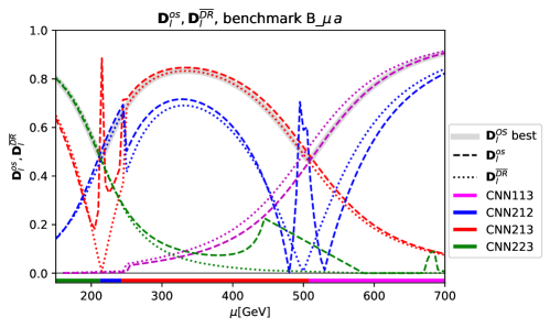
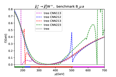
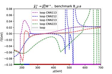
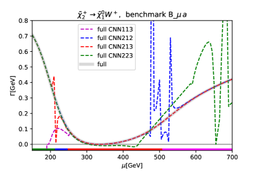
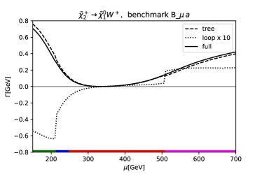
Figure 1: Decay width for $\tilde{\chi}_{2}^{+}\to\tilde{\chi}_{1}^{0}W^{+}$ as a function of $\mu$ in benchmark scenario B_$\mu\,a$, see Tab. 1, with $M_{1}=200\,\,\mathrm{GeV}$, $M_{2}=500\,\,\mathrm{GeV}$, $\tan\beta=10$. Shown are the four “best RS” in this range of parameters (see text). The upper plot shows the (“naturally normalized”) determinants $\mathbf{D}^{\smash{\overline{\mathrm{DR}}}}_{l}$ (dotted) and $\mathbf{D}^{\mathrm{os}}_{l}$ (dashed), see Eq. (99). The middle left (right) figure shows the tree (the loop plus real photon emission) results. The bottom left figure shows the full NLO decay widths obtained summing results shown in the middle figures. The bottom right figure shows the tree, loop and full results in the “best” RS for every parameter point. The horizontal colored bar shows the best RS for the corresponding value of $\mu$, following the same color coding as the curves: CNN₂₂₃ for $\mu\leq 210\,\,\mathrm{GeV}$ (green), CNN₂₁₂ for $215\,\,\mathrm{GeV}\leq\mu\leq 245\,\,\mathrm{GeV}$ (blue), CNN₂₁₃ for $250\,\,\mathrm{GeV}\leq\mu\leq 505\,\,\mathrm{GeV}$ (red), CNN₁₁₃ for $510\,\,\mathrm{GeV}\leq\mu$ (pink).

The next benchmark scenario B_$\mu\,b$ differs from B_$\mu\,a$ by the sign of $M_{1}$, i.e. we set $-200\,\,\mathrm{GeV}=M_{1}$, $M_{2}=500\,\,\mathrm{GeV}$, while $\mu$ varies from $150\,\,\mathrm{GeV}$ to $700\,\,\mathrm{GeV}$. In Fig. 2 we show the results for the same decay width as in Fig. 1, $\Gamma(\tilde{\chi}_{2}^{+}\to\tilde{\chi}_{1}^{0}W^{+})$ as a function of $\mu$ with the same arrangement of the plots. The upper plot shows the selection of the “best RS”, where again the horizontal colored bar indicates this best RS for the corresponding value of $\mu$: CNN₁₃₄ for $\mu\leq 195\,\,\mathrm{GeV}$ (green), CNN₂₁₂ for $200\,\,\mathrm{GeV}\leq\mu\leq 230\,\,\mathrm{GeV}$ (blue), CNN₁₁₄ for $235\,\,\mathrm{GeV}\leq\mu\leq 290\,\,\mathrm{GeV}$ (cyan), CNN₂₁₃ for $295\,\,\mathrm{GeV}\leq\mu\leq 505\,\,\mathrm{GeV}$ (red), CNN₁₁₃ for $510\,\,\mathrm{GeV}\leq\mu$ (pink). These selections partially agree with the scheme selected in B_$\mu\,a$, but also some schemes are chosen that do not appear in the previous scenario. As in B_$\mu\,a$ the selected best scheme has determinants larger than $\sim 0.5$, indicating that the counter terms can be determined reliably.

Overall, the result is qualitatively the same as for B_$\mu\,a$: the selected RS yields a stable tree-level result, stable loop corrections and a smooth and stable full one-loop result is obtained. For the negative sign of $\mu$ the tree-level coupling does not possess the accidental zero crossing, yielding decay widths always larger than $\sim 0.1\,\,\mathrm{GeV}$.

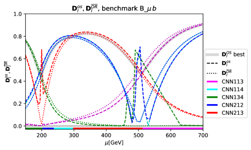
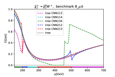
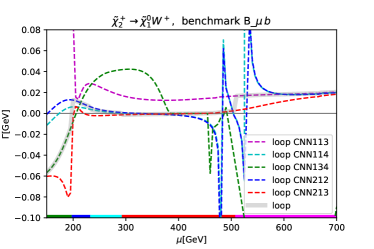
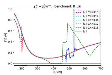
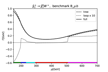
Figure 2: Decay width for $\tilde{\chi}_{2}^{+}\to\tilde{\chi}_{1}^{0}W^{+}$ as a function of $\mu$ in benchmark scenario B_$\mu\,b$, see Tab. 1, with $M_{1}=-200\,\,\mathrm{GeV}$, $M_{2}=500\,\,\mathrm{GeV}$, $\tan\beta=10$. The plots show the same quantities as in Fig. 1. Shown are the five “best RS” in this range of parameters (see text). The horizontal colored bar shows the best RS for the corresponding value of $\mu$, following the same color coding as the curves: CNN₁₃₄ for $\mu\leq 195\,\,\mathrm{GeV}$ (green), CNN₂₁₂ for $200\,\,\mathrm{GeV}\leq\mu\leq 230\,\,\mathrm{GeV}$ (blue), CNN₁₁₄ for $235\,\,\mathrm{GeV}\leq\mu\leq 290\,\,\mathrm{GeV}$ (cyan), CNN₂₁₃ for $295\,\,\mathrm{GeV}\leq\mu\leq 505\,\,\mathrm{GeV}$ (red), CNN₁₁₃ for $510\,\,\mathrm{GeV}\leq\mu$ (pink).

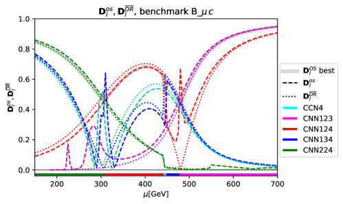
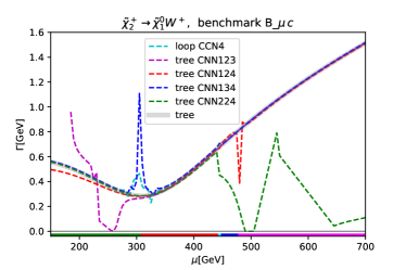
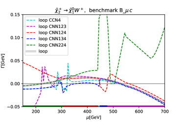
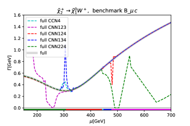
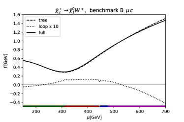
Figure 3: Decay width for $\tilde{\chi}_{2}^{+}\to\tilde{\chi}_{1}^{0}W^{+}$ as a function of $\mu$ in benchmark scenario B_$\mu\,c$, see Tab. 1, with $M_{1}=500\,\,\mathrm{GeV}$, $M_{2}=200\,\,\mathrm{GeV}$, $\tan\beta=10$. Shown are the five “best RS” in this range of parameters (see text). The plots show the same quantities as in Fig. 1. The horizontal colored bar shows the best RS for the corresponding value of $\mu$, following the same color coding as the curves: CNN₂₂₄ for $\mu\leq 305\,\,\mathrm{GeV}$ (green), CNN₁₂₄ for $310\,\,\mathrm{GeV}\leq\mu\leq 440\,\,\mathrm{GeV}$ (red), CCN₄ for $445\,\,\mathrm{GeV}\leq\mu\leq 445\,\,\mathrm{GeV}$ (cyan), CNN₁₂₃ for $480\,\,\mathrm{GeV}\leq\mu$ (pink).

We finish the numerical analysis of the variation of $\mu$ with the benchmark scenario B_$\mu\,c$, see Tab. 1, where the hierarchy of $M_{1}$ and $M_{2}$ is inverted w.r.t. B_$\mu\,a$: $500\,\,\mathrm{GeV}=M_{1}>M_{2}=200\,\,\mathrm{GeV}$ and $\tan\beta=10$, while $\mu$ is varied as before from $150\,\,\mathrm{GeV}$ to $700\,\,\mathrm{GeV}$. The results are shown in Fig. 3, with the same ordering of plots as in Fig. 1. The overall result is the same as before: the automatically selected benchmark scenario exhibits a smooth behavior, while each RS shown exhibits irregular behavior in a parameter space, where it is not selected.

In general “similar” RS as in B_$\mu\,a$ are selected: for small $\mu$ $\mbox{CNN}_{224}$ is chosen here, whereas in B_$\mu\,a$ $\mbox{CNN}_{223}$ had been selected, reflecting the inverted hierarchy of $M_{1}$ and $M_{2}$. Similarly, for large $\mu$ now $\mbox{CNN}_{123}$ is selected, whereas for B_$\mu\,a$ it was $\mbox{CNN}_{113}$, again reflecting the inverted hierarchy. In this benchmark scenario one can also observe that, albeit only for a small part of the parameter space, a CCN scheme, $\mbox{CCN}_{4}$, is selected for $\mu\sim 450\,\,\mathrm{GeV}$, where all CNN schemes turn bad. This is due to a “level crossing” of $\tilde{\chi}_{2}^{0}$ and $\tilde{\chi}_{3}^{0}$, which occurs for slightly different values of $\mu$ when the masses are computed with either the $\smash{\overline{\mathrm{DR}}}$ parameters or the $\mathrm{OS}$ parameters, i.e. reflected in $\mathbf{D}_{l}^{\smash{\overline{\mathrm{DR}}}}$ and $\mathbf{D}_{l}^{\mathrm{os}}$, respectively. Consequently, the best value of $\min\left\{\mathbf{D}_{l}^{\mathrm{os}},\mathbf{D}_{l}^{\smash{\overline{\mathrm{DR}}}}\right\}$ changes from $\mbox{CNN}_{124}$ to $\mbox{CNN}_{134}$ for different values of $\mu$, leading to a small region in-between where $\min\left\{\mathbf{D}_{l}^{\mathrm{os}},\mathbf{D}_{l}^{\smash{\overline{\mathrm{DR}}}}\right\}\sim 0.3$ and $\mbox{CCN}_{4}$ is selected.

4.3 Variation of $M_{1}$

In this subsection we demonstrate that our proposed method for the selection of an RS also works for the variation of the “genuine neutralino mass parameter”, $M_{1}$. The results are shown for the two benchmark scenarios B_$M_{1}\,a$ and B_$M_{1}\,b$, see Tab. 1, in Figs. 4 and 5, respectively. The plots in the two figures show the same quantities as in Fig. 1. The two scenarios differ in the hierarchy of $M_{2}$ and $\mu$, where in the first (second) scenario we have chosen $M_{2}=200(500)\,\,\mathrm{GeV}$ and $\mu=500(200)\,\,\mathrm{GeV}$.

The overall results are found as for the variation of $\mu$, see Sect. 4.2. The selected determinant, as shown in the upper rows of Figs. 4 and 5, become smallest for $M_{1}\approx M_{2}$, but do not go below $\sim 0.30$. For the rest of the parameter space the best determinant is above $\sim 0.47$. For B_$M_{1}\,a$ five schemes, all of type CNN, are selected, while for B_$M_{1}\,b$ only four schemes are automatically chosen, also all of type CNN. The different choices reflect, similar to the case discussed in Sect. 4.2, the two different hierarchies of $M_{2}$ and $\mu$.

Each of the schemes shows good behavior, where it is selected. The relative size of the “selected higher-order corrections” does not exceed $\sim 15\%$ and mostly stays below $\sim 5\%$. The only exceptions occur where the Born contribution vanishes due to a zero crossing of the respective coupling, as found in B_$M_{1}\,a$ for $M_{1}\sim 200\,\,\mathrm{GeV}$. The final result, as shown in the lower right plots of Figs. 4 and 5, are smooth curves with a reliable higher-order correction. Little kinks in the tree-level result, caused by a change of the OS values of the input parameters (see, e.g., Fig. 5 at $M_{1}\sim 190\,\,\mathrm{GeV}$) are smoothed out in the full one-loop result.

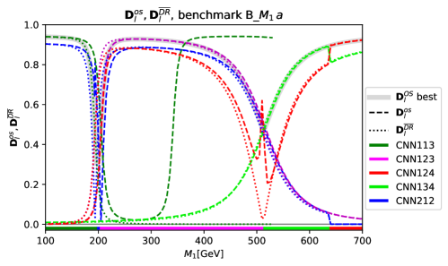
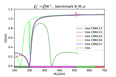
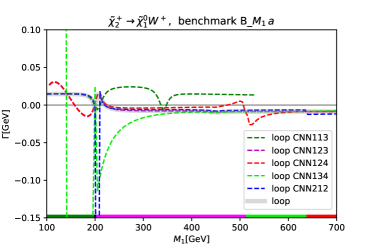
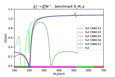
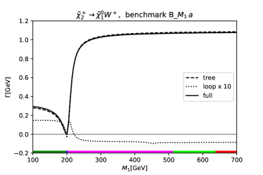
Figure 4: Decay width for $\tilde{\chi}_{2}^{+}\to\tilde{\chi}_{1}^{0}W^{+}$ as a function of $M_{1}$ in benchmark scenario B_$M_{1}\,a$, see Table 1, with $M_{2}=200\,\,\mathrm{GeV}$, $\mu=500\,\,\mathrm{GeV}$, $\tan\beta=10$. Shown are the five “best RS” in this range of parameters (see text). The plots show the same quantities as in Fig. 1. The horizontal colored bar shows the best RS for the corresponding value of $M_{1}$, following the same color coding as the curves: CNN₁₁₃ for $M_{1}\leq 195\,\,\mathrm{GeV}$, CNN₂₁₂ for $200\,\,\mathrm{GeV}\leq M_{1}\leq 200\,\,\mathrm{GeV}$, CNN₁₂₃ for $205\,\,\mathrm{GeV}\leq M_{1}\leq 510\,\,\mathrm{GeV}$, CNN₁₃₄ for $515\,\,\mathrm{GeV}\leq M_{1}\leq 635\,\,\mathrm{GeV}$, CNN₁₂₄ for $640\,\,\mathrm{GeV}\leq M_{1}$.

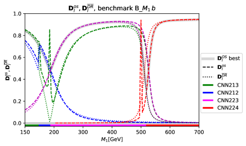
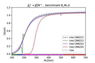
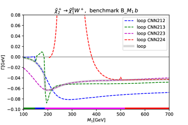
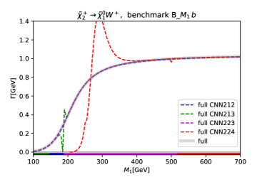
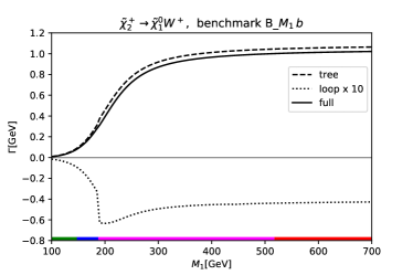
Figure 5: Decay width for $\tilde{\chi}_{2}^{+}\to\tilde{\chi}_{1}^{0}W^{+}$ as a function of $M_{1}$ in benchmark scenario B_$M_{1}\,b$, see Table 1, with $M_{2}=500\,\,\mathrm{GeV}$, $\mu=200\,\,\mathrm{GeV}$, $\tan\beta=10$. Shown are the four “best RS” in this range of parameters (see text). The plots show the same quantities as in Fig. 1. The horizontal colored bar shows the best RS for the corresponding value of $M_{1}$, following the same color coding as the curves: CNN₂₁₃ for $M_{1}\leq 145\,\,\mathrm{GeV}$, CNN₂₁₂ for $150\,\,\mathrm{GeV}\leq M_{1}\leq 185\,\,\mathrm{GeV}$, CNN₂₂₃ for $190\,\,\mathrm{GeV}\leq M_{1}\leq 515\,\,\mathrm{GeV}$, CNN₂₂₄ for $520\,\,\mathrm{GeV}\leq M_{1}$.

4.4 Variation of $M_{2}$

We finish the investigation of all possible different mass hierarchies in the chargino/neutralino sector with an analysis of the benchmark scenarios with varied $M_{2}$. The results are shown for the three benchmark scenarios B_$M_{2}\,a$, B_$M_{2}\,b$ and B_$M_{1}\,c$, see Tab. 1, in Figs. 6  7 and 8, respectively. The plots in the three figures show the same quantities as in Fig. 1. The three scenarios differ in the hierarchy and sign of $M_{1}$ and $\mu$, where in the first (second, third) scenario we have chosen $M_{2}=200(-200,500)\,\,\mathrm{GeV}$ and $\mu=500(500,200)\,\,\mathrm{GeV}$.

In principle, the overall results are found as for the variation of $\mu$ and $M_{1}$, see Sect. 4.2 and 4.3. However, in the benchmark scenario with negative $M_{1}$ a “discontinuous feature” in $\Gamma(\tilde{\chi}_{2}^{+}\to\tilde{\chi}_{1}^{0}W^{+})$ can be observed at $M_{2}\sim 200\,\,\mathrm{GeV}$. At this mass value a “level crossing” of $\tilde{\chi}_{1}^{0}$ and $\tilde{\chi}_{2}^{0}$ takes place. For $M_{2}\;\raisebox{-3.00003pt}{$\stackrel{{\scriptstyle\displaystyle<}}{{\sim}}$}\;200\,\,\mathrm{GeV}$ the $\tilde{\chi}_{1}^{0}$ ($\tilde{\chi}_{2}^{0}$) has wino (bino) character, whereas for $M_{2}\;\raisebox{-3.00003pt}{$\stackrel{{\scriptstyle\displaystyle>}}{{\sim}}$}\;200\,\,\mathrm{GeV}$ this changes to bino (wino) character. The $\tilde{\chi}_{2}^{\pm}-\tilde{\chi}_{1}^{0}-W$ coupling changes from higgsino-higgsino-gauge to wino-wino-gauge coupling, where the former is substantially larger than the latter, resulting in the strong drop of the decay width at $M_{2}\sim 200\,\,\mathrm{GeV}$. A similar pattern is observed at $\sim 200\,\,\mathrm{GeV}$ in the B_$M_{1}\,a$ benchmark scenario, where also a strong, but continuous increase of the decay rate can be observed. The difference between B_$M_{2}\,b$ and B_$M_{1}\,a$ is the ${{\cal CP}}$ character of the $\tilde{\chi}_{1}^{0}$ and $\tilde{\chi}_{2}^{0}$. The negative value of $M_{1}$ in the scenario B_$M_{2}\,b$ results in opposite values for the intrinsic ${{\cal CP}}$-parity of the two neutralinos, preventing a mixture of the two particles (we assume ${{\cal CP}}$-conservation throughout the paper). This results in a sharp transition at $M_{1}=M_{2}$. On the other hand, in scenario B_$M_{1}\,a$ the two states have the same intrinsic ${{\cal CP}}$ parities and can mix, resulting in a smooth transition. This is also reflected in the mass patterns of the neutralinos, as shown in Fig. 12, see the left plot in the second (fourth) row for B_$M_{2}\,b$ (B_$M_{1}\,a$). Correspondingly, the “best RS” changes from $\mbox{CNN}_{123}$ for $M_{2}\;\raisebox{-3.00003pt}{$\stackrel{{\scriptstyle\displaystyle<}}{{\sim}}$}\;200\,\,\mathrm{GeV}$ to $\mbox{CNN}_{113}$, such that always one wino-like state (the $\tilde{\chi}_{1}^{\pm}$), a higgsino-like state (the $\tilde{\chi}_{3}^{0}$) and a bino-like state (either $\tilde{\chi}_{2}^{0}$ for $M_{2}\;\raisebox{-3.00003pt}{$\stackrel{{\scriptstyle\displaystyle<}}{{\sim}}$}\;200\,\,\mathrm{GeV}$, or $\tilde{\chi}_{1}^{0}$ for $M_{2}\;\raisebox{-3.00003pt}{$\stackrel{{\scriptstyle\displaystyle>}}{{\sim}}$}\;200\,\,\mathrm{GeV}$) is renormalized OS. In order to demonstrate this level crossing, in the lower right plot of Fig. 7 we show the results for $\Gamma(\tilde{\chi}_{2}^{+}\to\tilde{\chi}_{j}^{0}W)$ (tree, loop ($\times 10$) and full) for $j=1,2$. It can clearly be observed that by switching from $j=1$ to $j=2$ at $M_{2}\sim 200\,\,\mathrm{GeV}$ effectively smooth results are obtained for the decay width as a function of $M_{2}$.

As stated above, in general the overall results for the variation of $M_{2}$ are found effectively identical as for the variation of $\mu$ and $M_{1}$. The selected determinant, as shown in the upper rows of Figs. 6, 7 and 8, become smallest for $M_{1}\approx M_{2}$, but do not go below $\sim 0.30$. For the rest of the parameter space the best determinant is above $\sim 0.46$. For B_$M_{2}\,a$ four schemes, all of type CNN, are selected, for B_$M_{2}\,b$ (the scenario with negative $M_{1}$), four schemes are selected while for B_$M_{2}\,c$ only three schemes are automatically chosen, all of them are of type CNN. The different choices reflect, similar to the case discussed in Sect. 4.2, the two different hierarchies of $M_{1}$ and $\mu$.

Each of the schemes shows good behavior, where it is selected. The relative size of the “selected higher-order corrections” does not exceed $\sim 15\%$ and mostly stays below $\sim 10\%$. As before, the only exceptions occur where the Born contribution vanishes due to a zero crossing of the respective coupling, as for instance $M_{2}\sim M_{1}$ in benchmark B_$M_{2}\,a$. The final result, as shown in the lower right plots of Figs. 6, 7 and 8, are smooth curves with a reliable higher-order correction (taking into account the level crossing in B_$M_{2}\,b$).

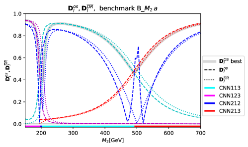
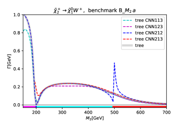
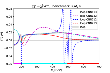
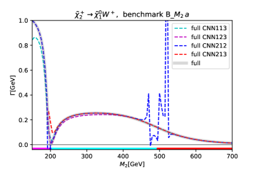
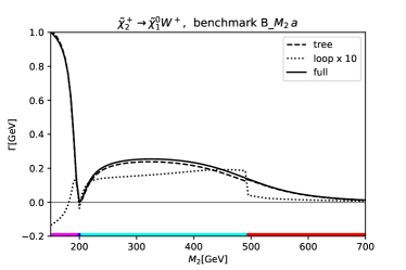
Figure 6: Decay width for $\tilde{\chi}_{2}^{+}\to\tilde{\chi}_{1}^{0}W^{+}$ as a function of $M_{2}$ in benchmark scenario B_$M_{2}\,a$, see Tab. 1, with $M_{1}=200\,\,\mathrm{GeV}$, $\mu=500\,\,\mathrm{GeV}$, $\tan\beta=10$. Shown are the four “best RS” in this range of parameters (see text). The plots show the same quantities as in Fig. 1. The horizontal colored bar shows the best RS for the corresponding value of $M_{2}$, following the same color coding as the curves: CNN₁₂₃ for $M_{2}\leq 195\,\,\mathrm{GeV}$, CNN₂₁₂ for $200\,\,\mathrm{GeV}\leq M_{2}\leq 200\,\,\mathrm{GeV}$, CNN₁₁₃ for $205\,\,\mathrm{GeV}\leq M_{2}\leq 490\,\,\mathrm{GeV}$, CNN₂₁₃ for $495\,\,\mathrm{GeV}\leq M_{2}$.

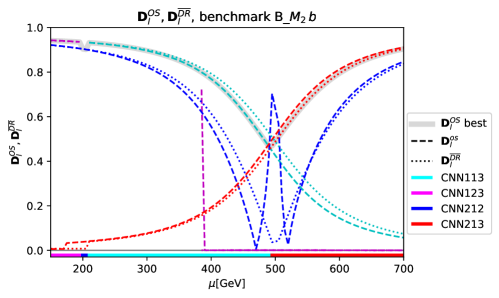
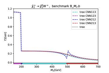
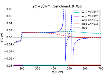
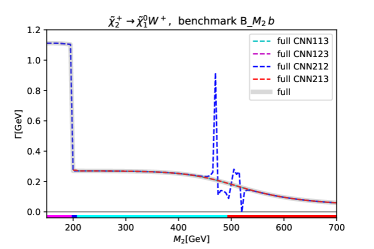
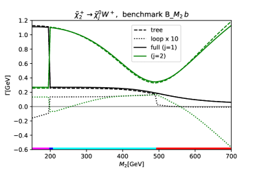
Figure 7: Decay width for $\tilde{\chi}_{2}^{+}\to\tilde{\chi}_{1}^{0}W^{+}$ as a function of $M_{2}$ in benchmark scenario B_$M_{2}\,b$, see Tab. 1, with $M_{1}=-200\,\,\mathrm{GeV}$, $\mu=500\,\,\mathrm{GeV}$, $\tan\beta=10$. Shown are the four “best RS” in this range of parameters (see text). The plots show the same quantities as in Fig. 1. In the lower right plot we show the results for $\Gamma(\tilde{\chi}_{\ }^{+}\to\tilde{\chi}_{j}^{0}W^{+}$ for $j=1,2$ (see text). The horizontal colored bar shows the best RS for the corresponding value of $M_{2}$, following the same color coding as the curves: CNN₁₂₃ for $M_{2}\leq 195\,\,\mathrm{GeV}$, CNN₂₁₂ for $200\,\,\mathrm{GeV}\leq M_{2}\leq 205\,\,\mathrm{GeV}$, CNN₁₁₃ for $210\,\,\mathrm{GeV}\leq M_{2}\leq 490\,\,\mathrm{GeV}$, CNN₂₁₃ for $495\,\,\mathrm{GeV}\leq M_{2}$.

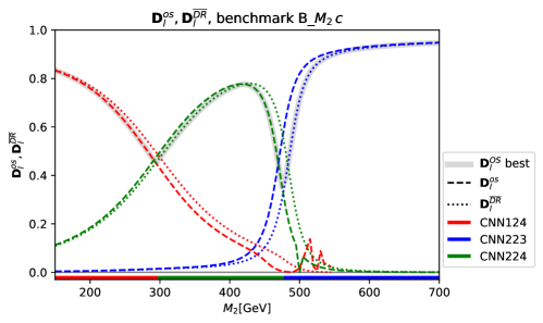
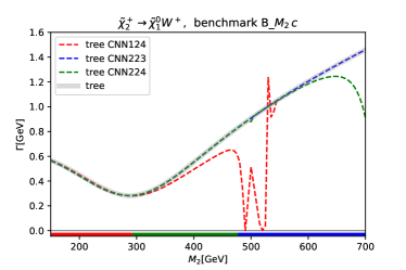
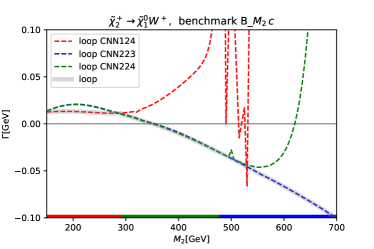
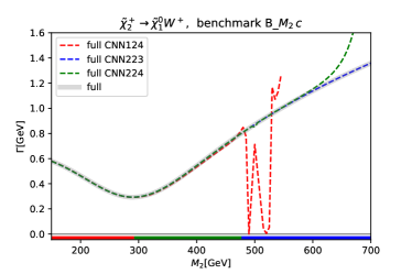
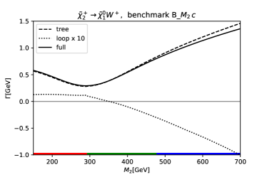
Figure 8: Decay width for $\tilde{\chi}_{2}^{+}\to\tilde{\chi}_{1}^{0}W^{+}$ as a function of $M_{2}$ in benchmark scenario B_$M_{2}\,c$, see Tab. 1, with $M_{1}=500\,\,\mathrm{GeV}$, $\mu=300\,\,\mathrm{GeV}$, $\tan\beta=10$. Shown are the three “best RS” in this range of parameters (see text). The plots show the same quantities as in Fig. 1. The horizontal colored bar shows the best RS for the corresponding value of $M_{2}$, following the same color coding as the curves: CNN₁₂₄ for $M_{2}\leq 290\,\,\mathrm{GeV}$, CNN₂₂₄ for $295\,\,\mathrm{GeV}\leq M_{2}\leq 475\,\,\mathrm{GeV}$, CNN₂₂₃ for $480\,\,\mathrm{GeV}\leq M_{2}$.

Additional figures with other decay widths involving $Z$ and $h$ in the final state ($\Gamma(\tilde{\chi}_{4}^{0}\to\tilde{\chi}_{1}^{0}h)$, $\Gamma(\tilde{\chi}_{4}^{0}\to\tilde{\chi}_{1}^{0}Z)$) can be found in appendix B.

For the benchmark scenario B_$M_{2}\,a$ we also discuss another physics case: having one (or more) external charged particles makes it desirable to have them renormalized OS. This ensures the cancellation of IR divergences to all orders. If, on the other hand, such a RS cannot be chosen, chargino mass shifts are employed, see the discussion in Sect. 3.1.  From a perturbation theory point of view both solutions are acceptable. However, a full OS renormalization of external charged particles still appears preferred.

In Fig. 9 we show the results, analogous to Fig. 6 where all benchmark scenarios were allowed to be chosen, for the decay $\tilde{\chi}_{2}^{+}\to\tilde{\chi}_{1}^{0}W^{+}$, but now enforcing the $\tilde{\chi}_{2}^{\pm}$ to be renormalized OS. In Fig. 6 two out of the four chosen RS had the $\tilde{\chi}_{2}^{\pm}$ not renormalized OS ($\mbox{CNN}_{113}$ and $\mbox{CNN}_{123}$), which are now forbidden. Forcing the $\tilde{\chi}_{2}^{\pm}$ to be renormalized OS now results in two CCN to be selected ($\mbox{CCN}_{1}$ and $\mbox{CCN}_{2}$), along with the already previously chosen $\mbox{CNN}_{212}$ and $\mbox{CNN}_{213}$. However, also the $M_{2}$ values where the latter ones are selected change strongly w.r.t. Fig. 6. However, also in this case the selected determinant is larger than $\sim 0.30$. The overall behavior of the selected loop corrections and the final obtained decay width as shown in Fig. 9 is nearly identical to the result shown in Fig. 6, included for a better comparison as cyan line in the lower right plot of Fig. 9, showing the “best” full result. For $M_{2}>490\,\,\mathrm{GeV}$ the chosen RS are the same, i.e. leading to identical results, while for $M_{2}\leq 490\,\,\mathrm{GeV}$ the difference is too small to be appreciated, except for $M_{2}\sim 440\,\,\mathrm{GeV}$, where a slight difference can be observed. This demonstrates that the overall idea to choose a “good RS” also works in case of a restricted allowed set of RS (in this case forcing the $\tilde{\chi}_{2}^{\pm}$ to be renormalized OS to avoid problems with the cancellation of IR divergences).

Similarly, in Fig. 10 we show the results for the decay $\tilde{\chi}_{4}^{0}\to\tilde{\chi}_{1}^{+}W^{-}$ in the benchmark scenario B_$M_{2}\,a$, and with the $\tilde{\chi}_{1}^{\pm}$ forced to be renormalized OS. Now one CCN scheme ($\mbox{CCN}_{1}$) and two CNN schemes ($\mbox{CNN}_{123}$ and $\mbox{CNN}_{113}$) are selected. As in the case of the $\tilde{\chi}_{2}^{\pm}$ forced to be renormalized OS, also here we find the smallest selected determinant larger than $\sim 0.25$, and in the end an effectively smooth loop-corrected decay width, as can be observed the lower right plot of Fig. 10. Only at $M_{2}\sim 550\,\,\mathrm{GeV}$ a very small kink due to the change from one $\mbox{CNN}_{113}$ to $\mbox{CCN}_{1}$ can be observed. As in the previous figure, for sake of comparison, we also include the “best” full results as obtained without any restrictions on the set of allowed RS, shown as cyan line in the lower right plot. Only a tiny difference can be observed for $M_{2}$ between $500$ and $540\,\,\mathrm{GeV}$, as expected from different renormalization schemes, resulting in differences at the two-loop level.

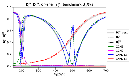
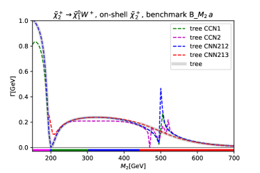
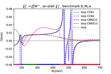
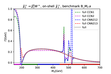
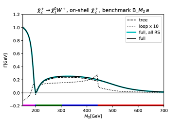
Figure 9: Decay width for $\tilde{\chi}_{2}^{+}\to\tilde{\chi}_{1}^{0}W^{+}$ as a function of $M_{2}$ in benchmark scenario B_$M_{2}\,a$, see Tab. 1, with $M_{1}=200\,\,\mathrm{GeV}$, $\mu=500\,\,\mathrm{GeV}$, $\tan\beta=10$. Shown are the four “best RS” in this range of parameters, where the $\tilde{\chi}_{2}^{\pm}$ is forced to be renormalized OS. The plots show the same quantities as in Fig. 1. Also shown in the lower right plot is the “full” result with all RS allowed (cyan line, reproduced from the lower right plot of Fig. 6). The horizontal colored bar shows the best RS for the corresponding value of $M_{2}$, following the same color coding as the curves: CCN₂ for $M_{2}\leq 195\,\,\mathrm{GeV}$, CNN₂₁₂ for $200\,\,\mathrm{GeV}\leq M_{2}\leq 200\,\,\mathrm{GeV}$, CCN₁ for $205\,\,\mathrm{GeV}\leq M_{2}\leq 300\,\,\mathrm{GeV}$, CNN₂₁₂ for $305\,\,\mathrm{GeV}\leq M_{2}\leq 440\,\,\mathrm{GeV}$, CNN₂₁₃ for $445\,\,\mathrm{GeV}\leq M_{2}$.

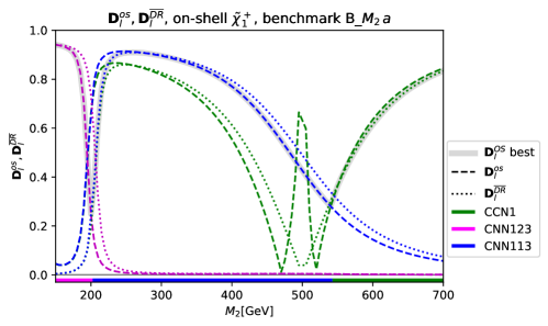
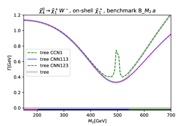
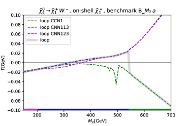
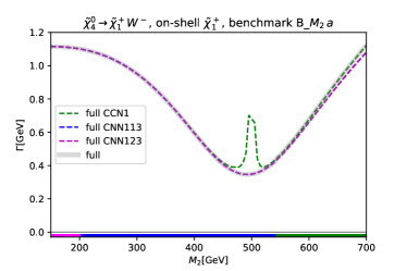
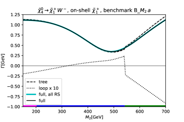
Figure 10: Decay width for $\tilde{\chi}_{4}^{0}\to\tilde{\chi}_{1}^{+}W^{-}$ as a function of $M_{2}$ in benchmark scenario B_$M_{2}\,a$, see Tab. 1, with $M_{1}=200\,\,\mathrm{GeV}$, $\mu=500\,\,\mathrm{GeV}$, $\tan\beta=10$. Shown are the four “best RS” in this range of parameters, where the $\tilde{\chi}_{1}^{\pm}$ is forced to be renormalized OS. The plots show the same quantities as in Fig. 1. Also shown in the lower right plot is the “full” result with all RS allowed (cyan line). The horizontal colored bar shows the best RS for the corresponding value of $M_{2}$, following the same color coding as the curves: CNN₁₂₃ for $M_{2}\leq 200\,\,\mathrm{GeV}$, CNN₁₁₃ for $205\,\,\mathrm{GeV}\leq M_{2}\leq 540\,\,\mathrm{GeV}$, CCN₁ for $545\,\,\mathrm{GeV}\leq M_{2}$.

4.5 Variation of two parameters

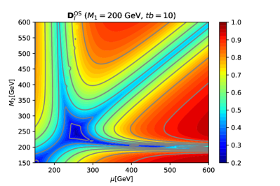
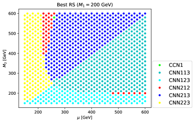
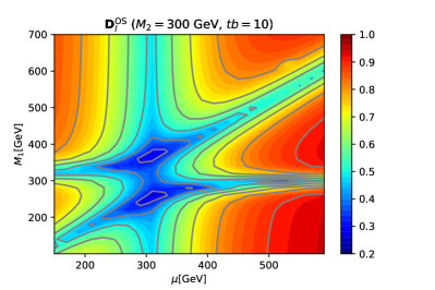
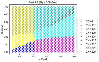
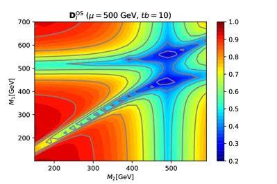
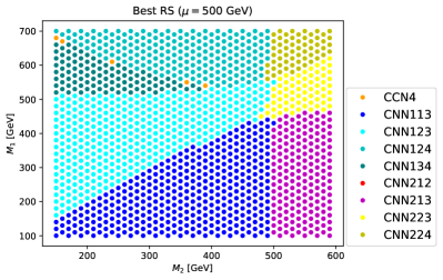
Figure 11: The normalized determinant $\mathbf{D}^{\mathrm{OS}}_{l}$, see Eq. (100), for the best RS (left) and the corresponding RS (right) in: the $\mu-M_{2}$ plane for $M_{1}=200\,\,\mathrm{GeV}$ (top), the $\mu-M_{1}$ plane for $M_{2}=300\,\,\mathrm{GeV}$ (middle), kand in the $M_{2}-M_{1}$ plane for $\mu=500\,\,\mathrm{GeV}$ (bottom). In all scenarios $\tan\beta=10$.

We finish our analysis of the automated RS choice with the results for 2-dimensional planes. In the previous subsections we demonstrated that our proposed algorithm is capable of selecting a good RS, resulting in a smooth result over the analyzed one-dimensional parameter interval. One might suspect that simple cuts or rules could yield a similarly good result. The investigation of the 2-dimensional planes demonstrates that this is not the case. In Fig. 11 we present the normalized determinant $\mathbf{D}^{\mathrm{OS}}_{l}$, see Eq. (100), or the best RS (left) and the corresponding RS (right) in: the $\mu-M_{2}$ plane for $M_{1}=200\,\,\mathrm{GeV}$ (top), the $\mu-M_{1}$ plane for $M_{2}=300\,\,\mathrm{GeV}$ (middle), and in the $M_{2}-M_{1}$ plane for $\mu=500\,\,\mathrm{GeV}$ (bottom), all for $\tan\beta=10$. In all scenarios $\tan\beta=10$. The color coding indicates the size of the maximum normalized determinant (left) and the choice of the chosen RS (right). In the left column one can observe that even in the most “critical” situations when all three mass parameters are of similar size, the largest determinant does not go below $\sim 0.23$. For two mass parameters close in range, the determinant only goes down to about $\sim 0.4$ for $\mu\sim M_{2}$ and about $\sim 0.3$ for $M_{1}\sim M_{2}$. In the right column of Fig. 11, where we indicate the selected RS, one can observe that a multitude of schemes is chosen all over the planes. No simple rules or cuts can reproduce the pattern of the selected RS. This demonstrates the power of our new proposed algorithm, which cannot be reproduced by simple selection cuts.

5 Conclusions

The explorations of models beyond the Standard Model (BSM) naturally involve scans over the BSM parameters. On the other hand, high precision predictions require calculations at the loop-level and thus a renormalization of (some of) the BSM parameters. Often many choices for the renormalization scheme (RS) are possible. This concerns the choice of the set of to-be-renormalized parameters out of a larger set of BSM parameters, but can also concern the type of renormalization condition which is chosen for a specific parameter. A given RS can be well suited to yield “stable” and “well behaved” higher-order corrections in one part of the BSM parameter space, but can fail completely in other parts. Such a failure may not even be noticed numerically if an isolated parameter point (e.g. in a large scan) is investigated. Consequently, the exploration of BSM models requires a choice of a good RS before the calculation is performed.

In this paper we proposed a new method how such a situation can be avoided, i.e. how a “good” RS can be chosen before performing the calculation. This new method is based on the properties of the transformation matrix that connects the various counter terms with the underlying parameters. The “best RS” is chosen as the one that (for the parameter point under investigation) possesses the largest (normalized) determinant of the transformation matrix, a quantity that can be evaluated for all RS under consideration before the actual higher-order calculation is performed. This allows a point-by-point test of all “available” or “possible” RS, and the “best” one can be chosen to perform the calculation.

Our idea is designed to work in all cases of RS choices (in BSM models). In order to demonstrate its feasibility and power, we concentrated on a more specific question: in many BSM models one can be faced with the situation that one has $m$ underlying Lagrangian parameters and $n>m$ particles or particle masses that can be renormalized on-shell (OS). The calculation of the production and/or decay of BSM particles naturally requires OS renormalizations of the particles involved. Each choice of $m$ particles renormalized OS defines an $\mbox{RS}_{l}$, of which we have $N$ in total. We have demonstrated how out of these $N$ $\mbox{RS}_{l}$ one can choose the “best” $\mbox{RS}_{L}$. Starting from $\smash{\overline{\mathrm{DR}}}$ input parameters we provided a detailed and “model independent” description how OS parameter can be derived. This can be done in one step, where the OS masses and parameters are evaluated from the original $\smash{\overline{\mathrm{DR}}}$ parameters, the “semi-OS” scheme. This can also be done in two steps, where in the second step after the semi-OS scheme the OS masses are derived from OS parameters, the “full-OS” scheme. In our numerical evaluation we have concentrated on the latter.

The numerical examples have been performed within the MSSM, concretely in the sector of charginos and neutralinos, the supersymmetric (SUSY) partners of the SM gauge bosons and the 2HDM-like Higgs sector. The sector is controlled by the three mass parameters $M_{1}$, $M_{2}$ and $\mu$, as well as $\tan\beta$. Three out of the six chargino/neutralino masses can be renormalized OS, whereas the other three masses receive an extra one-loop shift to yield the correct OS mass. While concentrating on the chargino/neutralino sector of the MSSM this constitutes a very specific example, we would like to stress the general applicability of our method to all types of BSM models and types of RS choices.

We have investigated eight mass hierarchies, in which two of the three mass parameters were fixed, and the third one changed continuously from very small to very large values (with $\tan\beta=10$). This ensure that all mass hierarchies the model offers are covered. We have concentrated on the RS renormalizing either one chargino ($\mbox{CNN}_{ijk}$) or two charginos ($\mbox{CCN}_{i}$) OS and left out the possibility of normalizing three neutralinos OS ($\mbox{NNN}_{ijk}$). This yielded in total 16 RS that can potentially be chosen. As physical process, we mostly concentrated on the decay width $\Gamma(\tilde{\chi}_{2}^{+}\to\tilde{\chi}_{1}^{0}W^{+})$.

For each scenario we presented five plots. The first one showed the analysis of the determinants of the transformation matrices, leading to the choice of “the best RS” before performing any actual calculation. Next we presented the tree results for all RS that are chosen in at least one parameter point in the scan, resulting in four to five RS for each benchmark scenario. The results for all RS are shown for the full parameter region for comparison (with one fixed color for each chosen RS), and we indicated which RS is best for each parameter point. One can observe that where a scheme is chosen, the tree level width behaves “well” and smoothly. On the other hand, outside the selected interval the tree-level result behaves highly irregularly, induced by the shifts in the mass matrices to obtain OS masses. Next, we presented a plot showing the “loop plus real photon emission” results with the same color coding as for the tree result. One can observe that where a scheme is chosen the loop corrections behave smoothly and the overall size stays at the level of $\sim 10\%$ or less compared to the tree-level result (exceptions are found only where the tree result goes to zero due to an accidental zero crossing of the involved tree-level coupling). As before, outside the chosen interval the loop corrections take irregular values, which sometimes even diverge, owing to a vanishing determinant. The next plot presented for each benchmark scenario showed the sum of tree and higher-order corrections, i.e. of the two previous plots. The same pattern of numerical behavior can be observed. The chosen scheme yields a reliable higher-order corrected result, whereas other schemes result in highly irregular and clearly unreliable results. This is summarized in the final plot, where we show the selected tree-level result as dashed line, the loop result as dotted (multiplied by 10 for better visibility), and the full result as solid line. The overall behavior is completely well-behaved and smooth. A remarkable feature can be observed in some cases, where the selected tree-level result has a kink, because of a change in the shift in the OS values of the involved chargino/neutralino masses, caused by the change from switching one selected RS to another. In this case, the loop corrections contain also a corresponding kink, leading to a completely smooth full one-loop result.

In a final step we have presented an analysis of the automated RS choice with the results for 2-dimensional planes. Looking only at the 1-dimensional analysis, one might suspect that simple cuts or rules could yield a similarly good result. The investigation of the 2-dimensional planes demonstrated that this is not the case. For three planes ($\mu-M_{2}$, $\mu-M_{1}$ and $M_{2}-M_{1}$) we show the value of the determinant of the chosen RS, which in effectively all cases analyzed remains above $\sim 0.3$. We furthermore showed in a separate plot the RS chosen for each point in the parameter plane. One can observe that a multitude of schemes is chosen all over the planes. No simple rules or cuts can reproduce the pattern of the selected RS. This demonstrates the power of our new proposed algorithm, which cannot be reproduced by simple selection cuts.

As next steps, we plan to apply our method to more involved calculations such as $2\to 2$ processes, as well as to Dark Matter related calculations in parameter regions with small mass splittings between various charginos/neutralinos. We will also apply the new method to the other sectors of the MSSM, where the renormalization can be even more involved than in the chargino/neutralino sector (see Refs. [40, 41, 42, 43, 44, 45, 46]). Furthermore, we intend to make our modified FeynArts/FormCalc versions public, which have been used to obtain the results presented here. On the other hand, we plan to apply our method to different types of renormalization schemes in other (types of) models. Only a method to select a reliable RS before the calculation is performed will allow a fully automated set-up of BSM higher-order calculations. We hope that our newly proposed method will enable such fully automated set-ups for BSM higher-order calculations.

Acknowledgments

We thank C. Schappacher for helpful discussions and in particular for invaluable help with the chargino mass shifts concerning the IR divergences. The work of S.H. has received financial support from the grant PID2019-110058GB-C21 funded by MCIN/AEI/10.13039/501100011033 and by “ERDF A way of making Europe”. MEINCOP Spain under contract PID2019-110058GB-C21 and in part by by the grant IFT Centro de Excelencia Severo Ochoa CEX2020-001007-S funded by MCIN/AEI/10.13039/ 501100011033.

Appendix

Appendix A Transformation matrices for the counter terms

In order to give an explicit form for the transformation matrix $\mathbf{A}_{l}^{\smash{\overline{\mathrm{DR}}}}$, Eq. (76), we order the model parameters as

$$P_{1}^{\smash{\overline{\mathrm{DR}}}}=M_{1}^{\smash{\overline{\mathrm{DR}}}},\;P_{2}^{\smash{\overline{\mathrm{DR}}}}=M_{2}^{\smash{\overline{\mathrm{DR}}}},\;P_{3}^{\smash{\overline{\mathrm{DR}}}}=\mu^{\smash{\overline{\mathrm{DR}}}}\,.$$ (A.1)

For a $\mbox{CCN}_{n}$ RS the transformation matrix $\mathbf{A}_{l}^{\smash{\overline{\mathrm{DR}}}}$ is given by

$$\mathbf{A}^{\smash{\overline{\mathrm{DR}}}}_{l} =\begin{pmatrix}0&V^{*}_{11}U^{*}_{11}&V^{*}_{12}U^{*}_{12}\\ 0&V^{*}_{21}U^{*}_{21}&V^{*}_{22}U^{*}_{22}\\ (N^{*}_{n1})^{2}&(N^{*}_{n2})^{2}&-2N^{*}_{n3}N^{*}_{n4}\end{pmatrix}~{},$$ (A.2)

with $l=1,\ldots,4$ for all possible values of $n$. For a $\mbox{CNN}_{cnn^{\prime}}$ RS the matrix $\mathbf{A}_{l}^{\smash{\overline{\mathrm{DR}}}}$ is given by

$$\mathbf{A}^{\smash{\overline{\mathrm{DR}}}}_{l} =\begin{pmatrix}0&V^{*}_{c1}U^{*}_{c1}&V^{*}_{c2}U^{*}_{c2}\\ (N^{*}_{n1})^{2}&(N^{*}_{n2})^{2}&-2N^{*}_{n3}N^{*}_{n4}\\ (N^{*}_{n^{\prime}1})^{2}&(N^{*}_{n^{\prime}2})^{2}&-2N^{*}_{n^{\prime}3}N^{*}_{n^{\prime}4}\end{pmatrix}~{},$$ (A.3)

with $l=5,\ldots,16$, corresponding to all possible combinations of $c$, $n$ and $n^{\prime}$. It is worth noticing that in Eqs. (A.2) and (A.3) the unitary matrices $\mathbf{U}$, $\mathbf{V}$ and $\mathbf{N}$ have been obtained diagonalizing the chargino and neutralino mass matrices given in terms of the $\smash{\overline{\mathrm{DR}}}$ parameters. In order to obtain $\mathbf{A}_{l}^{\mathrm{os}}$ the diagonalization matrices $\mathbf{U}$, $\mathbf{V}$ and $\mathbf{N}$ have to be computed from chargino and neutralino mass matrices given in terms of $\mathrm{os}$ parameters of the corresponding RS.

Appendix B Additional plots

In this appendix we collect additional plots that are not necessary to follow the main line of argument in the article, but may give some interesting additional information. In Fig. 12 we present the masses of the two charginos and the four neutralinos in all eight benchmark scenarios, as defined in Tab. 1. The mass plots, besides showing the masses themselves, illustrate the two different types of “level crossing”. As an example, in the upper left plot, scenario B_$M_{2}\,a$ at $M_{2}\sim 200\,\,\mathrm{GeV}$ the $\tilde{\chi}_{1}^{0}$ and $\tilde{\chi}_{2}^{0}$ have the same intrinsic ${{\cal CP}}$ parities, therefore mix with each other, and thus experience a “smooth” level crossing, as can be observed by the smooth dependence of the masses. On the other hand, in the second row left, scenario B_$M_{2}\,b$ the two neutralinos have different ${{\cal CP}}$ quantum numbers and do not mix. Consequently, they exhibit a “sharp” crossing of the two masses at $M_{2}\sim 200\,\,\mathrm{GeV}$, see also the discussion in Sect. 4.4.

In Figs. 13 and 14 we show “neutral decays” involving either the $\sim 125\,\,\mathrm{GeV}$ Higgs boson, $h$, or the $Z$ boson, $\tilde{\chi}_{4}^{0}\to\tilde{\chi}_{1}^{0}h/Z$. For these figures the benchmark scenario B_$M_{2}\,a$ has been chosen (and thus the top plots are identical to the of Fig. 6, but shown for completeness). The arrangement of plots is as in the main text, see the description in Fig. 1. These two sets of plots simply demonstrate the effectiveness of our newly proposed approach in two new decay channels, with either the $h$ or the $Z$ in the final states. The overall conclusions are as in the main text.

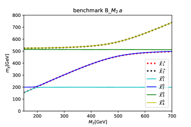
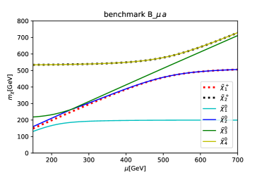
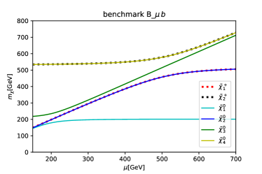
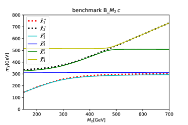
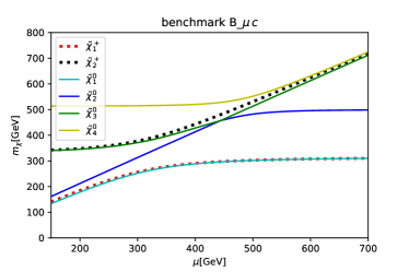
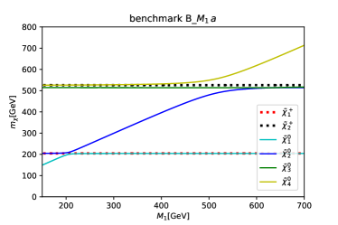
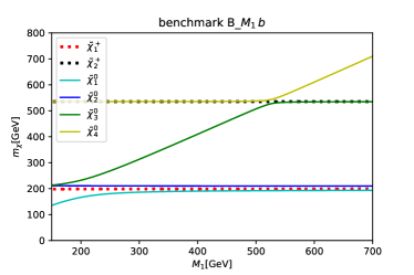
Figure 12: Masses of charginos and neutralinos in all benchmark scenarios, see Tab. 1.

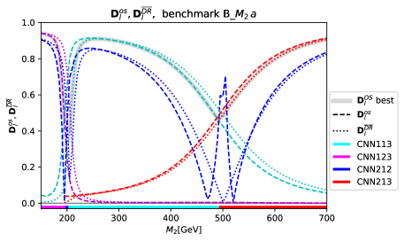
Figure 13: Decay width for $\tilde{\chi}_{4}^{0}\to\tilde{\chi}_{1}^{0}h$ as a function of $M_{2}$ in benchmark scenario B_$M_{2}\,a$, see Tab. 1, with $M_{1}=200\,\,\mathrm{GeV}$, $\mu=500\,\,\mathrm{GeV}$, $\tan\beta=10$. Shown are the four “best RS” in this range of parameters (see text). The plots show the same quantities as in Fig. 1. The horizontal colored bar shows the best RS for the corresponding value of $M_{2}$, following the same color coding as the curves: CNN₁₂₃ for $M_{2}\leq 195\,\,\mathrm{GeV}$, CNN₂₁₂ for $200\,\,\mathrm{GeV}\leq M_{2}\leq 200\,\,\mathrm{GeV}$, CNN₁₁₃ for $205\,\,\mathrm{GeV}\leq M_{2}\leq 490\,\,\mathrm{GeV}$, CNN₂₁₃ for $495\,\,\mathrm{GeV}\leq M_{2}$.

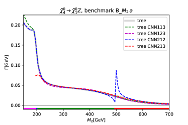
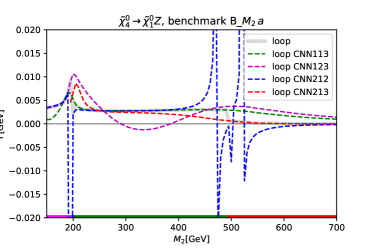
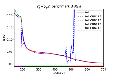
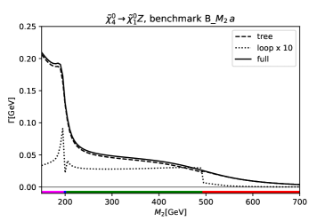
Figure 14: Decay width for $\tilde{\chi}_{4}^{0}\to\tilde{\chi}_{1}^{0}Z$ as a function of $M_{2}$ in benchmark scenario B_$M_{2}\,a$, see Tab. 1, with $M_{1}=200\,\,\mathrm{GeV}$, $\mu=500\,\,\mathrm{GeV}$, $\tan\beta=10$. Shown are the four “best RS” in this range of parameters (see text). The plots show the same quantities as in Fig. 1. The horizontal colored bar shows the best RS for the corresponding value of $M_{2}$, following the same color coding as the curves: CNN₁₂₃ for $M_{2}\leq 195\,\,\mathrm{GeV}$, CNN₂₁₂ for $200\,\,\mathrm{GeV}\leq M_{2}\leq 200\,\,\mathrm{GeV}$, CNN₁₁₃ for $205\,\,\mathrm{GeV}\leq M_{2}\leq 490\,\,\mathrm{GeV}$, CNN₂₁₃ for $495\,\,\mathrm{GeV}\leq M_{2}$.

References

- [1]
- [2] M. Bohm, H. Spiesberger and W. Hollik, Fortsch. Phys. 34 (1986), 687-751.
- [3] W. F. L. Hollik, Fortsch. Phys. 38 (1990), 165-260.
- [4] L. Altenkamp, S. Dittmaier and H. Rzehak, JHEP 09 (2017), 134 [arXiv:1704.02645 [hep-ph]].
- [5] S. Kanemura, M. Kikuchi, K. Sakurai and K. Yagyu, Phys. Rev. D 96 (2017) no.3, 035014 [arXiv:1705.05399 [hep-ph]].
- [6] M. Krause and M. Mühlleitner, JHEP 04 (2020), 083 [arXiv:1912.03948 [hep-ph]].
- [7] A. Denner, S. Dittmaier and J. N. Lang, JHEP 11 (2018), 104 [arXiv:1808.03466 [hep-ph]].
- [8] N. Baro and F. Boudjema, Phys. Rev. D 80 (2009), 076010 [arXiv:0906.1665 [hep-ph]].
- [9] N. Baro, F. Boudjema and A. Semenov, Phys. Rev. D 78 (2008), 115003 [arXiv:0807.4668 [hep-ph]].
- [10] T. Fritzsche, T. Hahn, S. Heinemeyer, F. von der Pahlen, H. Rzehak, C. Schappacher, Comput. Phys. Commun. 185 (2014) 1529 [arXiv:1309.1692 [hep-ph]].
- [11] T. Fritzsche, S. Heinemeyer, H. Rzehak, C. Schappacher, Phys. Rev. D 86 (2012) 035014 [arXiv:1111.7289 [hep-ph]].
- [12] G. Belanger, V. Bizouard, F. Boudjema and G. Chalons, Phys. Rev. D 93 (2016) no.11, 115031 [arXiv:1602.05495 [hep-ph]].
- [13] G. Bélanger, V. Bizouard, F. Boudjema and G. Chalons, Phys. Rev. D 96 (2017) no.1, 015040 [arXiv:1705.02209 [hep-ph]].
- [14] K. Ender, T. Graf, M. Muhlleitner and H. Rzehak, Phys. Rev. D 85 (2012), 075024 [arXiv:1111.4952 [hep-ph]].
- [15] T. Graf, R. Grober, M. Muhlleitner, H. Rzehak and K. Walz, JHEP 10 (2012), 122 [arXiv:1206.6806 [hep-ph]].
- [16] P. Drechsel, L. Galeta, S. Heinemeyer and G. Weiglein, Eur. Phys. J. C 77 (2017) no.1, 42 [arXiv:1601.08100 [hep-ph]].
- [17] E. Bagnaschi et al. [MasterCode], Eur. Phys. J. C 78 (2018) no.3, 256 [arXiv:1710.11091 [hep-ph]].
- [18] P. Athron et al. [GAMBIT], Eur. Phys. J. C 77 (2017) no.12, 879 [arXiv:1705.07917 [hep-ph]].
- [19] A. Chatterjee, M. Drees, S. Kulkarni and Q. Xu, Phys. Rev. D 85 (2012) 075013 [arXiv:1107.5218 [hep-ph]].
- [20] S. Heinemeyer, F. von der Pahlen, C. Schappacher, Eur. Phys. J. C 72 (2012) 1892 [arXiv:1112.0760 [hep-ph]].
- [21] S. Heinemeyer, F. von der Pahlen, C. Schappacher, arXiv:1202.0488 [hep-ph].
- [22] A. Bharucha, S. Heinemeyer, F. von der Pahlen, C. Schappacher, Phys. Rev. D 86 (2012) 075023 [arXiv:1208.4106 [hep-ph]].
- [23] A. Bharucha, S. Heinemeyer, F. von der Pahlen, Eur. Phys. J. C 73 (2013) 2629 [arXiv:1307.4237 [hep-ph]].
- [24] S. Heinemeyer, C. Schappacher, Eur. Phys. J. C 77 (2017) 9, 649 [arXiv:1704.07627 [hep-ph]].
- [25] T. Takagi, Japan J. Math. 1 (1925) 83.
- [26] T. Fritzsche, PhD thesis, Cuvillier-Verlag, Göttingen 2005, ISBN 3-86537-577-4.
-
[27]
A. Fowler, PhD thesis:
“Higher-order and CP-violating effects in the neutralino and
Higgs-boson sectors of the MSSM”,
Durham University, UK, September 2010;
A. Fowler and G. Weiglein, JHEP 1001 (2010) 108 [arXiv:0909.5165 [hep-ph]]. - [28] J. Küblbeck, M. Böhm, A. Denner, Comput. Phys. Commun. 60 (1990) 165.
- [29] T. Hahn, Comput. Phys. Commun. 140 (2001) 418 [arXiv:hep-ph/0012260].
-
[30]
T. Hahn, C. Schappacher,
Comput. Phys. Commun. 143 (2002) 54
[arXiv:hep-ph/0105349].
Program, user’s guide and model files are available via: http://www.feynarts.de . -
[31]
T. Hahn, M. Pérez-Victoria,
Comput. Phys. Commun. 118 (1999) 153
[arXiv:hep-ph/9807565].
Program and user’s guide are available via: http://www.feynarts.de/formcalc/ . - [32] T. Hahn, S. Paßehr, C. Schappacher, PoS LL2016 (2016) 068, J. Phys. Conf. Ser. 762 (2016) 1, 012065 [arXiv:1604.04611 [hep-ph]].
-
[33]
S. Heinemeyer, W. Hollik and G. Weiglein,
Comput. Phys. Commun. 124 (2000) 76
[arXiv:hep-ph/9812320];
T. Hahn, S. Heinemeyer, W. Hollik, H. Rzehak and G. Weiglein, Comput. Phys. Commun. 180 (2009) 1426;
H. Bahl, T. Hahn, S. Heinemeyer, W. Hollik, S. Paßehr, H. Rzehak and G. Weiglein, Comput. Phys. Commun. 249 (2020) 107099 [arXiv:1811.09073 [hep-ph]];
see: www.feynhiggs.de . - [34] S. Heinemeyer, W. Hollik and G. Weiglein, Eur. Phys. J. C 9 (1999) 343 [arXiv:hep-ph/9812472].
- [35] G. Degrassi, S. Heinemeyer, W. Hollik, P. Slavich and G. Weiglein, Eur. Phys. J. C 28 (2003) 133 [arXiv:hep-ph/0212020].
- [36] T. Hahn, S. Heinemeyer, W. Hollik, H. Rzehak and G. Weiglein, Phys. Rev. Lett. 112 (2014) 141801 [arXiv:1312.4937 [hep-ph]].
-
[37]
H. Bahl and W. Hollik,
Eur. Phys. J. C 76 (2016) no.9, 499
[arXiv:1608.01880 [hep-ph]];
H. Bahl, S. Heinemeyer, W. Hollik and G. Weiglein, Eur. Phys. J. C 78 (2018) no.1, 57 [arXiv:1706.00346 [hep-ph]]. - [38] H. Bahl, S. Heinemeyer, W. Hollik and G. Weiglein, Eur. Phys. J. C 80 (2020) no.6, 497 [arXiv:1912.04199 [hep-ph]].
- [39] S. Heinemeyer, F. v.d. Pahlen, proceedings of the conference “Loops and Legs in Quantum Field Theory (LL2022)”, 25 - 30 April 2022, Kloster Ettal, Germany, IFT-UAM/CSIC-22-76.
- [40] S. Heinemeyer and C. Schappacher, Eur. Phys. J. C 72 (2012), 1905 [arXiv:1112.2830 [hep-ph]].
- [41] S. Heinemeyer and C. Schappacher, Eur. Phys. J. C 72 (2012), 2136 [arXiv:1204.4001 [hep-ph]].
- [42] S. Heinemeyer and C. Schappacher, Eur. Phys. J. C 75 (2015) no.5, 198 [arXiv:1410.2787 [hep-ph]].
- [43] S. Heinemeyer and C. Schappacher, Eur. Phys. J. C 75 (2015) no.5, 230 [arXiv:1503.02996 [hep-ph]].
- [44] S. Heinemeyer and C. Schappacher, Eur. Phys. J. C 76 (2016) no.4, 220 [arXiv:1511.06002 [hep-ph]].
- [45] S. Heinemeyer and C. Schappacher, Eur. Phys. J. C 76 (2016) no.10, 535 [arXiv:1606.06981 [hep-ph]].
- [46] S. Heinemeyer and C. Schappacher, Eur. Phys. J. C 78 (2018) no.7, 536 [arXiv:1803.10645 [hep-ph]].
- [47]