Fractional Analytic QCD beyond Leading Order in timelike region

Abstract

In this paper we show that, as in the spacelike case, the inverse logarithmic expansion is applicable for all values of the argument of the analytic coupling constant. We present two different approaches, one of which is based primarily on trigonometric functions, and the latter is based on dispersion integrals. The results obtained up to the 5th order of perturbation theory, have a compact form and their acquiring is much easier than the methods that have been used before. As an example, we apply our results to study the Higgs boson decay into a $b\overline{b}$ pair.

I Introduction

The perturbative expansion in QCD works well only for estimation of the quantities in the region of large squared momentum $Q^{2}$ (here and further $Q^{2}=-q^{2}$, where $q^{2}$ – transfered momentum in the Euclidean domain for space-like processes). However, for transfered momenta less than 1 GeV², the situation changes dramatically. The reason for this is the presence of the singularity of the coupling constant (couplant) $\alpha_{\rm s}(Q^{2})$ at the point $Q^{2}=\Lambda^{2}$ which is widely known as Landau (ghost) pole. This singularity is especially important when we expand various physical observables in terms of the couplant, which makes the behavior of the observables non-analytic in the $Q^{2}$-plane. For the correct description of QCD observables in the region of small $Q^{2}$ values, it is necessary to construct a new everywhere continuous couplant.

The renormalization group (RG) method allows to sufficiently improve the expressions obtained in the frame of perturbation theory (PT). To show that the RG method cannot solve the abovementioned problem, we first write differential equation

$$\frac{d}{dL}\,\overline{a}_{s}(Q^{2})=\beta(\overline{a}_{s}),~{}~{}\overline{a}_{s}(Q^{2})=\frac{\alpha_{s}(Q^{2})}{4\pi},~{}~{}L=\frac{Q^{2}}{\Lambda^{2}},~{}~{}$$ (1)

with the QCD $\beta$-function

$$\beta(\overline{a}_{s})~{}=~{}-\sum_{i=0}\beta_{i}\overline{a}_{s}^{i+2}=-\beta_{0}\overline{a}_{s}^{2}\,\Bigl{(}1+\sum_{i=1}b_{i}\beta_{0}^{i}\overline{a}_{s}^{i}\Bigr{)},~{}~{}b_{i}=\frac{\beta_{i}}{\beta_{0}^{i+1}}\,,$$ (2)

where the first fifth coefficients, i.e. $\beta_{i}$ with $i\leq 4$, are exactly known Baikov:2016tgj ; Herzog:2017ohr ; Luthe:2017ttg . Here we use the following definition of strong couplant:

$$a_{s}(Q^{2})=\frac{\beta_{0}\alpha_{s}(Q^{2})}{4\pi}\,=\beta_{0}\,\overline{a}_{s}(Q^{2})\,,$$ (3)

where we absorb the first coefficient of the QCD $\beta$-function into the $a_{s}$ definition, as is usually the case of analytic couplants (see, e.g., Refs. ShS -Cvetic:2008bn ).

Solving Eq.(1) for $\overline{a}_{s}(Q^{2})$ with the only leading order (LO) term on the right side, one can obtain the one-loop expression

$$a_{s}^{(1)}(Q^{2})=\frac{1}{L}\,,$$ (4)

i.e. $a_{s}^{(1)}(Q^{2})$ contains the pole at $Q^{2}=\Lambda^{2}$ that indicates the inability of the RG approach to remove the Landau pole.

In the timelike region ($q^{2}>0$) (i.e., in the Minkowski space), the determination of the running coupling turns out to be quite difficult. The reason for the problem is that, strictly speaking, the expansion of perturbation theory in QCD cannot be determined directly in this area. Indeed, since the early days of QCD, much effort has been made to determine the appropriate coupling parameter in the Minkowski space to describe important timelike processes such as, for example, the $e^{+}e^{-}$-annihilation into hadrons, quarkonium and $\tau$-lepton decays into hadrons. Most of the attempts (see, for example, Pennington:1981cw ) were based on the analytical continuation of the strong couplant from the deep Euclidean region, where QCD perturbative calculations can be performed, to the Minkowski space, where physical measurements are performed. Over the time, it became clear that in the infrared (IR) regime, the strong couplant can reach a stable fixed point and stop increasing. This behavior would imply that the color forces can saturate at low momenta. So, for example, Cornwall Cornwall:1981zr already in 1982 obtained the appearance of the gluon effective mass, which behaves as IR regulator in the region of small momenta. Similar results were obtained by others in subsequent years (see, for example, Parisi:1979se ) using different methods.

In other developments, analytical expressions for LO couplant directly in the Minkowski space were obtained Krasnikov:1982fx using an integral transformation from the spacelike to the timelike region for the Adler D-function (more information can be found in Ref. Bakulev:2000uh ).

The systematic approach, called the analytical perturbation theory (APT), arose in the Shirkov and Solovtsov studies ShS . In this paper authors proposed to use new everywhere continuous analytic couplant $A_{\rm MA}(Q^{2})$ in the form of spectral integral

$$A^{(i)}_{\rm MA}(Q^{2})=\frac{1}{\pi}\int_{0}^{+\infty}\,\frac{d\sigma}{(\sigma+Q^{2})}\,r^{(1)}_{\rm pt}(\sigma)\,,$$ (5)

which is directly related with the appropriate PT order via the spectral function $r_{\rm pt}(s)$

$$r^{(i)}_{\rm pt}(\sigma)={\rm Im}\;a_{s}^{(i)}(-\sigma-i\epsilon)\,.$$ (6)

Similarly, the analytical images of a running coupling in Minkowski space are defined using another linear operation

$$U^{(i)}_{\rm MA}(s)=\frac{1}{\pi}\int_{s}^{+\infty}\,\frac{d\sigma}{\sigma}\,r^{(i)}_{\rm pt}(\sigma)\,,$$ (7)

This method, called as Minimal Approach (MA) (see, e.g., Cvetic:2008bn ), contains spectral function of pure perturbative nature.

The Analytic couplants $A_{\rm MA}(Q^{2})$ and $U_{\rm MA}(s)$ take almost the same values as $a_{s}(Q^{2})$ when $Q^{2}(s)>>\Lambda^{2}$ and completely different finite values at $Q^{2}\leq\Lambda^{2}$. Moreover, the MA couplants $A_{\rm MA}(Q^{2})$ and $U_{\rm MA}(Q^{2})$ are related each other as Bakulev:2006ex

$$A^{(i)}_{\rm MA}(Q^{2})=\int_{0}^{+\infty}\,\frac{d\sigma\,Q^{2}}{(\sigma+Q^{2})^{2}}\,U^{(i)}_{\rm MA}(\sigma),~{}~{}U^{(i)}_{\rm MA}(s)=\frac{1}{2\pi i}\,\int_{-s-i\varepsilon}^{-s+i\varepsilon}\,\frac{d\sigma}{\sigma}\,A^{(i)}_{\rm MA}(\sigma)\,.$$ (8)

The APT were extended for the case of non-integer power of couplant, which appears in QFT framework for quantities with non-zero anomalous dimensions (see the famous papers BMS1 ; Bakulev:2006ex ; Bakulev:2010gm , some previous study Karanikas:2001cs and reviews in Ref. Bakulev:2008td ). For these purposes the fractional APT (FAPT) was developed. Due to the complexity of FAPT, the main results here until recently were obtained mostly in LO, however, it was also used in higher orders by re-expanding the corresponding coupling constants in the terms of LO ones, as well as using some approximations.

Following our recent paper Kotikov:2022sos devoted to the couplant in the Euclidean domain, in this article we extend the FAPT in the Minkowski space to higher PT orders using the so-called $1/L$-expansion of the usual couplant. For an ordinary couplant, this expansion is valid only for the large values of $L$, i.e. for $Q^{2}>>\Lambda^{2}$; however, as it was shown in Kotikov:2022sos , if we consider an analytic couplant, this expansion is applicable throughout whole axis of squared transfered momentum. This becomes possible due to the smallness of the corrections for MA couplant which disappear when $Q^{2}\to\infty$ and also $Q^{2}\to 0$. Thus, only in the region $Q^{2}\sim\Lambda^{2}$ corrections turn out to be important enough (see also detailed discussions in Section 3 below).

Below we represent two different forms for the MA couplant in the Minkowski space calculated up to the 5th order of PT both of which contain the coefficients of the QCD $\beta$-function as parameters (some short version with the results based on the first three orders can be found in Ref. Kotikov:2022vnx ).

The paper is organized as follows. In Section II we shortly review the basic properties of the usual strong couplant, its fractional derivatives (i.e. the $\nu$-derivatives) and the $1/L$-expansions, which can be represented as some operators acting on the $\nu$-derivatives of the LO strong couplant. This was the key idea of the paper Kotikov:2022sos , which makes it possible here to construct $1/L$-expansions of the $\nu$-derivatives of MA couplant in the Minkowski space for high-order perturbation theory, see Section III. In Section IV we applied our new derivative operators to an integral representations of the MA couplant in the Minkowski space and in this manner continued it at the high PT orders. Section V contains an application of this approach to the the Higgs boson decay into a $b\overline{b}$ pair. In conclusion, some final discussions are given. In addition, we have several Appendices. Appendix A presents some alternative results for the $\nu$-derivatives of the MA couplant $U^{(1)}_{\rm MA}(s)$, which may be useful for some applications. Some details related with the derivation of the coefficients of the running quark mass are gathered in Appendix B. Appendix C contains formulas for restoring non-integer $\nu$-powers of the usual strong couplant as series of its $(\nu+m)$-derivatives.

II Strong coupling constant and it fractional derivatives

The strong couplant $a_{s}(Q^{2})$ can be represented as $1/L$-series when $Q^{2}>>\Lambda^{2}$. Here we give the first five terms of the expansion in an agreement with the number of known coefficients $\beta_{i}$ in the following short form

$$a^{(1)}_{s}(Q^{2})=\frac{1}{L},~{}~{}a^{(i+1)}_{s}(Q^{2})=a^{(1)}_{s}(Q^{2})+\sum_{m=2}^{i+1}\,\delta^{(m)}_{s}(Q^{2})\,,~{}~{}(i=0,1,2,...)$$ (9)

where L is defined in Eq. (1).

The corresponding corrections $\delta^{(m)}_{s}(Q^{2})$ are represented in Kotikov:2022sos . At any PT order, the couplant $a_{s}(Q^{2})$ contains its own parameter $\Lambda$ of dimensional transmutation, which is fitted from experimental data for every single case.

The coefficients $\beta_{i}$ depend on the number $f$ of flavors, which increases or decreases at thresholds $Q^{2}_{f}\sim m^{2}_{f}$, where some new quark appears at $Q^{2}>Q^{2}_{f}$. Here $m_{f}$ is the $\overline{MS}$ mass of $f$ quark, for example, $m_{b}=4.18+0.003-0.002$ GeV from PDG20 PDG20 . Thus, the couplant $a_{s}$ is $f$-dependent and its $f$-dependence can be incorporated into $\Lambda$, as $\Lambda^{f}$, where f indicates the number of active flavors. In the $\overline{MS}$ scheme, the relations between $\Lambda_{i}^{f}$ and $\Lambda_{i}^{f-1}$ are known up to the four-loop order Chetyrkin:2005ia ; Schroder:2005hy ; Kniehl:2006bg and they are usually used at $Q_{f}^{2}=m_{f}^{2}$, where the relations are simplified (for a recent review, see e.g. FLAG ; Enterria ).

Below we mainly deal with the region of low $Q^{2}$, where the only 3 first lightest quarks appear. Since in this case we will use the set of $\Lambda_{i}^{f=3}$ $(i=0,1,2,3)$ taken from the recent Ref. Chen:2021tjz . Further, since we will consider the $H\to b\overline{b}$ decay as an application, we will use also the results for $\Lambda_{i}^{f=5}$ taken also from Chen:2021tjz

$$\Lambda_{0}^{f=3}=142~{}~{}\mbox{MeV},~{}~{}\Lambda_{1}^{f=3}=367~{}~{}\mbox{MeV},~{}~{}\Lambda_{2}^{f=3}=324~{}~{}\mbox{MeV},~{}~{}\Lambda_{3}^{f=3}=328~{}~{}\mbox{MeV}\,,$$

$$\Lambda_{0}^{f=5}=87~{}~{}\mbox{MeV},~{}~{}\Lambda_{1}^{f=5}=224~{}~{}\mbox{MeV},~{}~{}\Lambda_{2}^{f=5}=207~{}~{}\mbox{MeV},~{}~{}\Lambda_{3}^{f=5}=207~{}~{}\mbox{MeV}\,.$$ (10)

We use also $\Lambda_{4}=\Lambda_{3}$, since in the highest orders $\Lambda_{i}$ values become very similar.

II.1 Fractional derivatives

As it was done in Cvetic:2006mk ; Cvetic:2006gc , we firstly introduce the derivatives of couplant (in the $(i+1)$-order of PT)

$$\tilde{a}^{(i+1)}_{n+1}(Q^{2})=\frac{(-1)^{n}}{n!}\,\frac{d^{n}a^{(i+1)}_{s}(Q^{2})}{(dL)^{n}}\,,$$ (11)

which is a key element in construction of FAPT (see e.g. Ref. Kotikov:2022swl and discussions therein).

The derivatives $\tilde{a}_{n}(Q^{2})$ can be successfully used instead of $a_{s}$-powers in the decomposition of QCD observables. Although every derivative decreases the power of $a_{s}$, but it produces the additional $\beta$-function $\sim a_{s}^{2}$, appeared from the term $da_{s}/dL$. At LO, the series of derivatives exactly coincide with the series of powers. Beyond LO, the relation between $\tilde{a}_{n}(Q^{2})$ and $a_{s}^{n}(Q^{2})$ was established Cvetic:2006gc ; Cvetic:2010di (the corresponding expansion $a^{n+1}(Q^{2})$ in the terms $\tilde{a}^{(i+1)}_{n+m+1}(Q^{2})$ can be found in Appendix C) and extended to the fractional case, where $n$ is replaced for a non-integer $\nu$, in Ref. GCAK . The results for evaluation of $\tilde{a}^{(i+1)}_{n+1}(Q^{2})$ are shown in (11) was considered in details in Appendix B of Kotikov:2022sos .

Here we write only the final results of calculations, which are represented in the form similar to given in Eq.(9) :

$$\tilde{a}^{(1)}_{\nu}(Q^{2})={\bigl{(}a^{(1)}_{s}(Q^{2})\bigr{)}}^{\nu}=\frac{1}{L^{\nu}},~{}~{}\tilde{a}^{(i+1)}_{\nu}(Q^{2})=\tilde{a}^{(1)}_{\nu}(Q^{2})+\sum_{m=1}^{i}\,C_{m}^{\nu+m}\,\tilde{\delta}^{(m+1)}_{\nu}(Q^{2}),~{}~{}$$

$$\tilde{\delta}^{(m+1)}_{\nu}(Q^{2})=\hat{R}_{m}\,\frac{1}{L^{\nu+m}},~{}~{}C_{m}^{\nu+m}=\frac{\Gamma(\nu+m)}{m!\Gamma(\nu)}\,,$$ (12)

where

$$\hat{R}_{1}=b_{1}\Bigl{[}\hat{Z}_{1}(\nu)+\frac{d}{d\nu}\Bigr{]},~{}~{}\hat{R}_{2}=b_{2}+b_{1}^{2}\Bigl{[}\frac{d^{2}}{(d\nu)^{2}}+2\hat{Z}_{1}(\nu+1)\frac{d}{d\nu}+\hat{Z}_{2}(\nu+1)\Bigr{]},$$

$$\hat{R}_{3}=\frac{b_{3}}{2}+3b_{2}b_{1}\Bigl{[}Z_{1}(\nu+2)-\frac{11}{6}+\frac{d}{d\nu}\Bigr{]}$$

$$+b_{1}^{3}\Bigl{[}\frac{d^{3}}{(d\nu)^{3}}+3\hat{Z}_{1}(\nu+2)\frac{d^{2}}{(d\nu)^{2}}+3\hat{Z}_{2}(\nu+2)\frac{d}{d\nu}+\hat{Z}_{3}(\nu+2)\Bigr{]},$$

$$\hat{R}_{4}=\frac{1}{3}\,\bigl{(}b_{4}+5b_{2}^{2}\bigr{)}+2b_{3}b_{1}\Bigl{[}Z_{1}(\nu+3)-\frac{13}{6}+\frac{d}{d\nu}\Bigr{]}$$

$$+6b_{1}^{2}b_{2}\Bigl{[}\frac{d^{2}}{(d\nu)^{2}}+2\left(Z_{1}(\nu+3)-\frac{11}{6}\right)\frac{d}{d\nu}+Z_{2}(\nu+3)-\frac{11}{3}\,Z_{1}(\nu+3)+\frac{38}{9}\Bigr{]}$$

$$+b_{1}^{4}\Bigl{[}\frac{d^{4}}{(d\nu)^{4}}+4\hat{Z}_{1}(\nu+3)\frac{d^{3}}{(d\nu)^{3}}+6\hat{Z}_{2}(\nu+3)\frac{d^{2}}{(d\nu)^{2}}+4\hat{Z}_{3}(\nu+3)\frac{d}{d\nu}+\hat{Z}_{4}(\nu+3)\Bigr{]}\,.$$ (13)

The representation (12) of the $\tilde{\delta}^{(m+1)}_{\nu}(Q^{2})$ corrections as $\hat{R}_{m}$-operators plays a very important role in this paper. Hereinafter, acting these operators on the analytic couplant in the Minkowski space, we will obtain the results for high-order corrections.

III Minimal analytic coupling in Minkowski space

There are several ways to obtain analytical versions of the strong couplant $a_{s}$ (see, e.g. Bakulev:2008td ). Here we will follow the MA approach ShS ; MSS ; Sh as discussed in Introduction. To the fractional case, the MA approach was generalized by Bakulev, Mikhailov and Stefanis (hereinafter referred to as the BMS approach), that is presented in three famous papers BMS1 ; Bakulev:2006ex ; Bakulev:2010gm (see also the previous paper Karanikas:2001cs , the reviews Bakulev:2008td ; Cvetic:2008bn and Mathematica package in Bakulev:2012sm ).

We first show the leading order BMS results, and later we will go beyond LO, following our results for the usual strong couplant obtained in the previous section (see Eq. (12)).

III.1 LO

The LO MA coupling $U^{(1)}_{{\rm MA},\nu}(s)$ in the Minkowski space has the following form Bakulev:2006ex

$$U^{(1)}_{\nu}({\rm s})=\tilde{U}^{(1)}_{\nu}({\rm s})=\frac{\sin[(\nu-1)\,g(s)]}{\pi(\nu-1)(\pi^{2}+L^{2}_{s})^{(\nu-1)/2}}\,,\,(\nu>0)\,,$$ (14)

where

$$L_{s}=\ln\dfrac{s}{\Lambda^{2}},~{}~{}g(s)=\arccos\left(\frac{L_{s}}{\sqrt{\pi^{2}+L^{2}_{s}}}\right)\,.$$ (15)

The fact that Eq.(14) is applicable only for $\nu>0$ will be discussed later.

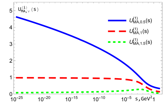
Figure 1: The results for $U^{(1)}_{\rm MA,\nu}(Q^{2})$ with $\nu=0.5,1,1.5$ in logarithmic scale.

For the cases $\nu=0.5,1,1.5$, $U^{(1)}_{{\rm MA},\nu}(Q^{2})$ is shown in Fig. 3. Strictly speaking, the value of the parameter $\Lambda$ is obtained by fitting experimental data. To obtain its values (one of the two MA couplants $A_{\rm MA}(Q^{2})$ and $U_{\rm MA}(s)$ can be fitted as they are very close to each other, as will be shown on Figs. 7 and 8 below) within the framework of analytical QCD, it is necessary to fit experimental data for various processes by using, for instance, formulas obtained in this paper that simplify the form of higher-order terms. This, however, requires additional special research. In this article we use the values $\Lambda_{f=3}$ and $\Lambda_{f=5}$ (see Eq. (10)) obtained in the framework of a conventional perturbative QCD since PT and FAPT couplants must coincide in the limit of large $Q^{2}$ and this requirement is fulfilled. It is clearly seen that at low $Q^{2}$ $U^{(1)}_{{\rm MA},\nu}(Q^{2})$ agrees with its asymptotic values:

$$U^{(1)}_{{\rm MA},\nu}(Q^{2}=0)=\left\{\begin{array}[]{c}0~{}~{}\mbox{when}~{}~{}\nu>1,\\ 1~{}~{}\mbox{when}~{}~{}\nu=1,\\ \infty~{}~{}\mbox{when}~{}~{}\nu<1,\end{array}\right.$$ (16)

obtained in Ref. Ayala:2018ifo . The corresponding results in the Euclidean space for $A^{(1)}_{{\rm MA},\nu}(Q^{2})$ $\nu=0.5,1,1.5$ were numerically obtained and shown on Fig.1 in Kotikov:2022sos . They are very close to those shown above in Fig. 1. Moreover, the asymptotic values of $A^{(1)}_{{\rm MA},\nu}(Q^{2}=0)$ and $U^{(1)}_{{\rm MA},\nu}(s=0)$ are completely identical to each other.

III.2 Beyond LO

Hereafter we repeat for $U_{{\rm MA},\nu}(s)$ the procedure that was applied to $\tilde{a}_{\nu}^{(i)}(Q^{2})$. For this purpose, following to the representation (14) for the LO MA couplant in the Minkowski space, we consider its derivatives

$$\tilde{U}_{{\rm MA},n+1}(s)=\frac{(-1)^{n}}{n!}\,\frac{d^{n}U_{\rm MA}(s)}{(dL_{s})^{n}}\,.$$ (17)

Using the results (12) for the usual couplant we have

$$\tilde{U}^{{\rm MA},(i+1)}_{\nu}({\rm s})=\tilde{U}^{(1)}_{{\rm MA},\nu}({\rm s})+\sum_{m=1}^{i}\,C_{m}^{\nu+m}\,\tilde{\delta}^{(m+1)}_{\nu}({\rm s}),~{}~{}$$

$$\tilde{\delta}^{(m+1)}_{\nu}({\rm s})=\hat{R}_{m}\,\tilde{U}^{(1)}_{{\rm MA},\nu+m}({\rm s}),$$ (18)

where $\tilde{U}^{(1)}_{{\rm MA},\nu}({\rm s})$ is given in Eq. (14).

This approach allows to express the high order corrections in explicit form

$$\tilde{\delta}^{(m+2)}_{\nu}({\rm s})=\frac{1}{(\nu+m)\pi(\pi^{2}+L_{s}^{2})^{(\nu+m)/2}}\Bigl{\{}\overline{\delta}^{(m+2)}_{\nu+m-1}({\rm s})\sin\bigl{(}(\nu+m)g\bigr{)}+\hat{\delta}^{(m+2)}_{\nu+m-1}({\rm s})g\cos\bigl{(}(\nu+m)g\bigr{)}\Bigr{\}},$$ (19)

where $\overline{\delta}^{(m+2)}_{\nu}({\rm s})$ and $\hat{\delta}^{(m+2)}_{\nu}({\rm s})$ are

$$\overline{\delta}^{(2)}_{\nu}({\rm s})=b_{1}\,\Bigl{[}\hat{Z}_{1}(\nu)-G\Bigr{]},~{}~{}\hat{\delta}^{(2)}_{\nu}({\rm s})=b_{1}\,,$$

$$\overline{\delta}^{(3)}_{\nu}({\rm s})=b_{2}+b_{1}^{2}\,\Bigl{[}\hat{Z}_{2}(\nu)-2G\hat{Z}_{1}(\nu)+G^{2}-g^{2}\Bigr{]},~{}~{}\hat{\delta}^{(3)}_{\nu}({\rm s})=2b_{1}^{2}\,\Bigl{[}\hat{Z}_{1}(\nu)-G\Bigr{]}\,,$$

$$\overline{\delta}^{(4)}_{\nu}({\rm s})=\frac{b_{3}}{2}+3b_{1}b_{2}\,\Bigl{[}Z_{1}(\nu)-\frac{11}{6}-G\Bigl{]}$$

$$+b_{1}^{3}\Bigl{[}\hat{Z}_{3}(\nu)-3G\hat{Z}_{2}(\nu)+3(G^{2}-g^{2})\hat{Z}_{1}(\nu)-G(G^{2}-3g^{2})\Bigr{]}\,,~{}~{}$$

$$\hat{\delta}^{(4)}_{\nu}({\rm s})=3b_{1}b_{2}+b_{1}^{3}\Bigl{[}3\hat{Z}_{2}(\nu)-6G\hat{Z}_{1}(\nu)+(3G^{2}-g^{2})\Bigr{]},$$

$$\overline{\delta}^{(5)}_{\nu}({\rm s})=\frac{1}{3}\Bigl{(}b_{4}+5b_{2}^{2}\Bigr{)}+2b_{1}b_{3}\Bigl{[}Z_{1}(\nu)-\frac{13}{6}-G\Bigl{]}$$

$$+6b_{1}^{2}b_{2}\Bigl{[}Z_{2}(\nu)-\frac{11}{3}Z_{1}(\nu)+\frac{38}{9}-2G\Bigl{(}Z_{1}(\nu)-\frac{11}{6}\Bigr{)}+G^{2}-g^{2}\Bigl{]}$$

$$+b_{1}^{4}\Biggl{[}\hat{Z}_{4}(\nu)-4G\hat{Z}_{3}(\nu)+6(G^{2}-g^{2})\hat{Z}_{2}(\nu)-4G(G^{2}-3g^{2})\hat{Z}_{1}(\nu)+G^{4}-6G^{2}g^{2}+g^{4}\Biggr{]},$$

$$\hat{\delta}^{(5)}_{\nu}({\rm s})=2b_{1}b_{3}+12b_{1}^{2}b_{2}\Bigl{[}Z_{1}(\nu)-\frac{11}{6}-G\Bigl{]}$$

$$+4b_{1}^{4}\Bigl{[}\hat{Z}_{3}(\nu)-3G\hat{Z}_{2}(\nu)+(3G^{2}-g^{2})\hat{Z}_{1}(\nu)-G(G^{2}-g^{2})\Bigr{]}$$ (20)

and

$$G({\rm s})=\frac{1}{2}\,\ln\left(\pi^{2}+L_{s}^{2}\right).$$ (21)

III.3 The case $\nu=1$

For the case $\nu=1$ we get

$$\tilde{U}^{(i+1)}_{{\rm MA},\nu=1}({\rm s})=\tilde{U}^{(1)}_{{\rm MA},\nu=1}({\rm s})+\sum_{m=1}^{i}\,\tilde{\delta}^{(m+1)}_{\nu=1}({\rm s}),$$ (22)

where LO gives the famous Shirkov-Solovtsov result ShS ; Sh

$$U^{(1)}_{{\rm MA}}({\rm s})=\tilde{U}^{(1)}_{{\rm MA},\nu=1}({\rm s})=\frac{g(s)}{\pi}=\frac{1}{\pi}\arccos\left(\frac{L_{s}}{\sqrt{L_{s}^{2}+\pi^{2}}}\right)=\frac{1}{\pi}\left(\frac{\pi}{2}-\arctan\left(\frac{L_{s}}{\pi}\right)\right)$$ (23)

and the high order corrections sufficiently simplify

$$\tilde{\delta}^{(m+1)}_{\nu=1}({\rm s})=\frac{1}{m\pi(\pi^{2}+L_{s}^{2})^{m/2}}\Bigl{\{}\overline{\delta}^{(m+1)}_{m-1}({\rm s})\sin\bigl{(}mg\bigr{)}+\hat{\delta}^{(m+1)}_{m-1}({\rm s})g\cos\bigl{(}mg\bigr{)}\Bigr{\}},$$ (24)

where $\overline{\delta}^{(m+1)}_{m-1}({\rm s})$ and $\hat{\delta}^{(m+1)}_{m-1}({\rm s})$ can be obtained from the corresponding values in Eq. (20) with $\nu=1$. Using Eqs. (A1) and (A2) we get

$$\overline{\delta}^{(2)}_{0}({\rm s})=-b_{1}\,\Bigl{[}1+G\Bigr{]},~{}~{}\hat{\delta}^{(2)}_{0}({\rm s})=b_{1}\,,$$

$$\overline{\delta}^{(3)}_{1}({\rm s})=b_{2}+b_{1}^{2}\,\Bigl{[}G^{2}-g^{2}-1\Bigr{]},~{}~{}\hat{\delta}^{(3)}_{1}({\rm s})=-2G\,b_{1}^{2}\,,$$

$$\overline{\delta}^{(4)}_{2}({\rm s})=\frac{b_{3}}{2}-b_{1}b_{2}\,\Bigl{[}1+3G\Bigl{]}+\frac{b_{1}^{3}}{2}\Bigl{[}1+6G+3(G^{2}-g^{2})-2G(G^{2}-3g^{2})\Bigr{]}\,,~{}~{}$$

$$\hat{\delta}^{(4)}_{2}({\rm s})=3b_{1}b_{2}+b_{1}^{3}\Bigl{[}3G^{2}-g^{2}-3G-3\Bigr{]},$$

$$\overline{\delta}^{(5)}_{3}({\rm s})=\frac{1}{3}\Bigl{(}b_{4}+5b_{2}^{2}\Bigr{)}-\frac{2}{3}\,b_{1}b_{3}\Bigl{[}1+3G\Bigl{]}+3b_{1}^{2}b_{2}\Bigl{[}2G^{2}-2g^{2}-1\Bigl{]}$$

$$+b_{1}^{4}\Biggl{[}\frac{5}{3}+2G-4(G^{2}-g^{2})-\frac{10}{3}G(G^{2}-3g^{2})+G^{4}-6G^{2}g^{2}+g^{4}\Biggr{]},$$

$$\hat{\delta}^{(5)}_{3}({\rm s})=2b_{1}b_{3}-12Gb_{1}^{2}b_{2}+2b_{1}^{4}\Bigl{[}4G-1+\frac{5}{3}(3G^{2}-g^{2})-2G(G^{2}-g^{2})\Bigr{]}\,.$$ (25)

Another form of $\tilde{\delta}^{(i+1)}_{\nu=1}({\rm s})$ is given in Appendix A (see Eq. (A3)).

At the point $s=\Lambda^{2}$ the above results are simplified. They are

$$\tilde{U}^{(i+1)}_{{\rm MA},\nu=1}({\rm{s}=\Lambda^{2}})=\tilde{U}^{(1)}_{{\rm MA},\nu=1}({\rm{s}=\Lambda^{2}})+\sum_{m=1}^{i}\,\tilde{\delta}^{(m+1)}_{\nu=1}({\rm s}=\Lambda^{2}),$$ (26)

where LO gives

$$U^{(1)}_{{\rm MA},1}({\rm s}=\Lambda^{2})=\frac{1}{2}$$ (27)

and the high order corrections are

$$\tilde{\delta}^{(2m+1)}_{\nu=1}({\rm s}=\Lambda^{2})=\frac{(-1)^{m}}{4m(\pi^{2}+L_{s}^{2})^{m}}\hat{\delta}^{(2m+1)}_{2m-1}({\rm s}=\Lambda^{2}),~{}~{}$$

$$\tilde{\delta}^{(2m+2)}_{\nu=1}({\rm s})=\frac{(-1)^{m}}{(2m+1)\pi(\pi^{2}+L_{s}^{2})^{m+1/2}}\,\overline{\delta}^{(2m+2)}_{2m}({\rm s}=\Lambda^{2})$$ (28)

where $\overline{\delta}^{(2m+2)}_{2m}({\rm s}=\Lambda^{2})$ and $\hat{\delta}^{(2m+1)}_{2m-1}({\rm s}=\Lambda^{2})$ can be taken from Eq. (25) with the following replacement:

$$G(s=\Lambda^{2})=\ln(\pi),~{}~{}g(s=\Lambda^{2})=\frac{\pi}{2}\,.$$ (29)

III.4 Discussions

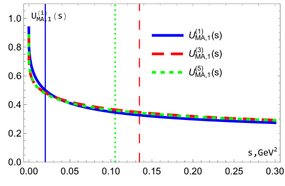
Figure 2: 1,3 and 5 orders of $U_{{\rm MA},\nu=1}^{(i)}$ .The vertical lines indicate $(\Lambda^{f=3}_{i-1})^{2}$

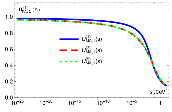
Figure 3: 1,3 and 5 orders of $U_{{\rm MA},\nu=1}^{(i)}$ with logarithmic scale of $s$

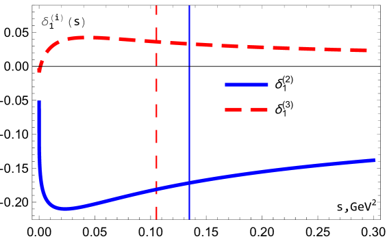
Figure 4: $\delta_{{\rm MA},\nu=1}^{(i)}$ with $i=2,3$.The vertical lines indicate $(\Lambda^{f=3}_{i-1})^{2}$

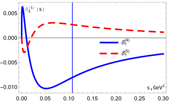
Figure 5: $\delta_{{\rm MA},\nu=1}^{(i)}$ with $i=4,5$. The vertical line indicates $(\Lambda^{f=3}_{3})^{2}=\Lambda^{f=3}_{4})^{2}$

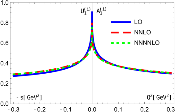
Figure 6: 1,3 and 5 orders of $U_{{\rm MA},\nu=1}^{(i)}$ and $A_{{\rm MA},\nu=1}^{(i)}$

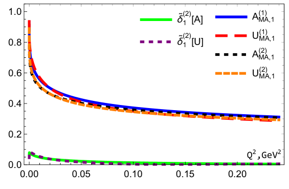
Figure 7: 1 and 2 orders of $U_{{\rm MA},\nu=1}^{(i)}$, $A_{{\rm MA},\nu=1}^{(i)}$ and $\delta_{{\rm MA},\nu=1}^{(2)}$ in Euclidean and Minkowki spaces.

This subsection provides graphical results of couplant construction. Figs. 2 and 3 show the results for $U^{(i)}_{\rm MA,\nu=1}(s)$ with $i=1,3,5$ in usual and logarithmic scales (the last one was chosen to stress the limit $U^{(i)}_{\rm MA,\nu=1}(s\to 0)\to 1$). From Figs. 4 and 5 we can see the differences between $U^{(i)}_{\rm MA,\nu=1}(Q^{2})$ with $i=1,..,5$, which are rather small and have nonzero values around the position $Q^{2}=\Lambda_{i}^{2}$. In Figs. 2, 4, 5 and 8 the values of $(\Lambda_{i}^{f=3})^{2}$ $(i=0,2,4)$ are shown by vertical lines with color matching in each order. Note that Fig.5 contains only one vertical line since $(\Lambda_{4}^{f=3})^{2}=(\Lambda_{5}^{f=3})^{2}$.

So, Figs. 2-5 point out that the difference between $U^{(i+1)}_{\rm MA,\nu=1}(s)$ and $U^{(i)}_{\rm MA,\nu=1}(s)$ is essentially less then the couplants themselves. From Figs. 3, 4 and 5 it is clear that for $s\to 0$ the asymptotic behavior of $U^{(1)}_{\rm MA,\nu=1}(s)$, $U^{(3)}_{\rm MA,\nu=1}(s)$ and $U^{(5)}_{\rm MA,\nu=1}(s)$ coincides (and is equal to behavior considered in (16)), i.e. the differences $\delta^{(i)}_{\rm MA,\nu=1}(s\to 0)$ are negligible. Also Figs. 4 and 5 show the differences $\delta^{(i+1)}_{\rm MA,\nu=1}(s)$ $(i\geq 2)$ essentially less then $\delta^{(2)}_{\rm MA,\nu=1}(s)$. We note that general form of the results is exactly the same as in the case of the MA couplants $A^{(i+1)}_{\rm MA,\nu,i}(Q^{2})$, which have been studied earlier in Kotikov:2022sos .

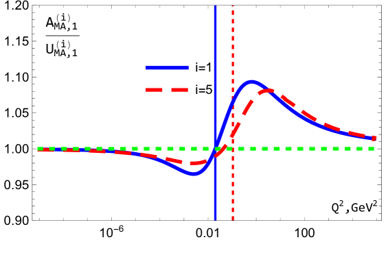
Figure 8: The relation $A^{(i)}_{\rm MA,\nu=1}/U^{(i)}_{\rm MA,\nu=1}$ for $i=1,5$. The vertical lines indicate $(\Lambda^{f=3}_{i-1})^{2}$.

Indeed, the similarity is shown in Figs. 6 and 7. In Fig. 6 the results for $U^{(i)}_{\rm MA,\nu=1}(s)$ and $A^{(i)}_{\rm MA,\nu=1}(Q^{2})$ ($i=1,3,5$) are shown in the so-called mirror form, which is in accordance with the similar one presented earlier in Bakulev:2006ex . Fig. 7 contains $U^{(1)}_{\rm MA,\nu=1}(s)$, $A^{(1)}_{\rm MA,\nu=1}(Q^{2})$, $U^{(2)}_{\rm MA,\nu=1}(s)$ and $A^{(2)}_{\rm MA,\nu=1}(Q^{2})$ which are very close to each others but have different limit values when $Q^{2}\to 0$. Moreover, the differences $\delta^{(2)}_{\rm MA,\nu=1}(Q^{2})$ in the cases $U^{(2)}_{\rm MA,\nu=1}(s)$ and $A^{(2)}_{\rm MA,\nu=1}(Q^{2})$ are almost the same although correction of the spacelike couplant decreases more rapidly. The direct relation between $A^{(i)}_{\rm MA,\nu=1}(Q^{2})$ and $U^{(i)}_{\rm MA,\nu=1}(Q^{2})$ gives an interesting picture (see Fig. 8). Obviously we have $\frac{A^{(i)}_{\rm MA,\nu=1}(Q^{2}=0)}{U^{(i)}_{\rm MA,\nu=1}(Q^{2}=0)}=1$ for any order and the second similar point

$$\frac{A^{(i)}_{\rm MA,\nu=1}(Q^{2}=(\Lambda^{f=3}_{i-1})^{2})}{U^{(i)}_{\rm MA,\nu=1}(Q^{2}=(\Lambda^{f=3}_{i-1})^{2})}=1$$ (30)

for $i=1$. Higher order corrections break the identity (30), shifting the second point from $(\Lambda^{f=3}_{i})^{2}$. As we can see in Fig. 8, the shift is quite small. As can be seen from Fig. 8, the ratio (30) asymptotically approaches 1 when Q² $\to\infty$.

Thus, we can conclude that contrary to the case of the usual couplant, the $1/L$-expansion of the MA couplant is very good approximation at any $Q^{2}(s)$ values. Moreover, the differences between $U^{(i+1)}_{\rm MA,\nu=1}(s)$ and $U^{(i)}_{\rm MA,\nu=1}(s)$ become smaller with the increase of order. So, the expansions of $U^{(i+1)}_{\rm MA,\nu=1}(s)$ $i\geq 1$ through the $U^{(1)}_{\rm MA,\nu=1}(s)$ done in Refs. BMS1 ; Bakulev:2006ex ; Bakulev:2010gm are very good approximations.

IV Integral representations for minimal analytic coupling

As it was abovementioned in Introduction, the MA couplants $A^{(1)}_{\rm MA,\nu}(Q^{2})$ and $U^{(1)}_{\rm MA,\nu}(s)$ are constructed as follows: the LO spectral function is taken directly from perturbation theory but the MA couplants $A^{(1)}_{\rm MA,\nu}(Q^{2})$ and $U^{(1)}_{\rm MA,\nu}(s)$ themselves were obtained using the correct integration contours. Thus, at LO, the MA couplants $A^{(1)}_{\rm MA,\nu}(Q^{2})$ and $U^{(1)}_{\rm MA,\nu}(s)$ obey Eqs. (5) and (7) presented in Introduction.

To check Eqs. (24) and (20) we compare them with an integral form

$$U^{(i)}_{1}({\rm s})=\frac{1}{\pi}\int\limits^{\infty}_{s}\frac{d\sigma}{\sigma}r^{(i)}_{{\rm pt}}(\sigma).$$ (31)

For LO, we can take the integral form from Bakulev:2006ex

$$U^{(1)}_{\nu}({\rm s})=\frac{1}{\pi}\int\limits^{\infty}_{s}\frac{d\sigma}{\sigma}r^{(1)}_{\nu}(\sigma),$$ (32)

where

$$r^{(1)}_{\nu}({\rm s})=\frac{\sin[\nu\,g(s)]}{\pi(\pi^{2}+L^{2}_{s})^{(\nu-1)/2}}=\nu\,U^{(1)}_{\nu+1}({\rm s})\,,$$ (33)

In (14) only the case $\nu\geq 0$ is considered, it means that the integral (32) converges to zero at the upper limit. We would like to note, that dispersion integral (31) does not converge for some $\nu$ and, in this case, we will introduce constant, which corresponds to the upper limit of the integral. In general situation, it is better to replace the integral (31) by the one

$$U^{(1)}_{\nu}({\rm s})=\frac{1}{\pi}\int\limits^{\infty}_{s}\frac{d\sigma}{\sigma}r^{(1)}_{\nu}(\sigma)-U^{(1)}_{\nu}(\infty),$$ (34)

where

$$U^{(1)}_{\nu}(\infty)=\left\{\begin{array}[]{c}0~{}~{}\mbox{when}~{}~{}\nu>0,\\ 1~{}~{}\mbox{when}~{}~{}\nu=0,\\ \infty~{}~{}\mbox{when}~{}~{}\nu<0.\end{array}\right.$$ (35)

We see that the expression (32) diverges for $\nu<0$ and requires additional constant for $\nu=0$. Therefore Eq. (14) is applicable only when $\nu>0$. Further in this paper we will only consider the region $\nu>0$.

Using our approach to obtain high-order terms from LO (32), we can extend the LO integral (32) to the one

$$\tilde{U}^{(i)}_{\nu}({\rm s})=\frac{1}{\pi}\int\limits^{\infty}_{s}\frac{d\sigma}{\sigma}r^{(i)}_{\nu}(\sigma),$$ (36)

where obviously

$$r^{(i)}_{\nu}({\rm s})=\nu\,\tilde{U}^{(i)}_{\nu+1}({\rm s})\,.$$ (37)

The spectral function $r^{(i)}_{1}({\rm s})$ has the form

$$r^{(i)}_{1}({\rm s})=r^{(1)}_{1}({\rm s})+\sum_{m=1}^{i}\,\delta^{(m+1)}_{1}({\rm s})\,$$ (38)

where

$$r^{(1)}_{1}({\rm s})=U^{(1)}_{2}({\rm s}),~{}~{}\delta^{(m+1)}_{1}({\rm s})=(m+1)\,\tilde{\delta}^{(m+1)}_{\nu=2}({\rm s}).$$ (39)

In the explicit form:

$$r^{(i)}_{1}({\rm s})=\frac{\sin(g)}{\pi(\pi^{2}+L_{s}^{2})^{1/2}}=\frac{1}{\pi^{2}+L_{s}^{2}},$$

$$\tilde{\delta}^{(m+1)}_{1}({\rm s})=\frac{1}{\pi(\pi^{2}+L_{s}^{2})^{(m+1)/2}}\Bigl{\{}\overline{\delta}^{(m+1)}_{m}({\rm s})\sin\bigl{(}(m+1)g\bigr{)}+\hat{\delta}^{(m+1)}_{m}({\rm s})g\cos\bigl{(}(m+1)g\bigr{)}\Bigr{\}},$$ (40)

where $\overline{\delta}^{(m+1)}_{m}({\rm s})$ and $\hat{\delta}^{(m+1)}_{m}({\rm s})$ can be obtained from the results in (20) with $\nu=2$. They are

$$\overline{\delta}^{(2)}_{1}({\rm s})=-G\,b_{1},~{}~{}\hat{\delta}^{(2)}_{1}({\rm s})=b_{1}\,,$$

$$\overline{\delta}^{(3)}_{2}({\rm s})=b_{2}+b_{1}^{2}\,\Bigl{[}G^{2}-g^{2}-G-1\Bigr{]},~{}~{}\hat{\delta}^{(3)}_{2}({\rm s})=b_{1}^{2}\,\Bigl{[}1-2G\Bigr{]}\,,$$

$$\overline{\delta}^{(4)}_{3}({\rm s})=\frac{b_{3}}{2}-3G\,b_{1}b_{2}+\frac{b_{1}^{3}}{2}\Bigl{[}4G-1+5(G^{2}-g^{2})-2G(G^{2}-3g^{2})\Bigr{]}\,,~{}~{}$$

$$\hat{\delta}^{(4)}_{3}({\rm s})=3b_{1}b_{2}+b_{1}^{3}\Bigl{[}3G^{2}-g^{2}-5G-2\Bigr{]},$$

$$\overline{\delta}^{(5)}_{4}({\rm s})=\frac{1}{3}\Bigl{(}b_{4}+5b_{2}^{2}\Bigr{)}-2\,b_{1}b_{3}\Bigl{[}\frac{1}{12}+G\Bigl{]}+3b_{1}^{2}b_{2}\Bigl{[}2G^{2}-2g^{2}-G-1\Bigl{]}$$

$$+b_{1}^{4}\Biggl{[}\frac{7}{6}+4G-\frac{3}{2}(G^{2}-g^{2})-\frac{13}{3}G(G^{2}-3g^{2})+G^{4}-6G^{2}g^{2}+g^{4}\Biggr{]},$$

$$\hat{\delta}^{(5)}_{4}({\rm s})=2b_{1}b_{3}+3b_{1}^{2}b_{2}\Bigl{[}1-4G\Bigr{]}+b_{1}^{4}\Bigl{[}3G-4+\frac{13}{3}(3G^{2}-g^{2})-4G(G^{2}-g^{2})\Bigr{]}\,.$$ (41)

Using the results (A1) and (A2) for $\cos(ng)$ and $\sin(ng)$ $(n\leq 4)$, we see that with the results NeSi ; Nesterenko:2017wpb (see also Section 6 in Kotikov:2022sos ) give more compact results for $r^{(i)}_{1}({\rm s})$. We think that Eqs. (40) and (41) give apparently very compact results for $r^{(i)}_{1}({\rm s})$.

Note that the results (36) for $\tilde{U}^{(i)}_{\nu}({\rm s})$ are exactly the same as the results in Eq. (18) done in the form of trigonometric factions. However the results (36) should be very handy in case of non-minimal versions of analytic couplants (see Refs. Cvetic:2006mk ; Cvetic:2006gc ; Cvetic:2010di ).

V $H\to b\overline{b}$ decay

In Ref. Kotikov:2022sos we used the polarized Bjorken sum rule Chen:2006tw as an example for the application of the MA couplant $A_{\rm MA}(Q^{2})$, which is a popular object of study in the framework of analytic QCD (see Pasechnik:2008th ; Ayala:2017uzx ; Ayala:2018ulm ; Kotikov:2012eq ). Here we consider the decay of the Higgs boson into a bottom-antibottom pair, which is also a popular application of the MA couplant $U_{\rm MA}(Q^{2})$ (see, e.g., Bakulev:2006ex and reviews in Ref. Bakulev:2008td ).

The Higgs-boson decay into a bottom-antibottom pair can be expressed in QCD by means of the correlator

$$\Pi(Q^{2})=(4\pi)^{2}i\int\,dxe^{iqx}<0|T[J_{b}^{S}(x)J_{b}^{S}(0)]0>$$ (42)

of two quark scalar (S) currents in terms of the discontinuity of its imaginary part, i.e., $R_{S}(s)={\bf Im}\Pi(-s-i\varepsilon)/(2\pi s)$, so that the width reads

$$\Gamma(H\to b\overline{b})=\frac{G_{F}}{4\sqrt{2}\pi}M_{H}m^{2}_{b}(M^{2}_{H})R_{s}(s=M^{2}_{H})\,.$$ (43)

Direct multi-loop calculations were performed in the Euclidean (spacelike) domain for the corresponding Adler function $D_{S}$ (see Refs. Broadhurst:2000yc ; Chetyrkin:1996sr ; Baikov:2005rw ; Chetyrkin:1997wm ). Hence, we write ($D_{s}\to\tilde{D}_{s}$ and $R_{s}\to\tilde{R}_{s}$ because the additional factor $m_{b}^{2}$)

$$\tilde{D}(Q^{2})=3m_{b}^{2}(Q^{2})\Bigl{[}1+\sum_{n\geq 1}d_{n}\,a^{n}_{s}(Q^{2})\Bigr{]},$$ (44)

where for $f=5$ the coefficients $d_{n}$ are

$$d_{1}=2.96,~{}~{}d_{2}=11.44,~{}~{}d_{2}=50.17,~{}~{}d_{4}=260.24,~{}~{}$$ (45)

Taking the imagine part, one has

$$\tilde{R}_{s}(s)=3m_{b}^{2}(s)\Bigl{[}1+\sum_{n\geq 1}r_{n}\,a^{n}(s)\Bigr{]},$$ (46)

and for $f=5$ Baikov:2005rw ; Kataev:1993be

$$r_{1}=2.96,~{}~{}r_{2}=7.93,~{}~{}r_{3}=5.93,~{}~{}r_{4}=-61.84,~{}~{}$$ (47)

Here $\overline{m}_{b}^{2}(Q^{2})$ has the form (see Appendix B):

$$\overline{m}_{b}^{2}(Q^{2})=\hat{m}_{b}^{2}a_{s}^{d}(Q^{2})\,\left[1+\sum_{k=1}^{k=4}\,\overline{e}_{k}\,a_{s}^{k}(Q^{2})\right]\,,$$ (48)

where

$$\overline{e}_{k}=\frac{\tilde{e}_{k}}{k(\beta_{0})^{k}}$$ (49)

and $\tilde{e}_{k}$ are done in Eq. (B8). For $f=5$ we have

$$\overline{e}_{1}=1.23,~{}~{}\overline{e}_{2}=1.20,~{}~{}\overline{e}_{3}=0.55,~{}~{}\overline{e}_{4}=0.54\,.~{}~{}$$ (50)

The normalization constant $\hat{m}_{b}$ cab be obtained as (see, e.g., Bakulev:2008td )

$$\hat{m}_{b}=\overline{m}_{b}(Q^{2}=m_{b}^{2})a_{s}^{-d/2}(m_{b}^{2})\,{\left[1+\sum_{k=1}^{k=4}\,\overline{e}_{k}\,a_{s}^{k}(Q^{2})\right]}^{-1/2}=10.814~{}\mbox{GeV}^{2}\,,$$ (51)

since $\overline{m}_{b}(Q^{2}=m_{b}^{2})=m_{b}=4.18$ GeV.

So, we have

$$\tilde{R}_{s}(s)=\tilde{R}^{(m=5)}_{s}(s),~{}~{}\tilde{R}^{(m+1)}_{s}(s)=3\hat{m}_{b}^{2}\,a_{s}^{d}(s)\,\left[1+\sum_{k=0}^{m}\overline{r}_{k}a_{s}^{k}(s))\right],$$ (52)

where

$$\overline{r}_{k}=r_{k}+\overline{e}_{k}+\sum_{l=1}^{k-1}r_{l}\,\overline{e}_{k-l}\,.$$ (53)

For $f=5$ we have

$$\overline{r}_{1}=4.18,~{}~{}\overline{r}_{2}=12.76,~{}~{}\overline{r}_{3}=19.76,~{}~{}\overline{r}_{4}=-42.25\,.~{}~{}$$ (54)

We can express all results through derivatives $\tilde{a}_{d+k}$ (see Appendix B):

$$\tilde{R}_{s}(s)=\tilde{R}^{(m=5)}_{s}(s),~{}~{}\tilde{R}^{(m+1)}_{s}(s)=3\hat{m}_{b}^{2}\left[\tilde{a}_{d}+\sum_{k=0}^{m}\tilde{r}_{k}\tilde{a}_{d+k}\right],$$ (55)

where

$$\tilde{r}_{k}=\overline{r}_{k}+\tilde{k}_{k}(d)+\sum_{l=1}^{k-1}\overline{r}_{l}\,\tilde{k}_{k-l}(d+l)\,,$$ (56)

where $\tilde{k}_{i}(\nu)$ are given in Appendix C.

For $d=24/23$ and $f=5$, we have

$$\tilde{r}_{1}=4.17,~{}~{}\tilde{r}_{2}=9.86,~{}~{}\tilde{r}_{3}=1.29,~{}~{}\tilde{r}_{4}=-71.21\,.$$ (57)

Performing the same analysis for the Adler function we have

$$\tilde{D}_{s}=\tilde{D}^{(m=5)}_{s},~{}~{}\tilde{D}^{(m+1)}_{s}=3\hat{m}_{b}^{2}a_{s}^{d}(Q^{2})\,\left[1+\sum_{k=0}^{m}\overline{d}_{k}a_{s}^{k}(Q^{2}))\right],$$ (58)

where

$$\overline{d}_{k}=r_{k}+\overline{e}_{k}+\sum_{l=1}^{k-1}d_{l}\,\overline{e}_{k-l}\,.$$ (59)

For $f=5$ we have

$$\overline{d}_{1}=4.18,~{}~{}\overline{d}_{2}=16.27,~{}~{}\overline{d}_{3}=68.30,~{}~{}\overline{r}_{4}=337.66\,.~{}~{}$$ (60)

We express all results through derivatives $\tilde{a}_{d+k}$:

$$\tilde{D}_{s}=\tilde{D}^{(m=5)}_{s},~{}~{}\tilde{D}^{(m+1)}_{s}=3\hat{m}_{b}^{2}\left[\tilde{a}_{d}(Q^{2})+\sum_{k=0}^{m}\tilde{d}_{k}\tilde{a}_{d+k}(Q^{2})\right],$$ (61)

where

$$\tilde{d}_{k}=\overline{d}_{k}+\tilde{k}_{k}(d)+\sum_{l=1}^{k-1}\overline{d}_{l}\,\tilde{k}_{k-l}(d+l)\,.$$ (62)

For $f=5$ and $d=24/23$, we have

$$\tilde{d}_{1}=4.17,~{}~{}\tilde{d}_{2}=13.37,~{}~{}\tilde{d}_{3}=43.90,~{}~{}\tilde{d}_{4}=178.18\,.~{}~{}$$ (63)

As it was discussed earlier in Bakulev:2006ex in FAPT there are the following representation for $\tilde{R}_{s}$

$$\tilde{R}_{s}(s)=\tilde{R}^{(m=5)}_{s}(s),~{}~{}\tilde{R}^{(m+1)}_{s}(s)=3\hat{m}_{b}^{2}\left[\tilde{U}^{(m+1)}_{d}({\rm s})+\sum_{k=0}^{m}\tilde{d}_{k}\,\tilde{U}^{(m+1)}_{d+k}(s)\right],$$ (64)

The results for $\tilde{R}^{(m+1)}_{s}(s)$ are shown in Fig. 9. We see that the FAPT results (64) are lower than those (55) based on the conventional PT. This is in full agreement with arguments given in Bakulev:2008td . But the difference becomes less notable as the PT order increases. Indeed, for N³LO the difference is very small, which proves the assumption about the possibility of using $\tilde{R}^{(m+1)}_{s}(s)$ expression for $\tilde{D}^{(m+1)}_{s}(Q^{2})$ with $A^{(i)}_{\rm MA}(Q^{2})\to U^{(i)}_{\rm MA}(s)$, which was done in Ref. Bakulev:2006ex .

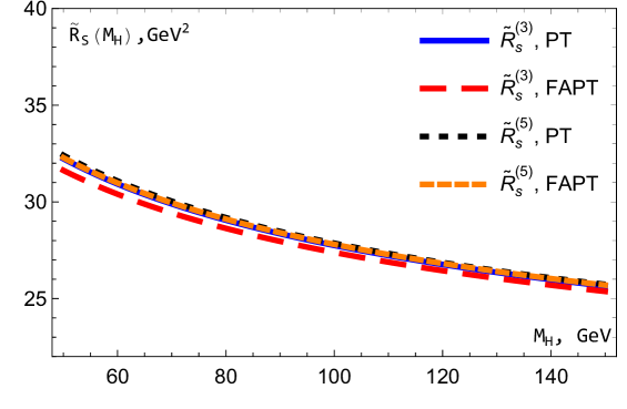
Figure 9: The results for $\tilde{R}^{(m+1)}_{s}(s)$ with $m=2$ and 4 in the framework of the usual PT and FAPT.

The results for $\Gamma^{(m)}(H\to b\overline{b})$ in the N^mLO approximation using $\tilde{R}^{(m+1)}_{s}(s)$ from Eqs. (52) and (55) are exactly same and have the following form:

$$\Gamma^{(0)}=1.76~{}\mbox{MeV},~{}\Gamma^{(1)}~{}=2.27~{}\mbox{MeV},~{}~{}\Gamma^{(2)}=2.37~{}\mbox{MeV},~{}~{}$$

$$\Gamma^{(3)}=2.38~{}\mbox{MeV},~{}~{}\Gamma^{(4)}=2.38~{}\mbox{MeV}\,.$$ (65)

The corresponding results for $\Gamma^{(m)}(H\to b\overline{b})$ with $\tilde{R}^{(m+1)}_{s}(s)$ form Eq. (64) are very similar to ones in (65). They are:

$$\Gamma^{(0)}=1.74~{}\mbox{MeV},~{}\Gamma^{(1)}~{}=2.23~{}\mbox{MeV},~{}~{}\Gamma^{(2)}=2.34~{}\mbox{MeV},~{}~{}$$

$$\Gamma^{(3)}=2.37~{}\mbox{MeV},~{}~{}\Gamma^{(4)}=2.38~{}\mbox{MeV}\,.$$ (66)

So, we see a good agreement between the results obtained in FAPT and in the framework of the usual PT.

It is clearly seen that the results of FAPT are very also close to the results Wang:2013bla obtained in the framework of the now very popular Principle of Maximum Conformality Brodsky:2011ta (for the recent review, see Shen:2022nyr ). Indeed, our results are within the band obtained by varying the renormalization scale.

The Standard Model expectation is LHCHiggsCrossSectionWorkingGroup:2016ypw

$$\Gamma^{SM}_{H\to b\overline{b}}(M_{H}=125.1\mbox{GeV})=2.38\mbox{MeV}\,.$$ (67)

The ratios of the measured events yield to the Standard Model expectations are $1.01\pm 0.12(\mbox{stat}.)+0.16-0.15(\mbox{syst}.)$ ATLAS:2018kot in ATLAS Collaboration and $1.04\pm 0.14(\mbox{stat}.)\pm 0.14(\mbox{syst}.)$ CMS:2018nsn in SMC Collaboration (see also Tsukerman:2020qwz ).

Thus, our results obtained in both approaches, in the standard perturbation theory and in analytical QCD, are in good agreement both with the Standard Model expectations LHCHiggsCrossSectionWorkingGroup:2016ypw and with the experimental data ATLAS:2018kot ; CMS:2018nsn .

VI Conclusions

In this paper we have used $1/L$-expansions of the $\nu$-derivatives of the strong couplant $a_{s}$ expressed Kotikov:2022sos as combinations of operators $\hat{R}_{m}$ (13) applied to the LO couplant $a_{s}^{(1)}$. Applying the same operators to the $\nu$-derivatives of the LO MA couplant $U_{\rm MA}^{(1)}$, we obtained two different representations (see Eqs. (24) and (36)) for the $\nu$-derivatives of the MA couplants, i.e. $\tilde{U}_{\rm MA,\nu}^{(i)}$ introduced for timelike processes, in each $i$-order of perturbation theory: one form contains a combinations of trigonometric functions, and the other is based on dispersion integrals containing the $i$-order spectral function. All results are presented up to the 5th order of perturbation theory, where the corresponding coefficients of the QCD $\beta$-function are well known (see Baikov:2016tgj ; Herzog:2017ohr ).

As in the case of $\tilde{A}_{\rm MA,\nu}^{(i)}$ Kotikov:2022sos applied in the Euclidean space, high-order corrections for $\tilde{U}_{\rm MA,\nu}^{(i)}$ are negligible in the $s\to 0$ and $s\to\infty$ limits and are nonzero in the vicinity of the point $s=\Lambda^{2}$. Thus, in fact, there are actually only small corrections to the LO MA couplant $U_{\rm MA,\nu}^{(1)}(s)$. In particular, this proves the possibility of expansions of high-order couplants $U_{\rm MA,\nu}^{(i)}(s)$ via the LO couplants $U_{\rm MA,\nu}^{(1)}(s)$, which was done in Ref. Bakulev:2010gm .

As an example, we examined the Higgs boson decay into a $b\overline{b}$ pair and obtained results are in good agreement with the Standard Model expectations LHCHiggsCrossSectionWorkingGroup:2016ypw and with the experimental data ATLAS:2018kot ; CMS:2018nsn . Moreover, our results also in good agreement with studies based on the Principle Maximum Conformality Brodsky:2011ta .

As a next step, we plan to include $1/L$-expansions for other MA couplants (see Refs. Bakulev:2006ex ; Bakulev:2010gm ; Ayala:2018ifo ; Mikhailov:2021znq ), as well as for non-minimal analytic couplants (following Refs. Cvetic:2006mk ; Cvetic:2006gc ; Cvetic:2010di ; CPCCAGC ; 3dAQCD ). In the case of non-minimal analytic couplants, one can use the integral representations (32) and (36) with non-perturbative spectral functions.

VII Acknowledgments

We are grateful to Andrey Kataev for discussions. We also thank the anonymous Referee, whose comments greatly improved the quality of the paper. This work was supported in part by the Foundation for the Advancement of Theoretical Physics and Mathematics “BASIS”.

Appendix A Another form for $U^{(i+1)}_{1}({\rm s})$

Using the results in Eq. (15) and transformation rules for $\sin(ng)$ and $\cos(ng)$, we have

$$\sin(ng)=\frac{S(ng)}{(\pi^{2}+L_{s}^{2})^{n/2}},~{}~{}\cos(ng)=\frac{C(ng)}{(\pi^{2}+L_{s}^{2})^{n/2}},$$ (A1)

where

$$S(g)=\pi,~{}~{}C(g)=L_{s},~{}~{}S(2g)=2\pi L_{s},~{}~{}C(2g)=L_{s}^{2}-\pi^{2},~{}~{}S(3g)=\pi(3L_{s}^{2}-\pi^{2}),~{}$$

$$~{}C(3g)=L_{s}(L_{s}^{2}-3\pi^{2}),~{}~{}S(4g)=4\pi L_{s}(L_{s}^{2}-\pi^{2}),~{}~{}C(4g)=L_{s}^{4}-6\pi^{2}L_{s}^{2}+\pi^{4},~{}$$

$$S(5g)=\pi(5L_{s}^{4}-10\pi^{2}L_{s}^{2}+\pi^{4}),~{}~{}C(5g)=L_{s}(L_{s}^{4}-10\pi^{2}L_{s}^{2}+5\pi^{4})\,.$$ (A2)

Using Eqs. (A1), (A2) and (25), the results for $\tilde{\delta}^{(m+1)}_{\nu=1}({\rm s})$ in (24) can be rewritten in the following form

$$\tilde{\delta}^{(2)}_{\nu=1}({\rm s})=\frac{b_{1}}{(\pi^{2}+L_{s}^{2})}\Bigl{(}\frac{g}{\pi}L_{s}-\bigl{(}1+G\bigr{)}\Bigr{)},$$

$$\tilde{\delta}^{(3)}_{\nu=1}({\rm s})=\frac{1}{(\pi^{2}+L_{s}^{2})^{2}}\Bigl{[}b_{2}L_{s}-b_{1}^{2}\Bigl{(}\frac{gG}{\pi}(L_{s}^{2}-\pi^{2})+L_{s}\bigl{(}1+g^{2}-G^{2}\bigr{)}\Bigr{)}\Bigr{]},$$

$$\tilde{\delta}^{(4)}_{\nu=1}({\rm s})=\frac{1}{(\pi^{2}+L_{s}^{2})^{3}}\Bigl{\{}b_{1}b_{2}\Bigl{(}\frac{gL_{s}}{\pi}(L^{2}_{s}-3\pi^{2})-\Bigl{(}L^{2}_{s}-\frac{1}{3}\pi^{2}\Bigr{)}\bigl{(}1+3G\bigr{)}\Bigr{)}$$

$$+\frac{b_{3}}{6}(3L^{2}_{s}-\pi^{2})+\frac{b_{1}^{3}}{6}\Bigl{(}(3L_{s}^{2}-\pi^{2})\Bigl{[}1+6G-3g^{2}+3G^{2}+6g^{2}G-2G^{3}\Bigr{]}$$

$$-\frac{2gL_{s}}{\pi}(L^{2}_{s}-3\pi^{2})\Bigl{[}3+3G+g^{2}-3G^{2}\Bigr{]}\Bigr{)}\Bigr{\}},$$

$$\tilde{\delta}^{(5)}_{\nu=1}({\rm s})=\frac{1}{(\pi^{2}+L_{s}^{2})^{4}}\Bigl{\{}3b_{1}^{2}b_{2}\Bigl{(}L_{s}(\pi^{2}-L_{s}^{2})\Bigl{[}1+2g^{2}-2G^{2}\Bigr{]}-\frac{gG}{\pi}(L_{s}^{4}-6L_{s}^{2}\pi^{2}+\pi^{4})\Bigr{)}$$

$$+2b_{1}b_{3}\Bigl{(}\frac{L_{s}}{3}(\pi^{2}-L_{s}^{2})\Bigl{[}1+3G\Bigr{]}+\frac{g}{4\pi}(L_{s}^{4}-6L_{s}^{2}\pi^{2}+\pi^{4})\Bigr{)}-\frac{5b_{2}^{2}+b_{4}}{3}L_{s}(\pi^{2}-L^{2}_{s})$$

$$+b_{1}^{4}\Bigl{(}L_{s}(\pi^{2}-L^{2}_{s})\Bigl{[}-\frac{5}{3}-2G-4g^{2}+4G^{2}-10g^{2}G+\frac{10}{3}G^{3}-g^{4}+6g^{2}G^{2}-G^{4}\Bigr{]}$$

$$+\frac{g}{2\pi}(L_{s}^{4}-6L_{s}^{2}\pi^{2}+\pi^{4})\Bigl{[}4G-1-\frac{5}{3}g^{2}+5G^{2}+2g^{2}G-2G^{3}\Bigr{]}\Bigr{)}\Bigr{\}},$$ (A3)

which is similar to the results for the spectral function $r^{(i)}_{1}({\rm s})$ done in ref.NeSi ; Nesterenko:2017wpb (see also Section 6 in Kotikov:2022sos ).

Appendix B $\overline{m}_{b}^{2}(Q^{2})$

Here we present evaluation of $\overline{m}_{b}^{2}(Q^{2})$, which has the form

$$\overline{m}_{b}^{2}(Q^{2})=\overline{m}_{b}^{2}(Q^{2})\,\exp\left[2\int^{\overline{a}_{s}(Q^{2})}_{\overline{a}_{s}(Q^{2}_{0})}\frac{\gamma_{m}(a)}{\beta_{(}a)}\right]\,,~{}~{}\overline{a}_{s}(Q^{2})=\frac{\alpha_{s}(Q^{2})}{4\pi}\,,$$ (B1)

where

$$\gamma_{m}(a)=-\sum_{k=0}\gamma_{k}a^{k+1}=-\gamma_{0}a\bigl{(}1+\sum_{k=1}\delta_{k}a^{k}\bigr{)},~{}~{}\delta_{k}=\frac{\gamma_{k}}{\gamma_{0}}\,,$$

$$\beta(a)=-\sum_{k=0}\beta_{k}a^{k+2}=-\beta_{0}a^{2}\bigl{(}1+\sum_{k=1}c_{k}a^{k}\bigr{)},~{}~{}c_{k}=\frac{\beta_{k}}{\beta_{0}}\,.$$ (B2)

Evaluating the integral in (B1) we have the following results (see, e.g., also Refs. Bakulev:2006ex ; Chetyrkin:1997dh )

$$\overline{m}_{b}^{2}(Q^{2})=\overline{m}_{b}^{2}(Q^{2})\,\frac{\overline{a}_{s}^{d}(Q^{2})}{\overline{a}_{s}^{d}(Q_{0}^{2})}\,\frac{T(\overline{a}_{s}(Q^{2}))}{T(\overline{a}_{s}(Q^{2}_{0}))}\,,$$ (B3)

where

$$d=\frac{2\gamma_{0}}{\beta_{0}},~{}~{}T(\overline{a}_{s})=\exp[\sum_{k=1}^{k=4}\frac{e_{k}}{k}\,\overline{a}_{s}^{k}]$$ (B4)

and

$$e_{1}=d\Delta_{1},~{}~{}e_{2}=d(\Delta_{2}-c_{1}\Delta_{1}),~{}~{}e_{3}=d(\Delta_{3}-c_{1}\Delta_{2}-\tilde{c}_{2}\Delta_{1}),$$

$$e_{4}=d(\Delta_{4}-c_{1}\Delta_{3}-\tilde{c}_{2}\Delta_{2}-\tilde{c}_{3}\Delta_{1})\,,$$ (B5)

with

$$\Delta_{i}=\delta_{i}-c_{i},~{}~{}\tilde{c}_{2}=c_{2}-c_{1}^{2},~{}~{}\tilde{c}_{3}=c_{3}-2c_{1}c_{2}+c_{1}^{3}$$ (B6)

The result for $T(\overline{a}_{s})$ can be rewritten as

$$T(\overline{a}_{s})=1+\sum_{k=1}^{k=4}\,\frac{\tilde{e}_{k}}{k}\,\overline{a}_{s}^{k}\,,$$ (B7)

where

$$\tilde{e}_{1}=e_{1},~{}~{}\tilde{e}_{2}=e_{2}+e_{1}^{2},~{}~{}\tilde{e}_{3}=e_{3}+\frac{3}{2}e_{1}e_{2}+\frac{1}{2}e_{1}^{3},$$

$$\tilde{e}_{3}=e_{4}+e_{2}^{2}+\frac{4}{3}e_{1}e_{3}+\frac{1}{2}e_{1}^{3}+e^{2}_{1}e_{2}+\frac{1}{6}e_{1}^{4},$$ (B8)

Appendix C Relations between $a_{s}^{\nu}$ and $\tilde{a}_{\nu}$

Considering Ref. GCAK we have

$$a_{s}^{\nu}=\tilde{a}_{\nu}+\sum_{m\geq 1}\,\tilde{k}_{m}(\nu)\,\tilde{a}_{\nu+m}\,,$$ (C1)

where

$$\tilde{k}_{1}(\nu)=-\nu b_{1}\tilde{B}_{1}(\nu),$$

$$\tilde{k}_{2}(\nu)=\nu(\nu+1)\left(-b_{2}\tilde{B}_{2}(\nu)+\frac{b_{1}^{2}}{2}\tilde{B}_{1,1}(\nu)\right),$$

$$\tilde{k}_{3}(\nu)=\frac{\nu(\nu+1)(\nu+2)}{2}\left(-b_{3}\tilde{B}_{3}(\nu)+b_{1}b_{2}\tilde{B}_{1,2}(\nu)-\frac{b_{1}^{3}}{3}\tilde{B}_{1,1,1}(\nu)\right),$$

$$\tilde{k}_{4}(\nu)=\frac{\nu(\nu+1)(\nu+2)(\nu+3)}{6}\Biggl{(}-b_{4}\tilde{B}_{4}(\nu)+b_{2}^{2}\tilde{B}_{2,2}(\nu)+\frac{b_{1}b_{3}}{2}\tilde{B}_{1,3}(\nu)$$

$$-\frac{b_{1}^{2}b_{2}}{2}\tilde{B}_{1,1,2}(\nu)+\frac{b_{1}^{4}}{4}\tilde{B}_{1,1,1,1}(\nu)\Biggr{)},$$ (C2)

where

$$\tilde{B}_{1}(\nu)=\tilde{Z}_{1}(\nu)-1,~{}~{}\tilde{B}_{2}(\nu)=\frac{\nu-1}{2(\nu+1)},~{}~{}\tilde{B}_{1,1}(\nu)=\tilde{Z}_{2}(\nu)-2\tilde{Z}_{1}(\nu+1)+1,$$

$$\tilde{B}_{3}(\nu)=\frac{1}{6}-\frac{1}{(\nu+1)(\nu+2)},~{}~{}\tilde{B}_{1,2}(\nu)=\frac{\nu-1}{6(\nu+1)}\,\Bigl{(}6\tilde{Z}_{1}(\nu+1)-1+\frac{4}{\nu+2}\Bigr{)},$$

$$\tilde{B}_{1,1,1}(\nu)=\tilde{Z}_{3}(\nu)-3\tilde{Z}_{2}(\nu+1)+3\tilde{Z}_{1}(\nu+2)-1,$$

$$\tilde{B}_{4}(\nu)=\frac{1}{12}-\frac{2}{(\nu+1)(\nu+2)(\nu+3)},~{}~{}\tilde{B}_{2,2}(\nu)=\frac{13}{12}-\frac{1}{\nu+1}-\frac{1}{\nu+2}-\frac{1}{\nu+3},$$

$$\tilde{B}_{1,3}(\nu)=\left(1-\frac{6}{(\nu+1)(\nu+2)}\right)\tilde{Z}_{1}(\nu+3)+\frac{1}{6}+\frac{4}{\nu+1}-\frac{5}{\nu+2}-\frac{2}{\nu+3},$$

$$\tilde{B}_{1,1,2}(\nu)=\frac{3(\nu-1)}{2(\nu+1)}\,\tilde{Z}_{2}(\nu+2)-\left(1-\frac{6}{(\nu+1)(\nu+2)}\right)\tilde{Z}_{1}(\nu+3)$$

$$+\frac{8}{3}-\frac{2}{\nu+1}+\frac{1}{\nu+2}-\frac{8}{\nu+3},$$

$$\tilde{B}_{1,1,1,1}(\nu)=\tilde{Z}_{4}(\nu)-4\tilde{Z}_{3}(\nu+1)+6\tilde{Z}_{2}(\nu+2)-4\tilde{Z}_{1}(\nu+3)+1$$ (C3)

and

$$\tilde{Z}_{1}(\nu)=S_{1}(\nu),~{}~{}\tilde{Z}_{2}(\nu)=S^{2}_{1}(\nu)+S_{2}(\nu),$$

$$\tilde{Z}_{3}(\nu)=S^{3}_{1}(\nu)+3S_{2}(\nu)S_{1}(\nu)+2S_{3}(\nu),$$

$$\tilde{Z}_{4}(\nu)=S^{4}_{1}(\nu)+6S_{2}(\nu)S^{2}_{1}(\nu)+3S_{2}^{2}(\nu)+8S_{3}(\nu)S_{1}(\nu)+6S_{4}(\nu)\,.$$ (C4)

For arbitrary $\nu$ values, $S_{i}(\nu)$ are expressed through Polygamma-functions as

$$S_{1}(\nu)=\Psi(\nu+1)-\Psi(1),~{}~{}\Psi(\nu)\equiv\frac{d}{d\nu}\ln\Gamma(\nu),~{}~{}\Psi^{(i)}(\nu)\equiv\frac{d^{i}}{(d\nu)^{i}}\Psi(\nu),$$

$$S_{i+1}(\nu)\equiv\frac{(-1)^{i}}{i!}\Bigl{(}\Psi^{(i)}(\nu+1)-\Psi^{(i)}(1)\Bigr{)}.$$ (C5)

In the case of integer $\nu=n$,

$$S_{i}(n)=\sum_{m=1}^{n}\,\frac{1}{m^{i}}\,.$$ (C6)

References

- (1) P. A. Baikov, K. G. Chetyrkin and J. H. Kühn, Phys. Rev. Lett. 118 (2017) no.8, 082002
- (2) F. Herzog, B. Ruijl, T. Ueda, J. A. M. Vermaseren and A. Vogt, JHEP 02 (2017), 090
- (3) T. Luthe, A. Maier, P. Marquard and Y. Schroder, JHEP 10 (2017), 166 K. G. Chetyrkin, G. Falcioni, F. Herzog and J. A. M. Vermaseren, JHEP 10 (2017), 179
- (4) D. V. Shirkov and I. L. Solovtsov, [arXiv:hep-ph/9604363 [hep-ph]]; Phys. Rev. Lett. 79 (1997), 1209-1212
- (5) K. A. Milton, I. L. Solovtsov and O. P. Solovtsova, Phys. Lett. B 415 (1997), 104-110
- (6) D. V. Shirkov, Theor. Math. Phys. 127 (2001), 409-423 Eur. Phys. J. C 22 (2001), 331-340
- (7) A. P. Bakulev, S. V. Mikhailov and N. G. Stefanis, Phys. Rev. D 72 (2005), 074014 [Erratum-ibid. D 72 (2005), 119908]
- (8) A. P. Bakulev, S. V. Mikhailov and N. G. Stefanis, Phys. Rev. D 75 (2007), 056005 [erratum: Phys. Rev. D 77 (2008), 079901]
- (9) A. P. Bakulev, S. V. Mikhailov and N. G. Stefanis, JHEP 06 (2010), 085
- (10) A. I. Karanikas and N. G. Stefanis, Phys. Lett. B 504 (2001), 225-234
- (11) A. P. Bakulev, Phys. Part. Nucl. 40 (2009), 715-756; N. G. Stefanis, Phys. Part. Nucl. 44 (2013), 494-509
- (12) G. Cvetic and C. Valenzuela, Braz. J. Phys. 38 (2008), 371-380
- (13) M. R. Pennington and G. G. Ross, Phys. Lett. B 102, 167-171 (1981); M. R. Pennington, R. G. Roberts and G. G. Ross, Nucl. Phys. B 242, 69-80 (1984); R. Marshall, Z. Phys. C 43, 595 (1989).
- (14) J. M. Cornwall, Phys. Rev. D 26 (1982), 1453
- (15) G. Parisi and R. Petronzio, Nucl. Phys. B 154 (1979), 427-440
- (16) N. V. Krasnikov and A. A. Pivovarov, Phys. Lett. B 116, 168-170 (1982); A. V. Radyushkin, JINR Rapid Commun. 78, 96-99 (1996) [arXiv:hep-ph/9907228 [hep-ph]].
- (17) A. P. Bakulev, A. V. Radyushkin and N. G. Stefanis, Phys. Rev. D 62, 113001 (2000); D. V. Shirkov, Theor. Math. Phys. 127, 409-423 (2001); Eur. Phys. J. C 22, 331-340 (2001) doi:10.1007/s100520100794 [arXiv:hep-ph/0107282 [hep-ph]].
- (18) A. V. Nesterenko, Int. J. Mod. Phys. A 18 (2003), 5475-5520
- (19) A. V. Nesterenko and J. Papavassiliou, Phys. Rev. D 71 (2005), 016009
- (20) A. V. Kotikov and I. A. Zemlyakov, J. Phys. G 50, no.1, 015001 (2023)
- (21) A. V. Kotikov and I. A. Zemlyakov, [arXiv:2207.01330 [hep-ph]]; [arXiv:2302.13769 [hep-ph]].
- (22) Particle Data Group collaboration, P.A. Zyla et al., Review of Particle Physics, PTEP 2020 (2020) 083C01.
- (23) K. G. Chetyrkin, J. H. Kuhn and C. Sturm, Nucl. Phys. B 744 (2006), 121-135
- (24) Y. Schroder and M. Steinhauser, JHEP 01 (2006), 051
- (25) B. A. Kniehl, A. V. Kotikov, A. I. Onishchenko and O. L. Veretin, Phys. Rev. Lett. 97 (2006), 042001
- (26) Y. Aoki et al., arXiv:2111.09849 [hep-lat].
- (27) D. d’Enterria, et al. [arXiv:2203.08271 [hep-ph]].
- (28) H. M. Chen, L. M. Liu, J. T. Wang, M. Waqas and G. X. Peng, Int. J. Mod. Phys. E 31 (2022) no.02, 2250016
- (29) G. Cvetic and C. Valenzuela, J. Phys. G 32 (2006), L27
- (30) G. Cvetic and C. Valenzuela, Phys. Rev. D 74 (2006), 114030 [erratum: Phys. Rev. D 84 (2011), 019902]
- (31) A. V. Kotikov and I. A. Zemlyakov, Pisma Zh. Eksp. Teor. Fiz. 115 (2022) no.10, 609
- (32) G. Cvetic, R. Kogerler and C. Valenzuela, Phys. Rev. D 82 (2010), 114004
- (33) G. Cvetič and A. V. Kotikov, J. Phys. G 39 (2012), 065005
- (34) A. V. Kotikov and L. N. Lipatov, Nucl. Phys. B 582 (2000), 19-43; Nucl. Phys. B 661 (2003), 19-61; A. V. Kotikov, L. N. Lipatov, A. I. Onishchenko and V. N. Velizhanin, Phys. Lett. B 595 (2004), 521-529; L. Bianchi, V. Forini and A. V. Kotikov, Phys. Lett. B 725 (2013), 394-401
- (35) A. P. Bakulev and V. L. Khandramai, Comput. Phys. Commun. 184 (2013) no.1, 183-193; V. Khandramai, J. Phys. Conf. Ser. 523 (2014), 012062 [arXiv:1310.5983 [hep-ph]]
- (36) C. Ayala, S. V. Mikhailov and N. G. Stefanis, Phys. Rev. D 98 (2018) no.9, 096017 [erratum: Phys. Rev. D 101 (2020) no.5, 059901]
- (37) A. V. Kotikov, V. G. Krivokhizhin and B. G. Shaikhatdenov, Phys. Atom. Nucl. 75 (2012), 507-524; A. V. Sidorov and O. P. Solovtsova, Mod. Phys. Lett. A 29 (2014) no.36, 1450194
- (38) V.G. Krivokhizhin and A.V. Kotikov, Yad.Fiz. 68 (2005) 1935; Phys.Part.Nucl. 40 (2009) 1059.
- (39) G. Parente, A.V. Kotikov and V.G. Krivokhizhin, Phys. Lett. B333 (1994) 190; A.V. Kotikov, G. Parente and J. Sanchez Guillen, Z. Phys. C58 (1993) 465; B. G. Shaikhatdenov et al., Phys. Rev. D 81 (2010), 034008
- (40) A. V. Kotikov, V. G. Krivokhizhin and B. G. Shaikhatdenov, JETP Lett. 101 (2015) 141-145; J. Phys. G 42 (2015) 095004; Phys. Atom. Nucl. 81 (2018) 244-252; JETP Lett. 115 (2022) no.8, 429-433
- (41) A.L. Kataev, A.V. Kotikov, G. Parente and A.V. Sidorov, Phys. Lett. B388 (1996) 179; Phys. Lett. B417 (1998) 374; A.V. Sidorov, Phys. Lett. B389 (1996) 379.
- (42) A.L. Kataev, G. Parente and A.V. Sidorov, Nucl. Phys. B573 (2000) 405; Phys. Part. Nucl. 34 (2003) 20.
- (43) G. Parisi and N. Sourlas, Nucl. Phys. B151 (1979) 421; V.G. Krivokhizhin et al., Z. Phys. C36 (1987) 51. Z. Phys. C48 (1990) 347.
- (44) T. J. Hou et al., Phys. Rev. D 103 (2021) no.1, 014013; S. Bailey et al., Eur. Phys. J. C 81 (2021) no.4, 341; R. D. Ball et al., Eur. Phys. J. C 81 (2021) no.10, 958; I. Abt et al. [H1 and ZEUS], Eur. Phys. J. C 82, no.3, 243 (2022); S. Alekhin, J. Blümlein, S. Moch and R. Placakyte, Phys. Rev. D 96 (2017) no.1, 014011, P. Jimenez-Delgado and E. Reya, Phys. Rev. D 89 (2014) no.7, 074049
- (45) V.N. Gribov and L.N. Lipatov, Sov. J. Nucl. Phys. 15 (1972) 438; L.N. Lipatov, Sov. J. Nucl. Phys. 20 (1975) 94; G. Altarelli and G. Parisi, Nucl. Phys. B126 (1977) 298; Yu.L. Dokshitzer, JETP 46 (1977) 641.
- (46) A. Buras, Rev. Mod. Phys. 52 (1980) 199.
- (47) D.I. Kazakov and A.V. Kotikov, Nucl.Phys. B307 (1988) 791; (E: 345, 299 (1990)); A.V. Kotikov and V.N. Velizhanin, hep-ph/0501274; A.V. Kotikov, Phys. Atom. Nucl.57 (1994) 133.
- (48) A. V. Nesterenko and C. Simolo, Comput. Phys. Commun. 181, 1769-1775 (2010)
- (49) A. V. Nesterenko, Eur. Phys. J. C 77, no.12, 844 (2017)
- (50) J. P. Chen, [arXiv:nucl-ex/0611024 [nucl-ex]]; J. P. Chen, A. Deur and Z. E. Meziani, Mod. Phys. Lett. A 20 (2005), 2745-2766
- (51) R. S. Pasechnik, D. V. Shirkov and O. V. Teryaev, Phys. Rev. D 78 (2008), 071902; R. S. Pasechnik, D. V. Shirkov, O. V. Teryaev, O. P. Solovtsova and V. L. Khandramai, Phys. Rev. D 81 (2010), 016010; V. L. Khandramai, R. S. Pasechnik, D. V. Shirkov, O. P. Solovtsova and O. V. Teryaev, Phys. Lett. B 706 (2012), 340-344
- (52) C. Ayala, G. Cvetic, A. V. Kotikov and B. G. Shaikhatdenov, Int. J. Mod. Phys. A 33 (2018) no.18n19, 1850112; J. Phys. Conf. Ser. 938 (2017) no.1, 012055
- (53) C. Ayala, G. Cvetič, A. V. Kotikov and B. G. Shaikhatdenov, Eur. Phys. J. C 78, no.12, 1002 (2018); J. Phys. Conf. Ser. 1435 (2020) no.1, 012016
- (54) A. V. Kotikov and B. G. Shaikhatdenov, Phys. Part. Nucl. 45 (2014), 26-29
- (55) D. J. Broadhurst, A. L. Kataev and C. J. Maxwell, Nucl. Phys. B 592, 247-293 (2001)
- (56) K. G. Chetyrkin, Phys. Lett. B 390, 309-317 (1997)
- (57) P. A. Baikov, K. G. Chetyrkin and J. H. Kuhn, Phys. Rev. Lett. 96, 012003 (2006); Acta Phys. Polon. B 48, 2135 (2017)
- (58) K. G. Chetyrkin, B. A. Kniehl and A. Sirlin, Phys. Lett. B 402, 359-366 (1997)
- (59) A. L. Kataev and V. T. Kim, Mod. Phys. Lett. A 9, 1309-1326 (1994); PoS ACAT08, 004 (2008)
- (60) S. Q. Wang, X. G. Wu, X. C. Zheng, J. M. Shen and Q. L. Zhang, Eur. Phys. J. C 74 (2014) no.4, 2825
- (61) S. J. Brodsky and X. G. Wu, Phys. Rev. D 85 (2012), 034038 [erratum: Phys. Rev. D 86 (2012), 079903]; Phys. Rev. Lett. 109 (2012), 042002; S. J. Brodsky and L. Di Giustino, Phys. Rev. D 86 (2012), 085026; M. Mojaza, S. J. Brodsky and X. G. Wu, Phys. Rev. Lett. 110 (2013), 192001; S. J. Brodsky, M. Mojaza and X. G. Wu, Phys. Rev. D 89 (2014), 014027
- (62) J. M. Shen, Z. J. Zhou, S. Q. Wang, J. Yan, Z. F. Wu, X. G. Wu and S. J. Brodsky, [arXiv:2209.03546 [hep-ph]]; J. Yan, Z. F. Wu, J. M. Shen and X. G. Wu, [arXiv:2209.13364 [hep-ph]].
- (63) D. de Florian et al. [LHC Higgs Cross Section Working Group], [arXiv:1610.07922 [hep-ph]].
- (64) M. Aaboud et al. [ATLAS], Phys. Lett. B 786 (2018), 59-86
- (65) A. M. Sirunyan et al. [CMS], Phys. Rev. Lett. 121 (2018) no.12, 121801
- (66) I. I. Tsukerman, Phys. Atom. Nucl. 83 (2020) no.2, 219-227
- (67) S. V. Mikhailov, A. V. Pimikov and N. G. Stefanis, Phys. Rev. D 103 (2021) no.9, 096003
- (68) C. Ayala and G. Cvetič, “anQCD: a Mathematica package for calculations in general analytic QCD models,” Comput. Phys. Commun. 190 (2015), 182-199; C. Ayala, C. Contreras and G. Cvetic, Phys. Rev. D 85 (2012), 114043
- (69) C. Ayala, G. Cvetič, R. Kögerler and I. Kondrashuk, J. Phys. G 45 (2018) no.3, 035001; G. Cvetič and R. Kögerler, J. Phys. G 48 (2021) no.5, 055008; C. Ayala, G. Cvetic and R. Kogerler, J. Phys. G 44 (2017) no.7, 075001
- (70) K. G. Chetyrkin, Phys. Lett. B 404, 161-165 (1997)