A Principal-Agent Framework
for Optimal Incentives in Renewable Investments

Abstract

We investigate the optimal regulation of energy production reflecting the long-term goals of the Paris Climate Agreement. We analyze the optimal regulatory incentives to foster the development of non-emissive electricity generation when the demand for power is served either by a monopoly or by two competing agents. The regulator wishes to encourage green investments to limit carbon emissions, while simultaneously reducing intermittency of the total energy production. We find that the regulation of a competitive market is more efficient than the one of the monopoly as measured with the certainty equivalent of the Principal’s value function. This higher efficiency is achieved thanks to a higher degree of freedom of the incentive mechanisms which involves cross-subsidies between firms. A numerical study quantifies the impact of the designed second-best contract in both market structures compared to the business-as-usual scenario.

In addition, we expand the monopolistic and competitive setup to a more general class of tractable Principal-Multi-Agent incentives problems when both the drift and the volatility of a multi-dimensional diffusion process can be controlled by the Agents. We follow the resolution methodology of Cvitanić et al.  (2018) in an extended linear quadratic setting with exponential utilities and a multi-dimensional state process of Ornstein-Uhlenbeck type. We provide closed-form expression of the second-best contracts. In particular, we show that they are in rebate form involving time-dependent prices of each state-variable.

JEL classification: C72, D86, Q28.

Keywords: Principal-Agent Problem, Contract Theory, Moral Hazard, Extended Linear Quadratic Cost, Optimal Regulation, Green Investments, Renewable Energy.

1 Introduction

This paper investigates Principal-Multi-Agent incentive problems inspired by the inescapable need for a suitable ‘green’ regulation reflecting long-term goals of the Paris Climate Agreement (see European Commission  (2016)). Investments in renewable energies such as wind and solar energy play an important role in the current climate debate. Due to their high fluctuations, however, conventional energy is still an attractive alternative for power producers even causing high carbon emissions. Regulation of the market in line with the green deal is necessary such that renewable energy generation is enforced to limit global warming.

However, an important feature of electricity generated by renewable energy, like solar and wind energy, is its intermittency. Their production depends on the realization of solar radiation and wind. Hence, the development of renewable energy increases the volatility of electricity production. Counter measures have to be taken into account to maintain the reliability of the power system. Thus, renewable energy provides both a positive externality thanks to the carbon emission they allow to avoid and a negative externality because of the indirect cost induced by their intermittency (see for an introduction to that economic literature Joskow  (2011), Borenstein  (2012), Hirth  (2013) and Gowrisankaran  (2016)). In this context, it makes perfect sense for the regulator to provide incentives to invest in renewables and also in counter measures to reduce the volatility they induce in the system (like storage or demand response enrollment programs).

Besides, the climate change and energy transition context, the present energy crisis that has taken over Europe in 2022 has triggered a series of public actions which trends toward an increase of the control of energy markets by the States. Indeed, the crisis raised voices on the necessity of a new market regulation (see European Commission  (2022)) while in France, the main electricity utility holding more than 75% of production capacity (in 2020) is becoming a fully national company.

This motivates our Principal-Agents approach to assess the optimal incentives mechanism to achieve an appropriate level of investment in non-emissive electricity production technology while maintaining smoothness of the energy production. Our approach builds on Cvitanić et al.  (2018) which itself is based on the work by Sannikov  (2008). In this work, Cvitanić et al.  (2018) provides a general solution for the design in continuous-time of an optimal contract with moral hazard when one is concerned with both drift and volatility control of the state variable. This result is of particular interest in a context where reducing the volatility of the intermittent renewable energy production is of the utmost importance. Their result was extended by Élie and Possamaï  (2019) to the case of Principal-Multi-Agent models but restricted to drift control only. This extension allows to deal with different market structures, like one regulated monopoly serving all the market or a competitive market served by several energy producers.

In this paper, we design an optimal contract, offered by the regulator (the Principal) encouraging energy producers (the Agents) to invest in renewable energy production capacity while stabilizing the energy production. In our model, agents can invest in two types of technology: intermittent renewable energy production capacity like wind farms and solar panels or conventional production technologies which are not intermittent but emissive like gas or coal fired plants. Agents receive a fixed proportional price for their production while facing linear quadratic investment costs with congestion term (product of both investment rates) captured by a single parameter $\varepsilon$. Further, they face a nonlinear volatility reduction cost function. Besides, installed capacities are prone to depreciation. The energy producers are incentivized to manage their production capacity level while controlling the energy production volatility. The regulator pays the producers for the energy they produce and bears three externalities. First, the conventional technology emits carbon emissions with constant unit value ($k_{1}$ in €/MWh), second, the renewable technology provides a positive social value of avoided emissions with a constant unit value ($k_{2}$ in €/MWh), and third, the renewable energy induces costly quadratic variation ($h$ in €/MWh²). However, if the regulator can observe the installed capacity of each technology, she cannot observe the related efforts, measured not only on the investment cost of the technology but also on all the obstacles the Agent has to overcome to get this precise level of production capacity. Neither she can observe the efforts undertook by the Agents regarding the intermittency reduction of their production. These features lead to an incentive problem of moral hazard type. In particular, we consider two types of market structure. First, the electricity production is served by a single regulated monopoly firm which can invest in both technologies (monopolistic case). Second, the electricity is served by two firms in competition. Each firm can invest in only one technology: conventional technology for the first one and the renewable technology for the second one. This restriction on the space of potential technology, in which firms invest, reflects the existence of renewable only electricity production firms, like NextEra. This setting allows to drive conclusion on the effect of competition on the incentive mechanism required to achieve the appropriate level of renewable energy investments.

The recent literature already considers optimal installation of renewable power plants (see, e.g. Koch and Vargiolu  (2021), Awerkin and Vargiolu  (2021)) as a stochastic control problem of a price-maker company. Besides, Kharroubi et al.  (2019) focus on the regulation of renewable resource exploitation assuming a geometric state under drift control only. However, as pointed out by Flora and Tankov  (2022) under the current policy scenario, the trend evolution of green house gas emissions develops insufficiently. In order to reach the net zero 2050 goal, further regulatory action seems unavoidable. Further works already consider governmental incentives for green bonds investment (see Baldacci and Possamaï  (2022)) or for lower and more stable energy consumption (see Aïd et al.  (2022) and Élie et al.  (2020)). However, it seems also natural to directly encourage energy producers in investing into a more ‘green’ energy production capacity by regulatory action within a Principal-(Multi-)Agent framework. To tackle this problem, we introduce a general extended linear quadratic Principal-Multi-Agent problem over a finite time-horizon under drift and volatility control, so that the monopolistic and competitive renewable regulation problems are examples of applications. The work by Cvitanić et al.  (2018), based on the paper by Sannikov  (2008), paved the way for Principal-Agent problems with drift and volatility control by finding a sub-class of contracts leading without loss of generality to the optimal contract while reducing the stochastic differential game to a stochastic control problem. The main reference for a Principal-$N$-Agents setting is to our knowledge Élie et al.  (2019). In this paper, the authors provide a characterization of the solution in the mean-field case as well as the $N$-Agents situation with drift control only. They also provide solvable examples beyond the linear quadratic cases. Application of optimal contract theory with $N$-Agents limited to drift control are common (see for instance Élie and Possamaï  (2019) where the authors develop and solve a Principal-$N$-Agents optimal contract problem of project management). Applications with volatility are more difficult to find. We cite for instance Aïd et al.  (2022) for a single agent case and Élie et al.  (2020) in the mean-field case. In our paper, we develop a general linear quadratic setting of $N$-Agents hired by the same Principal to perform both drift and volatility control of a $d$-dimensional state process perturbed by a $K$-dimensional Brownian motion. The drift of the state process is an affine function of the state and of the controls of the Agents. Besides, each agent can act on each component of the $K$-dimensional Brownian motion. Moreover, the desire to obtain as explicit closed-form expression as possible limits the objective functions of both the Principal and the Agents to be linear in the state whereas quadratic cost of investment efforts and even nonlinear costs in intermittency are still possible in the Agents’ criteria.

As a result, we provide in the general linear quadratic framework with $N$-Agents the Agents’ best responses in the business-as-usual case and under a second-best optimal contract. We give explicit solutions for the optimal actions resulting in deterministic functions of time. In particular, the optimal second-best controls depend on drift and volatility payments which turn out to be deterministic themselves. We find that the second-best optimal contract is linear in the state variable, which is standard in the Principal-Agent literature with moral hazard. But, more precisely, we show that the optimal contract appears in rebate form. The Principal pays the Agents in the end for what they did during the whole contracting period in comparison to the initial state serving as a baseline. In particular, the second-best optimal contract splits into a fixed and a variable payment driven by explicit second-best optimal prices for each deviation from the baseline. The simplicity of this results owes a lot the linearity with respect to the state variables of the criteria of all the players (Principal and Agents). It means that the marginal values of each state variable are constant but may differ from the Agents and the Principal. Optimal incentives consist in sending prices that reflect the Principal’s valuation of the state variables to the Agents. We provide explicit results even if the volatility cost function stays nearly unrestricted.

We use the former results in our renewable energy investment incentives problem. One of our concerns is related to the effect of the market structure on the provision of incentives. We consider two potential electricity market organizations, namely a monopolist investing in both technologies or two competing firms investing each in a different technology. As a surprise, in terms of efficiency measured by the certainty equivalent of the Principal in both situation at initial time, we find that the regulation of a competitive market is more efficient than the one of a monopoly as measured by the certainty equivalent of the Principal’s value function. The two market structures offer the same level of efficiency only when firms are risk-neutral and there is no congestion cost. In the other cases, the difference is in favor of the competitive market structure. This purely economic advantage of the competitive market over the regulated monopoly is due to a higher flexibility of the incentives and the possibility of designing cross-subsidies between firms. Hence, this gain also comes at the cost of a higher complexity of the incentives mechanisms.

Indeed, we say that the optimal incentives are coupled when the optimal incentive provision for one technology does depend on the investment cost parameters of the other technology and/or the risk-aversion parameter of the other firm in the case of competition.

In the case of a regulated monopoly, if the Agent is risk-neutral or if there is no congestion cost (i.e. $\varepsilon=0$), the incentive provisions per technology are decoupled. In each case, the prices per technology basically boil down to the externality values they represent for the regulator. But, apart from these two extreme cases, the optimal incentives for the installed capacity and for the energy production volatility reduction are fully coupled. It means that the price to be paid to the regulated monopoly for each new installed renewable energy generation depends on the volatility cost and the cost of reducing volatility of renewable energy technology but it depends also on the conventional technology cost structure.

In the case of a competitive market, unless both firms are risk-neutral and there is no congestion cost (i.e. $\varepsilon=0$), the optimal incentives per firm are fully coupled. For instance, the volatility reduction cost function of the conventional energy has an effect on the payment rate of renewable energy installed capacities. This coupling burdens the work of the regulator in designing and implementing an acceptable regulation policy to the market participants, by making the incentive mechanism of each technology interdependent.

The paper is organized as follows: in Section 2, we focus on the development of renewable energy production capacity in two specific market structures, a monopolistic and competitive setting, as examples of applications. Numerical results illustrate the impact of renewable regulation in Section 3 and give an intuition how to design the optimal contract. Section 4 introduces the general extended linear quadratic Principal-Multi-Agent problem, in which the economic problem considered before perfectly fits, and provides the results for the optimal behavior of the Agents with and without contract as well as the general form of the optimal contract offered by the Principal. Finally, Section 5 presents our conclusions.

2 Optimal Incentives for Renewable Energy Investments

In this section, we tackle the incentives for development of renewable energy first in a monopolistic setting in Section 2.1 and then in a competitive setting in Section 2.2. In Section 2.3, we compare our findings. Both settings are applications of the generalized linear quadratic model presented in Section 4. For the proofs in this section, we refer to Section 4 and the appendix.

In each setting, the state equation represents the cumulative investment into conventional and renewable energy production capacity managed either by a monopolist (the Agent) or by two competitive firms (the Agents). The regulator (the Principal) gives incentives for higher investments in renewable energy and for avoiding carbon emissions while simultaneously ensuring a stable energy production.

2.1 Monopolistic Energy Production

In the monopolistic setting, we have one agent, the monopolist, managing the investments in two representative energy production capacities. The cumulative investment in conventional energy is denoted by $(X^{1}_{t})_{t\in[0,T]}$. The cumulative investment in renewable energy is denoted by $(X^{2}_{t})_{t\in[0,T]}$. The control processes are a pair $(a,b)=:\nu$ of $\mathbb{F}-$adapted processes. $a\in A\subset\mathbb{R}^{2}$ refers to the monopolist’s action controlling the mean-reversion level of both states and $b\in B\subset\mathbb{R}^{2}$ is the action adjusting the states variability.

2.1.1 The Model

For a given initial state condition $(X^{1}_{0},X^{2}_{0})\in\mathbb{R}^{2}$, representing the investments until the beginning of the contract execution, and for some control processes, $a$ and $b$, the controlled state equations for cumulative investments in conventional emissive ($j=1$) and renewable ($j=2$) energy production capacities managed by the monopolist are given by

$$dX_{t}^{j}=\left(a_{t}^{j}-\delta_{j}X_{t}^{j}\right)dt+b_{t}^{j}dW_{t}^{j}\;,\quad j=1,2\;,$$ (2.1)

where $W^{1}$ and $W^{2}$ are two independent Brownian motions. This independence assumption seems reasonable since we consider on the one hand renewables as wind or solar energy highly affected by current weather conditions and on the other hand conventional energies as coal untouched from arising storms or heat-waves. Moreover, we assume that both energy sources might have different depreciation rates $\delta_{1},\delta_{2}\in\mathbb{R}_{+}$. Indeed, coal-fired power plants have on average a higher lifespan than solar panels or wind turbines such that $\delta_{1}\leq\delta_{2}$ seems reasonable. The state variables $X_{t}^{1}$ and $X_{t}^{2}$ represent the cumulative conventional and renewable energy production capacity in MW at time $t$. The monopolist’s actions, $a$ and $b$, involve separable costs

$$C(a,b)=\sum_{j=1}^{2}g_{j}(a)+\sum_{j=1}^{2}\phi_{j}\left(b_{j}\right)\;,$$ (2.2)

where the stabilization cost function is given by

$$\phi_{j}(b_{j})=\left(b_{j}^{-2}-\sigma_{j}^{-2}\right)\Phi_{j}\;,$$ (2.3)

for $j=1,2$, where $\Phi_{j},\sigma_{j}>0$. The cost for volatility control might arise from investments in storage technologies, such that the stabilization cost function can be seen as innovation costs. Moreover, the investment cost function is of linear quadratic form given by

$$\begin{split}g_{j}(a)=&\leavevmode\nobreak\ l_{j}a_{j}+\frac{1}{2}\varepsilon(a_{1}+a_{2})a_{j}+\frac{1}{2}\bar{l}_{j}a_{j}^{2}\\ =&\leavevmode\nobreak\ l_{j}a_{j}+\frac{1}{2}q_{j}a_{j}^{2}+\frac{1}{2}\varepsilon a_{1}a_{2}\;,\end{split}$$ (2.4)

with $q_{j}:=\bar{l}_{j}+\varepsilon$, $l_{1},l_{2},q_{1},q_{2}>0$. In contrast to Aïd et al.  (2022) and Élie et al.  (2020), we here allow for linear costs. Hence, whenever the drift action becomes negative the monopolist makes gains by selling the machinery.

The execution of the contract starts at $t=0$. The monopolist receives the value $\xi$ from the regulator at the end of the contracting period $T$, which is either a payment ($\xi>0$) or a charge ($\xi<0$). Moreover, the Agent gets the price $p\in\mathbb{R}$ for his total energy production minus his costs corresponding to his actions. The objective function of the monopolist is then defined by

$$J_{A}(\xi,\mathbb{P}^{\nu}):=\mathbb{E}^{\mathbb{P}^{\nu}}\left[U_{A}\left(\xi+\int_{0}^{T}p(X^{1}_{t}+X_{t}^{2})-C(a_{t},b_{t})dt\right)\right]\;,\text{ where }U_{A}(x)=-e^{-\eta_{A}x}\;,$$ (2.5)

for some constant risk aversion parameter $\eta_{A}>0$. In particular, we handle the investments in energy sources as perfect substitute goods since $X^{1}$ and $X^{2}$ have the same purpose for the monopolist. Hence, the problem of the monopolist is

$$V_{A}(\xi)=\sup_{\mathbb{P}^{\nu}\in\mathcal{P}}J_{A}(\xi,\mathbb{P}^{\nu})\;.$$ (2.6)

A control $\mathbb{P}^{{\nu}^{\star,M}}\in\mathcal{P}$, where ${\nu}^{\star,M}:=({a}^{\star,M},{b}^{\star,M})$ with ${a}^{\star,M}=({a}_{1}^{\star,M},{a}_{2}^{\star,M})^{\top}$ and ${b}^{\star,M}=({b}_{1}^{\star,M},{b}_{2}^{\star,M})^{\top}$ will be called optimal if $V_{A}(\xi)=J_{A}(\xi,\mathbb{P}^{{\nu}^{\star,M}})$. We denote the collection of all such optimal responses by $\mathcal{P}^{\star}(\xi)$. Whenever we consider second-best (SB) or business-as-usual (BU) optimal controls, we refer to SB or BU instead of indicating a star ($\star$). Moreover, we assume that the monopolist has a reservation utility $R_{0}^{M}\in\mathbb{R}_{-}$.

The regulator’s objective function is:

$$J_{P}(\xi,\mathbb{P}^{\nu})=\mathbb{E}^{\mathbb{P}^{\nu}}\left[U_{P}\left(-\xi-\int_{0}^{T}p(X_{t}^{1}+X_{t}^{2})dt+\int_{0}^{T}k_{1}X_{t}^{1}+k_{2}X_{t}^{2}dt-\frac{1}{2}\int_{0}^{T}h\leavevmode\nobreak\ d\langle X^{1}_{\cdot}+X^{2}_{\cdot}\rangle_{t}\right)\right]\;,$$ (2.7)

where $U_{P}(x)=-e^{-\eta_{P}x}$ for some constant risk aversion parameter $\eta_{P}>0$. In particular, the regulator pays the price for the total energy production. She benefits from investments in renewables ($k_{2}>0$) and is harmed by carbon emissions resulting from conventional energy ($k_{1}<0$). Note, that for our purposes, $k_{1}$ will be negative and is the representative cost for carbon emissions paid by the regulator, which may also include an extra charge for the regulatory attitude against conventional energy. Moreover, $k_{2}$ is the subsidy paid by the regulator for renewable energy investments given the regulatory value for achieving the long-term goals of the Paris Climate Agreement. Note that some regulators do pay subsidies for renewable energy, e.g. Germany since July 2022. Moreover, the regulator profits from stable energy production ($h>0$), where $-h$ can be seen as the direct marginal cost induced by the quadratic variation of the total energy production. In particular, the last integral gives incentives for stabilizing the production, e.g. by encouraging innovations in storaging electricity, by investing in electricity sources with regional-specific low volatility, or by investing in a balanced (non-)renewable energy-mix resulting in low volatility. The resulting second-best problem is

$$V_{P}^{SB}=\sup_{{\xi\in\Xi}}\leavevmode\nobreak\ \sup_{\mathbb{P}^{\nu}\in\mathcal{P}^{\star}(\xi)}J_{P}(\xi,\mathbb{P}^{\nu})\;,$$ (2.8)

where $\Xi=\{\xi\in\mathcal{C}\colon V_{A}(\xi)\geq R_{0}^{M}\}$ and $\mathcal{C}$ is the set of all $\mathcal{F}_{T}-$measurable random variables, satisfying the integrability condition

$$\sup_{\mathbb{P}^{\nu}\in\mathcal{P}}\mathbb{E}^{\mathbb{P}^{\nu}}\left[e^{m\eta_{P}\xi}\right]+\sup_{\mathbb{P}^{\nu}\in\mathcal{P}}\mathbb{E}^{\mathbb{P}^{\nu}}\left[e^{-m\eta_{A}\xi}\right]<+\infty\;,\quad\text{for some }m>1\;.$$ (2.9)

Notation.

We define the following variables:

$$Q_{M}:=q_{1}q_{2}-\varepsilon^{2}\neq 0\;,$$ (2.10)

$$\zeta_{1}^{M}(b_{1}):=b_{1}^{2}(\eta_{P}+\eta_{A})+\frac{q_{2}}{Q_{M}}\;,$$ (2.11)

$$\zeta_{2}^{M}(b_{2}):=b_{2}^{2}(\eta_{P}+\eta_{A})+\frac{q_{1}}{Q_{M}}\;.$$ (2.12)

2.1.2 The Results

We first focus on the monopolist’s optimal actions with and without contract. In particular, we consider the actions incentivized by the second-best contract. Then, we consider the business-as-usual behavior without the presence of any contract. Moreover, we provide a characterization for the optimal second-best contract, the first-best optimum and investigations of these results. We follow the general approach in Section 4 and refer to the generalized model for the proofs in this section. The following proposition provides the optimal actions.

Proposition 2.1 (Monopolist’s best response).

The best response of the monopolist to instantaneous payments $z=(z_{1},z_{2})^{\top}\in\mathbb{R}^{2}$ and $\gamma=\begin{pmatrix}\gamma_{1}&\gamma_{3}\\ \gamma_{3}&\gamma_{2}\end{pmatrix}\in\mathbb{S}^{2}$ is determined through

$${a}_{j}^{SB,M}(z)=\frac{q_{i}}{Q_{M}}(z_{j}-l_{j})-\frac{\varepsilon}{Q_{M}}(z_{i}-l_{i})\;,$$ (2.13)

for $i,j=1,2$ and $j\neq i$. The optimal volatility control for energy source $j=1,2$ is determined by

$${b}_{j}^{SB,M}(\gamma_{j})^{2}=2(\phi_{j}^{\prime})^{-1}(\gamma_{j})=\sqrt{-\frac{2\Phi_{j}}{\gamma_{j}}}\;.$$ (2.14)

Moreover, the instantaneous volatility payment induces no cross-payments, that is $\gamma_{3}=0$.

Hence, note that the Hamiltonian is given by

$$\mathcal{H}_{A}(x,z,\gamma)=\sum_{j=1}^{2}\left\{(p-\delta_{j}z_{j})x_{j}+z_{j}a_{j}^{SB,M}(z)+\frac{1}{2}b_{j}^{SB,M}(\gamma_{j})^{2}\gamma_{j}-g_{j}(a^{SB,M}(z))-\phi_{j}(b_{j}^{SB,M}(\gamma_{j}))\right\}\;.$$ (2.15)

Proposition 2.2 (Monopolist’s behavior without contract “business-as-usual”).

The monopolist’s optimal equilibrium drift control for technology $j=1,2$, where $j\neq i$, without contract is given by

$${a}_{j}^{BU,M}(t)=\frac{q_{i}}{Q_{M}}(w_{j}^{A}(t)-l_{j})-\frac{\varepsilon}{Q_{M}}(w_{i}^{A}(t)-l_{i})\;,$$ (2.16)

where the monopolist’s marginal revenue function corresponding to energy source $j$ is given by

$$w_{j}^{A}(t)=\frac{p}{\delta_{j}}\left(1-e^{-\delta_{j}(T-t)}\right)\underset{\delta_{j}\to 0}{\longrightarrow}\leavevmode\nobreak\ p(T-t)\;.$$ (2.17)

The optimal volatility control for technology $j=1,2$ is determined by

$${b}_{j}^{BU,M}(t)^{2}=2(\phi_{j}^{\prime})^{-1}(-\eta_{A}w_{j}^{A}(t)^{2})=\sqrt{-\frac{2\Phi_{j}}{-\eta_{A}w_{j}^{A}(t)^{2}}}\;.$$ (2.18)

Note, that within the setting of Proposition 2.2, we determine the monopolist’s value function attained by $V_{A}(0)=U_{A}\left(w_{1}^{A}(0)X_{0}^{1}+w_{2}^{A}(0)X_{0}^{2}+\int_{0}^{T}w_{0}^{BU,M}(t)dt\right)$, where

$$w^{BU,M}_{0}(t)=\sum_{j=1}^{2}\Bigg{\{}w_{j}^{A}(t){a}_{j}^{BU,M}(t)-\frac{1}{2}\eta_{A}{b}_{j}^{BU,M}(t)^{2}w_{j}^{A}(t)^{2}-g_{j}({a}_{j}^{BU,M}(t))-\phi_{j}({b}_{j}^{BU,M}(t))\Bigg{\}}\;.$$ (2.19)

Lemma 2.1 (No congestion cost).

Let us assume that $\varepsilon=0$, then

$${a}_{j}^{SB,M}(z_{j})=\frac{1}{q_{j}}(z_{j}-l_{j})\;,\quad\text{ and }\quad{a}_{j}^{BU,M}(t)=\frac{1}{q_{j}}(w_{j}^{A}(t)-l_{j})\;,\quad\text{for }j=1,2\;,$$ (2.20)

characterize the surplus either driven by an instantaneous drift payment $z_{j}$ induced by the contract or by the marginal revenue $w_{j}^{A}$ scaled by the costs for drift control. In particular, $w_{j}^{A}$ is the net marginal price for electricity over time to maturity as the price is reduced by the depreciation of capital over time.

If $\varepsilon\neq 0$, then the optimal drift control is affected by the marginal profit regarding the other energy source scaled by interaction costs.

Remark 2.1.

The optimal behavior of the monopolist in Equation (2.16) is driven by the marginal revenue $w^{A}$ only. Thus, to lower the conventional investment behavior, the regulator has to penalize him with a payment rate $z_{1}<w_{1}^{A}(t)$, and to push renewables subsidize she has to set a payment $z_{2}>w_{2}^{A}(t)$ over the whole time horizon $t\in[0,T]$.

We now give insights into the design of the regulatory contract offered to the monopolist.

Proposition 2.3 (Second-best contract).

1. The optimal payments for the drift and volatility controls are deterministic functions, $z(t)$ and $\gamma(t)$, given as solutions to a system of nonlinear equations:

   $$z_{j}(t)=w_{j}^{P}(t)\frac{{b}_{j}^{SB,M}(\gamma_{j}(t))^{2}\eta_{P}+\frac{q_{i}}{Q_{M}}-\frac{\varepsilon^{2}}{Q_{M}^{2}\zeta_{i}^{M}({b}_{i}^{SB,M}(\gamma_{i}(t)))}}{\zeta_{j}^{M}({b}_{j}^{SB,M}(\gamma_{j}(t)))-\frac{\varepsilon^{2}}{Q_{M}^{2}\zeta_{i}^{M}({b}_{i}^{SB,M}(\gamma_{i}(t)))}}-w_{i}^{P}(t)\frac{\varepsilon}{Q_{M}}\frac{{b}_{i}^{SB,M}(\gamma_{i}(t))^{2}\eta_{A}}{\zeta_{i}^{M}({b}_{i}^{SB,M}(\gamma_{i}(t)))}\;,$$ (2.21)

   $$\gamma_{j}(t)=\hat{m}_{j}(z_{j}(t),t)\;,$$ (2.22)

   for $j=1,2$ with $j\neq i$, where $\hat{m}_{j}(z_{j},t):=-h-\eta_{A}z_{j}^{2}-\eta_{P}\left(w_{j}^{P}(t)-z_{j}\right)^{2}<0$ and the Principal’s marginal revenue $w_{j}^{P}(t)=\frac{k_{j}}{\delta_{j}}\left(1-e^{-\delta_{j}(T-t)}\right)\underset{\delta_{j}\to 0}{\longrightarrow}\leavevmode\nobreak\ k_{j}(T-t)$.

2. The second-best optimal contract offered to the monopolist is attained by a decomposition of the contract $\xi=\xi^{F}+\sum_{j=1}^{2}\xi_{j}^{V}$ into a fixed and a variable part

   $$\xi^{F}=U_{A}^{-1}(R_{0}^{M})-\int_{0}^{T}\mathcal{H}_{A}(X_{0},z(t),\gamma(t))dt\;,$$ (2.23)

   $$\xi^{V}_{j}=\int_{0}^{T}(X_{t}^{j}-X_{0}^{j})\pi_{j}^{D}(t)dt+\frac{1}{2}\int_{0}^{T}\pi_{j}^{V}(t)d\langle X^{j}_{\cdot}\rangle_{t}\;,$$ (2.24)

   characterized by the second-best optimal prices

   $$\pi_{j}^{D}(t)=-\dot{z}_{j}(t)-p+\delta_{j}z_{j}(t)\;,\quad\quad\pi_{j}^{V}(t)=-h-\eta_{P}\left(w_{j}^{P}(t)-z_{j}(t)\right)^{2}<0\;.$$ (2.25)

The second-best contract admits a form of a rebate contract: the monopolist is paid at the end of the contracting period for what he did before in comparison to the initial state serving as a baseline. In particular, the monopolist gets a fixed payment $\xi^{F}$ consisting of his certainty equivalent reservation utility minus the benefit he would earn if no effort is made. Beyond, the monopolist is paid a variable charge $\xi^{V}$ covered by a part proportional to the difference of the state to the initial state and a payment for the volatility variation. In particular, $\pi^{D}$ and $\pi^{V}$ are the second-best prices for the state and the responsiveness, respectively.

Remark 2.2.

1. Note, that at terminal time, the payments are $z_{1}(T)=z_{2}(T)=0$ and $\gamma_{1}(T)=\gamma_{2}(T)=-h$.

2. If $h$ is set to zero, this does not induce $\gamma$ is zero. In particular, for $j=1,2$, we have $\gamma_{j}(t)=-\eta_{A}z_{j}(t)^{2}-\eta_{P}\left(w_{j}^{P}(t)-z_{j}(t)\right)^{2}$ and $\pi_{j}^{V}(t)=-\eta_{P}\left(w_{j}^{P}(t)-z_{j}(t)\right)^{2}$. Hence, we can conclude ${b}_{j}^{SB,M}(\gamma_{j})\neq{b}_{j}^{BU,M}(t)$.

3. Note, that if $h$ increases, then $\gamma_{j}$ decreases ($|\gamma_{j}|$ increases) for $j=1,2$ and so ${b}_{j}^{SB,M}(\gamma_{j})^{2}$ decreases.

4. Note that $\frac{\partial\hat{m}_{j}(z_{j},t)}{\partial z_{j}}=-2z_{j}(\eta_{A}+\eta_{P})+2\eta_{P}w_{j}^{P}(t)$. Moreover, $z_{j}(t)=\frac{\eta_{P}}{\eta_{A}+\eta_{P}}w_{j}^{P}(t)$ maximizes $\hat{m}_{j}(z_{j},t)$ since $\frac{\partial^{2}\hat{m}_{j}(z_{j},t)}{(\partial z_{j})^{2}}<0$.

Within the framework of Proposition 2.3, we can also determine the regulator’s second-best value function. It is particularly attained through $V_{P}^{SB,M}=U_{P}\left(-E_{0}^{M}+v^{SB,M}(0,X_{0}^{1},X_{0}^{2})\right)$ where $E_{0}^{M}=U_{A}^{-1}(R_{0}^{M})$ and

$$v^{SB,M}(t,x_{1},x_{2})=\int_{t}^{T}w_{0}^{P}(s)ds+w_{1}^{P}(t)x_{1}+w_{2}^{P}(t)x_{2}\;,$$ (2.26)

characterized through

$$w_{0}^{P}(t)=-\inf_{z\in\mathbb{R}^{2}}\sum_{j=1}^{2}\Bigg{\{}-w_{j}^{P}(t){a}_{j}^{SB,M}(z(t))+g_{j}({a}_{j}^{SB,M}(z(t)))-\phi_{j}^{\star}(\hat{m}_{j}(z_{j}(t),t))\Bigg{\}}\;,$$ (2.27)

$$\phi_{j}^{\star}(M)=\sup_{B_{j}\geq 0}\left\{B_{j}M-\inf_{b_{j}\colon B_{j}=\frac{1}{2}b_{j}^{2}}\phi_{j}(b_{j})\right\}\;.$$ (2.28)

Moreover, we know that the first-best social optimum is reached whenever the Agent is risk-neutral. Thus, we state:

Proposition 2.4 (First-best optimum).

If the monopolist is risk-neutral (i.e. $\eta_{A}=0$), then the optimal payments for drift and volatility control become $z_{j}(t)=w_{j}^{P}(t)$ and $\gamma_{j}(t)=-h$ for $j=1,2$. The optimal prices for the contract’s variable part to the risk-neutral monopolist simplify to

$$\pi_{j}^{D}(t)=k_{j}-p\;,\quad\quad\pi_{j}^{V}(t)=-h\;,\quad j=1,2\;.$$ (2.29)

Moreover,

• if $k_{1}=k_{2}=p$, then the optimal drift control with and without contract coincide.

• if $k_{1}>p>k_{2}$, then the optimal drift control for investments in conventional energy under the second-best contract is higher than in the business-as-usual case.

• if $k_{2}>p>k_{1}$, then the optimal drift control for renewable investments under the second-best contract is higher than in the business-as-usual case.

This result is in line with Section 4.5. Note, that the first-best optimal prices, $\pi_{j}^{D}$ and $\pi_{j}^{V}$, are the regulator’s marginal values of energy investments and of intermittency for each energy source. Thus, assume there is no depreciation and the monopoly is risk-neutral, then we can rewrite the contract as

$$\begin{split}\xi=\leavevmode\nobreak\ &U_{A}^{-1}(R_{0}^{M})+\sum_{j=1}^{2}\int_{0}^{T}k_{j}(X_{t}^{j}-X_{0}^{j})dt-\int_{0}^{T}p(X_{t}^{1}+X_{t}^{2})dt+\int_{0}^{T}C(a^{SB,M}(z(t)),b^{SB,M}(\gamma(t)))dt\\ &-\sum_{j=1}^{2}\int_{0}^{T}z_{j}(t)a_{j}^{SB,M}(z(t))+\frac{1}{2}b_{j}^{SB,M}(\gamma_{j}(t))\gamma_{j}(t)dt-\frac{1}{2}\int_{0}^{T}hd\langle X^{1}_{\cdot}+X^{2}_{\cdot}\rangle_{t}\;.\end{split}$$ (2.30)

In other words, the regulated monopoly receives only the externality values of the technologies ($k_{1}$ and $k_{2}$) and does no longer benefit from the market price $p$. Moreover, the monopolist is not influenced by occuring costs $C(a,b)$, since they are covered by the contract. In this spirit, the monopolist does not profit twice from related payments. More precisely, these payments (resp. charges) are done only for the capacities that are above (resp. below) the initial installed capacities $X^{2}_{0}$ (resp. $X^{1}_{0}$). Regarding the volatility, the situation is even simpler: the regulated monopoly is taxed at a level price $h$, inducing him to reduce the variability of the production until the marginal abatement cost equals the volatility cost $h$. Note that the result above applies even if there is some congestion cost between the two technologies. Hence, in the first-best optimum, the payment rates of the two technologies are fully decoupled: they depend only on their externality values.

The numerical investigations in Section 3 show that ${b}^{SB,M}$ behaves nearly independent of time in some cases. Therefore, we would like to make the following remark.

Remark 2.3.

If we treat $\gamma$, and so ${b}^{SB,M}$, independent of time, then the second-best price $\pi^{D}$ of the drift incentive in €/MWh is characterized approximately by

$$\dot{z}_{j}(t)\approx-k_{j}e^{-\delta_{j}(T-t)}\frac{{b}_{j}^{SB,M}(\gamma_{j})^{2}\eta_{P}+\frac{q_{i}}{Q_{M}}-\frac{\varepsilon^{2}}{Q_{M}\zeta_{i}^{M}({b}_{i}^{SB,M}(\gamma_{i}))}}{\zeta_{j}^{M}({b}_{j}^{SB,M}(\gamma_{j}))-\frac{\varepsilon^{2}}{Q_{M}^{2}\zeta_{i}^{M}({b}_{i}^{SB,M}(\gamma_{i}))}}-k_{i}e^{-\delta_{i}(T-t)}\frac{\varepsilon}{Q_{M}}\frac{{b}_{i}^{SB,M}(\gamma_{i})^{2}\eta_{A}}{\zeta_{i}^{M}({b}_{i}^{SB,M}(\gamma_{i}))}\;,$$ (2.31)

for $j=1,2$, where $j\neq i$, so that $\pi_{j}^{D}(t)$ in Equation (2.25) can be stated explicitly.

2.2 Competitive Interacting Energy Production

In the competitive setting, we have two Agents controlling one energy source each. In particular, the first energy producer (Agent 1) produces conventional energy only. The second energy producer (Agent 2) produces renewable energy only. We denote the cumulative investment of Agent 1 in conventional energy production capacity by $(X^{1}_{t})_{t\in[0,T]}$ and the cumulative investment of Agent 2 in renewable energy production capacity by $(X^{2}_{t})_{t\in[0,T]}$. The control processes of Agent $n$ is a pair $(a^{n},b^{n})=:{\nu}^{n}$ of $\mathbb{F}-$adapted processes. $a^{n}\in A\subset\mathbb{R}$ refers to the Agent’s action controlling the mean-reversion level of the $n-$th state and $b^{n}\in B\subset\mathbb{R}$ is the action adjusting the variability of state $n$. The set of control processes for all agents is denoted by $\mathcal{U}$.

2.2.1 The Model

For a given initial state condition $X^{n}_{0}\in\mathbb{R}$, for $n=1,2$, the state equation for conventional energy investments affected by Agent 1 is given by

$$dX_{t}^{1}=\left(a_{t}^{1}-\delta_{1}X_{t}^{1}\right)dt+b_{t}^{1}dW_{t}^{1}\;.$$ (2.32)

The state equation for renewable energy investments affected by Agent 2 is given by

$$dX_{t}^{2}=\left(a_{t}^{2}-\delta_{2}X_{t}^{2}\right)dt+b_{t}^{2}dW_{t}^{2}\;,$$ (2.33)

where $W^{1}$ and $W^{2}$ are two independent Brownian motions. We again assume that both energy sources have different depreciation rates $\delta_{1},\delta_{2}\in\mathbb{R}_{+}$. The objective function of Agent $n=1,2$ is:

$$J_{n}(\xi_{n},\mathbb{P}^{\nu})=\mathbb{E}^{\mathbb{P}^{\nu}}\left[U_{n}\left(\xi_{n}+\int_{0}^{T}pX_{t}^{n}-C_{n}(a_{t},b_{t})dt\right)\right]\;,\text{ where }U_{n}(x)=-e^{-\eta_{n}x}\;,$$ (2.34)

for some constant risk aversion parameter $\eta_{n}>0$ and for a cost function for Agent $n=1,2$ given by

$$C_{n}(a,b_{n})=g_{n}(a)+\phi_{n}\left(b_{n}\right)\;,$$ (2.35)

where investment and stabilization costs are given by

$$g_{n}(a)=l_{n}a_{n}+\frac{1}{2}q_{n}a_{n}^{2}+\frac{1}{2}\varepsilon a_{1}a_{2}\;,$$ (2.36)

$$\phi_{n}(b_{n})=\left(b_{n}^{-2}-\sigma_{n}^{-2}\right)\Phi_{n}\;,$$ (2.37)

where $\Phi_{n},\sigma_{n},\varepsilon,l_{n},q_{n}>0$, for $n=1,2$. Note, that we stay in a comparative framework such that $\sum_{n=1}^{2}g_{n}(a)$ and $\sum_{n=1}^{2}\phi_{n}\left(\frac{1}{2}b_{n}^{2}\right)$ coincides with the investment and stabilization costs of the monopolist in the previous section. The problem of Agent $n$ is

$$V_{n}(\xi_{n},\nu^{-n})=\sup_{\begin{subarray}{c}\nu^{n},\\ s.t.\leavevmode\nobreak\ \mathbb{P}^{\nu}\in\mathcal{P}\end{subarray}}J_{n}(\xi_{n},\mathbb{P}^{\nu})\;,\quad\text{ for }n=1,2\;.$$ (2.38)

A control $\mathbb{P}^{{\nu}^{\star}}$, for $\nu^{\star}:=(\nu^{\star,1},\nu^{\star,2})$ and $\nu^{\star,n}:=(a^{\star,n},b^{\star,n})$ for Agents $n=1,2$, will be called optimal if $V_{n}(\xi_{n},{\nu}^{\star,-n})=J_{n}(\xi_{n},\mathbb{P}^{{\nu}^{\star}}),\leavevmode\nobreak\ \forall n=1,2$. We denote the collection of all such optimal responses by $\mathcal{P}^{\star}(\xi)$. Whenever we consider second-best (SB) or business-as-usual (BU) optimal controls, we again refer to SB or BU instead of indicating a star ($\star$). Moreover, we assume that both agents have reservation utilities $R_{0}^{C,1},R_{0}^{C,2}\in\mathbb{R}_{-}$. The regulator’s objective function for $\xi=(\xi_{1},\xi_{2})^{\top}$ is:

$$J_{P}(\xi,\mathbb{P}^{\nu})=\mathbb{E}^{\mathbb{P}^{\nu}}\left[U_{P}\left(-\xi_{1}-\xi_{2}+\int_{0}^{T}X_{t}^{1}(k_{1}-p)+X_{t}^{2}(k_{2}-p)dt-\frac{1}{2}\int_{0}^{T}h\leavevmode\nobreak\ d\langle X^{1}_{\cdot}+X^{2}_{\cdot}\rangle_{t}\right)\right]\;,$$ (2.39)

where $k_{2},h>0$, $k_{1}<0$, and $U_{P}(x)=-e^{-\eta_{P}x}$ for some constant risk aversion parameter $\eta_{P}>0$. The resulting second-best problem is

$$V_{P}^{SB}=\sup_{{\xi\in\Xi}}\leavevmode\nobreak\ \sup_{\mathbb{P}^{\nu}\in\mathcal{P}^{\star}(\xi)}J_{P}(\xi,\mathbb{P}^{\nu})\;,$$ (2.40)

where $\Xi=\Big{\{}\xi\in\mathcal{C}\colon V_{n}(\xi_{n},\nu^{-n})\geq R_{0}^{C,n},\forall n=1,2\Big{\}}$ and $\mathcal{C}$ is the set of all $\mathcal{F}_{T}-$measurable random variables, satisfying the integrability condition

$$\sup_{\mathbb{P}^{\nu}\in\mathcal{P}}\mathbb{E}^{\mathbb{P}^{\nu}}\left[e^{\eta_{P}|\xi|m}\right]+\sum_{n=1}^{2}\sup_{\begin{subarray}{c}\nu^{n},\\ s.t.\leavevmode\nobreak\ \mathbb{P}^{\nu}\in\mathcal{P}\end{subarray}}\mathbb{E}^{\mathbb{P}^{\nu}}\left[e^{-m\eta_{n}\xi_{n}}\right]<+\infty\;,\quad\text{for some }m>1\;.$$ (2.41)

Notation.

Similar to the monopolistic setup, we define for $j=1,2$ and $i\neq j$

$$Q_{C}:=q_{1}q_{2}-\frac{\varepsilon^{2}}{4}\neq 0\;,$$ (2.42)

$$\zeta_{j}^{C}(b_{j}):=b_{j}^{2}\left(\eta_{j}+\frac{\eta_{P}\eta_{i}}{\eta_{P}+\eta_{i}}\right)+\frac{q_{i}}{Q_{C}}\left(1-\frac{\varepsilon^{2}}{2Q_{C}}\right)\;.$$ (2.43)

Moreover, let us define for the $j-$th competitor

$$F_{j1}(b_{j},b_{i}):=b_{j}^{2}\frac{\eta_{P}\eta_{i}}{\eta_{P}+\eta_{i}}+\frac{q_{i}}{Q_{C}}+\frac{\varepsilon}{2Q_{C}}\frac{\mathcal{E}}{\zeta_{i}^{C}(b_{i})}\;,$$ (2.44)

$$F_{j2}(b_{i}):=\frac{\varepsilon}{2Q_{C}}+\frac{\mathcal{E}}{\zeta_{i}^{C}(b_{i})}\left(b_{i}^{2}\frac{\eta_{P}\eta_{j}}{\eta_{P}+\eta_{j}}+\frac{q_{j}}{Q_{C}}\right)\;,$$ (2.45)

$$F_{j0}(b_{i}):=K_{j}-K_{i}\frac{\mathcal{E}}{\zeta_{i}^{C}(b_{i})}\;,$$ (2.46)

where $\mathcal{E}:=\frac{\varepsilon^{3}}{4Q_{C}^{2}}$ and $K_{j}:=-l_{j}q_{i}\frac{\varepsilon^{2}}{2Q_{C}^{2}}+l_{i}\left(\frac{\varepsilon}{2Q_{C}}+\mathcal{E}\right)$. For the first-best optimum, Equations (2.43)–(2.46) become constant such that we define

$$\zeta_{j}^{C}:=\frac{q_{i}}{Q_{C}}\left(1-\frac{\varepsilon^{2}}{2Q_{C}}\right)\;,\quad\quad F_{jj}:=\frac{q_{i}}{Q_{C}}+\frac{\mathcal{E}}{\zeta_{i}^{C}}\frac{\varepsilon}{2Q_{C}}\;,\quad\quad F_{ji}:=\frac{\varepsilon}{2Q_{C}}+\frac{\mathcal{E}}{\zeta_{i}^{C}}\frac{q_{j}}{Q_{C}}\;,\quad\quad F_{j0}:=K_{j}-K_{i}\frac{\mathcal{E}}{\zeta_{i}^{C}}\;,$$

for $j=1,2$ and $j\neq i$, independent of $b$.

Remark 2.4.

• Note, that this setting is not completely identical with the classical duopoly framework. Both agents produce the total amount of energy for a fixed price $p$ per MWh. Hence, we do not implement the normal market demand curve. Independent of the demand and capacity, the price stays the same and is not affected.

• Note, that if we would assume both agents can act on both dimensions of the state, then we could only implement that both agents get a price for the total amount of the state (see also Equation (4.3)). Agent $n$ gets the price or cost $c^{0}_{n}$ for the state even if other agents are also acting on the same dimension of the state. If we would know the Agent’s share on the state then the drift control might be not hidden anymore.

2.2.2 The Results

We first focus on the Agents’ optimal actions with and without contract. In particular, we consider the actions incentivized by the second-best contract. Then, we consider the business-as-usual behavior, i.e. the action without the presence of any contract. Moreover, we provide a characterization for the optimal second-best contract, the first-best optimum and investigations of these results. We follow the general approach in Section 4 and refer to the generalized model for the proofs in this section.

The next proposition provides the optimal actions.

Proposition 2.5 (Competitor’s best response).

The best individual response of competitor $n=1,2$ to instantaneous payments $z^{n}=(z^{n}_{1},z^{n}_{2})\in\mathbb{R}^{2}$ and $\gamma^{n}=\begin{pmatrix}\gamma^{n}_{1}&\gamma^{n}_{3}\\ \gamma^{n}_{3}&\gamma^{n}_{2}\end{pmatrix}\in\mathbb{S}^{2}$ is determined through $\hat{a}^{n}(a^{i},z)$, for $n\neq i$, which can be rewritten in equilibrium by ${a}^{SB,n}(z)$:

$$\hat{a}^{n}(a^{i},z)=\frac{1}{q_{n}}\left(z^{n}_{n}-l_{n}-\frac{1}{2}\varepsilon a^{i}\right)\;,\quad\quad\quad{a}^{SB,n}(z)=\frac{q_{i}}{Q_{C}}(z^{n}_{n}-l_{n})-\frac{\varepsilon}{2Q_{C}}(z^{i}_{i}-l_{i})\;.$$ (2.47)

The optimal volatility control can be determined by

$$b^{SB,n}(\gamma^{n}_{n})^{2}=2(\phi_{n}^{\prime})^{-1}(\gamma^{n}_{n})=\sqrt{-\frac{2\Phi_{n}}{\gamma^{n}_{n}}}\;.$$ (2.48)

Moreover, $\gamma^{n}_{3}=\gamma^{n}_{i}=0$ for all $n\neq i$.

Hence, note that the Hamiltonian of Agent $n$ is given by

$$\mathcal{H}_{n}(x,z,\gamma)=px_{n}-C_{n}(a^{SB}(z),b^{SB,n}(\gamma_{n}^{n}))+\frac{1}{2}b^{SB,n}(\gamma_{n}^{n})\gamma^{n}_{n}+\sum_{j=1}^{2}\left(a^{SB,j}(z)-\delta_{j}x_{j}\right)z^{n}_{j}\;.$$ (2.49)

Proposition 2.6 (Competitor’s behavior without contract “business-as-usual”).

The optimal drift control of the $j-$th competitor, where $j\neq i$, without contract is given by

$${a}^{BU,j}(t)=\frac{q_{i}}{Q_{C}}(w_{j}^{A}(t)-l_{j})-\frac{\varepsilon}{2Q_{C}}(w_{i}^{A}(t)-l_{i})\;,$$ (2.50)

where the marginal revenue function of the $j-$th competitor is given by

$$w_{j}^{A}(t)=\frac{p}{\delta_{j}}\left(1-e^{-\delta_{j}(T-t)}\right)\overset{\delta_{j}\to 0}{\longrightarrow}p(T-t)\;.$$ (2.51)

The optimal volatility control the $j-$th competitor can be determined by

$${b}^{BU,j}(t)^{2}={2(\phi_{j}^{\prime})^{-1}(-\eta_{j}w_{j}^{A}(t)^{2})}=\sqrt{-\frac{2\Phi_{j}}{-\eta_{j}w_{j}^{A}(t)^{2}}}\;.$$ (2.52)

Within the framework of Proposition 2.6, we determine the value function of the $j-$th competitor attained by $V_{j}(0)=U_{j}\left(w_{j}^{A}(0)X_{0}^{j}+\int_{0}^{T}w_{0}^{BU,j}(s)ds\right)$, where

$$w_{0}^{BU,j}(t)=w_{j}^{A}(t){a}^{BU,j}(t)-\frac{1}{2}\eta_{j}{b}^{BU,j}(t)^{2}w_{j}^{A}(t)^{2}-C_{j}({a}^{BU}(t),{b}^{BU}(t))\;.$$ (2.53)

Remark 2.5.

Note, that the certainty equivalent part, which is proportional to the state the competitor is acting on, coincides with the one from the monopolistic setting since $w_{j}^{A}(\cdot)$ is the same in both market structures for $j=1,2$.

Lemma 2.2 (No congestion cost).

Let us assume that $\varepsilon=0$, then

$${a}^{SB,j}(z^{j}_{j})=\frac{1}{q_{j}}(z^{j}_{j}-l_{j})\;,\quad\text{ and }\quad{a}^{BU,j}(t)=\frac{1}{q_{j}}(w_{j}^{A}(t)-l_{j})\;,\quad\text{for }j=1,2\;,$$ (2.54)

similar to Lemma 2.1.

Remark 2.6.

Similar to Remark 2.1 in the monopolistic setting, pushing the Paris climate targets goes along with penalizing conventionals through $z_{1}^{1}<w_{1}^{A}(t)$ and subsidizing renewables with $z_{2}^{2}>w_{2}^{A}(t)$ over the whole time horizon $t\in[0,T]$.

We now give insights into the second-best optimal contract in the competitive setting.

Proposition 2.7 (Second-best contract).

1. The optimal payments are deterministic functions, $z(t)$ and $\gamma(t)$, given as solutions to the system of nonlinear equations:

   $$z^{j}_{j}(t)=\frac{\zeta_{i}^{C}({b}^{SB,i}(\gamma^{i}_{i}))}{\zeta_{j}^{C}({b}^{SB,j}(\gamma^{j}_{j}))\zeta_{i}^{C}({b}^{SB,i}(\gamma^{i}_{i}))-\mathcal{E}^{2}}\Big{[}w_{j}^{P}(t)F_{jj}(\gamma^{j}_{j},\gamma^{i}_{i})-w_{i}^{P}(t)F_{ji}(\gamma^{i}_{i})+F_{j0}(\gamma^{i}_{i})\Big{]}\;,$$ (2.55)

   $$z^{i}_{j}(t)=\frac{\eta_{P}}{\eta_{P}+\eta_{i}}\left(w_{j}^{P}(t)-z^{j}_{j}(t)\right)\;,$$ (2.56)

   $$\gamma^{j}_{j}(t)=\hat{m}_{j}(z(t),t)\;,$$ (2.57)

   for $j=1,2$ and $i\neq j$, where $\hat{m}_{j}(z,t):=-h-\sum_{n=1}^{2}\eta_{n}(z^{n}_{j})^{2}-\eta_{P}\left(w_{j}^{P}(t)-\sum_{n=1}^{2}z^{n}_{j}\right)^{2}<0$ and the Principal’s marginal revenue $w_{j}^{P}(t)=\frac{k_{j}}{\delta_{j}}\left(1-e^{-\delta_{j}(T-t)}\right)\overset{\delta_{j}\to 0}{\longrightarrow}k_{j}(T-t)$.

2. The second-best optimal contract for competitor $n=1,2$ is attained by a decomposition of the contract $\xi_{n}=\xi_{n}^{F}+\sum_{j=1}^{2}\xi_{nj}^{V}$ into a fixed and a variable part

   $$\xi_{n}^{F}=U_{n}^{-1}(R_{0}^{C,n})-\int_{0}^{T}\mathcal{H}_{n}(X_{0},z(t),\gamma(t))dt\;,$$ (2.58)

   $$\xi_{nj}^{V}=\frac{1}{2}\int_{0}^{T}\pi_{nj}^{V}(t)d\langle X^{j}\rangle_{t}+\int_{0}^{T}(X_{t}^{j}-X_{0}^{j})\pi_{nj}^{D}(t)dt+(X_{T}^{j}-X_{0}^{j})z^{n}_{j}(T)\;,$$ (2.59)

   with second-best optimal price regarding drift incentives

   $$\pi_{nn}^{D}(t)=-\dot{z}^{n}_{n}(t)-p+\delta_{n}z^{n}_{n}(t)\;,\quad\quad\pi_{nj}^{D}(t)=-\dot{z}^{n}_{j}(t)+\delta_{j}z^{n}_{j}(t)\;,\quad\quad\text{for }n=1,2\;,\leavevmode\nobreak\ j\neq n\;,$$ (2.60)

   and second-best optimal prices regarding volatility incentives

   $$\pi_{nn}^{V}(t)=-h-\eta_{j}z^{j}_{n}(t)^{2}-\eta_{P}\left(w_{n}^{P}(t)-\sum_{l=1}^{2}z^{l}_{n}(t)\right)^{2}\;,\quad\quad\pi_{nj}^{V}(t)=\eta_{n}z^{n}_{j}(t)^{2}\;,$$ (2.61)

   for $n=1,2\;,\leavevmode\nobreak\ j\neq n$.

The second-best contract admits a form of a rebate contract: each competitor gets a fixed payment, $\xi^{F}_{1}$ or $\xi^{F}_{2}$ respectively, consisting of his certainty equivalent reservation utility minus the benefit he would earn if no effort is made. Beyond, competitor $n$ is paid a variable payment $\xi^{V}_{n}$ covered by a second-best optimal price proportional to the difference of the state to the initial state and a payment for the volatility variation plus a payment for the difference of the terminal cumulative investment amount to the initial one. In particular, $\pi^{D}_{nj}$ and $\pi^{V}_{nj}$ are the second-best prices for competitor $n$ for energy source $j$ regarding its investment level and responsiveness, respectively. The contract has rebate form, in which $X^{1}_{0}$ and $X^{2}_{0}$ serve as a baseline. Note, that the drift payments at terminal time, $z(T)$, are not zero in this setting since $z^{1}_{1}(T)=\frac{\zeta_{2}^{C}({b}^{SB,2}(\gamma^{2}_{2}(T)))F_{10}(\gamma^{2}_{2}(T))}{\zeta_{1}^{C}({b}^{SB,1}(\gamma^{1}_{1}(T)))\zeta_{2}^{C}({b}^{SB,2}(\gamma^{2}_{2}(T)))-\mathcal{E}^{2}}\neq 0$, $z^{1}_{2}(T)=-\frac{\eta_{P}}{\eta_{P}+\eta_{1}}z^{2}_{2}(T)\neq 0$, analogous for $z^{2}_{2}(T)$ and $z^{2}_{1}(T)$, and $\gamma^{j}_{j}(T)<-h$ for $j=1,2$.

Within the setting of Proposition 2.7, we determine the Principal’s second-best value function. In particular, it is attained through $V_{P}^{SB,C}=U_{P}\left(-\sum_{n=1}^{2}E_{0}^{C,n}+v^{SB,C}(0,X_{0}^{1},X_{0}^{2})\right)$, where $E_{0}^{C,n}=U_{n}^{-1}(R_{0}^{C,n})$ and

$$v^{SB,C}(t,x_{1},x_{2})=\int_{t}^{T}w_{0}^{P}(s)ds+w_{1}^{P}(t)x_{1}+w_{2}^{P}(t)x_{2}\;,$$ (2.62)

characterized through

$$w_{0}^{P}(t)=-\inf_{z\in\mathbb{R}^{4}}\sum_{j=1}^{2}\Bigg{\{}-w_{j}^{P}(t){a}^{SB,j}(z(t))+g_{j}({a}^{SB,j}(z(t)))-\phi_{j}^{\star}(\hat{m}_{j}(z(t),t))\Bigg{\}}\;,$$ (2.63)

$$\phi_{j}^{\star}(M)=\sup_{B_{j}\geq 0}\left\{B_{j}M-\inf_{b_{j}\colon B_{j}=\frac{1}{2}b_{j}^{2}}\phi_{j}(b_{j})\right\}\;.$$ (2.64)

Moreover, the first-best optimum is given in the next proposition.

Proposition 2.8 (First-best optimum).

If both competitors are risk-neutral (i.e. $\eta_{1}=\eta_{2}=0$), then the drift payments reduce to $z^{n}_{n}(t)=w_{n}^{P}(t)-z^{j}_{n}(t)$ for $n=1,2$ and $j\neq n$ with

$$z^{j}_{n}(t)=w_{n}^{P}(t)\left(1-\frac{\zeta_{j}^{C}F_{nn}}{\zeta_{1}^{C}\zeta_{2}^{C}-\mathcal{E}^{2}}\right)+\left(w_{j}^{P}(t)F_{nj}-F_{n0}\right)\frac{\zeta_{j}^{C}}{\zeta_{1}^{C}\zeta_{2}^{C}-\mathcal{E}^{2}}\;.$$ (2.65)

The volatility payments are constantly given by $\gamma^{j}_{j}=-h$ (as in the monopolistic setting). Furthermore, the optimal prices for the variable part of the contract to the risk-neutral monopolist simplify to

$$\pi_{nn}^{D}=-\dot{z}^{n}_{n}(t)+\delta_{n}z^{n}_{n}(t)-p\;,\quad\quad\pi_{nj}^{D}=-\dot{z}^{n}_{j}(t)+\delta_{j}z^{n}_{j}(t)\;,\quad\quad\pi_{jj}^{V}=-h\;,\quad\quad\pi_{12}^{V}=\pi_{21}^{V}=0\;,\quad\quad$$ (2.66)

for $j\neq n$, where

$$\dot{z}^{n}_{n}(t)=-k_{n}e^{-\delta_{n}(T-t)}-\dot{z}^{j}_{n}(t)\;,$$ (2.67)

$$\dot{z}^{j}_{n}(t)=-e^{-\delta_{n}(T-t)}k_{n}\left(1-\frac{\zeta_{j}^{C}F_{nn}}{\zeta_{1}^{C}\zeta_{2}^{C}-\mathcal{E}^{2}}\right)-e^{-\delta_{j}(T-t)}k_{j}\frac{\zeta_{j}^{C}F_{nj}}{\zeta_{1}^{C}\zeta_{2}^{C}-\mathcal{E}^{2}}\;.$$ (2.68)

Remark 2.7.

Here, in the regulation of a competitive market, we note that even if both firms are risk-neutral, their drift payment rates are coupled. This is in contrast with the case of the regulation of the monopoly (see Proposition 2.4).

In this first-best setting, $w_{1}^{P}(t)$ and $w_{2}^{P}(t)$ are the only time-dependent parts of the drift payments. For competitor $j$, $\pi_{jj}^{V}$ is the marginal costs of volatility and $\pi_{jj}^{D}$ is associated to the value of energy investments adjusted by the price for energy production plus the depreciation of the regulators payments $(\delta z^{j}_{j})$. Moreover, $\pi_{nj}^{D}$, for $n\neq j$, coincides with the payment $\pi_{jj}^{D}$ except from not paying competitor $n$ anything for the energy source he is not in charge. In addition, the competitor is charged for his own variability but with a common cost of variability $h$. Note, that the first-best optimal prices, $\pi^{D}$ and $\pi^{V}$, correspond to the regulator’s marginal values of energy investments and of intermittency for each energy source. Thus, assume that there is no depreciation and both competitors are risk-neutral, then we can rewrite the contract for competitor $n$ as

$$\begin{split}\xi_{n}=\leavevmode\nobreak\ &U_{n}^{-1}(R_{0}^{C,n})-\int_{0}^{T}\mathcal{H}_{n}^{\rm m}(z(t))+\mathcal{H}_{n}^{\rm v}(\gamma(t))dt-\int_{0}^{T}pX_{t}^{n}dt-\frac{1}{2}\int_{0}^{T}hd\langle X^{n}\rangle_{t}+\int_{0}^{T}k_{n}(X_{t}^{n}-X_{0}^{n})dt\\ &+\int_{0}^{T}\dot{z}^{j}_{n}(t)(X_{t}^{n}-X_{0}^{n})dt-\int_{0}^{T}\dot{z}^{n}_{j}(t)(X_{t}^{j}-X_{0}^{j})dt+(X_{T}^{j}-X_{0}^{j})z^{n}_{j}(T)-(X_{T}^{n}-X_{0}^{n})z^{j}_{n}(T)\;,\end{split}$$ (2.69)

where the second line of the equation occurs by interaction only. Note, that the energy producers do no longer benefit from the market price $p$ as in the monopoly case.

2.3 Comparison of Market Structures

First of all, we compare the controls and the value functions in the monopolistic and competitive settings of Sections 2.1 and 2.2:

Lemma 2.3 (Comparison of controls and value functions).

Let us assume that $\eta_{1}=\eta_{2}=\eta_{A}$ not necessarily zero and $\varepsilon=0$. Moreover, assume that the cross payments for investment incentives are zero in the competitive setting, i.e.  $z^{n}_{j}=0$ for $n\neq j$, and that the remaining payments coincide among the market structures, i.e. $z_{j}=z^{j}_{j}$ for $j=1,2$. Then,

$${a}_{j}^{SB,M}(z_{j})={a}^{SB,j}(z^{j}_{j})\;,\quad\quad\quad\gamma_{j}=\gamma^{j}_{j}\;,\quad\quad\quad{b}_{j}^{SB,M}(\gamma_{j})={b}^{SB,j}(\gamma^{j}_{j})\;.$$ (2.70)

Hence, $v^{SB,M}(0,X_{0}^{1},X_{0}^{2})=v^{SB,C}(0,X_{0}^{1},X_{0}^{2})$.

Moreover, we would like to compare the drift payment rates assuming that there are no congestion costs, i.e. $\varepsilon=0$. In the monopolistic case (see Section 2.1), we identify for energy source $j=1,2$:

$$z_{j}(t)=w_{j}^{P}(t)\frac{{b}_{j}^{SB,M}(\gamma_{j})^{2}\eta_{P}+\frac{1}{q_{j}}}{{b}_{j}^{SB,M}(\gamma_{j})^{2}(\eta_{P}+\eta_{A})+\frac{1}{q_{j}}}\;.$$ (2.71)

In the competitive case (see Section 2.2), we identify for the $j-$th competitor with $i\neq j$ that

$$z^{j}_{j}(t)=w_{j}^{P}(t)\frac{{b}^{SB,j}(\gamma^{j}_{j})^{2}\frac{\eta_{P}\eta_{i}}{\eta_{P}+\eta_{i}}+\frac{1}{q_{j}}}{{b}^{SB,j}(\gamma^{j}_{j})^{2}(\eta_{j}+\frac{\eta_{P}\eta_{i}}{\eta_{P}+\eta_{i}})+\frac{1}{q_{j}}}\;,\quad z^{j}_{i}(t)=w_{i}^{P}(t)\frac{\eta_{P}\eta_{i}}{\eta_{P}+\eta_{j}}\frac{{b}^{SB,i}(\gamma^{i}_{i})^{2}}{{b}^{SB,i}(\gamma^{i}_{i})^{2}(\eta_{i}+\frac{\eta_{P}\eta_{j}}{\eta_{P}+\eta_{j}})+\frac{1}{q_{i}}}\;.$$ (2.72)

We observe that even if there is no direct interaction, the drift payments do not coincide and lead to indirect interaction at contract level. Hence, the problem does not completely separate and decouple.

If we assume further that the Agents are risk-neutral, then $z_{j}(t)=z^{j}_{j}(t)=w_{j}^{P}(t)$ and $z^{n}_{j}(t)=0$. Hence, the results of Lemma 2.3 hold true, especially that $v^{SB,M}(0,X_{0}^{1},X_{0}^{2})=v^{SB,C}(0,X_{0}^{1},X_{0}^{2})$.

In addition, under the absence of risk-aversion and without congestion, the contract of the monopolist differs from the total amount of all competitive contracts in the certainty equivalent of the Agent(s) only. If we assume that $U_{A}^{-1}(R_{0}^{M})=\sum_{n=1}^{2}U_{n}^{-1}(R_{0}^{C,n})$, then $\xi_{M}=\sum_{n=1}^{2}\xi_{n}$.

3 Numerical Findings

In this section, we analyze our theoretical findings in the monopolistic and competitive setting with and without volatility control numerically. In particular, we consider a reference case for which all modeling parameters can be found in Tables 1 and 2.

$X_{0}$	$dt$	$\delta$	$\sigma$	$p$	$l$	$q$	$\Phi$	$\varepsilon$	$\eta_{1}=\eta_{2}=\eta_{A}$
$[4000,1000]$	$\frac{1}{52}$	$[0,0]$	$[300,750]$	$100$	$[100,200]$	$[1,2]$	$[2000^{4},5000^{4}]$	$0.25$	$0.001$

Table 1: Parameter values of the energy producer(s).

$T$	$\eta_{P}$	$k$	$h$
$10$	$0.001$	$[-1,800]$	$50^{4}$

Table 2: Parameter values of the regulator.

Note that the parameters $p,l,k$ are in €/MWh and $h,q,\varepsilon,\Phi$ in €/MWh² so that we need to multiply in the numerics with 24 hours and 7 days in a week as $dt$ identifies weekly steps.

3.1 The Effect of Drift Control

(a) Investment effort

(b) State process

Figure 1: A comparison of business-as-usual (BU) and second-best (SB) implications for the monopolistic setting without volatility control, in which the constant volatilities, $\sigma_{1}$ and $\sigma_{2}$, are taken from Table 1. Subfigure (a): Investment efforts $a^{\star,M}$ in energy production capacity of the monopolist. Subfigure (b): Energy production capacity in the monopolistic setting.

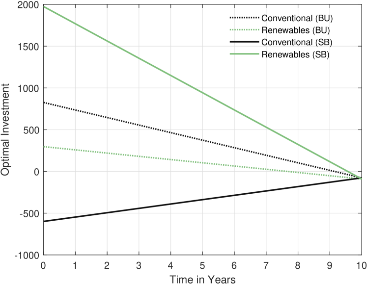
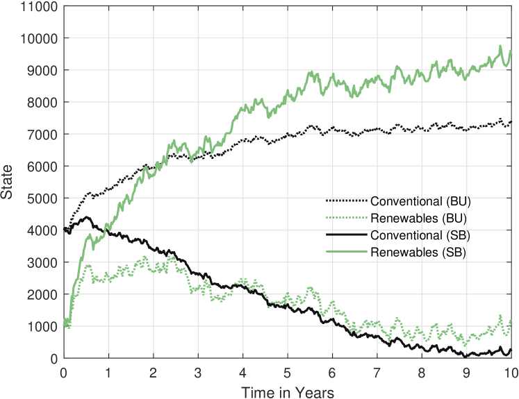
Figure 1 (a) illustrates the optimal investments in energy production capacity for the monopolist over time. In green, we see the optimal drift control for renewables $a_{2}^{\star,M}$ and for conventional energy $a_{1}^{\star,M}$ in black. The dotted lines represent the behaviors under business-as-usual (BU), while the solid lines refer to the second-best (SB) responses. We observe that the dotted lines are closer together and that in the business-as-usual case the conventional investments are always higher than the renewable ones. The business-as-usual investments decrease linearly over time but with different slopes. This phenomenon arrives since

$$\dot{{a}}_{j}^{BU,M}=-\frac{p(q_{i}-\varepsilon)}{Q_{M}}<0\;,\quad\quad\text{for }j=1,2,\quad j\neq i\;.$$ (3.1)

Since $\varepsilon<q_{1}<q_{2}$, the slope for conventional energy is more steep. In contrast, the second-best response for conventional energy is negative over the whole time horizon as $k_{1}<0$ and linearly increasing since

$$\dot{{a}}_{1}^{SB,M}=\frac{q_{2}}{Q_{M}}\dot{z}_{1}-\frac{\varepsilon}{Q_{M}}\dot{z}_{2}<0\;.$$ (3.2)

In contrast, renewable energy investments drastically increase due to $k_{2}>0$ and $\dot{{a}}_{2}^{SB,M}>0$. Note, that since $\delta_{1}=\delta_{2}=0$, the marginal optimal drift payments $\dot{z}_{1}$ and $\dot{z}_{2}$ become constant (see Remark 2.3). Moreover, we observe that the terminal controls, ${a}_{j}^{SB,M}(T)={a}_{j}^{BU,M}(T)$, coincide at terminal time since $z_{j}(T)=w^{A}_{j}(T)=0$ for $j=1,2$.

Figure 1 (b) illustrates the cumulative energy investments of the monopolist for renewable and conventional energy over time with drift control only. The effect of volatility control will be discussed in Section 3.2. The green and black trajectories depict renewable and conventional energy production capacity, respectively. The dotted lines again characterize the evolution in the business-as-usual setting and the solid lines specify the evolution under the second-best contract. We observe higher fluctuations for renewable investments than for conventional ones in both situations (business-as-usual and second-best) since $\sigma_{2}>\sigma_{1}$. In particular, the renewables’ volatility is more than twice as high as for conventional energy production. Regarding the progress over time, we observe a significant effect of the optimal drift response by the monopolist. Under business-as-usual, renewable investments initially sightly increase in the first years, stagnate and return to the initial production level in the end of the time horizon. Whereas the conventional energy production frequently increases over the whole time horizon. Under the second-best contract, we observe the contrary: Conventional energy production capacity decreases significantly during the contracting period. On the other hand, renewable energy becomes famous and significantly increases to the nine-fold of the initial investment level. However, energy production does not seem very stable in this situation, which motivates the introduction of volatility control investigated in the next section.

3.2 The Effect of Volatility Control

(a) Optimal volatility response under BU

(b) Optimal volatility response under SB

Figure 2: The monopolistic setting with volatility control. Subfigure (a): Monopolist’s optimal volatility control $b^{BU,M}$ in the business-as-usual case. Subfigure (b): Monopolist’s optimal volatility control $b^{SB,M}$ under the second-best contract.

(a) Investment effort

(b) State process

Figure 3: The monopolistic setting under the second-best contract with volatility control (DVC) and without volatility control (DC, i.e. constant uncontrolled volatilities $\sigma_{1}$ and $\sigma_{2}$ given by Table 1). Subfigure (a): Monopolist’s optimal investments $a^{SB,M}$ in energy production capacity. Subfigure (b): Energy production capacity in the monopolistic setting.

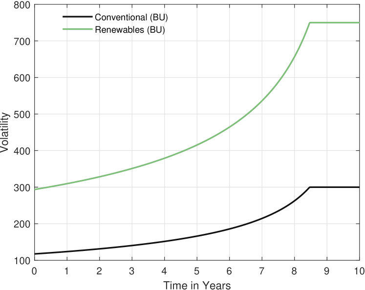
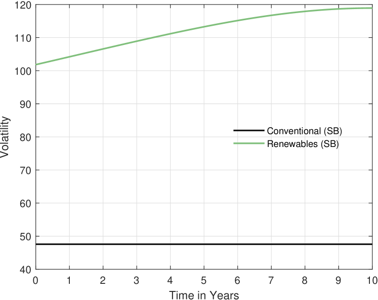
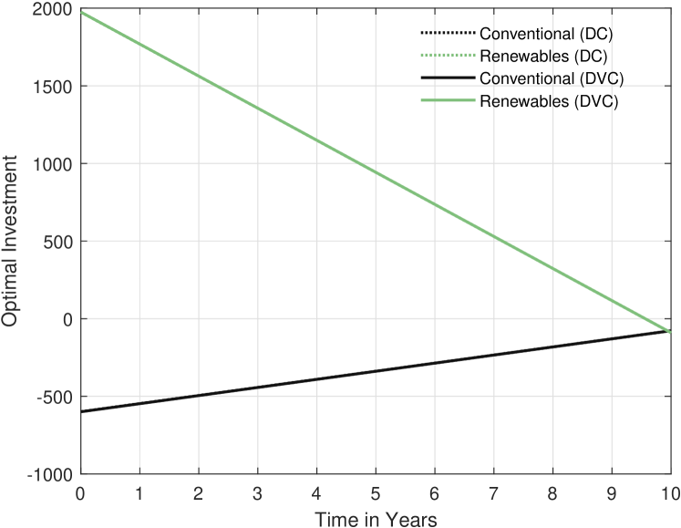
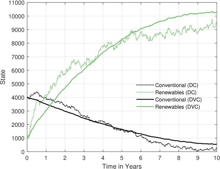
Figure 2 illustrates the monopolist’s volatility control in the business-as-usual case and under the second-best contract over the whole time horizon. The solid green lines refer to the controlled volatility of renewables. The solid black lines refer to the controlled volatility of conventional energy production capacity. We observe that all volatilities are on average lower than their upper boundaries. In both subfigures, the renewables come along with a higher volatility than the conventional energy, since $\Phi_{2}>\Phi_{1}$. However, we can identify two main differences: In Figure 2 (a), the volatilities for both energy sources are higher than under a second-best contract. In fact, they increase convexly until they are truncated by their upper boundaries $\sigma_{1}$ and $\sigma_{2}$ during the last two years when no efforts are made since the efforts become too costly. In contrast, Figure 2 (b) shows lower and thus untruncated volatilities. The second-best volatility for renewables results in the end approximately at the level of the business-as-usual volatility for conventional sources at initial time. Moreover, we observe a concave behavior for renewables’ volatility whereas the variability of conventional sources remain rather constant. This phenomenon arises as $\gamma_{1}$ stays nearly constant around $-h$ and $\gamma_{2}$ increases from $-1.9532e+09$ to $-h$.

The effect of volatility control on the drift control through the drift payment $z$ remains very small. In fact, Figure 3 (a) shows that the investment efforts under a second-best contract with and without volatility control are indistinguishable. Numerically, we observe that the effect under volatility control becomes more pronounced since $a_{1}^{SB,M,DVC}\leq a_{1}^{SB,M,DC}\leq a_{2}^{SB,M,DC}\leq a_{2}^{SB,M,DVC}$. However the maximal difference between the renewables is $0.3864$ MW and between the conventional energy $0.7640$ MW.

Figure 3 (b) clearly manifests the exclusive effect of volatility control. The solid lines display the state over time resulting from a second-best contract with volatility control whereas the dotted lines refer to the state resulting from a second-best contract without volatility control. We observe that the states are extremely smoothed by volatility incentives, due to the extremely lowered volatility (from $\sigma_{1}$ and $\sigma_{2}$ to Figure 2 (b)). Moreover, for both energy sources, we initially observe that volatility incentives lead on average to a smaller state. In the second half of the contracting period, we observe the contrary: The state is higher under volatility control than without volatility control.

3.3 The Effect of Competition

Figures 4 and 5 illustrate the optimal investments and the resulting state process without volatility control in the business-as-usual case (Figure 4) and under the second-best contract (Figure 5), respectively. As before, green lines refer to renewable energy and black lines are assigned to conventional energy. The dotted lines indicate a monopolistic market structure whereas the solid line indicates the competitive setting.

(a) Investment effort under BU

(b) State process under BU

Figure 4: A comparison of the market structures, monopolistic (M) and competitive (C), in the business-as-usual case without volatility control. Subfigure (a): Investment efforts $a^{BU,\cdot}$ for each market structure. Subfigure (b): Energy production capacity for each market structure.

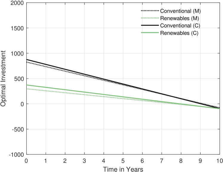
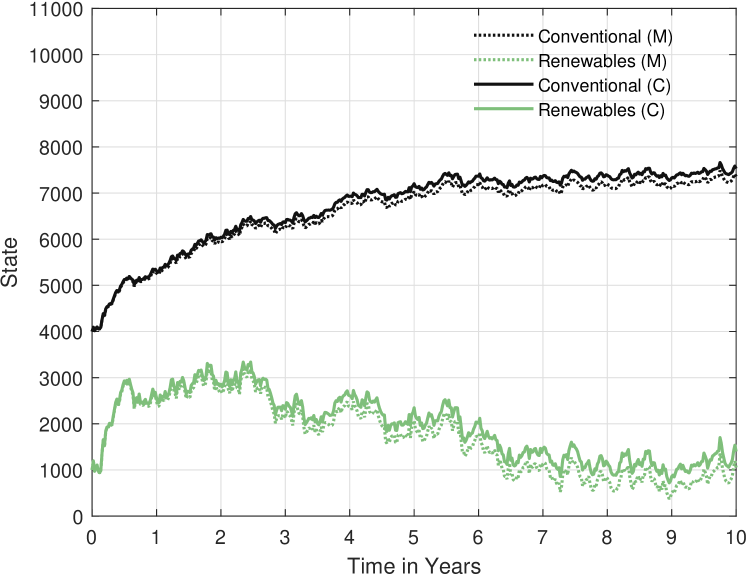
In Figure 4 (a), we observe different investment efforts in the absence of a contract even if the cost function of the competitors sum up to the cost function of the monopolist (especially the congestion costs $\varepsilon$ coincide). At the beginning of the contracting period, both market structures show positive investment efforts in both energy sources whereas we observe the contrary at the end of the time horizon. Nevertheless, the effect of the ladder time period does not translate into the state process (see Figure 4 (b)). The state is always greater or equal under a competitive market structure than under a monopolistic setting.

(a) Investment effort under SB

(b) State process under SB

Figure 5: A comparison of the market structures, monopolistic (M) and competitive (C), under a second-best contract without volatility control. Subfigure (a): Investment efforts $a^{SB,\cdot}$ for each market structure. Subfigure (b): Energy production capacity for each market structure.

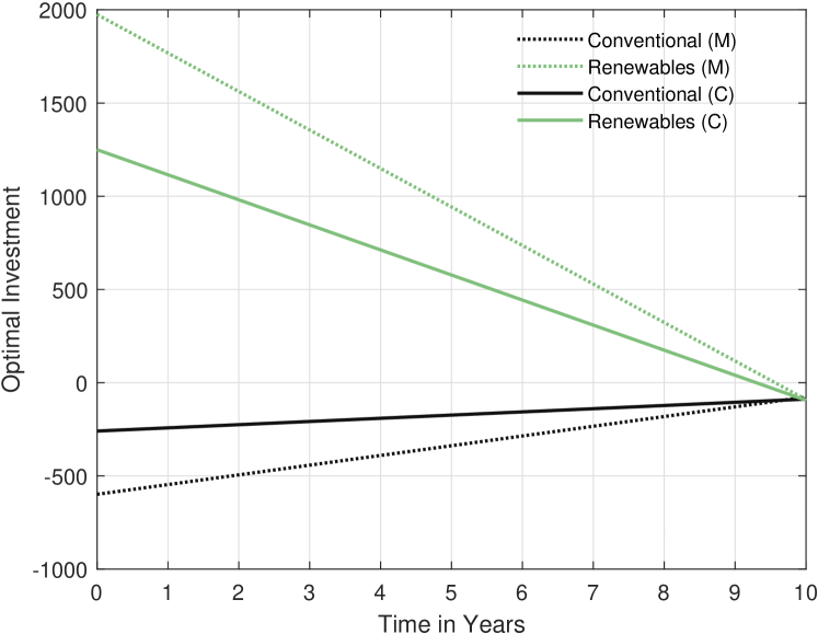
In the second-best case, the situation drastically changes. In contrast to the business-as-usual case, we now observe less pronounced investment efforts under competition (see Figure 5 (a)). In particular, we observe that $a_{1}^{SB,M}\leq a^{SB,1}\leq a^{SB,2}\leq a_{2}^{SB,M}$. This phenomenon arises through coupling at the level of the regulator’s drift payments, $z_{12}$ and $z_{21}$, under competition. The first competitor profits and the second competitor is harmed by the payments from the regulator.

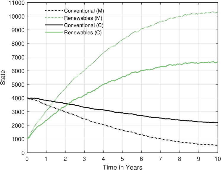
In Figure 5 (b), the effect of drift control translates into the state process such that the state under competition is less pronounced than under a monopolistic market structure. In particular, under competition, the terminal renewable production lies around 6,000 MW (whereas 9,000 MW is reached under a monopoly). The conventional energy production capacity only bisects to 2,000 MW under competition instead of falling below 200 MW in a monopolistic setting. Under competition, we thus observe less extreme trajectories and effects.

Both market structures indicate a higher volatility for renewable energy sources than for conventional ones. A joint effect of competition with volatility control will be investigated in the next section.

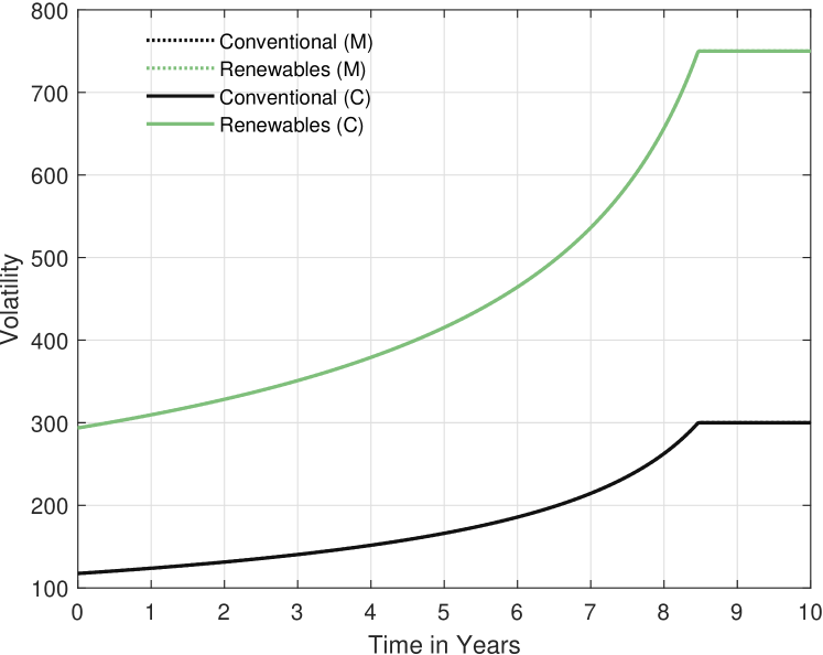
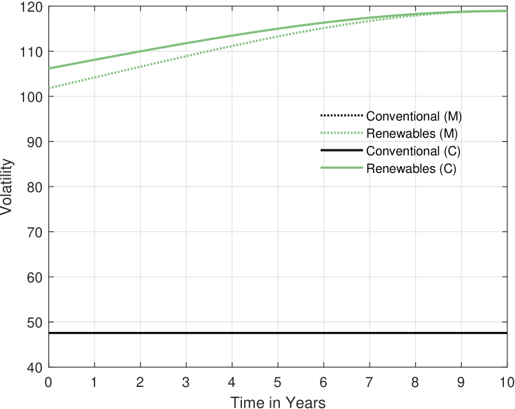
3.4 The Joint Effect of Competition and Volatility Control

In Figure 6, we consider the same setting as in Figure 2 in dotted lines and supplement the competitive setting in solid lines. In the absence of a contract, the optimal volatility responses coincide (see Figure 6 (a)), since ${b}_{j}^{BU,M}={b}^{BU,j}$ for $j=1,2$. However, under a second-best contract, the volatility efforts differ between the market structures (see Figure 6 (b)) as the volatility payments $\gamma_{j}\neq\gamma^{j}_{j}$ for $j=1,2$ do. For both energy sources, we find that ${b}_{j}^{SB,M}\leq{b}^{SB,j}$ since $\gamma_{j}\leq\gamma^{j}_{j}$ for $j=1,2$ for nearly the whole time horizon. For the last month only, this behavior changes to $\gamma^{j}_{j}<\gamma_{j}$ reaching $\gamma^{j}_{j}(T)<\gamma_{j}(T)=-h$ at terminal time for $j=1,2$.

From Figure 3, we already now that the effect of volatility efforts on the optimal investment level is very small. Hence, we refer to Figure 4 (a) and Figure 5 (a) for a comparison of optimal investments between the market structures in the case with and without a second-best contract, respectively.

(a) Optimal volatility response under BU

(b) Optimal volatility response under SB

Figure 6: A comparison of volatility controls for both market structures, monopolistic (M) and competitive (C). Subfigure (a): Optimal volatility in the business-as-usual case. Subfigure (b): Optimal volatility under the second-best contract.

(a) State process under BU

(b) State process under SB

Figure 7: A comparison of the energy production capacity with volatility control for both market structures, monopolistic (M) and competitive (C). Subfigure (a): Energy production capacity in the business-as-usual case. Subfigure (b): Energy production capacity under the second-best contract.

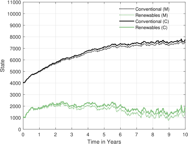
In Figure 7, we illustrate the development of energy production capacity with joint effects under business-as-usual and the second-best contract, respectively. Even in the absence of a contract (see Figure 7 (a)), the states under volatility control are slightly smoother than without volatility control (see Figure 4 (b)) due to the fact that the competitors are slightly encouraged to stabilize the production also in the absence of a contract.

In Figure 7 (b), the joint effect manifests more explicitly. We observe that the trajectories from Figure 5 (b) become a smoothed version (as in Figure 3 (b) for the monopolistic case). In fact, the dotted lines of Figure 7 (b) coincide with the solid lines from Figure 3 (b). We observe, as in Section 3.3, that competition leads to less pronounced capacity development. Moreover, as in Section 3.2, the ability of controlling the state’s variability leads to higher production capacity on the long-term than under drift control only.

3.5 A Comparison of the Overall Production Capacity

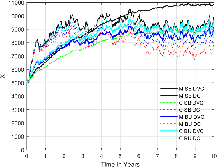
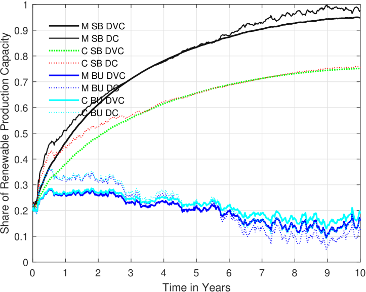
Figure 8 summarizes the development of the total energy production capacity and the share of renewables’ capacity for all scenarios resulting from different market structures (M and C), from business-as-usual and second-best contracts (BU and SB), and the absence and presence of volatility control (DC and DVC). In Figure 8 (a), all scenarios are endowed with a total initial production capacity of 5,000 MW and rise over the time horizon of ten years. On the long term, the monopolistic market structure regulated by the second-best contract outperforms all other scenarios with nearly 11,000 MW under drift and volatility control and approximately 10,000 MW under drift control only. The competitive setting with drift control only leads under the second-best contract to the lowest capacity with around 8,000 MW at the end of the contracting period. Competition under a second-best scenario with drift and volatility control is even in line with all business-as-usual scenarios on the long-term, however, with a drastic difference: the share of renewable energy production capacity in this regulated competitive setting is around 75% (in contrast to its business-as-usual scenario with approximately 17% share of renewables; see Figure 8 (b)). In a monopolistic market structure, the share is even higher at around 95% at the end of the contracting period (in contrast to its business-as-usual scenario with 14% share of renewables). Hence, this second-best contract is able to realize for example Germany’s 2030 target to triple renewables build-out by 2030. Without regulatory action the share of renewable production capacity remains below 20% on the long-term independent of the scenario.

(a) Total production capacity

(b) Share of renewables’ production capacity

Figure 8: Development of energy production capacity resulting from both market structures (M and C) with and without volatility control (DVC and DC) in the absence and presence of the second-best contract (BU and SB). Subfigure (a): Total energy production capacity. Subfigure (b): Share of renewables’ production capacity.

3.6 A Comparison of the Second-best Contracts

In Table 3, we observe the following ranking of contracts: $\xi_{M}^{DC}>\xi_{C,1}^{DC}+\xi_{C,2}^{DC}>\xi_{M}^{DVC}>\xi_{C,1}^{DVC}+\xi_{C,2}^{DVC}$. Hence, we find that the regulator pays more, whenever the volatility cannot be controlled since there are missing tax earnings in the uncontrolled settings. The scenario, in which the volatility can be controlled, is less expensive since the regulator taxes the variability of the production capacity.

Moreover, the sum of both competitive contracts is less expensive than the monopolist’s contract. This effect appears on the one hand through existing cross payments or charges, $z_{12}$ and $z_{21}$, respectively. On the other hand, interaction between the competitors diminishes the peculiarity of investment effects for which regulatory subsidies are paid or charges are taken, respectively. Hence, the monopolistic setting with more pronounced investment efforts are more costly for the regulator.

$\xi_{M}^{DC}$	$\xi_{M}^{DVC}$	$\xi_{C,1}^{DC}+\xi_{C,2}^{DC}$	$\xi_{C,1}^{DVC}+\xi_{C,2}^{DVC}$
4.24e+14	1.02e+14	3.77e+14	9.87e+13

Table 3: Total contract value paid by the regulator in the monopolistic (M) and competitive (C) setting under drift control only (DC) and with volatility control (DVC).

4 General Extended Linear-Quadratic Principal-Multi-Agent Model

In this section, we introduce the generalized incentive problem that $N$ competitive Agents and the Principal face. Each agent optimizes his own expected utility of the contract, offered by the Principal, and the corresponding payoff by choosing optimal actions. The Principal maximizes her own expected utility of the final payoff consisting of the contracts paid to the Agents and the Principal’s benefit attained under optimal response of the Agents.

4.1 The Model

The Agents’ controlled state process is denoted by $X=(X_{t})_{t\in[0,T]}$ and is the canonical process of the space $\Omega$ of $d-$dimensional continuous trajectories $w\colon[0,T]\to\mathbb{R}^{d}$, i.e. $X_{t}(\omega)=\omega(t)$ for all $(t,\omega)\in[0,T]\times\Omega$. $\mathbb{F}=\{\mathcal{F}_{t},t\in[0,T]\}$ denotes the corresponding filtration. The control processes of Agent $n=1,\ldots,N$ are a pair $(\alpha^{n},\beta^{n})=:\nu^{n}$ of $\mathbb{F}-$adapted processes. The drift control $\alpha^{n}\in A\subset\mathbb{R}^{d}$ refers to the Agent’s actions controlling the state’s mean-reversion level and $\beta^{n}\in B\subset\mathbb{R}^{d\times K}$ for $d\leq K$ is the action adjusting the state’s variability. The set of control processes is denoted by $\mathcal{U}$.

The State Process.

For a given initial state condition $X_{0}\in\mathbb{R}^{d}$, the state equation affected by $N$ Agents is given as a mean-reverting Ornstein-Uhlenbeck process

$$dX_{t}=\left(A_{0}X_{t}+\sum_{n=1}^{N}A_{n}\alpha^{n}_{t}\right)dt+\bar{\beta}_{t}dW_{t}\;,\quad\quad\bar{\beta}_{t}:=\sum_{n=1}^{N}\beta_{t}^{n}\;,\quad\quad t\in[0,T]\;,$$ (4.1)

driven by a $K-$dimensional Brownian motion $W$, where $A_{0},\ldots,A_{n}\in\mathbb{R}^{d\times d}$. We denote by $\mathbb{P}^{\nu}:=\mathbb{P}^{(\alpha,\beta)}$ the distribution of the state process $X$ corresponding to the control processes $\nu:=(\alpha,\beta)\in\mathcal{U}$. Let us denote the collection of all such measures $\mathbb{P}^{\nu}$ by $\mathcal{P}$. We assume that $K\geq d$, so that the control variables stay unobservable for the Principal. Indeed, consider for instance $d=1$, the Principal observes the quadratic variation of $d\langle X\rangle_{t}=\bar{\beta}_{t}\bar{\beta}_{t}^{\top}dt$ but she cannot recover the level of efforts $\bar{\beta}_{t}\in\mathbb{R}^{1\times K}$ unless $K=1$. The same remark generalizes when $d>1$.

The Agents’ Problems.

The objective function of Agent $n=1,\ldots,N$ is given by

$$J_{n}(\xi_{n},\mathbb{P}^{\nu})=\mathbb{E}^{\mathbb{P}^{\nu}}\left[U_{n}\left(\xi_{n}-\int_{0}^{T}C_{n}(\alpha_{t},\beta_{t},X_{t})dt\right)\right]\;,\text{ where }U_{n}(x)=-e^{-\eta_{n}x}\;,$$ (4.2)

for some constant risk aversion parameter $\eta_{n}>0$ and for a cost function given by

$$C_{n}(a,b,x)=c^{0}_{n}\cdot x+c^{\rm m}_{n}(a)+c^{\rm v}_{n}(b)\;,$$ (4.3)

where $c^{0}_{n}\in\mathbb{R}^{d}$, $c^{\rm v}_{n}\colon B^{N}\to\mathbb{R}_{+}$ is decreasing, convex for each component, $c^{\rm v}_{n}(0)=+\infty$, $c^{\rm v}_{n}(\sigma)=0$, and where

$$c^{\rm m}_{n}(a)=L^{n}\cdot a+\frac{1}{2}{\rm Tr}\left[aa^{\top}Q^{n}\right]\;,$$ (4.4)

with $L^{n}_{j}\in\mathbb{R}^{d},(Q^{n}_{ji})\in\mathbb{S}^{d}_{+}$ and $\mathcal{Q}:=(Q^{n}_{jn})_{nj}$ invertible. The cost $c_{n}^{\rm v}$ of volatility action $\beta$ prevents the Agent from eliminating the volatility since the cost would explode, and is equal to zero if the Agent makes no effort. For technical reasons, we need to consider bounded efforts and define the set of admissible controls as

$${{\color[rgb]{0,0,0}\definecolor[named]{pgfstrokecolor}{rgb}{0,0,0}\pgfsys@color@gray@stroke{0}\pgfsys@color@gray@fill{0}\mathcal{A}:=\left\{(\alpha^{n},\beta^{n})\text{ bounded for }n=1,\ldots,N\leavevmode\nobreak\ |\leavevmode\nobreak\ \beta\beta^{\top}\text{\leavevmode\nobreak\ invertible with bounded inverse}\right\}\;,}}$$ (4.5)

where the variances’s upper boundary $\sigma\sigma^{\top}$ refers to the case when no effort is made. The problem of Agent $n=1,\ldots,N$ is attained through

$$V_{n}(\xi_{n},\nu^{-n})=\sup_{\begin{subarray}{c}\nu^{n}\\ s.t.\leavevmode\nobreak\ \mathbb{P}^{\nu}\in\mathcal{P}\end{subarray}}J_{n}(\xi_{n},\mathbb{P}^{\nu})\;.$$ (4.6)

In particular, we want to find the Nash Equilibrium $\nu^{\star}$ by proceeding the following steps:

• Individual optimization for all $n=1,\ldots,N$ such that $\hat{\nu}^{n}(\nu^{-n})$ is the optimal response of Agent $n$.

• Nash Equilibrium for all $n=1,\ldots,N$ such that $\hat{\nu}^{n}((\nu^{\star})^{-n})=(\nu^{\star})^{n}$ is the optimal response of Agent $n$.

A control $\mathbb{P}^{\nu^{\star}}\in\mathcal{P}$ will be called optimal if $V_{n}(\xi_{n},(\nu^{\star})^{-n})=J_{n}(\xi_{n},\mathbb{P}^{\nu^{\star}})$, $\forall n=1,\ldots,N$. We denote the collection of all such optimal responses by $\mathcal{P}^{\star}(\xi)$. Whenever we consider second-best (SB) or business-as-usual (BU) optimal controls, we refer to SB or BU instead of indicating a star ($\star$). Moreover, we assume that the Agent $n=1,\ldots,N$ has a reservation utility $R_{0}^{n}\in\mathbb{R}_{-}$ and we denote by $E_{0}^{n}:=-\frac{1}{\eta_{n}}\ln(-R_{0}^{n})$, the certainty equivalent of the reservation utility of Agent $n$.

The Principal’s Problem.

The Principal’s objective function given $N$ individual contracts, denoted by $\xi=\left(\xi_{1},\ldots,\xi_{N}\right)^{\top}$, is given by

$$J_{P}(\xi,\mathbb{P}^{\nu})=\mathbb{E}^{\mathbb{P}^{\nu}}\left[U_{P}\left(-\sum_{n=1}^{N}\xi_{n}+\int_{0}^{T}\lambda\cdot X_{t}dt+\frac{1}{2}\int_{0}^{T}{\rm Tr}\left[g\leavevmode\nobreak\ d\langle X\rangle_{t}\right]+\Lambda\cdot X_{T}\right)\right]\;,$$ (4.7)

where $U_{P}(x)=-e^{-\eta_{P}x}$ for some constant risk aversion parameter $\eta_{P}>0$ and for $\lambda,\Lambda\in\mathbb{R}^{d}$, and $g\in\mathbb{R}^{d\times d}$. The resulting second-best problem is

$$V_{P}^{SB}=\sup_{{\xi\in\Xi}}\leavevmode\nobreak\ \sup_{\mathbb{P}^{\nu}\in\mathcal{P}^{\star}(\xi)}J_{P}(\xi,\mathbb{P}^{\nu})\;,$$ (4.8)

with the convention that $\sup\emptyset=-\infty$, so that we restrict the contracts that can be offered by the Principal to those $\xi\in\mathcal{C}$ such that $\mathcal{P}^{\star}(\xi)\neq\emptyset$, where $\Xi=\{\xi\in\mathcal{C}\colon V_{n}(\xi_{n},\nu^{-n})\geq R_{0}^{n},\forall\leavevmode\nobreak\ n=1,\ldots,N\}$ and $\mathcal{C}$ is the set of all $\mathcal{F}_{T}-$measurable random variables satisfying the integrability condition

$$\sup_{\mathbb{P}^{\nu}\in\mathcal{P}}\mathbb{E}^{\mathbb{P}^{\nu}}\left[e^{m\eta_{P}|\xi|}\right]+\sum_{n=1}^{N}\sup_{\begin{subarray}{c}\nu^{n}\\ s.t.\leavevmode\nobreak\ \mathbb{P}^{\nu}\in\mathcal{P}\end{subarray}}\mathbb{E}^{\mathbb{P}^{\nu}}\left[e^{-m\eta_{n}\xi_{n}}\right]<+\infty\;,\quad\text{for some }m>1\;,$$ (4.9)

such that the objectives of Principal and Agents are well-defined. We follow the standard convention in the Principal–Agent literature in the case of multiple optimal responses in $\mathcal{P}^{\star}(\xi)$, that the Agents implement the optimal response that is the best for the Principal.

Remark 4.1.

Note, that the Principal’s second-best problem in Equation (4.8) can be rewritten as

$$\sup_{\xi\in\mathcal{C}}J_{P}(\xi,\mathbb{P}^{\nu})\quad\text{s.t.}\quad(i)\leavevmode\nobreak\ V_{n}(\xi_{n},\nu^{-n})\geq R_{0}^{n}\;,\quad\forall n=1,\ldots,N\;,$$ (4.10)

$$(ii)\leavevmode\nobreak\ \mathbb{P}^{\nu}\in\mathcal{P}^{\star}(\xi)\;,$$ (4.11)

where $(i)$ is known as the participation constraint and $(ii)$ is the incentive constraint. In particular, $(ii)$ induces that the Agent desires to choose the optimal action when facing the incentive scheme which translates into Equation (4.6).

4.2 The Contract

Following Cvitanić et al.  (2018), the contract, the Principal offers to Agent $n$, can be reduced to the class of stochastic differential equation of the form

$$\xi_{n}=Y_{T}^{n,Z,\Gamma}=Y_{0}^{n}+\int_{0}^{T}Z_{t}^{n}\cdot dX_{t}+\frac{1}{2}\int_{0}^{T}{\rm Tr}\left[(\Gamma_{t}^{n}+\eta_{n}Z_{t}^{n}(Z_{t}^{n})^{\top})d\langle X_{\cdot}\rangle_{t}\right]-\int_{0}^{T}\mathcal{H}_{n}(X_{t},Z_{t},\Gamma_{t})dt\;,$$ (4.12)

extended to the Multi-Agent setting. Economically speaking, $Z$ and $\Gamma$ are the Principal’s payment rates corresponding to the variation of the state $X$ and its quadratic variation $\langle X\rangle$, which can be either payments ($Z,\Gamma>0$) or charges ($Z,\Gamma<0$). In particular, $Z^{n}\in\mathbb{R}^{d}$ and $\Gamma^{n}\in\mathbb{S}^{d}$ are the values Agent $n$ receives or pays. Moreover, the Principal pays a risk-compensation ($\eta_{n}Z^{n}(Z^{n})^{\top}$) to Agent $n$ since the Agent might suffer from managing the risky state $X$. Beyond these payments or charges, the contract for Agent $n$, denoted by $\xi_{n}$, induces a reduction by the Hamiltonian, i.e. by the Agent’s benefit of the contract over the contracting period. In particular, the Hamiltonian of Agent $n$ is defined by

$$\mathcal{H}_{n}(x,z^{n},\gamma^{n}):=\mathcal{H}_{n}^{0}(x,z^{n})+\mathcal{H}_{n}^{\rm m}(z^{n})+\mathcal{H}_{n}^{\rm v}(\gamma^{n})\;,$$ (4.13)

for $x\in\mathbb{R}^{d}$, for $z^{n}\in\mathbb{R}^{d}$, and for $\gamma^{n}\in\mathbb{S}^{d}$, where $\mathcal{H}_{n}^{0}$, $\mathcal{H}_{n}^{\rm m}$, and $\mathcal{H}_{n}^{\rm v}$ are the components of the Hamiltonian of Agent $n$ corresponding to the instantaneous state, mean-reversion level, and volatility, respectively:

$$\mathcal{H}_{n}^{0}(x,z^{n})=-c^{0}_{n}\cdot x+(A_{0}x)\cdot z^{n}\;,$$ (4.14)

$$\mathcal{H}_{n}^{\rm m}(z^{n})=\sup_{\alpha^{n}}-c^{\rm m}_{n}(\alpha)+\left(\sum_{j=1}^{N}A_{j}\alpha^{j}\right)\cdot z^{n}\;,$$ (4.15)

$$\mathcal{H}_{n}^{\rm v}(\gamma^{n})=\sup_{\beta^{n}}-c^{\rm v}_{n}(\beta)+\frac{1}{2}{\rm Tr}\left[(\bar{\beta}\bar{\beta}^{\top})\gamma^{n}\right]\;.$$ (4.16)

Lemma 4.1.

The value of Agent $n$ under the contract $\xi_{n}$ is given by $V_{n}(\xi_{n},\nu^{-n})=R_{0}^{n}\;,$ which is attained when the Hamiltonian from Equation (4.13) is optimized.

Proof. See Section A.1.

In particular, the Hamiltonian $\mathcal{H}_{n}$ describes the benefit, Agent $n$ earns resulting from the contract given the instantaneous payments $(z,\gamma)$ and the instantaneous state $x$. The variables $z^{n}$ and $\gamma^{n}$ represent the payments for Agent $n=1,\ldots,N$ for an adjusted behavior in drift and volatility, respectively. Given the instantaneous payments, each agent maximizes the instantaneous rate of benefit given by the Hamiltonian to deduce the optimal action on the mean-reversion level and on the volatility.

Assumption 4.1.

The volatility cost function $c_{n}^{\rm v}\colon B^{N}\to\mathbb{R}_{+}$ for $n=1,\ldots,N$ satisfies the following conditions:

• The minimizer of the optimization problem $\bar{c}^{\rm v}_{n}(\beta^{-n},b):=\inf_{\beta^{n}\colon\frac{1}{2}\bar{\beta}\bar{\beta}^{\top}=b}c_{n}^{\rm v}(\beta)$ exists,

• $\bar{c}^{\rm v}_{n}$ is differentiable with invertible gradient such that $\left(\nabla_{b}\bar{c}^{\rm v}_{n}\right)^{-1}\colon B^{N-1}\times\mathbb{S}^{d}\to\mathbb{R}^{d\times d}$ exists, and

• there exists a unique (up to a sign) solution $\beta^{\star,n}=\hat{\beta}^{n}(\beta^{\star,-n})$ to the system $\bar{\beta}\bar{\beta}^{\top}=2\left(\nabla_{b}\bar{c}^{\rm v}_{n}\right)^{-1}(\beta^{\star,-n},\gamma^{n})$.

Example 4.1 (Monopolistic Setup).

Let us consider the monopolistic setting from Section 2.1 with $N=1$ and $d=2$, where the volatility control $\beta^{M}=\begin{pmatrix}\beta_{1}^{M}&0\\ 0&\beta_{2}^{M}\end{pmatrix}=\bar{\beta}$ admits a cost function $c_{1}^{\rm v}(\beta)=\sum_{j=1}^{2}\phi_{j}(\beta_{j}^{M})$, for $\phi_{j}(\beta_{j}^{M})=((\beta_{j}^{M})^{-2}-\sigma_{j}^{-2})\Phi_{j}$ as in Equation (2.3). We assume that $\beta_{j}^{M}$ is bounded by $[\epsilon_{j},\sigma_{j}]$ for $\epsilon_{j}>0$ small and $j=1,2$. Hence, we can define for $\tilde{b}:=\begin{pmatrix}\tilde{b}_{1}&0\\ 0&\tilde{b}_{2}\end{pmatrix}$:

$$\bar{c}_{1}^{\rm v}(\tilde{b}):=\inf_{\beta^{M}\colon\frac{1}{2}\bar{\beta}\bar{\beta}^{\top}=\tilde{b}}\sum_{j=1}^{2}\phi_{j}(\beta_{j}^{M})=\sum_{j=1}^{2}\tilde{\phi}_{j}\left(\tilde{b}_{j}\right)\;,$$ (4.17)

for $\tilde{\phi}_{j}\left(\tilde{b}_{j}\right)=\left(\frac{1}{2}\tilde{b}_{j}^{-1}-\sigma_{j}^{-2}\right)\Phi_{j}$, for which the minimizer exists attained by $\tilde{b}_{j}=\frac{1}{2}\sigma_{j}^{2}$. Moreover, $\bar{c}_{n}^{\rm v}(\tilde{b})$ is differentiable since $\phi^{\prime}_{j}(\tilde{b}_{j})=-\frac{1}{2}\tilde{b}_{j}^{-2}\Phi_{j}$. For $g<0$, $\left(\phi_{j}^{\prime}\right)^{-1}(g)=\sqrt{\frac{\Phi_{j}}{-2g}}$. Hence, there exists a unique solution to the system $\bar{\beta}\bar{\beta}^{\top}=2\left(\nabla_{b}\bar{c}^{\rm v}_{n}\right)^{-1}(\gamma^{1})$ attained by $\beta_{j}^{M}(\gamma^{1})^{2}=2\sqrt{\frac{\Phi_{j}}{-2\gamma^{1}}}=\sqrt{\frac{2\Phi_{j}}{-\gamma^{1}}}$ for $j=1,2$. Note that this implies

$$\gamma^{1}=\nabla_{b}\sum_{j=1}^{2}\tilde{\phi}_{j}(\tilde{b}_{j})=\begin{pmatrix}\tilde{\phi}_{1}^{\prime}(\tilde{b}_{1})&0\\ 0&\tilde{\phi}_{2}^{\prime}(\tilde{b}_{2})\end{pmatrix}\;.$$ (4.18)

Example 4.2 (Competitive Setup).

Let us consider the competitive setting with $N=2$ and $d=2$ from Section 2.2, where the volatility control $\bar{\beta}=\begin{pmatrix}\beta^{1}&0\\ 0&\beta^{2}\end{pmatrix}$ admits a cost function $c_{j}^{\rm v}(\beta)=\phi_{j}(\beta^{j})$, for $\phi_{j}(\beta^{j})=((\beta^{j})^{-2}-\sigma_{j}^{-2})\Phi_{j}$ as in Equation (2.37). We assume that $\beta^{j}$ is bounded by $[\epsilon_{j},\sigma_{j}]$ for $\epsilon_{j}>0$ small and $j=1,2$. Hence, we can define for $\tilde{b}$ as in Example 4.1 and receive

$$\bar{c}_{j}^{\rm v}(\tilde{b}):=\inf_{\beta^{j}\colon\frac{1}{2}\bar{\beta}\bar{\beta}^{\top}=\tilde{b}}\phi_{j}(\beta^{j})=\tilde{\phi}_{j}(\tilde{b}_{j})\;,$$ (4.19)

such that we end up with the findings from Example 4.1. Note that this implies that

$$\gamma^{1}=\nabla_{b}\tilde{\phi}_{1}(\tilde{b}_{1})=\begin{pmatrix}\tilde{\phi}_{1}^{\prime}(\tilde{b}_{1})&0\\ 0&0\end{pmatrix}\;,\quad\quad\text{ and }\quad\quad\gamma^{2}=\nabla_{b}\tilde{\phi}_{2}(\tilde{b}_{2})=\begin{pmatrix}0&0\\ 0&\tilde{\phi}_{2}^{\prime}(\tilde{b}_{2})\end{pmatrix}\;.$$ (4.20)

4.3 The Agents’ Optimal Actions

We now focus on the Agents’ optimal actions. First, we consider the actions incentivized by the second-best contract. Then, we consider the business-as-usual behavior, i.e. the action without the presence of any contract. Afterwards, we compare the optimal actions resulting from both settings.

The following proposition provides the optimal actions of the Agents.

Proposition 4.1 (Agents’ best response).

Let Assumption 4.1 be satisfied. Then, the best individual response of Agent $n=1,\ldots,N$ to an instantaneous payment $z^{n}=(z^{n}_{1},\ldots,z^{n}_{d})^{\top}\in\mathbb{R}^{d}$ and $\gamma^{n}\in\mathbb{S}^{d}$ is determined through

$$\hat{\alpha}^{n}(\alpha^{-n},z^{n})=\left(Q^{n}_{nn}\right)^{-1}\left(A_{n}z^{n}-L^{n}_{n}-\sum_{j=1,j\neq n}^{N}Q^{n}_{jn}{\alpha}^{j}\right)\in\mathbb{R}^{d}\;,$$ (4.21)

which induce the unique equilibrium

$${\alpha}^{SB}(z)=\mathcal{Q}^{-1}\left(\textbf{AZ-L}\right)^{\top}\in\mathbb{R}^{dN}\;,\quad\quad\text{i.e.\ }\quad\quad{\alpha}^{SB,n}(z)=\sum_{l=1}^{N}(\mathcal{Q}^{-1})_{nl}(A_{l}z^{l}-L^{l}_{l})\;,$$ (4.22)

where $\mathcal{Q}:=(Q^{n}_{jn})_{1\leq n,j\leq N}$ and $\textbf{AZ-L}:=(A_{1}z^{1}-L^{1}_{1},\ldots,A_{N}z^{N}-L^{N}_{N})$ and $(\mathcal{Q}^{-1})_{nl}$ is the $n-$th block-column (of dimension $d$) and the $l-$th block-row (of dimension $d$) of the inverse of $\mathcal{Q}$. The optimal volatility control ${\beta}^{SB}(\gamma)$ can be determined by

$$\bar{\beta}^{SB}(\bar{\beta}^{SB})^{\top}=2(\nabla_{b}\bar{c}_{n}^{\rm v})^{-1}(\beta^{SB,-n},\gamma^{n})\;,$$ (4.23)

for which there exists a unique solution by Assumption 4.1.

Proof. See Section A.2.

The drift payment $z$ induces an effort of the Agent to adjust the mean-reversion level of the state. The volatility payment $\gamma$ induces an effort to adjust the state’s volatility. Next, we focus on the Agents’ actions without contract. The results are collected in the next proposition.

Proposition 4.2 (Agents’ behavior without contract).

Let Assumption 4.1 be satisfied. The optimal drift action of Agent $n=1,\ldots,N$ without contract is given by

$${\alpha}^{BU,n}({\alpha}^{-n},t)=\left(Q^{n}_{nn}\right)^{-1}\left(A_{n}w_{n}^{A}(t)-L^{n}_{n}-\sum_{j=1,j\neq n}^{N}Q^{n}_{jn}{\alpha}^{j}\right)\;,$$ (4.24)

where the marginal revenue function of Agent $n$, $w_{n}^{A}(t)$, is determined as the solution to

$$\dot{w}_{n}^{A}(t)=c^{0}_{n}-A_{0}\cdot w_{n}^{A}(t)\;,$$ (4.25)

subject to $w^{A}(T)=0$. Equation (4.24) can be rewritten in equilibrium as

$${\alpha}^{BU}(t)=\mathcal{Q}^{-1}\left(\bm{Aw^{A}(t)-L}\right)^{\top}\;,\quad\quad\text{i.e.\ }\quad\quad{\alpha}^{BU,n}(t)=\sum_{l=1}^{N}(\mathcal{Q}^{-1})_{nl}(A_{l}w_{l}^{A}(t)-L^{l}_{l})\;,$$ (4.26)

where $\mathcal{Q}:=\left(Q^{n}_{jn}\right)_{n,j}$ and $\bm{Aw^{A}(t)-L}:=(A_{1}w_{1}^{A}(t)-L^{1}_{1},\ldots,A_{N}w_{N}^{A}(t)-L^{N}_{N})$. The optimal volatility control ${\beta}^{BU,n}(t)$ is given as a solution to the system

$${{\color[rgb]{0,0,0}\definecolor[named]{pgfstrokecolor}{rgb}{0,0,0}\pgfsys@color@gray@stroke{0}\pgfsys@color@gray@fill{0}\bar{\beta}\bar{\beta}^{\top}=2(\nabla_{b}\bar{c}_{n}^{\rm v})^{-1}(\beta^{-n},-\eta_{n}w_{n}^{A}(t)w_{n}^{A}(t)^{\top})}}\;,$$ (4.27)

for which there exists a unique solution by Assumption 4.1.

Proof. See Section A.3.

Within the framework of Proposition 4.2, we determine the value function of Agent $n=1,\ldots,N$ attained by $V_{n}(0)=U_{n}\left(\int_{t}^{T}w_{0}^{BU,n}(s)ds+w_{n}^{A}(t)\cdot x\right)$, where

$$w_{0}^{BU,n}(t)=w_{n}^{A}(t)\cdot A_{n}{\alpha}^{BU,n}(t)-\frac{1}{2}\eta_{n}{\rm Tr}\left[(w_{n}^{A}(t)w_{n}^{A}(t)^{\top})\bar{{\beta}}^{BU}(t)\bar{{\beta}}^{BU}(t)^{\top}\right]-c^{\rm m}_{n}({\alpha}^{BU}(t))-c^{\rm v}_{n}({\beta}^{BU}(t))\;.$$ (4.28)

The optimal actions of the Agents in Equations (4.22) and (4.26) differ in the type of drift payment only. In the business-as-usual case, the Agents receive $w^{A}$, instead of the payment $z$, attained as the solution of a system of first order ODEs in Equation (4.25).

Remark 4.2.

Comparing the optimal drift behaviors of Agent $n$ in Equations (4.22) and (4.26) corresponding to the cases with and without contract, we observe that they differ in $z$ and $w^{A}$ only. Hence, if at time $t\in[0,T]$ $z^{n}<w_{n}^{A}(t)$ for all $n=1,\ldots,N$, then $\alpha^{BU}(t)>\alpha^{SB}(t)$.

4.4 The Second-best Contracts

The full characterization of the optimal second-best contract is provided in the next proposition, for which we first introduce new notation and make the following assumptions:

Assumption 4.2.

The volatility cost function $c_{n}^{\rm v}\colon B^{N}\to\mathbb{R}_{+}$ for $n=1,\ldots,N$ satisfies the following conditions:

• The minimizer of the optimization problem $\bar{f}_{n}(\beta^{\star,-n},b):=\inf_{\gamma\colon\frac{1}{2}\bar{\beta}^{\star}(\bar{\beta}^{\star})^{\top}=b}\sum_{n=1}^{N}c_{n}^{\rm v}(\beta^{\star}(\gamma))$ exists,

• $\bar{f}_{n}$ is differentiable with invertible gradient such that $\left(\nabla_{b}\bar{f}_{n}\right)^{-1}\colon B^{N-1}\times\mathbb{R}^{d\times d}\to\mathbb{S}^{d}$ exists, and

• there exists a unique (up to a sign) solution $\beta^{\star,n}=\hat{\beta}^{n}(\beta^{\star,-n})$ to the system $\bar{\beta}\bar{\beta}^{\top}=2\left(\nabla_{b}\bar{f}_{n}\right)^{-1}(\beta^{\star,-n},M)$.

Notation.

We define the following variables:

$$\zeta_{n}(\gamma):=(\eta_{n}+\eta_{P})\bar{{\beta}}^{SB}(\gamma)\bar{{\beta}}^{SB}(\gamma)^{\top}+A_{n}^{\top}\sum_{i,j,l=1}^{N}(\mathcal{Q}^{-1})_{jn}^{\top}Q^{l}_{ji}(\mathcal{Q}^{-1})_{in}A_{n}\;,$$ (4.29)

$$\mathcal{Z}^{w}_{n}(\gamma):=\eta_{P}\bar{{\beta}}^{SB}(\gamma)\bar{{\beta}}^{SB}(\gamma)^{\top}+\sum_{j=1}^{N}\left(A_{j}(\mathcal{Q}^{-1})_{jn}A_{n}\right)^{\top}\;,$$ (4.30)

$$\mathcal{Z}^{z}_{h,n}(\gamma):=\eta_{P}\bar{\beta}^{SB}(\gamma)\bar{\beta}^{SB}(\gamma)^{\top}+A_{n}^{\top}\sum_{i,j,l=1}^{N}(\mathcal{Q}^{-1})_{jn}^{\top}Q_{ji}^{l}(\mathcal{Q}^{-1})_{ih}A_{h}\;,\quad\text{ for }h\neq n\;,$$ (4.31)

$$\mathcal{Z}^{c}_{n}:=A_{n}^{\top}\sum_{i,j,k,l=1}^{N}(\mathcal{Q}^{-1})_{jn}^{\top}\left(L^{k}_{j}-Q_{ji}^{k}(\mathcal{Q}^{-1})_{il}L_{l}^{l}\right)\;,$$ (4.32)

$$\hat{\mathcal{M}}(z,t):=g-\sum_{n=1}^{N}\eta_{n}z^{n}(z^{n})^{\top}-\eta_{P}\left(w^{P}(t)-\sum_{n=1}^{N}z^{n}\right)\left(w^{P}(t)-\sum_{n=1}^{N}z^{n}\right)^{\top}\;,$$ (4.33)

where $w^{P}(t)$ is a solution to the system of ODEs $\dot{w}^{P}(t)=-\left(\lambda-\sum_{n=1}^{N}c^{0}_{n}\right)-w^{P}(t)\cdot A_{0}$, subject to $w^{P}(T)=\Lambda$.

Proposition 4.3 (Second-best contract).

Let Assumptions 4.1 and 4.2 be satisfied.

1. The optimal payment for the drift and volatility controls, $z(t)$ and $\gamma(t)$, are deterministic functions given as solutions to the system of nonlinear equations:

   $$z(t)=(\mathcal{Z}^{z})^{-1}\left(\bm{\mathcal{Z}^{w}(\gamma)w^{P}(t)-\mathcal{Z}^{c}}\right)\in\mathbb{R}^{dN}\;,$$ (4.34)

   $$\left(\nabla_{b}\bar{c}_{n}^{\rm v}\right)^{-1}\left(\beta^{\star,-n}(\gamma),\gamma^{n}\right)=\left(\nabla_{b}\bar{f}_{n}\right)^{-1}\left(\beta^{\star,-n}(\gamma),\hat{\mathcal{M}}(z,t)\right)\;,\quad\forall n=1,\ldots,N\;,$$ (4.35)

   where $\bm{\mathcal{Z}^{w}(\gamma)w^{P}(t)-\mathcal{Z}^{c}}:=\left(\mathcal{Z}^{w}_{1}(\gamma)w^{P}(t)-\mathcal{Z}^{c}_{1},\ldots,\mathcal{Z}^{w}_{N}(\gamma)w^{P}(t)-\mathcal{Z}^{c}_{N}\right)^{\top}$ and $\mathcal{Z}^{z}_{n,n}(\gamma)=\zeta_{n}(\gamma)$, $\mathcal{Z}^{z}:=(\mathcal{Z}^{z}_{jn})_{1\leq n,j\leq N}$. Moreover, the Principal’s marginal revenue function, $w^{P}(t)$, is a solution to the following system of ODEs $\dot{w}^{P}(t)=-\left(\lambda-\sum_{n=1}^{N}c^{0}_{n}\right)-w^{P}(t)\cdot A_{0}$, subject to $w^{P}(T)=\Lambda$.

2. The second-best optimal contract is given by $\xi_{n}=\xi_{n}^{F}+\xi_{n}^{V}$, where

   $$\xi_{n}^{F}=U_{n}^{-1}(R_{0}^{n})-\int_{0}^{T}\mathcal{H}_{n}^{0}(X_{0},z(t))+\mathcal{H}_{n}^{\rm m}(z(t))+\mathcal{H}_{n}^{\rm v}(\gamma(t))dt\;,$$ (4.36)

   $$\xi_{n}^{V}=\int_{0}^{T}\pi_{n}^{D}(t)\cdot(X_{t}-X_{0})dt+\frac{1}{2}\sum_{i,j=1}^{d}\int_{0}^{T}\pi_{n,ij}^{V}(t)d\langle X^{i}_{\cdot},X^{j}_{\cdot}\rangle_{t}+(X_{T}-X_{0})\cdot z^{n}(T)\;,$$ (4.37)

   where for $n=1,\ldots,N$ and $i,j=1,\ldots,d$ the second-best optimal prices are attained by

   $$\pi_{n}^{D}(t)=-\dot{z}^{n}(t)+c^{0}_{n}-A_{0}z^{n}(t)\;,\quad\quad\pi_{n,ij}^{V}(t)=\gamma^{n}_{ij}(t)+\eta_{n}z^{n}_{j}(t)z^{n}_{i}(t)\;.$$ (4.38)

Proof. See Section A.4.

The second-best contract admits a form of a rebate contract: Agent $n$ gets a fixed payment $\xi^{F}_{n}$ consisting of his certainty equivalent of the reservation utility minus the benefit he would earn if no effort is made. Beyond, Agent $n$ is paid a variable payment $\xi_{n}^{V}$ covered by a second-best optimal drift price paid for each deviation from the initial state value and a second-best optimal volatility price proportional to the states’ covariation plus a terminal bonus for the final difference to the baseline.

In particular, $\pi_{n}^{D}$ and $\pi_{n}^{V}$ are the second-best prices for the state and its variability, respectively. This form is a rebate contract, where $X_{0}$ serves as a baseline.

Within the setting of Proposition 4.3, we can determine the Principal’s second-best value function in Equation (4.8). It is attained by $V_{P}^{SB}=U_{P}\left(-\sum_{n=1}^{N}E_{0}^{n}+v^{SB}(0,X_{0})\right)$ where

$$v^{SB}(t,x)=\int_{t}^{T}w^{P}_{0}(s)ds+w^{P}(t)\cdot x\;,$$ (4.39)

characterized through

$$w^{P}_{0}(t)=-\inf_{{z}}\Bigg{\{}-w^{P}(t)\cdot\sum_{n=1}^{N}A_{n}{\alpha}_{n}^{SB}(z)+\sum_{n=1}^{N}C_{n}({\alpha}^{SB}(z))-f^{\star}(\hat{\mathcal{M}}(z,t))\Bigg{\}}\;,$$ (4.40)

$$f^{\star}(M):=\sup_{b\geq 0}\left\{{\rm Tr}\left[bM\right]-\bar{f}_{n}(\beta^{\star,-n}(\gamma),b)\right\}\;.$$ (4.41)

4.5 Economic Analysis

Note, that if $N=1$ or if $c_{n}^{\rm v}(\beta^{\star})=c_{n}^{\rm v}(\beta^{\star,n})$ for all $n=1,\ldots,N$, then the optimal volatility payment deduced from Equation (4.35) reduces to $\gamma^{n}(t)=\hat{\mathcal{M}}(z,t)$, $\forall n=1,\ldots,N$. Hence, $\hat{\mathcal{M}}$ is the volatility payment matrix excluding all interaction costs the Agent may experience. In the monopolistic case (see Section 2.1) and in the competitive case without volatility interaction (see Section 2.2) the volatility payments become more explicit. We refer to Propositions 2.3 and 2.7 for more details.

If we assume, that there is only one agent without volatility control (i.e. $\bar{\beta}=\sigma$), without costs in the state (i.e. $c^{0}_{n}=(0,\ldots,0^{\top}$), and the state does not induce any mean-reversion (i.e. $A_{0}=(0,\ldots,0)^{\top}$), then we have the following results for the optimal contract $\xi_{1}=\xi_{1}^{F}+\xi_{1}^{V}$ offered to the Agent:

$$\xi_{1}^{F}= \leavevmode\nobreak\ U_{1}^{-1}(R_{0}^{1})-\int_{0}^{T}\mathcal{H}_{1}^{\rm m}(z(t))dt+\frac{1}{2}\int_{0}^{T}\pi_{1}^{V}(t)\sigma\sigma^{\top}dt\;,$$ (4.42)

$$\xi_{1}^{V}= \int_{0}^{T}\pi_{1}^{D}(t)\cdot(X_{t}-X_{0})dt+(X_{T}-X_{0})\cdot z^{1}(T)\;,$$ (4.43)

where $\pi_{1}^{D}(t)=-\dot{z}^{1}(t)=\lambda\mathcal{Z}\;,\leavevmode\nobreak\ \pi_{1}^{V}(t)=\eta_{1}z^{1}(t)z^{1}(t)^{\top}$. Note that under those assumptions $\mathcal{H}_{1}^{0}(x,z)=0$ and that the drift payment to the Agent is given by $z^{1}(t)=\mathcal{Z}w^{P}(t)\in\mathbb{R}^{d}$, where

$$\mathcal{Z}=\Big{[}(\sigma\sigma^{\top})(\eta_{1}+\eta_{P})+A_{1}^{\top}(Q^{1}_{11})^{-1}A_{1}\Big{]}^{-1}\left((\sigma\sigma^{\top})\eta_{P}+A_{1}^{\top}(Q^{1}_{11})^{-1}A_{1}\right)\;,$$ (4.44)

$$w^{P}(t)=\lambda(T-t)+\Lambda\;,$$ (4.45)

$${\alpha}_{1}^{SB}(z^{1})=(Q^{1}_{11})^{-1}(A_{1}z^{1}-L_{1}^{1})\;,$$ (4.46)

$$\hat{\mathcal{M}}(z^{1},t)=g-\eta_{1}z^{1}(z^{1})^{\top}-\eta_{P}\left(w^{P}(t)-z^{1}\right)\left(w^{P}(t)-z^{1}\right)^{\top}\;.$$ (4.47)

Hence, all expressions become more explicit and very similar to the results without responsiveness incentives of Aïd et al.  (2022). The contract still splits into the fixed and variable part, $\xi_{1}^{F}$ and $\xi_{1}^{V}$. However, Equation (4.43) contains a terminal bonus since $z(T)\neq 0$. If we set the terminal bonus $\Lambda$ to zero, the term disappears and the contract has the same structure as Aïd et al.  (2022) (up the multi-dimensional notation).

If the Agent is risk-neutral (but still with unobservable efforts), then we are in the first-best optimum in which the Principal can achieve the same level of utility as with the first-best contract with observable efforts but under a different type of contract. This means that the drift payment is directly $z^{1}(t)=w^{P}(t)$. Moreover, the optimal second-best prices reduce to $\pi_{1}^{D}(t)=\lambda$ and $\pi_{1,ij}^{V}(t)=0$ for $i,j=1,\ldots,d$.

To ensure readability, our setting excludes any discount factors. As in Cvitanić et al.  (2018), an extension to a discounted setting with the objective of the $n-$th Agent of the form

$$J_{n}(\xi_{n},\mathbb{P}^{\nu})=\mathbb{E}^{\mathbb{P}^{\nu}}\left[U_{n}\left(re^{-rT}\xi_{n}-\int_{0}^{T}re^{-rt}C_{n}(\alpha_{t},\beta_{t},X_{t})dt\right)\right]\;,\text{ where }U_{n}(x)=-e^{-\eta_{n}x}\;,$$ (4.48)

can be achieved by modifying the contract to

$$\xi_{n}=Y_{T}^{n,Z,\Gamma}=Y_{0}^{n}+\int_{0}^{T}Z_{t}^{n}\cdot dX_{t}+\frac{1}{2}\int_{0}^{T}{\rm Tr}\left[(\Gamma_{t}^{n}+re^{-rt}\eta_{n}Z_{t}^{n}(Z_{t}^{n})^{\top})d\langle X\rangle_{t}\right]-\int_{0}^{T}\mathcal{H}_{n}(X_{t},Z_{t},\Gamma_{t})-rY_{t}dt\;.$$

5 Conclusion

In this paper, we considered general Principal-Multi-Agent incentive problems with hidden drift and volatility actions and a lump-sum payment at the end of the contracting period. The contribution is twofold: first, we show how to increase investments in renewable energy while simultaneously ensuring stable energy production in a monopolistic and in an interacting setting with two agents. Second, we expand both models to a general interacting setting that still leads to closed-form solutions for the optimal contract being of rebate form. The numerical study highlights the impact of the contract design on the investments in (non-)renewable energy production capacity. This will lead to significant benefits for the regulator as well as to great adjustments in average investment and responsiveness of the power producer.

Appendix A Appendix – Proofs for Section 4

For notational conveniance, we skip the index regarding second-best (SB) and business-as-usual (BU) and indicate the equilibrium with a star ($\star$).

A.1 Agent’s Value of the Contract (Lemma 4.1)

Plugging contract $\xi_{n}$ from Equation (4.12) into $V_{n}(\xi_{n},\nu^{-n})$ gives us

$$V_{n}(Y_{0},Z,\Gamma,\nu^{-n})=-U_{n}(Y_{0}^{n})\sup_{\begin{subarray}{c}\nu^{n}\;,\\ \text{s.t.\leavevmode\nobreak\ }\mathbb{P}^{\nu}\in\mathcal{P}\end{subarray}}\mathbb{E}^{\mathbb{P}^{\nu}}\left[U_{n}\left(L_{T}\right)\right]\;,$$ (A.1)

where $dL_{t}=Z_{t}^{n}\cdot dX_{t}+\frac{1}{2}{\rm Tr}\left[(\Gamma_{t}^{n}+\eta_{n}Z_{t}^{n}(Z_{t}^{n})^{\top})d\langle X\rangle_{t}\right]-\mathcal{H}_{n}(X_{t},Z_{t},\Gamma_{t})dt-C_{n}(\alpha_{t},\beta_{t},X_{t})dt$ with $L_{0}=0$.

Note, that for $G_{T}:=U_{n}\left(L_{T}\right)=-1+\int_{0}^{T}dG_{t}$ we have

$$dG_{t} =dU_{n}(L_{t})=-\eta_{n}U_{n}(L_{t})dL_{t}+\frac{1}{2}\eta_{n}^{2}U_{n}(L_{t})d\langle L_{\cdot}\rangle_{t}\;.$$ (A.2)

Hence, we can follow

$$\mathbb{E}^{\mathbb{P}^{\nu}}\left[U_{n}\left(L_{T}\right)\right]$$

$$= \leavevmode\nobreak\ \mathbb{E}^{\mathbb{P}^{\nu}}\left[-1-\int_{0}^{T}U_{n}(L_{t})\eta_{n}dL_{t}+\frac{1}{2}\int_{0}^{T}{\rm Tr}\left[\eta_{n}^{2}U_{n}(L_{t})d\langle L_{\cdot}\rangle_{t}\right]\right]$$

$$= \leavevmode\nobreak\ \mathbb{E}^{\mathbb{P}^{\nu}}\Bigg{[}-1-\int_{0}^{T}U_{n}(L_{t})\eta_{n}\Bigg{(}Z_{t}^{n}\cdot\left(A_{0}X_{t}+\sum_{n=1}^{N}A_{n}\alpha_{t}^{n}\right)+\frac{1}{2}{\rm Tr}\left[\eta_{n}\Gamma_{t}^{n}\left(\bar{\beta}\bar{\beta}^{\top}\right)\right]-C_{n}(\alpha_{t},\beta_{t},X_{t})-\mathcal{H}_{n}(X_{t},Z_{t},\Gamma_{t})\Bigg{)}dt\Bigg{]}$$

$$\leq -1\;.$$

The supremum is exactly attained for $\nu$ being the optimal solution of the Hamiltonian. Hence,

$$\sup_{\begin{subarray}{c}\nu^{n}\;,\\ \text{s.t.\leavevmode\nobreak\ }\mathbb{P}^{\nu}\in\mathcal{P}\end{subarray}}\mathbb{E}^{\mathbb{P}^{\nu}}\left[U_{n}\left(L_{T}\right)\right]=U_{n}(Y_{0}^{n})\;,$$ (A.3)

subject to $V_{n}(\xi_{n},\nu^{-n})\geq R_{0}^{n}$ due to the participation constraint. By Karush-Kuhn-Tucker the equality follows.

A.2 Agent’s Best Response (Proposition 4.1)

Taking FOC in the Pre-Hamiltonian regarding the drift control of Agent $n$ and setting to zero gives us

$$A_{n}z^{n}=L^{n}_{n}+\sum_{j=1}^{N}Q_{jn}^{n}\alpha^{j}\;,$$ (A.4)

which equals Equation (4.22) in matrix style. Collecting terms regarding $\alpha^{n}$ gives Equation (4.21).

The Hamiltonian part of instantaneous volatility of Agent $n$ can be rewritten in terms of

$$\mathcal{H}_{n}^{\rm v}(\gamma^{n})=\sup_{b\geq 0}\left\{\sup_{\beta^{n}\colon b=\frac{1}{2}\bar{\beta}\bar{\beta}^{\top}}\left\{\frac{1}{2}{\rm Tr}[(\bar{\beta}\bar{\beta}^{\top})\gamma^{n}]-c_{n}^{\rm v}(\beta)\right\}\right\}=\sup_{b\geq 0}\left\{{\rm Tr}[b\gamma^{n}]-\inf_{\beta^{n}\colon b=\frac{1}{2}\bar{\beta}\bar{\beta}^{\top}}\left\{c_{n}^{\rm v}(\beta)\right\}\right\}\;.$$ (A.5)

Rewriting in terms of Karush-Kuhn-Tucker ($\bar{c}_{n}^{\rm v}(\beta^{-n},b)=\inf_{\beta^{n}\colon b=\frac{1}{2}\bar{\beta}\bar{\beta}^{\top}}\left\{c_{n}^{\rm v}(\beta)\right\}=\inf_{\beta^{n}}\left\{c_{n}^{\rm v}(\beta)+\mathcal{L}(b-\frac{1}{2}\bar{\beta}\bar{\beta}^{\top})\right\}$) and taking FOC gives the Lagrange multiplier $\mathcal{L}^{\star}=\frac{1}{\bar{\beta}}\frac{\partial}{\partial\beta^{n}}c_{n}^{\rm v}(\beta)$. FOC with respect to $b$ and setting to zero gives us (4.23). Moreover, taking directly FOC to $\sup_{b\geq 0}\left\{{\rm Tr}[b\gamma^{n}]-\bar{c}_{n}^{\rm v}(\beta^{-n},b)\right\}$ gives $\gamma^{n}=\nabla_{b}\bar{c}_{n}^{\rm v}(\beta^{-n},b)$ and thus $\bar{\beta}\bar{\beta}^{\top}=2(\nabla_{b}\bar{c}_{n}^{\rm v})^{-1}(\beta^{-n},\gamma^{n})$. By Assumption 4.1, there exists a unique solution.

A.3 Agent’s Behavior without Contract (Proposition 4.2)

Step 1.

The value function of Agent $n\in\{1,\ldots,N\}$ is $V_{n}(0)=-e^{-\eta_{n}v^{n}(0,X_{0})}$. In particular, we have $u^{n}(t,x)=-e^{-\eta_{n}v^{n}(t,x)}$. The corresponding PDE is attained by

$$-\partial_{t}u^{n}=\sup_{\nu^{n}}\Big{\{}u^{n}_{x}\left(A_{0}x+\sum_{n=1}^{N}A_{n}\alpha^{n}\right)+{\rm Tr}\left[\frac{1}{2}u^{n}_{xx}\bar{\beta}\bar{\beta}^{\top}\right]+u^{n}\eta_{n}C_{n}(\alpha,\beta,x)\Big{\}}\;.$$ (A.6)

Plugging the structure of $u^{n}$ inside, we receive the certainty equivalent $v^{n}(t,x)$ as a solution to

$$-\partial_{t}v^{n}=\sup_{\nu^{n}}\Bigg{\{}v^{n}_{x}\cdot\left(A_{0}x+\sum_{n=1}^{N}A_{n}\alpha^{n}\right)+\frac{1}{2}{\rm Tr}\left[(v^{n}_{xx}-\eta_{n}v_{x}^{n}(v_{x}^{n})^{\top})\bar{\beta}\bar{\beta}^{\top}\right]-C_{n}(\alpha,\beta,x)\Bigg{\}}\;,$$ (A.7)

subject to $v^{n}(T,\cdot)=0$.

Step 2.

The optimal drift action of Agent $n\in\{1,\ldots,N\}$ without contract is attained by FOC regarding Equation (A.7), which gives $A_{n}v_{x}^{n}=L^{n}_{n}+\sum_{j=1}^{N}Q_{jn}^{n}\alpha^{j}$. Hence, the optimal response of Agent $n$ is given by

$$\hat{\alpha}^{n}(a^{-n},v_{x})=\left(Q^{n}_{nn}\right)^{-1}\left(A_{n}v_{x}^{n}-L^{n}_{n}-\sum_{j=1,j\neq n}^{N}Q^{n}_{jn}{\alpha}^{j}\right)\;,$$ (A.8)

which can be rewritten in equilibrium as

$${\alpha}^{\star}(z)=\mathcal{Q}^{-1}\left(\bm{Av_{x}-L}\right)^{\top}\;,$$ (A.9)

where $\mathcal{Q}:=\left(Q^{n}_{jn}\right)_{n,j}$ and $\bm{Av_{x}-L}:=(A_{1}v_{x}^{1}-L^{1}_{1},\ldots,A_{N}v_{x}^{N}-L^{N}_{N})$.

Similar to Proposition 4.1, we can derive the optimal volatility control from Equation (A.7) by considering the volatility part only:

$$\sup_{\beta^{n}}\Bigg{\{}\frac{1}{2}{\rm Tr}\left[(v^{n}_{xx}-\eta_{n}v_{x}^{n}(v_{x}^{n})^{\top})\bar{\beta}\bar{\beta}^{\top}\right]-c_{n}^{\rm v}(\beta)\Bigg{\}}\;.$$ (A.10)

By Assumption 4.1, there exists a unique solution. Hence, the optimal volatility control is determined through

$$\bar{\beta}\bar{\beta}^{\top}=2(\nabla_{b}\bar{c}_{n}^{\rm v})^{-1}(\beta^{-n},v_{xx}^{n}-\eta_{n}v_{x}^{n}(v_{x}^{n})^{\top})\;.$$ (A.11)

Step 3.

The solution of the PDE (A.7) is attained by the following certainty equivalent function

$$v^{n}(t,x)=\int_{t}^{T}w_{0}^{BU,n}(s)ds+w_{n}^{A}(t)\cdot x\;.$$ (A.12)

By directly plugging the guess (A.12) in the PDE (A.7), we obtain

$$w_{0}^{BU,n}(t)-\dot{w}^{BU,n}(t)\cdot x= \leavevmode\nobreak\ w_{n}^{A}(t)\cdot\left(A_{0}x+\sum_{n=1}^{N}A_{n}{\alpha}^{\star,n}(w_{n}^{A}(t))\right)$$

$$\leavevmode\nobreak\ -\frac{1}{2}{\rm Tr}\left[\eta_{n}w_{n}^{A}(t)(w_{n}^{A}(t))^{\top}\bar{{\beta}}^{\star}(\bar{{\beta}}^{\star})^{\top}\right]-C_{n}({\alpha}^{\star},{\beta}^{\star},x)\;,$$

from which we receive (4.28) and (4.25) when collecting terms regarding $x$.

A.4 Second-best Contract (Proposition 4.3)

Step 1.

The Principal’s second-best value function is attained by

$$V^{P}_{SB}=\sup_{Z,\Gamma}\mathbb{E}^{\mathbb{P}^{\nu^{\star}}}\left[e^{-\eta_{P}\int_{0}^{T}\lambda\cdot X_{t}+\frac{1}{2}{\rm Tr}\left[g(\bar{{\beta}}^{\star}(\Gamma_{t})\bar{{\beta}}^{\star}(\Gamma_{t})^{\top})\right]dt}\left(-e^{-\eta_{P}\left(\Lambda\cdot X_{T}-\sum_{n=1}^{N}Y_{T}^{n}\right)}\right)\right]\;,$$ (A.13)

which can be interpreted as a continuous discount of the Principal’s utility function of a terminal bonus minus all contracts he has to pay $\Lambda\cdot X_{T}-\sum_{n=1}^{N}Y_{T}^{n}$, where

$$dY_{t}^{n}=\left(C_{n}(\alpha^{\star}(Z_{t}),\beta^{\star}(\Gamma_{t}),X_{t})+\frac{1}{2}\eta_{n}{\rm Tr}\left[(Z_{t}^{n}(Z_{t}^{n})^{\top})\bar{{\beta}}^{\star}(\Gamma_{t})\bar{{\beta}}^{\star}(\Gamma_{t})^{\top}\right]\right)dt+Z_{t}^{n}\cdot\bar{{\beta}}^{\star}(\Gamma_{t})dW_{t}\;,$$ (A.14)

$$dX_{t}=(A_{0}X_{t}+\sum_{n=1}^{N}A_{n}{\alpha}^{\star,n}(Z_{t}))dt+\bar{{\beta}}^{\star}(\Gamma_{t})dW_{t}\;,$$ (A.15)

with $Y_{0}^{n}=U_{n}^{-1}(R_{0}^{n})$. Equation (A.14) follows directly from Equation (4.12). Rewriting Equation (4.8) using $\xi_{n}=Y_{T}^{n}$ gives expression (A.13).

Step 2.

By standard stochastic control theory, the dynamic version of the value function of the Principal, denoted by $u(t,x,y)=-e^{-\eta_{P}(v(t,x)-\sum_{n=1}^{N}y_{n})}$, is a viscosity solution of the corresponding HJB equation

$$-\partial_{t}u=\sup_{z,\gamma}\Bigg{\{} u_{x}\cdot\left(A_{0}\cdot x+\sum_{n=1}^{N}A_{n}{\alpha}^{\star,n}(z)\right)+\frac{1}{2}{\rm Tr}\left[u_{xx}\bar{{\beta}}^{\star}(\gamma)\bar{{\beta}}^{\star}(\gamma)^{\top}\right]+\sum_{n=1}^{N}u_{xy_{n}}\cdot(\bar{{\beta}}^{\star}(\gamma)\bar{{\beta}}^{\star}(\gamma)^{\top})z^{n}$$

$$+\sum_{n=1}^{N}u_{y_{n}}\Big{(}C_{n}({\alpha}^{\star}(z),\beta^{\star}(\gamma),x)+\frac{1}{2}\eta_{n}{\rm Tr}\left[(z^{n}(z^{n})^{\top})\bar{\beta}(\gamma)\bar{\beta}(\gamma)^{\top}\right]\Big{)}$$

$$+\frac{1}{2}\sum_{n=1}^{N}\sum_{m=1}^{N}u_{y_{n}y_{m}}(\bar{{\beta}}^{\star}(\gamma)^{\top}z^{n})\cdot(\bar{{\beta}}^{\star}(\gamma)^{\top}z^{m})-\eta_{P}u\left(\lambda\cdot x+\frac{1}{2}{\rm Tr}\left[g\bar{{\beta}}^{\star}(\gamma)\bar{{\beta}}^{\star}(\gamma)^{\top}\right]\right)\Bigg{\}}\;.$$

By plugging the structure of $u$ inside, dividing by $-\eta_{P}u>0$ and collecting terms, we receive

$$\begin{split}-\partial_{t}v=\left(\lambda+A_{0}v_{x}-\sum_{n=1}^{N}c_{n}^{0}\right)\cdot x-\inf_{{z}}&\Bigg{\{}\sum_{n=1}^{N}\left(c^{\rm m}_{n}({\alpha}^{\star}(z))-v_{x}\cdot A_{n}{\alpha}^{\star,n}(z)\right)-f^{\star}(\mathcal{M}(z,x,v_{x},v_{xx}))\Bigg{\}}\;,\end{split}$$ (A.16)

subject to $v(T,x)=\Lambda\cdot x$, where

$$f^{\star}(M):=\sup_{b\geq 0}\left\{{\rm Tr}\left[bM\right]-\bar{f}_{n}(\beta^{\star,-n}(\gamma),b)\right\}=\sup_{\gamma}\left\{-\sum_{n=1}^{N}c^{\rm v}_{n}({\beta}^{\star}(\gamma))+\frac{1}{2}{\rm Tr}\left[\left(\bar{{\beta}}^{\star}(\gamma)\bar{{\beta}}^{\star}(\gamma)^{\top}\right)M\right]\right\}\;,$$ (A.17)

and $\mathcal{M}(z,x,v_{x},v_{xx})=\left(m_{lj}\right)_{l,j=1,\ldots,d}$ with

$$\mathcal{M}(z,x,v_{x},v_{xx})=v_{xx}+g-\sum_{n=1}^{N}\eta_{n}z^{n}(z^{n})^{\top}-\eta_{P}\left(v_{x}-\sum_{n=1}^{N}z^{n}\right)\left(v_{x}-\sum_{n=1}^{N}z^{n}\right)^{\top}\;,$$ (A.18)

$$m_{lj}(z,x,v_{x},v_{xx}):=v_{x_{l},x_{j}}+g_{lj}^{2}-\sum_{n=1}^{N}\eta_{n}z^{n}_{l}z^{n}_{j}-\eta_{P}\left(v_{x_{l}}v_{x_{j}}-2v_{x_{j}}\sum_{n=1}^{N}z^{n}_{l}+\sum_{n=1}^{N}z^{n}_{j}\sum_{m=1}^{N}z^{m}_{l}\right)\;.$$ (A.19)

Step 3.

We guess that the solution for the PDE in Equation (A.16) is attained by

$$v(t,x)=\int_{t}^{T}w_{0}^{SB}(s)ds+w^{P}(t)\cdot x\;,$$ (A.20)

subject to $w^{P}(T)=\Lambda$. By directly plugging the linear guess (A.20) in the PDE, we obtain

$$w_{0}^{SB}(t)-\dot{w}^{P}(t)\cdot x=\left(\lambda+A_{0}w^{P}(t)-\sum_{n=1}^{N}c_{n}^{0}\right)\cdot x-\inf_{{z}} \left\{-w^{P}(t)\cdot\sum_{n=1}^{N}A_{n}{\alpha}^{\star,n}(z)+\sum_{n=1}^{N}c^{\rm m}_{n}({\alpha}^{\star}(z))-f^{\star}(\mathcal{M}(z,x,w^{P}(t),0))\right\}\;.$$

Collecting terms regarding $x$ gives

$$w_{0}^{SB}(t)=-\inf_{{z}}\left\{-w^{P}(t)\cdot\sum_{n=1}^{N}A_{n}{\alpha}^{\star,n}(z)+\sum_{n=1}^{N}c^{\rm m}_{n}({\alpha}^{\star}(z))-f^{\star}(\mathcal{M}(z,x,w^{P}(t),0))\right\}\;,$$ (A.21)

and $w^{P}(t)$ is a solution to the following system of ODEs: $\dot{w}^{P}(t)=-\left(\lambda+A_{0}w^{P}(t)-\sum_{n=1}^{N}c_{n}^{0}\right)$.

Step 4.

Considering Equation (A.21) and taking FOC with respect to $z^{n}$ yields

$$z^{n}(z^{-n},t)=\zeta_{n}(\gamma)^{-1}\left[\mathcal{Z}^{w}_{n}(\gamma)w^{P}(t)-\sum_{h=1,h\neq n}^{N}\mathcal{Z}^{z}_{h,n}(\gamma)z^{h}-\mathcal{Z}^{c}_{n}\right]\;,\quad\forall n=1,\ldots,N\;,$$ (A.22)

which can be rewritten as $z(t)=(\mathcal{Z}^{z})^{-1}\left(\bm{\mathcal{Z}^{w}(\gamma)w^{P}(t)-\mathcal{Z}^{c}}\right)\in\mathbb{R}^{dN}$, where $\mathcal{Z}^{z}_{n,n}(\gamma)=\zeta_{n}(\gamma)$, and $\mathcal{Z}^{z}:=(\mathcal{Z}^{z}_{jn})_{1\leq n,j\leq N}$, and $\bm{\mathcal{Z}^{w}(\gamma)w^{P}(t)-\mathcal{Z}^{c}}:=\left(\mathcal{Z}^{w}_{1}(\gamma)w^{P}(t)-\mathcal{Z}^{c}_{1},\ldots,\mathcal{Z}^{w}_{N}(\gamma)w^{P}(t)-\mathcal{Z}^{c}_{N}\right)^{\top}$.

The optimal volatility payment follows from Equation (A.17) by FOC with respect to $b$:

$$\mathcal{M}(z,x,w^{P}(t),0)=\nabla_{b}\bar{f}_{n}(\beta^{\star,-n},b)\quad\quad\Leftrightarrow\quad\quad 2(\nabla_{b}\bar{f}_{n})^{-1}(\beta^{\star,-n},\mathcal{M}(z,x,w^{P}(t),0))=\bar{\beta}\bar{\beta}^{\top}\;.$$ (A.23)

From previous considerations, we know the expression for $\frac{1}{2}\bar{\beta}\bar{\beta}^{\top}$ (see Equation (4.23)). Hence,

$$\left(\nabla_{b}\bar{c}_{n}^{\rm v}\right)^{-1}\left(\beta^{\star,-n}(\gamma),\gamma^{n}\right)=\left(\nabla_{b}\bar{f}_{n}\right)^{-1}\left(\beta^{\star,-n}(\gamma),\hat{\mathcal{M}}(z,x,w^{P}(t),0)\right)\;,\quad\forall n=1,\ldots,N\;.$$ (A.24)

Step 5.

From Equation (4.12) and Step 2, we know

$$\xi_{n}=U_{n}^{-1}(R_{0}^{n})+\int_{0}^{T}Z_{t}^{n}\cdot dX_{t}+\frac{1}{2}\int_{0}^{T}{\rm Tr}\left[(\Gamma_{t}^{n}+\eta_{n}Z_{t}^{n}(Z_{t}^{n})^{\top})d\langle X\rangle_{t}\right]-\int_{0}^{T}\mathcal{H}_{n}(X_{t},Z_{t},\Gamma_{t})dt\;.$$ (A.25)

Applying Itô’s product rule yields

$$\xi_{n}=U_{n}^{-1}(R_{0}^{n})+\int_{0}^{T}d\left(Z^{n}_{t}\cdot X_{t}\right)-\int_{0}^{T}X_{t}\cdot dZ_{t}^{n}+\frac{1}{2}\int_{0}^{T}{\rm Tr}\left[(\Gamma_{t}^{n}+\eta_{n}Z_{t}^{n}(Z_{t}^{n})^{\top})d\langle X\rangle_{t}\right]-\int_{0}^{T}\mathcal{H}_{n}(X_{t},Z_{t},\Gamma_{t})dt\;.$$

As we know that $Z_{t}^{n}$ and $\Gamma_{t}^{n}$ are deterministic functions, we can rewrite $dZ_{t}^{n}=\dot{z}^{n}(t)dt$. Moreover, we split the Hamiltonian in its components and add a zero-component. Hence,

$$\xi_{n}= \leavevmode\nobreak\ U_{n}^{-1}(R_{0}^{n})-\int_{0}^{T}\mathcal{H}^{\rm m}_{n}(z(t))+\mathcal{H}^{\rm v}_{n}(\gamma(t))dt+\frac{1}{2}\int_{0}^{T}{\rm Tr}\left[(\gamma^{n}(t)+\eta_{n}z^{n}(t)(z^{n}(t))^{\top})d\langle X\rangle_{t}\right]$$

$$\leavevmode\nobreak\ +\int_{0}^{T}d\left(z^{n}(t)\cdot X_{t}\right)+\int_{0}^{T}(X_{0}-X_{t})\cdot\left(\dot{z}^{n}(t)-c_{n}^{0}+(A_{0}z^{n}(t))\right)dt-\int_{0}^{T}X_{0}\cdot\left(\dot{z}^{n}(t)-c_{n}^{0}+(A_{0}z^{n}(t))\right)dt\;.$$

Using the expression $\mathcal{H}_{n}^{0}(X_{0},z(t))=X_{0}\cdot\left(-c_{n}^{0}+(A_{0}z^{n}(t))\right)$ gives $\xi_{n}=\xi^{F}_{n}+\xi^{V}_{n}$ with

$$\xi^{F}_{n}=U_{n}^{-1}(R_{0}^{n})-\int_{0}^{T}\mathcal{H}_{n}^{0}(X_{0},z(t))+\mathcal{H}^{\rm m}_{n}(z(t))+\mathcal{H}^{\rm v}_{n}(\gamma(t))dt\;,$$

$$\xi^{V}_{n}=\frac{1}{2}\int_{0}^{T}{\rm Tr}\left[(\gamma^{n}(t)+\eta_{n}z^{n}(t)(z^{n}(t))^{\top})d\langle X\rangle_{t}\right]+\int_{0}^{T}(X_{t}-X_{0})\cdot\left(-\dot{z}^{n}(t)+c_{n}^{0}-A_{0}z^{n}(t)\right)dt+z^{n}(T)\cdot\left(X_{T}-X_{0}\right)\;.$$

References

• Aïd et al.  (2022) Aïd, R., Possamaï, D., and Touzi, N. (2022). Optimal Electricity Demand Response Contracting with Responsiveness Incentives. Mathematics of Operations Research, 47(3), pp. 1707-2545.
• Awerkin and Vargiolu  (2021) Awerkin, A. and Vargiolu, T. (2021). Optimal Installation of Renewable Electricity Sources: The Case of Italy. Decisions in Economics and Finance 44, pp. 1179–1209.
• Baldacci and Possamaï  (2022) Baldacci, B. and Possamaï, D. (2022). Governmental Incentives for Green Bonds Investment. Mathematics and Financial Economics 16, pp. 539–585.
• Borenstein  (2012) Borenstein, S. (2012) The Private and Public Economies of Renewable Electricity Generation. The Journal of Economic Perspectives 26(1), pp. 67-92.
• Cvitanić et al.  (2018) Cvitanić, J., Possamaï, D., and Touzi,N. (2018). A Dynamic Programming Approach to Principal-Agent Problems. Finance and Stochastics 22(1), pp. 1-37.
• Élie et al.  (2020) Élie, R., Hubert, E., Mastrolia, T., and Possamaï, D. (2020). Mean–field Moral Hazard for Optimal Energy Demand Response Management. Mathematical Finance 31(1), pp. 399-473.
• Élie et al.  (2019) Élie, R., Mastrolia, T., and Possamaï, D. (2019). A Tale of a Principal and Many Many Agents. Mathematics of Operation Research 44(2), pp. 440-467.
• Élie and Possamaï  (2019) Élie, R. and Possamaï, D. (2019). Contracting Theory with Competitive Interacting Agents. SIAM Journal on Control and Optimization 57(2), pp. 1157-1188.
• European Commission  (2016) European Commission (2016). Paris Agreement. https://ec.europa.eu/clima/eu-action/international-action-climate-change/climate-negotiations/paris-agreement_en (14.09.2022).
• European Commission  (2022) European Commission (2022). High Energy Prices: Von der Leyen Announces Reform of EU Electricity Market Design. https://germany.representation.ec.europa.eu/news/hohe-energiepreise-von-der-leyen-kundigt-reform-des-eu-strommarktdesigns-2022-08-30_de?etrans=en (14.09.2022).
• Flora and Tankov  (2022) Flora, M. and Tankov, P. (2022). Green Investment and Asset Stranding Under Transition Scenario Uncertainty. Working Paper.
• Gowrisankaran  (2016) Gowrisankaran, G., Reynolds, S. S., and Samano, M. (2016) Intermittency and the Value of Renewable Energy. Journal of Political Economy 124(4), pp. 1187-1234.
• Hirth  (2013) Hirth, L. (2013) The Market Value of Variable Renewables. The Effect of Solar Wind Power Variability on their Relative Price. Energy Economics 38, pp. 218-236.
• Joskow  (2011) Joskow, P. (2011) Comparing the Costs of Intermittent and Dispatchable Electricity Generating Technologies. The American Economic Review 101(3), pp. 238-241.
• Kharroubi et al.  (2019) Kharroubi, I., Lim, T., and Mastrolia, T. (2019). Regulation of Renewable Resource Exploitation. SIAM Journal on Control and Optimization 58(1), pp. 551–579.
• Koch and Vargiolu  (2021) Koch, T. and Vargiolu, T. (2021), Optimal Installation of Solar Panels with Price Impact: A Solvable Singular Stochastic Control Problem. SIAM J. Control Optim 59(4), pp. 3068–3095.
• Sannikov  (2008) Sannikov, Y. (2008). A Continuous-time Version of the Principal-Agent Problem. The Review of Economic Studies 75(3), pp. 957-984.