Out-of-Domain Robustness via Targeted Augmentations

Abstract

Models trained on one set of domains often suffer performance drops on unseen domains, e.g., when wildlife monitoring models are deployed in new camera locations. In this work, we study principles for designing data augmentations for out-of-domain (OOD) generalization. In particular, we focus on real-world scenarios in which some domain-dependent features are robust, i.e., some features that vary across domains are predictive OOD. For example, in the wildlife monitoring application above, image backgrounds vary across camera locations but indicate habitat type, which helps predict the species of photographed animals. Motivated by theoretical analysis on a linear setting, we propose targeted augmentations, which selectively randomize spurious domain-dependent features while preserving robust ones. We prove that targeted augmentations improve OOD performance, allowing models to generalize better with fewer domains. In contrast, existing approaches such as generic augmentations, which fail to randomize domain-dependent features, and domain-invariant augmentations, which randomize all domain-dependent features, both perform poorly OOD. In experiments on three real-world datasets, targeted augmentations set new state-of-the-art OOD performances by 3.2–15.2 percentage points.

1 Introduction

Real-world machine learning systems are often deployed on domains unseen during training. However, distribution shifts between domains can substantially degrade model performance. For example, in wildlife conservation, where ecologists use machine learning to identify animals photographed by static camera traps, models suffer large performance drops on cameras not included during training (Beery et al., 2018). Out-of-domain (OOD) generalization in such settings remains an open challenge, with recent work showing that current methods do not perform well (Gulrajani & Lopez-Paz, 2020; Koh et al., 2021).

One approach to improving robustness is data augmentation, but how to design augmentations for OOD robustness remains an open question. Training with generic augmentations developed for in-domain (ID) performance (e.g., random crops and rotations) has sometimes improved OOD performance, but gains are often small and inconsistent across datasets (Gulrajani & Lopez-Paz, 2020; Wiles et al., 2021; Hendrycks et al., 2021). Other work has designed augmentations to encourage domain invariance, but gains can be limited, especially on real-world shifts (Yan et al., 2020; Zhou et al., 2020a; Gulrajani & Lopez-Paz, 2020; Ilse et al., 2021; Yao et al., 2022). Some applied works have shown that heuristic, application-specific augmentations can improve OOD performance on specific tasks (Tellez et al., 2018, 2019; Ruifrok et al., 2001). However, it is unclear what makes these augmentations successful or how to generalize the approach to other OOD problems.

In this work, we study principles for designing data augmentations for OOD robustness. We focus on real-world scenarios in which there are some domain-dependent features that are robust, i.e., where some features that vary across domains are predictive out-of-domain. For example, in the wildlife monitoring application above, image backgrounds vary across cameras but also contain features that divulge the static camera’s habitat (e.g., savanna, forest, etc.). This information is predictive across all domains, as wild animals only live in certain habitats; it can also be necessary for prediction when foreground features are insufficient (e.g., when animals are blurred or obscured). These real-world scenarios represent a shift from prior work, which typically assumes that only domain-independent features that are stable across domains, like the animal foregrounds, are necessary for prediction.

How might data augmentations improve OOD robustness in such settings? We first theoretically analyze a linear regression setting and show that unaugmented models incur high OOD risk when the OOD generalization problem is underspecified, i.e., when there are fewer training domains than the dimensionality of the domain-dependent features. This insight motivates targeted augmentations, which selectively randomize spurious domain-dependent features while preserving robust ones, reducing the effective dimensionality and bringing the problem to a fully specified regime. In this linear regression setting, we prove that targeted augmentations improve OOD risk in expectation, allowing us to generalize with fewer domains. In contrast, existing approaches such as generic augmentations, which fail to randomize domain-dependent features, and domain-invariant augmentations, which randomize all domain-dependent features, both suffer high OOD risk: the former fails to address the underspecification issue, and the latter eliminates robust domain-dependent features that are crucial for prediction. To our knowledge, our analysis is the first to characterize how different augmentation strategies affect OOD risk and its scaling with the number of domains. It also introduces a natural theoretical setting for OOD generalization. Prior work studies worst-case shifts induced by adversarially selected training domains (Rosenfeld et al., 2020; Chen et al., 2021b). Here, domains are not adversarial; training domains are sampled from the same domain distribution as test domains. However, finite samples of training domains still induce challenging shifts between the training and test data.

Empirically, we show targeted augmentations are effective on three real-world datasets spanning biomedical and wildlife monitoring applications: Camelyon17-WILDS (Bandi et al., 2018; Koh et al., 2021), iWildCam2020-WILDS (Beery et al., 2021; Koh et al., 2021), and BirdCalls, which we curate from ornithology datasets (Navine et al., 2022; Hopping et al., 2022; Kahl et al., 2022). Targeted augmentations outperform both generic augmentations and domain invariance baselines to achieve state-of-the-art by substantial margins: 33.3% $\to$ 36.5% on iWildCam2020-WILDS, 75.3% $\to$ 90.5% on Camelyon17-WILDS, and 31.8% $\to$ 37.8% on BirdCalls. On iWildCam2020-WILDS, targeted augmentations also confer effective robustness (Miller et al., 2021). Overall, our work derives principles for designing data augmentations that can substantially improve out-of-domain performance.

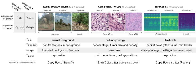
Figure 1: We model inputs as $x=f(x_{\mathsf{obj}},x_{\mathsf{d:robust}},x_{\mathsf{d:spu}},x_{\mathsf{noise}})$, where each of the four types of features are either (i) dependent on the domain $d$ or not and (ii) dependent on the output label $y$ or not, both in the population $P$. We study targeted augmentations, which randomize $x_{\mathsf{d:spu}}$ but preserve $x_{\mathsf{d:robust}}$, and we consider three real-world datasets (Beery et al., 2021; Bandi et al., 2018; Koh et al., 2021), each of which have both robust and spurious domain-dependent features.

2 Problem setting

Domain generalization.  In domain generalization, our goal is to generalize to domains unseen during training. In particular, we seek a model $\theta\in\Theta$ that minimizes the risk under a distribution $P$, where

$$R^{\mathsf{OOD}}(\theta)\triangleq\mathbb{E}_{P}[\ell(\theta;(x,y))],$$ (1)

and $P$ comprises data from all possible domains $\mathcal{D}^{\mathsf{all}}$:

$$P(x,y)=\sum_{d\in\mathcal{D}^{\mathsf{all}}}P(x,y\mid d)P(d),$$ (2)

where we assume $\mathcal{D}^{\mathsf{all}}$ is countable to keep notation simple. To obtain training domains $\mathcal{D}^{\mathsf{train}}\subseteq\mathcal{D}^{\mathsf{all}}$, we sample $D$ domains without replacement from $P(d)$. This yields the training distribution comprising $\mathcal{D}^{\mathsf{train}}$,

$$P^{\mathsf{train}}(x,y)=\sum_{d\in\mathcal{D}^{\mathsf{train}}}P(x,y\mid d)P^{\mathsf{train}}(d),$$ (3)

where $P^{\mathsf{train}}(d)$ is the probability of drawing domain $d$ from the training domains $\mathcal{D}^{\mathsf{train}}$ at training time. The challenge is to generalize from the sampled training domains $\mathcal{D}^{\mathsf{train}}$ to all possible domains $\mathcal{D}^{\mathsf{all}}$ that make up the underlying domain distribution. In real-world experiments and simulations, we estimate OOD performance by evaluating on held-out domains $\mathcal{D}^{\mathsf{test}}$, where $\mathcal{D}^{\mathsf{test}}\cap\mathcal{D}^{\mathsf{train}}=\emptyset$.

Feature decomposition.  In many real-world shifts, such as those in Section 2.1, domain-dependent features contain predictive information that generalizes across all domains. To capture such settings, we introduce the feature decomposition $x=f(x_{\mathsf{obj}},x_{\mathsf{noise}},x_{\mathsf{d:robust}},x_{\mathsf{d:spu}})$ for some complex function $f(\cdot)$ (Figure 1 left). $x$ lies in pixel space, while the features live in some abstract feature space. We split these features along two axes: whether they are robust (i.e., predictive out-of-domain), and whether they are domain dependent (i.e., varying across domains). We formalize these two criteria by (in)dependence with label $y$ and domain $d$, respectively, in the population $P$:

$$x_{\mathsf{obj}},x_{\mathsf{d:robust}}\centernot{\perp\!\!\!\perp}y$$ (4)

$$x_{\mathsf{noise}},x_{\mathsf{d:spu}}\perp\!\!\!\perp y$$

$$x_{\mathsf{d:robust}},x_{\mathsf{d:spu}}\centernot{\perp\!\!\!\perp}d$$

$$x_{\mathsf{obj}},x_{\mathsf{noise}}\perp\!\!\!\perp d$$ .

For example, $y$ depends on robust features $x_{\mathsf{obj}}$ and $x_{\mathsf{d:robust}}$, but is independent of non-robust features $x_{\mathsf{noise}}$ and $x_{\mathsf{d:spu}}$, which yields $P(y\mid x)=P(y\mid x_{\mathsf{obj}},x_{\mathsf{d:robust}})$. Note that prior work typically only considers domain-invariant $x_{\mathsf{obj}}$ relevant for $y$; however, domain-dependent $x_{\mathsf{d:robust}}$ is also useful.

We note that the independencies above need not hold in the training distribution $P^{\mathsf{train}}$ due to finite-domain effects. Recall that $P^{\mathsf{train}}$ is a mixture of $D$ domains. While $x_{\mathsf{d:spu}}\perp\!\!\!\perp y$ in $P$, when $D$ is small, some $x_{\mathsf{d:spu}}$ may be correlated with $y$ in $P^{\mathsf{train}}$. This leads models to learn such features and generalize poorly out-of-domain.

2.1 Real-world datasets

We study three real-world datasets (Figure 1 right), which have both robust and spurious domain-dependent features.

Species classification from camera trap images (iWildCam2020-WILDS).  In iWildCam (Beery et al., 2021; Koh et al., 2021), the task is to classify an animal species $y$ from an image $x$ captured by a static camera trap $d$. There are 243 cameras in $\mathcal{D}^{\mathsf{train}}$. Images from the same camera share nearly identical backgrounds. While low-level details of each domain’s background are generally spurious (e.g., whether there are two trees or three), backgrounds also contain habitat features $x_{\mathsf{d:robust}}$, which are predictive across domains. For example, in Figure 1, cameras 23 and 97 are installed in dry Kenyan savannas, while camera 54 observes a leafy Guatemalan forest. The two regions have different label distributions: in practice, wild African elephants are very unlikely to set foot in Guatemala. Further, habitat features are often necessary for prediction; foregrounds are often blurry or occluded (see Figure 8), so randomizing all domain-dependent features discards useful information.

Tumor identification in histopathology slides (Camelyon17-WILDS).  In Camelyon17 (Bandi et al., 2018; Koh et al., 2021), the task is to classify whether a patch of a histopathology slide contains a tumor. Slides are contributed by hospitals $d$. Variations in imaging technique result in domain-specific stain colorings, which spuriously correlate with $y$ in the training set (see Figure 6). Domains also vary in distributions of patient cancer stage. In Camelyon17’s 3 training hospitals, most patients in Hospitals 1 and 2 have earlier-stage pN1 breast cancer, whereas nearly half of the patients in Hospital 3 have later-stage pN2 stage cancer. The pN stage relates to the size and number of lymph node metastases, which is correlated with other histological tumor features. These useful tumor features thus depend on both $d$ and $y$.

Bird species recognition from audio recordings (BirdCalls).  To monitor bird populations, ornithologists use machine learning to identify birds by their calls in audio recordings. However, generalizing to recordings from new microphones can be challenging (Joly et al., 2021). We introduce a new bird recognition dataset curated from publicly released data (see Appendix A.3 for details). The task is to identify the bird species $y$ vocalizing in audio clip $x$ recorded by microphone $d$. There are 9 microphones in $\mathcal{D}^{\mathsf{train}}$, which vary in their model and location. While low-level noise and microphone settings (e.g., gain levels) only spuriously correlate with $y$, other background noises indicate habitat, like particular insect calls in the Amazon Basin that are absent from other regions (Figure 1). As in iWildCam, these habitat indicators reliably predict $y$. We train models on mel-spectrograms of audio clips.

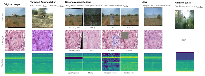
Figure 2: Augmentation examples for the three real-world datasets, including targeted augmentations Copy-Paste (Same Y) for iWildCam, Stain Color Jitter for Camelyon17, and Copy-Paste + Jitter (Region) for BirdCalls. Targeted augmentations randomize $x_{\mathsf{d:spu}}$ but preserve $x_{\mathsf{d:robust}}$. In Section 5.1, we compare to modified Copy-Paste augmentations in the ablation column.

3 Data augmentation

Augmentation types.  We use the feature decomposition from Section 2 to model three types of data augmentations. Generic augmentations designed for in-domain settings often do not randomize domain-dependent features. For example, horizontal flips modify object orientation; this feature varies across examples but is typically distributed similarly across domains. We model generic augmentations as varying $x_{\mathsf{noise}}$, which is label- and domain-independent:

$$A_{\mathsf{gen}}(x)=f(x_{\mathsf{obj}},x_{\mathsf{noise}}^{\prime},x_{\mathsf{d:robust}},x_{\mathsf{d:spu}}),$$ (5)

where $x_{\mathsf{noise}}^{\prime}$ is drawn from some augmentation distribution. Domain-invariant augmentations $A_{\mathsf{inv}}$ aim to randomize all domain-dependent features $x_{\mathsf{d:robust}}$ and $x_{\mathsf{d:spu}}$:

$$A_{\mathsf{inv}}(x)=f(x_{\mathsf{obj}},x_{\mathsf{noise}},x_{\mathsf{d:robust}}^{\prime},x_{\mathsf{d:spu}}^{\prime}),$$ (6)

where $x_{\mathsf{d:robust}}^{\prime},x_{\mathsf{d:spu}}^{\prime}$ are drawn from some distribution. Finally, targeted augmentations $A_{\mathsf{tgt}}$ preserve $x_{\mathsf{d:robust}}$ while aiming to randomize $x_{\mathsf{d:spu}}$:

$$A_{\mathsf{tgt}}(x)=f(x_{\mathsf{obj}},x_{\mathsf{noise}},x_{\mathsf{d:robust}},x_{\mathsf{d:spu}}^{\prime}),$$ (7)

where $x_{\mathsf{d:spu}}^{\prime}$ is drawn from some distribution. Applying generic, domain-invariant, and targeted augmentations to the training distribution $P^{\mathsf{train}}$ yields new distributions over examples $P^{\mathsf{train}}_{\mathsf{gen}},P^{\mathsf{train}}_{\mathsf{inv}},$ and $P^{\mathsf{train}}_{\mathsf{tgt}}$, respectively.

Training.  Given $N$ training examples $\{(x^{(i)},y^{(i)})\}_{i=1}^{N}$ drawn from $P^{\mathsf{train}}$, we learn a model that minimizes the average loss on the (augmented) training data:

$$\hat{\theta}^{\mathsf{(unaug)}}=\operatorname*{arg\,min}_{\theta}\mathbb{E}_{\hat{P}^{\mathsf{train}}}\left[\ell(\theta;(x,y))\right]$$ (8)

$$\hat{\theta}^{\mathsf{(aug)}}=\operatorname*{arg\,min}_{\theta}\mathbb{E}_{\hat{P}^{\mathsf{train}}_{\mathsf{aug}}}\left[\ell(\theta;(x,y))\right],$$ (9)

where $\hat{P}^{\mathsf{train}}$ and $\hat{P}^{\mathsf{train}}_{\mathsf{aug}}$ are the empirical distributions over the unaugmented and augmented training data, respectively. The superscript $\mathsf{aug}$ can stand for $\mathsf{gen}$, $\mathsf{inv}$, or $\mathsf{tgt}$.

3.1 Targeted augmentations for real-world datasets

We instantiate targeted augmentations on real-world datasets from Section 2.1, using domain knowledge about implicit $x_{\mathsf{d:robust}}$ and $x_{\mathsf{d:spu}}$ features. Full details are in Appendix B.

Species classification from camera trap images (iWildCam2020-WILDS).  In iWildCam, image backgrounds are domain-dependent features with both spurious and robust components. While low-level background features are spurious, habitat features are robust. Copy-Paste (Same Y) transforms input $(x,y)$ by pasting the animal foreground onto a random training set background—but only onto backgrounds from training cameras that also observe $y$ (Figure 2). This randomizes low-level background features while roughly preserving habitat. We use segmentation masks from Beery et al. (2021).

Tumor identification in histopathology slides (Camelyon17-WILDS).  In Camelyon17, stain color is a spurious domain-dependent feature, while stage-related features are robust domain-dependent features. Stain Color Jitter (Tellez et al., 2018) transforms $x$ by jittering its color in the hematoxylin and eosin staining color space (Figure 2). In contrast, domain-invariant augmentations can distort cell morphology to attain invariance, which loses information.

Bird species recognition from audio recordings (BirdCalls).  In BirdCalls, low-level noise and gain levels are spurious domain-dependent features, while habitat-specific noise is a robust domain-dependent feature. Copy-Paste + Jitter (Region) leverages time-frequency bounding boxes to paste bird calls onto other training set recordings from the same geographic region (Southwestern Amazon Basin, Hawaii, or Northeastern United States) (Figure 2). After pasting the bird call, we also jitter hue levels of the spectrogram to simulate randomizing microphone gain settings.

4 Analysis and simulations

We now motivate targeted augmentations and illustrate the shortcomings of generic and domain-invariant augmentations in a simple linear regression setting, building off of the framework in Section 2. To our knowledge, our analysis is the first to characterize how different augmentation strategies affect OOD risk and its scaling with the number of domains. It also proposes a natural theoretical setting for OOD generalization, in which the distribution shift arises from finite-domain effects, departing from prior work that considers worst-case shifts (Rosenfeld et al., 2020; Chen et al., 2021b).

4.1 Linear regression setting

Data distribution.  We model each domain $d$ as having latent attributes $\mu^{\scalebox{0.7}{(d)}}\triangleq[\mu_{\mathsf{robust}}^{\scalebox{0.7}{(d)}},\mu_{\mathsf{spu}}^{\scalebox{0.7}{(d)}}]$, which affect the distribution of the corresponding domain-dependent features $x_{\mathsf{d:robust}},x_{\mathsf{d:spu}}$. In iWildCam, $\mu_{\mathsf{robust}}^{\scalebox{0.7}{(d)}}$ intuitively corresponds to a habitat indicator and label prior. In the linear setting, these domain attributes are drawn as

$$\mu_{\mathsf{robust}}^{\scalebox{0.7}{(d)}}\sim\mathcal{N}(0,\tau^{2}I)$$ (10)

$$\mu_{\mathsf{spu}}^{\scalebox{0.7}{(d)}}\sim\mathcal{N}(0,\tau^{2}I)$$ .

The dimensionality of $\mu^{\scalebox{0.7}{(d)}}$ is $p_{\mathsf{dom}}$, and the dimensionality of $\mu_{\mathsf{robust}}^{\scalebox{0.7}{(d)}}$ is $p_{\mathsf{robust}}$. Following the feature decomposition in Figure 1, we consider inputs $x=[x_{\mathsf{obj}},x_{\mathsf{noise}},x_{\mathsf{d:robust}},x_{\mathsf{d:spu}}]$, i.e., $f(\cdot)$ is a concatenation. The training data is drawn uniformly from $D$ training domains. Within each domain, inputs $x$ are drawn according to the following distribution:

$$x_{\mathsf{obj}}\sim\mathcal{N}(0,I)$$ (11)

$$x_{\mathsf{noise}}\sim\mathcal{N}(0,I)$$

$$x_{\mathsf{d:robust}}\mid d\sim\mathcal{N}(\mu_{\mathsf{robust}}^{\scalebox{0.7}{(d)}},\sigma^{2}I)$$

$$x_{\mathsf{d:spu}}\mid d\sim\mathcal{N}(\mu_{\mathsf{spu}}^{\scalebox{0.7}{(d)}},\sigma^{2}I)$$ .

The domain-dependent features $x_{\mathsf{d:robust}}$ and $x_{\mathsf{d:spu}}$ are centered around the corresponding domain attributes $\mu_{\mathsf{robust}}^{\scalebox{0.7}{(d)}}$ and $\mu_{\mathsf{spu}}^{\scalebox{0.7}{(d)}}$, while the domain-independent features $x_{\mathsf{obj}}$ and $x_{\mathsf{noise}}$ are not. We define the variance ratio $\gamma^{2}\triangleq\tau^{2}/\sigma^{2}$, which is the ratio of variances in $\mu^{\scalebox{0.7}{(d)}}$ and feature noise. When $\gamma^{2}>1$, examples within a domain tend to be more similar to each other than to examples from other domains; we consider the typical setting in which $\gamma^{2}>1$.

The output $y\in\mathbb{R}$ is a linear function of both $x_{\mathsf{obj}}$ and robust domain attribute $\mu_{\mathsf{robust}}^{\scalebox{0.7}{(d)}}$:

$$y=\beta_{\mathsf{obj}}^{\top}x_{\mathsf{obj}}+\beta_{\mathsf{robust}}^{\top}\mu_{\mathsf{robust}}^{\scalebox{0.7}{(d)}}+\mathcal{N}(0,\sigma_{\varepsilon}^{2}).$$ (12)

For convenience, we define the parameters for domain-dependent components as $\beta_{\mathsf{dom}}\triangleq[\beta_{\mathsf{robust}},\beta_{\mathsf{spu}}]$ where $\beta_{\mathsf{spu}}=0$. Although $y$ depends on the domain attributes $\mu^{\scalebox{0.7}{(d)}}$, models cannot directly observe $\mu^{\scalebox{0.7}{(d)}}$, and instead only observe the noised features $x_{\mathsf{d:robust}},x_{\mathsf{d:spu}}$.

The data generating process above tells us that in $P$ (2), $y$ and $x_{\mathsf{d:spu}}$ are independent, as $\mu_{\mathsf{robust}}^{\scalebox{0.7}{(d)}}$ and $\mu_{\mathsf{spu}}^{\scalebox{0.7}{(d)}}$ are independent in distribution (10). However, the training distribution $P^{\mathsf{train}}$ is generated from only a small, finite sample of $(\mu_{\mathsf{robust}}^{\scalebox{0.7}{(d)}},\mu_{\mathsf{spu}}^{\scalebox{0.7}{(d)}})$ pairs, one for each of the $D$ training domains. The smaller $D$ is, the more correlated $x_{\mathsf{d:spu}}$ appears with $x_{\mathsf{d:robust}}$ (and thus $y$) in the training distribution. This is true even with infinite examples per domain: so long as $D$ is fixed, more training examples reveal that $x_{\mathsf{d:robust}}\perp\!\!\!\perp x_{\mathsf{noise}}$, but $x_{\mathsf{d:robust}}$ will remain correlated with $x_{\mathsf{d:spu}}$. This finite-domain effect enables models to infer $\mu_{\mathsf{robust}}^{\scalebox{0.7}{(d)}}$ (and thus $y$) not only from $x_{\mathsf{d:robust}}$, but also from $x_{\mathsf{d:spu}}$. Intuitively, models do this by memorizing $(\mu_{\mathsf{robust}}^{\scalebox{0.7}{(d)}},\mu_{\mathsf{spu}}^{\scalebox{0.7}{(d)}})$ pairs inferred from $(x_{\mathsf{d:robust}},x_{\mathsf{d:spu}})$ associations in the training distribution. However, this strategy does not generalize OOD, since in $P$, $x_{\mathsf{d:spu}}$ is independent of $\mu_{\mathsf{robust}}^{\scalebox{0.7}{(d)}}$.

Augmentations.  Recall from Section 3 that generic, domain-invariant, and targeted augmentations replace components of $x$ with draws from an augmentation distribution. We preserve $y$ when augmenting and fix the augmentation distributions to preserve each feature’s marginal distribution:

$$x_{\mathsf{noise}}^{\prime}\sim\mathcal{N}(0,I)$$ (13)

$$x_{\mathsf{d:robust}}^{\prime}\sim\mathcal{N}(0,(\sigma^{2}+\tau^{2})I)$$

$$x_{\mathsf{d:spu}}^{\prime}\sim\mathcal{N}(0,(\sigma^{2}+\tau^{2})I).$$

Models.  We study linear models, specifically ordinary least squares in theoretical analysis (Section 4.2) and ridge regression in simulations (Section 4.3).

4.2 Theory

In this section, we first show that unaugmented models fail to generalize OOD when the domain generalization problem is underspecified (Theorem 1), i.e., when there are fewer training domains than the dimensionality of the domain-dependent features, as is typically the case in real-world domain generalization problems. This motivates targeted augmentations; by eliminating spurious domain-dependent features, targeted augmentations bring the problem to a fully specified regime. We prove that targeted augmentations improve OOD risk in expectation (Theorems 2 and 3), whereas generic and domain-invariant augmentations incur high OOD risk (Corollary 1 and Theorem 4).

Our analysis assumes infinite data per domain, but finite training domains. This allows us to focus on the effects of OOD generalization while simplifying traditional sample complexity issues, which are better understood.

Overview.  We study the expected excess OOD risk $\mathbb{E}\left[R^{\mathsf{OOD}}(\theta)-R^{\mathsf{OOD}}({\theta^{*}})\right]$, where the expectation is over random draws of training domains, and ${\theta^{*}}\triangleq\operatorname*{arg\,min}_{\theta}R^{\mathsf{OOD}}(\theta)$ is the oracle model that attains optimal performance in the population $P$. To show that targeted augmentations improve the expected OOD risk, we lower bound the expected excess risk for unaugmented models, upper bound it for models with targeted augmentations, and then demonstrate a gap between the two bounds. Proofs are in Appendix C.

Lower bound for excess OOD risk with no or generic augmentations.  When the number of domains is smaller than the dimensionality of the domain-dependent features ($D<p_{\mathsf{dom}}$), unaugmented models perform poorly OOD.

Theorem 1 (Excess OOD risk without augmentations).

If $D<p_{\mathsf{dom}}$, the expected excess OOD risk of the unaugmented model is bounded below as

Proof sketch..

The learned estimator has weights $\hat{\theta}^{\mathsf{(unaug)}}_{\mathsf{dom}}=(\sigma^{2}I+M)^{-1}M\beta_{\mathsf{dom}}$, where $M\triangleq\frac{1}{D}\sum_{d=1}^{D}\mu^{\scalebox{0.7}{(d)}}\mu^{\scalebox{0.7}{(d)}\top}$ is a random $p_{\mathsf{dom}}$-dimensional Wishart matrix. As we only observe $D<p_{\mathsf{dom}}$ training domains, $M$ is not full rank, with nullity $p_{\mathsf{dom}}-D$. We lower bound the overall excess risk by the excess risk incurred in the null space of $M$, which is $\frac{\tau^{2}\gamma^{2}}{1+\gamma^{2}}\sum_{i=1}^{p_{\mathsf{dom}}-D}(u_{i}^{\top}\beta_{\mathsf{dom}})^{2}$; each $u_{i}$ is an eigenvector with a zero eigenvalue and the summation term is thus the squared norm of a projection of $\beta_{\mathsf{dom}}$ onto the null space of $M$. In expectation, the squared norm is $||\beta_{\mathsf{dom}}||^{2}(1-\frac{D}{p_{\mathsf{dom}}})$ because $M$ has spherically symmetric eigenvectors. Finally, $\|\beta_{\mathsf{dom}}\|=\|\beta_{\mathsf{robust}}\|$ because $\beta_{\mathsf{spu}}=0$. ∎

To contextualize the bound, we discuss the relative scale of the excess OOD risk with respect to the OOD risk of the oracle model $R^{\mathsf{OOD}}({\theta^{*}})=\sigma_{\varepsilon}^{2}+\tau^{2}\|\beta_{\mathsf{robust}}\|^{2}/(1+\gamma^{2})$, where the first and second terms are from irreducible error in $y$ and feature noise in $x_{\mathsf{d:robust}}$, respectively (Proposition 8). The excess error of the unaugmented model is higher than the second term by a factor of $\gamma^{2}(1-D/p_{\mathsf{dom}}),$ where $\gamma^{2}>1$ is the variance ratio and $D$ is the number of domains. Thus, in typical settings where $D$ is small relative to $p_{\mathsf{dom}}$ and the variance ratio $\gamma^{2}$ is large, unaugmented models suffer substantial OOD error.

Models trained with generic augmentations have the same lower bound (Corollary 1 in Appendix C.4), as applying generic augmentations results in the same model as unaugmented training in the infinite data setting. Our analysis captures the shortcomings of generic augmentations, which primarily improve sample complexity (not domain complexity); as evident in the high OOD risk even in the infinite data setting, improving sample complexity alone fails to achieve OOD robustness.

Motivating targeted augmentations.  The core problem above is underspecification, in which the number of domains is smaller than the dimensionality of the domain-dependent features ($D<p_{\mathsf{dom}}$); there are fewer instances of $\mu^{\scalebox{0.7}{(d)}}$ than its dimensionality (although $\mathbb{E}[xx^{\top}]$ is full rank due to feature noise). In such regimes, it is not possible to approximate $\beta_{\mathsf{dom}}$ well, and models incur high OOD risk. We can mitigate this via targeted augmentations, which randomizes the spurious domain-dependent feature. This decreases the effective dimensionality from $p_{\mathsf{dom}}$ to $p_{\mathsf{robust}}$, the dimensionality of only the robust components, as models would no longer use the spurious feature.

Upper bound for excess OOD risk with targeted augmentations.  With targeted augmentations, the problem (even without feature noise) is no longer underspecified when the number of training domains $D$ is large enough relative to $p_{\mathsf{robust}}<p_{\mathsf{dom}}$. In this fully specified regime, we can upper bound the expected excess OOD risk as $O(\log D/D)$. This resembles the standard rates for random design linear regression up to a log factor (Hsu et al., 2011; Györfi et al., 2002); standard analysis shows that excess ID risk has a $O(1/N)$ convergence rate where $N$ is the number of samples, and we show that excess OOD risk has an analogous convergence rate as a function of the number of domains instead of examples.

Theorem 2 (Excess OOD risk with targeted augmentations).

Assume $\gamma^{2}>1$. For any $0<r<1$ and large enough $D$ such that $D>2(p_{\mathsf{robust}}+2)\log(4Dp_{\mathsf{robust}})/(1-r)^{2}$, the excess OOD risk is bounded above as

$$\mathbb{E}\left[R^{\mathsf{OOD}}(\hat{\theta}^{\mathsf{(tgt)}})-R^{\mathsf{OOD}}({\theta^{*}})\right]$$

$$\leq\frac{\tau^{2}\gamma^{2}\left\|\beta_{\mathsf{robust}}\right\|^{2}}{1+\gamma^{2}}\left(\frac{1}{D}+\frac{2\log(4Dp_{\mathsf{robust}})(p_{\mathsf{robust}}+2)}{D(1+\gamma^{2}r)^{2}}\right).$$

Proof sketch..

The learned estimator has weights $\hat{\theta}^{\mathsf{(tgt)}}_{\mathsf{spu}}=0$ and $\hat{\theta}^{\mathsf{(tgt)}}_{\mathsf{robust}}=(\sigma^{2}I+M_{\mathsf{robust}})^{-1}M_{\mathsf{robust}}\beta_{\mathsf{robust}}$, where $M_{\mathsf{robust}}\triangleq\frac{1}{D}\sum_{d=1}^{D}\mu_{\mathsf{robust}}^{\scalebox{0.7}{(d)}}\mu_{\mathsf{robust}}^{\scalebox{0.7}{(d)}\top}$ is a random $p_{\mathsf{robust}}$-dimensional Wishart matrix. The excess risk can be written as $\sum_{i=1}^{p_{\mathsf{robust}}}\frac{\sigma^{4}(\tau^{2}-\lambda_{i})^{2}}{(\sigma^{2}+\tau^{2})(\lambda_{i}+\sigma^{2})^{2}}(u_{i}^{\top}\beta_{\mathsf{robust}})^{2}$, where $\lambda_{i}$ and $u_{i}$ are eigenvalues and eigenvectors of $M_{\mathsf{robust}}$, respectively. Note that this excess risk is low when $D$ is sufficiently large relative to $p_{\mathsf{robust}}$ such that the eigenvalues are sufficiently close to their expected value $\tau^{2}$. We upper bound the excess OOD risk by applying concentration of measure arguments from Zhu (2012) to the eigenvalues of $M_{\mathsf{robust}}$. ∎

Compared to the lower bound for unaugmented models (Theorem 1), this upper bound has qualitatively different behavior. It depends on $p_{\mathsf{robust}}$ instead of $p_{\mathsf{dom}}$, and it converges to 0 at a fast rate of $O(\log D/D)$ whereas the lowerbound is a negative linear function of the number of $D$.

Targeted augmentations improve expected OOD risk.  We now combine the lower and upper bounds to show that targeted augmentations improve expected OOD risk.

Theorem 3 (Targeted augmentations improve OOD risk).

If $\gamma^{2}>1$ and $p_{\mathsf{robust}}$ is small relative to $p_{\mathsf{dom}}$ such that

$$p_{\mathsf{robust}}<\frac{p_{\mathsf{dom}}}{\log(2p_{\mathsf{dom}})}\cdot\frac{1}{4(1+\gamma^{4}/(\gamma^{2}-1)^{2})},$$

then for $D$ such that

$$D >\frac{4\gamma^{4}}{(\gamma^{2}-1)^{2}}(p_{\mathsf{robust}}+2)\log(2p_{\mathsf{dom}})$$

$$D <p_{\mathsf{dom}}-4(p_{\mathsf{robust}}+2)\log(2p_{\mathsf{dom}}),$$

the improvement in expected OOD risk is positive:

$$\mathbb{E} \left[R^{\mathsf{OOD}}(\hat{\theta}^{\mathsf{(unaug)}})-R^{\mathsf{OOD}}(\hat{\theta}^{\mathsf{(tgt)}})\right]>0.$$

As expected, the minimum and maximum number of domains for which there is a provable gap is proportional to $p_{\mathsf{robust}}$ and $p_{\mathsf{dom}}$, respectively. However, there is some looseness in the bound; in simulations (Section 4.3), we see a substantial gap consistent with the above result, including for $D$ outside the proven range.

Domain-invariant augmentations incur high OOD error.  Finally, we show that domain-invariant augmentations incur high OOD risk in expectation.

Theorem 4 (OOD error with domain-invariant augmentations).

For all $D$, expected OOD risk is

$$\mathbb{E}[R^{\mathsf{OOD}}(\hat{\theta}^{\mathsf{(inv)}})-R^{\mathsf{OOD}}({\theta^{*}})]=\frac{\tau^{2}\gamma^{2}\|\beta_{\mathsf{robust}}\|^{2}}{1+\gamma^{2}}.$$

Because domain-invariant augmentations randomize all domain-dependent features, models do not use any domain-dependent features, including the robust components that are crucial for prediction. As a result, the expected OOD risk is high (higher than the lower bound for unaugmented models in Theorem 1), and the error does not decay with the number of domains $D$.

4.3 Simulations

The analysis in Section 4.2 assumes infinite data per domain. We now present simulation results with finite data in a high-sample ($N=$100\,000$$) and low-sample ($N=$5000$$) regime, where $N$ is the total number of examples across all domains. We fix $\gamma^{2}=10,p_{\mathsf{robust}}=5$ and $p_{\mathsf{spu}}=500$. Additional details and results are in Appendix D.

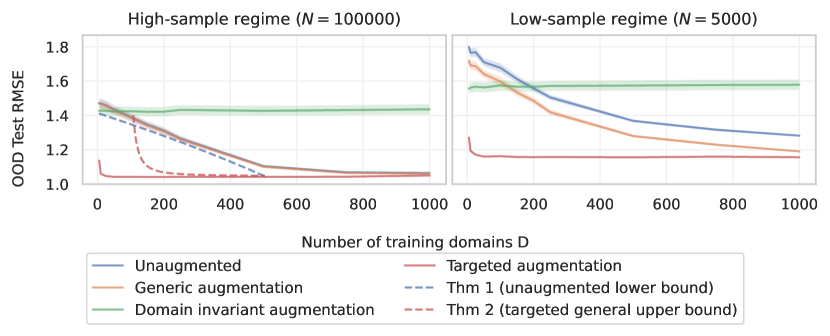
Figure 3: Targeted augmentations (red line) improve OOD error substantially, while generic (orange) or unaugmented (blue) models require many training domains to attain low OOD error. Domain-invariant augmentations (green line) have constant high error. We plot OOD RMSE for varying number of training domains, with standard errors over 10 random seeds. We also plot the risk bounds from Section 4.2 for the high-sample regime; because the bounds assume infinite data, we do not plot them for the low-sample case. The plotted Theorem 2 bound is a more general version (Appendix C.5).

High-sample regime ($N=$100\,000$$).  In Figure 3 (left), we plot OOD RMSE against the number of training domains $D$, together with our upper bound for targeted augmentations (a more general version of Theorem 2 in Appendix C) and lower bound for unaugmented training (Theorem 1).

We observe the trends suggested by our theory. When $D$ is small, the unaugmented model (blue) has high OOD error, and as $D$ increases, OOD error slowly decays. Training with generic augmentation (orange) does not improve over unaugmented training. In contrast, training with targeted augmentation (red) significantly reduces OOD error. There is a substantial gap between the red and orange/blue lines, which persists even when $D$ is outside of the window guaranteed by Theorem 3. Finally, domain-invariant augmentations result in high OOD error (green) that does not decrease with increasing domains, as in Theorem 4.

Low-sample regime ($N=$5000$$).  In Figure 3 (right), we plot OOD RMSE against the number of training domains $D$ when the sample size is small. The unaugmented and targeted models follow the same trends as in the high-sample regime. However, in the low-sample regime, generic augmentation does reduce OOD error compared to the unaugmented model. When the total number of examples $N$ is small, models are incentivized to memorize individual examples using $x_{\mathsf{noise}}$. Generic augmentation prevents this behavior, resulting in an ID and OOD improvement over unaugmented training (also see Figure 11 in Appendix D). However, the OOD error of generic augmentation only decays slowly with $D$ and is significantly higher than targeted augmentation for $D<$1000$$. Domain-invariant augmentation results in a constant level of OOD error, which improves over the unaugmented and generic models for small values of $D$, but underperforms once $D$ is larger.

Overall, our simulations corroborate the theory and show that targeted augmentations offer significant OOD gains in the linear regression setting. In contrast, generic and domain-invariant augmentations improve over unaugmented training only in the low-sample regime.

5 Experiments on real-world datasets

We return to the real-world datasets (iWildCam2020-WILDS, Camelyon17-WILDS, BirdCalls) and augmentations introduced in Section 2.1, where we compare targeted augmentations to unaugmented training, generic augmentations, and domain invariance baselines. To approximate the overall distribution $P$ (2), we evaluate on held-out domains $\mathcal{D}^{\mathsf{test}}$, where $\mathcal{D}^{\mathsf{test}}\cap\mathcal{D}^{\mathsf{train}}=\emptyset$.

Generic augmentations.  On image datasets iWildCam and Camelyon17, we compare to RandAugment (Cubuk et al., 2020), CutMix (Yun et al., 2019), MixUp (Zhang et al., 2017), and Cutout (DeVries & Taylor, 2017). On audio dataset BirdCalls, we compare to MixUp, SpecAugment (Park et al., 2019), random low / high pass filters, and noise reduction via spectral gating (Sainburg, 2022). Since the targeted augmentation for BirdCalls (Copy-Paste + Jitter (Region)) includes color jitter as a subroutine, we also include a baseline of augmenting with only color jitter.

Domain invariance baselines.  We compare to LISA (Yao et al., 2022), a data augmentation strategy that aims to encourage domain invariance by applying either MixUp or CutMix to inputs of the same class across domains. We also compare to other domain invariance algorithms that do not involve augmentation: (C)DANN (Long et al., 2018; Ganin et al., 2016), DeepCORAL (Sun & Saenko, 2016; Sun et al., 2017), and IRM (Arjovsky et al., 2019).

Samples of the augmentations are shown in Figure 2. Additional experimental details can be found in Appendix E.2. Code and BirdCalls are released at this link.

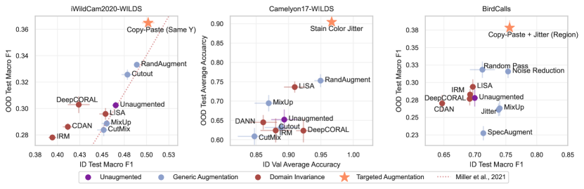
Figure 4: We plot the in-domain (ID) performance of methods against their out-of-domain (OOD) performance. Error bars are standard errors over replicates. Targeted augmentations significantly improve OOD performance over the nearest baseline, improving OOD Macro F1 on iWildCam from 33.3% $\to$ 36.5%, OOD average accuracy on Camelyon17 from 75.3% $\to$ 90.5%, and OOD Macro F1 on BirdCalls from 31.8% $\to$ 37.8%. Tables and additional details can be found in Appendix E.

5.1 Results

Figure 4 plots the average ID versus OOD performance of each method. On all three datasets, targeted augmentations significantly improve OOD performance. Compared to the best-performing baseline, targeted augmentations improve OOD Macro F1 on iWildCam from 33.3% $\to$ 36.5%, OOD average accuracy on Camelyon17 from 75.3% $\to$ 90.5%, and OOD Macro F1 on BirdCalls from 31.8% $\to$ 37.8%. On iWildCam and Camelyon17, which are part of the WILDS benchmark, these targeted augmentations set new state-of-the-art performances (Koh et al., 2021).

Several generic augmentations were also able to improve OOD performance, although by smaller amounts than targeted augmentations; this matches our simulations in the low-sample regime in Section 4.3. RandAugment (Cubuk et al., 2020) performs strongly on iWildCam and Camelyon17, and both noise reduction and random high / low pass filters perform well on BirdCalls. Some generic augmentations degraded performance (MixUp, CutMix, and SpecAugment), which may reflect the fact that these augmentations can also distort $x_{\mathsf{obj}}$ and $x_{\mathsf{d:robust}}$, e.g., by mixing cell morphologies on Camelyon17.

Effective robustness.  On iWildCam, Miller et al. (2021) showed that the ID and OOD performances of models across a range of sizes are linearly correlated; we plot their linear fit on Figure 4 (left). We found that our targeted augmentation Copy-Paste (Same Y) confers what Miller et al. (2021) termed effective robustness, which is represented in the plot by a vertical offset from the line. In contrast, generic augmentations improve OOD performance along the plotted line. While the domain invariance methods also show effective robustness, they mostly underperform the unaugmented model in raw performance numbers.

Although neither Camelyon17 nor BirdCalls have associated linear fits, we observe similar trends in Figure 4, with targeted augmentations offering significant OOD gains even at similar ID performances as other methods.

Ablation on $x_{\mathsf{d:robust}}$.  To demonstrate the importance of preserving $x_{\mathsf{d:robust}}$, we modified the targeted augmentations for iWildCam and BirdCalls to be non-selective. On iWildCam, Copy-Paste (Same Y) selectively pastes animal foregrounds onto backgrounds from domains which also observe $y$ in the training set; as an ablation, we studied Copy-Paste (All Backgrounds), which draws backgrounds from all training domains, including cameras in which $y$ was not observed. Similarly, on BirdCalls, Copy-Paste + Jitter (Region) only pastes calls onto recordings from the original microphone’s region; as an ablation, we studied Copy-Paste + Jitter (All Regions), which merges recordings indiscriminately. These modified augmentations fail to preserve habitat features $x_{\mathsf{d:robust}}$. In Table 1, we see that preserving $x_{\mathsf{d:robust}}$ is important—compared to their targeted variants, the modified augmentations decrease OOD performance by 1.8% on iWildCam and 4.1% on BirdCalls.

Table 1: Randomizing habitat features in iWildCam2020-WILDS and BirdCalls degrades performance.

Dataset	Method	ID Test Macro F1	OOD Test Macro F1
iWildCam	Unaugmented	46.5 (0.4)	30.2 (0.3)
	Copy-Paste (All Backgrounds)	47.1 (1.1)	34.7 (0.5)
	Copy-Paste (Same Y)	50.2 (0.7)	36.5 (0.4)
BirdCalls	Unaugmented	70.0 (0.5)	27.8 (1.2)
	Copy-Paste + Jitter (All Regions)	76.0 (0.3)	33.7 (1.0)
	Copy-Paste + Jitter (Same Region)	75.6 (0.3)	37.8 (1.0)

Table 2: Finetuning CLIP ViT-L/14 with targeted augmentations improves OOD performance on Camelyon17-WILDS (accuracy) and iWildCam2020-WILDS (macro F1). Results averaged over 5 seeds with standard errors.

Dataset	Method	ID Performance	OOD Performance
Camelyon17	Unaugmented	99.5 (0.0)	96.0 (0.2)
	Stain Color Jitter	99.4 (0.0)	97.1 (0.0)
iWildCam	Unaugmented	55.6 (0.8)	43.5 (0.7)
	Copy-Paste (Same Y)	56.6 (0.7)	45.5 (0.3)

Targeted augmentations improve OOD performance when finetuning CLIP.  We also applied our targeted augmentations to CLIP ViT-L/14 (Radford et al., 2021), a large-scale vision-language model (Table 2). Targeted augmentations offer 1.1% and 2% OOD average gains over unaugmented finetuning on iWildCam and Camelyon17.

6 Related work

Additional related work is found in Appendix F.

Data augmentations for OOD robustness.  Prior work has shown that generic augmentations designed for ID performance can improve OOD performance, but this effect is inconsistent across datasets (Gulrajani & Lopez-Paz, 2020; Hendrycks et al., 2021; Wiles et al., 2021). Other work has sought to design augmentations specifically for robustness; these are often inspired by domain invariance and aim to randomize all domain-dependent features, including robust features $x_{\mathsf{d:robust}}$ (Wang et al., 2020; Xu et al., 2020; Yan et al., 2020; Yao et al., 2022). In contrast, we preserve $x_{\mathsf{d:robust}}$ in targeted augmentations.

Analysis on data augmentations and domain generalization.  Existing work usually analyzes augmentations in the standard i.i.d. setting (Dao et al., 2019; He et al., 2019; Chen et al., 2020; Lyle et al., 2020), where augmentations improve sample complexity and reduce variance. We instead analyze the effect of data augmentation on OOD performance. There is limited theoretical work in this setting: Ilse et al. (2021) use augmentations to simulate interventions on domains, and Wang et al. (2022) show that one can recover a causal model given a set of augmentations encoding the relevant invariances. These works are part of a broader thread of analysis which emphasizes robustness to worst-case domain shifts; the aim is thus to recover models that only rely on causal features. In contrast, we seek to generalize to unseen domains on average. Our analysis is related to work on meta-learning (Chen et al., 2021a; Jose & Simeone, 2021); however, these analyses focus on adaptation to new tasks instead of out-of-domain generalization.

Failures of domain invariance.  To improve OOD robustness, the domain invariance literature focuses on learning models which are invariant to domain-dependent features, such that representations are independent of domain marginally (Ganin et al., 2016; Albuquerque et al., 2019). Several works have pointed out failure modes of this approach, including Mahajan et al. (2021), who focus on cases where the distribution of causal features vary across domains; we additionally allow for $x_{\mathsf{d:robust}}$ to be non-causal, e.g., habitat features in iWildCam and BirdCalls.

7 Conclusion

We studied targeted augmentations, which randomize spurious domain-dependent features while preserving robust ones, and showed that they can significantly improve OOD performance over generic and domain-invariant augmentations. These results illustrate that when the out-of-domain generalization problem is underspecified, prior knowledge can provide additional structure and make the out-of-domain generalization problem more tractable. Future work could also explore methods for learning, rather than hand-designing, targeted augmentations; such approaches could leverage high-level prior knowledge on $x_{\mathsf{d:robust}}$, or directly infer $x_{\mathsf{d:robust}}$ from the training domains.

Appendix A Additional notes on datasets

In this appendix, we provide additional analysis justifying the decomposition of robust and spurious domain-dependent features in the real-world datasets. We also provide details on the construction of BirdCalls.

A.1 iWildCam2020-WILDS

Analysis on domain-dependent features.  Figure 8 depicts a sample of images from the iWildCam training set. This figure illustrates that animal foregrounds—which are often blurry, occluded, or camouflaged – are alone insufficient for prediction. Extracting habitat features from the background gives useful signal on what species (out of 182 classes) are likely for an image. We emphasize that $x_{\mathsf{d:robust}}$ is reliable under realistic distribution shifts for this application: since camera traps monitor wild animals in their natural habitats, adversarial shifts as dramatic as swapping animals between Kenya and Guatemala (Figure 8) are unlikely. Further, we show in Section 5.1 that being too conservative to this adversarial shift can reduce OOD performance on relevant, widespread shifts (across cameras).

A.2 Camelyon17-WILDS

Analysis on domain-dependent features.  Figure 9 depicts a sample of images from the Camelyon17 training set. This figure illustrates that cell morphologies are affected by distributions of patients and their breast cancer stage; Figure 5 concretizes how the distribution of cancer stages varies across domains.

We note that unlike iWildCam2020-WILDS and BirdCalls, domains in Camelyon17-WILDS have the same (class-balanced) label distribution. To understand why models are incentivized to memorize stain color in this task, we plot the class-separated color histograms for the three training domains in Figure 6. We see that, on train, models can learn a threshold function based on the class color means for prediction.

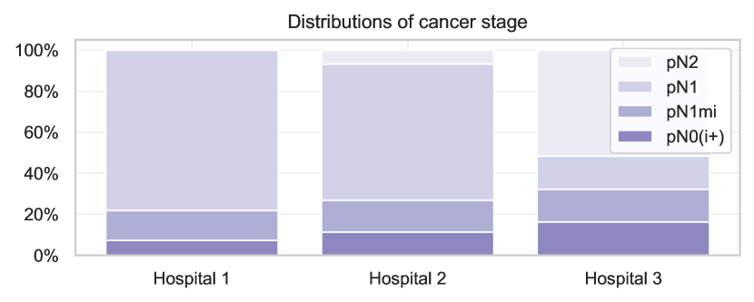
Figure 5: Hospitals vary in the distribution of cancer stages they observe in patients, due to the different patient distributions they service. This in turn affects the causal feature for cancer prediction (cell morphology).

Figure 6: Class-separated color histograms for Camelyon17-WILDS.

A.3 BirdCalls

Problem setting.  To monitor the health of bird populations and their habitats, ornithologists collect petabytes of acoustic recordings from the wild each year. Machine learning can automate analysis of these recordings by learning to recognize species from audio recordings of their vocalizations. However, several features vary across the microphones that collect these recordings, such as microphone model, sampling rate, and recording location. These shifts can degrade model performance on unseen microphones.

Table 3: Test-to-test comparison on BirdCalls

	ID Test Avg Acc	ID Test Macro F1	OOD Test Avg Acc	OOD Test Macro F1
Train on OOD data	16.7 (0.2)	4.1 (0.1)	84.4 (0.7)	51.9 (0.9)
Train on ID data	79.8 (0.4)	70.8 (0.6)	44.6 (0.8)	23.9 (1.0)

Dataset construction and statistics.  To study targeted augmentations for this setting, we curate a bird recognition dataset by combining publicly released datasets. The original data is sourced from 32kHz long recordings from Navine et al. (2022); Hopping et al. (2022); Kahl et al. (2022), which were released alongside expert-annotated time-frequency bounding boxes around observed bird calls. To build our dataset from these long recordings, we extracted all 5-second chunks in which a single (or no) species makes a call, and then we undersampled majority classes to achieve a more balanced class distribution. Our curated dataset, BirdCalls, contains 4,897 audio clips from 12 microphones distributed between the Northeastern United States, Southwest Amazon Basin, and Hawai’i. Each clip features one of 31 bird species, or no bird (we include an extra class for “no bird recorded”). The dataset is split as follows:

1. Train: 2,089 clips from 9 microphones

2. ID Validation: 407 clips from 8 of the 9 microphones in the training set

3. ID Test: 1,677 clips from the 9 microphones in the training set

4. OOD Test: 724 clips from 3 different microphones

To train classification models, we convert the 5-second audio clips into Mel spectrograms and train an EfficientNet-B0 on these images, following prior work (Denton et al., 2022). We evaluate ID and OOD performance on their corresponding test sets. The label distribution of this dataset is shown in Figure 7; to account for remaining class imbalance, we report Macro F1 as the evaluation metric. We show additional samples of the data in Figure 10.

Verifying performance drops.  We ran checks to verify that observed ID to OOD performance drops were due to distribution shift, and not due to having an innately more difficult OOD Test set. For these analyses, we further split the OOD Test set into three temporary splits: OOD Train (365 clips), OOD Validation (69 clips), and OOD Test (290). We then compared the (subsetted) OOD Test performance of models trained on the (ID) Train split + selected on the ID Validation split with models trained on the OOD Train split + selected on the OOD Validation split. The results are shown in Table 3. We see that models perform quite on OOD Test if trained on the same distribution of data (OOD Train). This verifies that the ID to OOD performance drops are due to distribution shift.

Analysis on domain-dependent features.  Figure 10 depicts a sample of images from the BirdCalls training set. This figure shows how habitat features distinctly vary across domains. Since fine-grained bird species are almost disjoint across regions, habitat features help indicate which species are likely. Correspondingly, we show in Section 5.1 that retaining habitat features improve both ID and OOD performance.

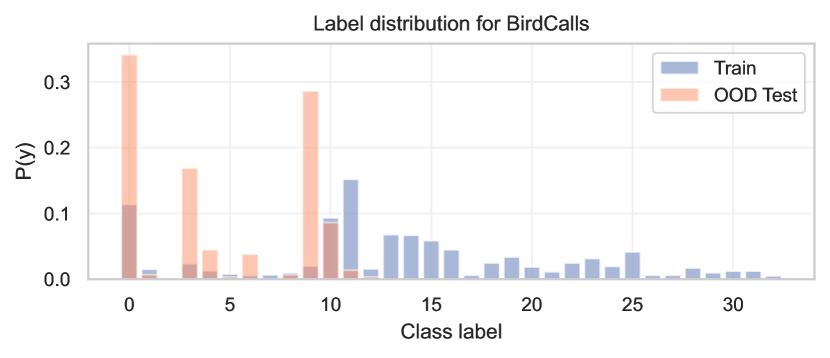
Figure 7: Label distribution of BirdCalls.

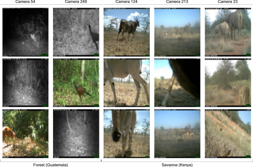
Figure 8: Across domains (columns), both low-level background details $x_{\mathsf{d:spu}}$ and high-level habitat features $x_{\mathsf{d:robust}}$ vary. Since $x_{\mathsf{d:robust}}\not\perp d$, domain invariance may eliminate habitat information. In contrast, a targeted augmentation, Copy-Paste (Same Y), randomizes backgrounds between cameras in similar habitats, preserving the ability of the model to use $x_{\mathsf{d:robust}}$. This is necessary for performance, as foregrounds $x_{\mathsf{obj}}$ can be too camouflaged, distant, blurred, dark, or occluded for even a human annotator’s eye. (All images in this figure contain an animal.)

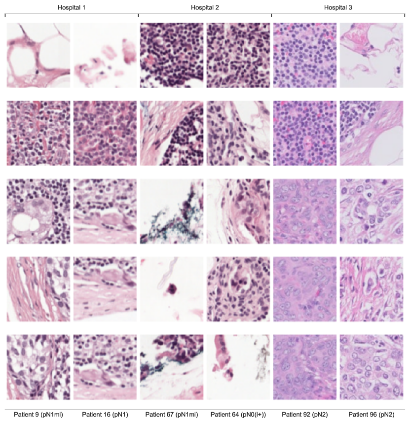
Figure 9: The top two rows depict non-cancerous patches ($y=0$), while the bottom three rows are cancerous patches ($y=1$). Across domains (columns), several features, including distributions of the causal feature (cell morphology), vary. Cell morphology is impacted by the patient distribution of each hospital, as some hospitals have patients with more aggressive cancer staging (Figure 5). This leads to different distributions of cell morphologies across domains. While domain invariance would thus eliminate this causal feature, targeted augmentations only randomize features independent of $y$, such as stain color.

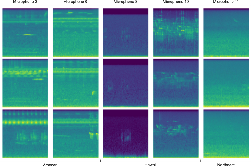
Figure 10: Across domains (columns), recordings vary in their habitat features, such as calls from local insects (left two columns, high frequencies), stronger wind levels (center two columns), or rainfall levels. These habitat features can act as a useful bias for deciding likely labels. Targeted augmentations randomize background noise between microphones located in the same region, preserving this robust feature, while domain invariance eliminates this feature.

Appendix B Augmentation details

In this appendix, we provide implementation details for the targeted augmentations we study on the real-world datasets.

B.1 Copy-Paste (Same Y) on iWildCam2020-WILDS

The full Copy-Paste protocol is given in Algorithm 1. We consider two strategies for selecting the set of valid empty backgrounds $B^{(i)}$.

1. Copy-Paste (All Backgrounds): all empty train split images. $B^{(i)}=\{(x,y,d)\in\mathcal{\mathcal{D}^{\mathsf{train}}}:y=\text{``empty''}\}$, i.e., all augmented examples should have a single distribution of backgrounds. There is a large set of training backgrounds to choose from when executing the procedure – of $129,809$ training images, $48,021$ are empty images.

2. Copy-Paste (Same Y): empty train split images from cameras that have observed $y^{(i)}$. Let $\mathcal{Y}(d)$ represent the set of labels domain $d$ observes. Then $B^{(i)}=\{(x,y,d)\in\mathcal{\mathcal{D}^{\mathsf{train}}}:y=\text{``empty''}\text{ and }y^{(i)}\in\mathcal{Y}(d)\}$.

  Input: Labeled example $(x^{(i)},y^{(i)},d^{(i)})$, binary segmentation mask $m^{(i)}$, set of images to sample empty images from to use as backgrounds $B^{(i)}$

  if $y^{(i)}$ = “empty” or $|B^{(i)}|=0$ then

     Return $x^{(i)}$

  end if

  Copy out foreground by applying segmentation mask $f^{(i)}:=m^{(i)}\circ x^{(i)}$

  Randomly select a background $b\in B^{(i)}$

  Paste $f^{(i)}$ onto $b$ and return $\tilde{x}^{(i)}:=\text{Paste}(f^{(i)},b)$

Algorithm 1 Copy-Paste

Segmentation masks.  The iWildCam dataset is curated from real camera trap data collected by the Wildlife Conservation Society and released by Beery et al. (2021); Koh et al. (2021). Beery et al. (2021) additionally compute and release segmentation masks for all labeled examples in iWildCam. These segmentation masks were extracted by running the dataset through MegaDetector (Beery et al., 2019) and then passing regions within detected boxes through an off-the-shelf, class-agnostic detection model, DeepMAC (Birodkar et al., 2021). We use these segmentation masks for our Copy-Paste augmentation.

Table 4: Pasting onto backgrounds from cameras that have observed the same class during training achieves similar ID and OOD performance to pasting within countries.

	ID Test Macro F1	OOD Test Macro F1
Copy-Paste (Same Y)	50.2 (0.7)	36.5 (0.4)
Copy-Paste (Same Country)	49.3 (0.9)	36.7 (0.7)

Comparison to swapping within countries.  To confirm that Copy-Paste (Same Y) acts to preserve geographic habitat features, we ran an oracle experiment comparing its performance to applying Copy-Paste within geographic regions. Beery et al. (2021) released noisy geocoordinates for around half of the locations in iWildCam2020-WILDS. Using these coordinates, we inferred the country each camera trap was located in (we merged all cameras of unknown locations into one group, “unknown country”). We then applied Copy-Paste, pasting animals only onto backgrounds from the same country. Table 4 shows that Copy-Paste (Same Y) and this oracle have the same performance, suggesting that the Same Y policy indeed preserves geographic habitat features.

B.2 Stain Color Jitter on Camelyon17-WILDS

The full Stain Color Jitter protocol, originally from Tellez et al. (2018), is given in Algorithm 2. The augmentation uses a pre-specified Optical Density (OD) matrix from Ruifrok et al. (2001) to project images from RGB space to a three-channel hematoxylin, eosin, and DAB space before applying a random linear combination.

  Input: Labeled example $(x^{(i)},y^{(i)},d^{(i)})$, normalized OD matrix $M$ (Ruifrok et al., 2001), tolerance $\epsilon=1^{-6}$

  $S=-\log(x^{(i)}+\epsilon)M^{-1}$

  Sample $\alpha\sim\text{Uni}(1-\sigma,1+\sigma)$

  Sample $\beta\sim\text{Uni}(-\sigma,\sigma)$

  $P=\exp[-(\alpha S+\beta)M]-\epsilon$

  Return $P$ with each cell clipped to $[0,255]$

Algorithm 2 Stain Color Jitter Augmentation

B.3 Copy-Paste + Jitter (Region) on BirdCalls

After transforming audio clips into mel-spectrograms, we use time-frequency bounding boxes included in the dataset to extract pixels of bird calls. We then paste these pixels onto spectrograms from the empty (no bird recorded) class, applying Algorithm 1. Finally, we apply color jitter on the spectrograms. The goal of jitter is to simulate changes in gain settings across microphones, which affect the coloring of spectrograms. We consider two strategies for selecting the set of valid empty backgrounds $B^{(i)}$.

1. Copy-Paste + Jitter (All Regions): all empty train split recordings. $B^{(i)}=\{(x,y,d)\in\mathcal{\mathcal{D}^{\mathsf{train}}}:y=\text{``empty''}\}$, i.e., all augmented examples should have a single distribution of backgrounds. There is a large set of training backgrounds to choose from when executing the procedure – of $129,809$ training images, $48,021$ are empty images.

2. Copy-Paste + Jitter (Region): empty train split recordings from microphones in the same region. Let $R(d)$ represent the region (Hawaii, Southwest Amazon Basin, or Northeastern United States) that domain $d$ is located in; we provide these annotations in BirdCalls. Then $B^{(i)}=\{(x,y,d)\in\mathcal{\mathcal{D}^{\mathsf{train}}}:y=\text{``empty''}\text{ and }R(d^{(i)})=R(d)\}$.

Appendix C Proofs

We present the proofs for results presented in Section 4.2.

C.1 Analyzing domain-dependent features only

In the proofs, we analyze only the domain-dependent features $x_{\mathsf{dom}}=[x_{\mathsf{d:robust}},x_{\mathsf{d:spu}}]$, disregarding the object features $x_{\mathsf{obj}}$ and noise features $x_{\mathsf{noise}}$, since the latter two features do not affect our results. To show this, we first consider the full setting with $x=[x_{\mathsf{obj}},x_{\mathsf{noise}},x_{\mathsf{d:robust}},x_{\mathsf{d:spu}}]$ and compute the model estimate $\hat{\theta}$ by applying the normal equations. We compute the relevant quantities as

$$\mathbb{E}[xx^{\top}]=\begin{pmatrix}I&0&0\\ 0&I&0\\ 0&0&A\\ \end{pmatrix},\mathbb{E}[yx]=\begin{pmatrix}\beta_{\mathsf{obj}}\\ \beta_{\mathsf{noise}}\\ B\beta_{\mathsf{dom}}\\ \end{pmatrix},$$ (14)

where the blocks correspond to object features $x_{\mathsf{obj}}$, noise features $x_{\mathsf{noise}}$, and domain-dependent features $[x_{\mathsf{d:robust}},x_{\mathsf{d:spu}}]$ and the matrices $A$ and $B$ depend on the augmentation strategy. Applying the normal equations yields

$$\hat{\theta}=\begin{pmatrix}\beta_{\mathsf{obj}}\\ \beta_{\mathsf{noise}}\\ A^{-1}B\beta_{\mathsf{dom}}.\end{pmatrix}$$ (15)

This means that in our infinite-data, finite-domain setting, models perfectly recover $\beta_{\mathsf{obj}}$ and $\beta_{\mathsf{noise}}$ for all augmentation strategies. Thus, the model incurs zero error from the object and noise dimensions, so these features can also be disregarded in the error computation.

In the rest of the proof, we focus on analyzing the domain-dependent features; without loss of generality, we assume that the dimensionality of the object and noise features are 0. In other words, we consider $x=[x_{\mathsf{d:robust}},x_{\mathsf{d:spu}}]$, $\beta=\beta_{\mathsf{dom}}=[\beta_{\mathsf{robust}},\beta_{\mathsf{spu}}]$, and $\theta=\theta_{\mathsf{dom}}=[\theta_{\mathsf{robust}},\theta_{\mathsf{spu}}]$, all of which are of length $p_{\mathsf{dom}}$.

C.2 Models

Proposition 1 (Estimator without augmentation).

Unaugmented training yields the model

$$\hat{\theta}^{\mathsf{(unaug)}} =(\Sigma+M)^{-1}M\beta$$ (16)

where $M=\frac{1}{D}\sum_{d=1}^{D}\mu^{\scalebox{0.7}{(d)}}\mu^{\scalebox{0.7}{(d)}\top}$ and $\Sigma=\sigma^{2}I$.

Proof.

$$\hat{\theta}^{\mathsf{(unaug)}} =\mathbb{E}[xx^{\top}]^{-1}\mathbb{E}[xy]$$ (17)

$$=\left(\frac{1}{D}\sum_{d=1}^{D}\Sigma+\mu^{\scalebox{0.7}{(d)}}\mu^{\scalebox{0.7}{(d)}\top}\right)^{-1}\left(\frac{1}{D}\sum_{d=1}^{D}\mathbb{E}\left[x(\beta\cdot\mu^{\scalebox{0.7}{(d)}}+\varepsilon)\right]\right)$$ (18)

$$=\left(\Sigma+\frac{1}{D}\sum_{d=1}^{D}\mu^{\scalebox{0.7}{(d)}}\mu^{\scalebox{0.7}{(d)}\top}\right)^{-1}\left(\frac{1}{D}\sum_{d=1}^{D}\mu^{\scalebox{0.7}{(d)}}\mu^{\scalebox{0.7}{(d)}\top}\beta\right)$$ (19)

$$=\left(\Sigma+M\right)^{-1}M\beta$$ (20)

∎

Proposition 2 (Estimator with generic augmentation).

Applying generic augmentation yields the model

$$\hat{\theta}^{\mathsf{(gen)}} =(\Sigma+M)^{-1}M\beta$$ (21)

where $M=\frac{1}{D}\sum_{d=1}^{D}\mu^{\scalebox{0.7}{(d)}}\mu^{\scalebox{0.7}{(d)}\top}$ and $\Sigma=\sigma^{2}I$.

Proof.

Applying generic augmentations do not change the data distribution over the domain-dependent features. Thus, $\hat{\theta}^{\mathsf{(gen)}}=\hat{\theta}^{\mathsf{(unaug)}}$. Applying Proposition 1 yields the result.

∎

Proposition 3 (Estimator with targeted augmentation).

Applying targeted augmentation yields the model

$$\hat{\theta}^{\mathsf{(tgt)}}=\begin{pmatrix}(\Sigma_{\mathsf{robust}}+M_{\mathsf{robust}})^{-1}M_{\mathsf{robust}}\beta_{\mathsf{robust}}\\ 0\end{pmatrix}$$ (22)

where $M_{\mathsf{robust}}=\frac{1}{D}\sum_{d=1}^{D}\mu_{\mathsf{robust}}^{\scalebox{0.7}{(d)}}\mu_{\mathsf{robust}}^{\scalebox{0.7}{(d)}\top}$ and $\Sigma_{\mathsf{robust}}=\sigma^{2}I$.

Proof.

In the augmented training distribution, input $x$ in domain $d$ is distributed as

$$x\sim N\left(\begin{pmatrix}\mu_{\mathsf{robust}}^{\scalebox{0.7}{(d)}}\\ 0\end{pmatrix},\Sigma^{\mathsf{(tgt)}}\right),$$ (23)

where $\Sigma^{\mathsf{(tgt)}}=\begin{pmatrix}\sigma^{2}I&0\\ 0&(\sigma^{2}+\tau^{2})I\end{pmatrix}$.

Applying the normal equations on the augmented training distribution, we compute $\hat{\theta}^{\mathsf{(tgt)}}$ as

$$\hat{\theta}^{\mathsf{(tgt)}} =\mathbb{E}[xx^{\top}]^{-1}\mathbb{E}[xy]$$ (24)

$$=\left(\Sigma^{\mathsf{(tgt)}}+M^{\mathsf{(tgt)}}\right)^{-1}M^{\mathsf{(tgt)}}\beta,$$ (25)

where $M^{\mathsf{(tgt)}}=\begin{pmatrix}M_{\mathsf{robust}}&0\\ 0&0\end{pmatrix}$.

Since we can invert block diagonal matrices block by block, we can compute $\left(\Sigma^{\mathsf{(tgt)}}+M^{\mathsf{(tgt)}}\right)^{-1}$ as

$$\left(\Sigma^{\mathsf{(tgt)}}+M^{\mathsf{(tgt)}}\right)^{-1} =\begin{pmatrix}(\sigma^{2}I+M_{\mathsf{robust}})^{-1}&0\\ 0&\frac{1}{\sigma^{2}+\tau^{2}}I\end{pmatrix}.$$ (26)

As a result of the block structure, we can simplify $\hat{\theta}^{\mathsf{(tgt)}}$ as

$$\hat{\theta}^{\mathsf{(tgt)}}=\begin{pmatrix}(\sigma^{2}I+M_{\mathsf{robust}})^{-1}M_{\mathsf{robust}}\beta_{\mathsf{robust}}\\ 0\end{pmatrix}$$ (27)

∎

Proposition 4 (Estimator with domain-invariant augmentations).

Applying domain-invariant augmentation yields the model

$$\hat{\theta}^{\mathsf{(inv)}}=0.$$ (28)

Proof.

In the augmented training distribution, input $x$ in domain $d$ is distributed as

$$x\sim N\left(0,\Sigma+T\right).$$ (29)

Applying the normal equations thus yields $\hat{\theta}^{\mathsf{(inv)}}=0$. ∎

Proposition 5 (Oracle model).

Recall that ${\theta^{*}}\triangleq\operatorname*{arg\,min}_{\theta}R^{\mathsf{OOD}}(\theta)$ is the oracle model that attains optimal performance in the population $P$. The oracle model is

$${\theta^{*}} =(\Sigma+T)^{-1}T\beta,$$ (30)

where $\Sigma=\sigma^{2}I$ and $T=\tau^{2}I$.

Proof.

As the number of domains $D\rightarrow\infty$, $M$ converges to $T$. Applying the normal equations yields the result. ∎

C.3 Computation of ID and OOD errors

Proposition 6 (OOD error as a function of $\theta$).

The OOD error of a model $\theta$ is

$$R^{\mathsf{OOD}}(\theta)=\sigma_{\varepsilon}^{2}+\theta^{\top}\Sigma\theta+\left(\beta-\theta\right)^{\top}T\left(\beta-\theta\right),$$ (31)

where $\Sigma=\sigma^{2}I$ and $T=\tau^{2}I$.

Proof.

$$R^{\mathsf{OOD}}(\theta)= \mathbb{E}_{x,y,d}\left[\left(y-\theta\cdot x\right)^{2}\right]$$ (32)

$$= \mathbb{E}_{d}\left[\mathbb{E}_{x,y\mid d}\left[\left(y-\theta\cdot x\right)^{2}\right]\right]$$ (33)

$$= \mathbb{E}_{d}\left[\mathbb{E}_{x,y\mid d}\left[\left(\beta_{\mathsf{robust}}\cdot\mu_{\mathsf{robust}}^{\scalebox{0.7}{(d)}}+\varepsilon-\theta\cdot x\right)^{2}\right]\right]$$ (34)

$$= \sigma_{\varepsilon}^{2}+\mathbb{E}_{d}\left[\left(\beta\cdot\mu^{\scalebox{0.7}{(d)}}\right)^{2}+\theta^{\top}\left(\Sigma+\mu^{\scalebox{0.7}{(d)}}\mu^{\scalebox{0.7}{(d)}\top}\right)\theta-2\left(\beta\cdot\mu^{\scalebox{0.7}{(d)}}\right)\left(\theta\cdot\mu^{\scalebox{0.7}{(d)}}\right)\right]$$ (35)

$$= \sigma_{\varepsilon}^{2}+\theta^{\top}\Sigma\theta+\left(\beta-\theta\right)^{\top}\mathbb{E}\left[\mu^{\scalebox{0.7}{(d)}}\mu^{\scalebox{0.7}{(d)}\top}\right]\left(\beta-\theta\right)$$ (36)

$$= \sigma_{\varepsilon}^{2}+\theta^{\top}\Sigma\theta+\left(\beta-\theta\right)^{\top}T\left(\beta-\theta\right)$$ (37)

∎

Proposition 7 (ID error as a function of $\theta$).

The ID error of a model $\theta$ is

$$R^{\mathsf{ID}}(\theta)=\sigma_{\varepsilon}^{2}+\theta^{\top}\Sigma\theta+\left(\beta-\theta\right)^{\top}M\left(\beta-\theta\right),$$ (38)

where $M=\frac{1}{D}\sum_{d=1}^{D}\mu^{\scalebox{0.7}{(d)}}\mu^{\scalebox{0.7}{(d)}\top}$ and $\Sigma=\sigma^{2}I$.

Proof.

$$R^{\mathsf{ID}}(\theta)= \hat{\mathbb{E}}_{x,y,d}\left[\left(y-\theta\cdot x\right)^{2}\right]$$ (39)

$$= \hat{\mathbb{E}}_{d}\left[\mathbb{E}_{x,y\mid d}\left[\left(y-\theta\cdot x\right)^{2}\right]\right]$$ (40)

$$= \hat{\mathbb{E}}_{d}\left[\mathbb{E}_{x,y\mid d}\left[\left(\beta_{\mathsf{robust}}\cdot\mu_{\mathsf{robust}}^{\scalebox{0.7}{(d)}}+\varepsilon-\theta\cdot x\right)\right]\right]$$ (41)

$$= \sigma_{\varepsilon}^{2}+\hat{\mathbb{E}}_{d}\left[\left(\beta\cdot\mu^{\scalebox{0.7}{(d)}}\right)^{2}+\theta^{\top}\left(\Sigma+\mu^{\scalebox{0.7}{(d)}}\mu^{\scalebox{0.7}{(d)}\top}\right)\theta-2\left(\beta\cdot\mu^{\scalebox{0.7}{(d)}}\right)\left(\theta\cdot\mu^{\scalebox{0.7}{(d)}}\right)\right]$$ (42)

$$= \sigma_{\varepsilon}^{2}+\theta^{\top}\Sigma\theta+\left(\beta-\theta\right)^{\top}\hat{\mathbb{E}}\left[\mu^{\scalebox{0.7}{(d)}}\mu^{\scalebox{0.7}{(d)}\top}\right]\left(\beta-\theta\right)$$ (43)

$$= \sigma_{\varepsilon}^{2}+\theta^{\top}\Sigma\theta+\left(\beta-\theta\right)^{\top}M\left(\beta-\theta\right)$$ (44)

∎

Proposition 8 (OOD error of the oracle).

The OOD error of the oracle model ${\theta^{*}}$ is

$$R^{\mathsf{OOD}}({\theta^{*}})=\sigma_{\varepsilon}^{2}+\frac{\tau^{2}\sigma^{2}}{\sigma^{2}+\tau^{2}}\|\beta_{\mathsf{robust}}\|^{2}.$$ (45)

Proof.

Applying Proposition 5 and Proposition 6 yields the following:

$$R^{\mathsf{OOD}}({\theta^{*}}) =\sigma_{\varepsilon}^{2}+{\theta^{*}}^{\top}\Sigma{\theta^{*}}+(\beta-{\theta^{*}})^{\top}T\left(\beta-{\theta^{*}}\right)$$ (46)

$$=\sigma_{\varepsilon}^{2}+\frac{\tau^{2}\sigma^{2}}{\sigma^{2}+\tau^{2}}\|\beta\|^{2}$$ (47)

$$=\sigma_{\varepsilon}^{2}+\frac{\tau^{2}\sigma^{2}}{\sigma^{2}+\tau^{2}}\|\beta_{\mathsf{robust}}\|^{2}.$$ (48)

∎

C.4 Proof for Theorem 1

Theorem 1 (Excess OOD error without augmentations).

If $D<p_{\mathsf{dom}}$, the expected excess OOD error of the unaugmented model is bounded below as

$$\mathbb{E}\left[R^{\mathsf{OOD}}(\hat{\theta}^{\mathsf{(unaug)}})-R^{\mathsf{OOD}}({\theta^{*}})\right]\geq\frac{\tau^{2}\gamma^{2}\left\|\beta_{\mathsf{robust}}\right\|^{2}}{1+\gamma^{2}}\left(1-\frac{D}{p_{\mathsf{dom}}}\right).$$ (49)

Proof.

The goal is to lower bound the excess OOD error for the unaugmented estimator $\hat{\theta}^{\mathsf{(unaug)}}$,

$$R^{\mathsf{OOD}}(\hat{\theta}^{\mathsf{(unaug)}})-R^{\mathsf{OOD}}({\theta^{*}})$$ (50)

$$= \sigma_{\varepsilon}^{2}+\hat{\theta}^{\mathsf{(unaug)}\top}\Sigma\hat{\theta}^{\mathsf{(unaug)}}+(\beta-\hat{\theta}^{\mathsf{(unaug)}})^{\top}T\left(\beta-\hat{\theta}^{\mathsf{(unaug)}}\right)-R^{\mathsf{OOD}}({\theta^{*}})$$ (51)

$$= \beta^{\top}M(\Sigma+M)^{-1}\Sigma(\Sigma+M)^{-1}M\beta+\beta^{\top}\Sigma(\Sigma+M)^{-1}T(\Sigma+M)^{-1}\Sigma\beta$$ (52)

$$-\frac{\tau^{2}\sigma^{2}}{\sigma^{2}+\tau^{2}}\|\beta\|^{2}.$$ (53)

We first eigendecompose $M$ as

$$M=U\operatorname*{diag}(\lambda)U^{\top}.$$ (54)

Using this eigendecomposition, we can compute excess OOD error as

$$R^{\mathsf{OOD}}(\hat{\theta}^{\mathsf{(unaug)}})-R^{\mathsf{OOD}}({\theta^{*}})$$ (55)

$$= \beta^{\top}M(\Sigma+M)^{-1}\Sigma(\Sigma+M)^{-1}M\beta+\beta^{\top}\Sigma(\Sigma+M)^{-1}T(\Sigma+M)^{-1}\Sigma\beta$$ (56)

$$-\frac{\tau^{2}\sigma^{2}}{\sigma^{2}+\tau^{2}}\|\beta\|^{2}$$ (57)

$$= \beta^{\top}U\operatorname*{diag}(v)U^{\top}\beta,$$ (58)

where

$$v_{i}=\begin{cases}\frac{\sigma^{4}(\tau^{2}-\lambda_{i})^{2}}{(\sigma^{2}+\tau^{2})(\lambda_{i}+\sigma^{2})^{2}},&i\leq D\\ \frac{\tau^{4}}{(\sigma^{2}+\tau^{2})},&i>D\\ \end{cases}.$$ (59)

In the above expression, eigenvectors $u_{i}$ and eigenvalues $\lambda_{i}$ are random variables, with randomness coming from the draw of domains. We simplify the above expression as

$$R^{\mathsf{OOD}}(\hat{\theta}^{\mathsf{(unaug)}})-R^{\mathsf{OOD}}({\theta^{*}})$$ (60)

$$= \beta^{\top}U\operatorname*{diag}(v)U^{\top}\beta$$ (61)

$$= \left(\sum_{i=1}^{D}\frac{\sigma^{4}(\tau^{2}-\lambda_{i})^{2}}{(\sigma^{2}+\tau^{2})(\lambda_{i}+\sigma^{2})^{2}}(u_{i}^{\top}\beta)^{2}+\sum_{i=D+1}^{p_{\mathsf{dom}}}\frac{\tau^{4}}{(\sigma^{2}+\tau^{2})}(u_{i}^{\top}\beta)^{2}\right).$$ (62)

The first term is always positive, so we can lower bound it by 0, yielding

$$R^{\mathsf{OOD}}(\hat{\theta}^{\mathsf{(unaug)}})-R^{\mathsf{OOD}}({\theta^{*}})$$ (63)

$$\geq \sum_{i=D+1}^{p_{\mathsf{dom}}}\frac{\tau^{4}}{(\sigma^{2}+\tau^{2})}(u_{i}^{\top}\beta)^{2}.$$ (64)

Finally, we compute the expected excess OOD error:

$$\mathbb{E}\left[R^{\mathsf{OOD}}(\hat{\theta}^{\mathsf{(unaug)}})-R^{\mathsf{OOD}}({\theta^{*}})\right]$$ (65)

$$\geq \mathbb{E}\left[\sum_{i=D+1}^{p_{\mathsf{dom}}}\frac{\tau^{4}}{(\sigma^{2}+\tau^{2})}(u_{i}^{\top}\beta)^{2}\right]$$ (66)

$$\geq \frac{\tau^{4}}{(\sigma^{2}+\tau^{2})}\sum_{i=D+1}^{p_{\mathsf{dom}}}\mathbb{E}\left[(u_{i}^{\top}\beta)^{2}\right].$$ (67)

We then plug in $\mathbb{E}\left[\left(\theta^{\top}u_{i}\right)^{2}\right]=\|\theta\|^{2}/p_{\mathsf{dom}}$ from Lemma 1, which uses the spherical symmetry of $M$’s eigenvectors:

$$\mathbb{E}\left[R^{\mathsf{OOD}}\left(\hat{\theta}^{\mathsf{(unaug)}}\right)-R^{\mathsf{ID}}\left(\hat{\theta}^{\mathsf{(unaug)}}\right)\right]$$ (68)

$$\geq \frac{\tau^{4}}{(\sigma^{2}+\tau^{2})}\sum_{i=D+1}^{p_{\mathsf{dom}}}\mathbb{E}\left[(u_{i}^{\top}\beta)^{2}\right]$$ (69)

$$= \frac{\tau^{4}}{(\sigma^{2}+\tau^{2})}\frac{p_{\mathsf{dom}}-D}{p_{\mathsf{dom}}}\left\|\beta\right\|^{2}$$ (70)

$$\geq \frac{\tau^{2}\gamma^{2}\left\|\beta\right\|^{2}}{1+\gamma^{2}}\cdot\frac{p_{\mathsf{dom}}-D}{p_{\mathsf{dom}}}$$ (71)

$$= \frac{\tau^{2}\gamma^{2}\left\|\beta_{\mathsf{robust}}\right\|^{2}}{1+\gamma^{2}}\cdot\frac{p_{\mathsf{dom}}-D}{p_{\mathsf{dom}}}.$$ (72)

where $\gamma=\tau/\sigma$. ∎

Lemma 1.

Let $\theta\in\mathbb{R}^{m}$ be a fixed vector, and let $u_{i}$ be eigenvectors with the $i$th largest eigenvalue for a random matrix $A=\frac{1}{k}\sum_{d=1}^{k}{z^{(d)}}{z^{(d)}}^{\top}$, where ${z^{(d)}}$ is drawn from an isotropic Gaussian as ${z^{(d)}}\sim N(0,s^{2}I_{m})$. For all $i=1,\ldots,m$,

$$\mathbb{E}\left[(\theta^{\top}u_{i})^{2}\right]=\mathbb{E}[(\theta^{\top}u_{i})^{2}\mid\lambda_{1},\ldots,\lambda_{m}]=\frac{\|\theta\|^{2}}{m}$$ (73)

Proof.

Since ${z^{(d)}}$ is sampled from an isotropic Gaussian, $A$’s unit eigenvectors are uniformly distributed on the unit sphere. Thus, we can simplify the expectation as follows:

$$\mathbb{E}\left[(\theta^{\top}u_{i})^{2}\right] =\theta^{\top}\mathbb{E}\left[u_{i}u_{i}^{\top}\right]\theta$$ (74)

$$=\theta^{\top}\left(\frac{1}{m}I\right)\theta$$ (75)

$$=\frac{\|\theta\|^{2}}{m}$$ (76)

By the same symmetry argument, we get the same expected value even when conditioned on the eigenvalues,

$$\mathbb{E}\left[(\theta^{\top}u_{i})^{2}\mid\lambda_{1},\ldots,\lambda_{m}\right] =\frac{\|\theta\|^{2}}{m}.$$ (77)

∎

Corollary 1 (Excess OOD error with generic augmentations).

If $D<p_{\mathsf{dom}}$, the expected excess OOD error of the generic model is bounded below as

$$\mathbb{E}\left[R^{\mathsf{OOD}}(\hat{\theta}^{\mathsf{(gen)}})-R^{\mathsf{OOD}}({\theta^{*}})\right]\geq\frac{\tau^{2}\gamma^{2}\left\|\beta_{\mathsf{robust}}\right\|^{2}}{1+\gamma^{2}}\left(1-\frac{D}{p_{\mathsf{dom}}}\right).$$

Proof.

This follows from Theorem 1 and Proposition 2. ∎

C.5 Proof for Theorem 2

We first present Theorem 2 and its proof, including a more general theorem statement before it was simplified for the main text.

Theorem 2 (Excess OOD error with targeted augmentations).

Assume $\gamma^{2}>1$. For any $0<r_{0}\leq 1$ and large enough $D$ such that $D>2(p_{\mathsf{robust}}+2)\log(4Dp_{\mathsf{robust}}/r_{0})$, the excess OOD error is bounded as

$$\mathbb{E}\left[R^{\mathsf{OOD}}(\hat{\theta}^{\mathsf{(tgt)}})-R^{\mathsf{OOD}}({\theta^{*}})\right]\leq\frac{\tau^{2}\gamma^{2}\|\beta_{\mathsf{robust}}\|^{2}}{1+\gamma^{2}}\left(\frac{r_{0}}{D}+\frac{2(p_{\mathsf{robust}}+2)\log(4Dp_{\mathsf{robust}}/r_{0})}{D\left(1+\gamma^{2}\left(1-\sqrt{\frac{2(p_{\mathsf{robust}}+2)\log(4Dp_{\mathsf{robust}}/r_{0})}{D}}\right)\right)^{2}}\right).$$ (78)

Furthermore, for any $0<r<1$ and large enough $D$ such that $D>2(p_{\mathsf{robust}}+2)\log(4Dp_{\mathsf{robust}})/(1-r)^{2}$,

$$\mathbb{E}\left[R^{\mathsf{OOD}}(\hat{\theta}^{\mathsf{(tgt)}})-R^{\mathsf{OOD}}({\theta^{*}})\right] \leq\frac{\tau^{2}\gamma^{2}\left\|\beta_{\mathsf{robust}}\right\|^{2}}{1+\gamma^{2}}\left(\frac{1}{D}+\frac{2\log(4Dp_{\mathsf{robust}})(p_{\mathsf{robust}}+2)}{D(1+\gamma^{2}r)^{2}}\right).$$ (79)

Proof.

Applying Proposition 9 and Lemma 4 yields

$$\mathbb{E}\left[R^{\mathsf{OOD}}(\hat{\theta}^{\mathsf{(tgt)}})-R^{\mathsf{OOD}}({\theta^{*}})\right]$$ (80)

$$\leq \frac{\tau^{2}\gamma^{2}}{1+\gamma^{2}}\|\beta_{\mathsf{robust}}\|^{2}\left(\frac{\eta^{2}}{(1+\gamma^{2}(1-\eta))^{2}}+\delta\right)$$ (81)

$$= \frac{\tau^{2}\gamma^{2}}{1+\gamma^{2}}\|\beta_{\mathsf{robust}}\|^{2}\left(\delta+\frac{2(p_{\mathsf{robust}}+2)\log(4p_{\mathsf{robust}}/\delta)}{D\left(1+\gamma^{2}\left(1-\sqrt{\frac{2(p_{\mathsf{robust}}+2)\log(4p_{\mathsf{robust}}/\delta)}{D}}\right)\right)^{2}}\right)$$ (82)

$$= \frac{1}{D}\frac{\tau^{2}\gamma^{2}}{1+\gamma^{2}}\|\beta_{\mathsf{robust}}\|^{2}\left(\delta D+\frac{2(p_{\mathsf{robust}}+2)\log(4p_{\mathsf{robust}}/\delta)}{\left(1+\gamma^{2}\left(1-\sqrt{\frac{2(p_{\mathsf{robust}}+2)\log(4p_{\mathsf{robust}}/\delta)}{D}}\right)\right)^{2}}\right).$$ (83)

We will discuss the assumptions needed to apply Proposition 9 and Lemma 4 in a subsequent paragraph. Before we do that, we will pick $\delta$ as $\delta=r_{0}/D$ for any constant $0<r_{0}\leq 1$, in which case $0<\delta<1$ for $D>1$. Then, we can simplify the expression as

$$\mathbb{E}\left[R^{\mathsf{OOD}}(\hat{\theta}^{\mathsf{(tgt)}})-R^{\mathsf{OOD}}({\theta^{*}})\right]$$ (84)

$$\leq\frac{1}{D}\frac{\tau^{2}\gamma^{2}}{1+\gamma^{2}}\|\beta_{\mathsf{robust}}\|^{2}\left(\delta D+\frac{2(p_{\mathsf{robust}}+2)\log(4p_{\mathsf{robust}}/\delta)}{\left(1+\gamma^{2}\left(1-\sqrt{\frac{2(p_{\mathsf{robust}}+2)\log(4p_{\mathsf{robust}}/\delta)}{D}}\right)\right)^{2}}\right)$$ (85)

$$\leq\frac{\tau^{2}\gamma^{2}\|\beta_{\mathsf{robust}}\|^{2}}{D(1+\gamma^{2})}\left(r_{0}+\frac{2(p_{\mathsf{robust}}+2)\log(4Dp_{\mathsf{robust}}/r_{0})}{\left(1+\gamma^{2}\left(1-\sqrt{\frac{2(p_{\mathsf{robust}}+2)\log(4Dp_{\mathsf{robust}}/r_{0})}{D}}\right)\right)^{2}}\right).$$ (86)

In order to apply Proposition 9 and Lemma 4 above, we need to satisfy the following assumptions:

• $\eta<1$

• $\sigma^{2}<\tau^{2}$,

where $\eta=\sqrt{\frac{2(p_{\mathsf{robust}}+2)\log(4Dp_{\mathsf{robust}}/r_{0})}{D}}$ in this case. The first assumption is equivalent to

$$D >2(p_{\mathsf{robust}}+2)\log(4Dp_{\mathsf{robust}}/r_{0}).$$ (87)

This concludes the proof of the general statement.

Now, we will simplify the expression for clarity. First, let’s set $r_{0}=1$. This yields:

$$\mathbb{E}\left[R^{\mathsf{OOD}}(\hat{\theta}^{\mathsf{(tgt)}})-R^{\mathsf{OOD}}({\theta^{*}})\right]$$ (88)

$$\leq \frac{\tau^{2}\gamma^{2}\|\beta_{\mathsf{robust}}\|^{2}}{D(1+\gamma^{2})}\left(1+\frac{2(p_{\mathsf{robust}}+2)\log(4Dp_{\mathsf{robust}})}{\left(1+\gamma^{2}\left(1-\sqrt{\frac{2(p_{\mathsf{robust}}+2)\log(4Dp_{\mathsf{robust}})}{D}}\right)\right)^{2}}\right).$$ (89)

Now, we will bound

$$1-\sqrt{\frac{2(p_{\mathsf{robust}}+2)\log(4Dp_{\mathsf{robust}})}{D}}>r$$ (90)

for any $0<r<1$. To do so, we further assume large enough $D$ such that $D>2(p_{\mathsf{robust}}+2)\log(4Dp_{\mathsf{robust}})/(1-r)^{2}$. Then, we can simplify the bound as

$$\mathbb{E}\left[R^{\mathsf{OOD}}(\hat{\theta}^{\mathsf{(tgt)}})-R^{\mathsf{OOD}}({\theta^{*}})\right]$$ (91)

$$\leq \frac{\tau^{2}\gamma^{2}\|\beta_{\mathsf{robust}}\|^{2}}{D(1+\gamma^{2})}\left(1+\frac{2(p_{\mathsf{robust}}+2)\log(4Dp_{\mathsf{robust}})}{(1+\gamma^{2}r)^{2}}\right).$$ (92)

∎

Proposition 9.

Let $\lambda_{\mathsf{min}},\lambda_{\mathsf{max}}$ be the minimum and maximum eigenvalue of $M_{\mathsf{robust}}$, respectively. If $\sigma<\tau$ and $\tau^{2}(1-\eta)\leq\lambda_{\mathsf{min}}\leq\lambda_{\mathsf{max}}\leq\tau^{2}(1+\eta+\eta^{2})$ with probability greater than $1-\delta$ and $\eta<1$, then

$$\mathbb{E}\left[R^{\mathsf{OOD}}(\hat{\theta}^{\mathsf{(tgt)}})-R^{\mathsf{OOD}}({\theta^{*}})\right]\leq\frac{\tau^{2}\gamma^{2}}{1+\gamma^{2}}\|\beta_{\mathsf{robust}}\|^{2}\left(\frac{\eta^{2}}{(1+\gamma^{2}(1-\eta))^{2}}+\delta\right)$$ (93)

Proof.

The excess OOD error of $\hat{\theta}^{\mathsf{(tgt)}}$ is

$$R^{\mathsf{OOD}}(\hat{\theta}^{\mathsf{(tgt)}})-R^{\mathsf{OOD}}({\theta^{*}})$$ (94)

$$= \sigma_{\varepsilon}^{2}+\hat{\theta}^{\mathsf{(tgt)}\top}\Sigma\hat{\theta}^{\mathsf{(tgt)}}+(\beta-\hat{\theta}^{\mathsf{(tgt)}})T\left(\beta-\hat{\theta}^{\mathsf{(tgt)}}\right)-R^{\mathsf{OOD}}({\theta^{*}})$$ (95)

$$= \sigma_{\varepsilon}^{2}+\hat{\theta}^{\mathsf{(tgt)}T_{\mathsf{robust}}}\Sigma_{\mathsf{robust}}\hat{\theta}^{\mathsf{(tgt)}}_{\mathsf{robust}}+(\beta_{\mathsf{robust}}-\hat{\theta}^{\mathsf{(tgt)}}_{\mathsf{robust}})^{\top}T_{\mathsf{robust}}\left(\beta_{\mathsf{robust}}-\hat{\theta}^{\mathsf{(tgt)}}_{\mathsf{robust}}\right)-R^{\mathsf{OOD}}({\theta^{*}})$$ (96)

$$= \hat{\theta}^{\mathsf{(tgt)}T_{\mathsf{robust}}}\Sigma_{\mathsf{robust}}\hat{\theta}^{\mathsf{(tgt)}}_{\mathsf{robust}}+(\beta_{\mathsf{robust}}-\hat{\theta}^{\mathsf{(tgt)}}_{\mathsf{robust}})^{\top}T_{\mathsf{robust}}\left(\beta_{\mathsf{robust}}-\hat{\theta}^{\mathsf{(tgt)}}_{\mathsf{robust}}\right)-\frac{\tau^{2}\sigma^{2}}{\sigma^{2}+\tau^{2}}\|\beta_{\mathsf{robust}}\|^{2}$$ (97)

$$= \beta^{\top}_{\mathsf{robust}}M_{\mathsf{robust}}(\Sigma_{\mathsf{robust}}+M_{\mathsf{robust}})^{-1}\Sigma_{\mathsf{robust}}(\Sigma_{\mathsf{robust}}+M_{\mathsf{robust}})^{-1}M_{\mathsf{robust}}\beta_{\mathsf{robust}}$$ (98)

$$+\beta^{\top}_{\mathsf{robust}}\Sigma_{\mathsf{robust}}(\Sigma_{\mathsf{robust}}+M_{\mathsf{robust}})^{-1}T_{\mathsf{robust}}(\Sigma_{\mathsf{robust}}+M_{\mathsf{robust}})^{-1}\Sigma_{\mathsf{robust}}\beta_{\mathsf{robust}}-\frac{\tau^{2}\sigma^{2}}{\sigma^{2}+\tau^{2}}\|\beta_{\mathsf{robust}}\|^{2}.$$ (99)

We first eigendecompose $M_{\mathsf{robust}}$ as

$$M_{\mathsf{robust}}=U\operatorname*{diag}(\lambda)U^{\top}.$$ (100)

Using this eigendecomposition, we can compute excess OOD error as

$$R^{\mathsf{OOD}}(\hat{\theta}^{\mathsf{(tgt)}})-R^{\mathsf{OOD}}({\theta^{*}})$$ (101)

$$= \beta^{\top}_{\mathsf{robust}}M_{\mathsf{robust}}(\Sigma_{\mathsf{robust}}+M_{\mathsf{robust}})^{-1}\Sigma_{\mathsf{robust}}(\Sigma_{\mathsf{robust}}+M_{\mathsf{robust}})^{-1}M_{\mathsf{robust}}\beta_{\mathsf{robust}}$$ (102)

$$+\beta^{\top}_{\mathsf{robust}}\Sigma_{\mathsf{robust}}(\Sigma_{\mathsf{robust}}+M_{\mathsf{robust}})^{-1}T_{\mathsf{robust}}(\Sigma_{\mathsf{robust}}+M_{\mathsf{robust}})^{-1}\Sigma_{\mathsf{robust}}\beta_{\mathsf{robust}}-\frac{\tau^{2}\sigma^{2}}{\sigma^{2}+\tau^{2}}\|\beta_{\mathsf{robust}}\|^{2}$$ (103)

$$= \beta^{\top}_{\mathsf{robust}}U\operatorname*{diag}(v)U^{\top}\beta_{\mathsf{robust}}$$ (104)

where

$$v_{i} =\frac{\sigma^{2}\lambda_{i}^{2}+\sigma^{4}\tau^{2}}{(\lambda_{i}+\sigma^{2})^{2}}-\frac{\tau^{2}\sigma^{2}}{\sigma^{2}+\tau^{2}}$$ (105)

$$=\frac{\sigma^{4}(\tau^{2}-\lambda_{i})^{2}}{(\sigma^{2}+\tau^{2})(\lambda_{i}+\sigma^{2})^{2}}.$$ (106)

We can rewrite the excess OOD error as

$$R^{\mathsf{OOD}}(\hat{\theta}^{\mathsf{(tgt)}})-R^{\mathsf{OOD}}({\theta^{*}})$$ (107)

$$= \beta^{\top}_{\mathsf{robust}}U\operatorname*{diag}(v)U^{\top}\beta_{\mathsf{robust}}$$ (108)

$$= \sum_{i=1}^{p_{\mathsf{robust}}}v_{i}(\beta^{\top}_{\mathsf{robust}}u_{i})^{2}$$ (109)

$$= \sum_{i=1}^{p_{\mathsf{robust}}}\frac{\sigma^{4}(\tau^{2}-\lambda_{i})^{2}}{(\sigma^{2}+\tau^{2})(\lambda_{i}+\sigma^{2})^{2}}(\beta^{\top}_{\mathsf{robust}}u_{i})^{2}.$$ (110)

We now bound the excess OOD error by applying the bound on $\lambda_{\mathsf{min}}$ and $\lambda_{\mathsf{max}}$. Recall that we assume $\tau^{2}(1-\eta)\leq\lambda_{\mathsf{min}}\leq\lambda_{\mathsf{max}}\leq\tau^{2}(1+\eta+\eta^{2})$ with probability greater than $1-\delta$. Applying Lemma 3, if $\tau^{2}(1-\eta)\leq\lambda_{\mathsf{min}}\leq\lambda_{\mathsf{max}}\leq\tau^{2}(1+\eta+\eta^{2})$ and $\eta<1$, then the following holds:

$$R^{\mathsf{OOD}}(\hat{\theta}^{\mathsf{(tgt)}})-R^{\mathsf{OOD}}({\theta^{*}})$$ (111)

$$= \sum_{i=1}^{p_{\mathsf{robust}}}\frac{\sigma^{4}(\tau^{2}-\lambda_{i})^{2}}{(\sigma^{2}+\tau^{2})(\lambda_{i}+\sigma^{2})^{2}}(\beta^{\top}_{\mathsf{robust}}u_{i})^{2}$$ (112)

$$\leq \frac{\sigma^{4}\tau^{4}\eta^{2}}{(\sigma^{2}+\tau^{2})(\tau^{2}(1-\eta)+\sigma^{2})^{2}}\|\beta_{\mathsf{robust}}\|^{2}$$ (113)

$$= \frac{\tau^{2}\gamma^{2}\eta^{2}}{(1+\gamma^{2})(1+\gamma^{2}(1-\eta))^{2}}\|\beta_{\mathsf{robust}}\|^{2}.$$ (114)

We now bound the expected value of the excess OOD error. Because the above bound holds with probability greater than $1-\delta$ (because the eigenvalue bounds hold with probability greater than $1-\delta$), we first obtain the expected value by applying the total law of expectation:

$$\mathbb{E}\left[R^{\mathsf{OOD}}\left(\hat{\theta}^{\mathsf{(tgt)}}\right)-R^{\mathsf{OOD}}\left({\theta^{*}}\right)\right]$$ (115)

$$\leq (1-\delta)\mathbb{E}\left[R^{\mathsf{OOD}}\left(\hat{\theta}^{\mathsf{(tgt)}}\right)-R^{\mathsf{OOD}}\left({\theta^{*}}\right)\;\middle|\;\tau^{2}(1-\eta)\leq\lambda_{\mathsf{min}}\leq\lambda_{\mathsf{max}}\leq\tau^{2}(1+\eta+\eta^{2})\right]$$ (116)

$$+\delta\mathbb{E}\left[R^{\mathsf{OOD}}\left(\hat{\theta}^{\mathsf{(tgt)}}\right)-R^{\mathsf{OOD}}\left({\theta^{*}}\right)\;\middle|\;\lambda_{\mathsf{min}}<\tau^{2}(1-\eta)\text{ or }\lambda_{\mathsf{max}}>\tau^{2}(1+\eta+\eta^{2})\right]$$ (117)

$$\leq \frac{\tau^{2}\gamma^{2}\eta^{2}}{(1+\gamma^{2})(1+\gamma^{2}(1-\eta))^{2}}\|\beta_{\mathsf{robust}}\|^{2}$$ (118)

$$+\delta\mathbb{E}\left[\sum_{i=1}^{p_{\mathsf{robust}}}\frac{\sigma^{4}(\tau^{2}-\lambda_{i})^{2}}{(\sigma^{2}+\tau^{2})(\lambda_{i}+\sigma^{2})^{2}}(\beta^{\top}_{\mathsf{robust}}u_{i})^{2}\;\middle|\;\lambda_{\mathsf{min}}<\tau^{2}(1-\eta)\text{ or }\lambda_{\mathsf{max}}>\tau^{2}(1+\eta+\eta^{2})\right]$$ (119)

$$\leq \frac{\tau^{2}\gamma^{2}\eta^{2}}{(1+\gamma^{2})(1+\gamma^{2}(1-\eta))^{2}}\|\beta_{\mathsf{robust}}\|^{2}+\delta\frac{\sigma^{4}\tau^{4}}{(\sigma^{2}+\tau^{2})\sigma^{4}}\|\beta_{\mathsf{robust}}\|^{2}$$ (120)

$$= \frac{\tau^{2}\gamma^{2}}{1+\gamma^{2}}\|\beta_{\mathsf{robust}}\|^{2}\left(\frac{\eta^{2}}{(1+\gamma^{2}(1-\eta))^{2}}+\delta\right).$$ (121)

In the second to last step, we upper bound the second term by the maximum value for $\lambda_{i}\in[0,\infty)$, using the fact that $\lambda_{i}\geq 0$ as $M_{\mathsf{robust}}$ is positive semidefinite. From Lemma 2, the upper bound is the higher of the value at $\lambda_{i}=0$, which is $\frac{\sigma^{4}\tau^{4}}{(\sigma^{2}+\tau^{2})\sigma^{4}}\|\beta_{\mathsf{robust}}\|^{2}$, and $\lim_{\lambda_{i}\to\infty}\frac{\sigma^{4}(\tau^{2}-\lambda_{i})^{2}}{(\sigma^{2}+\tau^{2})(\lambda_{i}+\sigma^{2})^{2}}\|\beta_{\mathsf{robust}}\|^{2}=\frac{\sigma^{4}}{\sigma^{2}+\tau^{2}}\|\beta_{\mathsf{robust}}\|^{2}$. Because $\gamma^{2}>1$, the former is higher, i.e., a more conservative upper bound. ∎

Lemma 2.

Let $f(z)=\frac{(\tau^{2}-z)^{2}}{(\sigma^{2}+z)^{2}}$. The derivative of $f$ is

$$\frac{d}{dz}f(z)=-\frac{2(\tau^{2}-z)(\sigma^{2}+\tau^{2})}{(\sigma^{2}+z)^{3}},$$ (122)

and $f$ is decreasing in $(-\sigma^{2},\tau^{2})$ and increasing in $(\tau,\infty)$.

Proof.

Taking the derivative, we get

$$\frac{d}{dz}f(z)=-\frac{2(\tau^{2}-z)(\sigma^{2}+\tau^{2})}{(\sigma^{2}+z)^{3}},$$ (123)

∎

Lemma 3.

For $z,\eta,\sigma,\tau$ such that $\tau^{2}(1-\eta)\leq z\leq\tau^{2}(1+\eta+\eta^{2})$, $\sigma<\tau$, and $0\leq\eta<1+\sigma^{2}/\tau^{2}$,

$$\frac{(\tau^{2}-z)^{2}}{(\sigma^{2}+z)^{2}}\leq\frac{\tau^{4}\eta^{2}}{(\sigma^{2}+\tau^{2}(1-\eta))^{2}}.$$ (124)

Proof.

Let $f(z)=\frac{(\tau^{2}-z)^{2}}{(\sigma^{2}+z)^{2}}$. Because $f(z)$ is decreasing for $-\sigma^{2}<z<\tau^{2}$ and increasing for $z>\tau^{2}$ (Lemma 2), we can bound $f(z)$ for $\tau^{2}(1-\eta)\leq z\leq\tau^{2}(1+\eta+\eta^{2})$ as

$$f(z)\leq\max\left(\frac{\tau^{4}\eta^{2}}{(\sigma^{2}+\tau^{2}(1-\eta))^{2}},\frac{\tau^{4}(\eta+\eta^{2})^{2}}{(\sigma^{2}+\tau^{2}(1+\eta+\eta^{2}))^{2}}\right),$$ (125)

if $\eta<1+1/\gamma^{2}$. We now show that

$$\frac{\tau^{4}\eta^{2}}{(\sigma^{2}+\tau^{2}(1-\eta))^{2}}>\frac{\tau^{4}(\eta+\eta^{2})^{2}}{(\sigma^{2}+\tau^{2}(1+\eta+\eta^{2}))^{2}}$$ (126)

for $\eta>0$. We can simplify the difference between these two quantities as

$$\frac{\tau^{4}\eta^{2}}{(\sigma^{2}+\tau^{2}(1-\eta))^{2}}-\frac{\tau^{4}(\eta+\eta^{2})^{2}}{(\sigma^{2}+\tau^{2}(1+\eta+\eta^{2}))^{2}}$$ (127)

$$= \frac{\eta^{3}(\eta+2)(\sigma^{2}+\tau^{2})(-\sigma^{2}+2\tau^{2}\eta+\tau^{2})}{(\sigma^{2}-\tau^{2}\eta+\tau^{2})^{2}(\sigma^{2}+\tau^{2}\eta^{2}+\tau^{2}\eta+\tau^{2})^{2}}.$$ (128)

The above is positive if $-\sigma^{2}+2\tau^{2}\eta+\tau^{2}>0$, which will be the case for $\eta>0$ and $\tau^{2}>\sigma^{2}$. ∎

Lemma 4.

Let $\lambda_{\mathsf{min}},\lambda_{\mathsf{max}}$ be the minimum and maximum eigenvalues of $M_{\mathsf{robust}}$, respectively. With probability greater than $1-\delta$, the eigenvalues can be bounded as

$$\lambda_{\mathsf{min}} \geq\tau^{2}\left(1-\sqrt{\frac{-2(p_{\mathsf{robust}}+2)\log(\delta/4p_{\mathsf{robust}})}{D}}\right)$$ (129)

$$\lambda_{\mathsf{max}} \leq\tau^{2}\left(1+\sqrt{\frac{-2(p_{\mathsf{robust}}+2)\log(\delta/4p_{\mathsf{robust}})}{D}}+\frac{-2(p_{\mathsf{robust}}+2)\log(\delta/4p_{\mathsf{robust}})}{D}\right)$$ (130)

Proof.

We apply equations 1 and 6 from Zhu (2012) and the union bound. Note that the bounds can be written as

$$\tau^{2}(1-\eta)\leq\lambda_{\mathsf{min}}\leq\lambda_{\mathsf{max}}\leq\tau^{2}(1+\eta+\eta^{2}),$$ (131)

where $\eta=\sqrt{\frac{-2(p_{\mathsf{robust}}+2)\log(\delta/4p_{\mathsf{robust}})}{D}}$. ∎

C.6 Proof for Theorem 3

See 3

Proof.

First, we simplify the upper bound further, by picking $r=1/\gamma^{2}$ and by bounding $D<p_{\mathsf{dom}}$:

$$\mathbb{E}\left[R^{\mathsf{OOD}}(\hat{\theta}^{\mathsf{(tgt)}})-R^{\mathsf{OOD}}({\theta^{*}})\right]$$ (132)

$$\leq\frac{\tau^{2}\gamma^{2}\left\|\beta_{\mathsf{robust}}\right\|^{2}}{1+\gamma^{2}}\left(\frac{1}{D}+\frac{2\log(4Dp_{\mathsf{robust}})(p_{\mathsf{robust}}+2)}{D(1+\gamma^{2}r)^{2}}\right)$$ (133)

$$\leq\frac{\tau^{2}\gamma^{2}\left\|\beta_{\mathsf{robust}}\right\|^{2}}{1+\gamma^{2}}\left(\frac{1}{D}+\frac{2\log(4Dp_{\mathsf{robust}})(p_{\mathsf{robust}}+2)}{4D}\right)$$ (134)

$$\leq\frac{\tau^{2}\gamma^{2}\left\|\beta_{\mathsf{robust}}\right\|^{2}}{1+\gamma^{2}}\left(\frac{2+\log(4p_{\mathsf{dom}}p_{\mathsf{robust}})(p_{\mathsf{robust}}+2)}{2D}\right).$$ (135)

Now, we compare with the lower bound. The gap is:

$$\mathbb{E}\left[R^{\mathsf{OOD}}(\hat{\theta}^{\mathsf{(gen)}})\right]-\mathbb{E}\left[R^{\mathsf{OOD}}(\hat{\theta}^{\mathsf{(tgt)}})\right]$$ (136)

$$=\mathbb{E}\left[R^{\mathsf{OOD}}(\hat{\theta}^{\mathsf{(gen)}})-R^{\mathsf{OOD}}({\theta^{*}})\right]-\mathbb{E}\left[R^{\mathsf{OOD}}(\hat{\theta}^{\mathsf{(tgt)}})-R^{\mathsf{OOD}}({\theta^{*}})\right]$$ (137)

$$\geq\frac{\tau^{2}\gamma^{2}\left\|\beta_{\mathsf{robust}}\right\|^{2}}{1+\gamma^{2}}\left(1-\frac{D}{p_{\mathsf{dom}}}-\frac{2+\log(4p_{\mathsf{dom}}p_{\mathsf{robust}})(p_{\mathsf{robust}}+2)}{2D}\right)$$ (138)

We apply Lemma 5, noting that $1<\log(2p_{\mathsf{dom}})(p_{\mathsf{robust}}+2)$ if $p_{\mathsf{dom}}\geq 2$, i.e., as long as we have at least one robust domain-dependent feature and one spurious domain-dependent feature.

$$\mathbb{E}\left[R^{\mathsf{OOD}}(\hat{\theta}^{\mathsf{(gen)}})\right]-\mathbb{E}\left[R^{\mathsf{OOD}}(\hat{\theta}^{\mathsf{(tgt)}})\right]$$ (139)

$$\geq\frac{\tau^{2}\gamma^{2}\left\|\beta_{\mathsf{robust}}\right\|^{2}}{1+\gamma^{2}}\left(-\left(D-\frac{p_{\mathsf{dom}}}{2}\right)^{2}+\frac{p_{\mathsf{dom}}^{2}}{4}-2p_{\mathsf{dom}}(p_{\mathsf{robust}}+2)\log(2p_{\mathsf{dom}})\right)$$ (140)

We now find the conditions where the gap (Equation 140) is positive:

$$-\left(D-\frac{p_{\mathsf{dom}}}{2}\right)^{2}+\frac{p_{\mathsf{dom}}^{2}}{4}-2p_{\mathsf{dom}}(p_{\mathsf{robust}}+2)\log(2p_{\mathsf{dom}})>0$$ (141)

$$\iff \left(D-\frac{p_{\mathsf{dom}}}{2}\right)^{2}<\frac{p_{\mathsf{dom}}^{2}}{4}-2p_{\mathsf{dom}}(p_{\mathsf{robust}}+2)\log(2p_{\mathsf{dom}})$$ (142)

$$\iff \frac{p_{\mathsf{dom}}}{2}-\sqrt{\frac{p_{\mathsf{dom}}^{2}}{4}-2p_{\mathsf{dom}}(p_{\mathsf{robust}}+2)\log(2p_{\mathsf{dom}})}<D<\frac{p_{\mathsf{dom}}}{2}+\sqrt{\frac{p_{\mathsf{dom}}^{2}}{4}-2p_{\mathsf{dom}}(p_{\mathsf{robust}}+2)\log(2p_{\mathsf{dom}})}$$ (143)

$$\impliedby 4(p_{\mathsf{robust}}+2)\log(2p_{\mathsf{dom}})<D<p_{\mathsf{dom}}-4(p_{\mathsf{robust}}+2)\log(2p_{\mathsf{dom}}),$$ (144)

where the last step applies $\sqrt{x-y}>\sqrt{x}-\sqrt{y}$ for $0<y<x$. For the above computation to go through, we need to ensure that the term in the square root is positive:

$$\frac{p_{\mathsf{dom}}^{2}}{4}-2p_{\mathsf{dom}}(p_{\mathsf{robust}}+2)\log(2p_{\mathsf{dom}})>0.$$ (145)

With algebra, we can show that this is equivalent to

$$p_{\mathsf{robust}}<\frac{p_{\mathsf{dom}}}{8\log(2p_{\mathsf{dom}})}-2.$$ (146)

In addition, we need to satisfy the assumption for Theorem 2:

$$D>2(p_{\mathsf{robust}}+2)\log(4Dp_{\mathsf{robust}})/(1-1/\gamma^{2})^{2},$$ (147)

which would be implied by

$$D>4(p_{\mathsf{robust}}+2)\log(2p_{\mathsf{dom}})/(1-1/\gamma^{2})^{2}$$ (148)

for $D<p_{\mathsf{dom}}$. We compare this above minimum value on $D$ with the minimum value of $D$ for which there is a gap, we see that $4(p_{\mathsf{robust}}+2)\log(2p_{\mathsf{dom}})/(1-1/\gamma^{2})^{2}$ is larger by a factor of $(1-1/\gamma^{2})^{-2}$. Thus, we can show a gap when

$$4(p_{\mathsf{robust}}+2)\log(2p_{\mathsf{dom}})/(1-1/\gamma^{2})^{2}<D<p_{\mathsf{dom}}-4(p_{\mathsf{robust}}+2)\log(2p_{\mathsf{dom}}).$$ (149)

Finally, we want to show that the above is a non-empty range, with

$$\frac{4(p_{\mathsf{robust}}+2)\log(2p_{\mathsf{dom}})}{(1-1/\gamma^{2})^{2}}<p_{\mathsf{dom}}-4(p_{\mathsf{robust}}+2)\log(2p_{\mathsf{dom}})$$ (150)

$$\iff p_{\mathsf{robust}}<\frac{p_{\mathsf{dom}}}{4\log(2p_{\mathsf{dom}})(1+(1-1/\gamma^{2})^{-2})}-2.$$ (151)

Comparing with the earlier condition on $p_{\mathsf{robust}}$, we see that this is a stronger condition.

Because $\hat{\theta}^{\mathsf{(unaug)}}=\hat{\theta}^{\mathsf{(gen)}}$, the same result applies in comparison to $\hat{\theta}^{\mathsf{(gen)}}$ as well. ∎

Lemma 5 (Negative polynomial lower bound for gap term.).

If $1<\log(2p_{\mathsf{dom}})(p_{\mathsf{robust}}+2)$ and $Dp_{\mathsf{dom}}>1$,

$$1-\frac{D}{p_{\mathsf{dom}}}-\frac{2+\log(4p_{\mathsf{dom}}p_{\mathsf{robust}})(p_{\mathsf{robust}}+2)}{2D}>-\left(D-\frac{p_{\mathsf{dom}}}{2}\right)^{2}+\frac{p_{\mathsf{dom}}^{2}}{4}-2p_{\mathsf{dom}}(p_{\mathsf{robust}}+2)\log(2p_{\mathsf{dom}})$$ (152)

Proof.

Since $1<\log(2p_{\mathsf{dom}})(p_{\mathsf{robust}}+2)$,

$$\frac{1}{D}+\frac{\log(2p_{\mathsf{dom}})(p_{\mathsf{robust}}+2)}{D}<\frac{2\log(2p_{\mathsf{dom}})(p_{\mathsf{robust}}+2)}{D}$$ (153)

$$\implies \left(1-\frac{p_{\mathsf{dom}}}{D}\right)+\frac{p_{\mathsf{dom}}}{D^{2}}+\frac{p_{\mathsf{dom}}}{D}\left(\frac{\log(2p_{\mathsf{dom}})(p_{\mathsf{robust}}+2)}{D}\right)<\left(1-\frac{p_{\mathsf{dom}}}{D}\right)+\frac{2p_{\mathsf{dom}}}{D}\left(\frac{\log(2p_{\mathsf{dom}})(p_{\mathsf{robust}}+2)}{D}\right)$$ (154)

$$\implies \left(1-\frac{p_{\mathsf{dom}}}{D}\right)+\frac{p_{\mathsf{dom}}+p_{\mathsf{dom}}\log(2p_{\mathsf{dom}})(p_{\mathsf{robust}}+2)}{D^{2}}<\left(1-\frac{p_{\mathsf{dom}}}{D}\right)+\frac{2p_{\mathsf{dom}}(p_{\mathsf{robust}}+2)\log(2p_{\mathsf{dom}})}{D^{2}}$$ (155)

$$\implies \left(1-\frac{p_{\mathsf{dom}}}{D}\right)+\frac{p_{\mathsf{dom}}+p_{\mathsf{dom}}\log(2p_{\mathsf{dom}})(p_{\mathsf{robust}}+2)}{D^{2}}<Dp_{\mathsf{dom}}\left(1-\frac{p_{\mathsf{dom}}}{D}\right)+\frac{2p_{\mathsf{dom}}^{2}(p_{\mathsf{robust}}+2)\log(2p_{\mathsf{dom}})}{D}$$ (156)

Since $p_{\mathsf{robust}}\leq p_{\mathsf{dom}}$, we know that $\frac{1}{2}\log(4p_{\mathsf{dom}}p_{\mathsf{robust}})\leq\log(2p_{\mathsf{dom}})$.

$$\implies \left(1-\frac{p_{\mathsf{dom}}}{D}\right)+\frac{2p_{\mathsf{dom}}+p_{\mathsf{dom}}\log(4p_{\mathsf{dom}}p_{\mathsf{robust}})(p_{\mathsf{robust}}+2)}{2D^{2}}<Dp_{\mathsf{dom}}\left(1-\frac{p_{\mathsf{dom}}}{D}\right)+\frac{2p_{\mathsf{dom}}^{2}(p_{\mathsf{robust}}+2)\log(2p_{\mathsf{dom}})}{D}$$ (157)

$$\implies \frac{D}{p_{\mathsf{dom}}}\left(1-\frac{p_{\mathsf{dom}}}{D}\right)+\frac{2+\log(4p_{\mathsf{dom}}p_{\mathsf{robust}})(p_{\mathsf{robust}}+2)}{2D}<D^{2}\left(1-\frac{p_{\mathsf{dom}}}{D}\right)+2p_{\mathsf{dom}}(p_{\mathsf{robust}}+2)\log(2p_{\mathsf{dom}})$$ (158)

$$\implies -\frac{D}{p_{\mathsf{dom}}}\left(1-\frac{p_{\mathsf{dom}}}{D}\right)-\frac{2+\log(4p_{\mathsf{dom}}p_{\mathsf{robust}})(p_{\mathsf{robust}}+2)}{2D}>-D^{2}\left(1-\frac{p_{\mathsf{dom}}}{D}\right)-2p_{\mathsf{dom}}(p_{\mathsf{robust}}+2)\log(2p_{\mathsf{dom}})$$ (159)

$$\implies 1-\frac{D}{p_{\mathsf{dom}}}-\frac{2+\log(4p_{\mathsf{dom}}p_{\mathsf{robust}})(p_{\mathsf{robust}}+2)}{2D}>-\left(D-\frac{p_{\mathsf{dom}}}{2}\right)^{2}+\frac{p_{\mathsf{dom}}^{2}}{4}-2p_{\mathsf{dom}}(p_{\mathsf{robust}}+2)\log(2p_{\mathsf{dom}})$$ (160)

∎

C.7 Proof for Theorem 4

See 4

Proof.

$$R^{\mathsf{OOD}}(\hat{\theta}^{\mathsf{(inv)}})-R^{\mathsf{OOD}}({\theta^{*}}) =\sigma_{\varepsilon}^{2}+\hat{\theta}^{\mathsf{(inv)}\top}\Sigma\hat{\theta}^{\mathsf{(inv)}}+(\beta-\hat{\theta}^{\mathsf{(inv)}})^{\top}T\left(\beta-\hat{\theta}^{\mathsf{(inv)}}\right)-R^{\mathsf{OOD}}({\theta^{*}})$$ (161)

$$=\sigma_{\varepsilon}^{2}+\beta^{\top}T\beta-R^{\mathsf{OOD}}({\theta^{*}})$$ (162)

$$=\sigma_{\varepsilon}^{2}+\tau^{2}\|\beta\|^{2}-\sigma_{\varepsilon}^{2}-\frac{\tau^{2}}{1+\gamma^{2}}\|\beta\|^{2}$$ (163)

$$=\frac{\tau^{2}\gamma^{2}\|\beta\|^{2}}{1+\gamma^{2}}$$ (164)

$$=\frac{\tau^{2}\gamma^{2}\|\beta_{\mathsf{robust}}\|^{2}}{1+\gamma^{2}}.$$ (165)

∎

Appendix D Extended simulation results

In this section, we provide additional details about the simulations in Section 4.3, as well as plots of the ID RMSE for both high and low-sample regimes.

D.1 Additional simulation details

For all experiments below, we fix $\sigma^{2}=0.1,\tau^{2}=1,p_{\mathsf{robust}}=5,p_{\mathsf{spu}}=500,$ and $p_{\mathsf{noise}}=500$. Models are evaluated by their RMSE on two test sets: an ID test set of held-out examples from $\mathcal{D}^{\mathsf{train}}$, and an OOD test set that generates examples from $1000$ new domains $\mathcal{D}^{\mathsf{test}}$. We train with $\ell_{2}$ regularization; penalty strengths are tuned on an ID validation set.

When applying an augmentation to a training set, we run the augmentation over all inputs $5$ times, such that the final training set contains $5N$ samples.

We plot ID RMSEs for varying ranges of $D$ in Figure 11. Training with targeted augmentation results in similar ID error as generic and unaugmented training, although targeted augmentations result in slightly higher ID error when $D$ is small. This is because memorizing $x_{\mathsf{d:spu}}$ improves ID performance. Domain-invariant augmentation results in high, constant ID error. Plots are averaged over 10 random seeds with standard errors.

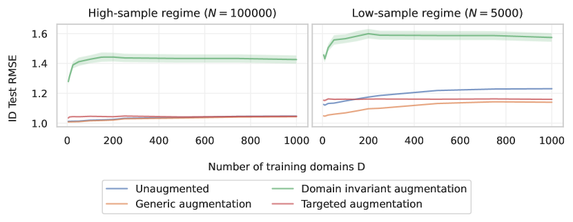
Figure 11: In-domain RMSE across values for $D$. Plots are averaged over 10 random seeds with standard errors.

Appendix E Experimental details

In this appendix, we provide tabular forms of results visualized in Figure 4. We also summarize core experimental details for each dataset, including hyperparameter tuning and model selection protocol.

E.1 Extended results

Table 5: Results on iWildCam2020-WILDS

	ID Test Macro F1	OOD Test Macro F1
Unaugmented	46.5 (0.4)	30.2 (0.3)
RandAugment	48.9 (0.2)	33.3 (0.2)
MixUp	45.5 (0.6)	28.9 (0.3)
CutMix	45.2 (0.7)	28.4 (0.5)
Cutout	47.9 (0.7)	32.6 (0.4)
LISA	45.4 (0.7)	29.6 (0.4)
CDAN	41.2 (0.6)	28.6 (0.2)
DeepCORAL	42.4 (1.2)	30.3 (0.6)
IRM	39.4 (0.4)	27.8 (0.1)
Copy-Paste (Same Y)	50.2 (0.7)	36.5 (0.4)

Table 6: Results on Camelyon17-WILDS

	ID Val Avg Acc	OOD Test Avg Acc
Unaugmented	89.3 (2.0)	65.2 (2.6)
RandAugment	94.9 (1.0)	75.3 (1.7)
MixUp	86.9 (2.2)	69.4 (2.1)
CutMix	84.7 (2.6)	60.9 (2.2)
LISA	91.0 (1.6)	73.6 (1.4)
DANN	86.1 (2.1)	64.5 (1.9)
DeepCORAL	92.3 (1.1)	62.3 (3.0)
IRM	88.0 (2.3)	62.4 (3.1)
Stain Color Jitter	96.7 (0.1)	90.5 (0.9)

Table 7: Results on BirdCalls

	ID Test Macro F1	OOD Test Macro F1
Unaugmented	70.0 (0.5)	27.8 (1.2)
SpecAugment	71.4 (0.4)	22.8 (1.0)
MixUp	74.0 (0.4)	26.3 (1.0)
LISA	69.7 (0.5)	29.4 (1.1)
Noise Reduction	75.4 (0.3)	31.6 (0.9)
Random Pass	71.2 (2.0)	31.8 (1.2)
CDAN	64.7 (0.5)	27.0 (1.2)
DeepCORAL	69.2 (0.5)	27.7 (0.9)
IRM	69.2 (0.4)	28.3 (0.8)
Color Jitter	73.8 (0.2)	26.1 (0.9)
Copy-Paste + Jitter (Region)	75.6 (0.3)	37.8 (1.0)

E.2 Hyperparameters

iWildCam.  All experiments used a ResNet-50, pretrained on ImageNet, with no weight decay and batch size 24, following Sagawa et al. (2021); Koh et al. (2021). Model selection and early stopping was done on the OOD validation split of iWildCam, which measures performance on a held-out set of cameras $\mathcal{D}^{\mathsf{val}}$, which is disjoint from both $\mathcal{D}^{\mathsf{train}}$ and $\mathcal{D}^{\mathsf{test}}$. We tuned all methods by fixing a budget of 10 tuning runs per method with one replicate each; the hyperparameter grids are given in Table 8. Final results are reported over 5 random seeds.

For CDAN, we tuned the classifier and discriminator learning rates and fixed the featurizer learning rate to be a tenth of the classifier’s, following Sagawa et al. (2021).

We applied all data augmentations stochastically with a tuned transform probability, since we found that doing so improved performance as in prior work (Gontijo-Lopes et al., 2020). For all augmentations, we also stochastically apply a random horizontal flip with the learned transform probability.

Table 8: Hyperparameter search spaces for methods on iWildCam2020-WILDS.

Method	Hyperparameters
ERM	Learning rate $\sim 10^{\text{Uni}(-5,-2)}$
Copy-Paste	Learning rate $\sim 10^{\text{Uni}(-5,-2)}$ Transform probability $\sim\text{Uni}(0.5,0.9)$
LISA	Learning rate $\sim 10^{\text{Uni}(-5,-2)}$ Transform probability $\sim\text{Uni}(0.5,0.9)$ Interpolation method $\in$ {MixUp, CutMix}
Vanilla MixUp	Learning rate $\sim 10^{\text{Uni}(-5,-2)}$ Transform probability $\sim\text{Uni}(0.5,0.9)$ $\alpha\in\{0.2,0.4\}$
Vanilla CutMix	Learning rate $\sim 10^{\text{Uni}(-5,-2)}$ Transform probability $\sim\text{Uni}(0.5,0.9)$ $\alpha\in\{0.5,1.0\}$
RandAugment	Learning rate $\sim 10^{\text{Uni}(-5,-2)}$ Transform probability $\sim\text{Uni}(0.5,0.9)$ $k\in\{1,2\}$
Cutout	Learning rate $\sim 10^{\text{Uni}(-5,-2)}$ Transform probability $\sim\text{Uni}(0.5,0.9)$ Version $\in$ {Original, Bounding box-aware}
CDAN	Classifier learning rate $\sim 10^{\text{Uni}(-5.5,-4)}$ Discriminator learning rate $\sim 10^{\text{Uni}(-5.5,-4)}$ $\lambda\sim 10^{\text{Uni}(-0.3,1)}$

Camelyon17.  All experiments used a randomly initialized DenseNet-121, with weight decay $0.01$ and batch size 168, following Sagawa et al. (2021); Koh et al. (2021). We also fixed the learning rate to that of Sagawa et al. (2021), which was selected by the authors of that paper after a random search over the distribution $10^{\text{Uni}(-4,-2)}$. For Camelyon17, we found that the choice of learning rate affected the relative ID vs. OOD accuracies of methods. To remove this confounder, we therefore standardized the learning rate across augmentations / algorithms for fair comparison. Separately tuning the learning rate for each algorithm did not significantly improve performance.

Because Camelyon17 is class-balanced, we ran experiments on DANN (rather than CDAN). For DANN, we used the learning rate fixed across all methods for the featurizer and set the classifier learning rate to be 10$\times$ higher, following Sagawa et al. (2021).

Because Camelyon17 has no ID test split, we report in-domain performance using the ID Val split.

Model selection and early stopping was done on the OOD validation split of Camelyon17, which measures performance on a held-out hospital $\mathcal{D}^{\mathsf{val}}$, which is disjoint from both $\mathcal{D}^{\mathsf{train}}$ and $\mathcal{D}^{\mathsf{test}}$. We tuned remaining hyperparameters by fixing a budget of 10 tuning runs per method with one replicate each; the hyperparameter grids are given in Table 9. Because of the large variance in performance between random seeds for some algorithms on Camelyon17 (Koh et al., 2021; Miller et al., 2021), we ran 20 replicates in the final results.

Table 9: Hyperparameter search spaces for methods on Camelyon17-WILDS.

Method	Hyperparameters
Stain Color Jitter	Augmentation strength $\in$ [0.05, 0.1]
LISA	Interpolation method $\in$ {MixUp, CutMix}
Vanilla MixUp	$\alpha\in\{0.2,0.4\}$
Vanilla CutMix	$\alpha\in\{0.5,1.0\}$
RandAugment	$k\in\{1,2\}$
Cutout	-
DANN	Discriminator learning rate $\sim 10^{\text{Uni}(-4,-2)}$ $\lambda\sim 10^{\text{Uni}(-1,0)}$

BirdCalls.  All experiments used an EfficientNet-B0, pretrained on ImageNet, with batch size 64. Model selection and early stopping was done on an ID validation split, which measures performance on a held-out examples from $\mathcal{D}^{\mathsf{train}}$. We tuned all methods by fixing a budget of 10 tuning runs per method with five replicates each; the hyperparameter grids are given in Table 10. Because of its small size, BirdCalls has relatively high variance between results; we thus report final results averaged over 20 random seeds.

For CDAN, we tuned the classifier and discriminator learning rates and fixed the featurizer learning rate to be a tenth of the classifier’s, matching our policy on iWildCam. For all augmentations, we also stochastically apply a random horizontal flip with the learned transform probability.

Table 10: Hyperparameter search spaces for methods on BirdCalls.

Method	Hyperparameters
ERM	Learning rate $\sim 10^{\text{Uni}(-4,-3)}$ Weight decay $\in\{0,0.001,0.1,1\}$
Copy-Paste	Learning rate $\sim 10^{\text{Uni}(-4,-3)}$ Weight decay $\in\{0,0.001,0.1,1\}$ Transform probability $\sim\text{Uni}(0.5,0.9)$
LISA	Learning rate $\sim 10^{\text{Uni}(-4,-3)}$ Weight decay $\in\{0,0.001,0.1,1\}$ Transform probability $\sim\text{Uni}(0.5,0.9)$
Vanilla MixUp	Learning rate $\sim 10^{\text{Uni}(-4,-3)}$ Weight decay $\in\{0,0.001,0.1,1\}$ Transform probability $\sim\text{Uni}(0.5,0.9)$ $\alpha\in\{0.2,0.4\}$
SpecAugment	Learning rate $\sim 10^{\text{Uni}(-4,-3)}$ Weight decay $\in\{0,0.001,0.1,1\}$ Transform probability $\sim\text{Uni}(0.5,0.9)$ $k\in\{1,2\}$ $F\in\{10,20,\cdots,100\}$ $T\in\{10,20,\cdots,100\}$
Random Pass	Learning rate $\sim 10^{\text{Uni}(-4,-3)}$ Weight decay $\in\{0,0.001,0.1,1\}$
Noise Reduction	Learning rate $\sim 10^{\text{Uni}(-4,-3)}$ Weight decay $\in\{0,0.001,0.1,1\}$
CDAN	Classifier learning rate $\sim 10^{\text{Uni}(-5,-2)}$ Weight decay $\in\{0,0.001,0.1,1\}$ Discriminator learning rate $\sim 10^{\text{Uni}(-5,-2)}$ $\lambda\sim 10^{\text{Uni}(-0.3,1)}$

E.3 CLIP Experiments

In our experiments finetuning CLIP on iWildCam and Camelyon17, we used OpenAI’s CLIP ViT-L/14 at 224 x 224 pixel resolution. Early stopping and model selection were done on the OOD validation splits. Hyperparameters are given in Table 11 for iWildCam and Table 12 for Camelyon17; we based Camelyon17 hyperparameters on Kumar et al. (2022) and iWildCam hyperparameters on Wortsman et al. (2022). We tuned all methods by fixing a budget of 10 tuning runs per method. Results are averaged over five seeds.

Table 11: Hyperparameter search spaces for CLIP experiments on iWildCam.

Method	Hyperparameters
ERM	Learning rate $\sim 10^{\text{Uni}(-6,-4)}$ Weight decay $\sim 10^{\text{Uni}(-4,-0.2)}$ Optimizer = AdamW
Copy-Paste (Same Y)	Learning rate $\sim 10^{\text{Uni}(-6,-4)}$ Weight decay $\sim 10^{\text{Uni}(-4,-0.2)}$ Transform probability $\sim\text{Uni}(0.5,0.9)$ Optimizer = AdamW

Table 12: Hyperparameter search spaces for CLIP experiments on Camelyon17.

Method	Hyperparameters
ERM	Learning rate $\sim 10^{\text{Uni}(-6,-3)}$ Weight decay $=0.01$ Optimizer = SGD
Stain Color Jitter	Learning rate $\sim 10^{\text{Uni}(-6,-3)}$ Weight decay $=0.01$ Augmentation strength $\in$ [0.05, 0.1] Optimizer = SGD

Appendix F Additional related work

Data augmentations for OOD robustness.  Prior work has sought to design augmentations specifically for robustness (Puli et al., 2022; Wang et al., 2022). Many augmentations are inspired by domain invariance and aim to randomize all domain-dependent features, including robust features $x_{\mathsf{d:robust}}$. For example, inter-domain MixUp interpolates inputs from different domains, possibly within the class (Wang et al., 2020; Xu et al., 2020; Yan et al., 2020; Yao et al., 2022). Ilse et al. (2021) propose to select transformations which maximally confuse a domain classifier. Several works train generative models to transform images between domains by learning to modify all domain-dependent features (Hoffman et al., 2018; Zhou et al., 2020b; Robey et al., 2021). In contrast, we preserve $x_{\mathsf{d:robust}}$ in targeted augmentations.

Targeted augmentations in the applied literature.  Many existing domain-specific augmentations can fit the proposed framework of targeted augmentations. For example, Stain Color Jitter is sourced from the biomedical literature and was designed for OOD robustness (Tellez et al., 2018, 2019; Miller et al., 2021). Copy-Paste (non-selective) has been previously applied to a smaller, single-habitat camera trap dataset (Beery et al., 2020). Our contribution lies in interpreting and formalizing why these targeted augmentations are effective OOD.

Underspecification.  D’Amour et al. (2020) point out the underspecification issue in out-of-domain generalization, in which multiple models are optimal on the training data, but generalize very differently out of domain. While our theoretical setting does not precisely fit the above definition of underspecification, we observe a related phenomenon; although there is a unique optimal model due to feature noise, OOD error can be high when the noiseless version of the regression problem is underspecified.

References

• Albuquerque et al. (2019) Albuquerque, I., Monteiro, J., Darvishi, M., Falk, T. H., and Mitliagkas, I. Generalizing to unseen domains via distribution matching. arXiv preprint arXiv:1911.00804, 2019.
• Arjovsky et al. (2019) Arjovsky, M., Bottou, L., Gulrajani, I., and Lopez-Paz, D. Invariant risk minimization. arXiv preprint arXiv:1907.02893, 2019.
• Bandi et al. (2018) Bandi, P., Geessink, O., Manson, Q., Van Dijk, M., Balkenhol, M., Hermsen, M., Bejnordi, B. E., Lee, B., Paeng, K., Zhong, A., et al. From detection of individual metastases to classification of lymph node status at the patient level: the camelyon17 challenge. IEEE transactions on medical imaging, 38(2):550–560, 2018.
• Beery et al. (2018) Beery, S., Van Horn, G., and Perona, P. Recognition in terra incognita. In Proceedings of the European conference on computer vision (ECCV), pp.  456–473, 2018.
• Beery et al. (2019) Beery, S., Morris, D., and Yang, S. Efficient pipeline for camera trap image review. arXiv preprint arXiv:1907.06772, 2019.
• Beery et al. (2020) Beery, S., Liu, Y., Morris, D., Piavis, J., Kapoor, A., Joshi, N., Meister, M., and Perona, P. Synthetic examples improve generalization for rare classes. In Proceedings of the IEEE/CVF Winter Conference on Applications of Computer Vision, pp.  863–873, 2020.
• Beery et al. (2021) Beery, S., Agarwal, A., Cole, E., and Birodkar, V. The iwildcam 2021 competition dataset. arXiv preprint arXiv:2105.03494, 2021.
• Birodkar et al. (2021) Birodkar, V., Lu, Z., Li, S., Rathod, V., and Huang, J. The surprising impact of mask-head architecture on novel class segmentation. In Proceedings of the IEEE/CVF International Conference on Computer Vision, pp.  7015–7025, 2021.
• Chen et al. (2021a) Chen, Q., Shui, C., and Marchand, M. Generalization bounds for meta-learning: An information-theoretic analysis. Advances in Neural Information Processing Systems, 34:25878–25890, 2021a.
• Chen et al. (2020) Chen, S., Dobriban, E., and Lee, J. H. A group-theoretic framework for data augmentation. The Journal of Machine Learning Research, 21(1):9885–9955, 2020.
• Chen et al. (2021b) Chen, Y., Rosenfeld, E., Sellke, M., Ma, T., and Risteski, A. Iterative feature matching: Toward provable domain generalization with logarithmic environments. arXiv preprint arXiv:2106.09913, 2021b.
• Cubuk et al. (2020) Cubuk, E. D., Zoph, B., Shlens, J., and Le, Q. V. Randaugment: Practical automated data augmentation with a reduced search space. In Proceedings of the IEEE/CVF conference on computer vision and pattern recognition workshops, pp.  702–703, 2020.
• D’Amour et al. (2020) D’Amour, A., Heller, K., Moldovan, D., Adlam, B., Alipanahi, B., Beutel, A., Chen, C., Deaton, J., Eisenstein, J., Hoffman, M. D., et al. Underspecification presents challenges for credibility in modern machine learning. Journal of Machine Learning Research, 2020.
• Dao et al. (2019) Dao, T., Gu, A., Ratner, A., Smith, V., De Sa, C., and Ré, C. A kernel theory of modern data augmentation. In International Conference on Machine Learning, pp. 1528–1537. PMLR, 2019.
• Denton et al. (2022) Denton, T., Wisdom, S., and Hershey, J. R. Improving bird classification with unsupervised sound separation. In ICASSP 2022-2022 IEEE International Conference on Acoustics, Speech and Signal Processing (ICASSP), pp.  636–640. IEEE, 2022.
• DeVries & Taylor (2017) DeVries, T. and Taylor, G. W. Improved regularization of convolutional neural networks with cutout. arXiv preprint arXiv:1708.04552, 2017.
• Ganin et al. (2016) Ganin, Y., Ustinova, E., Ajakan, H., Germain, P., Larochelle, H., Laviolette, F., Marchand, M., and Lempitsky, V. Domain-adversarial training of neural networks. The journal of machine learning research, 17(1):2096–2030, 2016.
• Gontijo-Lopes et al. (2020) Gontijo-Lopes, R., Smullin, S. J., Cubuk, E. D., and Dyer, E. Affinity and diversity: Quantifying mechanisms of data augmentation. arXiv preprint arXiv:2002.08973, 2020.
• Gulrajani & Lopez-Paz (2020) Gulrajani, I. and Lopez-Paz, D. In search of lost domain generalization. arXiv preprint arXiv:2007.01434, 2020.
• Györfi et al. (2002) Györfi, L., Kohler, M., Krzyzak, A., Walk, H., et al. A distribution-free theory of nonparametric regression, volume 1. Springer, 2002.
• He et al. (2019) He, Z., Xie, L., Chen, X., Zhang, Y., Wang, Y., and Tian, Q. Data augmentation revisited: Rethinking the distribution gap between clean and augmented data. arXiv preprint arXiv:1909.09148, 2019.
• Hendrycks et al. (2021) Hendrycks, D., Basart, S., Mu, N., Kadavath, S., Wang, F., Dorundo, E., Desai, R., Zhu, T., Parajuli, S., Guo, M., et al. The many faces of robustness: A critical analysis of out-of-distribution generalization. In Proceedings of the IEEE/CVF International Conference on Computer Vision, pp.  8340–8349, 2021.
• Hoffman et al. (2018) Hoffman, J., Tzeng, E., Park, T., Zhu, J.-Y., Isola, P., Saenko, K., Efros, A., and Darrell, T. Cycada: Cycle-consistent adversarial domain adaptation. In International conference on machine learning, pp. 1989–1998. Pmlr, 2018.
• Hopping et al. (2022) Hopping, W. A., Kahl, S., and Klinck, H. A collection of fully-annotated soundscape recordings from the Southwestern Amazon Basin, September 2022. URL https://doi.org/10.5281/zenodo.7079124.
• Hsu et al. (2011) Hsu, D., Kakade, S. M., and Zhang, T. An analysis of random design linear regression. arXiv preprint arXiv:1106.2363, 2011.
• Ilse et al. (2021) Ilse, M., Tomczak, J. M., and Forré, P. Selecting data augmentation for simulating interventions. In International Conference on Machine Learning, pp. 4555–4562. PMLR, 2021.
• Joly et al. (2021) Joly, A., Goëau, H., Kahl, S., Picek, L., Lorieul, T., Cole, E., Deneu, B., Servajean, M., Durso, A., Bolon, I., et al. Overview of lifeclef 2021: an evaluation of machine-learning based species identification and species distribution prediction. In Experimental IR Meets Multilinguality, Multimodality, and Interaction: 12th International Conference of the CLEF Association, CLEF 2021, Virtual Event, September 21–24, 2021, Proceedings, pp.  371–393. Springer, 2021.
• Jose & Simeone (2021) Jose, S. T. and Simeone, O. Information-theoretic generalization bounds for meta-learning and applications. Entropy, 23(1):126, 2021.
• Kahl et al. (2022) Kahl, S., Charif, R., and Klinck, H. A collection of fully-annotated soundscape recordings from the Northeastern United States, August 2022. URL https://doi.org/10.5281/zenodo.7079380.
• Koh et al. (2021) Koh, P. W., Sagawa, S., Marklund, H., Xie, S. M., Zhang, M., Balsubramani, A., Hu, W., Yasunaga, M., Phillips, R. L., Gao, I., et al. Wilds: A benchmark of in-the-wild distribution shifts. In International Conference on Machine Learning, pp. 5637–5664. PMLR, 2021.
• Kumar et al. (2022) Kumar, A., Shen, R., Bubeck, S., and Gunasekar, S. How to fine-tune vision models with sgd. arXiv preprint arXiv:2211.09359, 2022.
• Long et al. (2018) Long, M., Cao, Z., Wang, J., and Jordan, M. I. Conditional adversarial domain adaptation. Advances in neural information processing systems, 31, 2018.
• Lyle et al. (2020) Lyle, C., van der Wilk, M., Kwiatkowska, M., Gal, Y., and Bloem-Reddy, B. On the benefits of invariance in neural networks. arXiv preprint arXiv:2005.00178, 2020.
• Mahajan et al. (2021) Mahajan, D., Tople, S., and Sharma, A. Domain generalization using causal matching. In International Conference on Machine Learning, pp. 7313–7324. PMLR, 2021.
• Miller et al. (2021) Miller, J. P., Taori, R., Raghunathan, A., Sagawa, S., Koh, P. W., Shankar, V., Liang, P., Carmon, Y., and Schmidt, L. Accuracy on the line: on the strong correlation between out-of-distribution and in-distribution generalization. In International Conference on Machine Learning, pp. 7721–7735. PMLR, 2021.
• Navine et al. (2022) Navine, A., Kahl, S., Tanimoto-Johnson, A., Klinck, H., and Hart, P. A collection of fully-annotated soundscape recordings from the Island of Hawai’i, September 2022. URL https://doi.org/10.5281/zenodo.7078499.
• Park et al. (2019) Park, D. S., Chan, W., Zhang, Y., Chiu, C.-C., Zoph, B., Cubuk, E. D., and Le, Q. V. Specaugment: A simple data augmentation method for automatic speech recognition. arXiv preprint arXiv:1904.08779, 2019.
• Puli et al. (2022) Puli, A., Joshi, N., He, H., and Ranganath, R. Nuisances via negativa: Adjusting for spurious correlations via data augmentation. arXiv preprint arXiv:2210.01302, 2022.
• Radford et al. (2021) Radford, A., Kim, J. W., Hallacy, C., Ramesh, A., Goh, G., Agarwal, S., Sastry, G., Askell, A., Mishkin, P., Clark, J., et al. Learning transferable visual models from natural language supervision. In International conference on machine learning, pp. 8748–8763. PMLR, 2021.
• Robey et al. (2021) Robey, A., Pappas, G. J., and Hassani, H. Model-based domain generalization. Advances in Neural Information Processing Systems, 34:20210–20229, 2021.
• Rosenfeld et al. (2020) Rosenfeld, E., Ravikumar, P., and Risteski, A. The risks of invariant risk minimization. arXiv preprint arXiv:2010.05761, 2020.
• Ruifrok et al. (2001) Ruifrok, A. C., Johnston, D. A., et al. Quantification of histochemical staining by color deconvolution. Analytical and quantitative cytology and histology, 23(4):291–299, 2001.
• Sagawa et al. (2021) Sagawa, S., Koh, P. W., Lee, T., Gao, I., Xie, S. M., Shen, K., Kumar, A., Hu, W., Yasunaga, M., Marklund, H., et al. Extending the wilds benchmark for unsupervised adaptation. arXiv preprint arXiv:2112.05090, 2021.
• Sainburg (2022) Sainburg, T. Noise reduction in python using spectral gating, 2022. URL https://github.com/timsainb/noisereduce.
• Sun & Saenko (2016) Sun, B. and Saenko, K. Deep coral: Correlation alignment for deep domain adaptation. In European conference on computer vision, pp.  443–450. Springer, 2016.
• Sun et al. (2017) Sun, B., Feng, J., and Saenko, K. Correlation alignment for unsupervised domain adaptation. In Domain Adaptation in Computer Vision Applications, pp. 153–171. Springer, 2017.
• Tellez et al. (2018) Tellez, D., Balkenhol, M., Otte-Höller, I., van de Loo, R., Vogels, R., Bult, P., Wauters, C., Vreuls, W., Mol, S., Karssemeijer, N., et al. Whole-slide mitosis detection in h&e breast histology using phh3 as a reference to train distilled stain-invariant convolutional networks. IEEE transactions on medical imaging, 37(9):2126–2136, 2018.
• Tellez et al. (2019) Tellez, D., Litjens, G., Bándi, P., Bulten, W., Bokhorst, J.-M., Ciompi, F., and van der Laak, J. Quantifying the effects of data augmentation and stain color normalization in convolutional neural networks for computational pathology. Medical image analysis, 58, 2019.
• Wang et al. (2022) Wang, R., Yi, M., Chen, Z., and Zhu, S. Out-of-distribution generalization with causal invariant transformations. In Proceedings of the IEEE/CVF Conference on Computer Vision and Pattern Recognition, pp.  375–385, 2022.
• Wang et al. (2020) Wang, Y., Li, H., and Kot, A. C. Heterogeneous domain generalization via domain mixup. In ICASSP 2020-2020 IEEE International Conference on Acoustics, Speech and Signal Processing (ICASSP), pp.  3622–3626. IEEE, 2020.
• Wiles et al. (2021) Wiles, O., Gowal, S., Stimberg, F., Rebuffi, S.-A., Ktena, I., Dvijotham, K. D., and Cemgil, A. T. A fine-grained analysis on distribution shift. In International Conference on Learning Representations, 2021.
• Wortsman et al. (2022) Wortsman, M., Ilharco, G., Gadre, S. Y., Roelofs, R., Gontijo-Lopes, R., Morcos, A. S., Namkoong, H., Farhadi, A., Carmon, Y., Kornblith, S., et al. Model soups: averaging weights of multiple fine-tuned models improves accuracy without increasing inference time. In International Conference on Machine Learning, pp. 23965–23998. PMLR, 2022.
• Xu et al. (2020) Xu, M., Zhang, J., Ni, B., Li, T., Wang, C., Tian, Q., and Zhang, W. Adversarial domain adaptation with domain mixup. In Proceedings of the AAAI Conference on Artificial Intelligence, volume 34, pp.  6502–6509, 2020.
• Yan et al. (2020) Yan, S., Song, H., Li, N., Zou, L., and Ren, L. Improve unsupervised domain adaptation with mixup training. arXiv preprint arXiv:2001.00677, 2020.
• Yao et al. (2022) Yao, H., Wang, Y., Li, S., Zhang, L., Liang, W., Zou, J., and Finn, C. Improving out-of-distribution robustness via selective augmentation. arXiv preprint arXiv:2201.00299, 2022.
• Yun et al. (2019) Yun, S., Han, D., Oh, S. J., Chun, S., Choe, J., and Yoo, Y. Cutmix: Regularization strategy to train strong classifiers with localizable features. In Proceedings of the IEEE/CVF international conference on computer vision, pp.  6023–6032, 2019.
• Zhang et al. (2017) Zhang, H., Cisse, M., Dauphin, Y. N., and Lopez-Paz, D. mixup: Beyond empirical risk minimization. arXiv preprint arXiv:1710.09412, 2017.
• Zhou et al. (2020a) Zhou, K., Yang, Y., Hospedales, T., and Xiang, T. Deep domain-adversarial image generation for domain generalisation. In Proceedings of the AAAI Conference on Artificial Intelligence, volume 34, pp.  13025–13032, 2020a.
• Zhou et al. (2020b) Zhou, K., Yang, Y., Hospedales, T., and Xiang, T. Learning to generate novel domains for domain generalization. In European conference on computer vision, pp.  561–578. Springer, 2020b.
• Zhu (2012) Zhu, S. A short note on the tail bound of wishart distribution. arXiv preprint arXiv:1212.5860, 2012.