Reinforcement Learning for Combining Search Methods
in the Calibration of Economic ABMs

Abstract.

Calibrating agent-based models (ABMs) in economics and finance typically involves a derivative-free search in a very large parameter space. In this work, we benchmark a number of search methods in the calibration of a well-known macroeconomic ABM on real data, and further assess the performance of ”mixed strategies” made by combining different methods. We find that methods based on random-forest surrogates are particularly efficient, and that combining search methods generally increases performance since the biases of any single method are mitigated. Moving from these observations, we propose a reinforcement learning (RL) scheme to automatically select and combine search methods on-the-fly during a calibration run. The RL agent keeps exploiting a specific method only as long as this keeps performing well, but explores new strategies when the specific method reaches a performance plateau. The resulting RL search scheme outperforms any other method or method combination tested, and does not rely on any prior information or trial and error procedure.

1. Introduction and literature review

The last decades have witnessed a consistent growth of the reach and scope of agent-based models (ABMs) in economics and finance, certainly also as a consequence of continuing improvements in the computer hardware and software that form the foundation over which ABMs are designed and used (Axtell and Farmer, 2022). ABMs have also become mature enough that they have seen adoption and usage within central banks and other financial institutions for specific tasks (Turrell, 2016; Plassard et al., 2020). A particularly noteworthy application domain is the modelling of the housing market, pioneered by Bank of England (Baptista et al., 2016) and later studied by many other central banks (Cokayne, 2019; Catapano et al., 2021; Carro, 2022; Méro et al., 2022), and the macroeconomic model proposed in (Poledna et al., 2023) and recently adopted by Bank of Canada (Hommes et al., 2022). Other successful applications can be found in the modelling of financial stability (Bookstaber et al., 2014; Covi et al., 2020), or of the banking sector (Chan-Lau, 2017). Finally, ABMs for economic and financial markets are currently being investigated, extended, and possibly used, within JPMorgan Chase (Ardon et al., 2021; Vadori et al., 2022; Ardon et al., 2023).

In spite of these success stories, ABMs still occupy a minor for modelling in economics and finance. One fundamental reason behind ABMs’ limited adoption is the overwhelming flexibility of such a modelling tool which, if handled incorrectly, can lead to widely different models of the same phenomenon and consequently to a narrow predictive power.

Rigorous calibration of ABMs via large amounts of real data is a promising path to address the problem of ABM flexibility by appropriately restricting it in data-driven and systematic manner (Axtell and Farmer, 2022). In fact, ABM calibration has a long history (Fagiolo et al., 2007), but interest in ABM calibration has grown particularly in recent times of ever-increasing data abundance. Historically, the problem has been approached mostly via the ‘method of simulated moments’ (Gilli and Winker, 2003; Franke, 2009; Grazzini and Richiardi, 2015), which involves minimising a measure of distance between summary statistics of real and simulated time series, while more recently, other approaches based on maximum likelihood or Bayesian statistics have been proposed and successfully tested (Grazzini et al., 2017; Platt, 2021; Dyer et al., 2022; Monti et al., 2023).

A common challenge of all calibration frameworks is the need of efficiently searching for optimal parameter combinations in high-dimensional spaces, a problem made particularly arduous by the high computational cost of state-of-the-art ABM simulations. This is why the use of several heuristic search methods has been proposed in the ABM literature. Specifically, in (Lamperti et al., 2018), building on the work of (Conti and O’Hagan, 2010), the authors propose the use of machine surrogates, specifically in the form of XG-boost regressors, to suggest promising parameter combinations by interpolating the results of previously computed ABM simulations. In (Angione et al., 2022), the authors expand on this idea and test the ability of several machine learning surrogate algorithms such as Gaussian processes, random forests and support vector machines, to reproduce ABM simulation data. In (Platt, 2020) the author instead proposes the use of particle swarm samplers (Kaveh, 2017; Stonedahl, 2011), as well as the search heuristic of (Knysh and Korkolis, 2016).

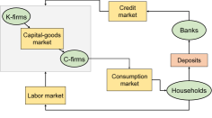
(a)

(b)

Figure 1. The CATS model. (a) An illustration of the agent classes of the model and their interactions. Agent classes are represented in green ovals, interaction types are specified in rectangles, and markets are specified in yellow rectangles. The directions of the arrows indicate the flow of the specific good e.g., consumption-goods are acquired by households from C-firms, while labour is acquired by firms from households. (b) An illustration of the firms’ decisions on the price-quantity space. Prices $P_{i,t}$ and quantities $Y_{i,t}$ of goods are updated following the 4 solid black arrows, and not the dashed black arrows. The dashed blue line is the minimum price they can charge, corresponding to the average cost ($AC$) for production.

In this work, we take a different view of the problem and test the performance of existing search strategies, on a common calibration task, and propose simple methods to combine them in mixed strategies to drastically boost calibration performance. We test our methods one of the most well-known and studied macroeconomic ABMs (Delli Gatti et al., 2011; Assenza et al., 2015; Dawid and Delli Gatti, 2018), often referred to as the CATS (“Complex Adaptive Trivial System”) model. Our contributions are as follows:

• We verify that the macroeconomic ABM considered can be efficiently calibrated to reproduce a variety of real time series.

• We find that methods based on random forest machine learning surrogates are particularly effective searchers in the highly non-convex and discretely-changing loss function induced by ABMs.

• We find that combining together different search methods almost always provides better overall performance, and propose this as a convenient heuristic to apply in the ABM calibration practice.

• We introduce a simple reinforcement-learning technique to automatically aggregate any number of search methods in a single mixed strategy, and demonstrate the superior performance of this approach with respect to naive aggregation strategies.

In Section 2 we overview the main features of the CATS model, in Section 3 we describe the calibration technique considered and the search methods that we employ individually and in combination, in Section 4 we describe our benchmarking experiments and the results obtained, in Section 5 we describe the reinforcement learning scheme we proposed to automatically combine existing methods, and demonstrate its performance, in Section 6 we verify that the calibrated model reproduces the target real data and that our findings hold well against changes in the model and in the loss function, in Section 7 we conclude.

2. Model illustration

The CATS model consists of four classes of interacting agents: households, final-goods producing firms (C-firms), capital producing firms (K-firms) and banks. Figure 1a illustrates these classes of agents and the markets through which they interact, while Figure 1b illustrates a distinctive feature of the model, i.e., the decision making operated by firms on price and quantity of goods to produce. In the interest of space, and since this work focuses on the calibration of the model, we do not describe the details of the model here and refer the reader to (Assenza et al., 2015) for an in-depth exposition.

3. Calibration description

The calibration method we consider is composed of three main steps. First, a search method (from now on also called a sampler) suggests a set of parameters to explore, then a number of simulations are performed for each selected parameter, and finally a loss function is evaluated to measure the goodness of fit of the simulations with respect to the real time series. Iterating these three steps allows finding parameters corresponding to progressively lower loss values, and the parameter corresponding to the lowest loss value can be considered optimal.

We follow the method of moments paradigm (Franke, 2009; Chen and Lux, 2018) and use the following loss function (often called distance in the ABM literature) for all calibrations. This takes the form

(1) $$L=\frac{1}{D}\sum_{d=1}^{D}\mathbf{g}_{d}^{\rm{T}}\mathbf{W}_{d}\mathbf{g}_{d},$$

where $\mathbf{g}_{d}$ is the vector of difference between the real and the simulated moments of the one-dimensional time series $d$, and $D$ is the total number of dimensions in the multi-dimensional time series considered. Different choices for the weighting matrices $\mathbf{W}_{d}$ have been proposed in the literature (Franke, 2009; Franke and Westerhoff, 2012). In this work we take the $\mathbf{W}_{d}$ matrices to be diagonal matrices with elements $(\mathbf{W}_{d})_{ii}$ inversely proportional to the square of the real $i$-th moment of the one-dimensional time series $d$. This choice guarantees that the same weight is given to all moments considered, independently of the different scales or units of measure that the different moments might have. In essence, the loss function written in this way provides an estimate of the relative squared error between real and simulated moments.

Since we use a common loss function for all calibrations, the only difference between the calibration runs considered here is the choice of search method. We consider the following five search methods, all of which are implemented in Black-it (Benedetti et al., 2022), an open source library for ABM calibration:  

Halton sampler $\mathsf{(}\mathsf{H}\mathsf{)}$. This sampler suggests points according to the Halton series (Halton, 1964; Kocis and Whiten, 1997). The Halton series is a low-discrepancy series providing a quasi-random sampling that guarantees an evenly distributed coverage of the parameter space. As the method is very similar to a purely random search, we use it as a baseline for the more advanced search strategies analysed.

Random forest sampler $\mathsf{(}\mathsf{RF}\mathsf{)}$. This sampler is a type of machine learning surrogate sampler. It interpolates the previously computed loss values using a random forest classifier (Bajer et al., 2015), and it then proposes parameters in the vicinity of the lowest values of the interpolated loss surface.

XG-boost sampler $\mathsf{(}\mathsf{XB}\mathsf{)}$. This sampler is a machine learning surrogate sampler that interpolates loss values using an XG-Boost regression (Chen and Guestrin, 2016), as proposed in (Lamperti et al., 2018).

Gaussian process sampler $\mathsf{(}\mathsf{GP}\mathsf{)}$. This sampler is a machine learning surrogate sampler that interpolates loss values using a Gaussian process regression (Conti and O’Hagan, 2010; Rasmussen, 2004).

Best batch sampler $\mathsf{(}\mathsf{BB}\mathsf{)}$. This sampler is a very essential type of genetic algorithm (Stonedahl, 2011) that takes the parameters corresponding to the current lowest loss values and perturbs them slightly in a purely random fashion to suggest new parameter values to explore.

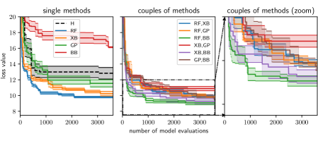
Method	H	RF	XB	GP	BB	RF,XB	RF,GP	RF,BB	XB,GP	XB,BB	GP,BB
Mean	12.83	9.803	10.24	11.96	16.87	9.88	9.861	9.07	10.89	9.27	9.83
Std. Err.	0.73	0.094	0.29	0.51	0.59	0.16	0.075	0.24	0.27	0.31	0.26

Figure 2. Top graphs: Loss as a function of the number of model evaluations for the single methods (left), and for couples of methods (middle and right). Bottom table: Means and standard errors of the lowest losses achieved by the different strategies. Note that these results are directly comparable with those shown in Figure 3 and discussed in the next section, as both $x$ and $y$ axes have identical ranges.

4. Benchmarking experiments

Param.	Description	Range
$\xi$	Memory parameter in consumption	0.5-1
$\chi$	Wealth parameter in consumption	0-0.5
$\rho$	Quantity adjustment	0-1
$\bar{\eta}$	Price adjustment	0-1
$\mu$	Bank’s gross mark-up	1-1.5
$\zeta$	Bank’s leverage	0-0.01
$\delta^{k}$	Inventories depreciation rate	0-0.5
$\gamma$	Fraction of investing C-firms	0-0.5
$\theta$	Rate of debt reimbursement	0-0.1
$\nu$	Memory parameter in investment	0-1
$t_{w}$	Tax rate	0-0.4

Table 1. Parameter descriptions and their ranges.

Experiments preparation. Similarly to (Delli Gatti and Grazzini, 2020), we calibrate the model using the following 5 historical time series, representing the US economy from 1948 to 2019, downloaded from the FRED database (McCracken and Ng, 2016): total output, personal consumption, gross private investment (all in real terms), the implicit price deflator and the civilian unemployment. To make simulated and observed data comparable, we remove the trend component from the total output, consumption and investment using an HP filter (Ravn and Uhlig, 2002); and we use simulated and observed price deflator to compute de-meaned inflation rates. In Table 1 we list the 11 parameters considered for calibration and the specified ranges of variation.

Experiments performed. Using the four samplers described in the previous section, we build 11 search methods as the 5 samplers taken individually, as well as the 6 combinations of any two non-baseline samplers. For each search method, we perform 3 independent calibration runs. Each calibration run consists of 3600 model evaluations, and for each parameter 5 independent simulations are performed to reduce the statistical variance of the loss estimate. Each simulated series consists of 800 time-steps generated by running the model for 1100 time steps and discarding the first 300. This makes up a total of almost 600000 simulations and more than 50 days of CPU time, which we were able to compress in less than two days by leveraging parallel computing both within and between calibrations.

Results and discussion. Figure 2 reports the cumulative minimum loss achieved by the different sampling strategies as a function of the number of model evaluations performed. The lines and the shaded areas indicate averages and standard errors over the 3 realisations of the experiment. Single samplers are reported in the left graph, while couples of samplers are reported in the middle graph as well as –zoomed– in the right graph. The table at the bottom of the graphs reports the minimum loss achieved by the different methods.

Single methods. When samplers are taken in isolation, the random forest sampler ($\mathsf{RF}$) clearly outperforms all other methods, the XG-boost sampler ($\mathsf{XB}$) is the second best performing and the Gaussian process sampler ($\mathsf{GP}$) is substantially worse than the other two machine learning surrogate samplers. The low performance of the $\mathsf{GP}$ sampler can be ascribed to the smoothness and regularity assumptions inherent in Gaussian process regression models, assumptions that are not present in random-forest or XG-boost models, and not suited to describe the roughed and complex loss landscape of ABM calibrations. The best batch sampler ($\mathsf{BB}$) performs very poorly in isolation, and underperforms even in comparison with the baseline $\mathsf{H}$ sampler. This is not entirely surprising, since the $\mathsf{BB}$ sampler can only propose small perturbations around current loss minima and can thus easily remain stuck in one of the many local minima of the highly non-convex landscape typical of ABMs loss functions.

Couples of methods. All methods, not just the poorly performing $\mathsf{BB}$ sampler, possess intrinsic sampling biases that in the long run can hinder their performances and make them converge to sub-optimal solutions. We find that combining different methods in mixed strategies can strongly mitigate such biases and improve overall performance. The effect can be observed in the second and third panel of Figure 2, by noticing that couples of methods, with the only exception of the ‘$\mathsf{XB},\mathsf{GP}$’ combination, always perform on par or better than the best single samplers ($\mathsf{RF}$ and $\mathsf{XB}$). Interestingly, the best overall performances are achieved by coupling one machine learning surrogate sampler with the genetic $\mathsf{BB}$ sampler. In light of the above discussion, we note that machine learning surrogate samplers and the $\mathsf{BB}$ sampler work in very different ways, and hence their combination can strongly diminish the respective sampling biases, while since machine learning surrogates all work in similar ways, their combination does not yield to comparable improvements. The $\mathsf{RF},\mathsf{BB}$ and the $\mathsf{XB},\mathsf{BB}$ combinations are particularly effective and achieve the lowest loss values.

To summarise, our results show that the $\mathsf{RF}$ and $\mathsf{XB}$ samplers are particularly well suited to efficiently search in the parameter space of ABMs. The success of the $\mathsf{RF}$ and $\mathsf{XB}$ samplers can be ascribed to the ability to correctly approximate high dimensional and possibly discontinuous functions with no regularities. However, the performance of the $\mathsf{RF}$ and $\mathsf{XB}$ samplers can be significantly improved if they are used in combination with the $\mathsf{BB}$ sampler.

In the next section, we move a step forward and consider the combination of multiple methods in more general terms, without limiting ourselves to the simplest scenario of a “round-robin” selection.

5. Reinforcement learning experiments

The results of the benchmarks presented in Section 4 show that the combination of different types of sampling methods can be beneficial for the calibration process even when we naively alternate the available sampling methods during the course of a calibration. This suggests that the investigation of different –and more flexible– scheduling policies of search methods could bring to even more efficient calibrations.

In particular, it is desirable that the chosen scheduling policy shows some form of adaptivity, i.e. that is able to choose the sampling method with more chances to sample a good parameter vector, taking into account the progress of the calibration process. To achieve this goal, we frame the ABM calibration problem as a reinforcement learning (RL) problem where the decision-maker (the agent) has to find a good policy such that it chooses the most promising search method, where “promising” is related to the chances of sampling a parameter that improves the value of the loss. The decision-maker receives feedback for its choice in the form of a reward signal computed from the sampled loss function values. This is what makes the scheduling policy adaptive: search methods that more often provide loss improvements are more rewarding from the decision-maker perspective, and they have more chances of being chosen in the next calibration step; on the other hand, whenever a search method does not show to be rewarding anymore, then the decision-maker can detect this and switch the preference to another search method.

Specifically, we frame the calibration process as a multi-armed bandit (MAB) problem (Katehakis and Veinott Jr, 1987; Weber, 1992; Auer et al., 2002a; Berry and Fristedt, 1985; Gittins et al., 2011; Lattimore and Szepesvári, 2020). This is a classic reinforcement learning problem that exemplifies the exploration–exploitation trade-off dilemma (Sutton and Barto, 2018). The challenge for the agent is to simultaneously attempt to acquire new knowledge by “exploring” different actions and optimise their decisions based on existing knowledge by “exploiting” actions that have been estimated to be rewarding. We define the different sampling methods as the actions available for the agent, and loss improvements as the reward signals. More formally, we define the reward at time $t$ as the fractional improvement achieved over the previous best loss

(2) $$R_{t}=\max\{0,\frac{L_{\mathsf{best},t-1}-L_{t}}{L_{\mathsf{best},t-1}}\}$$

where $L_{t}$ is the loss obtained for the simulations sampled at time $t$, and $L_{\mathsf{best},t-1}$ is the best loss sampled up to time $t-1$. Note that $R_{t}$ is a random variable, because $L_{t}$ depends on the simulated time series outputted by the ABM, and the chosen parameter vector. As in most of the MAB problems, the goal for the agent is to maximize the cumulative sum of rewards

(3) $$S_{N}=\sum\limits_{t=1}^{N}R_{t},$$

where $N$ is the number of calibration steps.

Differently from the usual MAB setting, the reward probability distributions associated to each available sampler are obviously non-stationary (Auer et al., 2002b), and in fact they change drastically during the course of the calibration. As an example, consider that at end of a calibration all methods –even the best ones– stop providing any improvement in the loss, and hence the reward distributions become progressively more peaked around zero.

The MAB is a very simple framework for RL problems, that are more generally modelled as Markov Decision Processes (MDPs) (Sutton and Barto, 2018). However, their simplicity is precisely what makes MAB better suited for our context than other approaches. Indeed, as MAB algorithms focus on finding the best action at each step rather than learning the entire environment, they are much more sample efficient. In the ABM calibration context, simulations are typically very expensive, and consequently the sample efficiency of the learning method is of paramount importance.

In the following, we test our MAB framework in two experiments. First, in the offline-learning experiments, we let the agent learn from the previously executed calibrations of Section 4. Then, in the online-learning experiments, we let the agent interact with the environment and optimise its policy on-the-fly during each calibration.

Sampler \ Context	sing. samp.	glob.	high $L_{\mathsf{best},t}$	low $L_{\mathsf{best},t}$
$\mathsf{RF}$	0.25	0.27	1.3	0.052
$\mathsf{XB}$	0.23	0.23	0.61	0.033
$\mathsf{GP}$	0.21	0.17	0.26	0.068
$\mathsf{BB}$	0.11	0.23	0.28	0.18
$\mathsf{H}$	0.20	0.20	0.24	N.A.

Table 2. The estimated $Q$ functions for the different search methods and under different contexts. (sing. samp.) uses only single sample calibrations, (glob.) uses all calibrations, (high $L_{\mathsf{best},t}$) uses all calibration but only actions taken when the loss is above the median loss, and (low $L_{\mathsf{best},t}$) uses all calibration but only actions taken when the loss is below the median loss. Results are reported on a scale of $10^{-3}$.

Offline experiments. In this section, we train a MAB agent over past calibration histories. More precisely, we take the single methods and couples of methods calibrations of Section 4, and process them as if they were observed by a MAB algorithm. This approach gives us an estimate of the expected gain of each sampler, and therefore information about the effectiveness of the sampler methods on the specific calibration task.

In the context of MAB solutions, action-value methods are methods for estimating the values of actions and for using the estimates to make action selection decisions (Sutton and Barto, 2018). Let $Q(a)$ be the value of action $a$ or, in our context, the value of using a specific search method during a calibration. One natural way to estimate such values is by averaging the rewards actually received

(4) $$Q(a)=\frac{\sum\limits_{t=1}^{N}R_{t}\cdot\mathds{1}_{A_{t}=a}}{\sum\limits_{t=1}^{N}\mathds{1}_{A_{t}=a}},$$

where $A_{t}$ is the action chosen at step $t$. This approach is often called the sample-average method (Sutton and Barto, 2018).

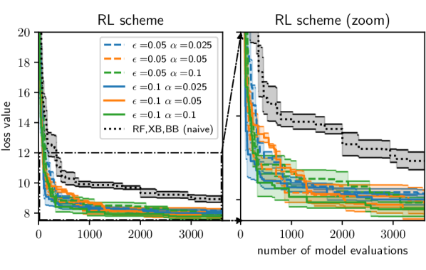
$\epsilon\backslash\,\alpha$	0.025	0.05	0.1
0.05	$8.148\pm 0.089$	$7.94\pm 0.28$	$7.93\pm 0.12$
0.1	$8.00\pm 0.13$	$\textbf{7.77}\pm 0.23$	$\textbf{7.77}\pm 0.17$

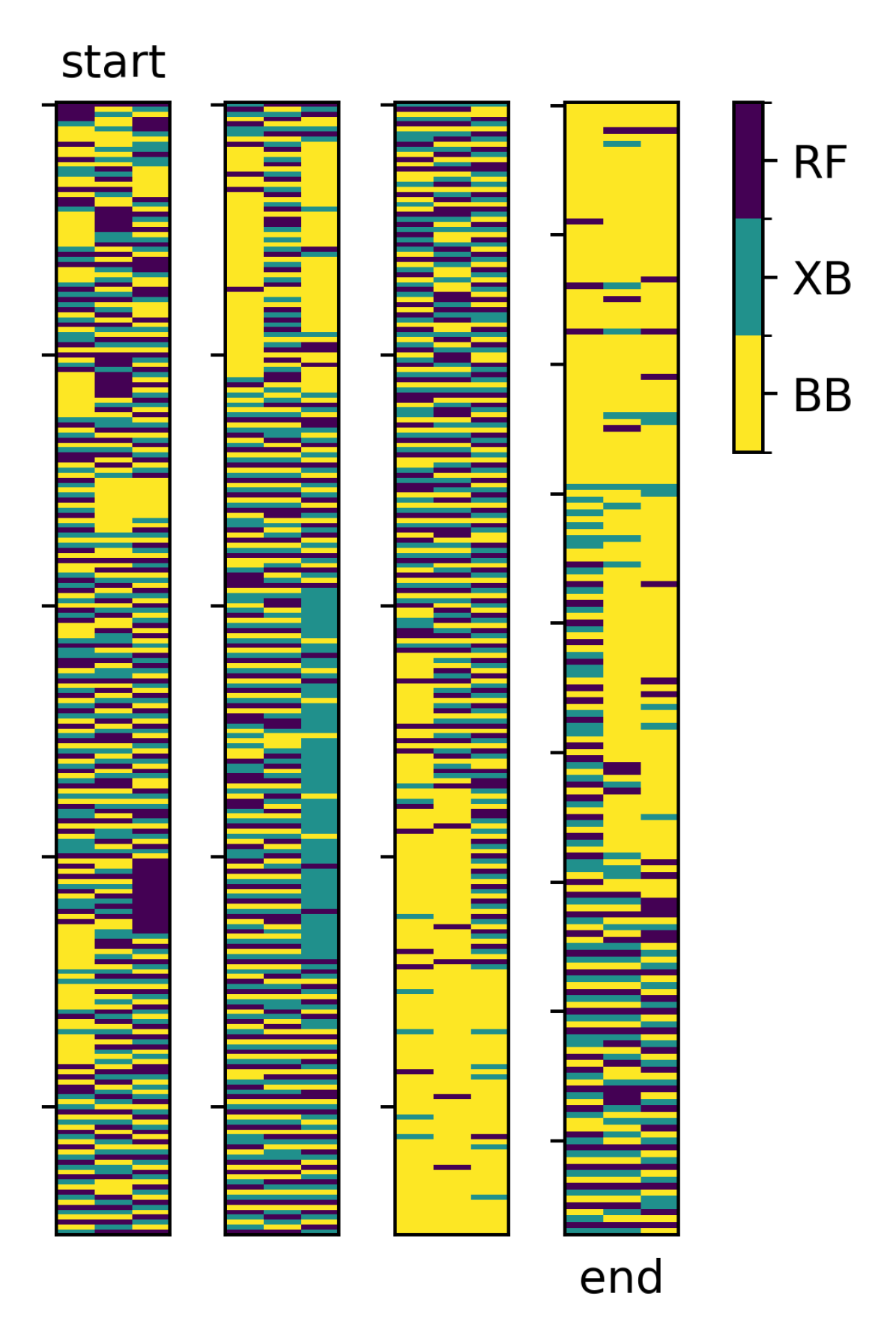
Figure 3. Top graphs: (left and middle) Loss as a function of the number of model evaluations for the RL scheme with different choices of parameters and for a naive alternation of the samplers, (right) the specific samplers (‘actions’) selected by the RL scheme with parameters $\epsilon=0.1$ and $\alpha=0.1$ during the 900 epochs of a calibration for each of the 3 independent runs, to be read from left to right, from top to bottom, note that each epoch provides 4 model evaluations. Bottom table: Means and standard errors of the lowest losses achieved by the RL scheme. These results can be compared directly with those of Figure 2 as they have identical ranges on both $x$ and the $y$ axes.

The first two columns of Table 2 provide the results of this analysis when only the single sampler calibrations are considered (“sing. samp.” column) and when all calibrations are considered (“glob.” column). Not surprisingly, the $\mathsf{RF}$ sampler reaches the highest $Q$ value using both datasets, and the results of the “sing. samp.” column replicate the hierarchy of samplers of the first panel of Figure 2. Interestingly, the value of the $\mathsf{BB}$ sampler dramatically increases when the combined dataset is used, confirming the analysis carried forward in the last section on the effectiveness of using the $\mathsf{BB}$ sampler in combination with a machine learning surrogate sampler.

The third and fourth columns of Table 2 offer additional insight. In these columns, we restrict the value function estimation of Eq. (4) to actions performed in one of two different ‘states’, characterised by the best loss $L_{\mathsf{best},t}$ being either above the median (“high $L_{\mathsf{best},t}$” column) or below the median (“low $L_{\mathsf{best},t}$” column). Models of this kind, where the actions of a MAB agent depend on one or more states (in this case high/low loss value) are known as contextual MABs (Langford and Zhang, 2007; Li et al., 2010).

The results clearly indicate that when the loss is high (typically at the beginning of the calibration) the optimal action is the $\mathsf{RF}$ sampler, but when the loss is low (typically at the end of the calibration) the optimal action becomes, by far, the $\mathsf{BB}$ sampler. The $\mathsf{BB}$ sampler proposes small perturbations around low-loss parameter combinations, and hence it can be expected to be particularly effective when the calibration has already reached a good minimum, which can be further explored with this method.

This analysis suggests the design of a mixed search scheme that exploits a machine learning surrogate sampler (say $\mathsf{RF}$ or $\mathsf{XB}$) when the loss is sufficiently high, before switching to the $\mathsf{BB}$ sampler towards the end of the calibration. However, this specific strategy would not be generally applicable as, on a new calibration task, one would not know in advance the loss values that can be achieved, and hence could not set any loss threshold on the choice of sampler. In the following section, we show how a MAB agent trained on-the-fly can solve this problem by learning this behaviour, without any prior information, during the course of a single calibration run.

Online experiments. In online learning schemes, the agent interacts with the environment through a specific policy $\pi$ while simultaneously optimising the policy. We propose the use of one of the most well-known algorithms for online learning of MAB agents in non-stationary environments: the $\epsilon$-greedy policy with fixed learning rate (Sutton and Barto, 2018). In this framework, at each step $t$, with large probability $1-\epsilon$ the agent performs a ‘greedy’ action i.e., it selects the action $a$ with the highest value $Q(a)$, and with small probability $\epsilon$ it selects a purely random action. We can hence write down the $\epsilon$-greedy MAB policy as follows

(5) $$\pi_{t}=\begin{cases}\operatorname*{argmax}_{a}\,Q_{t}(a)&\text{with probability }1-\epsilon\\ \text{random action}&\text{with probability }\epsilon\end{cases}.$$

After the selected action $a$ is performed, the agent receives a reward $R_{t}$, and updates the value $Q_{t}(a)$ as

(6) $$Q_{t+1}(a)=\alpha R_{t}+(1-\alpha)Q_{t}(a),$$

where $\alpha$ is referred to as the learning rate. Note that the above update rule can be seen as an exponentially weighted moving average of the rewards obtained through action $a$. The exponential weighting guarantees that the current value of the $Q$ function is not substantially affected by rewards received many steps earlier and, in turn, this allows the algorithm to adapt to changes of the environment on-the-fly during a calibration.

Figure 3 shows the results obtained when using the described scheme with a set of possible actions given by the tree samplers $\mathsf{RF}$, $\mathsf{XB}$ and $\mathsf{BB}$. The left and middle panels of the figure can be directly compared with the graphs in Figure 2, as they have identical ranges on both $x$ and $y$ axes. We see that the RL scheme proposed strongly outperforms any other method, or method combination, tested in the previous section. This happens for all values considered for the parameters $\epsilon$ and $\alpha$, with the best results –by a very narrow margin– obtained with $\epsilon=\alpha=0.1$. For comparison, the figure also reports –in a black dotted curve– the loss achieved by combining the three samplers $\mathsf{RF}$, $\mathsf{XB}$ and $\mathsf{BB}$ in a simple (‘naive’) alternation. Such a simple method alternation, with no use of RL, can be imagined to provide a lower-bound on the performance of the RL scheme, and it is seen to give rise to a significantly slower convergence.

The right panel of Figure 3 helps us build intuition around the performance of the RL scheme proposed. It depicts with different colours the different actions (samplers) selected during the 3 RL calibration runs performed with parameters $\epsilon=\alpha=0.1$. At the beginning of the calibration (say, the first two columns), the agent explores the different strategies by alternating between the 3 samplers and sometimes exploits a specific sampler with long streaks of identical sampler choices. Towards the end of the calibration (say, the last two columns), when the loss is low, the agent instead more decisively exploits the $\mathsf{BB}$ sampler, in agreement with the offline experiments described earlier and summarised in Table 2.

In conclusion, we find that modelling the calibration process as an online learning MAB problem, with actions being given by different available search methods, allows to detect the most promising search methods during the course of a single calibration. This gives rise to a very efficient scheme, and represents a practical tool to intelligently combine different search methods.

We also explored more sophisticated MAB learning schemes including ‘kl-UCB’ (Garivier and Cappé, 2011), ‘Exp3’ (Bubeck et al., 2012), and ‘Discounted Thompson’ sampling (Raj and Kalyani, 2017), but found no substantial improvements. Hence, we believe that the $\epsilon$-greedy –fixed learning rate– algorithm described should be preferred both because of its simplicity and because of its great computational efficiency which, in turn, implies the absence of any overhead in using the RL scheme over naive method combinations.

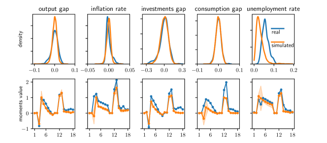
Figure 4. A comparison between distributions and moments of the real series (blue) and the simulated series of lowest loss (orange). The first row reports density estimates obtained via a kernel density estimator. The second row reports the value of the moments. In the second row, the indices from 1 to 18 on the $x$-axis represent the following statistics. 1-4): mean, variance, skewness and kurtosis, 5-9): autocorrelations of increasing time lags. 10-14): mean, variance, skewness and kurtosis of the differentiated time series, 14-18): autocorrelations of the differentiated time series.

6. Validation

Calibrated model. We here verify that the calibrated model is able to approximately reproduce the behaviour of the five variables tracked in the real dataset. This can be immediately seen by analysing Figure 4, in which the distribution and the moments of the simulated series with the lowest loss are compared with those computed for the real historical series. In agreement with (Delli Gatti and Grazzini, 2020), output, consumption and investment are very well captured by the CATS model, while stronger deviations can be observed in inflation and unemployment rates. Also in agreement with (Delli Gatti and Grazzini, 2020) we find that, in general, the CATS model can only partially account for the persistence of the real time series. This is clear from the fact that the simulated series have systematically lower values of virtually all autocorrelations considered (indices 5-9 and 14-18 in the second-row graphs). It is important to note here that the calibration experiments performed in this work do not incur into problems of overfitting since the number of parameters and the flexibility of the ABM considered are limited in comparison to the details of the real time series analysed. This fact is evident from the discrepancy between the high order moments of the real and simulated series in Figure 4, as well as from the fact that the loss never reaches zero in Figures 2 and 3.

Different models. While the focus of the current work is on the calibration of the CATS model, we verified that our findings hold also for other ABMs. Specifically, in Figure 5 we show the results of similar calibration experiments for two other toy models: the paradigmatic ‘Brock and Hommes’ asset pricing model (Brock and Hommes, 1998) with a method of moments loss, and a SIR model on a small-world network topology (Simoes et al., 2008) with a Euclidean distance loss. In agreement with the rest of this work, we find that the $\mathsf{RF}$ sampler is the best-performing sampler when methods are used in isolation, that coupling different samplers generally provides better performances, and that our RL-scheme can be successfully used to intelligently combine search methods. However, these alternative calibration tasks are much simpler than the calibration of the CATS model considered in the rest of this work. For this reason, we do not see a significant performance improvement in using RL combinations over simple combinations but, importantly, we consistently find the performance of the RL-scheme to be as good as the best samplers or sampler-combinations tested, without requiring any trial and error.

Reproducibility. In the interest of reproducibility an easy-to-use implementation of the reinforcement learning scheduler proposed in this work has been released in open source within the Black-it package.

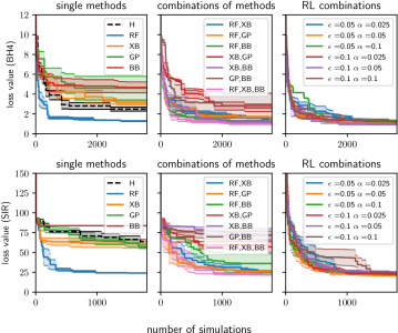
Figure 5. Loss as a function of the number of model evaluations for single methods, simple method combinations, and RL method combinations, for the BH4 model (Brock and Hommes, 1998) with a method of moments loss (1st row) and for the SIR model with a Euclidean distance loss (2nd row).

7. Conclusions

In this work, we systematically compare the performance of 5 search strategies, taken in isolation and in combination, on a method-of-moments calibration of a standard macroeconomic ABM. Our results show that calibration based on machine learning surrogate samplers, of the kind proposed in (Lamperti et al., 2018) but using a random forest algorithm for interpolation, provides superior performance with respect to the other search methods. Our results further show that coupling different search methods together gives rise to search strategies that typically improve over their constituents. The empirical efficacy of random forest search methods and of combining different search methods can be of practical help to researchers interested in calibrating and using medium and large-scale ABMs. However, when combining different search methods a natural issue arises about which methods should be combined, and in which way.

We provide a solution to this issue by framing the choice of search methods as a multi-armed bandit problem, and leveraging a well-known reinforcement learning scheme to select the best method on-the-fly during the course of a single calibration. The RL scheme proposed outperforms any other method or method combination tested, and thus provides a practical tool for researchers interested in efficiently calibrating ABMs.

In the future, it would be interesting to deepen the analyses of the present study in two possible lines of research, based on either extensions of the banchmarking experiments of Section 4 or on further investigations into the RL scheme of Section 5.

The benchmarking framework could be extended in several dimensions. The first is the testing of other standard search methods, such as particle swarm samplers or machine learning samplers based on neural networks. The second is the inclusion in the analysis of other measures of goodness of fit, in addition to the method of moments, such as likelihood measures, Bayesian measures (Grazzini et al., 2017; Dyer et al., 2022), or information theoretic measures (Lamperti, 2018). The third is the addition of other widely known macroeconomic ABMs (Dawid and Delli Gatti, 2018) to the analysis, such as the so-called “K+S” model (Dosi et al., 2010), or the recent large-scale model of (Poledna et al., 2023). This would allow quantitative benchmarking not only of the calibration strategies, but also of the different models when calibrated on the same data. The final direction would involve appropriately increasing the data on which the ABMs are calibrated and tested, potentially with more variables and with more national economies. In essence, while the present work is an important step towards a systematic assessment calibration methods for medium and large-scale economic ABMs, all of the above mentioned directions would surely represent equally important steps towards an increasingly more data-driven ABM development.

The RL scheme proposed may also deserve further specific investigation. For example, one could verify whether the RL search method developed here maintains its high performance also in the more general setting of black-box function optimisation, perhaps in other specific application domains that might have peculiarities similar to the ABM calibration problem. One might also try to extend the simple (yet effective) MAB framework introduced here, by providing more ‘contextual’ information to the agent and hence attempting to represent the ABM calibration problem either as an online contextual-MAB problem, or directly as a partially-observable MDP (Kaelbling et al., 1998).

- (1)
- Angione et al. (2022) Claudio Angione, Eric Silverman, and Elisabeth Yaneske. 2022. Using machine learning as a surrogate model for agent-based simulations. Plos one 17, 2 (2022), e0263150.
- Ardon et al. (2021) Leo Ardon, Nelson Vadori, Thomas Spooner, Mengda Xu, Jared Vann, and Sumitra Ganesh. 2021. Towards a fully RL-based Market Simulator. In Proceedings of the Second ACM International Conference on AI in Finance. 1–9.
- Ardon et al. (2023) Leo Ardon, Jared Vann, Deepeka Garg, Thomas Spooner, and Sumitra Ganesh. 2023. Phantom-A RL-driven Multi-Agent Framework to Model Complex Systems. In Proceedings of the 2023 International Conference on Autonomous Agents and Multiagent Systems. 2742–2744.
- Assenza et al. (2015) Tiziana Assenza, Domenico Delli Gatti, and Jakob Grazzini. 2015. Emergent dynamics of a macroeconomic agent based model with capital and credit. Journal of Economic Dynamics and Control 50 (2015), 5–28. https://doi.org/10.1016/j.jedc.2014.07.001 Crises and Complexity.
- Auer et al. (2002a) Peter Auer, Nicolo Cesa-Bianchi, and Paul Fischer. 2002a. Finite-time analysis of the multiarmed bandit problem. Machine learning 47, 2 (2002), 235–256.
- Auer et al. (2002b) Peter Auer, Nicolò Cesa-Bianchi, Yoav Freund, and Robert E. Schapire. 2002b. The Nonstochastic Multiarmed Bandit Problem. SIAM J. Comput. 32, 1 (2002), 48–77.
- Axtell and Farmer (2022) Robert L Axtell and J Doyne Farmer. 2022. Agent-based modeling in economics and finance: Past, present, and future. Journal of Economic Literature (2022).
- Bajer et al. (2015) Lukáš Bajer, Zbyněk Pitra, and Martin Holeňa. 2015. Benchmarking Gaussian processes and random forests surrogate models on the BBOB noiseless testbed. In Proceedings of the Companion Publication of the 2015 Annual Conference on Genetic and Evolutionary Computation. 1143–1150.
- Baptista et al. (2016) Rafa Baptista, J Doyne Farmer, Marc Hinterschweiger, Katie Low, Daniel Tang, and Arzu Uluc. 2016. Macroprudential policy in an agent-based model of the UK housing market. (2016).
- Benedetti et al. (2022) Marco Benedetti, Gennaro Catapano, Francesco De Sclavis, Marco Favorito, Aldo Glielmo, Davide Magnanimi, and Antonio Muci. 2022. Black-it: A Ready-to-Use and Easy-to-Extend Calibration Kit for Agent-based Models. Journal of Open Source Software 7, 79 (2022), 4622. https://doi.org/10.21105/joss.04622
- Berry and Fristedt (1985) Donald A Berry and Bert Fristedt. 1985. Bandit problems: sequential allocation of experiments (Monographs on statistics and applied probability). London: Chapman and Hall 5, 71-87 (1985), 7–7.
- Bookstaber et al. (2014) Richard Bookstaber, Mark Paddrik, and Brian Tivnan. 2014. An agent-based model for financial vulnerability. Technical Report. Office of Financial Research Working Paper Series.
- Brock and Hommes (1998) William A Brock and Cars H Hommes. 1998. Heterogeneous beliefs and routes to chaos in a simple asset pricing model. Journal of Economic dynamics and Control 22, 8-9 (1998), 1235–1274.
- Bubeck et al. (2012) Sébastien Bubeck, Nicolo Cesa-Bianchi, et al. 2012. Regret analysis of stochastic and nonstochastic multi-armed bandit problems. Foundations and Trends® in Machine Learning 5, 1 (2012), 1–122.
- Carro (2022) Adrian Carro. 2022. Could Spain be less different? Exploring the effects of macroprudential policy on the house price cycle. (2022).
- Catapano et al. (2021) Gennaro Catapano, Francesco Franceschi, Michele Loberto, and Valentina Michelangeli. 2021. Macroprudential policy analysis via an agent based model of the real estate sector. Bank of Italy Temi di Discussione (Working Paper) No 1338 (2021).
- Chan-Lau (2017) Mr Jorge A Chan-Lau. 2017. ABBA: An agent-based model of the banking system. International Monetary Fund.
- Chen and Guestrin (2016) Tianqi Chen and Carlos Guestrin. 2016. Xgboost: A scalable tree boosting system. In Proceedings of the 22nd acm sigkdd international conference on knowledge discovery and data mining. 785–794.
- Chen and Lux (2018) Zhenxi Chen and Thomas Lux. 2018. Estimation of sentiment effects in financial markets: A simulated method of moments approach. Computational Economics 52, 3 (2018), 711–744.
- Cokayne (2019) Graeme Cokayne. 2019. The effects of macroprudential policies on house price cycles in an agent-based model of the Danish housing market. Technical Report. Danmarks Nationalbank Working Papers.
- Conti and O’Hagan (2010) Stefano Conti and Anthony O’Hagan. 2010. Bayesian emulation of complex multi-output and dynamic computer models. Journal of statistical planning and inference 140, 3 (2010), 640–651.
- Covi et al. (2020) G Covi, M Montagna, and G Torri. 2020. On the Origins of Systemic Risk. Technical Report. European Central Bank Working Papers.
- Dawid and Delli Gatti (2018) Herbert Dawid and Domenico Delli Gatti. 2018. Agent-based macroeconomics. Handbook of computational economics 4 (2018), 63–156.
- Delli Gatti et al. (2011) Domenico Delli Gatti, Saul Desiderio, Edoardo Gaffeo, Pasquale Cirillo, and Mauro Gallegati. 2011. Macroeconomics from the Bottom-up. Vol. 1. Springer Science & Business Media.
- Delli Gatti and Grazzini (2020) Domenico Delli Gatti and Jakob Grazzini. 2020. Rising to the challenge: Bayesian estimation and forecasting techniques for macroeconomic Agent Based Models. Journal of Economic Behavior & Organization 178 (2020), 875–902.
- Dosi et al. (2010) Giovanni Dosi, Giorgio Fagiolo, and Andrea Roventini. 2010. Schumpeter meeting Keynes: A policy-friendly model of endogenous growth and business cycles. Journal of Economic Dynamics and Control 34, 9 (2010), 1748–1767.
- Dyer et al. (2022) Joel Dyer, Patrick Cannon, J Doyne Farmer, and Sebastian Schmon. 2022. Black-box Bayesian inference for economic agent-based models. arXiv preprint arXiv:2202.00625 (2022).
- Fagiolo et al. (2007) Giorgio Fagiolo, Alessio Moneta, and Paul Windrum. 2007. A critical guide to empirical validation of agent-based models in economics: Methodologies, procedures, and open problems. Computational Economics 30, 3 (2007), 195–226.
- Franke (2009) Reiner Franke. 2009. Applying the method of simulated moments to estimate a small agent-based asset pricing model. Journal of Empirical Finance 16, 5 (2009), 804–815.
- Franke and Westerhoff (2012) Reiner Franke and Frank Westerhoff. 2012. Structural stochastic volatility in asset pricing dynamics: Estimation and model contest. Journal of Economic Dynamics and Control 36, 8 (2012), 1193–1211.
- Garivier and Cappé (2011) Aurélien Garivier and Olivier Cappé. 2011. The KL-UCB algorithm for bounded stochastic bandits and beyond. In Proceedings of the 24th annual conference on learning theory. JMLR Workshop and Conference Proceedings, 359–376.
- Gilli and Winker (2003) Manfred Gilli and Peter Winker. 2003. A global optimization heuristic for estimating agent based models. Computational Statistics & Data Analysis 42, 3 (2003), 299–312.
- Gittins et al. (2011) John Gittins, Kevin Glazebrook, and Richard Weber. 2011. Multi-armed bandit allocation indices. John Wiley & Sons.
- Grazzini and Richiardi (2015) Jakob Grazzini and Matteo Richiardi. 2015. Estimation of ergodic agent-based models by simulated minimum distance. Journal of Economic Dynamics and Control 51 (2015), 148–165.
- Grazzini et al. (2017) Jakob Grazzini, Matteo G Richiardi, and Mike Tsionas. 2017. Bayesian estimation of agent-based models. Journal of Economic Dynamics and Control 77 (2017), 26–47.
- Halton (1964) John H Halton. 1964. Algorithm 247: Radical-inverse quasi-random point sequence. Commun. ACM 7, 12 (1964), 701–702.
- Hommes et al. (2022) Cars Hommes, Mario He, Sebastian Poledna, Melissa Siqueira, and Yang Zhang. 2022. CANVAS: A Canadian Behavioral Agent-Based Model. Technical Report. Bank of Canada.
- Kaelbling et al. (1998) Leslie Pack Kaelbling, Michael L Littman, and Anthony R Cassandra. 1998. Planning and acting in partially observable stochastic domains. Artificial intelligence 101, 1-2 (1998), 99–134.
- Katehakis and Veinott Jr (1987) Michael N Katehakis and Arthur F Veinott Jr. 1987. The multi-armed bandit problem: decomposition and computation. Mathematics of Operations Research 12, 2 (1987), 262–268.
- Kaveh (2017) Ali Kaveh. 2017. Particle swarm optimization. In Advances in Metaheuristic Algorithms for Optimal Design of Structures. Springer, 11–43.
- Knysh and Korkolis (2016) Paul Knysh and Yannis Korkolis. 2016. Blackbox: A procedure for parallel optimization of expensive black-box functions. arXiv preprint arXiv:1605.00998 (2016).
- Kocis and Whiten (1997) Ladislav Kocis and William J Whiten. 1997. Computational investigations of low-discrepancy sequences. ACM Transactions on Mathematical Software (TOMS) 23, 2 (1997), 266–294.
- Lamperti (2018) Francesco Lamperti. 2018. An information theoretic criterion for empirical validation of simulation models. Econometrics and Statistics 5 (2018), 83–106.
- Lamperti et al. (2018) Francesco Lamperti, Andrea Roventini, and Amir Sani. 2018. Agent-based model calibration using machine learning surrogates. Journal of Economic Dynamics and Control 90 (2018), 366–389.
- Langford and Zhang (2007) John Langford and Tong Zhang. 2007. The epoch-greedy algorithm for contextual multi-armed bandits. Advances in neural information processing systems 20, 1 (2007), 96–1.
- Lattimore and Szepesvári (2020) Tor Lattimore and Csaba Szepesvári. 2020. Bandit algorithms. Cambridge University Press.
- Li et al. (2010) Lihong Li, Wei Chu, John Langford, and Robert E. Schapire. 2010. A Contextual-Bandit Approach to Personalized News Article Recommendation. In Proceedings of the 19th international conference on World wide web - WWW ’10. 661. https://doi.org/10.1145/1772690.1772758 arXiv:1003.0146 [cs].
- McCracken and Ng (2016) Michael W McCracken and Serena Ng. 2016. FRED-MD: A monthly database for macroeconomic research. Journal of Business & Economic Statistics 34, 4 (2016), 574–589.
- Méro et al. (2022) Bence Méro, András Borsos, Zsuzsanna Hosszú, Zsolt Oláh, and Nikolett Vágó. 2022. A high resolution agent-based model of the hungarian housing market. MNB Working Papers 7 (2022).
- Monti et al. (2023) Corrado Monti, Marco Pangallo, Gianmarco De Francisci Morales, and Francesco Bonchi. 2023. On learning agent-based models from data. Scientific Reports 13, 1 (2023), 9268.
- Plassard et al. (2020) Romain Plassard et al. 2020. Making a Breach: The Incorporation of Agent-Based Models into the Bank of England’s Toolkit. Technical Report. Groupe de REcherche en Droit, Economie, Gestion (GREDEG CNRS), Université ….
- Platt (2020) Donovan Platt. 2020. A comparison of economic agent-based model calibration methods. Journal of Economic Dynamics and Control 113 (2020), 103859.
- Platt (2021) Donovan Platt. 2021. Bayesian estimation of economic simulation models using neural networks. Computational Economics (2021), 1–52.
- Poledna et al. (2023) Sebastian Poledna, Michael Gregor Miess, Cars Hommes, and Katrin Rabitsch. 2023. Economic forecasting with an agent-based model. European Economic Review 151 (2023), 104306.
- Raj and Kalyani (2017) Vishnu Raj and Sheetal Kalyani. 2017. Taming non-stationary bandits: A Bayesian approach. arXiv preprint arXiv:1707.09727 (2017).
- Rasmussen (2004) Carl Edward Rasmussen. 2004. Gaussian processes in machine learning. Springer.
- Ravn and Uhlig (2002) Morten O Ravn and Harald Uhlig. 2002. On adjusting the Hodrick-Prescott filter for the frequency of observations. Review of economics and statistics 84, 2 (2002), 371–376.
- Simoes et al. (2008) Marcos Simoes, MM Telo da Gama, and André Nunes. 2008. Stochastic fluctuations in epidemics on networks. Journal of the Royal Society Interface 5, 22 (2008), 555–566.
- Stonedahl (2011) Forrest J Stonedahl. 2011. Genetic algorithms for the exploration of parameter spaces in agent-based models. Ph. D. Dissertation. Northwestern University.
- Sutton and Barto (2018) Richard S Sutton and Andrew G Barto. 2018. Reinforcement learning: An introduction. MIT press.
- Turrell (2016) Arthur Turrell. 2016. Agent-based models: understanding the economy from the bottom up. Bank of England Quarterly Bulletin (2016), Q4.
- Vadori et al. (2022) Nelson Vadori, Leo Ardon, Sumitra Ganesh, Thomas Spooner, Selim Amrouni, Jared Vann, Mengda Xu, Zeyu Zheng, Tucker Balch, and Manuela Veloso. 2022. Towards Multi-Agent Reinforcement Learning driven Over-The-Counter Market Simulations. arXiv preprint arXiv:2210.07184 (2022).
- Weber (1992) Richard Weber. 1992. On the Gittins index for multiarmed bandits. The Annals of Applied Probability (1992), 1024–1033.