SCF-FDPS: A Fast $N$-body Code for Simulating Disk-halo Systems

Abstract

A fast $N$-body code has been developed for simulating a stellar disk embedded in a live dark matter halo. In generating its Poisson solver, a self-consistent field (SCF) code which inherently possesses perfect scalability is incorporated into a tree code which is parallelized using a library termed Framework for Developing Particle Simulators (FDPS). Thus, the code developed here is called SCF-FDPS. This code has realized the speedup of a conventional tree code by applying an SCF method not only to the calculation of the self-gravity of the halo but also to that of the gravitational interactions between the disk and halo particles. Consequently, in the SCF-FDPS code, a tree algorithm is applied only to calculate the self-gravity of the disk. On a many-core parallel computer, the SCF-FDPS code has performed at least three times, in some case nearly an order of magnitude, faster than an extremely-tuned tree code on it, if the numbers of disk and halo particles are, respectively, fixed for both codes. In addition, the SCF-FDPS code shows that the cpu cost scales almost linearly with the total number of particles and almost inversely with the number of cores. We find that the time evolution of a disk-halo system simulated with the SCF-FDPS code is, in large measure, similar to that obtained using the tree code. We suggest how the present code can be extended to cope with a wide variety of disk-galaxy simulations.

1 Introduction

The number of particles in $N$-body simulations of astronomical objects like galaxies has been increasing, in step with the progress in parallel computing technology. This remarkable development has brought a great benefit to disk-galaxy simulations, because galactic disks are rotation-supported, cold systems, so that a sufficiently large number of particles are needed for the disk to sidestep the heating originating from Poisson noise. In fact, Fujii et al. (2011) have demonstrated that a spiral feature emerging in a disk surrounded by an unresponsive halo is fading away gradually over time for a million-particle simulation, while it persists until late times for a three-million-particle simulation. On the other hand, Athanassoula (2002) has revealed that for a given disk-halo model, the disk is stabilized against bar formation when the halo is rigid, while a large-amplitude bar is excited through a wave-particle resonance between a bar mode in the disk and halo particles when the halo is live. This fact coerces us to deal with a halo as self-gravitating. In making a halo live for a disk-halo system, the mass of a halo particle has to be made equal to that of a disk particle to avoid the shot noise generated by halo particles when they pass through the disk. Unfortunately, a halo mass is estimated to be at least around an order of magnitude larger than a disk mass, because a halo is considered to extend far beyond the optical edge of the disk on the basis of the observed rotation curves of disk galaxies that are, in general, flat out to large radii (e.g., Sofue & Rubin, 2001). Consequently, the number of halo particles becomes larger than that of disk particles by an order of magnitude or many more. It thus follows that disk-galaxy simulations inevitably demand a large number of particles.

As the number of particles in $N$-body simulation increases, the number of force calculation increases accordingly. Because a given particle receives the gravitational force from all other particles in an $N$-particle system, the number of the total force calculation reaches $\mathcal{O}(N^{2})$ at every time step in the simplest way. This explosive nature in force calculation is alleviated down to $\mathcal{O}(N\log N)$ by the introduction of a tree algorithm developed by Barnes & Hut (1986). Indeed, recent large $N$-body simulations of disk galaxies are based on a tree code. For example, Dubinski et al. (2009) adopted a parallelized tree code to investigate the bar instability in galactic disks using $1.8\times 10^{7}$ particles for a disk and $10^{8}$ particles for a halo, while D’Onghia et al. (2013) used a tree-based gravity solver to examine the origin of spiral structure in disk galaxies with $10^{8}$ particles for a disk immersed in a rigid halo. Furthermore, Fujii et al. (2018) have employed a tree-based code called BONSAI (Bédorf et al., 2012) optimized for Graphics Processing Units to scrutinize the dynamics of disk galaxies which consist of live disk, bulge, and halo components with the total number of particles being increased up to $5\times 10^{8}$. In their subsequent work, Fujii et al. (2019) have boosted the total number of particles up to $8\times 10^{9}$ to construct the Milky Way Galaxy model that reproduces the observed properties.

As mentioned above, a tree algorithm is commonly used to study disk galaxies with a huge number of particles. In such a situation, a faster tree code is understandably desirable from various aspects of numerical studies. As computer architecture is shifted to parallelized one, a tree code has been adjusted to a parallel computer. Above all, a numerical library termed Framework for Developing Particle Simulators (FDPS) (Iwasawa et al., 2016; Namekata et al., 2018) has tuned a tree code to the utmost limit of a massively memory-distributed parallel computer. Therefore, no further speedup of existing tree codes is expected on their own.

We then try to incorporate a self-consistent field (SCF) code into a tree code. Of course, the FDPS library is implemented in the tree part of the resulting hybrid code for the efficient parallelization. In an SCF approach, Poisson’s equation is solved by expanding the density and potential of the system being studied in a set of basis functions. In particular, owing to the expansion of the full spatial dependence, the cpu cost becomes $\mathcal{O}(N)$. Moreover, because the perfect scalability is inherent in the SCF approach, it is suitable for parallel computing. By taking advantage of these characteristics, we will be able to accelerate $N$-body simulations of disk galaxies using a hybrid code named SCF-FDPS in which an SCF code is incorporated into an FDPS-implemented tree code (Hozumi et al., 2023).

In this paper, we describe how an SCF code is incorporated into a tree code, and show how well the resulting SCF-FDPS code works. In Section 2, we present the details of the SCF-FDPS code, including how an SCF approach is applied to a disk-halo system. In Section 3, along with the determination of the parameters inherent in the code, the performance of the code is shown. In Section 4, we discuss the extension of the present code to cope with a wide variety of disk-galaxy simulations. Conclusions are given in Section 5.

2 Details of the SCF-FDPS Code

We develop a fast $N$-body code which is based on both SCF and tree approaches. First, we explain the SCF method briefly, and then, describe the details of the SCF-FDPS code.

2.1 SCF Method

An SCF method requires a biorthonormal basis set which satisfies Poisson’s equation written by

$$\nabla^{2}\Phi_{nlm}(\bm{r})=4\pi G\rho_{nlm}(\bm{r}),$$ (1)

where $\rho_{nlm}(\bm{r})$ and $\Phi_{nlm}(\bm{r})$ are, respectively, the density and potential basis functions at the position vector of a particle, $\bm{r}$, with $n$ being the ‘quantum’ number in the radial direction and with $l$ and $m$ being corresponding quantities in the angular directions. Here, the biorthonormality is represented by

$$\int\rho_{nlm}(\bm{r})\,[\Phi_{n^{\prime}l^{\prime}m^{\prime}}(\bm{r})]^{*}d\bm{r}=\delta_{nn^{\prime}}\delta_{ll^{\prime}}\delta_{mm^{\prime}},$$ (2)

where $\delta_{kk^{\prime}}$ is the Kronecker delta defined by $\delta_{kk^{\prime}}=0$ for $k\neq k^{\prime}$ and $\delta_{kk^{\prime}}=1$ for $k=k^{\prime}$.

With the help of such a biorthonormal basis set as is noted above, the density and potential of the system are expanded, respectively, by the corresponding basis functions as

$$\rho(\bm{r})=\sum_{n,l,m}\,A_{nlm}\,\rho_{nlm}(\bm{r})$$ (3)

and

$$\Phi(\bm{r})=\sum_{n,l,m}A_{nlm}\,\Phi_{nlm}(\bm{r}),$$ (4)

where $A_{nlm}$ are the expansion coefficients at time $t$. When the potential basis functions are operated on the density field that is expanded as Equation (3), $A_{nlm}$ are given, via the biorthonormality relation of Equation (2), by

$$A_{nlm}=\int\rho(\bm{r})\,[\Phi_{nlm}(\bm{r})]^{*}\,d\bm{r}.$$ (5)

If a system consists of a collection of $N$ discrete mass-points, the density is represented by

$$\rho(\bm{r})=\sum_{k=1}^{N}m_{k}\,\delta(\bm{r}-\bm{r}_{k}),$$ (6)

so that by substituting Equation (6) into Equation (5), $A_{nlm}$ result in

$$A_{nlm} = \int\sum_{k=1}^{N}m_{k}\,\delta(\bm{r}-\bm{r}_{k})\,[\Phi_{nlm}(\bm{r})]^{*}\,d\bm{r}$$ (7)

$$= \sum_{k=1}^{N}\,m_{k}[\Phi_{nlm}(\bm{r}_{k})]^{*},$$

where $m_{k}$ and $\bm{r}_{k}$ are the mass and position vector of the $k$th particle in the system, respectively, and $\delta(\bm{r})$ is Dirac’s delta function. After obtaining $A_{nlm}$, we can derive the acceleration, $\bm{a}(\bm{r})$, by differentiating Equation (4) with respect to $\bm{r}$, finding

$$\bm{a}(\bm{r})=-\sum_{nlm}A_{nlm}\,\nabla\Phi_{nlm}(\bm{r}),$$ (8)

where $\nabla\Phi_{nlm}(\bm{r})$ can be analytically calculated beforehand, once the basis set is specified.

As found from Equation (7), this form of summation can be conveniently parallelized, so that an SCF code realizes the perfect scalability (Hernquist et al., 1995), which leads to ideal load balancing on a massively parallel computer. In addition, the cpu time is proportional to $N\times$$(n_{\text{\rm max}}+1)$$\times$$(l_{\text{\rm max}}+1)^{2}$, where $n_{\text{\rm max}}$ and $l_{\text{\rm max}}$ are the maximum numbers of expansion terms in the radial and angular directions, respectively. Therefore, an SCF code is fast and suitable for modern parallel computers. Accordingly, a fast $N$-body code is feasible by incorporating an SCF code into a tree code.

2.2 The SCF-FDPS Code

For a disk-halo system, the acceleration of the $k$th disk particle, $\bm{a}_{\text{d}}(\bm{r}_{\text{d},k})$, at the position vector, $\bm{r}_{\text{d},k}$, and the acceleration of the $k$th halo particle, $\bm{a}_{\text{h}}(\bm{r}_{\text{h},k})$, at the position vector, $\bm{r}_{\text{h},k}$, are, respectively, represented by

$$\bm{a}_{\text{d}}(\bm{r}_{\text{d},k})=\bm{a}_{\text{d}\to\text{d}}(\bm{r}_{\text{d},k})+\bm{a}_{\text{h}\to\text{d}}(\bm{r}_{\text{d},k})$$ (9)

and

$$\bm{a}_{\text{h}}(\bm{r}_{\text{h},k})=\bm{a}_{\text{h}\to\text{h}}(\bm{r}_{\text{h},k})+\bm{a}_{\text{d}\to\text{h}}(\bm{r}_{\text{h},k}),$$ (10)

where $\bm{a}_{\text{d}\to\text{d}}(\bm{r}_{\text{d},k})$ and $\bm{a}_{\text{h}\to\text{d}}(\bm{r}_{\text{d},k})$ denote the acceleration due to the gravitational force from other disk particles to the $k$th disk particle and that from halo particles to the $k$th disk particle, respectively, while $\bm{a}_{\text{h}\to\text{h}}(\bm{r}_{\text{h},k})$ and $\bm{a}_{\text{d}\to\text{h}}(\bm{r}_{\text{h},k})$ stand for the acceleration due to the gravitational force from other halo particles to the $k$th halo particle and that from disk particles to the $k$th halo particle, respectively.

Vine & Sigurdsson (1998) have already developed a code named scftree in which an SCF code is incorporated into a tree code. In their code, $\bm{a}_{\text{h}\to\text{h}}(\bm{r}_{\text{h},k})$ and $\bm{a}_{\text{h}\to\text{d}}(\bm{r}_{\text{d},k})$ are calculated with an SCF method, while $\bm{a}_{\text{d}\to\text{d}}(\bm{r}_{\text{d},k})$ and $\bm{a}_{\text{d}\to\text{h}}(\bm{r}_{\text{h},k})$ are manipulated with a tree method. However, as explained in Section 1, the number of halo particles is at least about an order of magnitude larger than that of disk particles, so that the calculation of $\bm{a}_{\text{d}\to\text{h}}(\bm{r}_{\text{h},k})$ is extremely time-consuming, if a tree algorithm is used. Of course, local small-scale irregularities often generated in a rotation-supported disk can be well-described with a tree code, which makes it reasonable to apply a tree method to the calculation of $\bm{a}_{\text{d}\to\text{d}}(\bm{r}_{\text{d},k})$. In contrast, in a halo which is supported by velocity dispersion, global features survive but small-scale ones are smoothed out to disappear, so that we can handle a halo using an SCF approach without so many expansion terms. In fact, there are suitable basis sets for spherical systems whose density and potential are reproduced with a small number of expansion terms. Then, we apply an SCF method to evaluate $\bm{a}_{\text{h}\to\text{h}}(\bm{r}_{\text{h},k})$. Furthermore, even though small-scale features exist in the disk, they do no serious harm to the overall structure of the halo, as we will show in Section 3. Therefore, we can apply an SCF method to the calculation of $\bm{a}_{\text{d}\to\text{h}}(\bm{r}_{\text{h},k})$ as well. After all, only $\bm{a}_{\text{d}\to\text{d}}(\bm{r}_{\text{d},k})$ is calculated with a tree method. For this part in the code, we implement a C++ version of the FDPS library (Iwasawa et al., 2016) which is publicly available, because it helps users parallelize a tree part easily with no efforts in tuning the code for parallelization. We then name the code developed here the SCF-FDPS code (Hozumi et al., 2023). This code will enable us to simulate disk-halo systems much faster than ever for the fixed number of particles.

The actual procedure for calculating the accelerations of $\bm{a}_{\text{h}\to\text{d}}(\bm{r}_{\text{d},k})$, $\bm{a}_{\text{h}\to\text{h}}(\bm{r}_{\text{h},k})$, and $\bm{a}_{\text{d}\to\text{h}}(\bm{r}_{\text{h},k})$ are as follows. First, Equation (8) shows that $\bm{a}_{\text{h}\to\text{d}}(\bm{r}_{\text{d},k})$ is provided by

$$\bm{a}_{\text{h}\to\text{d}}(\bm{r}_{\text{d},k})=-\sum_{n,l,m}{A_{\text{h},nlm}\,\nabla\Phi_{nlm}(\bm{r}_{{\text{d}},k}}),$$ (11)

where $A_{\text{h},{nlm}}$ are those expansion coefficients obtained from halo particles which are given by

$$A_{\text{h},nlm}=\sum_{k=1}^{N_{\text{halo}}}m_{\text{h},k}[\Phi_{nlm}(\bm{r}_{\text{h},k})]^{*}.$$ (12)

In Equation (12), $N_{\text{halo}}$ is the number of halo particles, and $m_{\text{h},k}$ is the mass of the $k$th halo particle.

Next, as is shown by Equation (10), $\bm{a}_{\text{h}\to\text{h}}(\bm{r}_{\text{h},k})$ and $\bm{a}_{\text{d}\to\text{h}}(\bm{r}_{\text{h},k})$ are added up to generate $\bm{a}_{\text{h}}(\bm{r}_{\text{h},k})$, and again Equation (8) indicates that $\bm{a}_{\text{h}}(\bm{r}_{\text{h},k})$ is calculated as

$$\bm{a}_{\text{h}}(\bm{r}_{\text{h},k})=-\sum_{n,l,m}{A_{\text{h+d},nlm}\,\nabla\Phi_{nlm}(\bm{r}_{\text{h},k}}),$$ (13)

where $A_{\text{h+d},nlm}$ are those expansion coefficients evaluated from disk and halo particles which are written by

$$A_{\text{h+d},nlm}=A_{\text{h},nlm}+A_{\text{d},nlm}.$$ (14)

Here, $A_{\text{d},nlm}$ are the expansion coefficients that are calculated from disk particles as

$$A_{\text{d},nlm}=\sum_{k=1}^{N_{\text{disk}}}m_{\text{d},k}[\Phi_{nlm}(\bm{r}_{\text{d},k})]^{*},$$ (15)

where $N_{\text{disk}}$ is the number of disk particles, and $m_{\text{d},k}$ is the mass of the $k$th disk particle.

In summary, the hybrid code is based on the following Hamiltonian of the system written by

$$H= \sum_{k=1}^{N_{\text{disk}}}\frac{|\bm{p}_{\text{d},k}|^{2}}{2m_{\text{d},k}}+\sum_{k=1}^{N_{\text{halo}}}\frac{|\bm{p}_{\text{h},k}|^{2}}{2m_{\text{h},k}}$$

$$-\sum_{k=1}^{N_{\text{disk}}}\sum_{j=k+1}^{N_{\text{disk}}}\frac{G{m_{\text{d},k}}{m_{\text{d},j}}}{\sqrt{|\bm{r}_{\text{d},k}-\bm{r}_{\text{d},j}|^{2}+\varepsilon^{2}}}$$

$$+\frac{1}{2}\sum_{n,l,m}\sum_{k=1}^{N_{\text{halo}}}\sum_{j=1}^{N_{\text{halo}}}$$

$$\qquad m_{\text{h},k}m_{\text{h},j}\Phi_{nlm}(\bm{r}_{\text{h},k})\,[\Phi_{nlm}(\bm{r}_{\text{h},j})]^{*}$$

$$+\sum_{n,l,m}\sum_{k=1}^{N_{\text{disk}}}\sum_{j=1}^{N_{\text{halo}}}$$

$$\qquad m_{\text{d},k}m_{\text{h},j}\operatorname{Re}\left(\Phi_{nlm}(\bm{r}_{\text{d},k})\,[\Phi_{nlm}(\bm{r}_{\text{h},j})]^{*}\right),$$ (16)

where $\bm{p}_{\text{d},k}=m_{\text{d},k}\dot{\bm{r}}_{\text{d},k}$ and $\bm{p}_{\text{h},k}=m_{\text{h},k}\dot{\bm{r}}_{\text{h},k}$ are the momentum of the $k$th disk particle and that of the $k$th halo particle, respectively. The first two terms are kinetic ones. The third term is the self-gravity of the disk that is calculated with a tree method based on the softened gravity of the Plummer type using a softening length, $\varepsilon$. Notice that this expression is used for convenience. That is, it is incorrect in a strict sense, because we cannot exactly construct the Hamiltonian owing to the way of calculating the gravitational force in the tree algorithm. The fourth term is the self-gravity of the halo expressed by the expansions due to the basis functions introduced into the SCF method. The last term represents the disk-halo interactions that are also expanded with the basis functions.

We have postulated above that each particle in a disk-halo system has a different mass. In fact, the SCF-FDPS code supports individually different masses for constituent particles in such a system. However, the mass of a halo particle should be made identical to that of a disk particle so as to prevent the shot noise caused by the halo particles that pass through the disk. Consequently, in a practical sense, it is appropriate to assign an identical mass to each particle in a disk-halo system.

Now that the left-hand sides of Equations (9) and (10) are obtained as explained above, we can simulate a disk-halo system with the code developed here. As a cautionary remark, we need a relatively large number of the angular expansion terms to capture the gravitational contribution from disk particles to halo particles properly, because the disk geometry deviates from a spheroidal shape to a considerable degree.

2.3 Parallelization

All simulations of the disk-halo system are run on a machine with an AMD Ryzen Threadripper 3990X 64-core processor. Although all 64 cores of this processor share the main memory, we apply not the thread parallelization but the MPI parallelization to the SCF-FDPS code, and execute simulations on up to 64 processes.

The MPI parallelization of the SCF part in the SCF-FDPS code is straightforward: once the particles are equally distributed to each process, only one API call, MPI_Allreduce(), is needed for the summation of those expansion coefficients which are calculated on each process. Regarding the SCF part, we do not need to move particles across MPI processes. On the other hand, the parallelization of the tree part is more formidable than that of the SCF part, because we have to take into consideration the spatial decomposition and exchange of both particles and tree information between domains. Fortunately, the FDPS library copes with this complexity so as to be hidden from the programmers.

2.4 Hardware-specific Tuning

The processor mentioned in Subsection 2.3 supports up to 256-bit width SIMD instructions known as AVX. This corresponds to four words of double-precision numbers, or eight words of single-precision numbers as the word length that can be processed at once. We conservatively adopt double-precision arithmetic in the SCF-FDPS code to establish a reliable calculation method. A further speedup by using the single-precision is the subject of future work. Thus, a speedup to a fourfold increase is expected if the SIMD instructions are available.

In general, compiler’s vectorization is applied to the innermost loops. However, this is not always the optimal way to exploit SIMD instructions. In the SCF-FDPS code, the compute kernel of the SCF part consists of the outermost loop for the particle index $k$ and several inner loops for the indices $n$, $l$, and $m$ that accompany the basis functions. Some of the inner loops can hardly be vectorized because of their recurrence properties. Thus, the maximal SIMD instruction rate is achieved when the vectorization is applied to the particle index $k$. To this end, we write the compute kernel of the SCF part in the SCF-FDPS code by the intrinsic functions of AVX to manually vectorize the outermost loop. In this way, the positions and masses of four particles are fetched at once, and the values of the basis functions are computed in parallel.

For the tree part, the compute kernel takes a double-loop form composed of an outer loop for the sink particles that feel the gravitational force and an inner loop for the source particles that attract others. Of the two loops, the SIMD conversion is applied to the outer loop through the intrinsic functions. The benefit of the outer-loop parallelization is the reduction of memory access, because fetching the coordinates and mass of one source particle to accumulate the gravitational forces for four sink particles is more efficient than fetching four source particles to accumulate the gravitational forces to one sink particle.

2.5 Portability

As we have mentioned, the compute kernels of the SCF part and the tree part in the SCF-FDPS code are written using the intrinsic functions of AVX. However, that code can be compiled not only by the Intel compiler but also by GCC and LLVM Clang. At the same time, it can run on other x86 processors which support AVX/AVX2. Except in the SIMD intrinsics, the SCF-FDPS code is written in standard C++17 and MPI, so that it runs on the arbitrary number of processors as well as on the 64-core processors used here, regardless of whether processors are configured within a node or shared over multiple nodes. In fact, we have confirmed that the SCF-FDPS code can run properly using 512 cores on a Cray XC50 system.

3 Tests of the SCF-FDPS Code

3.1 Disk-halo Model

We use a disk-halo model to examine the performance of the SCF-FDPS code. The disk model is an exponential disk which is locally isothermal in the vertical direction. The volume density distribution, $\rho_{\text{d}}$, is given by

$$\rho_{\text{d}}(R,\,z)=\frac{M_{\text{d}}}{4\pi h^{2}z_{0}}\exp(-R/h)\operatorname{sech}^{2}(z/z_{0}),$$ (17)

where $R$ is the cylindrical radius, $z$ is the vertical coordinate with respect to the mid-plane of the disk, $M_{\text{d}}$ is the disk mass, $h$ is the radial scale length, and $z_{0}$ is the vertical scale length being set to be $0.2\,h$. The disk is truncated explicitly at $R=15\,h$ in the radial direction. On the other hand, the halo model is described by an NFW profile (Navarro et al., 1996, 1997), whose density distribution, $\rho_{\text{\rm h}}$, is written by

$$\rho_{\text{h}}(r)=\frac{\rho_{0}}{(r/r_{\text{s}})(1+r/r_{\text{s}})^{2}},$$ (18)

where $r$ is the spherical radius, $r_{\text{s}}$ is the radial scale length, and $\rho_{0}$ is provided by

$$\rho_{0}=\frac{M_{\text{h}}}{4\pi{R_{\text{h}}}^{3}}\frac{{C_{\text{NFW}}}^{3}}{\ln(1+C_{\text{NFW}})-C_{\text{NFW}}/(1+C_{\text{NFW}})}.$$ (19)

In Equation (19), $R_{\text{h}}$ is the cut-off radius of the halo, $M_{\text{h}}$ is the halo mass within $R_{\text{h}}$, and $C_{\text{NFW}}$ is the concentration parameter defined by

$$C_{\text{NFW}}=R_{\text{h}}/r_{\text{s}}.$$ (20)

As a basic model, we choose $M_{\text{h}}=5\,M_{\text{d}}$, $R_{\text{h}}=30\,h$, and $C_{\text{NFW}}=5$ for the halo model. These choices lead to $r_{\text{s}}=6$. Concerning a specific performance test, the halo mass is changed with the other quantities being left intact.

We construct the equilibrium disk-halo model described above using a software tool called many-component galaxy initializer (MAGI) (Miki & Umemura, 2018). Retrograde stars are introduced with the same way as that adopted by Zang & Hohl (1978) and the parameter $\eta$, which specifies the fraction of retrograde stars, is set to be 0.25. We choose the Toomre’s $Q$ parameter (Toomre, 1964) to be 1.2 at $R=h$. In our simulations, the gravitational constant, $G$, and the units of mass and scale length are taken such that $G=1$, $M_{\text{d}}=1$, and $h=1$.

We find from Equation (18) that the NFW halo shows a cuspy density distribution like $r^{-1}$ down to the center. In accordance with this characteristic, we adopt Hernquist–Ostriker’s basis set (Hernquist & Ostriker, 1992). Because the lowest order members of this basis set are based on the Hernquist model (Hernquist, 1990) whose density behaves like an $r^{-1}$ cusp at small radii, that basis set is suitable to represent the NFW halo with a small number of expansion terms. The exact functional forms of the basis set are shown in the Appendix A.

3.2 Convergence Tests

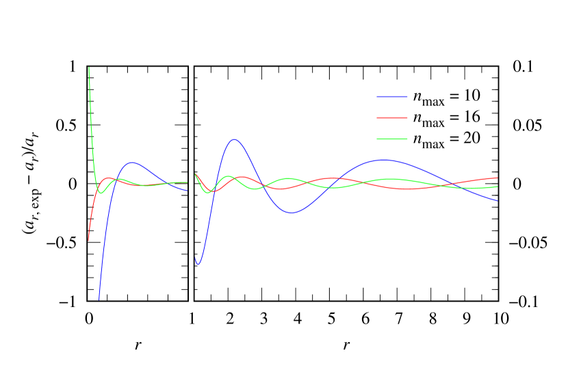
Figure 1: Relative radial-acceleration error of the spherically symmetric NFW halo model as a function of radius. In this plot, $a_{r}$ is the exact acceleration of the NFW halo, while $a_{r,\text{exp}}$ is the radial acceleration derived from the expanded potential using Hernquist–Ostriker’s basis functions with the scale length of $a=6$. The three curves show the effect of the maximum number of the radial expansion terms, $n_{\text{max}}$, on the resulting radial acceleration with the maximum number of the angular expansion terms, $l_{\text{max}}=0$, being retained. Note that the scaling of the abscissa is changed at $r=1$ from the left to the right panel, whereby the ordinate is also re-scaled accordingly.

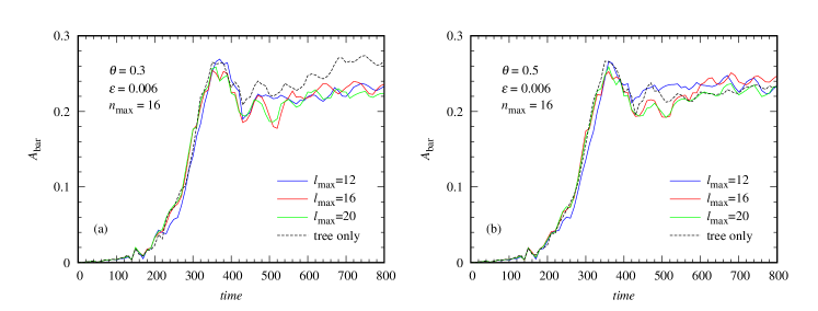
Figure 2: Time evolution of the bar amplitude for $l_{\text{max}}=12,16$, and $20$ obtained using the SCF-FDPS code with the opening angle of $\theta=0.3$ (a), and with that of $\theta=0.5$ (b). For each value of $\theta$, the softening length is $\varepsilon=0.006$, and the maximum number of the radial expansion terms is $n_{\text{max}}=16$. As a reference, the corresponding tree code simulation with $\varepsilon=0.006$ is also plotted for each value of $\theta$.

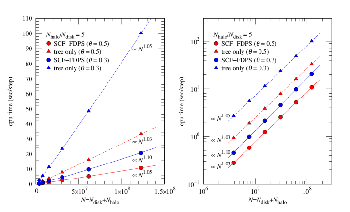
Figure 3: Measured cpu time using 64 cores per step in seconds as a function of the total number of particles, $N=N_{\text{disk}}+N_{\text{halo}}$, where $N_{\text{disk}}$ and $N_{\text{halo}}$ are, respectively, the number of disk particles and that of halo particles with the ratio of $N_{\text{halo}}/N_{\text{disk}}=5$. The left panel shows the cpu time on a linear scale, while the right panel stands for it on a logarithmic scale. The red symbols represent the results for $\theta=0.5$, while the blue symbols denote those for $\theta=0.3$. The circles display the results obtained using the SCF-FDPS code, while the triangles exhibit those using a tree code on which the FDPS library is implemented. The solid and dashed lines with red and blue colors provide power-law fits for corresponding data points.

Figure 4: Fraction of the cpu time occupied by the tree part in the SCF-FDPS code as a function of $N_{\text{disk}}$, which is calculated from the simulations shown in Figure 3.

For the SCF part in the SCF-FDPS code, we need to specify $n_{\text{max}}$ and $l_{\text{max}}$. We determine $n_{\text{max}}$ by comparing the radial acceleration calculated analytically with that derived from the expanded potential of the spherically symmetric NFW halo shown in Equation (18), which is realized by retaining $l_{\text{max}}=0$. In Figure 1, the radial acceleration obtained from the expanded potential for $n_{\text{max}}=10$, $16$, and $20$ is compared with the exact one. The scale length of the basis functions, $a$, is set to be $a=6$. This figure indicates that the radial acceleration obtained with $n_{\text{max}}=10$ shows some relatively large deviation from the exact one, while the radial acceleration with $n_{\text{max}}=16$ is almost comparable to that with $n_{\text{max}}=20$. From this consideration, we adopt $n_{\text{max}}=16$. On the other hand, there is no way to estimate $l_{\text{max}}$ for a spherical halo model. To search for an appropriate value of $l_{\text{max}}$, we carry out convergence tests in which $l_{\text{max}}=12$, $16$, and $20$ are examined with $n_{\text{max}}=16$ being retained. We found that the disk-halo model constructed in Subsection 3.1 forms a bar via the bar instability (see Figure 7). Then, we use the time evolution of the bar amplitude as a measure to determine $l_{\text{max}}$.

Regarding the parameters related to the tree part, we use $\theta=0.3$ and $0.5$ as an opening angle, and $\varepsilon=0.006$ as a softening length of the Plummer type. Gravitational forces are expanded up to quadrupole order.

We assign $N_{\text{disk}}=6{,}400{,}000$ to the disk, and $N_{\text{halo}}=32{,}000{,}000$ to the halo. A time-centered leapfrog algorithm (Press et al., 1986) is employed with a fixed time step of $\Delta t=0.1$.

For comparison, the same disk-halo model is simulated with a tree code on which the FDPS library is implemented. Hereafter, we call this code the FDPS tree code, which is also applied to the SIMD instructions as has been done to the SCF-FDPS code. All the tree parameters are the same as those employed for the convergence tests.

In Figure 2, we show the time evolution of the bar amplitude for $\theta=0.3$ and $0.5$ in each of which $l_{\text{max}}=12,16$, and $20$ are employed, while $n_{\text{max}}=16$ is held fixed. Furthermore, the results with the FDPS tree code are also plotted. On the basis of these results, in particular, paying attention to the behavior of the exponentially growing phase of the bar amplitude from $t=0$ to $t\sim 300$, we select $l_{\text{max}}=16$.

3.3 Performance Tests

We carry out performance tests to examine how fast the SCF-FDPS code is as compared to the FDPS tree code. We measure the cpu time in the cases of $\theta=0.3$ and $0.5$. For each value of $\theta$, the Plummer type softening is used with $\varepsilon=0.006$, and forces are expanded up to quadrupole order. Again, we use a time-centered leap-frog method (Press et al., 1986) with a fixed time step of $\Delta t=0.1$.

In Figure 3, the cpu time using 64 cores per step is plotted as a function of the total number of particles, $N=N_{\text{disk}}+N_{\text{halo}}$, with the ratio of $N_{\text{halo}}/N_{\text{disk}}=5$ being fixed. We can see that the cpu time is nearly proportional to $N$ for both codes, but that the SCF-FDPS code is at least three times faster than the FDPS tree code for $\theta=0.5$, while the former is about five to six times faster than the latter for $\theta=0.3$. As $N_{\text{disk}}$ increases, the ratio of the cpu time measured with the FDPS tree code to that with the SCF-FDPS code decreases for both values of $\theta$. For example, the ratio is 3.3 for $N_{\text{disk}}=640{,}000$, while it is 3.1 for $N_{\text{disk}}=20{,}480{,}000$ when $\theta=0.5$ is used. If $\theta=0.3$ is used, the ratio decreases from 5.9 for $N_{\text{disk}}=640{,}000$ to 4.8 for $N_{\text{disk}}=20{,}480{,}000$. As Figure 4 demonstrates, the fraction of the cpu time exhausted by the tree part in the SCF-FDPS code increases as $N_{\text{disk}}$ increases, while the cpu time consumed by the SCF part is basically proportional to $N_{\text{halo}}$. As a result, that ratio of the cpu time decreases with increasing $N_{\text{disk}}.$

Next, in Figure 5, the cpu time per step is plotted as a function of the number of cores, $N_{\text{core}}$, used on the computer with $N_{\text{disk}}=6{,}400{,}000$ and $N_{\text{halo}}=32{,}000{,}000$ being unchanged. Irrespective of the value of $\theta$, the cpu time scales as $\sim{N_{\text{core}}}^{-0.8}$, which means that the cpu time is almost inversely proportional to $N_{\text{core}}$ for both codes. However, the SCF-FDPS code is about 3.6 times faster than the FDPS tree code for $\theta=0.5$, while the former is approximately 6.4 times faster than the latter for $\theta=0.3$. In the right panel of Figure 5, we can see that as $N_{\text{core}}$ increases, the decrease rate in the cpu time becomes smaller. This is because the cpu clock is made lowered as $N_{\text{core}}$ increases.

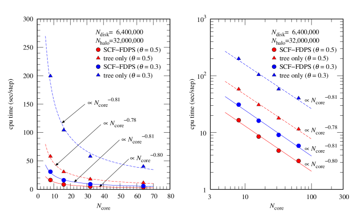
Figure 5: Measured cpu time per step in seconds as a function of the number of cores, $N_{\text{core}}$. The number of disk particles is $N_{\text{disk}}=6{,}400{,}000$, while that of halo particles is $N_{\text{halo}}=32{,}000{,}000$. The meanings of the symbols and those of the solid and dashed lines with red and blue colors are the same as those in Figure 3.

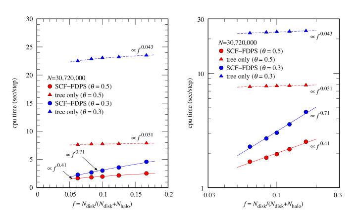
Figure 6: Measured cpu time using 64 cores in seconds per step as a function of the fraction of disk particles, $f=N_{\text{disk}}/(N_{\text{disk}}+N_{\text{halo}})$. The total number of particles is $N=30{,}720{,}000$, and $N_{\text{disk}}$ and $N_{\text{halo}}$ are assigned according to the value of $f$. In this figure, the results with $f=1/16,1/12,1/10,1/8,$ and $1/6$ are plotted. The meanings of the symbols and those of the solid and dashed lines with red and blue colors are the same as those in Figure 3.

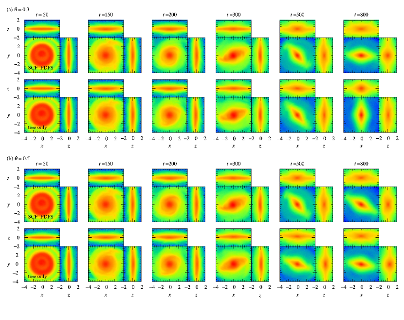
Figure 7: Time evolution of the surface densities of the disk projected on to the $xy$-, $yz$-, and $zx$-planes for the opening angle of $\theta=0.3$ (a), and that of $\theta=0.5$ (b). For each value of $\theta$, the top panels show the results with the SCF-FDPS code, while the bottom panels exhibit those with the tree code into which the FDPS library is implemented. The softening length is set to be $\varepsilon=0.006$ for all simulations. Regarding the SCF-FDPS simulations, $n_{\text{max}}=16$ and $l_{\text{max}}=16$ are used. Note that the drift motion along the vertically upward direction is seen from $t=500$ to $t=800$ for the $\theta=0.5$ simulation with the tree code.

Last, in Figure 6, the cpu time using 64 cores per step is plotted as a function of the fraction of disk particles, $f=N_{\text{disk}}/N$, where $N=N_{\text{disk}}+N_{\text{halo}}$, and we use $f=1/16$, $1/12$, $1/10$, $1/8$, and $1/6$. In this performance test, we change the ratio of $N_{\text{halo}}/N_{\text{disk}}$, while making the total number of particles unchanged as $N=30{,}720{,}000$. As a result, the mass ratio of $M_{\text{halo}}/M_{\text{disk}}$ is not constant but changes identically to the ratio of $N_{\text{halo}}/N_{\text{disk}}$. The other parameters such as $R_{\text{h}}$ and $C_{\text{NFW}}$ are left unchanged. After all, each halo model specified by the value of $f$ is constructed by adjusting the value of $\rho_{0}$ in Equation (19) to the given $M_{\text{halo}}$. Figure 6 indicates how the fraction of the tree part in the SCF-FDPS code affects the cpu time. As a reference, we plot the results using the FDPS tree code. For these tree-code simulations, all particles are obviously calculated with a tree algorithm, so that the cpu time may be expected to be independent of $f$. In reality, the cpu time depends weakly on $f$, and it is proportional to $f^{0.043}$ for $\theta=0.3$, and to $f^{0.031}$ for $\theta=0.5$. On the other hand, the cpu time increases with $f$ if the SCF-FDPS code is used for both values of $\theta$. However, for $\theta=0.5$, the SCF-FDPS code is about 4.5 times faster at $f=1/16$ and about 3.1 times faster at $f=1/6$ than the FDPS tree code, while for $\theta=0.3$, the former is about an order of magnitude faster at $f=1/16$ and about 5.1 times faster at $f=1/6$ than the latter.

3.4 Simulation Results

We carry out simulations of the disk-halo system described by Equations (17) and (18) to examine to what degree the simulation results obtained with the SCF-FDPS code are similar to those with the FDPS tree code. The simulation details are taken over from those adopted for the performance tests. For each value of $\theta$, the energy was conserved to better than 0.028% using the SCF-FDPS code, while it was conserved to better than 0.037% using the FDPS tree code. Figure 7 shows the time evolution of the surface densities of the disk projected on to the $xy$-, $yz$-, and $zx$-planes for $\theta=0.3$ and $0.5$. We find from this figure that the time evolution of the disk surface densities obtained with the SCF-FDPS code is in excellent agreement with that using the FDPS tree code for both values of $\theta$ at least until $t=500$. At later times, owing to the difference in the bar pattern speed from simulation to simulation, the bar phase differs accordingly. Even though a difference in the bar pattern speed is slight at the bar formation epoch, it accumulates with time, so that the difference in the bar phase becomes larger and larger as time progresses. At any rate, the time evolution of the disk is satisfactorily similar between the two codes.

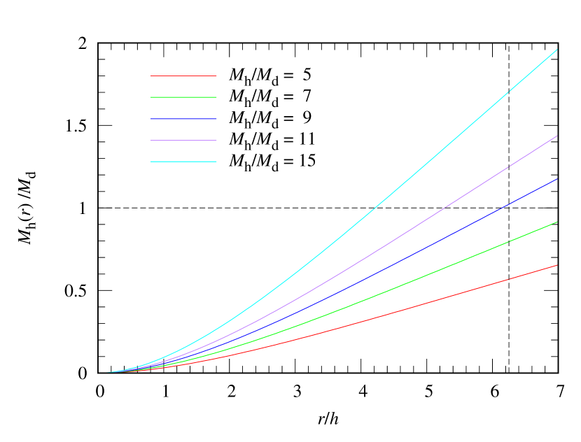
Figure 8: Cumulative mass of each halo used in Figure 6 as a function of radius. The halo masses are normalized by the disk mass, and $M_{\text{h}}=5,7,9,11$, and $15$ correspond to $f=1/6,1/8,1/12$, and $1/16$, respectively, where $f$ is the fraction of disk particles as in Figure 6. The vertical dashed line indicates the radius of 15 kpc when the radial scale length of the disk is assumed to be $h=2.4$ kpc.

4 Discussion

We have shown in Figure 6 that the cpu time taken with the SCF-FDPS code increases as the fraction of $N_{\text{disk}}$ increases. In that figure, the mass of each halo is assigned to that included within $r=30$. However, if the optical edge of the disk is about $15$ kpc, this radius corresponds to $r=6.25$ because the disk scale length is estimated to be $2.4$ kpc (Bland-Hawthorn & Gerhard, 2016). In this case, Figure 8 indicates that the halo mass within $r=6.25$ is at most about 1.7 times the disk mass even for the largest ratio of $M_{\text{h}}/M_{\text{d}}=15$. Since the halo mass within the optical edge of the disk is at least comparable to the disk mass, we may be allowed to regard $f=1/16$ in Figure 6 as a reference value of $f$. Thus, if we are based on the results obtained from the simulations with the value of $f=1/16$ for $\theta=0.3$ and $\theta=0.5$, it follows that in a practical sense, the SCF-FDPS code is about an order of magnitude faster than the FDPS tree code for $\theta=0.3$, and that the former is about 4.5 times faster than the latter for $\theta=0.5$.

We notice from Figure 7(b) that in the simulation for $\theta=0.5$ executed with the FDPS tree code, the disk begins to drift upward along the $z$ axis at $t\sim 300$, which continues to the end of the run, while in the corresponding simulation with the SCF-FDPS code, no upward drift occurs during the run. As found from Figure 7(a), such an upward drift does not arise in the simulation for $\theta=0.3$ with both codes. Thus, in general, tree-code simulations of a disk-halo system do not necessarily lead to a vertical drift motion of the disk. Indeed, in general, linear momentum is not conserved intrinsically in an exact sense for numerical codes based on expansion techniques such as tree and SCF codes. However, our results may suggest that owing to the small fraction of the tree-based calculation, the SCF-FDPS code can easily conserve the linear momentum of each component better than the FDPS tree code to some satisfactory degree.

In our test simulations, we have adopted the softened gravity due to the softening of the Plummer type because it is easily implemented in the SCF-FDPS code. However, in some situations, spline softening (Hernquist & Katz, 1989) may be useful because the force law turns into the pure Newton’s law of universal gravitation at inter-particle distances larger than twice the softening length. Then, we have also implemented the spline softening in the SCF-FDPS code.

For the SCF part in the SCF-FDPS code, we have used Hernquist–Ostriker’s basis set on the ground that it well-describes a cuspy density distribution which the halo model chosen here shows. In addition, we have also implemented Clutton-Brock’s basis set (Clutton-Brock, 1973). This is suitable for cored density distributions, because the lowest order members of the basis functions are based on the Plummer model (Plummer, 1911). Therefore, the SCF-FDPS code can accommodate a wide variety of halo profiles.

In the SCF-FDPS code, disk particles are treated with a tree algorithm, so that the gas component can easily be included by implementing an SPH method (Gingold & Monaghan, 1977; Lucy, 1977), as was done by Hernquist & Katz (1989) who named the code TREESPH. Fortunately, the FDPS library supports the implementation of an SPH method by supplying its sample code. Furthermore, an individual time step method (e.g., McMillan, 1986; Hernquist & Katz, 1989; Makino, 1991) can also be set in the SCF-FDPS code, which enables us, for example, to properly trace particles moving closely around a super-massive black hole residing at the disk center. Accordingly, we will be able to cope with various problems involved in disk galaxies by equipping additional functions such as SPH and individual time step methods with the current SCF-FDPS code.

5 Conclusions

We have developed a fast $N$-body code for simulating disk-halo systems by incorporating an SCF code into a tree code. In particular, the success in achieving the high performance consists in reducing the time-consuming tree-dependent force calculation only to the self-gravity of disk particles by applying an SCF method to the calculation of the gravitational forces between disk and halo particles as well as that of the self-gravity of halo particles. In addition, the SCF-FDPS code has the characteristics that the cpu time is almost proportional to the total number of particles for the fixed number of cores and almost inversely proportional to the number of cores equipped on a computer for the fixed number of particles. As a result, for a disk-halo system, the SCF-FDPS code developed here is at minimum about three times faster and in some case up to an order of magnitude faster, depending on the opening angle, $\theta$, used in the tree method, and on the fraction of tree particles, $f=N_{\text{disk}}/(N_{\text{disk}}+N_{\text{halo}}$), than a highly tuned tree code like the FDPS tree code. Of course, the SCF-FDPS code leads to the time evolution of a disk-halo system similarly to that with the FDPS tree code.

We have implemented Clutton-Brock’s basis set suitable for cored density distributions as well as Hernquist–Ostriker’s basis set appropriate for cuspy density distributions on the SCF-FDPS code, so that it is capable of coping with a wide variety of halo profiles. Furthermore, because the spline softening as well as the Plummer softening have been implemented on that code, it will be able to be applied to the investigation of extensive dynamical problems of disk-halo systems.

We can easily incorporate both SPH and individual time step methods into the tree part in the SCF-FDPS code. Therefore, the SCF-FDPS code will be able to be extended so that we can tackle central issues of disk-galaxy simulations like the evolution of a disk galaxy harboring a central super-massive black hole including a gas component with a huge number of particles by utilizing its high performance.

Appendix A The density and potential basis functions

The basis set adopted here is that constructed by Hernquist & Ostriker (1992). The density and potential basis functions, expressed by $\rho_{nlm}(\bm{r})$ and $\Phi_{nlm}(\bm{r})$, respectively, are represented by

$$\rho_{nlm}(\textbf{{r}})=K_{nl}\frac{M}{2\pi a^{3}}\frac{(r/a)^{l}}{(r/a){(1+r/a)}^{2l+3}}C_{n}^{(2l+3/2)}(\xi)\sqrt{4\pi}\,Y_{lm}(\theta,\,\phi)$$ (A1)

and

$$\Phi_{nlm}(\textbf{{r}})=-\frac{GM}{a}\frac{(r/a)^{l}}{(1+r/a)^{2l+1}}C_{n}^{(2l+3/2)}(\xi)\sqrt{4\pi}\,Y_{lm}(\theta,\,\phi),$$ (A2)

where $M$ is the mass of the system, $a$ is the scale length, $C_{n}^{(\alpha)}(\xi)$ are the ultraspherical, or Gegenbauer polynomials (Abramowitz & Stegun, 1972) with $\xi$ being the radial transformation defined by

$$\xi=\frac{r-a}{r+a},$$ (A3)

and $Y_{lm}(\theta,\,\phi)$ are spherical harmonics which are related to associated Legendre polynomials, $P_{lm}(x)$, by

$$Y_{lm}(\theta,\,\phi)=\sqrt{\frac{2l+1}{4\pi}\frac{(l-m)!}{(l+m)!}}\,P_{lm}(\cos\theta)\exp(im\phi),$$ (A4)

where $i$ is the imaginary unit.

In Equation (A1), the normalization factor, $K_{nl}$, is provided by

$$K_{nl}=\frac{1}{2}n(n+4l+3)+(l+1)(2l+1).$$ (A5)

References

- Abramowitz & Stegun (1972) Abramowitz, M., & Stegun, I. A. 1972, Handbook of Mathematical Functions with Formulas, Graphs, and Mathematical Tables (New York: Dover), 774
- Athanassoula (2002) Athanassoula, E. 2002, ApJ, 569, L83, doi: 10.1086/340784
- Barnes & Hut (1986) Barnes, J., & Hut, P. 1986, Nature, 324, 446, doi: 10.1038/324446a0
- Bédorf et al. (2012) Bédorf, J., Gaburov, E., & Portegies Zwart, S. 2012, Journal of Computational Physics, 231, 2825, doi: 10.1016/j.jcp.2011.12.024
- Bland-Hawthorn & Gerhard (2016) Bland-Hawthorn, J., & Gerhard, O. 2016, ARA&A, 54, 529, doi: 10.1146/annurev-astro-081915-023441
- Clutton-Brock (1973) Clutton-Brock, M. 1973, Ap&SS, 23, 55, doi: 10.1007/BF00647652
- D’Onghia et al. (2013) D’Onghia, E., Vogelsberger, M., & Hernquist, L. 2013, ApJ, 766, 34, doi: 10.1088/0004-637X/766/1/34
- Dubinski et al. (2009) Dubinski, J., Berentzen, I., & Shlosman, I. 2009, ApJ, 697, 293, doi: 10.1088/0004-637X/697/1/293
- Fujii et al. (2011) Fujii, M. S., Baba, J., Saitoh, T. R., et al. 2011, ApJ, 730, 109, doi: 10.1088/0004-637X/730/2/109
- Fujii et al. (2018) Fujii, M. S., Bédorf, J., Baba, J., & Portegies Zwart, S. 2018, MNRAS, 477, 1451, doi: 10.1093/mnras/sty711
- Fujii et al. (2019) —. 2019, MNRAS, 482, 1983, doi: 10.1093/mnras/sty2747
- Gingold & Monaghan (1977) Gingold, R. A., & Monaghan, J. J. 1977, MNRAS, 181, 375, doi: 10.1093/mnras/181.3.375
- Hernquist (1990) Hernquist, L. 1990, ApJ, 356, 359, doi: 10.1086/168845
- Hernquist & Katz (1989) Hernquist, L., & Katz, N. 1989, ApJS, 70, 419, doi: 10.1086/191344
- Hernquist & Ostriker (1992) Hernquist, L., & Ostriker, J. P. 1992, ApJ, 386, 375, doi: 10.1086/171025
- Hernquist et al. (1995) Hernquist, L., Sigurdsson, S., & Bryan, G. L. 1995, ApJ, 446, 717, doi: 10.1086/175829
- Hozumi et al. (2023) Hozumi, S., Nitadori, K., & Iwasawa, M. 2023, SCF-FDPS, v0.0.1-20230213, Zenodo, doi: 10.5281/zenodo.7633122
- Iwasawa et al. (2016) Iwasawa, M., Tanikawa, A., Hosono, N., et al. 2016, PASJ, 68, 54, doi: 10.1093/pasj/psw053
- Lucy (1977) Lucy, L. B. 1977, AJ, 82, 1013, doi: 10.1086/112164
- Makino (1991) Makino, J. 1991, PASJ, 43, 859
- McMillan (1986) McMillan, S. L. W. 1986, in Lecture Notes in Physics, Vol. 267, The Use of Supercomputers in Stellar Dynamics, ed. P. Hut & S. L. W. McMillan (Berlin: Springer), 156, doi: 10.1007/BFb0116406
- Miki & Umemura (2018) Miki, Y., & Umemura, M. 2018, MNRAS, 475, 2269, doi: 10.1093/mnras/stx3327
- Namekata et al. (2018) Namekata, D., Iwasawa, M., Nitadori, K., et al. 2018, PASJ, 70, 70, doi: 10.1093/pasj/psy062
- Navarro et al. (1996) Navarro, J. F., Frenk, C. S., & White, S. D. M. 1996, ApJ, 462, 563, doi: 10.1086/177173
- Navarro et al. (1997) —. 1997, ApJ, 490, 493, doi: 10.1086/304888
- Plummer (1911) Plummer, H. C. 1911, MNRAS, 71, 460, doi: 10.1093/mnras/71.5.460
- Press et al. (1986) Press, W. H., Flannery, B. P., Teukolsky, S. A., & Vetterling, W. T. 1986, Numerical Recipes: The Art of Scientific Computing (Cambridge: Cambridge Univ. Press)
- Sofue & Rubin (2001) Sofue, Y., & Rubin, V. 2001, ARA&A, 39, 137, doi: 10.1146/annurev.astro.39.1.137
- Toomre (1964) Toomre, A. 1964, ApJ, 139, 1217, doi: 10.1086/147861
- Vine & Sigurdsson (1998) Vine, S., & Sigurdsson, S. 1998, MNRAS, 295, 475, doi: 10.1046/j.1365-8711.1998.01325.x
- Zang & Hohl (1978) Zang, T. A., & Hohl, F. 1978, ApJ, 226, 521, doi: 10.1086/156636