A Semantics for Counterfactuals
in Quantum Causal Models

Abstract

We introduce a formalism for the evaluation of counterfactual queries in the framework of quantum causal models, by generalising the three-step procedure of abduction, action, and prediction in Pearl’s classical formalism of counterfactuals [1]. To this end, we define a suitable extension of Pearl’s notion of a ‘classical structural causal model’, which we denote analogously by ‘quantum structural causal model’. We show that every classical (probabilistic) structural causal model can be extended to a quantum structural causal model, and prove that counterfactual queries that can be formulated within a classical structural causal model agree with their corresponding queries in the quantum extension – but the latter is more expressive. Counterfactuals in quantum causal models come in different forms: we distinguish between active and passive counterfactual queries, depending on whether or not an intervention is to be performed in the action step. This is in contrast to the classical case, where counterfactuals are always interpreted in the active sense. As a consequence of this distinction, we observe that quantum causal models break the connection between causal and counterfactual dependence that exists in the classical case: (passive) quantum counterfactuals allow counterfactual dependence without causal dependence. This illuminates an important distinction between classical and quantum causal models, which underlies the fact that the latter can reproduce quantum correlations that violate Bell inequalities while being faithful to the relativistic causal structure.

1 Introduction

The world of alternative possibilities has been pondered upon and analyzed routinely, in many fields of study including but not limited to social [2] and public policy [3], psychiatry [4], economy [5], weather and climate change [6], artificial intelligence [7], philosophy and causality [8, 9]. For example, questions involving counterfactuals can have important social and legal implications, such as “Given that the patient has died after treatment, would they have survived had they been given a different treatment?”

The status of counterfactual questions also figures centrally in debates about quantum mechanics [10], where results such as Bell’s theorem [11] and the Kochen-Specker theorem [12] have been interpreted as requiring the abandonment of “counterfactual definiteness”, encapsulated in Peres’ famous dictum “unperformed experiments have no results” [13]. So can this assertion be used by a lawyer as an argument to dismiss a medical malpractice lawsuit as meaningless? Presumably not. Since the world is fundamentally quantum, dismissing all counterfactual questions as meaningless in quantum theory seems too strong. Here, we seek to delineate what questions can be unambiguously answered when unambiguously formulated, and to provide some direction for resolving the ambiguity that is inherent in counterfactual questions that are not so carefully constructed.

The semantics of counterfactuals has a controversial history. One of the early accounts is due to David Lewis [14]. He proposed to evaluate counterfactuals by a similarity analysis of possible worlds, where “a counterfactual ‘If it were that A, then it would be that C’ is (non-vacuously) true if and only if some (accessible) world where both A and C are true is more similar to our actual world, overall, than is any world where A is true but C is false” [14]. This analysis is inevitably vague, as it requires an account of “similarity” among possible worlds, which Lewis attempts to resolve via a system of priorities. The goal is to identify closest worlds as possible worlds in which things are kept more or less the same as in our actual world, except for some ‘minimal changes’, required to make the antecedent of a given counterfactual true.

A recent approach, due to Judea Pearl, proposes to define counterfactuals in terms of a sufficiently well-specified causal model for a given situation, denoted by a (classical) structural causal model [1]. In Pearl’s approach, the ‘minimal changes’ required to make the antecedent of a counterfactual true are conceptualised in terms of an intervention, which breaks the causal connections into the variable being intervened upon while fixing it to the required counterfactual value. Structural causal models feature at the top of a hierarchy of progressively sophisticated models that can answer progressively sophisticated questions, which Pearl has dubbed the “ladder of causation” [15] (see Fig. 1).

As is well known, however, the classical causal model-framework of Pearl fails to reproduce quantum correlations, while maintaining faithfulness to the relativistic causal structure—as vividly expressed by Bell’s theorem [11] and recent ‘fine-tuning theorems’ [16, 17, 18]. The program of quantum causal models aims to extend the classical causal model-framework, while maintaining compatibility with relativistic causality. One of the aims of our work is to complete the last rung in the quantum analogue of Pearl’s “ladder of causation”, by proposing a framework to answer counterfactual queries in quantum causal models.

A key distinction from the classical case is that, due to the indeterminism inherent in quantum causal models, counterfactual queries do not always have truth values (unlike in Lewis’ and Pearl’s accounts). Another difference is that an intervention is not always required in order to make the antecedent of a counterfactual true. This leads to a richer semantics for counterfactual in the quantum case, which contains Pearl’s classical structural causal model as a special case, as we show.

Finally, an important distinction regards the connection between counterfactual dependence and causal dependence. In Pearl’s account, counterfactual dependence requires causal dependence. Following an informal definition by David Hume proposed an analysis of causal dependence starting from his notion of counterfactual dependence. In contrast, in quantum causal models there can be counterfactual dependence among events without causal dependence. This fact sheds new light on the nature of the compatibility with relativistic causality that is offered by quantum causal models.

The rest of the paper is organised as follows. In Sec. 2, we review the basic ingredients to Pearl’s ladder of causation (see Fig. 1), as well as his three-step procedure for evaluating counterfactuals based on the notion of (classical) structural causal models. In Sec. 3, we highlight the issues in accommodating quantum theory within this framework, in the light of Bell’s theorem and the assumption of “no fine-tuning” [16, 17]. The framework of quantum causal models aims to resolve this discrepancy. We introduce some key notions and notation of the latter in Sec. 4, which will set the stage for our definition of quantum counterfactuals and their semantics based on a novel notion of quantum structural causal models in Sec. 5. In Sec. 6, we show that Pearl’s classical formalism of counterfactuals naturally embeds into our framework; conversely, in Sec. 7 we elaborate on how our framework generalizes Pearl’s formalism, by distinguishing passive from active counterfactuals in quantum causal models. This results in a difference between causal and counterfactual dependence in quantum causal models, which pinpoints a remarkable departure from classical counterfactual reasoning, and is discussed using the pertinent example of the Bell scenario in Sec. 7.3. Sec. 8 reflects on some of the key assumptions to our notion of quantum counterfactuals in the context of recent developments on quantum statistical inference. Sec. 9 concludes.

2 The Classical Causal Model Framework

This section contains the minimal background on classical causal models and the evaluation of counterfactuals, required for the generalization to the quantum case in Sec. 5. We will review a modest fraction of the framework outlined in much more detail in Ref. [1]; readers familiar with the latter may readily skip this section.

In his book on causality [1], Judea Pearl identifies a hierarchy of progressively sophisticated models that are capable of answering progressively sophisticated causal queries. This hierarchy is often depicted as the three-step ‘Ladder of Causation’, with different rungs corresponding to the different levels of causal queries (see Fig. 1).

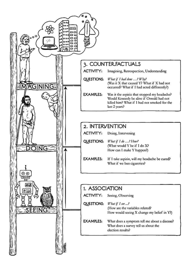
Figure 1: A depiction of “The Ladder of Causation”. [Republished with permission from Ref. [15].]

At the bottom of the ladder is the level of association (‘level 1’), related to observations and statistical relations. It answers questions such as “how would seeing $X$ change my belief in $Y$?” The second rung is the level of intervention (‘level 2’), which considers questions such as “If I take aspirin, will my headache be cured”? Levels 1 and 2 are related to Bayesian networks and causal Bayesian networks, respectively, and we will formally define these in the coming subsections. The final rung in the ladder of causation is the level of counterfactuals (‘level 3’), associated with activities such as imagining, retrospecting, and understanding. It considers questions such as “Was it the aspirin that stopped my headache?”, “Had I not taken the aspirin, would my headache not have been cured?” etc. In other words, counterfactuals deal with ‘why’-questions.

Pearl argues that the levels of intervention and counterfactuals are particularly important for human intelligence and understanding, as they are crucial for our internal modeling of the world and the effects of our actions. In contrast, he argues that current artificial intelligence (AI)—however impressive— is still restricted to level 1 of the hierarchy. Considering the coming age of quantum computation, one of the motivations of our work is to extend Pearl’s analysis to the framework of quantum causal models, which may have applications for future quantum AI.

2.1 Level 1 - Bayesian networks

In Pearl’s framework, level 1 of the ladder of causation (Fig. 1) is the level of association, which encodes statistical data in the form of a probability distribution $P(\mathbf{v})=P(v_{1},\cdots,v_{n})$ over random variables $\mathbf{V}=\{V_{i}\}_{i=1}^{n}$. The latter are assumed to take values in a finite set, whose elements are denoted by the corresponding lowercase letters $v_{i}$’s. The proposition ‘$V_{i}=v_{i}$’ describes the event where the random variable $V_{i}$ takes the value $v_{i}$, and $P(v_{i}):=P(V_{i}=v_{i})$ denotes the probability that this event occurs.

Statistical independence conditions in a probability distribution can be conveniently represented graphically using directed acyclic graphs (DAGs), which in this context are also known as Bayesian networks. The nodes in a Bayesian network $G$ represent the random variables $\mathbf{V}=\{V_{i}\}_{i=1}^{n}$, while arrows (‘$V_{j}\rightarrow V_{k}$’) in $G$ impose a ‘kinship’ relation: we call $\mathrm{Pa}(V_{i})=\mathrm{Pa}_{i}:=\{V_{j}\in\mathbf{V}\mid(V_{j}\rightarrow V_{i})\in G\}$ the “parents” and $\mathrm{Ch}(V_{i})=\mathrm{Ch}_{i}:=\{V_{j}\in\mathbf{V}\mid(V_{i}\rightarrow V_{j})\in G\}$ denotes the “children” of the node $V_{i}$. For example, in Fig. 2, $V_{1}$ is the parent node of $V_{2}$ and $V_{3}$; $V_{4}$ is a child node of $V_{2}$, $V_{3}$ and $V_{6}$.

Figure 2: A directed acyclic graph (DAG) with nodes $\mathbf{V}=\{V_{1},\cdots,V_{6}\}$ representing random variables, and arrows representing (causal) statistical dependencies.

Definition 1 (Classical Markov condition).

A joint probability distribution $P(\mathbf{v})=P(v_{1},\cdots,v_{n})$ is said to be Markov relative to a DAG $G$ with nodes $\mathbf{V}=\{V_{i}\}_{i=1}^{n}$ if and only if there exist conditional probability distributions $P(v_{i}|pa_{i})$ for each $V_{i}\in\mathbf{V}$ such that,

$$P(\mathbf{v})=\prod_{i=1}^{n}P(v_{i}|pa_{i})\;.$$ (1)

In general, a probability distribution will be Markov relative to different Bayesian networks, corresponding to different ways it can be decomposed into conditional distributions. Moreover, a Bayesian network will have many distributions which are Markov with respect to it. Note that at this level (level 1), the DAG $G$ representing a Bayesian network does not carry causal meaning, but is merely a convenient representation of statistical conditional independences.

2.2 Level 2 - Causal Bayesian networks and classical causal models

At level 2 of the hierarchy are causal (Bayesian) networks. In contrast to Bayesian networks, the arrows between nodes $\mathbf{V}=\{V_{i}\}^{n}_{i=1}$ in a causal Bayesian network do encode causal relationships. In particular, the parents $\mathrm{Pa}(V_{i})$ of a node $V_{i}$ are now interpreted as direct causes of $V_{i}$.

Definition 2 (Classical Causal Model).

A classical causal model is a pair $\langle G,P\rangle$, consisting of a directed acyclic graph $G$ encoding a causal Bayesian network, and a probability distribution $P$ that is Markov with respect to $G$, according to Def. 1.

Moreover, a causal network is an oracle for interventions. The effect of an intervention is modeled as a “mini-surgery” in the graph that cuts all incoming arrows into the node being intervened upon and sets it to a specified value. What is more, given a classical causal model $\langle G,P\rangle$, we define the do-intervention $\mathrm{do}(\mathbf{X}=\mathbf{x})$ on a subset of nodes $\mathbf{X}\subset\mathbf{V}$ as the submodel $\langle G_{\mathbf{x}},P_{\mathbf{x}}\rangle$, where $G_{\mathbf{x}}$ is the modified DAG with the same nodes as $G$, but with all incoming arrows $V_{j}\rightarrow V_{i}$ for $V_{i}\in\mathbf{X}$ removed from $G$, and where $P_{\mathbf{x}}$ arises from $P$ by setting the values at $\mathbf{X}$ to $\mathbf{x}$. More precisely, letting $\mathbf{V}_{\mathbf{x}}=\mathbf{V}\backslash\mathbf{X}$

$$P_{\mathbf{x}}(\mathbf{v})=\prod_{V_{i}\in\mathbf{X}}\delta_{v_{i},x_{i}}\prod_{V_{i}\in\mathbf{V}_{\mathbf{x}}}P(v_{i}|pa_{i})\;.$$ (2)

For example, if we perform a do-intervention $\mathrm{do}(V_{2}=v_{2})$ on the classical causal model $\langle G,P\rangle$ with DAG $G$ in Fig. 2, then $G_{v_{2}}$ is the DAG shown in Fig. 3, and the truncated factorization formula for the remaining variables reads

$$P_{v_{2}}(v_{1},v_{3},v_{4},v_{5},v_{6})=P(v_{1})P(v_{3}|v_{1})P(v_{4}|V_{2}=v_{2},v_{3},v_{6})P(v_{5}|v_{4})P(v_{6})\;.$$ (3)

Figure 3: The directed acyclic graph from Fig. 2 after a do-intervention on node $V_{2}$. The effect of this do-intervention is graphically represented by removing all the arrows into $V_{2}$.

2.3 Level 3 - Structural causal models and the evaluation of counterfactuals

At level 3 of the hierarchy are (classical) structural causal models. Such models consist of a set of nodes $(\mathbf{V},\mathbf{U})$, distinguished into endogenous variables $\mathbf{V}$ and exogenous variables $\mathbf{U}$, together with a set of functions $\mathbf{F}$ that encode structural relations between the variables. The term “exogenous” indicates that any causes of such variables lie outside the model; they can be thought of as local ‘noise variables’.

Definition 3 (Classical Structural Causal Model).

A (classical) structural causal model (CSM) $M$ is a triple $M=\langle\mathbf{U},\mathbf{V},\mathbf{F}\rangle$, where $\mathbf{V}=\{V_{1},\dots,V_{n}\}$ is a set of endogenous random variables, $\mathbf{U}=\{U_{1},\cdots,U_{n}\}$ is a set of exogenous random variables and $\mathbf{F}=\{f_{1},\dots,f_{n}\}$ is a set of functions of the form $f_{i}:U_{i}\times\mathrm{Pa}_{i}\rightarrow V_{i}$, where $\mathrm{Pa}_{i}:=\{V_{j}\in\mathbf{V}\mid V_{j}\subset f^{-1}_{i}(V_{i})\}\subset\mathbf{V}$.

Every structural causal model $M$ is associated with a directed graph $G(M)$, which represents the causal structure of the model as specified by the relations $G(M)\ni(V_{j}\stackrel{{\scriptstyle f_{i}}}{{\rightarrow}}V_{i})\Leftrightarrow V_{j}\in\mathrm{Pa}_{i}$. Here, we will restrict CSMs to those defining directed acyclic graphs. For example, the causal model of Fig. 2 can be extended to a CSM with causal relations as depicted in Fig. 4.

Figure 4: A classical structural causal model (CSM) with endogenous nodes $\mathbf{V}=\{V_{1},\cdots,V_{6}\}$ and exogenous nodes $\mathbf{U}=\{U_{1},\cdots,U_{6}\}$.

In analogy with the do-interventions for causal Bayesian networks in Sec. 2.2, we define do-interventions in a CSM $M=\langle\mathbf{U},\mathbf{V},\mathbf{F}\rangle$. Let $\mathbf{X}\subset\mathbf{V}$ with corresponding exogenous variables $\mathbf{U}(\mathbf{X})\subset\mathbf{U}$ and functions $\mathbf{F}(\mathbf{X})\subset\mathbf{F}$, and let $\mathbf{V}_{\mathbf{x}}=\mathbf{V}\backslash\mathbf{X}$, $\mathbf{U}_{\mathbf{x}}=\mathbf{U}\backslash\mathbf{U}(\mathbf{X})$ and $\mathbf{F}_{\mathbf{x}}=\mathbf{F}\backslash\mathbf{F}(\mathbf{X})$. Then the do-intervention $\mathrm{do}(\mathbf{X}=\mathbf{x})$ defines a submodel $M_{\mathbf{x}}=\langle\mathbf{U}_{\mathbf{x}},(\mathbf{V}_{\mathbf{x}},\mathbf{X}=\mathbf{x}),\mathbf{F}_{\mathbf{x}}\rangle$. In terms of the causal graph $G(M)$, the action $\mathrm{do}(\mathbf{X}=\mathbf{x})$ removes all incoming arrows to the nodes $X_{i}$, thus generating a new graph $G(M_{\mathbf{x}})$.

The submodel $M_{\mathbf{x}}$ represents a minimal change to the original model $M$ such that $\mathbf{X}=\mathbf{x}$ is true while keeping the values of the exogenous variables fixed – which are thought of as “background conditions”. In turn, we can use $M_{\mathbf{x}}$ to analyze counterfactual statements with antecedent $\mathbf{X}=\mathbf{x}$.

Definition 4 (Counterfactual).

Let $M=\langle\mathbf{U},\mathbf{V},\mathbf{F}\rangle$ be a structural causal model, and let $\mathbf{X},\mathbf{Y}\subseteq\mathbf{V}$. The counterfactual statement “$\mathbf{Y}$ would have been $\mathbf{y}$, had $\mathbf{X}$ been $\mathbf{x}$, in a situation specified by the background variables $\mathbf{U}=\mathbf{u}$” is denoted by $\mathbf{Y}_{\mathbf{x}}(\mathbf{u})=\mathbf{y}$, where $\mathbf{Y}_{\mathbf{x}}(\mathbf{u})$ is the potential response of $\mathbf{Y}$ to the action $\mathrm{do}(\mathbf{X}=\mathbf{x})$, that is, the solution for $\mathbf{Y}$ of the modified set of equations $\mathbf{F}_{\mathbf{x}}$ in the submodel $M_{\mathbf{x}}$. $\mathbf{X}=\mathbf{x}$ is called the antecedent and $\mathbf{Y}=\mathbf{y}$ is the consequent of the counterfactual.

Note that given any complete specification $\mathbf{U}=\mathbf{u}$ of the exogenous variables, every counterfactual statement of the form above has a truth value. Denoting a “causal world” by the pair $\langle M,\mathbf{u}\rangle$, we can say that a counterfactual has a truth value in every causal world where it can be defined. This is the case even when the background variables determine $\mathbf{X}$ to have a value different from the value specified in the antecedent since the counterfactual is evaluated relative to the modified submodel $M_{\mathbf{x}}$.

Definition 5 (Probabilistic structural causal model).

A probabilistic structural causal model (PSM) is defined by a pair $\langle M,P(\mathbf{u})\rangle$, where $M=\langle\mathbf{V},\mathbf{U},\mathbf{F}\rangle$ is a structural causal model (see Def  3) and $P(\mathbf{u})$ is a probability distribution defined over the exogenous variables $\mathbf{U}$ of $M$.

Since every endogenous variable $V_{i}\in\mathbf{V}$ is a function of $U_{i}$ and its parent nodes, $f_{i}:U_{i}\times\mathrm{Pa}_{i}\rightarrow V_{i}$, the distribution $P(\mathbf{u})$ in a PSM $\langle M,P(\mathbf{u})\rangle$ defines a probability distribution over every subset $\mathbf{Y}\subseteq\mathbf{V}$ by

$$P(\mathbf{y}):=P(\mathbf{Y}=\mathbf{y})=\sum_{\mathbf{u}|\mathbf{Y}(\mathbf{u})=\mathbf{y}}P(\mathbf{u})\;.$$ (4)

In particular, the probability of the counterfactual “$\mathbf{Y}$ would have been $\mathbf{y}$, had $\mathbf{X}$ been $\mathbf{x}$, given $\mathbf{U}$ is $\mathbf{u}$” can be computed using the submodel $M_{\mathbf{x}}$ as

$$P(\mathbf{Y}_{\mathbf{x}}=\mathbf{y})=\sum_{\mathbf{u}|\mathbf{Y}_{\mathbf{x}}(\mathbf{u})=\mathbf{y}}P(\mathbf{u})\;.$$ (5)

More generally, the probability of a counterfactual query might be conditioned on prior observations ‘$\mathbf{e}$’. In this case, we first update the probability distribution $P(\mathbf{u})$ in the PSM to obtain a modified probability distribution $P(\mathbf{u}\mid\mathbf{e})$ conditioned on observed data $\mathbf{e}$ and then use this updated probability distribution to evaluate the probability for the counterfactual as in Eq. (5). Combining the above steps, one arrives at the following theorem, proved in Ref. [1]:

Theorem 1 (Pearl [1]).

Given a probabilistic structural causal model (PSM) $\langle M,P(\mathbf{u})\rangle$ (see Def  5), and subsets $\mathbf{X},\mathbf{Y},\mathbf{E}\subset\mathbf{V}$, the probability for the counterfactual “would $\mathbf{Y}=\mathbf{y}$, had $\mathbf{X}=\mathbf{x}$, given that $\mathbf{E}=\mathbf{e}$”, is denoted by $P(\mathbf{Y}_{\mathbf{x}}|\mathbf{e})$ and can be evaluated systematically by a three-step procedure:

• Step 1: Abduction: using the observed data $\mathbf{E}=\mathbf{e}$, use Bayesian inference to update the probability distribution $P(\mathbf{u})$ corresponding to the PSM $\langle M,P(\mathbf{u})\rangle$ to obtain $P(\mathbf{u}|\mathbf{e})$.

• Step 2: Action: perform a do-intervention $\mathrm{do}(\mathbf{X}=\mathbf{x})$, by which the values of $\mathbf{X}\subset\mathbf{V}$ are specified independent of their parent nodes. The resultant model is denoted as $M_{\mathbf{x}}$.

• Step 3: Prediction: in the modified model $\langle M_{\mathbf{x}},P(\mathbf{u}|\mathbf{e})\rangle$, compute the probability of $\mathbf{Y}$ as by Eq. (5).

As an example, consider the situation where $\mathbf{X}=\mathbf{x}$ and $\mathbf{Y}=\mathbf{y}$ are observed, that is, $\mathbf{E}=(\mathbf{X},\mathbf{Y})$. We evaluate the probability of the counterfactual “$\mathbf{Y}$ would have been equal to $\mathbf{y}^{\prime}$ had $\mathbf{X}$ been $\mathbf{x}^{\prime}$” as:

$$P(\mathbf{Y}_{\mathbf{x}^{\prime}}=\mathbf{y}^{\prime}|\mathbf{X}=\mathbf{x},\mathbf{Y}=\mathbf{y}) =\sum_{\mathbf{u}|\mathbf{Y}_{\mathbf{x}^{\prime}}(\mathbf{u})=\mathbf{y}^{\prime}}P(\mathbf{u}|\mathbf{X}=\mathbf{x},\mathbf{Y}=\mathbf{y})=\sum_{\mathbf{u}|\mathbf{Y}_{\mathbf{x}^{\prime}}(\mathbf{u})=\mathbf{y}^{\prime}}\frac{P(\mathbf{X}=\mathbf{x},\mathbf{Y}=\mathbf{y}|\mathbf{u})P(\mathbf{u})}{P(\mathbf{X}=\mathbf{x},\mathbf{Y}=\mathbf{y})}\;,$$ (6)

where we used Eq. (5) in the first and Bayes’ theorem in the second step.

In temporal metaphors, step 1 explains the past (the exogenous variables $\mathbf{U}$) in light of the current evidence $\mathbf{e}$; step 2 minimally bends the course of history to comply with the hypothetical antecedent and step 3 predicts the future based on our new understanding of the past and our newly established condition.

3 Quantum violations of classical causality

Classical causal models face notorious difficulties in explaining quantum correlations. Firstly, Bell’s theorem [11, 20, 21] can be interpreted in terms of classical causal models, thus proving that such models cannot reproduce quantum correlations (in particular, those that violate a Bell inequality) while maintaining relativistic causal structure and the assumption of “free choice”. The latter is the assumption that experimentally controllable parameters like measurement settings can always be chosen via “free variables”, which can be understood as variables that have no relevant causes in a causal model for the experiment. That is, they share no common causes with, nor are caused by, any other variables in the model. Thus, “free variables” can be modeled as exogenous variables.

For concreteness, consider the standard Bell scenario with a causal structure represented in the DAG in Fig. 5, where variables $A$ and $B$ denote the outcomes of experiments performed by two agents, Alice and Bob. Variables $X$ and $Y$ denote their choices of experiment, which are assumed to be “free variables” and thus have no incoming arrows. Since Alice and Bob perform measurements in space-like separated regions, no relativistic causal connection is allowed between $X$ and $B$ nor between $Y$ and $A$. In this scenario, Reichenbach’s principle of common cause [22, 23] – which is a consequence of the classical causal Markov condition – implies the existence of common causes underlying any correlations between the two sides of the experiment. $\Lambda$ denotes a complete specification of any such common causes. As we are assuming a relativistic causal structure, those must be in the common past light cone of Alice’s and Bob’s experiments.

Figure 5: A Directed Acyclic Graph (DAG) depicting the standard Bell scenario.

Marginalizing over the common cause variable $\Lambda$, the causal Markov condition applied to the DAG in Fig. 5 implies the factorization:

$$P(AB|XY)=\sum_{\Lambda}P(\Lambda)P(A|X\Lambda)P(B|Y\Lambda)\;.$$ (8)

A model satisfying Eq. (8) is also called local hidden variable model. Importantly, local hidden variable models satisfy the Bell inequalities [11, 20], which have been experimentally violated by quantum correlations [24, 25, 26, 27]. It follows that no classical causal model can explain quantum correlations under the above assumptions.

More recently, Wood and Spekkens [16] showed that certain Bell inequality violations cannot be reproduced by any classical causal model that satisfies the assumption of “no fine-tuning”. This is the requirement that any conditional independence between variables in the model be explained as arising from the structure of the causal graph, rather than from fine-tuned model parameters. This assumption is essential for causal discovery – without it, it is generally not possible to experimentally determine which of a number of candidate graphs faithfully represents a given situation. This result was later generalized to arbitrary Bell and Kochen-Specker inequality violations in Refs. [17, 18].

These results motivate the search for a generalization of classical causal models that accommodates quantum correlations and allows for causal discovery, while maintaining faithfulness to relativistic causal structure. Ref. [23] considers modifications of Reichenbach’s principle of common cause [22]—which is implied by the causal Markov condition in the special case of the common cause scenario in Fig. 5, as assumed in Bell’s theorem [11, 20]. The authors of Ref. [23] argue that one could maintain the principle of common cause—the requirement that correlations between two causally disconnected events should be explained via common causes—by relaxing the condition that a full specification of those common causes factorizes the probabilities for the events in question, as by Eq. (8). Using the Leifer-Spekkens formalism for quantum conditional states, they instead propose that Eq. (8) should be replaced by the requirement that the channels between the common cause and Alice and Bob’s labs factorize—or more precisely, the Choi-Jamiołkowski operators corresponding to those channels. This is essentially the type of resolution of Bell’s theorem that is provided by quantum causal models, to which we now turn. After introducing structural quantum causal models in Sec. 4.1 and quantum counterfactuals queries in Sec. 5, in Sec. 7.3 we will revisit the Bell scenario from the perspective of counterfactuals in quantum causal models.

4 Quantum causal models

In recent years a growing number of papers have addressed the problem of generalizing the classical causal model formalism to accommodate quantum correlations, in a way that is compatible with relativistic causality and faithfulness. This has led to the development of various frameworks for quantum causal models. The more developed of those are the frameworks by Costa and Shrapnel [28] and Barrett, Lorenz and Oreshkov [29]. In this work, we use a combination of the notation and features of both of these formalisms.

Quantum nodes and quantum interventions. Recall that in a classical causal model, a node represents a locus for potential interventions. In order to generalize this to the quantum case, we start by introducing a quantum node $A$, which is associated with two Hilbert spaces $\mathcal{H}_{A^{\mathrm{in}}}$ and $\mathcal{H}_{A^{\mathrm{out}}}$, corresponding to the incoming system and the outgoing system, respectively. An intervention at a quantum node $A$ is represented by a quantum instrument $\mathcal{I}^{z}_{A}$ (see Fig. 6). This is a set of trace-non-increasing completely positive (CP) maps from the space of linear operators on $\mathcal{H}_{A^{\mathrm{in}}}$ to the space of linear operators on $\mathcal{H}_{A^{\mathrm{out}}}$,

$$\mathcal{I}_{A}^{z}=\{\mathcal{M}_{A}^{a|z}:\mathcal{L}({\mathcal{H}_{A^{\mathrm{in}}}})\rightarrow\mathcal{L}({\mathcal{H}_{A^{\mathrm{out}}}})\}_{a}\;,$$ (9)

such that $\mathcal{M}_{A}=\sum_{a}\mathcal{M}_{A}^{a|z}$ is a completely positive, trace-preserving (CPTP) map—i.e. a quantum channel. Here, $z$ is a label for the (choice of) instrument, and $a$ labels the classical outcome of the instrument, which occurs with probability $P_{z}(a)=\mathrm{Tr}[\mathcal{M}_{A}^{a|z}(\rho_{{A^{\mathrm{in}}}})]$ for an input state $\rho_{{A^{\mathrm{in}}}}\in\mathcal{L}({\mathcal{H}_{A^{\mathrm{in}}}})$; consequently, the state on the output system conditioned on the outcome of the intervention is given by $\mathcal{M}_{A}^{a|z}(\rho_{{A^{\mathrm{in}}}})/P_{z}(a)$. For simplicity, we consider finite-dimensional systems only.

Figure 6: A quantum node $A$ is associated with an incoming ($\mathcal{H}_{{A^{\mathrm{in}}}}$) and outgoing Hilbert space ($\mathcal{H}_{{A^{\mathrm{out}}}})$. It can be intervened on via a quantum instrument $\mathcal{I}_{A}^{z}=\{\mathcal{M}_{A}^{a|z}\}_{a}$, resulting in an outcome ‘$a$’ corresponding to a completely-positive (CP) map $\mathcal{M}_{A}^{a|z}$.

Using the Choi-Jamiołkowski (CJ) isomorphism, we represent a quantum instrument $\mathcal{I}_{A}^{z}=\{\mathcal{M}_{A}^{a|z}\}_{a}$ in terms of a positive operator-valued measure $a\mapsto\tau_{A}^{a|z}$. More precisely, every completely positive map $\mathcal{M}_{A}^{a|z}$ is represented by a positive semi-definite operator $\tau_{A}^{a|z}\in\mathcal{L}(\mathcal{H}_{{A^{\mathrm{out}}}}\otimes\mathcal{H}_{{A^{\mathrm{in}}}})$ given by

$$\tau^{a|z}_{A}=\sum_{i,j}\mathcal{M}_{A}^{a|z}(|i\rangle\langle j|)^{T}_{{A^{\mathrm{out}}}}\otimes|j\rangle\langle i|_{{A^{\mathrm{in}}}}\;.$$ (10)

In a slight abuse of notation, we will write $\mathcal{I}^{z}_{A}=\{\mathcal{M}^{a|z}_{A}\}_{a}\stackrel{{\scriptstyle CJ}}{{\leftrightarrow}}\{\tau^{a|z}_{A}\}_{a}$ also for the representation of an instrument in terms of positive operators under the Choi-Jamiołkowski isomorphism. Note that the fact that $\mathcal{M}_{A}=\sum_{a}\mathcal{M}_{A}^{a|z}$ is trace-preserving imposes the following trace condition on $\tau^{|z}_{A}=\sum_{a}\tau^{a|z}_{A}$ (cf. Ref. [33]),

$$\mathrm{Tr}_{{A^{\mathrm{out}}}}[\tau^{|z}_{A}]=\mathbb{I}_{{A^{\mathrm{in}}}}\;.$$ (11)

Quantum process operators. In a quantum causal model we will distinguish between two types of quantum operations: quantum interventions, which are local to a quantum node, and a quantum process operator, which acts between quantum nodes and contains information about the causal (influence) relations between the nodes in the model.

To motivate the general definition (Def. 6 below), we first consider the simplest case: for a single quantum node $A$, a quantum process operator is any operator $\sigma_{A}\in\mathcal{L}(\mathcal{H}_{\mathrm{A}^{\mathrm{in}}}\otimes\mathcal{H}_{\mathrm{A}^{\mathrm{out}}})$ such that the pairing

$$\mathrm{Tr}_{A}[\sigma_{A}\tau^{a|z}_{A}]=\mathrm{Tr}_{{A^{\mathrm{in}}}{A^{\mathrm{out}}}}[\sigma_{A}\tau^{a|z}_{A}]=:P_{z}(a)\in[0,1]\;,$$ (12)

defines a probability for every positive semi-definite operator $\tau^{a|z}_{A}$, and satisfies the normalisation condition

$$\sum_{a}P_{z}(a)=\mathrm{Tr}_{A}[\sigma_{A}\tau^{|z}_{A}]=1\;,$$ (13)

for every quantum channel (CPTP map) $\tau^{|z}_{A}$. Consequently, given a process operator $\sigma_{A}$, we may interpret $P_{z}(a)$ as the probability to obtain outcome $a$ when performing an instrument $z$.

As a generalisation of the Born rule (on the composite system $\mathcal{H}_{A^{\mathrm{in}}}\otimes\mathcal{H}_{A^{\mathrm{out}}}$), Eq. (12) in particular implies that $\sigma_{A}$ is positive, hence, corresponds to a completely positive map $\mathcal{E}:\mathcal{L}({\mathcal{H}_{A^{\mathrm{out}}}})\rightarrow\mathcal{L}({\mathcal{H}_{A^{\mathrm{in}}}})$.

More generally, it will be useful to introduce a notation for the positive semi-definite operator $\rho^{\mathcal{E}}$ corresponding to a bipartite channel of the form $\mathcal{E}:\mathcal{L}({\mathcal{H}_{A^{\mathrm{out}}}})\rightarrow\mathcal{L}({\mathcal{H}_{B^{\mathrm{in}}}})$:

$$\rho^{\mathcal{E}}_{B|A}=\rho^{\mathcal{E}}_{{B^{\mathrm{in}}}|{A^{\mathrm{out}}}}:=\sum_{i,j}\mathcal{E}(|i\rangle\langle j|)_{{B^{\mathrm{in}}}}\otimes|i\rangle_{{A^{\mathrm{out}}}}\langle j|\;.$$ (14)

Note that $\rho^{\mathcal{E}}_{B|A}$ is distinguished from the representation of the Choi matrices corresponding to quantum instruments in Eq. (10) by an overall transposition, indicating the different roles played by instruments and processes in the inner product of Eq. (12). In particular, we have $\sigma_{A}=\rho^{\mathcal{E}}_{A|A}=\rho^{\mathcal{E}}_{{A^{\mathrm{in}}}|{A^{\mathrm{out}}}}$ for some channel satisfying the normalisation condition in Eq. (13).

Generalizing this idea to finitely many quantum nodes, a quantum process operator is defined as follows.

Definition 6 (Process operator).

A (quantum) process operator over quantum nodes $\mathbf{A}=\{A_{1},\cdots,A_{n}\}$ is a positive semi-definite operator $\sigma_{\mathbf{A}}=\sigma_{A_{1},\cdots,A_{n}}\in\mathcal{L}(\bigotimes_{i=1}^{n}\mathcal{H}_{A_{i}^{\mathrm{in}}}\otimes\mathcal{H}_{A_{i}^{\mathrm{out}}})_{+}$, which satisfies the normalisation condition,

$$\mathrm{Tr}_{A_{1}\cdots A_{n}}[\sigma_{A_{1},\cdots,A_{n}}(\tau^{|z_{1}}_{A_{1}}\otimes\cdots\otimes\tau^{|z_{n}}_{A_{n}})]=1\;,$$ (15)

for any choice of quantum channels $\tau^{|z_{1}}_{A_{1}},\cdots,\tau^{|z_{n}}_{A_{n}}$ at nodes $A_{1},\cdots,A_{n}$.

Comparing with Eq. (12), we define the probability of obtaining outcomes $\mathbf{a}=\{a_{1},\cdots,a_{n}\}$ when performing interventions $\{\{\tau_{A_{1}}^{a_{1}|z_{1}}\}_{a_{1}},\cdots,\{\tau_{A_{n}}^{a_{n}|z_{n}}\}_{a_{n}}\}$ at quantum nodes $\mathbf{A}=\{A_{1},\cdots,A_{n}\}$ by

$$P_{\mathbf{z}}(\mathbf{a})=\mathrm{Tr}_{A_{1}\cdots A_{n}}[\sigma_{A_{1},\cdots,A_{n}}(\tau_{A_{1}}^{a_{1}|z_{1}}\otimes\cdots\otimes\tau_{A_{n}}^{a_{n}|z_{n}})]\;.$$ (16)

Eq. (16) defines a generalization of the Born rule (on the composite system $\bigotimes_{i=1}^{n}\mathcal{H}_{A_{i}^{\mathrm{in}}}\otimes\mathcal{H}_{A_{i}^{\mathrm{out}}}$) [34, 35].

Quantum causal models. With the above ingredients, we obtain quantum generalizations of the causal Markov condition in Def. 1 and thereby of classical causal models (causal networks) in Def. 2.

Definition 7 (Quantum causal Markov condition).

A quantum process operator $\sigma_{\mathbf{A}}=\sigma_{A_{1},\cdots,A_{n}}$ is Markov for a given DAG $G$ if and only if there exist operators $\rho_{A_{i}|\mathrm{Pa}(A_{i})}$ for each quantum node $A_{i}$ of $G$ such that

$$\sigma_{\mathbf{A}}=\prod_{i=1}^{n}\rho_{A_{i}|\mathrm{Pa}(A_{i})}\;,$$ (17)

and $[\rho_{A_{i}|\mathrm{Pa}(A_{i})},\rho_{A_{j}|\mathrm{Pa}(A_{j})}]=0$ for all $i,j\in\{1,\cdots,n\}$.

(a)

(b)

Figure 7: Example of a quantum causal model, (a) with four endogenous nodes $\mathbf{A}=\{A_{1},A_{2},A_{3},A_{4}\}$, (b) including exogenous nodes $\bm{\Lambda}=\{\Lambda_{1},\Lambda_{2},\Lambda_{3},\Lambda_{4}\}$ in a quantum structural causal model.

Definition 8 (Quantum causal model).

A quantum causal model is a pair $\langle G,\sigma_{\mathbf{A}}\rangle$, consisting of a DAG $G$, whose vertices represent quantum nodes $\mathbf{A}=\{A_{1},\cdots,A_{n}\}$, and a quantum process operator that is Markov with respect to $G$, according to Def. 7.

4.1 Quantum structural causal models

Recall that in the classical case, counterfactuals are evaluated relative to a classical structural causal model (CSM) $M=\langle\mathbf{U},\mathbf{V},\mathbf{F}\rangle$ (see Def. 3), which associates an exogenous variable $U_{i}\in\mathbf{U}$ and a function $\mathbf{F}\ni f_{i}:\mathrm{Pa}(A_{i})\times U_{i}\rightarrow A_{i}$, to every node $V_{i}\in\mathbf{V}$. Given a CSM, we thus have full information about the underlying process and any uncertainty arises solely from our lack of knowledge about the values of the variables at exogenous nodes, which is encoded in the probability distribution $P(\mathbf{u})$ of the probabilistic structural causal model (PSM) $\langle M,P(\mathbf{u})\rangle$.

In order to define a notion of quantum structural causal models, we find it useful to introduce the lack of knowledge on exogenous nodes directly in terms of a special type of quantum instruments,

$$\{\tau^{\lambda}_{\Lambda}\}_{\lambda}:=\{P(\lambda)(\rho^{\lambda}_{\Lambda^{\mathrm{out}}})^{T}\otimes\mathbb{I}_{\Lambda^{\mathrm{in}}}\}_{\lambda}\;.$$ (18)

Quantum instruments of this form discard the input to the node $\Lambda$ and with probability $P(\lambda)$ prepare the state $\rho^{\lambda}$ in the output. In other words, $\{\tau^{\lambda}_{\Lambda}\}_{\lambda}$ is a discard-and-prepare instrument. Ignoring the outcome of this instrument, one obtains the channel $\tau^{\rho}_{\Lambda}=\sum_{\lambda}\tau^{\lambda}_{\Lambda}$, corresponding to the preparation of state $\rho=\sum_{\lambda}P(\lambda)\rho^{\lambda}$ in the output of node $\Lambda$.

Note that the outcome and output of a discard-and-prepare instrument are independent of the input state $\rho_{\Lambda^{\mathrm{in}}}$. In order to avoid carrying around arbitrary input states in formulas below (as required for normalization), we will therefore adopt the convention,

$$\{\widetilde{\tau}^{\lambda}_{\Lambda}\}_{\lambda}:=\{P(\lambda)(\rho^{\lambda}_{\Lambda^{\mathrm{out}}})^{T}\otimes\frac{1}{\mathrm{dim}(\mathcal{H}_{\Lambda^{\mathrm{in}}})}\mathbb{I}_{\Lambda^{\mathrm{in}}}\}_{\lambda}\;,$$ (19)

such that $\mathrm{Tr}_{\Lambda^{\mathrm{in}}}[\widetilde{\tau}^{\lambda}_{\Lambda}]=\mathrm{Tr}_{\Lambda^{\mathrm{in}}}[\tau^{\lambda}_{\Lambda}\rho_{\Lambda^{\mathrm{in}}}]$ for any state $\rho_{\Lambda^{\mathrm{in}}}$.

Definition 9.

(no-influence condition). Let $\rho_{CD|AB}^{U}$ be the Choi-Jamiolkowski (CJ) representation of the channel corresponding to the unitary transformation $U:\mathcal{H}_{A}\otimes\mathcal{H}_{B}\rightarrow\mathcal{H}_{C}\otimes\mathcal{H}_{D}$. We say that system $A$ does not influence system $D$ (denoted as $A\nrightarrow D$) if and only if there exists a quantum channel $\mathcal{M}:\mathcal{L}(\mathcal{H}_{B})\rightarrow\mathcal{L}(\mathcal{H}_{D})$ with corresponding CJ representation $\rho_{D|B}^{\mathcal{M}}$ such that $\mathrm{Tr}_{C}[\rho_{CD|AB}^{U}]=\rho_{D|B}^{\mathcal{M}}\otimes\mathbb{I}_{A}$.

Given these preliminaries, we define a quantum version of the structural causal models in Def. 3.

Definition 10 (Quantum structural causal model).

A quantum structural causal model (QSM) is a triple
$M_{Q}=\langle(\mathbf{A},\mathbf{\Lambda},S),\rho_{\mathbf{A}S|\mathbf{A}\mathbf{\Lambda}}^{U},\{\tau^{\lambda_{i}}_{\Lambda_{i}}\}_{\lambda_{i}}\rangle$, specified by:

• a set of quantum nodes, which are split into

  • a set of endogenous nodes $\mathbf{A}=\{A_{1},\cdots,A_{n}\}$,

  • a set of exogenous nodes $\mathbf{\Lambda}=\{\Lambda_{1},\cdots,\Lambda_{n}\}$,

  • and a sink node $S$;

• a unitary $\rho_{\mathbf{A}S|\mathbf{A}\mathbf{\Lambda}}^{U}$ that satisfies the no-influence conditions

  $$\{\Lambda_{j}\nrightarrow A_{i}\}_{j\neq i}$$ (20)

  according to Def. 9; and

• a set of discard-and-prepare instruments $\{\tau^{\lambda_{i}}_{\Lambda_{i}}\}_{\lambda_{i}}$ for every exogenous node $\Lambda_{i}\in\mathbf{\Lambda}$.

Note that in general we need to include an additional sink node $S$, in order for the process operator $\rho_{\mathbf{A}S|\mathbf{A}\mathbf{\Lambda}}^{U}$ to be unitary. $S$ contains any excess information that is discarded in the process (cf. Ref. [29]).

We emphasize the subtle, but conceptually crucial difference between Def. 4.5 in Ref. [29] and our Def. 10. The former specifies the input states on ancillary nodes directly, as part of a ‘unitary process with inputs’, while the latter encodes input states in terms of discard-and-prepare instruments, acting on an arbitrary input state. This will enable us to use classical Bayesian inference on the outcomes of instruments at exogenous nodes in the (abduction step of the) evaluation of quantum counterfactuals in Thm. 3 below, while this is not possible using Def. 4.5 in Ref. [29], but instead requires a generalisation of Bayesian inference to the quantum case (see Sec. 8).

Following Ref. [29], we define a notion of structural compatibility of a process operator $\sigma_{\mathbf{A}}$ with a graph $G$.

Definition 11.

[Compatibility of a quantum process operator with a DAG] A quantum process operator $\sigma_{\mathbf{A}}=\sigma_{A_{1}\cdots A_{n}}$ over nodes $\mathbf{A}=\{A_{1},\cdots,A_{n}\}$ is said to be structurally compatible with a DAG $G$ if and only if there exists a quantum structural causal model (QSM) $M_{Q}=\langle(\mathbf{A},\mathbf{\Lambda},S),\rho_{\mathbf{A}S|\mathbf{A}\mathbf{\Lambda}}^{U},\{\tau^{\lambda_{i}}_{\Lambda_{i}}\}_{\lambda_{i}}\rangle$ that recovers $\sigma_{\mathbf{A}}$ as a marginal,

$$\sigma_{\mathbf{A}}=\mathrm{Tr}_{S^{\mathrm{in}}\mathbf{\Lambda}}[\rho_{\mathbf{A}S|\mathbf{A}\mathbf{\Lambda}}^{U}(\widetilde{\tau}^{\rho_{1}}_{\Lambda_{1}}\otimes\cdots\otimes\widetilde{\tau}^{\rho_{n}}_{\Lambda_{n}})]\;,$$ (21)

where $\rho_{\mathbf{A}S|\mathbf{A}\mathbf{\Lambda}}^{U}$ satisfies the no-influence relations

$$\{A_{j}\nrightarrow A_{i}\}_{A_{j}\notin\mathrm{Pa}(A_{i})}\;,$$ (22)

with $\mathrm{Pa}(A_{i})$ defined by $G$.

Similar to Thm. 4.10 in Ref. [29], one shows that a process operator $\sigma_{\mathbf{A}}$ is structurally compatible with $G$ if and only if it is Markov for $G$.

Theorem 2 (Equivalence of quantum compatibility and Markovianity).

For a DAG $G$ with nodes $\mathbf{A}=\{A_{1},\cdots,A_{n}\}$ and a quantum process operator $\sigma_{\mathbf{A}}$, the following are equivalent:

1. $\sigma_{\mathbf{A}}$ is structurally compatible with $G$.

2. $\sigma_{\mathbf{A}}$ is Markov for $G$.

Proof.

The difference between our definition of ‘structural compatibility’ in Def. 11 and that of ’compatibility’ in Def. 4.8 in Ref. [29] is that the latter applies to a “unitary process with inputs” (see Def. 4.5 in Ref. [29]), while Def. 11 applies to a QSM as defined in Def. 10. Yet, we show that $\sigma_{\mathbf{A}}$ is compatible with $G$ if and only if it is structurally compatible with $G$. The result then follows from the proof of Thm. 4.10 in Ref. [29].

First, let $\sigma_{\mathbf{A}}$ be compatible with $G$, then by Def. 4.8 in Ref. [29] there exists a unitary process $\rho^{U}_{\mathbf{A}S|\mathbf{A}\bm{\Lambda}}$ that satisfies the no-influence conditions $\{A_{j}\nrightarrow A_{i}\}_{A_{j}\notin\mathrm{Pa}(A_{i})}$ and $\{\Lambda_{j}\nrightarrow A_{i}\}_{j\neq i}$, and states $\rho_{\Lambda_{1}}\otimes\dots\otimes\rho_{\Lambda_{n}}$ such that $\sigma_{\mathbf{A}}$ is recovered as a marginal,

$$\sigma_{\mathbf{A}}=\mathrm{Tr}_{S^{\mathrm{in}}\mathbf{\Lambda}^{\mathrm{out}}}\left[\rho^{U}_{\mathbf{A}S|\mathbf{A}\mathbf{\Lambda}}(\rho^{T}_{\Lambda_{1}}\otimes\cdots\otimes\rho^{T}_{\Lambda_{n}})\right]\;,$$ (23)

where we traced over the inputs of exogenous nodes $\Lambda_{i}$. Choosing discard-and-prepare measurements $\{\tau^{\lambda_{i}}_{\Lambda_{i}}\}_{\lambda_{i}}$ such that $\tau^{\rho_{\Lambda_{i}}}_{\Lambda_{i}}:=\sum_{\lambda_{i}}\tau^{\lambda_{i}}_{\Lambda_{i}}$ (cf. Eq. (19)), $\langle(\mathbf{A},\bm{\Lambda},S),\rho^{U}_{\mathbf{A}S|\mathbf{A}\bm{\Lambda}},\{\tau^{\lambda_{i}}_{\Lambda_{i}}\}_{\lambda_{i}}\rangle$ defines a QSM (cf. Def. 10): in particular, $\rho^{U}_{\mathbf{A}S|\mathbf{A}\bm{\Lambda}}$ satisfies Eq. (20). Moreover, $\rho^{U}_{\mathbf{A}S|\mathbf{A}\bm{\Lambda}}$ also satisfies Eq. (22), and Eq. (23) implies Eq. (21. From this it follows that $\sigma_{\mathbf{A}}$ is structurally compatible with $G$.

Conversely, if $\sigma_{\mathbf{A}}$ is structurally compatible with $G$ it admits a QSM $\langle(\mathbf{A},\bm{\Lambda},S),\rho^{U}_{\mathbf{A}S|\mathbf{A}\bm{\Lambda}},\{\tau^{\lambda_{i}}_{\Lambda_{i}}\}_{\lambda_{i}}\rangle$, from which we extract the unitary process operator $\rho^{U}_{\mathbf{A}S|\mathbf{A}\bm{\Lambda}}$ satisfying the no-influence conditions in Eq. (20) and Eq. (22), and which recovers $\sigma_{\mathbf{A}}$ as a marginal in Eq. (23) for inputs $\rho_{\Lambda_{i}}=\mathrm{Tr}_{\Lambda^{\mathrm{in}}}[\widetilde{\tau}^{\rho_{\Lambda_{i}}}_{\Lambda_{i}}]=\sum_{\lambda_{i}}\mathrm{Tr}_{\Lambda^{\mathrm{in}}}[\widetilde{\tau}^{\lambda_{i}}_{\Lambda_{i}}]$, as a consequence of Eq. (21). It then follows that $\sigma_{\mathbf{A}}$ is compatible with $G$. ∎

Theorem 2 establishes that for every process operator that is Markov for a graph $G$, there exists a QSM model over $G$ that reproduces that process. Note however that this does not necessarily give us information about which QSM correctly describes a given physical process. This requires that the outcomes of instruments at the exogenous nodes correspond to stable events (cf. Ref. [36]), e.g. due to decoherence. The evaluation of counterfactuals will be relative to a QSM, and different QSMs compatible with the same process $\sigma_{\mathbf{A}}$ will in general give different answers to the same counterfactual query. This situation is analogous to the classical case. The question of determining which (classical or quantum) structural causal model correctly describes a given physical realisation of a process is an important question, but beyond the scope of this work.

Finally, we need the following notion (cf. Eq. (19) in Ref. [35]). Given a particular set of outcomes $\bm{\lambda}=(\lambda_{1},\cdots,\lambda_{n})$ at the exogenous instruments, we define a conditional process operator as follows,

$$\sigma_{\mathbf{A}}^{\bm{\lambda}}=\frac{\mathrm{Tr}_{S^{\mathrm{in}}\mathbf{\Lambda}}\left[\rho_{\mathbf{A}S|\mathbf{A}\mathbf{\Lambda}}^{U}(\widetilde{\tau}^{\lambda_{1}}_{\Lambda_{1}}\otimes\cdots\otimes\widetilde{\tau}^{\lambda_{n}}_{\Lambda_{n}})\right]}{P(\lambda_{1},\cdots,\lambda_{n})}\;.$$ (24)

This allows us to calculate the conditional probability ‘$P_{\mathbf{z}}(\mathbf{a}|\bm{\lambda})$’ to obtain a set of outcomes $\mathbf{a}=(a_{1},\cdots,a_{n})$ for a set of instruments $\mathbf{z}=(z_{1},\cdots,z_{n})$ at endogenous nodes, given a set of outcomes $\bm{\lambda}$ for the exogenous instruments:

$$P_{\mathbf{z}}(\mathbf{a}|\bm{\lambda})=\mathrm{Tr}_{\mathbf{A}}[\sigma_{\mathbf{A}}^{\bm{\lambda}}\tau^{\mathbf{a}|\mathbf{z}}_{\mathbf{A}}]\quad\quad\quad\mathrm{with}\quad\quad\quad\tau^{\mathbf{a}|\mathbf{z}}_{\mathbf{A}}=\tau_{A_{1}}^{a_{1}|z_{1}}\otimes\cdots\otimes\tau_{A_{n}}^{a_{n}|z_{n}}\;.$$ (25)

Assuming that the a QSM correctly describes a given physical scenario, and in particular that the events associated with $\bm{\lambda}$ can be thought of as well-decohered, stable events, we can think of Eq. (24) as representing the actual process realised in a given run of the experiment, where our (prior) ignorance about which process is actually realised is encoded in the subjective probabilities $P(\lambda_{1},\cdots,\lambda_{n})$.

5 Counterfactuals in Quantum Causal Models

Classically, a counterfactual query has the form “Given evidence $\mathbf{e}$, would $\mathbf{Y}$ have been $\mathbf{y}$ had $\mathbf{Z}$ been $\mathbf{z}$?”. In Pearl’s formalism, the corresponding counterfactual statement can be assigned a truth value given a full specification $\mathbf{U}=\mathbf{u}$ of the background conditions in a structural causal model. In that formalism, probabilities only arise out of our lack of knowledge about exogenous variables, and one can define the probability for the counterfactual to be true as the probability that $\mathbf{u}$ lies in the range of values where the counterfactual is evaluated as true. In contrast, in quantum causal models, a counterfactual statement will in general not have a truth value! This is the case even if we are given maximal information about the process (represented as a unitary process) and maximal information about the events at the exogenous nodes (represented as a full specification of the exogenous variables ‘$\bm{\Lambda}=\bm{\lambda}$’ in a quantum structural causal model).

In order to avoid the implicit assumption of ‘counterfactual definiteness’ inherent to the notion of a probability of a counterfactual as in the classical case (see Def. 4), we seek a notion of counterfactual probabilities in the quantum case. More precisely, we define a standard quantum counterfactual query as follows.

Definition 12 (standard quantum counterfactual query).

Let $M_{Q}=\langle(\mathbf{A},\mathbf{\Lambda},S),\rho_{\mathbf{A}S|\mathbf{A}\mathbf{\Lambda}}^{U},\{\tau^{\lambda_{i}}_{\Lambda_{i}}\}_{\lambda_{i}}\rangle$ be a quantum structural causal model. Then a standard quantum counterfactual query, denoted by $P_{\textbf{z'}}^{\mathbf{a}|\mathbf{z}}(\mathbf{c}^{\prime}|\mathbf{b}^{\prime})$, is the probability that outcomes $\mathbf{c}^{\prime}$ would have obtained for a subset of nodes C, had instruments $\textbf{z}^{\prime}=(z_{1}^{\prime},\cdots,z_{n}^{\prime})$ been implemented and outcomes $\mathbf{b}^{\prime}$ obtained at a set of nodes B (disjoint from C), given the evidence that a set of instruments $\textbf{z}=(z_{1},\cdots,z_{n})$ has been implemented and outcomes $\mathbf{a}=(a_{1},\cdots,a_{n})$ obtained.

Note that to obtain an unambiguous answer, one needs to specify all the instruments in all the nodes, both actual and counterfactual. Def. 12 may not look general enough to accommodate all types of counterfactuals one can envisage, but we will discuss later how the answer to seemingly different types of counterfactual queries can be obtained from the answer to a standard query after suitable interpretation. At times there will be ambiguity in how to interpret some counterfactual queries, and the task of interpretation will be to reduce any counterfactual query to the appropriate standard query—we will return to this later. We now proceed to show how we can answer a quantum counterfactual query.

5.1 Evaluation of counterfactuals

The evaluation of a standard counterfactual query within a quantum structural causal model proceeds through a three-step process of abduction, action and prediction, in analogy with the classical case.

Abduction. We infer what the past must have been, given information we have at present, that is, we want to update our information about the instrument outcomes $\lambda_{i}$ at the exogenous nodes $\Lambda_{i}$, given that outcomes $a_{i}$ have been observed upon performing instruments $z_{i}$ at nodes $A_{i}$. Since we are talking about jointly measured variables, we can perform Bayesian updating to calculate the conditional probability

$$P_{\mathbf{z}}(\bm{\lambda}|\mathbf{a})=\frac{P_{\mathbf{z}}(\mathbf{a}|\bm{\lambda})P(\bm{\lambda})}{P_{\mathbf{z}}(\mathbf{a})}=\frac{\mathrm{Tr}_{\mathbf{A}}\left[\sigma_{\mathbf{A}}^{\bm{\lambda}}\tau^{\mathbf{a}|\mathbf{z}}_{\mathbf{A}}\right]P(\lambda_{1},\cdots,\lambda_{n})}{\mathrm{Tr}_{\mathbf{A}}\left[\sigma_{\mathbf{A}}\tau^{\mathbf{a}|\mathbf{z}}_{\mathbf{A}}\right]}\;.$$ (26)

We then define an updated process operator, which is a weighted sum of the conditional process operators $\sigma_{\mathbf{A}}^{\bm{\lambda}}$ (see Eq. (24)) with the updated probability distribution $P_{\mathbf{z}}(\bm{\lambda}|\mathbf{a})$ for exogenous variables:

$$\sigma^{\mathbf{a}|\mathbf{z}}_{\mathbf{A}}=\sum_{\lambda_{1},\cdots,\lambda_{n}}P_{\mathbf{z}}(\bm{\lambda}|\mathbf{a})\sigma_{\mathbf{A}}^{\bm{\lambda}}\;.$$ (27)

Action. Next, we modify the instruments at endogenous nodes to $\{\tau^{a^{\prime}_{i}|z^{\prime}_{i}}_{A_{i}}\}_{a^{\prime}_{i}}$, as required by the antecedent of the counterfactual query. We highlight an important distinction from the classical case: unlike in Pearl’s formalism, we do not need to modify the process itself, since an ‘arrow-breaking’ intervention at a node $A$ can always be emulated via some appropriate discard-and-prepare instrument, for example, by the instrument

$$\tau^{\mathrm{do}(\rho)}_{A}:=(\rho_{A^{\mathrm{out}}})^{T}\otimes\mathbb{I}_{A^{\mathrm{in}}}\;.$$ (28)

Deciding what instruments are appropriate for a given counterfactual query not in standard form is part of the interpretational task we will return to in Sec. 7 below. For a standard quantum counterfactual query, this is unambiguous since the counterfactual instruments are defined as part of the query (see Def. 12).

Prediction. Finally, we calculate $P_{\mathbf{z}^{\prime}}^{\mathbf{a}|\mathbf{z}}(\mathbf{c}^{\prime}|\mathbf{b}^{\prime})$, using the updated process operator in Eq. (27) with the instruments specified in the counterfactual (henceforth marked with a prime). For $P_{\mathbf{z}^{\prime}}^{\mathbf{a}|\mathbf{z}}(\mathbf{b}^{\prime})\neq 0$, we set

$$P_{\mathbf{z}^{\prime}}^{\mathbf{a}|\mathbf{z}}(\mathbf{c}^{\prime}|\mathbf{b}^{\prime})=\frac{P_{\mathbf{z}^{\prime}}^{\mathbf{a}|\mathbf{z}}(\mathbf{c}^{\prime},\mathbf{b}^{\prime})}{P_{\mathbf{z}^{\prime}}^{\mathbf{a}|\mathbf{z}}(\mathbf{b}^{\prime})}=\frac{\mathrm{Tr}_{\mathbf{A}}\left[\sigma^{\mathbf{a}|\mathbf{z}}_{\mathbf{A}}(\tau^{\mathbf{b}^{\prime}|\mathbf{z}^{\prime}_{B}}_{\mathbf{B}}\otimes\tau^{\mathbf{c}^{\prime}|\mathbf{z}^{\prime}_{C}}_{\mathbf{C}}\otimes\tau^{|\mathbf{z}^{\prime}}_{\mathbf{A}\setminus\mathbf{B}\cup\mathbf{C}})\right]}{\mathrm{Tr}_{\mathbf{A}}\left[\sigma^{\mathbf{a}|\mathbf{z}}_{\mathbf{A}}(\tau^{\mathbf{b}^{\prime}|\mathbf{z}^{\prime}_{B}}_{\mathbf{B}}\otimes\tau^{|\mathbf{z}^{\prime}}_{\mathbf{A}\setminus\mathbf{B}})\right]}\;,$$ (29)

where $\tau^{\mathbf{b}^{\prime}|\mathbf{z}^{\prime}_{B}}_{\mathbf{B}}=\bigotimes_{B_{j}\in\mathbf{B}}\,\tau^{b^{\prime}_{j}|z^{\prime}_{j}}_{B_{j}}$, $\tau^{\mathbf{c}^{\prime}|\mathbf{z}^{\prime}_{C}}_{\mathbf{C}}=\bigotimes_{C_{k}\in\mathbf{C}}\,\tau^{c^{\prime}_{k}|z^{\prime}_{k}}_{C_{k}}$, $\tau^{|\mathbf{z}^{\prime}}_{\mathbf{A}\setminus\mathbf{B}\cup\mathbf{C}}=\bigotimes_{A_{i}\notin\mathbf{B}\cup\mathbf{C}}\tau^{|z^{\prime}_{i}}_{A_{i}}$ and $\tau^{|\mathbf{z}^{\prime}}_{\mathbf{A}\setminus\mathbf{B}}=\bigotimes_{A_{i}\notin\mathbf{B}}\tau^{|z^{\prime}_{i}}_{A_{i}}$. For $P_{\mathbf{z}^{\prime}}^{\mathbf{a}|\mathbf{z}}(\mathbf{b}^{\prime})=0$, we set $P_{\mathbf{z}^{\prime}}^{\mathbf{a}|\mathbf{z}}(\mathbf{c}^{\prime}|\mathbf{b}^{\prime})=*$ for counterfactuals with impossible antecedent (‘counterpossibles’).

In summary, we obtain the following generalization of Thm. 1.

Theorem 3.

Given a structural quantum causal model (QSM) $M_{Q}=\langle(\mathbf{A},\mathbf{\Lambda},S),\rho_{\mathbf{A}S|\mathbf{A}\mathbf{\Lambda}}^{U},\{\tau^{\lambda_{i}}_{\Lambda_{i}}\}_{\lambda_{i}}\rangle$ (see Def  10), and disjoint subsets $\mathbf{B},\mathbf{C}\subset\mathbf{A}$, the counterfactual probability $P^{\mathbf{a}|\mathbf{z}}_{\mathbf{z}^{\prime}}(\mathbf{c}^{\prime}|\mathbf{b}^{\prime})$ (see Def. 12) can be evaluated systematically by the three-step procedure outlined in Eqs. (26)-(29).

If a counterfactual query can be interpreted as a standard quantum counterfactual query, then it will have an unambiguous answer as above. In Sec. 7, we will discuss the task of interpreting a general quantum counterfactual query that is not already in standard form. Before doing so, we proceed by proving how the present formalism extends Pearl’s classical formalism.

6 From classical to quantum structural causal models

Having defined a notion of quantum structural causal models (QSM) in Def. 10, it is an important question to ask in what sense this definition extends that of a probabilistic structural causal model (PSM) in Def. 5 and, in particular, that of a classical structural causal model (CSM) in Def. 3. In this section, we show that QSMs indeed provide a generalization of PSMs—by extending an arbitrary PSM $\langle M,P(\mathbf{u})\rangle$ to a QSM $M_{Q}$. In order to do so, we need to take care of two crucial physical differences between Def. 3 and Def. 10.

First, note that the structural relations $\mathbf{F}$ in a CSM $M=\langle\mathbf{U},\mathbf{V},\mathbf{F}\rangle$ are generally not reversible, while unitary evolution in QSMs postulates an underlying reversible process. We therefore need to lift a generic CSM to a reversible CSM, whose structural relations are given in terms of bijective functions, yet whose independence conditions coincide with those of the original CSM. Second, while classical information (in a CSM) can be copied, quantum information famously cannot. We therefore need to find a mechanism to encode classical copy operations into a QSM. This will require us to introduce auxiliary systems, which also need to preserve the no-influence conditions required between exogenous variables in Def. 10, (ii).

The next theorem asserts that an extension of a CSM to a QSM satisfying these constraints always exists.

Theorem 4.

Every PSM $\langle M,P(\mathbf{u})\rangle$, consisting of a CSM $M=\langle\mathbf{U},\mathbf{V},\mathbf{F}\rangle$ and a probability distribution $P(\mathbf{u})$ over exogenous variables, can be extended to a QSM $M_{Q}=\langle(\mathbf{V}^{\prime\prime},\bm{\Lambda}^{\prime\prime},S^{\prime\prime}),\rho_{\mathbf{V}^{\prime\prime}S^{\prime\prime}|\mathbf{V}^{\prime\prime}\bm{\Lambda}^{\prime\prime}}^{W},\{\tau^{u_{i}}_{\Lambda^{\prime\prime}_{i}}\}_{u_{i}}\rangle$ such that

$$P(\mathbf{v}) =\sum_{u_{i}}\prod_{i=1}^{n}\delta_{v_{i},f_{i}(pa_{i},u_{i})}P(u_{i})$$ (30)

$$=\sum_{\mathbf{u}}\mathrm{Tr}_{S^{\prime\prime\mathrm{in}}\mathbf{V}^{\prime\prime}}[\rho_{\mathbf{V}^{\prime\prime}S^{\prime\prime}\mid\mathbf{V}^{\prime\prime}\bm{\Lambda}^{\prime\prime}}^{W}(\tau^{\mathrm{v_{1}}}_{V^{\prime\prime}_{1}}\otimes\cdots\otimes\tau^{\mathrm{v_{n}}}_{V^{\prime\prime}_{n}})\otimes(\widetilde{\tau}^{u_{1}}_{\Lambda^{\prime\prime}_{1}}\otimes\cdots\otimes\widetilde{\tau}^{u_{n}}_{\Lambda^{\prime\prime}_{n}})]\;,$$ (31)

In particular, $M_{Q}$ preserves the independence conditions between variables $\mathbf{V}$ in $M$ (as defined by $\mathbf{F}$),

$$\rho_{\mathbf{V}^{\prime\prime}S^{\prime\prime}\mid\mathbf{V}^{\prime\prime}\bm{\Lambda}^{\prime\prime}}^{W}=\prod_{i=1}^{n}\rho_{V^{\prime\prime}_{i}S^{\prime\prime}_{i}\mid Pa^{\prime\prime}_{i}\Lambda^{\prime\prime}_{i}}^{W_{i}}\;.$$ (32)

Proof.

(Sketch) The proof consists of several parts:

• we find a binary extension of the CSM $M$,

• we extend the binary CSM to a binary, reversible CSM, where all functional relations are bijective,

• we encode classical copy operations in a QSM using CNOT-gates,

• by promoting classical variables to quantum nodes, and by linearly extending bijective functions between classical variables to isometries, we construct a QSM $M_{Q}$, which extends the PSM $\langle M,P(\mathbf{u})\rangle$ as desired.

For details of the proof, see App. A. ∎

We will see in Sec. 7 that a QSM admits different types of counterfactual queries, some of which are genuinely quantum, that is, they do not arise in a CSM. Nevertheless, Thm. 4 implies that counterfactual queries arising in a PSM $\langle M,P(\mathbf{u})\rangle$ coincide with the corresponding queries in its quantum extension $M_{Q}$.

Corollary 1.

The evaluation of a counterfactual in a (PSM) $\langle M,P(\mathbf{u})\rangle$ coincides with the evaluation of the corresponding do-interventional counterfactual (see also Sec. 7) in its quantum extension $M_{Q}$.

Proof.

Given a distribution over exogenous nodes, Thm. 4 assures that do-interventions in Eq. (2) yield the same prediction—whether evaluated via Eq. (6) in $M$ or as a do-interventional counterfactual via Eq. (29) in $M_{Q}$. This leaves us with the update step in Pearl’s analysis of counterfactuals (cf. Thm. 1). More precisely, we need to show that the Bayesian update in Eq. (26) does not affect the distribution over the space of additional ancillae $\mathbf{T}^{\prime}$ and $\bm{\Lambda}^{\prime}$ in the proof of Thm. 4. This is a simple consequence of the way distributions $P(\mathbf{u})$ over exogenous nodes in $M$ are encoded in $M_{Q}$.

First, the distribution over copy ancillae $\Lambda^{\prime}_{i}$ is given by a $\delta$-distribution peaked on the state $|0\rangle\langle 0|_{\Lambda_{i}}$ (see Eq.(88) in App. A). In other words, we have full knowledge of the initialization of the copy ancillae, hence, the update step in Eq. (26) is trivial in this case.

Second, let $P(\mathbf{u}^{\prime})=P(\mathbf{u},\mathbf{t}^{\prime})$ be any distribution over exogenous nodes in the binary, reversible extension $M^{\prime}$ of $M$ (see (i) and (ii) in App. A) such that $P(\mathbf{u})=\sum_{\mathbf{t}^{\prime}\in\mathbf{T}^{\prime}}P(\mathbf{u},\mathbf{t}^{\prime})$, that is, $P(\mathbf{u})$ arises from $P(\mathbf{u}^{\prime})$ by marginalisation under the discarding operation $\pi$ (see (ii) in App. A). But since the variables $T^{\prime}_{i}$ in $U^{\prime}_{i}=T^{\prime}_{i}\times U_{i}$ are related only to the sink node $S^{\prime}_{i}$ via $f^{\prime}_{i}$ (see Eq. (77) in App. A), we have $P_{\mathbf{z}}(\mathbf{a}|\mathbf{u}^{\prime})=P_{\mathbf{z}}(\mathbf{a}|\mathbf{u},\mathbf{t}^{\prime})=P_{\mathbf{z}}(\mathbf{a}|\mathbf{u})$. The marginalised updated distribution thus reads

$$\sum_{\mathbf{t}^{\prime}\in\mathbf{T}^{\prime}}P_{\mathbf{z}}(\mathbf{u},\mathbf{t}^{\prime}|\mathbf{a})=\sum_{\mathbf{t}^{\prime}\in\mathbf{T}^{\prime}}\frac{P_{\mathbf{z}}(\mathbf{a}|\mathbf{u},\mathbf{t}^{\prime})P(\mathbf{u},\mathbf{t}^{\prime})}{P_{\mathbf{z}}(\mathbf{a})}=\sum_{\mathbf{t}^{\prime}\in\mathbf{T}^{\prime}}\frac{P_{\mathbf{z}}(\mathbf{a}|\mathbf{u})P(\mathbf{u},\mathbf{t}^{\prime})}{P_{\mathbf{z}}(\mathbf{a})}=\frac{P_{\mathbf{z}}(\mathbf{a}|\mathbf{u})P(\mathbf{u})}{P_{\mathbf{z}}(\mathbf{a})}=P_{\mathbf{z}}(\mathbf{u}|\mathbf{a})\;.$$ (33)

In other words, Bayesian inference in Eq. (26) commutes with marginalisation. ∎

Thm. 4 and Cor. 1 show that our definition of QSMs in Def. 10 generalizes that of CSMs in Def. 3. What is more, this generalization is proper: a QSM cannot generally be thought of as a CSM, while also keeping the relevant independence conditions between the variables of the model. Indeed, casting a QSM to a CSM is to specify a local hidden variable model for the QSM, yet a general QSM will not admit a local hidden variable model. In short, the counterfactual probabilities defined by a QSM can generally not be interpreted as probabilities of counterfactuals. We leave a more careful analysis of this subtle distinction for future work. Nevertheless, in the next section, we will see an instance of this distinction, namely we will identify counterfactual queries in the quantum case that do not have an analog in the classical case.

7 Interpretation of counterfactual queries

In this section, we emphasize some crucial differences between the semantics of counterfactuals in classical and quantum causal models. Recall that in order to compute the probability of a counterfactual in a classical structural causal model (CSM), a do-intervention has to be performed in at least one of the nodes. Indeed, there is no other way for the antecedent of the counterfactual query to be true otherwise, since a specification of the values of exogenous variables completely determines the values of endogenous variables, and thus determines the antecedent to have its actual value. CSMs are inherently deterministic.

In contrast, in a quantum structural causal model (QSM) the probability of obtaining a different outcome can be nonzero even without a do-intervention, since even maximal knowledge of the events at the exogenous nodes does not, in general, determine the outcomes of endogenous instruments. QSMs are inherently probabilistic. As a consequence, we will distinguish between two kinds of counterfactuals in the quantum case, namely, passive and active counterfactuals, which we define and discuss examples of in Sec. 7.1. In Sec. 7.2, we provide an argument for the disambiguation of passive from active counterfactuals, when faced with an ambiguous (classical) counterfactual query. Moreover, as a consequence of the richer semantics of quantum counterfactuals, in Sec. 7.3 we show how (passive) counterfactuals break the equivalence of causal and counterfactual dependence in the classical setting. We discuss this explicitly in the case of the Bell scenario.

7.1 Passive and active counterfactuals

Thm. 3 in Sec. 5 outlines a three-step procedure to evaluate counterfactual probabilities in quantum causal models. Note that, unlike in its classical counterpart (Thm. 1), an arrow-breaking do-intervention is not necessary in order to make the antecedent of the counterfactual true. Counterfactual queries can therefore be evaluated without a do-intervention on the underlying causal graph, and, in particular, without changing the instruments performed at quantum nodes at all. Indeed, in the setting of Def. 12 the antecedent has a nonzero probability of occurring while keeping both exogenous and endogenous instruments fixed, if there exists $\bm{\lambda}\in\bm{\Lambda}$ that is compatible with the evidence $\mathbf{a}$ and that gives nonzero probability for the antecedent $\mathbf{b}^{\prime}$,

$$P_{\mathbf{z}}(\bm{\lambda}|\mathbf{a})>0\quad\wedge\quad P_{\mathbf{z}^{\prime}}(\mathbf{b}^{\prime}|\bm{\lambda})>0\;,$$ (34)

where $\mathbf{a}$ denotes the outcomes of performed instruments $\mathbf{z}$, $\mathbf{z}^{\prime}_{\mathbf{B}}=\mathbf{z}_{\mathbf{B}}$ and $\mathbf{b}^{\prime}$ represents the antecedent of the counterfactual. The background variables $\bm{\lambda}$ that satisfy Eq. (34) are compatible with the actual observation $\mathbf{a}$ as well as the counterfactual observation $\mathbf{b}^{\prime}$ at a subset of nodes, without changing the instruments at any node. Crucially, unlike in the classical case, we will see that this may be the case even if the antecedent $\mathbf{b}^{\prime}$ is incompatible with the observed values $\mathbf{a}$. This motivates the following distinction of quantum counterfactuals.

Definition 13.

Let $M_{Q}=\langle(\mathbf{A},\mathbf{\Lambda},S),\rho_{\mathbf{A}S|\mathbf{A}\mathbf{\Lambda}}^{U},\{\tau^{\lambda_{i}}_{\Lambda_{i}}\}_{\lambda_{i}}\rangle$ be a quantum structural causal model. A counterfactual $P_{\textbf{z'}}^{\mathbf{a}|\mathbf{z}}(\mathbf{c}^{\prime}|\mathbf{b}^{\prime})$ in Def. 12 is called a passive counterfactual if $\mathbf{z}^{\prime}_{\mathbf{B}}=\mathbf{z}_{\mathbf{B}}$, that is, if no intervention is performed on the nodes specified by the antecedent; otherwise it is called an active counterfactual.

The special case of an active counterfactual where $\mathbf{z}^{\prime}$ specifies a do-intervention, $\tau_{A}^{\mathrm{do}(\bm{\rho})}=\{(\bm{\rho}_{\mathbf{A}^{\mathrm{out}}})^{T}\otimes\mathbb{I}_{\mathbf{A}^{\mathrm{in}}}\}$ (see Eq. (28)), will also be called a do-interventional counterfactual.

In the following, we discuss two examples of passive, active and do-interventional counterfactuals.

Figure 8: A quantum causal model with endogenous nodes $\bm{A}=\{A,B\}$, and exogenous node $\Lambda$.

Example 1.

Consider the causal graph in Fig. 8 and a compatible QSM $M_{Q}=\langle(\mathbf{A},\Lambda),\rho^{U}_{AB|A\Lambda},\{\tau^{\lambda}\}_{\lambda}\rangle$, where $\mathbf{A}=\{A,B\}$ represent endogenous nodes, $\Lambda$ represents an exogenous node with the following discard-and-prepare instrument,

$$\{\tau^{\lambda}\}_{\lambda=0,1}=\Bigl{\{}\frac{1}{2}(([0]_{\Lambda^{\mathrm{out}}})^{T}\otimes\mathbb{I}_{\Lambda^{\mathrm{in}}}),\frac{1}{2}(([1]_{\Lambda^{\mathrm{out}}})^{T}\otimes\mathbb{I}_{\Lambda^{\mathrm{in}}})\Bigr{\}}\;,$$ (35)

such that $\tau_{\Lambda}^{\frac{1}{2}\mathbb{I}}=\sum_{\lambda=0,1}\tau^{\lambda}_{\Lambda}$ prepares the maximally mixed state, and we assume identity channels between pairs of nodes,

$$\rho_{AB|A\Lambda}^{U}=\rho_{B|A}^{\mathrm{id}}\rho_{A|\Lambda}^{\mathrm{id}}=\rho_{B^{\mathrm{in}}|A^{\mathrm{out}}}^{\mathrm{id}}\rho_{A^{\mathrm{in}}|\Lambda^{\mathrm{out}}}^{\mathrm{id}}\;.$$ (36)

With respect to the model $M_{Q}$, we will calculate counterfactual probabilities of the form $P^{a=+|\mathbf{z}}_{\mathbf{z}^{\prime}}(b^{\prime}|a^{\prime}=-)$, where we fix actual instruments $\mathbf{z}=(z_{A}=1,z_{B})$ at endogenous nodes with

$$\mathcal{I}_{A}^{z_{A}=1}=\{([+]_{A^{\mathrm{out}}})^{T}\otimes[+]_{A^{\mathrm{in}}},([-]_{A^{\mathrm{out}}})^{T}\otimes[-]_{A^{\mathrm{in}}}\}\;,\quad\quad\quad\quad\quad\mathcal{I}_{B}^{z_{B}}=\{\tau_{B}^{b|z_{B}}\}_{b}\;,$$ (37)

but consider different counterfactual instruments $\mathbf{z}^{\prime}=(z^{\prime}_{A},z^{\prime}_{B})$, corresponding to (i) passive, (ii) do-interventional, and (iii) active counterfactual queries. To this end, we first calculate the probabilities in Eq. (34), which requires the respective (conditional) process operators (cf. Eq. (24)). These are given as

$$\sigma_{AB}=\mathrm{Tr}_{\Lambda}\left[\rho^{U}_{AB|A\Lambda}\widetilde{\tau}^{\frac{1}{2}\mathbb{I}}_{\Lambda}\right]=\mathrm{Tr}_{\Lambda}\left[\rho_{B^{\mathrm{in}}|A^{\mathrm{out}}}^{\mathrm{id}}\rho_{A^{\mathrm{in}}|\Lambda^{\mathrm{out}}}^{\mathrm{id}}(\frac{1}{2}\mathbb{I}_{\Lambda^{\mathrm{out}}}\otimes\frac{1}{2}\mathbb{I}_{\Lambda^{\mathrm{in}}})\right]=\rho_{B^{\mathrm{in}}|A^{\mathrm{out}}}^{\mathrm{id}}\otimes\frac{1}{2}\mathbb{I}_{A^{\mathrm{in}}}\;.$$ (38)

The conditional process operators, conditioned on outcomes $\lambda\in\{0,1\}$ of the instrument in Eq. (35), read

$$\sigma_{AB}^{\lambda=0} =\frac{\mathrm{Tr}_{\Lambda}\left[\rho_{AB|A\Lambda}^{U}\widetilde{\tau}^{\lambda=0}_{\Lambda}\right]}{P(\lambda=0)}=\rho_{B^{\mathrm{in}}|A^{\mathrm{out}}}^{\mathrm{id}}\otimes[0]_{A^{\mathrm{in}}}\;,$$ (39)

$$\sigma_{AB}^{\lambda=1} =\frac{\mathrm{Tr}_{\Lambda}\left[\rho_{AB|A\Lambda}^{U}\widetilde{\tau}^{\lambda=1}_{\Lambda}\right]}{P(\lambda=1)}=\rho_{B^{\mathrm{in}}|A^{\mathrm{out}}}^{\mathrm{id}}\otimes[1]_{A^{\mathrm{in}}}\;,$$ (40)

If instrument $\mathcal{I}_{A}^{1}$ yields outcome $a=+$, we find the updated process operator (cf. Eq. (27)) to take the form

$$\sigma_{AB}^{a=+}=\sum_{\lambda}P_{\mathbf{z}}(\lambda|a=+)\sigma_{AB}^{\lambda}=\frac{1}{2}\sigma_{AB}^{\lambda=0}+\frac{1}{2}\sigma_{AB}^{\lambda=1}=\rho_{B^{\mathrm{in}}|A^{\mathrm{out}}}^{\mathrm{id}}\otimes\frac{1}{2}\mathbb{I}_{A^{\mathrm{in}}}=\sigma_{AB}\;.$$ (41)

In this particular case, we see that the actual outcomes do not give us any information about the exogenous variables, as expressed in the following conditional probabilities,

$$P_{\mathbf{z}}(\lambda=0|a=+) =\frac{1}{2}\quad\wedge\quad P_{\mathbf{z}}(a^{\prime}=-|\lambda=0)=\frac{1}{2}\;,$$ (42)

$$P_{\mathbf{z}}(\lambda=1|a=+) =\frac{1}{2}\quad\wedge\quad P_{\mathbf{z}}(a^{\prime}=-|\lambda=1)=\frac{1}{2}\;.$$ (43)

Note that Eq. (34) is thus satisfied.

• passive case: “given that $a=+$ occurred in the actually performed instrument $\mathcal{I}^{1}_{A}$, what is the probability that $b^{\prime}$ would have obtained using the instrument $\mathcal{I}^{z^{\prime}_{B}}_{B}$, had it been that $a^{\prime}=-$, using the instrument $\mathcal{I}^{1}_{A}$?”.

  Since $z^{\prime}_{A}=z_{A}=1$, this is a passive counterfactual, hence, no action step, that is, no intervention is needed. The prediction step (cf. Eq. (29)) thus yields the answer to our passive counterfactual as

  $$P_{\mathbf{z}^{\prime}}^{a=+|\mathbf{z}}(b^{\prime}|a^{\prime}=-) =\frac{P_{\mathbf{z}^{\prime}}^{a=+|\mathbf{z}}(b^{\prime},a^{\prime}=-)}{P_{\mathbf{z}^{\prime}}^{a=+|\mathbf{z}}(a^{\prime}=-)}=\frac{P_{\mathbf{z}^{\prime}}^{a=+|\mathbf{z}}(b^{\prime},a^{\prime}=-)}{(1-P_{\mathbf{z}^{\prime}}^{a=+|\mathbf{z}}(a^{\prime}=+))}$$ (44)

  $$=2\,\mathrm{Tr}_{AB}[\sigma_{AB}^{a=+|\mathbf{z}}(\tau_{A}^{a^{\prime}=-|1}\otimes\tau_{B}^{b^{\prime}|z^{\prime}_{B}})]$$ (45)

  $$=2\,\mathrm{Tr}_{AB}[(\rho_{B^{\mathrm{in}}|A^{\mathrm{out}}}^{\mathrm{id}}\otimes\frac{1}{2}\mathbb{I}_{A^{\mathrm{in}}})(([-]_{A^{\mathrm{out}}})^{T}\otimes[-]_{A^{\mathrm{in}}}\otimes\tau_{B}^{b^{\prime}|z^{\prime}_{B}})]$$ (46)

  $$=\mathrm{Tr}_{B}[[-]_{B^{\mathrm{in}}}\tau_{B}^{b^{\prime}|z^{\prime}_{B}}]\;.$$ (47)

  The counterfactual probability thus depends on the instrument $z^{\prime}_{B}$, hence, it differs from $*$ in Eq (29).

• do-interventional case: “given that $a=+$ occurred in the actually performed instrument $\mathcal{I}^{1}_{A}$, what is the probability that $b^{\prime}$ would have obtained using the instrument $\mathcal{I}^{z^{\prime}_{B}}_{B}$, had it been that $a^{\prime}=-$, using the instrument $\tau^{\mathrm{do}([-])}_{A}$?”.

  Here, instead of $\mathcal{I}^{1}_{A}$, we perform the do-intervention

  $$\mathcal{I}^{z^{\prime}_{A}=2}_{A}=\tau_{A}^{\mathrm{do}([-])}=([-]_{A^{\mathrm{out}}})^{T}\otimes\mathbb{I}_{A^{\mathrm{in}}}\;,$$ (48)

  which discards the input and prepares the state $[-]$ at the output of A. The updated process operator is the same as in Eq. (41). By setting $\mathbf{z}^{\prime}=(z^{\prime}_{A}=2,z^{\prime}_{B})$ the counterfactual probability evaluates to

  $$P_{\mathbf{z}^{\prime}}^{a=+|\mathbf{z}}(b^{\prime}|a^{\prime}=-) =\frac{P_{\mathbf{z}^{\prime}}^{a=+|\mathbf{z}}(b^{\prime},a^{\prime}=-)}{P_{\mathbf{z}^{\prime}}^{a=+|\mathbf{z}}(a^{\prime}=-)}$$ (49)

  $$=\mathrm{Tr}_{AB}[(\rho_{B^{\mathrm{in}}|A^{\mathrm{out}}}^{\mathrm{id}}\otimes\frac{1}{2}\mathbb{I}_{A^{\mathrm{in}}})(([-]_{A^{\mathrm{out}}})^{T}\otimes\mathbb{I}_{A^{\mathrm{in}}}\otimes\tau_{B}^{b^{\prime}|z^{\prime}_{B}})]$$ (50)

  $$=\mathrm{Tr}_{B}[[-]_{B^{\mathrm{in}}}\tau_{B}^{b^{\prime}|z^{\prime}_{B}}]\;,$$ (51)

  where we used that $P_{\mathbf{z}^{\prime}}^{a=+|\mathbf{z}}(a^{\prime}=-)=1$.

• active case: we ask “given that $a=+$ occurred in the actually performed instrument $\mathcal{I}^{1}_{A}$, what is the probability that $b^{\prime}$ would have obtained using the instrument $\mathcal{I}^{z^{\prime}_{B}}_{B}$, had it been that $a^{\prime}=-$, using the instrument $\mathcal{I}^{3}_{A}$”.

  This is an active counterfactual whenever $\mathcal{I}^{1}_{A}\neq\mathcal{I}^{3}_{A}\neq\mathcal{I}^{2}_{A}=\tau_{A}^{\mathrm{do}}([-])$. Specifically, for

  $$\mathcal{I}^{3}_{A}=\{([+]_{A^{\mathrm{out}}})^{T}\otimes[\phi]_{A^{\mathrm{in}}},([-]_{A^{\mathrm{out}}})^{T}\otimes[\overline{\phi}]_{A^{\mathrm{in}}}\}\;,\quad\quad\mathrm{where}\quad\quad|\phi\rangle=\cos(\phi)|+\rangle+\sin(\phi)|-\rangle\;,$$ (52)

  we find the counterfactual probability to be

  $$P_{\mathbf{z}^{\prime}}^{a=+|\mathbf{z}}(b^{\prime}|a^{\prime}=-) =\frac{P_{\mathbf{z}^{\prime}}^{a=+|\mathbf{z}}(b^{\prime},a^{\prime}=-)}{P_{\mathbf{z}^{\prime}}^{a=+|\mathbf{z}}(a^{\prime}=-)}$$ (53)

  $$=2\,\mathrm{Tr}_{AB}[(\rho_{B^{\mathrm{in}}|A^{\mathrm{out}}}^{\mathrm{id}}\otimes\frac{1}{2}\mathbb{I}_{A^{\mathrm{in}}})(([-]_{A^{\mathrm{out}}})^{T}\otimes[\overline{\phi}]_{A^{\mathrm{in}}}\otimes\tau_{B}^{b^{\prime}|z^{\prime}_{B}})]$$ (54)

  $$=\mathrm{Tr}_{B}[[-]_{B^{\mathrm{in}}}\tau_{B}^{b^{\prime}|z^{\prime}_{B}}]\;,$$ (55)

  where we used that $P_{\mathbf{z}^{\prime}}^{a=+|\mathbf{z}}(a^{\prime}=-)=P_{\mathbf{z}}^{a=+|\mathbf{z}}(a^{\prime}=-)$ since $\sigma^{a=+}_{AB}=\sigma_{AB}$ by Eq. (41).

Example 2.

Consider the same setup as in Ex. 1, but with a different instrument at the exogenous node $\Lambda$,

$$\mathcal{I}_{\Lambda}^{2}=\{\tau^{\lambda}\}_{\lambda=+,-}=\Bigl{\{}\frac{1}{2}(([+]_{\Lambda^{\mathrm{out}}})^{T}\otimes\mathbb{I}_{\Lambda^{\mathrm{in}}}),\frac{1}{2}(([-]_{\Lambda^{\mathrm{out}}})^{T}\otimes\mathbb{I}_{\Lambda^{\mathrm{in}}})\Bigr{\}}\;,$$ (56)

for which $\tau_{\Lambda}^{\frac{1}{2}\mathbb{I}}=\sum_{\lambda=+,-}\tau^{\lambda}_{\Lambda}$ also. Of course, this yields the same marginalised process operator $\sigma_{AB}$ as in Eq. (38). Yet, in contrast to Ex. 1, the conditional process operators for outcomes $\lambda\in\{+,-\}$ now read

$$\sigma_{AB}^{\lambda=+} =\frac{\mathrm{Tr}_{\Lambda}\left[\rho_{AB|A\Lambda}^{U}\widetilde{\tau}^{\lambda=+}_{\Lambda}\right]}{P(\lambda=+)}=\rho_{B^{\mathrm{in}}|A^{\mathrm{out}}}^{\mathrm{id}}\otimes[+]_{A^{\mathrm{in}}}\;,$$ (57)

$$\sigma_{AB}^{\lambda=-} =\frac{\mathrm{Tr}_{\Lambda}\left[\rho_{AB|A\Lambda}^{U}\widetilde{\tau}^{\lambda=-}_{\Lambda}\right]}{P(\lambda=-)}=\rho_{B^{\mathrm{in}}|A^{\mathrm{out}}}^{\mathrm{id}}\otimes[-]_{A^{\mathrm{in}}}\;,$$ (58)

such that the updated process operator for the instrument in Eq. (56) is given by

$$\sigma_{AB}^{a=+} =\sum_{\lambda}P_{\mathbf{z}}(\lambda|a=+)\sigma_{AB}^{\lambda}=\sigma_{AB}^{\lambda=+}$$ (59)

$$=2\,\mathrm{Tr}_{\Lambda}[\rho_{B^{\mathrm{in}}|A^{\mathrm{out}}}^{\mathrm{id}}\rho_{A^{\mathrm{in}}|\Lambda^{\mathrm{out}}}^{\mathrm{id}}\frac{1}{2}(([+]_{\Lambda^{\mathrm{out}}})^{T}\otimes\mathbb{I}_{\Lambda^{\mathrm{in}}})\rho_{\Lambda^{\mathrm{in}}}]=\rho_{B^{\mathrm{in}}|A^{\mathrm{out}}}^{\mathrm{id}}\otimes[+]_{A^{\mathrm{in}}}\neq\sigma_{AB}\;.$$ (60)

Hence, we obtain the following conditional probabilities in this case,

$$P_{\mathbf{z}}(\lambda=+|a=+)=1\quad\wedge\quad P_{\mathbf{z}}(a^{\prime}=-|\lambda=+)=0\;,$$ (61)

$$P_{\mathbf{z}}(\lambda=-|a=+)=0\quad\wedge\quad P_{\mathbf{z}}(a^{\prime}=-|\lambda=-)=1\;.$$ (62)

Again, we compute (i) the passive, (ii) the do-interventional, and (iii) the active counterfactual probabilities for the counterfactual queries in Ex. 1.

• passive case: note that we are dealing with a counterpossible, that is, $P_{\mathbf{z}^{\prime}}^{a=+|\mathbf{z}}(a^{\prime}=-)=0$ (with $z^{\prime}_{A}=z_{A}=1$), hence, by convention $P_{\mathbf{z}^{\prime}}^{a=+}(b^{\prime}|a^{\prime}=-)=*$. In order to accommodate the antecedent of the counterfactual, we thus need to perform an intervention, that is, we need to consider the active case.

• do-interventional case: using the do-intervention in Eq. (48), we compute

  $$P_{\mathbf{z}^{\prime}}^{a=+|\mathbf{z}}(b^{\prime}|a^{\prime}=-) =\frac{P_{\mathbf{z}^{\prime}}^{a=+|\mathbf{z}}(b^{\prime},a^{\prime}=-)}{P_{\mathbf{z}^{\prime}}^{a=+|\mathbf{z}}(a^{\prime}=-)}$$ (63)

  $$=\mathrm{Tr}_{AB}[(\rho_{B^{\mathrm{in}}|A^{\mathrm{out}}}^{\mathrm{id}}\otimes[+]_{A^{\mathrm{in}}})(([-]_{A^{\mathrm{out}}})^{T}\otimes\mathbb{I}_{A^{\mathrm{in}}}\otimes\tau_{B}^{b^{\prime}|z^{\prime}_{B}})]$$ (64)

  $$=\mathrm{Tr}_{B}[[-]_{B^{\mathrm{in}}}\tau_{B}^{b^{\prime}|z^{\prime}_{B}}]\;.$$ (65)

• active case: using the instrument in Eq. (52), we compute

  $$P_{\mathbf{z}^{\prime}}^{a=+|\mathbf{z}}(b^{\prime}|a^{\prime}=-) =\frac{P_{\mathbf{z}^{\prime}}^{a=+|\mathbf{z}}(b^{\prime},a^{\prime}=-)}{P_{\mathbf{z}^{\prime}}^{a=+|\mathbf{z}}(a^{\prime}=-)}$$ (66)

  $$=\frac{\mathrm{Tr}_{AB}[(\rho_{B^{\mathrm{in}}|A^{\mathrm{out}}}^{\mathrm{id}}\otimes[+]_{A^{\mathrm{in}}})(([-]_{A^{\mathrm{out}}})^{T}\otimes[\overline{\phi}]_{A^{\mathrm{in}}}\otimes\tau_{B}^{b^{\prime}|z^{\prime}_{B}})]}{\mathrm{Tr}_{AB}[(\rho_{B^{\mathrm{in}}|A^{\mathrm{out}}}^{\mathrm{id}}\otimes[+]_{A^{\mathrm{in}}})(([-]_{A^{\mathrm{out}}})^{T}\otimes[\overline{\phi}]_{A^{\mathrm{in}}}\otimes\tau_{B}^{|z^{\prime}_{B}})]}$$ (67)

  $$=\mathrm{Tr}_{B}[[-]_{B^{\mathrm{in}}}\tau_{B}^{b^{\prime}|z^{\prime}_{B}}]\;.$$ (68)

Comparing the two examples, we see that while the passive counterfactual in Ex. 2 is a counterpossible, that is, it has an impossible antecedent (and is thus assigned a conventional value $*$), the same passive counterfactual evaluated in Ex. 1 yields a counterfactual probability that is not a counterpossible. This is in stark contrast to the classical case, where - as a consequence of the intrinsic determinism of structural causal models - a passive interpretation of a counterfactual query would always result in a counterpossible. Note also that both examples have the same state (a maximally mixed state) prepared at the exogenous node, showing that different contexts for the state preparations of the same mixed state can result in different evaluations for a quantum counterfactual.

Note also that in both examples we obtained the same counterfactual probabilities in the do-interventional and active cases. In general, passive, active and do-interventional counterfactuals (a special case of the latter), yield different counterfactual probabilities. As we will see, this has important consequences.

7.2 Disambiguation of counterfactual queries: the principle of minimality

Note that classical counterfactuals evaluated with respect to a probabilistic structural causal model $\langle M,P(\mathbf{u})\rangle$ correspond to do-interventional (quantum) counterfactual queries when evaluated with respect to the quantum extension $M_{Q}$ (cf. Cor. 1). In fact, a classical counterfactual query in Def. 4 is always defined in terms of a do-intervention, since this is the only way to make the antecedent true. In this sense, we may say that classical counterfactual queries naturally embed into our formalism as do-interventional counterfactuals.

Yet, the richer structure of quantum counterfactuals, as seen in the previous section, may sometimes allow for a different interpretation of a classical counterfactual query, in particular, the antecedent of a quantum counterfactual can sometimes be true without an intervention. This leaves a certain ambiguity if we want to interpret a classical counterfactual as a quantum counterfactual query according to Def. 12: for the latter, one must specify a counterfactual instrument, in particular, one must decide whether to interpret the classical counterfactual query passively or actively (do-interventionally). For example, again referring to the scenario represented in Fig. 9 and defined at the end of the previous subsection, consider the query:

Given that $a=1$, what is the probability that $b^{\prime}=1$, had it been that $a^{\prime}=0$?

The antecedent of this counterfactual could be satisfied without any changes in the model or the instruments at the nodes, since there is a nonzero probability that the instrument $\tau_{A}$ produces the outcome $a^{\prime}=0$. It could, however, also be satisfied by e.g. a do-intervention of the form $\tau_{A}^{[0]}=([0]_{A^{\mathrm{out}}})^{T}\otimes\mathbb{I}_{A^{\mathrm{in}}}$.

This ambiguity does not occur in a classical structural causal model (CSM), since in that case all the variables are determined by a complete specification of the exogenous variables. Consequently, the only way the antecedent of a counterfactual like the one above could be realized while keeping the background variables fixed, is via some modification of the model. Pearl justifies the do-intervention as “the minimal change (to a model) necessary for establishing the antecedent” [1].

To decide whether a (classical) counterfactual query should be analyzed as passive or active when interpreted with respect to a QSM, we propose a principle of minimality, motivated by the minimal changes from actuality required in Pearl’s analysis. If the antecedent of a counterfactual can be established with no change to a model – as in a passive reading of the counterfactual – this is by definition the minimal change.

Definition 14 (Principle of minimality).

Whenever it is ambiguous whether a (classical) counterfactual query should be interpreted as a passive or active counterfactual in a QSM (as by Def. 13), it should be interpreted passively if it is not a counterpossible, that is, if its antecedent is not impossible (as by Eq. (34)).

Lewis’ account of counterfactuals invokes a notion of similarity among possible worlds [14]. For Lewis, one should order the closest possible worlds by some measure of similarity, based on which a counterfactual is declared true in a world $w$ if the consequent of the counterfactual is true in all the closest worlds to $w$ where the antecedent of the counterfactual is true. Arguably, a world in which the model and instruments are the same, but where a counterfactual outcome occurred, is closer to the actual world than a world where a different instrument was used.

7.3 Causal dependence and counterfactual dependence in the Bell scenario

A conceptually important consequence of our semantics for counterfactuals (especially of the disambiguation of passive from active counterfactual queries when going from the classical to the quantum) is that, unlike in the case of Pearl’s framework, counterfactual dependence does not imply causal dependence. We establish this claim using the pertinent example of a Bell scenario, as shown in Fig. 9.

Figure 9: Causal graph of a Bell scenario. $C$ is a common cause of $A$ and $B$.

Example 3 (Bell scenario).

Consider the causal scenario in Fig. 9, with instruments

$$\mathcal{I}_{A} =\{([0]_{A^{\mathrm{out}}})^{T}\otimes[0]_{A^{\mathrm{in}}},([1]_{A^{\mathrm{out}}})^{T}\otimes[1]_{A^{\mathrm{in}}}\}\;,$$ (69)

$$\mathcal{I}_{B} =\{([0]_{B^{\mathrm{out}}})^{T}\otimes[0]_{B^{\mathrm{in}}},([1]_{B^{\mathrm{out}}})^{T}\otimes[1]_{B^{\mathrm{in}}}\}\;,$$ (70)

$$\mathcal{I}_{C} =\Bigl{\{}([\Phi_{+}]_{C^{\mathrm{out}}})^{T}\otimes\mathbb{I}_{C^{\mathrm{in}}}\Bigr{\}}\;,$$ (71)

where the output of $C$ factorises as $C^{\mathrm{out}}=C_{A}^{\mathrm{out}}\otimes C_{B}^{\mathrm{out}}$ and where $|\Phi_{+}\rangle=\frac{1}{\sqrt{2}}(|0\rangle_{C_{A}^{\mathrm{out}}}|0\rangle_{C_{B}^{\mathrm{out}}}+|1\rangle)_{C_{A}^{\mathrm{out}}}|1\rangle_{C_{B}^{\mathrm{out}}}$ is a Bell state. The unitary $\rho_{AB|C}^{U}$ is given by

$$\rho_{AB|C}^{U}=\rho_{A|C_{A}^{\mathrm{out}}}^{\mathrm{id}}\rho_{B|C_{B}^{\mathrm{out}}}^{\mathrm{id}}\;.$$ (72)

Now, consider the counterfactual “Given that $a=b=0$, what is the probability that $b=1$ had it been that $a=1$?”. This yields a well-defined (classical) counterfactual as by Def. 4. If we want to interpret it as a quantum counterfactual $P_{\mathbf{z}^{\prime}}^{a=b=0|\mathbf{z}}(b^{\prime}=1|a^{\prime}=1)$ as by Def. 12, we also need to specify a counterfactual instrument $\mathbf{z}^{\prime}$.

On the one hand, interpreting as a do-interventional counterfactual with $\tau_{A}^{[-]_{A}}$, we obtain

$$P_{\mathrm{do}(a^{\prime}=1)}^{a=b=0|\mathbf{z}}(b^{\prime}=1|a^{\prime}=1)=P_{\mathrm{do}(a^{\prime}=0)}^{a=0|\mathbf{z}}(b^{\prime}=1|a^{\prime}=1)=\frac{1}{2}\;,$$ (73)

which shows that there is no interventional counterfactual dependence between $A$ and $B$.

On the other hand, interpreting it as a passive counterfactual query (with $\mathbf{z}^{\prime}=\mathbf{z}$) evaluates to

$$P_{\mathbf{z}}^{a=b=0|\mathbf{z}}(b=1|a=1)=1\;.$$ (74)

In other words, it would have been the case that $b=1$ with certainty had it been the case that $a=1$.

In Pearl’s classical semantics, counterfactual dependence of the type in Eq. (74) would imply that $A$ is a cause of $B$. Nevertheless, the quantum structural causal model we used to derive this result has by construction no causal dependence from $A$ to $B$. This shows that (passive) counterfactual dependence does not imply causal dependence in quantum causal models.

Note also that in the passive reading, the counterfactual antecedent corresponds to an event – in the technical sense of a CP map – that was included in the actual instrument. A counterfactual antecedent interpreted as a do-intervention is indeed a different event altogether – distinct from any event in the actual instrument. This fact is obscured in the classical case since in Pearl’s formalism we identify the incoming and outgoing systems, and it is implicitly assumed that we can in principle perform ideal non-disturbing measurements of the variables involved. Classically, the event $X=x$ can ambiguously correspond to “a non-disturbing measurement of $X$ has produced the outcome $x$” or “the variable $X$ was set to the value $X=x$”, with the distinction between those attributed to the structural relations in the model, i.e. to a surgical excision of causal arrows that leave the identity of the variables otherwise intact. In a quantum causal model, on the other hand, a do-intervention corresponds to a related but different event in an otherwise intact model.

8 Generalisations and related work: quantum Bayes’ theorem

Thm. 4 and Cor. 1 show that our formalism for counterfactuals in quantum causal models (see Sec. 5) is a valid generalization of Pearl’s formalism in the classical case (see Sec. 2). In this section, we review the key assumptions of our formalism, discuss possible generalizations, and draw parallels with related work on quantum Bayesian inference.

Recall that our notion of a ‘quantum counterfactual’ in Def. 12 is evaluated with respect to a quantum structural causal model (QSM) (see Def. 10). A QSM $M_{Q}$ reproduces a given physical process operator $\sigma_{\mathbf{A}}$ over observed nodes $\mathbf{A}$, that is, $\sigma_{\mathbf{A}}$ arises from coarse-graining of ancillary (environmental) degrees of freedom in $M_{Q}$ (cf. Eq. (21)). As such, $M_{Q}$ encodes additional information that is not present in $\sigma_{\mathbf{A}}$: namely, (i) it assumes an underlying unitary process $\rho_{\mathbf{A}S|\mathbf{A}\mathbf{\Lambda}}^{U}$, and (ii) it incorporates partial knowledge about the preparation of ancillary states at exogenous nodes in the form of preparation instruments $\{\tau^{\lambda_{i}}_{\Lambda_{i}}\}_{\lambda_{i}}$ (cf. Eq. (19)), acting on an arbitrary input state. Together, this allowed us to reduce the abduction step in our formalism to classical Bayesian inference: in particular, note that for any choice of instruments $\mathbf{z}$ at endogenous nodes, the quantum process operator reduces to a classical channel $P_{\mathbf{z}}(\mathbf{a}|\bm{\lambda})$ (cf. Eq. (26)).

We remark that this situation (of a unitary background process with ancillas prepared in a fixed basis) arises naturally in the context of quantum circuits, future quantum computers, and thus supposedly in the context of future quantum AI. Nevertheless, for other use cases it might be less clear how to model our background knowledge on a physical process $\sigma_{\mathbf{A}}$ in terms of a QSM, thus prompting relaxations of the assumptions baked into Def. 10. First, one may want to drop our assumption of a unitary background process. This assumption closely resembles Pearl’s classical formalism, which models any uncertainty about a stochastic physical process as a probabilistic mixture of deterministic processes. Yet, one might argue that assuming a unitary (deterministic) background process is too restrictive (or even fundamentally unwarranted) and that one should allow for arbitrary convex decompositions of a quantum stochastic process (CPTP map). To this end, note that knowledge about stable facts [36] that lead to a preferred convex decomposition of the process operator $\sigma_{\mathbf{A}}=\sum_{\bm{\lambda}}P(\bm{\lambda})\sigma^{\bm{\lambda}}_{\mathbf{A}}$ (into valid process operators $\sigma^{\bm{\lambda}}_{\mathbf{A}}$) is all that is necessary to perform (classical) Bayesian inference (cf. Eq. (26) and Eq. (27)).

A more radical generalization could arise by taking our information about exogenous variables to be inherently quantum. That is, without information in the form of stable facts regarding the distribution over outcomes of preparation instruments in a QSM, our knowledge about exogenous variables merely takes the form of a generic quantum state $\rho_{\bm{\Lambda}}=\rho_{\Lambda_{1}}\otimes\cdots\otimes\rho_{\Lambda_{n}}$. In this case, inference can no longer be described by (classical) Bayes’ theorem but requires a quantum generalization. Much recent work has been devoted to finding a generalization of Bayes’ theorem to the quantum case, which has given rise to various different proposals for a quantum Bayesian inverse – see Ref. [42, 43, 19] for a recent categorical (process-diagrammatic) definition and Ref. [44] for an attempt at an axiomatic derivation. Once a definition for the Bayesian inverse has been fixed - and provided it exists - we can perform a generalized abduction step in Sec. 5.1 and, consequently, obtain a generalised formalism for counterfactuals. We defer a more careful analysis of counterfactuals arising in this way and their comparison to our formalism for future study.

9 Discussion

We defined a notion of counterfactual in quantum causal models and provided a semantics to evaluate counterfactual probabilities, generalizing the three-step procedure of evaluating probabilities of counterfactuals in classical causal models due to Pearl [1]. The third level in Pearl’s ladder of causality (see Fig. 1) had thus far remained an open gap in the generalization of Pearl’s formalism to quantum causal models; here, we fill this gap.

To this end, we introduce the notion of a quantum structural causal model, which takes inspiration from Pearl’s notion of a classical structural causal model, yet differs from the latter in many ways: a quantum structural model is fundamentally probabilistic; it does not assign truth values to all counterfactuals, and in this sense violates ‘counterfactual definiteness’); non-trivial events at the nodes are inherently associated with some form of intervention – any non-trivial instrument causes some disturbance. Despite these differences, we prove that every classical structural causal model admits an extension to a quantum structural causal model, which preserves the relevant independence conditions and yields the same probabilities for counterfactual queries arising in the classical case. Thus, quantum structural causal models and the evaluation of counterfactuals therein subsume Pearl’s classical formalism.

On the other hand, quantum structural causal models have a richer structure than their classical counterparts. We identify different types of counterfactual queries arising in quantum causal models, and explain how they are distinguished from counterfactual queries in classical causal models. Based on this distinction, we evaluate these different types of quantum counterfactual queries in the Bell scenario and show that counterfactual dependence does not generally imply causal dependence in this case. In this way, our analysis provides a new way of understanding how quantum causal models generalize Reichenbach’s principle of common cause to the quantum case [22, 45, 23]: a quantum common cause allows for counterfactual dependence without causal dependence, unlike a classical common cause.

Our work opens up several avenues for future study. Of practical importance are applications of counterfactuals in quantum technologies including but not limited to quantum artificial intelligence and quantum cryptography. For example, questions such as “Given that certain outcomes were observed at receiver nodes in a quantum network, what is the probability that different outcomes would have been observed, had there been an eavesdropper in the network?” can be relevant in security protocols, where one wants to ensure that an intended message has been received without a security breach.

It is well known that quantum theory violates ‘counterfactual definiteness in the sense of the phenomenon often referred to as ‘quantum contextuality’ [12]. The latter has been identified as a key distinguishing feature between classical and quantum physics, as well as a resource for quantum computation [46, 47, 48, 49]. It would thus be interesting to study contextuality from the perspective of the counterfactual semantics spelled out here.

Finally, our analysis hinges on the classicality (‘stable facts’ in Ref. [36]) of background (exogenous) variables in the model, as it allows us to apply (classical) Bayes’ inference on our classical knowledge about exogenous variables. In turn, considering the possibility of our ‘prior’ knowledge about exogenous variables to be genuinely quantum motivates a generalization of Bayes’ theorem to the quantum case (see Sec. 8). We expect that combining our ideas with recent progress along those lines will constitute a fruitful direction for future research.

Acknowledgements.

The authors acknowledge financial support through grant number FQXi-RFP-1807 from the Foundational Questions Institute and Fetzer Franklin Fund, a donor advised fund of Silicon Valley Community Foundation, and ARC Future Fellowship FT180100317.

Appendix A Proof of Thm. 4

The proof consists of several parts: (i) we find a binary extension of a classical structural causal model (CSM), (ii) we provide a protocol that extends a (binary) CSM to a reversible one, where all functional relations are bijective, (iii) we encode classical copy operations in a quantum structural causal model (QSM) using CNOT-gates. In the final part (iv), we combine (i)-(iii) to construct a QSM $M_{Q}$, which (linearly) extends a PSM $\langle M,P(\mathbf{u})\rangle$ as desired.

(i) binary encoding: every CSM has a binary extension. Let $M=\langle\mathbf{U},\mathbf{V},\mathbf{F}\rangle$ be a CSM (see Def. 3). First, we enlarge the sets $\mathbf{V},\mathbf{U}$ in $M$ to sets of cardinality a power of two. For all $i\in\{1,\cdots,n\}$, let $V^{(b)}_{i}$ denote a set of cardinality $N_{i}=|V^{(b)}_{i}|=\lceil\log_{2}|V_{i}|\rceil$. Second, we extend $\mathbf{F}$ to the enlarged sets $U^{(b)}_{i}$ and $V^{(b)}_{i}$ as follows. For every $\mathbf{F}\ni f_{i}:U_{i}\times\mathrm{Pa}_{i}\rightarrow V_{i}$, let $f^{(b)}_{i}:U^{(b)}_{i}\times\mathrm{Pa}^{(b)}_{i}\rightarrow V_{i}^{(b)}$ be the function given by

$$f^{(b)}_{i}(u_{i},p_{1},\cdots,p_{J_{i}})=\begin{cases}f_{i}(u_{i},p_{1},\cdots,p_{J_{i}})&\text{whenever\ }u_{i}\in U_{i},p_{j}\in\mathrm{Pa}_{i}\;,\\ f_{i}(*,*)&\text{otherwise\; .}\end{cases}$$ (75)

In words, $f_{i}^{(b)}$ identifies all elements in $U^{(b)}_{i}\backslash U_{i}$ and all elements in $\mathrm{Pa}^{(b)}_{i}\backslash\mathrm{Pa}_{i}$ with the same (arbitrary) element $(*,*)\in U_{i}\times\mathrm{Pa}_{i}$. It is easy to see that the causal structure of the CSM $M^{(b)}=\langle\mathbf{U}^{(b)},\mathbf{V}^{(b)},\mathbf{F}^{(b)}\rangle$ is the same as that of $M$: the extensions $U_{i}^{(b)}$ and $V_{i}^{(b)}$ of $U_{i}$ and $V_{i}$ are defined locally, and $f^{(b)}_{i}$ has the same functional form as $f_{i}$. Consequently, $M^{(b)}$ admits a (Markov) factorization of the same form as $M$ in Eq. (30).

(ii) reversibility: every (binary) CSM has a (binary) reversible extension. Let $M=\langle\mathbf{U},\mathbf{V},\mathbf{F}\rangle$ be a CSM. For every $f_{i}\in\mathbf{F}$, we decompose its domain according to its pre-images $f_{i}^{-1}(v_{i})$ for all $v_{i}\in V_{i}$. In particular, let $\tilde{S}_{i}$ be a set of cardinality $|\tilde{S}_{i}|:=\max_{v_{i}\in V_{i}}\{|f_{i}^{-1}(v_{i})|\}$. Next, we label the elements in $f^{-1}_{i}(v_{i})$. We will use the lexicographic order $l_{i}:U_{i}\times\mathrm{Pa}_{i}\rightarrow\{1,\cdots,|U_{i}||\mathrm{Pa}_{i}|\}$ on (any choice of) alphabets labeling the elements in the sets $U_{i}$ and $\mathrm{Pa}_{i}$, respectively. For every $v_{i}\in V_{i}$, let $l_{v_{i}}:f^{-1}_{i}(v_{i})\rightarrow\{1,\cdots,|f^{-1}_{i}(v_{i})|\}$ be any order on $f^{-1}_{i}(v_{i})$ such that $l_{v_{i}}(x)\leq l_{v_{i}}(y):\Leftrightarrow l_{i}(x)\leq l_{i}(y)$ for all $x,y\in f^{-1}_{i}(v_{i})$. Combining orders $l_{v_{i}}$ on $f_{i}^{-1}(v_{i})$, we obtain an order on $\bigcupdot_{v_{i}\in V_{i}}f^{-1}_{i}(v_{i})=U_{i}\times\mathrm{Pa}_{i}$, denoted by $l_{f_{i}}:U_{i}\times\mathrm{Pa}_{i}\rightarrow\{1,\cdots,|V_{i}||\tilde{S}_{i}|\}$. With this order, we define an extension $\tilde{f}_{i}:U_{i}\times\mathrm{Pa}_{i}\rightarrow V_{i}\times\tilde{S}_{i}$ of the form

$$\tilde{f}_{i}(u_{i},p_{1},\cdots,p_{J_{i}})\,.$$

Let $\pi_{V_{i}}:V_{i}\times\tilde{S}_{i}\rightarrow V_{i}$ denote the projection onto the first factor $V_{i}$, i.e., $\pi_{V_{i}}(v_{i},s_{i}):=v_{i}$; clearly, $f_{i}\cong\pi_{V_{i}}\circ\tilde{f}_{i}$.

Now, $\tilde{f}_{i}$ is injective, however, it is not surjective in general. In order to obtain a bijective map, we also need to extend the domain of $f_{i}$. Let $S^{\prime}_{i}$, $T^{\prime}_{i}$ and $U^{\prime}_{i}$ be sets of cardinalities such that

$$|U^{\prime}_{i}||\mathrm{Pa}_{i}|=|T^{\prime}_{i}||U_{i}||\mathrm{Pa}_{i}|=|V_{i}||S^{\prime}_{i}|\;.$$ (76)

Similar to before, we denote the lexicographic order corresponding to (some choice of) alphabets on $U^{\prime}_{i}:=T^{\prime}_{i}\times U_{i}$ and $\mathrm{Pa}_{i}$ by $l_{i}$. Let $\bigcupdot_{v_{i}\in V_{i}}S^{\prime}_{i}(v_{i})=U^{\prime}_{i}\times\mathrm{Pa}_{i}$ be any decomposition such that $f^{-1}_{i}(v_{i})\subseteq S^{\prime}_{i}(v_{i})$ and $|S^{\prime}_{i}(v_{i})|=|S^{\prime}_{i}|$ for all $v_{i}\in V_{i}$. Moreover, let $l_{f_{i}}:U^{\prime}_{i}\times\mathrm{Pa}_{i}\rightarrow\{1,\cdots,|V_{i}||S^{\prime}_{i}|\}$ be any order such that $l_{f_{i}}(x)\leq l_{f_{i}}(y)\Leftrightarrow l_{i}(x)\leq l_{i}(y)$ for all $x,y\in S^{\prime}_{i}(v_{i})$ and $v_{i}\in V_{i}$. Then we define $f^{\prime}_{i}:U^{\prime}_{i}\times\mathrm{Pa}_{i}\rightarrow V_{i}\times S^{\prime}_{i}$ by

$$f^{\prime}_{i}(u^{\prime}_{i},p_{1},\cdots,p_{J_{i}}):=(f_{i}(u_{i},p_{1},\cdots,p_{J_{i}}),l_{f_{i}}(u^{\prime}_{i},p_{1},\cdots,p_{J_{i}}))\;.$$ (77)

In this case, we have $f_{i}\circ\pi_{U_{i}}=\pi_{V_{i}}\circ f^{\prime}_{i}$. Moreover, $f^{\prime}_{i}$ is a bijection by construction.

Finally, we note that the extensions $f_{i}\rightarrow f^{\prime}_{i}$ are local: they only add degrees of freedom $T^{\prime}_{i}$ and $S^{\prime}_{i}$, which are local to the node $V_{i}$, $T^{\prime}_{i}$ is a cause of $S^{\prime}_{i}$ only and the $S^{\prime}_{i}$ are all discarded. It follows that—up to an additional ‘sink’ node $S^{\prime}=\times_{i=1}^{n}S^{\prime}_{i}$—the CSM $M^{\prime}=\langle\mathbf{U}^{\prime},\mathbf{V}^{\prime},\mathbf{F}^{\prime}\rangle$ for $\mathbf{U}^{\prime}=\{T^{\prime}_{1}\times U_{1},\cdots,T^{\prime}_{n}\times U_{n}\}$, $\mathbf{V}^{\prime}=\{\mathbf{V},S^{\prime}\}$ and $\mathbf{F}^{\prime}=\{f^{\prime}_{1},\cdots,f^{\prime}_{n}\}$ has the same causal structure as $M$, that is, $M^{\prime}$ admits a (Markov) factorisation of the same form as $M$ in Eq. (30). Moreover, note that we can apply the above protocol to the binary extension $M^{(b)}$ of a CSM $M$, resulting in a binary, reversible CSM, which we will denote by $M^{\prime}$ also.

(iii) copy operation. Since classical information can be copied and processed to various nodes in a CSM $M$, we need a way to encode such copying in a quantum extension $M_{Q}$. Indeed, classical information is copied in the CSM $M=\langle\mathbf{U},\mathbf{V},\mathbf{F}\rangle$ whenever there exist $f_{j},f_{j^{\prime}}\in\mathbf{F}$, $j\neq j^{\prime}$ such that $f_{j}^{-1}(V_{j})\cap f_{j^{\prime}}^{-1}(V_{j^{\prime}})\neq\emptyset$. Let $\mathrm{Ch}(V_{i}):=\{V_{j}\in\mathbf{V}\mid V_{i}\in f^{-1}_{j}(V_{j})\}\subset\mathbf{V}$ be the set containing all nodes $V_{j}\in\mathbf{V}$ that are related to $V_{i}$ via $\mathbf{F}$. Since we are only interested in proving the existence of a quantum extension $M_{Q}$ of $M$, we will content ourselves with an inefficient copy protocol: namely, we will copy all of $V_{i}$ to every node $V_{j}\in\mathrm{Ch}(V_{i})$.

The idea is to use CNOT gates to implement classical copying in a fixed basis. This requires additional ancillary (quantum) nodes in the quantum extension $M_{Q}$ of a CSM $M$, which we will denote by $\bm{\Lambda}^{\prime}$. More precisely, assume that $V$ are quantum nodes with associated Hilbert spaces $\mathcal{H}_{V^{\mathrm{in}}_{i}},\mathcal{H}_{V^{\mathrm{out}}_{i}}$ of respective dimension $\mathrm{dim}(\mathcal{H}_{V^{\mathrm{in}}_{i}})=\mathrm{dim}(\mathcal{H}_{V^{\mathrm{out}}_{i}})=2^{N_{i}}$. Further, let $\Lambda^{\prime}_{i}:=\otimes_{V_{j}\in\mathrm{Ch}(V_{i})}\Lambda^{\prime}_{ji}$, where $\Lambda^{\prime}_{ji}$ denotes a quantum node with associated Hilbert spaces $\mathcal{H}_{\Lambda^{\mathrm{in}}_{ji}},\mathcal{H}_{\Lambda^{\mathrm{out}}_{ji}}$ of the same dimension as $V_{i}$, that is, $\mathrm{dim}(\mathcal{H}_{\Lambda_{ji}^{\prime\mathrm{out}}})=\mathrm{dim}(\mathcal{H}_{\Lambda_{ji}^{\prime\mathrm{out}}})=2^{N_{i}}$. Then we devise a copy protocol involving a total of $|\mathrm{Ch}(V_{i})|N_{i}$ CNOT-gates as follows,

$$C_{i}:=\prod_{V_{j}\in\mathrm{Ch}(V_{i})}\left(\prod_{k=1}^{N_{i}}\mathrm{CNOT}_{\Lambda^{\prime}_{ji,k}V_{i,k}}\right)\;,$$ (78)

where $\mathrm{CNOT}_{\Lambda^{\prime}_{ji,k}V_{i,k}}$ denotes the CNOT gate with control and target given by the $k-th$ qubit in $V_{i}$ and $\Lambda^{\prime}_{ji}$, respectively; that is,

$$\mathrm{CNOT}_{\Lambda^{\prime}_{ji,k}V_{i,k}}(|0\rangle\otimes|q\rangle)=|q\rangle\otimes|q\rangle\;,$$

whenever $|q\rangle\in\{|0\rangle,|1\rangle\}$. We will adopt the convention that the Hilbert space $\mathcal{H}_{V_{i}^{\mathrm{in}}}$ after the operation $C_{i}$ is discarded. Note that Eq. (78) is then valid for $\mathrm{Ch}(V_{i})=\emptyset$, namely we have $C_{i}=\mathbb{I}_{V_{i}^{\mathrm{in}}}$ in this case.

We are left to show that the encoding in Eq. (78) satisfies the relations $\{\Lambda^{\prime}_{j}\nrightarrow V_{i}\}$ whenever $j\neq i$ in Def. 10 for the additional ancillary nodes $\Lambda^{\prime}_{j}$. This follows immediately from the commutation relations of CNOT gates (see Prop. 1 in [50]), together with Thm. 2.

Below, we explicitly analyze the case of two CNOT-gates, copying a single qubit from a node $A$ to two children $B,C\in\mathrm{Ch}(A)$. The situation is depicted in Fig. 10.

(a)

(b)

(c)

Figure 10: Example of copy protocol as described in (iii): (a) a quantum causal model involving three single-qubit quantum nodes $\mathbf{A}=\{A,B,C\}$, (b) the qubit at node $A$ is copied onto ancillary systems $\Lambda^{\prime}_{BA}$ and $\Lambda^{\prime}_{CA}$, using two CNOT gates $\mathrm{CNOT}_{\Lambda^{\prime}_{BA}A}$ and $\mathrm{CNOT}_{\Lambda^{\prime}_{CA}A}$, (c) the copy ancillae $\Lambda^{\prime}_{BA}$ and $\Lambda^{\prime}_{CA}$ enter as additional endogenous variables in the resulting causal model.

We want to show that $\Lambda^{\prime}_{BA}$ and $\Lambda^{\prime}_{CA}$ are local influences only, that is, $\Lambda^{\prime}_{BA}$ does not signal to $C$ and $\Lambda^{\prime}_{CA}$ does not signal to $B$. Let

$$\rho_{\Lambda^{\prime}_{BA}}=\begin{bmatrix}\alpha&\beta\\ \beta^{\ast}&1-\alpha\end{bmatrix}$$ (79)

be a state at $\Lambda^{\prime}_{BA}$ and let

$$\rho_{A\Lambda^{\prime}_{CA}}=\begin{bmatrix}a&b&c&d\\ b^{\ast}&f&g&h\\ c^{\ast}&g^{\ast}&k&l\\ d^{\ast}&h^{\ast}&l^{\ast}&1-a-f-k\end{bmatrix}$$ (80)

be any bipartite state over the joint system $A$ and $\Lambda^{\prime}_{CA}$. In order to check the no-influence relation ‘$\Lambda^{\prime}_{BA}\rightarrow C$’ we evaluate

$$\rho_{C}=\mathrm{Tr}_{AB}[U(\rho_{\Lambda^{\prime}_{BA}}\otimes\rho_{A\Lambda^{\prime}_{CA}})U^{\dagger}]\;,$$ (81)

where $U=C_{A}$ is the copy operation in Eq. (78), in our case, it is the product of two CNOT gates,

$$C_{A}=(\mathrm{CNOT}_{\Lambda^{\prime}_{BA}A}\otimes\mathbb{I}_{\Lambda^{\prime}_{CA}})(\mathbb{I}_{\Lambda^{\prime}_{BA}}\otimes\mathrm{CNOT}_{\Lambda^{\prime}_{CA}A})\;,$$ (82)

and is given by,

$$C_{A}=\begin{bmatrix}1&0&0&0&0&0&0&0\\ 0&1&0&0&0&0&0&0\\ 0&0&0&0&0&0&0&1\\ 0&0&0&0&0&0&1&0\\ 0&0&0&0&1&0&0&0\\ 0&0&0&0&0&1&0&0\\ 0&0&0&1&0&0&0&0\\ 0&0&1&0&0&0&0&0\end{bmatrix}\;.$$ (83)

By straightforward computation we obtain,

$$\rho_{C}=\begin{bmatrix}a+k&b^{\ast}+l^{\ast}\\ b+l&1-a-k\end{bmatrix}\;,$$ (84)

which shows that $\rho_{C}$ is independent of $\rho_{\Lambda^{\prime}_{BA}}$. Similarly, one shows that $\rho_{B}$ is not affected by the matrix elements of $\rho_{\Lambda^{\prime}_{CA}}$. The argument can be extended to more than two (blocks of) CNOT gates at a node $V_{i}$ (cf. Eq. (78)) and for nodes with more than one child node.

(iv) quantum extension: every PSM has a quantum extension. Let $\langle M^{\prime},P(\mathbf{u}^{\prime})\rangle$ be a PSM (see Def. 5) with CSM $M^{\prime}=\langle\mathbf{U}^{\prime},\mathbf{V}^{\prime},\mathbf{F}^{\prime}\rangle$ and $P(\mathbf{u}^{\prime})$ a probability distribution over exogenous variables of $M^{\prime}$. The structural relations $\mathbf{F}^{\prime}$ define independence conditions between variables $\mathbf{V}^{\prime}$. Representing these by a DAG, let $(V^{\prime}_{1},\cdots,V^{\prime}_{n})$ be an order compatible with the order of nodes in the DAG, that is, $V^{\prime}_{j}\in Pa^{\prime}(V^{\prime}_{i})\Rightarrow j<i$. Compatibility of $M^{\prime}$ with the DAG, equivalently the causal Markov condition in Def. 1, reads

$$P(\mathbf{v}^{\prime})=\prod_{i=1}^{n}P(v^{\prime}_{i}\mid pa^{\prime}_{i})=\sum_{u^{\prime}_{i}}\prod_{i=1}^{n}\delta_{v^{\prime}_{i},f^{\prime}_{i}(pa^{\prime}_{i},u^{\prime}_{i})}P(u^{\prime}_{i})\;.$$

By steps (i) and (ii), we may assume that $U^{\prime}_{i},V^{\prime}_{i},S^{\prime}_{i}$ are sets of cardinality a power of two and that the $f^{\prime}_{i}:U^{\prime}_{i}\times Pa^{\prime}_{i}\rightarrow V^{\prime}_{i}\times S^{\prime}_{i}$ are bijective functions. In order to construct a QSM from $\langle M^{\prime},P(\mathbf{u}^{\prime})\rangle$, we promote these classical variables to quantum nodes, by associating them with the (free) Hilbert spaces $\mathcal{H}_{U_{i}^{\prime\mathrm{in}}}$, $\mathcal{H}_{U_{i}^{\prime\mathrm{out}}}$, $\mathcal{H}_{V_{i}^{\prime\mathrm{in}}}$, $\mathcal{H}_{V_{i}^{\prime\mathrm{out}}}$, and $\mathcal{H}_{S_{i}^{\prime\mathrm{in}}}$, $\mathcal{H}_{S_{i}^{\prime\mathrm{out}}}$ over the outcome sets associated to $U^{\prime}_{i},V^{\prime}_{i},S^{\prime}_{i}$, together with a respective choice and orthonormal basis, as well as an identification of bases between input and output spaces, e.g. $\{|v^{\prime}_{i}\rangle\}_{v^{\prime}_{i}}$ in $\mathcal{H}_{V_{i}^{\prime\mathrm{in}}}\cong\mathcal{H}_{V_{i}^{\prime\mathrm{out}}}$. Moreover, since the $f^{\prime}_{i}$ are bijective, complex-linear extension yields isometries

$$\widetilde{W}_{i}:\mathcal{H}_{U_{i}^{\prime\mathrm{out}}}\otimes\mathcal{H}_{\mathrm{Pa}_{i}^{\prime\mathrm{out}}}\rightarrow\mathcal{H}_{V_{i}^{\prime\mathrm{in}}}\otimes\mathcal{H}_{S_{i}^{\prime\mathrm{in}}}\;.$$ (85)

Part (iii) further yields unitaries implementing local classical copy operations,

$$C_{i}:\left(\bigotimes_{V^{\prime}_{j}\in\mathrm{Ch}^{\prime}(V^{\prime}_{i})}\mathcal{H}_{\Lambda_{ji}^{\prime\mathrm{out}}}\right)\otimes\mathcal{H}_{V_{i}^{\prime\mathrm{in}}}\longrightarrow\left(\bigotimes_{V^{\prime}_{j}\in\mathrm{Ch}^{\prime}(V^{\prime}_{i})}\mathcal{H}_{\Lambda_{ji}^{\prime\mathrm{out}}}\right)\otimes\mathcal{H}_{V_{i}^{\prime\mathrm{in}}}\;,$$ (86)

where by our above convention, $\mathcal{H}_{S_{i}^{\prime\prime\mathrm{in}}}:=\mathcal{H}_{V_{i}^{\prime\mathrm{in}}}$. Setting $W_{i}:=C_{i}\widetilde{W}_{i}$ (see Fig. 11) and composing the $W_{i}$’s for all nodes $V^{\prime}_{i}\in V^{\prime}$ in order, we define a global isometry by${}^{\ref{fn: padding}}$

$$W=\prod_{i=1}^{n}W_{i}=\prod_{i=1}^{n}C_{i}\widetilde{W}_{i}\;.$$ (87)

Recall that by our convention that $\mathcal{H}_{V_{i}^{\prime\mathrm{in}}}$ is discarded after the copy process, we have $C_{i}=\mathbb{I}_{V_{i}^{\prime\mathrm{in}}}$ for $\mathrm{Ch}^{\prime}(V^{\prime}_{i})=\emptyset$. Moreover, adopting the notation of the copy protocol from Eq. (78), we set $Pa^{\prime\prime}_{i}:=\otimes_{V^{\prime}_{j}\in Pa^{\prime}_{i}}\Lambda^{\prime}_{ij}$ as well as $V^{\prime\prime}_{i}:=\otimes_{V^{\prime}_{j}\in\mathrm{Ch}^{\prime}(V^{\prime}_{i})}\Lambda^{\prime}_{ji}$ for all $V^{\prime}_{i}$ with $\mathrm{Pa}^{\prime}(V^{\prime}_{i})\neq\emptyset$ in the input and output quantum nodes of the isometry $\widetilde{W}_{i}:\mathcal{H}_{U^{\prime\mathrm{out}}_{i}}\otimes\mathcal{H}_{Pa^{\prime\prime\mathrm{out}}_{i}}\rightarrow\mathcal{H}_{V^{\prime\prime\mathrm{in}}_{i}}\otimes\mathcal{H}_{S^{\prime\mathrm{in}}_{i}}$ and consequently for $W_{i}:\mathcal{H}_{\Lambda^{\prime\prime\mathrm{out}}_{i}}\otimes\mathcal{H}_{Pa^{\prime\prime\mathrm{out}}_{i}}\rightarrow\mathcal{H}_{V^{\prime\prime\mathrm{in}}_{i}}\otimes\mathcal{H}_{S^{\prime\prime\mathrm{in}}_{i}}$, where $\Lambda^{\prime\prime}_{i}$ consists of exogenous variables $U^{\prime}_{i}$ and $\Lambda^{\prime}_{i}$, and $S^{\prime\prime}_{i}$ consists of $S^{\prime}_{i}$ and $V^{\prime}_{i}$ (see Fig. 11).

Note that the ordering of unitaries in Eq. (87) maintains the partial ordering of the directed acyclic graph corresponding to $M^{\prime}$. Consequently, $\rho^{W}_{\mathbf{V}^{\prime\prime}S^{\prime\prime}|\mathbf{V}^{\prime\prime}\bm{\Lambda}^{\prime\prime}}$ admits the factorisation in Eq. (32).

$\left.\begin{array}[]{r}\leavevmode\hbox to188.61pt{\vbox to218.05pt{\text{[drawing]}}}\end{array}\quad\quad\quad\quad\right\}$

Figure 11: By Eq. (87), the global isometry $W$ in the quantum extension $M_{Q}$ of a PSM $\langle M,P(\mathbf{u})\rangle$ factorises—according to the causal Markov condition for $M$—into local isometries $W_{i}:\mathcal{H}_{Pa^{\prime\prime}_{i}}\otimes\mathcal{H}_{\Lambda^{\prime\prime}_{i}}\rightarrow\mathcal{H}_{V^{\prime\prime}_{i}}\otimes\mathcal{H}_{S^{\prime\prime}_{i}}$ for every quantum node $V^{\prime\prime}_{i}$, of the form on the right. Every local isometry $W_{i}$ further decomposes as an isometry $\widetilde{W}_{i}$, given as the complex linear extension of the bijective functions in the reversible, binary CSM $M^{\prime}$ (see steps (i) and (ii)), followed by a unitary $C_{i}$ copying the node $V^{\prime}_{i}$ to all its children nodes (see step (iii)). In terms of the copy ancillae $\Lambda^{\prime}_{ji}$, we therefore have $V^{\prime\prime}_{i}:=\bigotimes_{V^{\prime}_{j}\in\mathrm{Ch}^{\prime}(V^{\prime}_{i})}\Lambda^{\prime}_{ji}$ and $\mathrm{Pa}^{\prime\prime}_{i}:=\bigotimes_{V^{\prime}_{j}\in\mathrm{Pa}^{\prime}(V^{\prime}_{i})}\Lambda^{\prime}_{ij}$.

Finally, we encode the distribution $P(\mathbf{u})$ over exogenous nodes $U_{i}\in\mathbf{U}$ of $M$. First, we trivially extend $P(\mathbf{u})$ to $P^{(b)}(\mathbf{u}^{(b)})$ by setting $P^{(b)}(\mathbf{u})=P(\mathbf{u})$ for $\mathbf{u}\in\mathbf{U}$ and $P^{(b)}(\mathbf{u})=0$ for $\mathbf{u}\in\mathbf{U}^{(b)}\backslash\mathbf{U}$ in step (i). Second, we define $P(\mathbf{u}^{\prime})$ as the product distribution of $P^{(b)}(\mathbf{u}^{(b)})$ and the uniform distribution over $\mathbf{T}^{\prime}=\times_{i=1}^{n}T^{\prime}_{i}$, i.e., $P(\mathbf{u}^{\prime})=P(\mathbf{u},\mathbf{t}^{\prime})=\frac{1}{|\mathbf{T}^{\prime}|}P^{(b)}(\mathbf{u})$ in step (ii). Finally, step (iii) requires us to initialise the input state of the copy ancillae $\Lambda^{\prime}_{i}$. Taken together, we define instruments

$$\{\tau^{u_{i}}_{\Lambda^{\prime\prime}_{i}}\}_{u_{i}}=\left\{\left(|0\rangle\langle 0|_{\Lambda^{\prime}_{i}}\otimes P(u^{(b)}_{i})|u^{(b)}_{i}\rangle\langle u^{(b)}_{i}|_{U^{(b)}_{i}}\otimes\frac{1}{|T^{\prime}_{i}|}|t^{\prime}_{i}\rangle\langle t^{\prime}_{i}|_{T^{\prime}_{i}}\right)^{T}\otimes\mathbb{I}_{\Lambda_{i}^{in}}\right\}_{u_{i}}\;.$$ (88)

In summary, we thus obtain a QSM $M_{Q}=\langle(\mathbf{V}^{\prime\prime},\bm{\Lambda}^{\prime\prime},S^{\prime\prime}),\rho_{\mathbf{V}^{\prime\prime}S^{\prime\prime}\mid\mathbf{V}^{\prime\prime}\bm{\Lambda}^{\prime\prime}}^{W},(\{\tau^{u_{1}}_{\Lambda^{\prime\prime}_{1}}\}_{u_{1}},\cdots,\{\tau^{u_{n}}_{\Lambda^{\prime\prime}_{n}}\}_{u_{n}})\rangle$, which by construction reproduces the classical probability distribution defined by $M$ and $P(\mathbf{u})$ in Eq. (31), when evaluated on instruments corresponding to projective measurements in the ($|\mathrm{Ch}(V_{i})|$-times copied) preferred bases, $\{\tau_{V^{\prime\prime}_{i}}^{v_{i}}\}_{v_{i}}=\{|v_{i}\rangle\langle v_{i}|\otimes|v_{i}\rangle\langle v_{i}|\}_{v_{i}}$. This completes the proof.