Improving the generalization via coupled tensor norm regularization

Abstract

In this paper, we propose a coupled tensor norm regularization that could enable the model output feature and the data input to lie in a low-dimensional manifold, which helps us to reduce overfitting. We show this regularization term is convex, differentiable, and gradient Lipschitz continuous for logistic regression, while nonconvex and nonsmooth for deep neural networks. We further analyze the convergence of the first-order method for solving this model. The numerical experiments demonstrate that our method is efficient.

1 Introduction

Modern machine learning models usually have numerous parameters, which will lead to overfitting and poor performance on unseen samples, especially when the available training samples are few. Regularization functions are widely used to constrain directly the parameters or internal structure of the model itself, thereby preventing overfitting to improve the generalization. Existing regularization techniques include $\ell_{1}$ regularization [24], $\ell_{2}$ regularization [7], and Tikhonov regularization [4]. Further, for deep neural networks, regularization methods such as weight decay [13], dropout [26], and batch normalization [9] can also improve the generalization performance. Indeed, most regularization functions are data-independent.

Besides, inherent data structure can also bring about data-dependent generalization approaches, such as data compression [3], tensor dropout [10], and tensor decomposition [20]. Typically, these approaches only focus on the geometry of the input data. Recently, LDMNet [34] studied the geometry of both the input data and the output features to encourage the network to learn geometrically meaningful features. However, LDMNet requires solving a series of variational subproblems.

In this paper, motivated by the observation that the input data and the output features should sample a collection of low-dimensional manifolds [34], we propose the coupled tensor norm regularization. This regularization forces the input tensor and the output feature matrix to lie in a low-dimensional manifold explicitly, and enables better model generalization consequently. Figure 1 gives an example that illustrates the features generated by our proposed coupled tensor norm regularization are better separated than the $\ell_{1}$-norm, $\ell_{2}$-norm, and Tikhonov regularization functions.

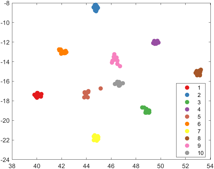
(a) our proposed coupled tensor norm regularization

(b) $\ell_{1}$-norm regularization

(c) $\ell_{2}$-norm regularization

(d) Tikhonov regularization

Figure 1: The output features learned from multinomial logistic regression with different regularizers for AR10P face dataset. Data are visualized in two dimensions using t-SNE.

From the practical implementation point of view, there exist two difficulties in optimizing the loss function with the coupled tensor norm regularization. Firstly, this coupled norm is nonconvex and nonsmooth in general. Secondly, the coupled tensor norm regularized model is nonseparable. Our main contributions are as follows.

• We propose a coupled tensor norm regularization which enables the input tensor data and the output feature matrix to lie in a low dimensional manifold. Further, we present the convexity and smoothness analysis of this regularization function.

• For multinomial logistic regression, we show the coupled tensor norm regularization is convex, differentiable, and its gradient is Lipschitz continuous. The gradient descent approach is adopted to solve the model and we analyze its global convergence.

• For deep neural networks, we show the loss function with the coupled tensor norm is nonconvex and non-differentiable. Further, we introduce an auxiliary variable to derive the quadratic penalty formulation. Then we present an alternating minimization method to overcome the nonseparability. We show this nonconvex and nonsmooth optimization problem is convergent based on the KŁ property.

• We conduct numerical experiments on a series of real datasets for both multinomial logistic regression and deep neural networks. Compared with the $\ell_{1}$-norm, $\ell_{2}$-norm, and Tikhonov regularizations, our proposed coupled norm regularization performs better in terms of testing accuracy, especially for small data problems.

1.1 Related work

Low-dimensional manifold. As discussed in [21, 22], researchers proved that the patch set of many classes of images could come from a low-dimensional manifold. Afterwards, the low-dimensional manifold model (LDMM) [19] was raised to compute the dimension of the patch set based on the differential geometry. Then the dimension was used as the regularization term for the image recovery problem. Recently, under an assumption that the concatenation of the input data and the output features should sample a collection of low-dimensional manifolds, LDMNet [34] was proposed to regularize the deep neural network and outperformed some widely-used regularizers. All above models require solving the variational subproblems to get a low-dimensional manifold. Specifically, the Euler-Lagrange equation caused by subproblem needs to be solved by using discretization and point integral method, which is complex relatively.

Tensor methods for generalization. A recent line of generalization study focuses on tensor methods. For instance, [14] advanced the understanding of the relations between the network’s architecture and its generalizability from the compression perspective. [10] proposed tensor dropout, a randomization technique that can be applied to tensor factorizations, for improving generalization. Moreover, tensor methods [6] can also be used to design efficient deep neural networks with stronger generalization. Please see [20] for a review of tensor methods in computer vision and deep learning.

Coupled tensor norm. The joint factorization of coupled matrices and tensors (hereafter coupled tensors) has shown its power in improving our understanding of the underlying structures in complex data sets such as social networks [2]. Early studies on coupled factorization methods are usually nonconvex and the ranks of the coupled tensors need to be determined beforehand. To overcome the above bottlenecks, the coupled tensor norms [25, 31, 32] were proposed for structured tensor computation, which are convex approaches for coupled tensor decomposition.

2 Preliminaries

Tensors. For an $N$-way tensor $\mathcal{X}\in\mathbb{R}^{I_{1}\times\cdots\times I_{N}}$, the mode-$n$ unfolding matrix is $X_{(n)}\in\mathbb{R}^{I_{n}\times J_{n}}$, where $J_{n}=\prod\limits_{i=1,i\neq n}^{N}I_{i}$. Further, the Tucker decomposition of $\mathcal{X}$ is

$$\mathcal{X}=\mathcal{G}\times_{1}U_{1}\times_{2}U_{2}\times_{3}\dots\times_{N}U_{N},$$

or equivalently,

$$X_{(n)}=U_{n}G_{(n)}\left(U_{N}\otimes\dots\otimes U_{n+1}\otimes U_{n-1}\dots\otimes U_{1}\right)^{\top},$$

where $U_{n}\in\mathbb{R}^{I_{n}\times R_{n}}$ for $n=1,\dots,N$ are the factor matrices (which are usually orthogonal) and $\mathcal{G}\in\mathbb{R}^{R_{1}\times\dots\times R_{N}}$ is the core tensor. The multilinear rank of $\mathcal{X}$ is defined as $(R_{1},\cdots,R_{N})$. Here, $R_{n}$ is also the rank of the mode-$n$ unfolding matrix of $\mathcal{X}$. We refer to the reviewer paper [11] for more details.

Coupled tensor norm. Suppose the $n$-the order of tensor $\mathcal{X}\in\mathbb{R}^{I_{1}\times\cdots\times I_{N}}$ shares the same feature with the rows of a matrix $A\in\mathbb{R}^{I_{n}\times J}$. The coupling of $\mathcal{X}$ and $A$ can provide more information on the features. Please see Figure 2 for an example that a third order tensor and a matrix are coupled at mode-1. The coupled low-rank decomposition of $\mathcal{X}$ and $A$ seeks for the factors $U_{i}\in\mathbb{R}^{I_{i}\times R_{i}}$ for $i=1,\dots,N$ and $V\in\mathbb{R}^{J\times R_{n}}$ such that

$$\mathcal{X}\approx\mathcal{G}\times_{1}U_{1}\times_{2}U_{2}\times_{3}\dots\times_{N}U_{N}\text{ and }A\approx U_{n}V^{\top}.$$

Note that $U_{n}$ is shared between $\mathcal{X}$ and $A$ with a coupled rank $R_{n}$. However, the above equation needs to specify the rank beforehand. To overcome this difficulty, [30] proposed the coupled tensor norm of $[\mathcal{X},A]$ based on the overlapped approach, i.e.,

$$\|\mathcal{X},A\|_{\hbox{c}}:=\|X_{(n)},A\|_{*}+\sum\limits_{i=1,i\neq n}^{N}\|X_{(i)}\|_{*},$$ (1)

which arises from convex approaches for low-rank decomposition of coupled tensor and matrix. Here, the nuclear norm function is convex but nonsmooth. More specifically, for matrix $A$ with thin SVD decomposition $A=USV^{\top}$, its subgradient is

$$\partial\|A\|_{*}=\{UV^{\top}+Z\mid U^{\top}Z=0,ZV=0,\|Z\|\leq 1\}.$$

Note that (1) does not need to specify the rank beforehand and can obtain the low-rank property automatically.

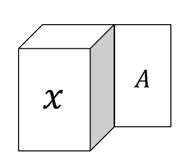
Figure 2: Illustration of the coupling between a tensor $\mathcal{X}$ and a matrix $A$ at the first mode.

Variational analysis. Let $f:\mathbb{R}^{n}\to\mathbb{R}\cup\{+\infty\}$ be an extended function. $f$ is called regular at $\bar{x}$ if the set epi($f$) is Clarke regular at $(\bar{x},f(\bar{x}))$. Here, $\hbox{epi}(f)=\{(x,r)\mid f(x)\leq r\}$ is the epigraph of $f$. Furthermore, if each $f_{i}\;(1\leq i\leq n)$ is regular at $\bar{x}$, then $f=\sum\limits_{i=1}^{n}f_{i}$ is regular at $\bar{x}$ and

$$\partial f(\bar{x})=\partial f_{1}(\bar{x})+\cdots+\partial f_{n}(\bar{x}).$$ (2)

The interested reader can refer to, e.g., [1], for more properties of Clarke regular and regularity.

3 Method

Consider the multi-classification with $n$ samples and $c$ disjoint classes. Let $S=\{(\mathcal{X}_{i},y_{i})\}_{i=1}^{n}$ denote independent and identically distributed training dataset, where $\mathcal{X}_{i}\in\mathbb{R}^{I_{1}\times\dots\times I_{N}}$ is the input data information and $y_{i}\in\mathbb{R}^{c}$ is the corresponding label. Denote $m=\prod_{i=1}^{N}I_{i}$ as the number of input features. Here, $y_{i}=(y_{i}^{(1)},y_{i}^{(2)},\cdots,y_{i}^{(c)})^{\top}$ is the one-hot vector with $y_{i}^{(k)}=1$ if $\mathcal{X}_{i}$ belongs to the $k$-th class and $y_{i}^{(k^{\prime})}=0$ otherwise. For convenience, let $\mathcal{X}\in\mathbb{R}^{n\times I_{1}\times\dots\times I_{N}}$ and $Y\in\mathbb{R}^{n\times c}$ denote the concatenation of $\mathcal{X}_{i}$ and $y_{i}$ at the first mode, respectively. Also, denote $f_{\theta}(\mathcal{X}_{i})\in\mathbb{R}^{c}$ as the output feature of $\mathcal{X}_{i}$. The loss function of the classification model is

$$\min\limits_{\theta}\;L(\theta),\ \text{where }L(\theta)=\frac{1}{n}\sum_{i=1}^{n}l(f_{\theta}(\mathcal{X}_{i}),y_{i}),$$ (3)

where $l(\cdot)$ is the loss function, such as the cross entropy loss.

Denote $f_{\theta}(\mathcal{X})\in\mathbb{R}^{n\times c}$ as the concatenation of $f_{\theta}(\mathcal{X}_{i})$ at the first mode. As discussed in [34], the concatenation $\mathcal{X}$ and $f_{\theta}(\mathcal{X})$ should sample a collection of low dimensional manifolds to reduce the risk of overfitting. This idea is due to the Gaussian mixture model: the tuples $\{(\mathcal{X}_{i},f_{\theta}(\mathcal{X}_{i}))\}_{i=1}^{n}$ are generated by a mixture of low dimensional manifolds. Namely, suppose the coupled decomposition is

$$\mathcal{X}\approx\mathcal{G}\times_{1}U_{1}\times_{2}U_{2}\times_{3}\dots\times_{N+1}U_{N+1}\text{ and }f_{\theta}(\mathcal{X})\approx U_{1}V^{\top},$$

where $U_{1}\in\mathbb{R}^{n\times R_{1}}$, $U_{i}\in\mathbb{R}^{I_{i-1}\times R_{i}}$ for $i=2,\dots,N+1$, and $V\in\mathbb{R}^{c\times R_{1}}$. Then the joint rank $R_{1}$ in the above formulation should be small. However, we do not know the joint rank in advance. Hence, the coupled tensor norm based on the overlapped approach in (1) is adopted to characterize low-rankness, and we have

$$\|\mathcal{X},f_{\theta}(\mathcal{X})\|_{c}=\|X_{(1)},f_{\theta}(\mathcal{X})\|_{*}+\sum\limits_{i=2}^{N+1}\|X_{(i)}\|_{*}.$$ (4)

Note that only the first term depends on $\theta$. By ignoring the terms independent of $\theta$, we propose the following regularization function,

$$R(\theta)=\|X_{(1)},f_{\theta}(\mathcal{X})\|_{*}.$$ (5)

Consequently, the classification model (3) can be formulated as the following general minimization problem,

$$\min\limits_{\theta}\;L(\theta)+\lambda R(\theta),$$ (6)

where $\lambda>0$ is the parameter.

In the following theorem, we show the properties of the matrix concatenation function.

Theorem 3.1.

Let $X\in\mathbb{R}^{n\times m}$ and $\xi\in\mathbb{R}^{n\times c}$. Then the matrix row concatenation function $g(\xi)=\|X,\xi\|_{*}$ is not a norm. Further, it is a convex but nonsmooth function of $\xi$, and the subgradient of $g(\xi)$ is

$$\partial g(\xi)=\{UV_{2}^{\top}+Z_{2}\,|\,U^{\top}Z=0,ZV=0,\|Z\|_{2}\leq 1\},$$

where $U\Sigma V^{\top}$ is the thin SVD of $[\mathcal{X},\xi]$, $r$ is the rank of $[\mathcal{X},\xi]$, $U\in\mathbb{R}^{n\times r}$, $\Sigma\in\mathbb{R}^{r\times r}$, $V\in\mathbb{R}^{(m+c)\times r}$, $V_{2}\in\mathbb{R}^{c\times r}$ is the last $c$ rows of $V$, and $Z_{2}\in\mathbb{R}^{n\times c}$ is the last $c$ columns of $Z\in\mathbb{R}^{n\times(m+c)}$.

Proof.

Note that when $\xi$ is equal to zero, $g(\xi)$ may not equal zero. Hence, $g(\xi)$ is not a norm.

Further, by rewriting the concatenation of $X$ and $\xi$ as a linear function of $\xi$,

$$[X,\xi]=\xi A+[X,O],$$ (7)

where $A=[O,I]$, $O$ is the $c$-by-$m$ zero matrix, and $I$ is the $c$-by-$c$ identity matrix, we have that $g(\xi)$ is the composition of convex and linear functions. Hence, $g(\xi)$ is convex consequently. By the thin SVD decomposition $USV^{\top}$ of matrix $[X,\xi]$, the subdifferential of the nuclear norm at $[X,\xi]$ is

$$\partial\|X,\xi\|_{*}=\{UV^{\top}+Z\mid U^{\top}Z=0,ZV=0,\|Z\|\leq 1\}.$$

Through the chain rule and equation (7), we have

$$\partial g(\xi)=\frac{\partial g(\xi)}{\partial[X,\xi]}\cdot\frac{\partial[X,\xi]}{\partial\xi} =(UV^{\top}+Z)A^{\top}$$

$$=UV^{\top}_{2}+Z_{2},$$ (8)

where $V_{2}$ is the last $c$ rows of $V$ and $Z_{2}$ is the last $c$ columns of $Z$. This completes the proof. ∎

Based on Theorem 3.1, we can analyze the properties of our proposed regularizer, which is the composition of matrix nuclear norm, matrix concatenation, and classification model.

Theorem 3.2.

Let $R(\theta)$ be the regularizer defined by (5). Then,

• if $f_{\theta}(\mathcal{X})$ is a linear function with respect to $\theta$, then $R(\theta)$ is convex. Further, if $f_{\theta}(\mathcal{X})=X_{(1)}\theta$ or $f_{\theta}(\mathcal{X})=X_{(1)}\theta^{\top}$, then $R(\theta)$ is also smooth;

• if $f_{\theta}(\mathcal{X})$ is a general nonconvex and nonsmooth function with respect to $\theta$, then $R(\theta)$ is nonconvex and nonsmooth.

Proof.

If $\xi=f_{\theta}(\mathcal{X})$ in Theorem 3.1 is a linear function with respect to $\theta$, then $R(\theta)$ is the composition of convex and linear functions, and is convex consequently. On the other hand, when $f_{\theta}(\mathcal{X})$ is a general nonconvex and nonsmooth function with respect to $\theta$, $R(\theta)$ is nonconvex and nonsmooth. Furthermore, based on SVD decomposition $USV^{\top}$ of matrix $[X_{(1)},f_{\theta}(\mathcal{X})]$, we have

$$X_{(1)}=USV_{1}^{\top},\;\;f_{\theta}(\mathcal{X})=USV_{2}^{\top},$$

where $V_{1},V_{2}$ are the front $m$ rows and the last $c$ rows of $V$, respectively. From (3) in the proof of Theorem 3.1, we have if $f_{\theta}(\mathcal{X})=X_{(1)}\theta$,

$$\nabla R(\theta)=V_{1}SU^{\top}(UV_{2}^{\top}+Z_{2})=V_{1}SV_{2}^{\top},$$

and if $f_{\theta}(\mathcal{X})=X_{(1)}\theta^{\top}$,

$$\nabla R(\theta)=(UV_{2}^{\top}+Z_{2})^{\top}USV_{1}^{\top}=V_{2}SV_{1}^{\top}.$$ (9)

Hence, $R(\theta)$ is smooth in these two cases. The proof is completed. ∎

3.1 Multinomial logistic regression

Multinomial logistic regression (MLR) is a classical learning method for classification. Let $x_{i}\in\mathbb{R}^{m}$ be the vectorization of the input tensor $\mathcal{X}_{i}$ and $X\in\mathbb{R}^{n\times m}$ denote all input features of $n$ training samples which is the unfolding matrix of $\mathcal{X}$ at the first mode. The probability that $x_{i}$ belongs to the $k$-th class is modeled by the softmax function as follows,

$$P(y_{i}^{(k)}=1\mid x_{i},W):=\frac{\exp(w_{k}^{\top}x_{i})}{\sum\limits_{j=1}^{c}\exp(w_{j}^{\top}x_{i})},$$

where $w_{j}\in\mathbb{R}^{m}$ is the $j$-th weight vector, $W:=(w_{1},w_{2},\cdots\\ ,w_{c})^{\top}\in\mathbb{R}^{c\times m}$ is the weight matrix to be estimated from the training set. Furthermore, MLR adopts the maximum likelihood estimation to estimate the weight matrix $W$. The corresponding loss function is

$$L(W)=-\frac{1}{n}\sum\limits_{i=1}^{n}\big{(}\sum\limits_{j=1}^{c}y_{i}^{(j)}w_{j}^{\top}x_{i}-\log\sum\limits_{j=1}^{c}\exp(w_{j}^{\top}x_{i})\big{)},$$

which is corresponding to equation (3) with $\theta=\{W\}$, $f_{\theta}(X)$ being a linear formulation $XW^{\top}$, and $l(\cdot)$ being the cross entropy loss.

The above MLR model may fail to generalize well on the testing dataset when the number of data $n$ is much smaller than the number of data features $m$ [33]. To improve the generalization, the proposed model (6) can be written as

$$\min\limits_{W\in\mathbb{R}^{c\times m}}\;G(W):=L(W)+\lambda\|X,XW^{\top}\|_{*}.$$ (10)

It is well known that the nuclear norm function itself is nonsmooth. However, the coupled nuclear norm proposed in this context is differentiable with respect to $W$. More details are presented in the following lemma.

Lemma 3.1.

Let regularization term $R(W)=\|X,XW^{\top}\|_{*}$ in model (10), and $USV^{\top}$ be its SVD decomposition. Divide $V$ as $[V_{1},V_{2}]$ with $V_{1}\in\mathbb{R}^{n\times m}$ and $V_{2}\in\mathbb{R}^{n\times c}$. Then we have

• $R(W)$ is differentiable with respect to $W$ and its gradient is $V_{2}SV_{1}^{\top}$;

• $\nabla R(W)$ is Lipschitz continuous if all singular values of matrix $XW^{\top}$ are nonzeros.

Proof.

The regularization $\|X,XW^{\top}\|_{*}$ in model (10) is a special case of (5). Hence, we can get the gradient of $R(W)$ from (9), i.e.,

$$\nabla R(W)=V_{2}SV_{1}^{\top}.$$

Furthermore, for any matrices $W,\hat{W}\in\mathbb{R}^{c\times m}$, we have

$$\|\nabla R(W)-\nabla R(\hat{W})\|_{F}=\|V_{2}SV_{1}^{\top}-\hat{V}_{2}^{\top}\hat{S}\hat{V}_{1}^{\top}\|_{F}=\|CB\|_{F},$$

where $B=\begin{pmatrix}USV_{1}^{\top}\\ -\hat{U}\hat{S}\hat{V}_{1}^{\top}\end{pmatrix}$, $C=(V_{2}U^{\top},\hat{V}_{2}^{\top}\hat{U}^{\top})$. Owing to the fact that the largest singular value of $C$ satisfies $\sigma_{\max}(C)\leq 1$, we have

$$\|\nabla R(W)-\nabla R(\hat{W})\|_{F}\leq\|B\|_{F}.$$ (11)

By denoting $E=\begin{pmatrix}V_{2}SU^{\top},\hat{V}_{2}\hat{S}\hat{U}^{\top}\end{pmatrix}=\begin{pmatrix}WX^{\top},\hat{W}X^{\top}\end{pmatrix}$, we have

$$\|X^{\top}XW^{\top}-X^{\top}X\hat{W}^{\top}\|_{F}$$

$$= \|V_{2}S^{2}V_{1}^{\top}-\hat{V}_{2}\hat{S}^{2}\hat{V}_{1}^{\top}\|_{F}$$

$$= \|V_{2}SU^{\top}USV_{1}^{\top}-\hat{V}_{2}\hat{S}\hat{U}^{\top}\hat{U}\hat{S}V_{1}^{\top}\|_{F}$$

$$= \|EB\|_{F}$$

$$\geq \sigma_{\min}(E)\|B\|_{F},$$ (12)

where $\sigma_{\min}(E)$ denotes the smallest singular value of $E$. Under the assumption that all singular values of $XW^{\top}$ is nonzero for all $W$ and the fact that $E$ is the concatenation of $WX^{\top}$ and $\hat{W}X^{\top}$, we have $\sigma_{\min}(E)>0$. Combining (11) and (3.1), we have

$$\|\nabla R(W)-\nabla R(\hat{W})\|_{F}$$

$$\leq \|B\|_{F}$$

$$\leq \frac{1}{\sigma_{\min}(E)}\|X^{\top}XW^{\top}-X^{\top}X\hat{W}^{\top}\|_{F}$$

$$\leq \frac{\lambda_{\max}(X^{\top}X)}{\sigma_{\min}(E)}\|W-\hat{W}\|_{F}.$$

Hence, $\nabla R(W)$ is Lipschitz continuous and this completes the proof. ∎

The intrinsic convexity and differentiability of model (10) inspire us to utilize the classical gradient descent algorithm with linesearch to solve it.

Algorithm description. The iterative process for updating $W^{k+1}$ is based on following procedure,

$$W^{k+1}=W^{k}+\alpha_{k}\nabla G(W^{k}).$$ (13)

Here, $\alpha_{k}$ is obtained by a linesearch algorithm with guaranteed sufficient decrease which was introduced in [17].

For a given threshold $\varepsilon\geq 0$, the termination criterion is $\|\nabla G(W)\|_{2}\leq\varepsilon$. The convergence analysis is illuminated in the next theorem.

Theorem 3.3.

Suppose all singular values of output matrix $XW^{\top}$ are nonzeros. For the convex differential minimization problem (10), each accumulation point of the iterative sequence $\{W^{k}\}_{k=0}^{\infty}$ generated by procedure (13) is a global minimizer.

Proof.

The iterative procedure (13) is a gradient descent method with the stepsize $\alpha_{k}$ satisfying the Wolfe-Powell rules, and $\nabla G(W)$ in model 10 is Lipschitz continuous based on Lemma 3.1. Hence, as introduced in [27, Theorem 2.5.7], for the sequence $\{W^{k}\}_{k=0}^{\infty}$ generated by the gradient descent method with Wolfe linesearch, either $\|\nabla G\\ (W^{k})\|_{2}=0$ for some $k$ or $\|\nabla G(W^{k})\|_{2}\to 0$. It means that each accumulation point of the iterative sequence $\{W^{k}\}_{k=0}^{\infty}$ is a stationary point. Furthermore, the stationary point is also a global minimizer owing to the convexity of model (10). This completes the proof. ∎

3.2 Deep neural networks (DNN)

Let $\theta$ be the collection of network weights and bias. For every data $\mathcal{X}_{i}$, the classical DNN learns a feature $f_{\theta}(\mathcal{X}_{i})\in\mathbb{R}^{c}$ by minimizing the empirical loss function on the training data as defined by (3). To reduce the risk of overfitting of DNN [29], we apply the coupled tensor norm regularization (5) into the loss function and propose the regularized DNN model as

$$\min_{\theta}~{}L(\theta)+\lambda\|X_{(1)},f_{\theta}(\mathcal{X})\|_{*},$$ (14)

where $f_{\theta}(\mathcal{X})\in\mathbb{R}^{n\times c}$ is highly nonlinear and nonsmooth. Therefore, from Theorem 3.2, the regularization term in model (14) is nonconvex, nonsmooth, and nonseparable.

A basic condition for solving DNN by the stochastic gradient descent (SGD) method is that the objective function is separable. To circumvent the nonseparability of (14), we introduce an auxiliary variable $\xi$ into (14) as follows:

$$\min_{\theta,\xi}~{}L(\theta)+\lambda\|X_{(1)},\xi\|_{*},\text{ s.t. }f_{\theta}(\mathcal{X})=\xi.$$

Then we penalize the constraint into the loss function using the quadratic penalty method and get the following unconstrained model:

$$\min_{\theta,\xi}~{}\mathcal{L}(\theta,\xi):=L(\theta)+\lambda\|X_{(1)},\xi\|_{*}+\frac{\mu}{2}\|f_{\theta}(\mathcal{X})-\xi\|^{2}_{F},$$ (15)

where $\mu>0$ is the penalty parameter. Problem (15) is solved by alternating the directions of $\theta$ and $\xi$. Specifically, given $(\theta^{k},\xi^{k})$, we implement the following sub-steps:

• Update $\theta^{k+1}$ with the fixed $\xi^{k}$:

  $$\min_{\theta}~{}L(\theta)+\frac{\mu}{2}\|f_{\theta}(\mathcal{X})-\xi^{k}\|^{2}_{F}.$$ (16)

• Update $\xi^{k+1}$ with the fixed $\theta^{k+1}$:

  $$\min_{\xi}~{}\lambda\|X_{(1)},\xi\|_{*}+\frac{\mu}{2}\|f_{\theta^{k+1}}(\mathcal{X})-\xi\|^{2}_{F}.$$ (17)

The $\theta$-subproblem (16) is separable with respective to the samples $\mathcal{X}_{i}$ and can be solved by SGD. The $\xi$-subproblem (17) is strongly convex but nonsmooth by Theorem 3.1. Based on the above analysis, we describe our algorithm framework for solving (15) in Algorithm 1.

Algorithm 1 The alternating minimization method for (15)

0:  Training data $\{(\mathcal{X}_{i},y_{i})\}_{i=1}^{n}$, hyperparameters $\lambda$ and $\mu$, and a neural network with initial weight $\theta^{0}$.

0:  Trained network weights $\theta^{*}$. Let $k=0$. $\xi^{0}\in\mathbb{R}^{n\times c}$ is initialized as zero.

  while not converge do

     1. Update $\theta^{k+1}$in(16): solve the nonconvex problem by SGD.

     2. Update $\xi^{k+1}$ in (17): solve the convex problem by the subgradient method.

     3. $k\leftarrow k+1$.

  end while$\theta^{*}=\theta^{k}$.

Next, we show the global convergence of Algorithm 1 based on the KŁ property and regularity under the following mild assumption.

Assumption 3.1.

Assume the following conditions hold.

• The loss function $\mathcal{L}(\theta,\xi)$ defined by (15) is regular and satisfies the KŁ property.

• The subgradient of $f_{\theta}(\mathcal{X})$ is upper bounded, i.e., there exists a positive constant $\rho$ such that for all $g_{f}\in\partial f_{\theta}(\mathcal{X})$, we have $\|g_{f}\|\leq\rho.$

Theorem 3.4.

Suppose Assumption 3.1 holds. Let the sequence $\{(\theta^{k},\xi^{k})\}_{k\geq 0}$ be generated by Algorithm 1. Then $\{\xi^{k}\}_{k\geq 0}$ has finite length and converges to a point $\xi^{*}$ globally. Moreover, let $\theta^{*}$ be any limit point of the sequence $\{\theta^{k}\}_{k\geq 0}$, then $(\theta^{*},\xi^{*})$ is a critical point of $\mathcal{L}$.

Proof.

We firstly show the sequence $\{(\theta^{k},\xi^{k})\}_{k\geq 0}$ generated by Algorithm 1 satisfies the four conditions for the bounded approximate gradient-like descent sequence in [8, Definition 2].

For the $\theta$ subproblem in (16) and the $\xi$ subproblem in (17), we have respectively,

$$\mathcal{L}(\theta^{k+1},\xi^{k})\leq\mathcal{L}(\theta^{k},\xi^{k}),$$ (18)

$$0\in\partial_{\xi}\mathcal{L}(\theta^{k+1},\xi^{k}).$$ (19)

Since $\mathcal{L}(\theta,\xi)$ is strongly convex with respect to $\xi$, we can get that for all $g^{k+1}_{\xi}\in\partial_{\xi}\mathcal{L}(\theta^{k+1},\xi^{k+1})$, it holds that

$$\mathcal{L}(\theta^{k+1},\xi^{k+1})+\langle g^{k+1}_{\xi},\xi^{k}-\xi^{k+1}\rangle +\frac{\mu}{2}\|\xi^{k}-\xi^{k+1}\|_{2}^{2}$$

$$\leq\mathcal{L}(\theta^{k+1},\xi^{k}).$$

Furthermore, adding (18) to the above inequality and combining it with (19) yield

$$\frac{\mu}{2}\|\xi^{k}-\xi^{k+1}\|_{2}^{2}\leq\mathcal{L}(\theta^{k},\xi^{k})-\mathcal{L}(\theta^{k+1},\xi^{k+1}).$$ (20)

It is clear that condition C1 in [8, Definition 2] holds.

Secondly, from (19), (2), and Assumption 3.1, we can obtain

$$0 \in\partial_{\theta}\mathcal{L}(\theta^{k+1},\xi^{k})$$

$$=\partial L(\theta^{k+1})+\mu\partial f_{\theta^{k+1}}(\mathcal{X})^{\top}(f_{\theta^{k+1}}(\mathcal{X})-\xi^{k})$$

$$=\partial L(\theta^{k+1})+\mu\partial f_{\theta^{k+1}}(\mathcal{X})^{\top}(f_{\theta^{k+1}}(\mathcal{X})-\xi^{k+1})$$

$$\quad+\mu\partial f_{\theta^{k+1}}(\mathcal{X})^{\top}(\xi^{k+1}-\xi^{k}).$$

Combing it with (19), we get

$$W^{k+1}=\begin{pmatrix}\mu g_{f}^{\top}(\xi^{k}-\xi^{k+1})\\ 0\end{pmatrix}\in\partial\mathcal{L}(\theta^{k+1},\xi^{k+1}),$$

where $g_{f}\in\partial f_{\theta^{k+1}}(\mathcal{X})$. Then, with triangle inequality and Assumption 3.1,

$$\|W^{k+1}\|\leq\mu\|g_{f}\|\|\xi^{k}-\xi^{k+1}\|\leq\mu\rho\|\xi^{k}-\xi^{k+1}\|.$$ (21)

At last, if $(\bar{\theta},\bar{\xi})$ is a limit point of some sub-sequence $\{(\theta^{k},\xi^{k})\}_{k\in\mathcal{K}\subseteq\mathbb{K}}$, based on the continuity of objective function $L(\theta,\xi)$, we can obtain

$$\limsup_{k\in\mathcal{K}\subseteq\mathbb{K}}\mathcal{L}(\theta^{k},\xi^{k})\leq\mathcal{L}(\bar{\theta},\bar{\xi}).$$ (22)

Moreover, the condition C4 in [8, Definition 2] holds clearly when the subproblems (16) and (17) are solved exactly. Combining (20), (21), and (22), we have that the sequence $\{(\theta^{k},\xi^{k})\}_{k\geq 0}$ generated by Algorithm 1 is an approximate gradient-like descent sequence in [8].

Furthermore, let $u:=(\theta,\xi)$ for convenience. The function $\mathcal{L}(u)$ is proper, lower semicontinuous, which has the KŁ property directly. Hence, we can get the convergence with the KŁ property [5] and the approximate gradient-like descent sequence by Theorem 1 in [8]. ∎

Remark 3.1.

Actually, the subproblems (16) and (17) can also be solved inexactly. We can find approximate solution for (16) and (17) until the following criteria satisfied,

$$\frac{\mu}{2}\|\xi^{k}-\xi^{k+1}\|_{2}^{2}-(e_{1}^{k})^{2} \leq\mathcal{L}(\theta^{k},\xi^{k})-\mathcal{L}(\theta^{k+1},\xi^{k+1}),$$

$$\|W^{k+1}\|-e_{2}^{k} \leq\mu\rho\|\xi^{k}-\xi^{k+1}\|,$$

where $\{e_{1}^{k}\}_{k\geq 0}$ and $\{e_{2}^{k}\}_{k\geq 0}$ are required to be summable. Together with (22), the sequence $\{(\theta^{k},\xi^{k})\}_{k\geq 0}$ is also an approximate gradient-like descend sequence defined in [8].

Remark 3.2.

By [36], the assumption that $\mathcal{L}$ is regular near $(\theta^{*},\xi^{*})$ can be satisfied for some deep neural networks with the ReLU activation function.

4 Numerical Experiments

In this section, we verify the efficiency of our proposed coupled tensor norm regularization for both MLR and DNN on nine real datasets listed in Table 1. We first test the performance of MLR on three face image datasets (ORL, Yale, AR10P) and three biological datasets (lung, TOX-171, lymphoma) downloaded online . Then we test the performance of DNN on Fashion-MNIST, CIFAR-10, and an MRI dataset (Brain Tumor) .

Table 1: Details of all datasets. $n$ and $n^{\prime}$ are the number of training and testing samples, respectively. $m$ denotes the number of features and $c$ is the number of classes.

Dataset	$n$	$n^{\prime}$	$m$	$c$
ORL	280	120	1024	40
Yale	100	65	1024	15
AR10p	90	40	2400	10
Lung	153	50	3312	5
TOX-171	100	71	5748	4
Lymphoma	56	40	4026	9
Fashion-MNIST	60000	10000	784	10
CIFAR-10	60000	10000	3072	10
Brain Tumor	2870	394	50176	4

4.1 Multinomial logistic regression

Table 2: Numerical results of multinomial logistic regression for three face datasets.

	ORL			Yale			AR10P
Model	Training	Testing	$\lambda$	Training	Testing	$\lambda$	Training	Testing	$\lambda$
MLR	95.71%	90.83%	0	90.00%	75.38%	0	85.56%	90.00%	0
MLR-$\ell_{1}$	96.07%	93.33%	$10^{-4}$	89.00%	75.38%	$10^{-6}$	85.56%	92.50%	$10^{-3}$
MLR-$\ell_{2}$	96.07%	93.33%	$10^{-6}$	89.00%	75.38%	$10^{-6}$	85.56%	95.00%	$10^{-4}$
MLR-Tik	96.42%	93.33%	1	90.00%	78.46%	0.1	85.56%	97.50 %	$10^{-2}$
MLR-ours	96.07%	95.00%	$10^{-4}$	92.00%	81.54%	$10^{-5}$	85.56%	100%	$10^{-5}$

Table 3: Numerical results of multinomial logistic regression for three biological datasets.

	Lung			TOX-171			Lymphoma
Model	Training	Testing	$\lambda$	Training	Testing	$\lambda$	Training	Testing	$\lambda$
MLR	95.43%	86.00%	0	75.00%	57.75%	0	98.21%	85.00%	0
MLR-$\ell_{1}$	93.46%	92.00%	$10^{-2}$	66.00%	63.38%	$10^{-2}$	98.21%	90.00%	$10^{-2}$
MLR-$\ell_{2}$	94.12%	94.00%	$10^{-2}$	66.00%	61.97%	$10^{-4}$	98.21%	87.50%	$10^{-3}$
MLR-Tik	96.08%	96.00%	$10^{-1}$	72.00%	67.61%	1	98.21%	95.00%	1
MLR-ours	96.08%	96.00%	$10^{-2}$	71.00%	69.01%	$10^{-2}$	98.21%	95.00%	1

Table 4: Comparisons of difference $\lambda$ between ours and Tikhonov regularization for MLR on Lymphoma dataset.

$\lambda$	$1$	$10^{-1}$	$10^{-2}$	$10^{-3}$	$10^{-4}$	$10^{-5}$	$10^{-6}$
MLR-Tik	95.00%	82.50%	67.50%	42.50%	42.50%	45.00%	45.00%
MLR-ours	95.00%	92.50%	87.50%	82.50%	82.50%	82.50%	82.50%

In this subsection, we compare the coupled tensor norm regularization model (10) with the $\ell^{1}$-norm [23], $\ell^{2}$-norm [18], Tikhonov regularization [4] models. For all regularized models, we traverse $\lambda$ from $\{10^{-6},10^{-5},10^{-4},10^{-3},\\ 10^{-2},10^{-1},1\}$ and report the results corresponding to $\lambda$ with the highest classification accuracy. The gradient or subgradient descent algorithm is adopted to solve the models. The corresponding stopping criteria is set as

$$\|W^{k+1}-W^{k}\|_{F}\leq 10^{-4}\;\;\hbox{or}\;\;\|\nabla G(W^{k})\|_{2}\leq 10^{-4},$$

and the maximum number of iterations is 2000. Moreover, we initialize $W^{0}=0$.

The training accuracy, testing accuracy, and the choices of the optimal parameters on the face and biological datasets are elaborated in Tables 2 and 3, respectively. For all six datasets, our regularization guarantees the highest testing accuracy and lowest generalization error. We further compare the coupled tensor norm and Tikhonov regularizations for all $\lambda$ in Table 4, which shows that our regularization is more robust.

4.2 Deep neural networks

We continue to compare the performance of DNN with the coupled norm regularization with the $\ell_{1}$ norm [15] and Tikhonov regularization [13]. The network structures we tested VGG-16 [35]. Also, we verify the efficiency of our proposed method by setting the number of training samples from small to large.

For all methods, the hyperparameters $\lambda$ and $\mu$ are optimized from $\{10^{-i},5\cdot 10^{-i}\}_{i=1}^{6}$ and we only report the best performance. The implementation details and the choices of hyperparameters are given in the appendix. For Fashion-MNIST, we show the performance of different regularizers with varying training sizes from 1000 to 60000. The detailed result is shown in Table 5.

Table 5: The testing accuracy of different regularizers for VGG-16 on Fashion-MNIST.

Model	VGG-16 on Fashion-MNIST
Training per class	DNN	DNN-$\ell_{1}$	DNN-Tik	DNN-ours
100	80.95%	82.40%	82.16%	83.38%
400	86.95%	87.78%	87.13%	88.15%
700	88.60%	90.03%	89.66%	90.73%
1000	90.67%	90.85%	90.76%	91.28%
3000	92.13%	92.70%	92.62%	92.93%
6000	93.88%	94.29%	94.30%	94.73%

At last, we present the results for CIFAR-10 and Brain Tumor in Tables 6 and 7, respectively. The numerical experiments show that the generalization ability of our coupled norm regularizer is better than the baselines.

Table 6: The testing accuracy of different regularizers for VGG-16 on CIFAR-10.

Model	VGG-16 on CIFAR-10
Training per class	DNN	DNN-$\ell_{1}$	DNN-Tik	DNN-ours
100	48.57%	49.10%	48.98%	50.26%
400	72.90%	73.29%	73.32%	74.15%
700	78.97%	79.14%	79.31%	80.29%

Table 7: Numerical results of different regularizations for VGG-16 on the MRI dataset Brain Tumor.

	VGG-16 on Brain Tumor
Model	Training	Testing	$\lambda~{}(\mu)$
DNN	99.50%	75.48%	0
DNN-$\ell_{1}$	99.97%	76.40%	$10^{-3}$
DNN-Tik	99.83%	76.67%	$10^{-3}$
DNN-ours	99.97%	77.41%	$5\cdot 10^{-4}$ ($10^{-4}$)

5 Conclusions

In this paper, we proposed a coupled tensor norm approach to obtain better generalization for classification models. Theoretically, for MLR, we showed this regularization is convex, differentiable, and gradient Lipschitz continuous and proved the global convergence of the gradient descent method. For DNN, we showed the regularization is nonconvex and nonsmooth, and established the global convergence of the alternating minimization method. At last, we verified the efficiency of our regularization compared with the $\ell_{1}$, $\ell_{2}$, and Tikhonov regularizations.

6 Appendix

Details of numerical implementation for DNN: Unless otherwise stated, all experiments use SGD with momentum fixed at 0.9 and mini-batch size fixed as 128. The networks are trained with a fixed learning rate $r_{0}=0.01$ on the first 50 epochs, and then $r_{0}/10$ for another 50 epochs. At step 1 of Algorithm 1, $\theta$ is updated once every $M=2$ epochs of SGD. And at step 2, the step size is set to $1/k$. The stopping criterion is $\|grad_{\xi}\|_{F}<tol$, where $grad_{\xi}$ is the subgradient of (17). Further, we set $tol=10^{-2}$ and the maximum number of iterations as 50.

Table 8: Hyperparameters of DNN for Fashion-MNIST dataset.

Model	VGG-16
Training per class	DNN-$\ell_{1}$	DNN-Tik	DNN-ours
	$\lambda$	$\lambda$	$\lambda$	$\mu$
100	$10^{-5}$	$10^{-5}$	$5\cdot 10^{-4}$	$5\cdot 10^{-3}$
400	$10^{-5}$	$10^{-5}$	$5\cdot 10^{-4}$	$10^{-3}$
700	$10^{-5}$	$10^{-5}$	$5\cdot 10^{-4}$	$5\cdot 10^{-4}$
1000	$10^{-4}$	$10^{-5}$	$5\cdot 10^{-4}$	$5\cdot 10^{-4}$
3000	$10^{-4}$	$10^{-5}$	$5\cdot 10^{-4}$	$5\cdot 10^{-4}$
6000	$10^{-4}$	$10^{-5}$	$5\cdot 10^{-4}$	$5\cdot 10^{-4}$

Table 9: Hyperparameters used in CIFAR-10 dataset.

Model	VGG-16
Training per class	DNN	DNN-$\ell_{1}$	DNN-Tik	DNN-ours
	$\lambda$	$\lambda$	$\lambda$	$\lambda$	$\mu$
100	0	$10^{-4}$	$10^{-5}$	$5\cdot 10^{-5}$	$5\cdot 10^{-2}$
400	0	$10^{-4}$	$10^{-3}$	$5\cdot 10^{-4}$	$5\cdot 10^{-2}$
700	0	$10^{-3}$	$10^{-5}$	$5\cdot 10^{-4}$	$5\cdot 10^{-2}$

References

- [1] R.T. Rockafellar, R.J-B Wets, Variational analysis, Springer Science & Business Media, 2009.
- [2] E. Acar, T.G. Kolda, D.M. Dunlavy, All-at-once optimization for coupled matrix and tensor factorizations, in: MLG’11: Proceedings of Mining and Learning with Graphs, 2011.
- [3] S. Arora, R. Ge, B. Neyshabur, Y. Zhang, Stronger generalization bounds for deep nets via a compression approach, in: International Conference on Machine Learning, PMLR, 2018, pp. 254-263.
- [4] C.M. Bishop, Training with noise is equivalent to Tikhonov regularization, Neural comput. 7 (1) (1995) 108–116.
- [5] J. Bolte, A. Daniilidis, A. Lewis, The Łojasiewicz inequality for nonsmooth subanalytic functions with applications to subgradient dynamical systems, SIAM J. Optim. 17 (4) (2007) 1205–1223.
- [6] N. Cohen, A. Shashua, Convolutional rectifier networks as generalized tensor decompositions, in: International Conference on Machine Learning, PMLR, 2016, pp. 955–963.
- [7] C. Cortes, M. Mohri, A. Rostamizadeh, L2 regularization for learning kernels, in: Proceedings of the 25th Conference on Uncertainty in Artificial Intelligence, 2009, pp. 109–116.
- [8] E. Gur, S. Sabach, S. Shtern, Convergent nested alternating minimization algorithms for nonconvex optimization problems, Math. Oper. Res. (2022).
- [9] S. Ioffe, C. Szegedy, Batch normalization: Accelerating deep network training by reducing internal covariate shift, in: International Conference on Machine Learning, PMLR, 2015, pp. 448–456.
- [10] A. Kolbeinsson, J. Kossaifi, Y. Panagakis, A. Bulat, A. Anandkumar, I. Tzoulaki, P. M. Matthews, Tensor dropout for robust learning, IEEE J. Sel. Topics Signal Process. 15 (3) (2021) 630–640.
- [11] T.G. Kolda, B.W. Bader, Tensor decompositions and applications, SIAM Rev. 51 (3) (2009) 455–500.
- [12] A. Krizhevsky, I. Sutskever, G. E. Hinton, Imagenet classification with deep convolutional neural networks, in: Advances in Neural Information Processing Systems, 2012, pp. 1097-1105.
- [13] A. Krogh, J. Hertz, A simple weight decay can improve generalization, in: Advances Neural Information Processing Systems, 1991, pp. 950-957.
- [14] J. Li, Y. Sun, J. Su, T. Suzuki, F. Huang, Understanding generalization in deep learning via tensor methods, in: The 23rd International Conference on Artificial Intelligence and Statistics, PMLR, 2020, pp. 504–515.
- [15] R. Ma, J. Miao, L. Niu, P. Zhang, Transformed regularization for learning sparse deep neural networks, Neural Netw. 119 (2019) 286–298.
- [16] S.-H. Lyu, L. Wang, Z.-H. Zhou, Improving generalization of deep neural networks by leveraging margin distribution, Neural Netw. 151 (2022) 48–60.
- [17] J.J. Moré, D.J. Thuente, Line search algorithms with guaranteed sufficient decrease, ACM Trans Math Softw. 20 (3) (1994) 286–307.
- [18] E. Ndiaye, O. Fercoq, A. Gramfort, J. Salmon, Gap safe screening rules for sparse multi-task and multi-class models, in: Advances in Neural Information Processing Systems, 2015, pp. 811-819 .
- [19] S. Osher, Z. Shi, W. Zhu, Low dimensional manifold model for image processing, SIAM J Imaging Sci. 10 (4) (2017) 1669–1690.
- [20] Y. Panagakis, J. Kossaifi, G.G. Chrysos, J. Oldfield, M.A. Nicolaou, A. Anandkumar, S. Zafeiriou, Tensor methods in computer vision and deep learning, Proc. IEEE 109 (5) (2021) 863-890.
- [21] G. Peyré, Image processing with nonlocal spectral bases, Multiscale Model. Simul. 7 (2) (2008) pp. 703–730.
- [22] G. Peyré, Manifold models for signals and images, Comput Vis Image Underst. 113 (2) (2009) 249–260.
- [23] M. Schmidt, G. Fung, R. Rosales, Fast optimization methods for regularization: A comparative study and two new approaches, in: European Conference on Machine Learning, Springer, 2007, pp. 286–297.
- [24] B. Shekar, G. Dagnew, L1-regulated feature selection and classification of microarray cancer data using deep learning, in: Proceedings of 3rd international conference on computer vision and image processing, Springer, 2020, pp. 227–242.
- [25] M. Signoretto, L. De Lathauwer, J.A. Suykens, Nuclear norms for tensors and their use for convex multilinear estimation (2010).
- [26] N. Srivastava, G. Hinton, A. Krizhevsky, I. Sutskever, R. Salakhutdinov, Dropout: a simple way to prevent neural networks from overfitting, J Mach Learn Res. 15 (1) (2014) 1929–1958.
- [27] W. Sun, Y.-X. Yuan, Optimization theory and methods: nonlinear programming, vol. 1, Springer Science & Business Media, 2006.
- [28] R. Tomioka, T. Suzuki, Convex tensor decomposition via structured schatten norm regularization, in: Advances in Neural Information Processing Systems, 2013, pp. 1331–1339.
- [29] V.N. Vapnik, An overview of statistical learning theory, IEEE Trans. Neural Netw. 10 (5) (1999) 988–999.
- [30] K. Wimalawarne, H. Mamitsuka, Efficient convex completion of coupled tensors using coupled nuclear norms, in: Advances in Neural Information Processing Systems, 2018, pp. 6902-6910.
- [31] K. Wimalawarne, M. Sugiyama, R. Tomioka, Multitask learning meets tensor factorization: task imputation via convex optimization, in: Advances in Neural Information Processing Systems, 2014, pp. 2825–2833.
- [32] K. Wimalawarne, M. Yamada, H. Mamitsuka, Convex coupled matrix and tensor completion, Neural Comput. 30 (11) (2018) 3095–3127.
- [33] P. Zhang, R. Wang, N. Xiu, Multinomial logistic regression classifier via -proximal newton algorithm, Neurocomputing 468 (2022) 148–164.
- [34] W. Zhu, Q. Qiu, J. Huang, R. Calderbank, G. Sapiro, I. Daubechies, LDMnet: Low dimensional manifold regularized neural networks, in: 2018 IEEE/CVF Conference on Computer Vision and Pattern Recognition, 2018, pp. 2743–2751.
- [35] K. Simonyan, A. Zisserman, Very deep convolutional networks for large-scale image recognition, arXiv preprint arXiv:1409.1556 (2014).
- [36] J. Jiang, X. Chen, Optimality conditions for nonsmooth nonconvex-nonconcave min-max problems and generative adversarial networks, arXiv preprint arXiv:2203.10914(2022).