CERN-EP-2022-207 Search for a light charged Higgs boson in $t\to H^{\pm}b$ decays, with $H^{\pm}\to cb$, in the lepton+jets final state in proton-proton collisions at $\sqrt{s}=13$ TeV with the ATLAS detector 2.2 A search for a charged Higgs boson, $H^{\pm}$, produced in top-quark decays, $t\to H^{\pm}b$, is presented. The search targets $H^{\pm}$ decays into a bottom and a charm quark, $H^{\pm}\to cb$. The analysis focuses on a selection enriched in top-quark pair production, where one top quark decays into a leptonically decaying $W$ boson and a bottom quark, and the other top quark decays into a charged Higgs boson and a bottom quark. This topology leads to a lepton-plus-jets final state, characterised by an isolated electron or muon and at least four jets. The search exploits the high multiplicity of jets containing $b$-hadrons, and deploys a neural network classifier that uses the kinematic differences between the signal and the background. The search uses a dataset of proton-proton collisions collected at a centre-of-mass energy $\sqrt{s}=13$ TeV between 2015 and 2018 with the ATLAS detector at CERN’s Large Hadron Collider, amounting to an integrated luminosity of 139 fb^-1. Observed (expected) 95% confidence-level upper limits between 0.15% (0.09%) and 0.42% (0.25%) are derived for the product of branching fractions $\mathscr{B}(t\rightarrow H^{\pm}b)\times\mathscr{B}(H^{\pm}\rightarrow cb)$ for charged Higgs boson masses between 60 and 160 GeV, assuming the SM production of the top-quark pairs. HDBS-2019-24 CERN-EP-2022-207 2302.11739 https://www.hepdata.net/record/ins2635801 JHEP 09 (2023) 004 10.1007/JHEP09(2023)004

1 Introduction

The Higgs boson’s discovery by the ATLAS and CMS Collaborations at the Large Hadron Collider (LHC) [1, 2] and subsequent campaigns to precisely measure its properties [3, 4] confirmed that the Standard Model (SM) of particle physics is an effective description of nature up to the TeV energy scale.

Within the SM framework, the Brout–Englert–Higgs mechanism [5, 6, 7, 8, 9, 10] is responsible for generating the masses of the gauge bosons via electroweak symmetry breaking (EWSB). The Higgs boson emerges from the EWSB as the only physical spin-0 CP-even particle of the SM, while the remaining components of the complex Higgs field doublet are absorbed into the longitudinal components of the gauge bosons.

In scenarios beyond the Standard Model, the Higgs sector is typically extended to incorporate new degrees of freedom. A popular and minimal extension of the SM paradigm is provided by two-Higgs-doublet models (2HDM) [11], where the Higgs sector consists of two complex doublets, a mixture of the two doublets fulfils the same role as the SM Higgs field and generates a Higgs boson ($h$) similar to that in the SM, and the other mixture gives rise to a neutral CP-even Higgs boson ($H$), a neutral CP-odd Higgs boson ($A$), and a charged Higgs boson ($H^{\pm}$). Unlike the SM, a general 2HDM allows flavour changing neutral current (FCNC) interactions at tree level, which need to be suppressed. This is normally achieved by requiring that all fermions with the same electric charge couple to one Higgs doublet only [12, 13], a condition referred to as “Natural Flavour Conservation" (NFC). Depending on the assignment of up/down-type quark and lepton couplings to each Higgs doublet, 2HDMs are categorised into four different types: type-I, type-II, type-III (lepton-specific), and type-IV (flipped, also known as type-Y). A concrete realisation of a type-II 2HDM with NFC includes the Minimal Supersymmetric Standard Model (MSSM) [14, 15]. Similar Higgs sectors also arise in axion models [16].

Direct searches for new scalar particles, constraints from flavour observables, and precision measurements of the discovered Higgs boson suggest that the natural mass scale for additional Higgs bosons from 2HDMs with NFC lies above several hundred GeV, depending on the assumed model parameters (see e.g. Refs. [17, 18, 19, 20]). On the other hand, such constraints can be evaded or mitigated in other non-minimal extensions of the SM Higgs sector. A particularly rich phenomenology is expected in models with three Higgs doublets (3HDM) [21], which feature three CP-even and two CP-odd neutral Higgs bosons, as well as two charged Higgs bosons. In 3HDMs the lightest charged Higgs boson can be lighter than the top quark and can decay mainly into either a $\tau$-lepton and a neutrino, a charm quark and a bottom quark, or a strange quark and a charm quark [22].

A search for $H^{\pm}\rightarrow cb$ decays in top-quark decays was performed by the CMS Collaboration [23] using $19.7$ fb^-1 of proton–proton ($pp$) collision data collected at $\sqrt{s}=8\,\text{TeV}$; it reported upper limits at 95% confidence level (CL) on the branching fraction $\mathscr{B}(t\rightarrow H^{\pm}b)$ of (0.8–0.5)%, assuming $\mathscr{B}(H^{\pm}\rightarrow cb)=1.0$, for a charged Higgs boson mass ($m_{{H}^{\pm}}$) between 90 and 150 GeV. Related searches for $H^{\pm}\rightarrow cs$ in top-quark decays were performed by the ATLAS [24] and CMS [25] Collaborations, based respectively on 4.7 fb^-1 and 19.7 fb^-1 of $pp$ collision data collected at the centre-of-mass energies $\sqrt{s}=7\,\text{TeV}$ and $\sqrt{s}=8\,\text{TeV}$; these searches reported upper limits at 95% CL on the branching fraction $\mathscr{B}(t\rightarrow H^{\pm}b)$ varying between 1% and 5%, assuming $\mathscr{B}(H^{\pm}\rightarrow cs)=1.0$, for $m_{{H}^{\pm}}$ between 90 and 160 GeV.

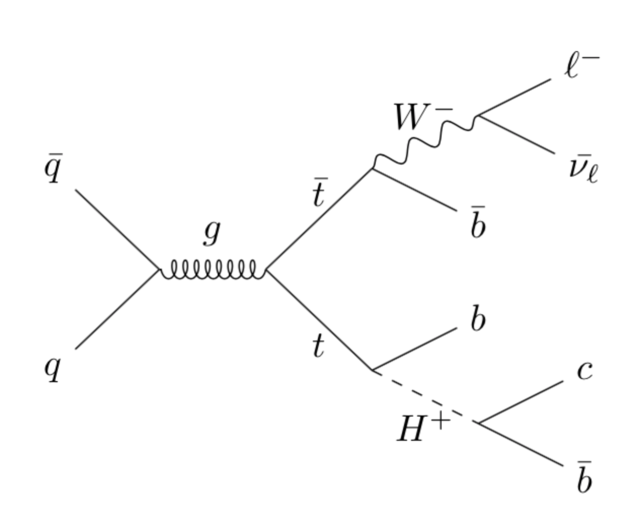
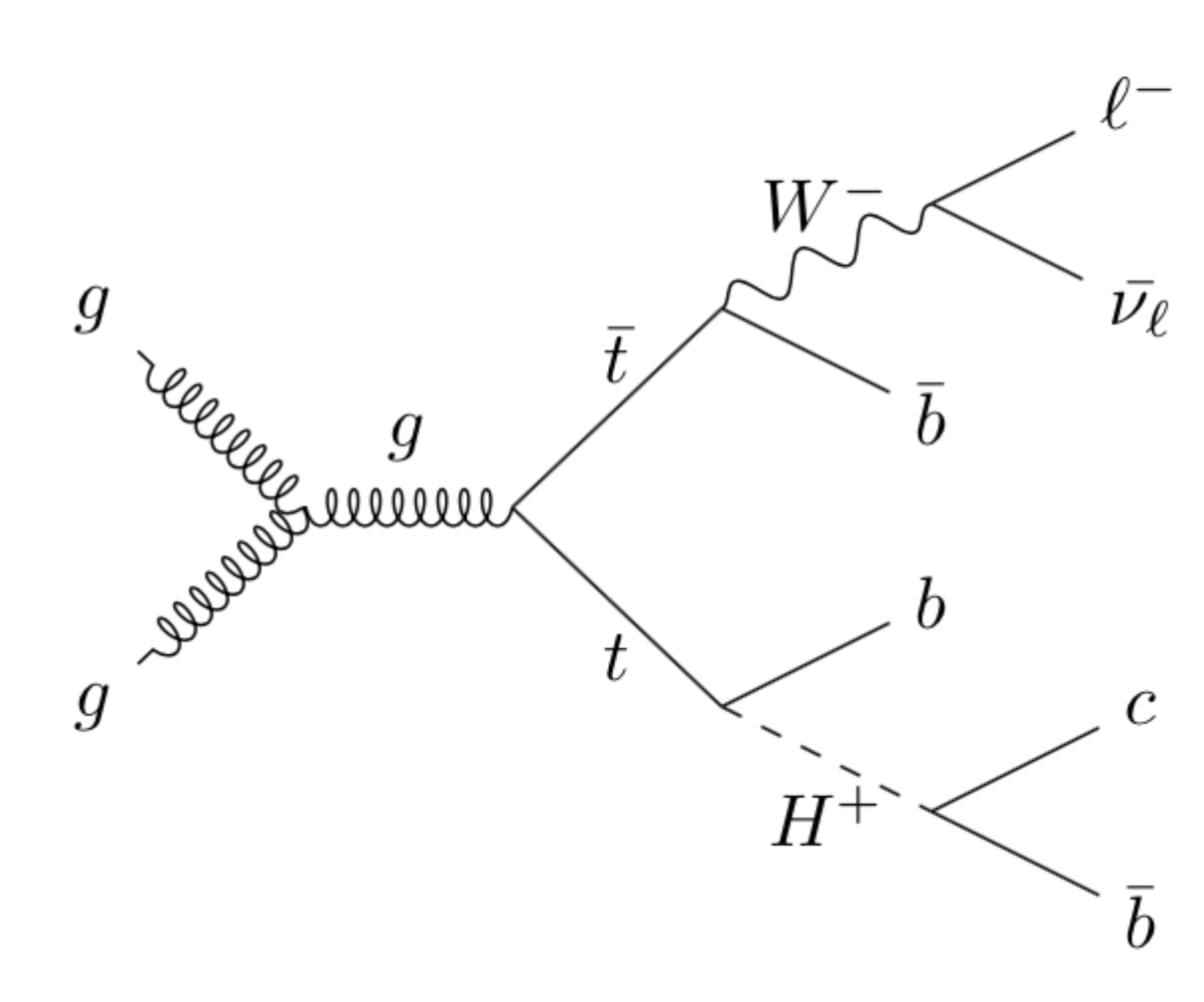
This paper presents a search for $H^{\pm}\rightarrow cb$ in top-quark decays which is based on a dataset of $pp$ collisions collected at a centre-of-mass energy $\sqrt{s}=13\;\text{TeV}$ between 2015 and 2018 with the ATLAS detector, amounting to an integrated luminosity of 139 fb^-1. The analysis focuses on a data sample enriched in top-quark pair production ($t\bar{t}$), where one top quark decays into a leptonically decaying $W$ boson and a bottom quark, and the other top quark decays into a $H^{\pm}$ boson and a bottom quark, as illustrated in Figure 1. Compared to searches for $H^{\pm}\rightarrow cs$ and $H^{\pm}\rightarrow\tau\nu$ in $t\bar{t}$ events, searches for $H^{\pm}\rightarrow cb$ take advantage of a significantly smaller yield of the irreducible SM background originating from $t\bar{t}$ production with a $W$ boson decaying into the Cabibbo–Kobayashi–Maskawa suppressed mode $W\rightarrow cb$. The search exploits the high multiplicity of jets containing $b$-hadrons ($b$-jets), as expected from signal events, and deploys a neural network classifier that uses the kinematic differences between the signal and the background. Thanks to a sizeably larger dataset and improved analysis techniques, this search improves the expected sensitivity to $H^{\pm}\rightarrow cb$ in top-quark decays by a factor of five compared to the previous publication [23] and explores an extended $m_{{H}^{\pm}}$ range, between 60 and 160 GeV.

Figure 1: Illustrative leading-order Feynman diagrams for the signal considered. Charge-conjugated Feynman diagrams are also assumed.

2 ATLAS detector

The ATLAS experiment [26] at the LHC is a multipurpose particle detector with a forward–backward symmetric cylindrical geometry and a near $4\pi$ coverage in solid angle. It consists of an inner tracking detector surrounded by a thin superconducting solenoid providing a $2\text{\,}\mathrm{T}$ axial magnetic field, electromagnetic and hadron calorimeters, and a muon spectrometer. The inner tracking detector covers the pseudorapidity range $|\eta|<2.5$. It consists of silicon pixel, silicon microstrip, and transition radiation tracking detectors. Lead/liquid-argon (LAr) sampling calorimeters provide electromagnetic (EM) energy measurements with high granularity. A steel/scintillator-tile hadron calorimeter covers the central pseudorapidity range ($|\eta|<1.7$). The endcap and forward regions are instrumented with LAr calorimeters for both the EM and hadronic energy measurements up to $|\eta|=4.9$. The muon spectrometer surrounds the calorimeters and is based on three large superconducting air-core toroidal magnets with eight coils each. The field integral of the toroids ranges between $2.0$ and $6.0\text{\,}\mathrm{T}\text{\,}\mathrm{m}$ across most of the detector. The muon spectrometer includes a system of precision tracking chambers and fast detectors for triggering. A two-level trigger system is used to select events. The first-level trigger is implemented in hardware and uses a subset of the detector information to accept events at a rate below $100\text{\,}\mathrm{kHz}$. This is followed by a software-based trigger that reduces the accepted event rate to $1\text{\,}\mathrm{kHz}$ on average depending on the data-taking conditions. An extensive software suite [27] is used for real and simulated data reconstruction and analysis, for operation and in the trigger and data acquisition systems of the experiment.

3 Objects definition and event selection

Data from $pp$ collisions at $\sqrt{s}=13\,\text{TeV}$ were recorded by the ATLAS detector between 2015 and 2018. Only data for which all detector subsystems were operational are used [28]; this dataset corresponds to an integrated luminosity of 139 fb^-1 [29, 30].

Events were recorded with a single-electron or single-muon trigger, with minimum thresholds for the transverse momentum ($p_{\text{T}}$) varying from 20 to 26 GeV  depending on the lepton flavour and the data-taking period. The triggers with the lowest $p_{\text{T}}$ thresholds included isolation requirements based on the inner tracking detector or electromagnetic calorimeter measurements [31, 32, 33, 34].

In each event, the primary vertex is defined as the reconstructed vertex having the highest scalar sum of the squared $p_{\text{T}}$ of associated tracks with $p_{\text{T}}\geq 0.5$ GeV.

Electrons are reconstructed from energy clusters in the electromagnetic calorimeter that are geometrically matched to a track in the inner tracking detector. Electrons are required to satisfy $|\eta|<2.47$ and a ‘Tight’ identification requirement using a likelihood-based method [35]; electrons are rejected if their calorimeter clusters lie within the transition region between the barrel and endcaps of the electromagnetic calorimeter, $1.37<|\eta|<1.52$. Muons are reconstructed from muon spectrometer tracks matched to tracks in the inner tracking detector in the pseudorapidity range $|\eta|<2.5$. Muon identification is based on ‘Medium’ requirements [36]. Selected electrons and muons are required to have $p_{\text{T}}\geq 27$ GeV.

Isolation criteria are applied to the selected electrons and muons. For electrons, the scalar sum of the transverse energy in calorimeter energy clusters within a cone of size $\Delta R=0.2$ around the electron is required to be less than 6% of the electron $p_{\text{T}}$, excluding clusters originating from the electron itself. For muons, the scalar sum of the $p_{\text{T}}$ of tracks within a fixed-size cone around the muon (excluding its associated track) must be less than 6% of the muon $p_{\text{T}}$. The track isolation cone size is $\Delta R=0.3$ for muon $p_{\text{T}}<50$ GeV and $\Delta R=0.2$ for muon $p_{\text{T}}>50$ GeV.

Jets are reconstructed from topological energy clusters in the calorimeter [37] using the particle-flow method [38], based on the anti-$k_{t}$ clustering algorithm [39, 40] with a radius parameter of $0.4$. The jet energy is calibrated at particle level [41], and jets are required to have $|\eta|<2.5$ and a minimum $p_{\text{T}}$ of 25 GeV. For jets with $|\eta|<2.4$ and $p_{\text{T}}<60$ GeV, those originating from additional $pp$ collisions in the same or neighbouring bunch crossings (pile-up) are suppressed by the use of the ‘jet-vertex-tagger’ [42].

Jets containing $b$-hadrons are identified with the DL1r $b$-tagging algorithm [43]. A jet is $b$-tagged if the DL1r score is above a certain threshold, referred to as an operating point (OP). Four OPs are defined with average expected efficiencies for $b$-jets of 60%, 70%, 77% and 85%, as determined in simulated $t\bar{t}$ events. The DL1r $b$-tagging score is divided into five exclusive bins according to the OPs. The distribution obtained by ordering these five bins from higher to lower $b$-jet efficiency is referred to as the ‘pseudo-continuous’ $b$-tagging score.

The missing transverse momentum, with magnitude $E_{\text{T}}^{\text{miss}}$, is defined as the negative vector sum of the transverse momenta of all selected and calibrated physics objects. Low-momentum tracks from the primary vertex that cannot be associated with any of the reconstructed physics objects described before are also included in the $E_{\text{T}}^{\text{miss}}$ calculation [44].

A sequential overlap removal procedure is applied to ensure that the same calorimeter energy deposit or the same track is not associated with two or more different reconstructed objects, following the prescription described in Ref. [45].

The events are required to have exactly one selected electron or muon that matches the lepton that fired the trigger, and at least four jets. At least two of the jets are required to pass the 60% OP $b$-tagging requirement and an additional jet is required to pass the 70% $b$-tagging OP. In order to suppress background from multijet production, additional requirements are made on $E_{\text{T}}^{\text{miss}}$ as well as on the transverse mass of the lepton and $E_{\text{T}}^{\text{miss}}$ system ($m_{\text{T}}^{W}$): $E_{\text{T}}^{\text{miss}}>20\leavevmode\nobreak\ \text{GeV}$ and $E_{\text{T}}^{\text{miss}}+m_{\text{T}}^{W}>60\leavevmode\nobreak\ \text{GeV}$. The above requirements are referred to as the “preselection”.

4 Monte Carlo samples

Monte Carlo (MC) simulation samples are used to model all backgrounds as well as the $H^{\pm}$ signal, and evaluate related modelling uncertainties. The main background for this search originates from $t\bar{t}$ production in association with jets, followed by smaller contributions from single-top-quark, $V$+jets, $t\bar{t}V$, $t\bar{t}H$, diboson and other rare processes involving the production of a top quark. Background due to non-prompt leptons is expected to be negligible, based on studies of data using multiple lepton isolation criteria [46] and analysis of low-$E_{\text{T}}^{\text{miss}}$ events.

The matrix-element calculations for all generated samples use the NNPDF3.0nlo [47] set of parton distribution functions (PDFs), unless stated otherwise. In all samples interfaced to Pythia 8 [48] or Herwig 7 [49, 50], the decays of bottom and charm hadrons were simulated using the EvtGen 1.2.0 program [51]. Pythia 8.230 [52] modelled the parton shower, hadronisation, and underlying event, with parameters set according to the A14 tune [53] and using the NNPDF2.3lo [47] PDF set; Herwig 7.04 used the H7UE tune and the MMHT2014lo [54] PDF set; and Herwig 7.13 used the Herwig 7.1 default set of tuned parameters and the same PDF set. The effect of pile-up was modelled by overlaying each simulated hard-scatter event with inelastic $pp$ events generated with Pythia 8.186 using the NNPDF2.3lo [55] PDF set and the A3 tune [56].

The generated events were processed through either a simulation [57] of the ATLAS detector geometry and response using Geant4 [58] or a faster simulation, where the full Geant4 simulation of the calorimeter response is replaced by a detailed parameterisation of the shower shapes [59]. Simulated events were processed through the same reconstruction software as the data, and corrections were applied so that the object identification efficiencies, energy scales and energy resolutions matched those determined from data control samples.

4.1 $t\bar{t}$ background simulation

The production of $t\bar{t}\rightarrow WbWb$ events (denoted simply $t\bar{t}$ in the following) was modelled using the Powheg Box v2 [60, 61, 62, 63] generator at next-to-leading order (NLO) with the $h_{\mathrm{damp}}$ parameter set to 1.5 times the top-quark mass, $m_{\text{top}}$ [64]. The matrix-element calculation includes diagrams with a $b$-quark in the initial state using the five-flavour scheme [65]. The events were interfaced to Pythia 8.230 [52] to model the parton shower, hadronisation, and underlying event.

The impact of using a different parton shower and hadronisation model was evaluated by comparing the nominal $t\bar{t}$ sample with another sample produced with the Powheg Box v2 generator interfaced to Herwig 7.04 instead of Pythia 8.230.

To assess the uncertainty associated with the NLO generator, the Powheg Box v2 sample was compared with a sample of events generated with MadGraph5_aMC@NLO 2.6.0 interfaced to Pythia 8.230.

Analogously to similar searches performed previously in ATLAS [66, 46], the simulated $t\bar{t}$ events are categorised according to the flavour content of additional jets not originating from the decay of the $t\bar{t}$ system. Events that have at least one $b$-jet, excluding heavy-flavour jets from top-quark or $W$-boson decays, are labelled as $t\bar{t}$+$\geq$1b; those with no additional $b$-jets but at least one charm-jet ($c$-jet) are labelled as $t\bar{t}$+$\geq$1c; finally, events not containing any additional heavy-flavour jets are labelled as $t\bar{t}$+light.

An additional sample to evaluate systematic uncertainties in the modelling of the $t\bar{t}$+$\geq$1b process was produced with the Powheg Box Res [67] generator and OpenLoops [68, 69, 70], using a pre-release of the implementation of this process in Powheg Box Res provided by its authors [71]. It was interfaced to Pythia 8.240. The four-flavour scheme was used with the $b$-quark mass set to 4.95 GeV. The factorisation scale was set to $0.5\times\Sigma_{i=t,\bar{t},b,\bar{b},j}m_{\mathrm{T},i}$, where $m_{\mathrm{T},i}=(m_{i}^{2}+p_{\text{T},i}^{2})^{1/2}$ and $j$ denotes extra light quarks or gluons, the renormalisation scale was set to $\prod_{i=t,\bar{t},b,\bar{b}}m_{\mathrm{T},i}^{1/4}$, and the $h_{\mathrm{damp}}$ parameter was set to $0.5\times\Sigma_{i=t,\bar{t},b,\bar{b}}m_{\mathrm{T},i}$.

All generated $t\bar{t}$ samples assume a diagonal Cabibbo–Kobayashi–Maskawa matrix, thus neglecting $t\bar{t}$ events with rare $W\rightarrow cb$ decays. Since such decays mimic the expected topology of the $H^{\pm}\rightarrow cb$ signal, dedicated $t\bar{t}$ samples were produced, setting $V_{cb}=0.041$. A nominal sample was generated by using Powheg Box v2 at NLO with the $h_{\mathrm{damp}}$ parameter set to $1.5\times m_{\text{top}}$, and using MadSpin [72, 73] to generate $W\rightarrow cb$ decays. The events were interfaced to Pythia 8.230 to model the parton shower, hadronisation, and underlying event. Additional samples to assess the uncertainty in the parton shower and hadronisation model and the NLO generator were produced with Powheg Box v2 interfaced to Herwig 7.13 and MadGraph5_aMC@NLO 2.6.0 interfaced to Pythia 8.230.

The $t\bar{t}$ sample was normalised to the cross-section prediction at next-to-next-to-leading order (NNLO) in QCD including the resummation of next-to-next-to-leading logarithmic (NNLL) soft-gluon terms calculated using Top++ 2.0 [74, 75, 76, 77, 78, 79, 80]. For $pp$ collisions at a centre-of-mass energy of $\sqrt{s}$ = $13\text{\,}\mathrm{TeV}$, this cross-section corresponds to $\sigma(t\bar{t})=\mathrm{832\pm 51\leavevmode\nobreak\ pb}$ using a top-quark mass of $m_{\text{top}}=172.5\,\text{GeV}$.

4.2 Signal simulation

Samples of $t\bar{t}\rightarrow H^{\pm}bW^{\mp}b$ events were generated using the Powheg Box v2 generator at NLO with the $h_{\mathrm{damp}}$ parameter set to $1.5\times m_{\text{top}}$, and using MadSpin and Pythia 8.230 to perform the top quark and $H^{\pm}\rightarrow cb$ decays and to model the parton shower, hadronisation, and underlying event. The $W$ boson was forced to decay leptonically to all three lepton flavours. A total of 11 signal MC samples were generated with $m_{{H}^{\pm}}$ ranging from 60 to 160 GeV with 10 GeV spacing; the $H^{\pm}$ boson’s total width is assumed to be 1 GeV, more than ten times smaller than the expected mass resolution. The signal samples were normalised to the same cross-section as used for the $t\bar{t}$ background sample, and assuming an arbitrary product of branching fractions $\mathscr{B}_{\text{ref}}=\mathscr{B}(t\rightarrow H^{\pm}b)\,\times\mathscr{B}(H^{\pm}\rightarrow cb)=1\%$.

4.3 Other samples

The associated production of top quarks with $W$ bosons ($tW$) and single-top-quark production in the $t$-channel and $s$-channel were modelled by the Powheg Box v2 generator at NLO in QCD using the five-flavour scheme. The $tW$ process was modelled using the diagram removal scheme [81, 82] to handle interference and overlap with $t\bar{t}$ production. A related uncertainty was estimated by comparison with an alternative sample generated using the diagram subtraction scheme [81, 82]. The events were interfaced to Pythia 8.230. The uncertainty due to the parton shower and hadronisation model was evaluated by comparing the nominal samples of events with samples where events generated with Powheg Box v2 were interfaced to Herwig 7.04 instead of Pythia 8.230. To assess the uncertainty associated with the NLO generator, the nominal samples were compared with samples generated with MadGraph5_aMC@NLO 2.6.2 at NLO in QCD using the five-flavour scheme and the NNPDF2.3nlo PDF set. These events were interfaced to Pythia 8.230.

For the $tW$ channel single-top-quark process, the inclusive cross-section was normalised to the theory prediction calculated at NLO in QCD with NNLL soft-gluon corrections [83, 84]. The inclusive cross-section for $t$-channel and $s$-channel single-top-quark production was calculated at NLO in QCD with Hathor 2.1 [85, 86].

The $V+$jets ($V=W,Z$) and the diboson ($WW$, $WZ$, $ZZ$) production was simulated with the Sherpa 2.2.1 or 2.2.2 generator [87] depending on the process. The simulation of $V+$jets used the NLO matrix elements for up to two partons, and leading-order (LO) matrix elements for up to four partons, calculated with the Comix [88] and OpenLoops libraries. The diboson samples, including fully leptonic final states and semileptonic final states, where one boson decays leptonically and the other hadronically, were generated using matrix elements at NLO accuracy in QCD for up to one additional parton and at LO accuracy for up to three additional parton emissions; off-shell effects and Higgs boson contributions are accounted for, where appropriate. The calculations were matched with the Sherpa parton shower [89] using the MEPS@NLO prescription [90, 91, 92, 93], The NNPDF3.0nnlo set of PDFs was used for the matrix-element calculation, along with the dedicated set of tuned parton-shower parameters developed by the Sherpa authors. The $V+$jets samples were normalised to a NNLO prediction [94].

The production of $t\bar{t}H$ events was modelled using the Powheg Box v2 generator at NLO. The events were interfaced to Pythia 8.230. The impact of using a different parton shower and hadronisation model was evaluated by showering the nominal hard-scatter events with Herwig 7.04. To assess the uncertainty associated with the NLO generator, the nominal samples were compared with samples generated with MadGraph5_aMC@NLO 2.6.2 at NLO in QCD using the five-flavour scheme and the NNPDF2.3nlo PDF set; these events were interfaced to Pythia 8.230. The $t\bar{t}H$ cross-section was calculated at NLO QCD and NLO electroweak accuracies using MadGraph5_aMC@NLO as reported in Ref. [95].

The production of $t\bar{t}V$ and $tHq$ events was modelled at NLO using the MadGraph5_aMC@NLO 2.3.3 generator interfaced to Pythia 8.210.

The production of $tZq$ events was modelled using the MadGraph5_aMC@NLO 2.3.3 generator at LO. The events were interfaced to Pythia 8.210. The $tZq$ total cross-section was calculated at NLO using MadGraph5_aMC@NLO 2.3.3 with the NNPDF3.0nlo PDF set.

5 Analysis strategy

This section presents an overview of the analysis strategy developed for the $H^{\pm}\rightarrow cb$ search; it closely follows that of similar searches performed previously by ATLAS [66, 96].

5.1 Event categorisation

This search targets the production of a charged Higgs boson via top-quark-pair decay, $t\bar{t}\rightarrow H^{\pm}bW^{\mp}b$, followed by the decays $H^{\pm}\rightarrow cb$ and $W^{\mp}\rightarrow\ell\nu$, where $\ell$ denotes an electron or muon. The resulting signal event topology is characterised by four jets in the final state, three of them originating from $b$-quarks and one from a $c$-quark, which can be effectively exploited to suppress the background. Additional jets can also be present because of initial- or final-state radiation.

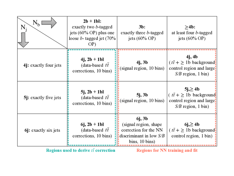
In order to maximise the sensitivity of the search, the preselected events are categorised into different analysis regions depending on the number of jets (4, 5 and 6) and on the number of $b$-tagged jets (3 and $\geq$4); they are summarised in Figure 2. Events with two $b$-tagged jets are retained only if they have an additional $b$-tagged jet selected with a looser requirement: they satisfy the 70% OP but fail the nominal (i.e. 60%) OP (denoted 2b+1bl). Therefore, a total of nine analysis regions are considered: (4j, 2b+1bl), (5j, 2b+1bl), (6j, 2b+1bl), (4j, 3b), (5j, 3b), (6j, 3b), (4j, 4b), (5j, $\geq$4b) and (6j, $\geq$4b), where ($n$j, $m$b + $k$bl) indicates $n$ selected jets, among which $m$ and $k$ are $b$-tagged with the nominal and loose $b$-tagging requirements, respectively; event categories with at least three $b$-tagged jets passing the 60% OP are used in the statistical analysis and thus are referred to as ‘fit regions’.

As explained in Section 5.2, the 2b+1bl regions are used to derive data-based corrections to improve the modelling of the $t\bar{t}$ background. The definition of these analysis regions ensures a background composition as close as possible to what is expected in fit regions with three $b$-tagged jets. The main signal regions are (4j, 3b) and (5j, 3b); for $\mathscr{B}=0.1\%$, the signal purity in these regions can reach a maximum value over the explored $m_{{H}^{\pm}}$ range of 2.8% for the former and 1.9% for the latter. The (6j, 3b) region has lower signal purity, below 1.3% for $\mathscr{B}=0.1\%$, and it is used mainly to constrain the background modelling uncertainties via a profile-likelihood fit (see Section 7). Finally, the (5j, $\geq$4b) and (6j, $\geq$4b) regions offer a clean control sample to calibrate the $t\bar{t}$+$\geq$1b background, while data belonging to the (4j, 4b) region are used to recover acceptance for signal events with a $c$-quark misidentified as a $b$-jet.

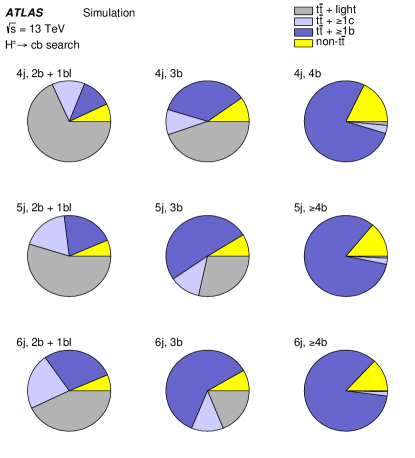
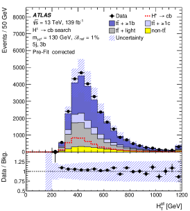
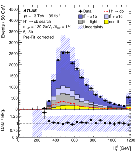
Figure 3 shows the fractions of the different background components in the analysis regions. In all regions, $t\bar{t}$ production is the main source of SM background; it accounts for more than 80% of the expected background. The $t\bar{t}$ background composition depends on the jet and $b$-jet multiplicities. Analysis regions that include a 2b+1bl requirement have a background composition consisting of up to 62% $t\bar{t}$+light and up to 28% $t\bar{t}$+$\geq$1b, with an increasing fraction of $t\bar{t}$+$\geq$1b at higher jet multiplicity. The fit regions with a 3b requirement have higher fraction of $t\bar{t}$+$\geq$1b background, up to 61%. Most of the $t\bar{t}$+light background events in these regions have a $b$-tagged $c$-jet from the hadronic $W$-boson decay, in addition to the two $b$-jets from the top-quark decays. The background in regions with the $\geq$4b requirement is mostly $t\bar{t}$+$\geq$1b. The $t\bar{t}$+$\geq$1c and other backgrounds are small in all analysis regions; the $t\bar{t}$+$\geq$1c background mostly populates the 2b+1bl regions, accounting for up to 22% of the expected SM background contribution. Non-$t\bar{t}$ production contributes up to 13% in any analysis region.

Figure 2: Summary of the analysis regions along with information about their usage, as described in the text. The $b$-tagging selection is based on the DL1r algorithm’s 60$\%$ efficiency OP.

Figure 3: Fractional contributions of the various processes to the total background prediction in each analysis region. The small contributions from $t\bar{t}V$, $t\bar{t}H$, single-top-quark, $W/Z$+jets, diboson, $tHq$ and $tZq$ backgrounds are combined into a single background source referred to as “non-$t\bar{t}$”. The predictions for the various background contributions are obtained through the simulation as described in Section 4.

5.2 $t\bar{t}$ modelling

The main background for this search originates from $t\bar{t}$ production in association with jets. It was observed that the $t\bar{t}$ simulation does not provide a fully satisfactory description of the jet multiplicity and transverse energy distributions in data; this motivates the introduction of a data-based approach to correct the $t\bar{t}$ simulation, similar to that developed in recent ATLAS searches [46, 97].

The data and the SM prediction are compared in the 2b+1bl regions separately for events with four, five or six jets. In these three analysis regions, independent corrections for the $t\bar{t}$ simulation are derived as a function of $H_{\mathrm{T}}^{\mathrm{all}}$, which is defined as the scalar sum of the transverse momenta of all selected objects in the event and $E_{\text{T}}^{\text{miss}}$.

The correction factor in a given $H_{\mathrm{T}}^{\mathrm{all}}$ bin ($H_{\mathrm{T}}^{\mathrm{all,\,i}}$) and jet multiplicity region (jⁱ) is defined as

$$C(H_{\mathrm{T}}^{\mathrm{all,\,i}},\;\text{j}^{i})=\frac{N^{\text{data}}(H_{\mathrm{T}}^{\mathrm{all,\,i}},\;\text{j}^{i})-N^{\text{non-$t\bar{t}$}}(H_{\mathrm{T}}^{\mathrm{all,\,i}},\;\text{j}^{i})}{N^{\text{$t\bar{t}$}}(H_{\mathrm{T}}^{\mathrm{all,\,i}},\;\text{j}^{i})}$$

where $N^{\text{data}}(H_{\mathrm{T}}^{\mathrm{all,\,i}},\;\text{j}^{i})$, $N^{\text{non-$t\bar{t}$}}(H_{\mathrm{T}}^{\mathrm{all,\,i}},\;\text{j}^{i})$ and $N^{\text{$t\bar{t}$}}(H_{\mathrm{T}}^{\mathrm{all,\,i}},\;\text{j}^{i})$ represent respectively the yields observed in data, and the predicted non-$t\bar{t}$ and $t\bar{t}$ yields in the $H_{\mathrm{T}}^{\mathrm{all}}$ bin and jet multiplicity under consideration. The non-$t\bar{t}$ yields include the small contributions from $t\bar{t}V$, $t\bar{t}H$, single-top-quark, $W/Z$+jets, diboson, $tHq$ and $tZq$ backgrounds. The fraction of subtracted non-$t\bar{t}$ background is about 7.1% in the (4j, 2b+1bl) region, 6.4% in the (5j, 2b+1bl) region, and 6.4% in the (6j, 2b+1bl) region. In all jet multiplicities, the derived corrections are close to unity for $H_{\mathrm{T}}^{\mathrm{all}}$ above 800 GeV, and increase monotonically towards lower $H_{\mathrm{T}}^{\mathrm{all}}$ values, reaching 1.2 for $H_{\mathrm{T}}^{\mathrm{all}}=200$ GeV. The corrections are parameterised as a function of $H_{\mathrm{T}}^{\mathrm{all}}$ in each jet multiplicity bin using rational functions of varying degree. A possible signal contamination in the 2b+1bl regions would mostly result in a normalisation offset for the $t\bar{t}$ prediction, smaller than 1.5%, due to the similarity of the $t\bar{t}$ background and signal $H_{\mathrm{T}}^{\mathrm{all}}$ distribution shapes. Such an effect is fully absorbed by the systematic uncertainties of the $t\bar{t}$ prediction and has a numerically negligible impact on the signal extraction.

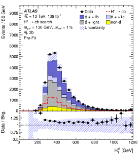
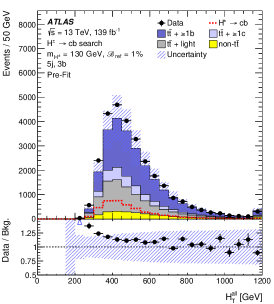
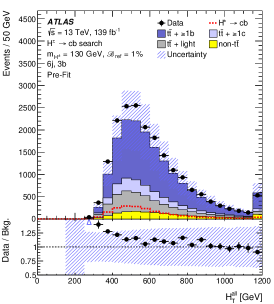
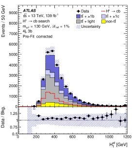
It was verified that after the inclusion of the data-based $t\bar{t}$ corrections there is a consistently better agreement between data and the SM prediction in all analysis regions and for a wide range of observables. Figure 4 compares the $H_{\mathrm{T}}^{\mathrm{all}}$ distribution of data events with that of the background prediction before and after applying the data-based correction to the $t\bar{t}$ background simulation in analysis regions with three $b$-tagged jets that contain events not used to derive the $t\bar{t}$ corrections. An improved agreement between the background prediction and data is observed, despite the fact that the correction was derived in a region with substantially lower $t\bar{t}$+$\geq$1c and $t\bar{t}$+$\geq$1b fractions (see Fig. 3). This demonstrates the appropriateness of applying these corrections to all $t\bar{t}$ components ($t\bar{t}$+light, $t\bar{t}$+$\geq$1c, and $t\bar{t}$+$\geq$1b) in the simulation. To account for residual differences in their modelling, the associated systematic uncertainties are treated as uncorrelated between the three $t\bar{t}$ components (see Sect. 6.3).

((a))

((b))

((c))

((d))

((e))

((f))

Figure 4: Comparison between the data and prediction for the $H_{\mathrm{T}}^{\mathrm{all}}$ distribution (a-c) before and (d-f) after the inclusion of the data-based $t\bar{t}$ correction (“corrected”), in regions with three $b$-tagged jets prior to the likelihood fit to data (“Pre-Fit”), see Section 7. The small contributions from $t\bar{t}V$, $t\bar{t}H$, single-top-quark, $W/Z$+jets, diboson, $tHq$ and $tZq$ backgrounds are combined into a single background source referred to as “non-$t\bar{t}$”. The expected $H^{\pm}$ signal for $m_{{H}^{\pm}}$ = 130 GeV is displayed as a dashed red line normalised to $\mathscr{B}_{\text{ref}}=1\%$. The bottom panels display the ratios of data to the SM background prediction (“Bkg.”) before the likelihood fit. The hashed area represents the total uncertainty of the background. The last bin in all figures contains the overflow.

5.3 Neural network discriminant

A feed-forward neural network is used to separate the $H^{\pm}$ signal from the large SM background. The neural network input layer receives kinematic information about reconstructed objects, invariant masses of jet-pair permutations, and pseudo-continuous $b$-tagging scores, for a total of 29 input variables, summarised in Table 1. The selected jets are initially sorted according to their pseudo-continuous $b$-tagging scores. For jets with degenerate $b$-tagging scores a $p_{\text{T}}$ ordering is applied. After the jet ordering, the fourth jet in signal events is expected to originate from the charm-quark produced in the $H^{\pm}$ decays. The neural network uses the $p_{\text{T}}$, $\eta$ and $\phi$ of the first six sorted jets along with the $b$-tagging score for the fourth, fifth and sixth jets. These kinematic distributions and their correlations allow the signal to be distinguished from SM background by considering the resonances produced in the event, while the $b$-tagging scores are effective in distinguishing the three $t\bar{t}$ background components ($t\bar{t}$+light, $t\bar{t}$+$\geq$1b and $t\bar{t}$+$\geq$1c) from the signal. The $p_{\text{T}}$, $\eta$, and $\phi$ of the lepton, as well as $E_{\text{T}}^{\text{miss}}$ and its $\phi$ angle, are also included to fully characterise the event kinematics. Finally, three dijet invariant masses correlated with $m_{{H}^{\pm}}$ are obtained by calculating the invariant mass of each of the three leading jets and the fourth jet; the inclusion of these invariant mass distributions improves the neural network’s separation of signal from background by about 20%.

Table 1: List of input variables used in the neural network training. Jets are sorted according to their pseudo-continuous $b$-tagging scores, followed by their $p_{\text{T}}$, in case of having the same score.

Input variables	Number of variables
$p_{\text{T}}$, $\eta$, and $\phi$ of the first six leading jets	18
$b$-tagging score of the fourth, fifth, and sixth jets	3
Lepton $p_{\text{T}}$, $\eta$, and $\phi$	3
Missing transverse energy and its $\phi$ angle	2
Invariant mass between each of the three leading jets and the fourth jet	3
Total	29

The neural network input layer is followed by fully connected hidden layers using rectified-linear-unit activation functions; a sigmoid function is then used in the output layer. Batch normalisation [98] is applied before each hidden layer. The training uses the Adam optimiser [99] in combination with four-fold cross-training [100], which provides orthogonal data samples for the optimisation of the neural network hyperparameters. The best hyperparameter configuration includes 2 layers and 190 neurons. The impact of overtraining is mitigated with the ‘dropout’ [101] method in combination with the ‘MaxNorm’ constraint.

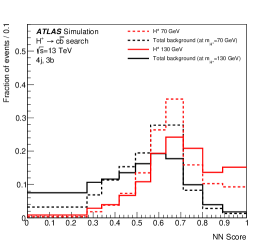
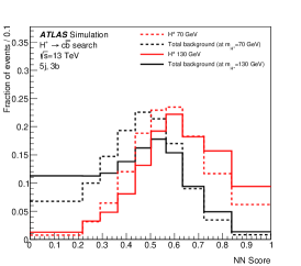
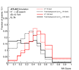
The neural network is trained by using events with exactly four, five or six jets, and at least three $b$-tagged jets, corresponding to the analysis regions with highest signal purity. The training also includes the value of the $m_{{H}^{\pm}}$ parameter, which for signal events is defined to be the true mass of the signal sample. In the case of background events, a random value of the $H^{\pm}$ mass, taken from the fraction of signal masses in the input dataset, is assigned to each event [102]. In addition to increasing the size of the training sample, the use of a mass-parameterised neural network allows the different signals to be differentiated. Figure 5 compares the distributions of the neural network output score (‘NN score’) of the $H^{\pm}$ signal, for $m_{{H}^{\pm}}=70$ GeV and $m_{{H}^{\pm}}=130$ GeV, and the total SM background in the three most sensitive regions, (4j, 3b), (5j, 3b) and (6j, 3b).

((a))

((b))

((c))

Figure 5: Comparison of the distributions of the NN score of the $H^{\pm}$ signal with $m_{{H}^{\pm}}=70$ GeV (red dashed) and $m_{{H}^{\pm}}=130$ GeV (red solid), and the total SM background evaluated at the same masses (black dashed and black solid, respectively) in the analysis regions (a) (4j, 3b), (b) (5j, 3b), and (c) (6j, 3b). Each NN score distribution is normalised to unit area.

6 Systematic uncertainties

Several sources of systematic uncertainty can affect the normalisation of the signal and backgrounds, as well as the shape of their corresponding NN scores distributions. Each source of systematic uncertainty is considered to be uncorrelated with the other sources. Correlations for a given systematic uncertainty are maintained across processes and event categories, unless explicitly otherwise stated. The following sections describe the considered systematic uncertainties.

6.1 Luminosity and pile-up

The uncertainty in the measurement of the integrated luminosity of the used dataset is 1.7% [29]; it affects the overall normalisation of all processes estimated from the simulation. The uncertainty is derived using the LUCID-2 detector for the baseline luminosity measurements [30], from a calibration of the luminosity scale using $x$–$y$ beam-separation scans.

An uncertainty is assigned to the modelling of pile-up in simulation to account for differences between the predicted and measured inelastic cross-sections in a given fiducial volume [103].

The uncertainties in the luminosity measurement and pile-up modelling are treated as being correlated across the analysis regions and all physics processes.

6.2 Object reconstruction

Uncertainties associated with electrons and muons arise from the trigger, reconstruction, identification and isolation efficiencies, as well as the momentum scale and resolution [36, 35, 31, 32]. They are measured using data enriched in $Z\to\ell^{+}\ell^{-}$ and $J/\psi\to\ell^{+}\ell^{-}$ events ($\ell=e,\mu$). Uncertainties in jet measurements arise from the jet energy scale and resolution, and the efficiency to pass the jet-vertex-tagger requirements [104, 42]. The largest contribution comes from the jet energy scale, the uncertainty of which is split into 29 uncorrelated components, and depends on jet $p_{\text{T}}$ and $\eta$, jet flavour, pile-up treatment, and simulation of the hadronic shower shape. The jet energy scale is calibrated with a series of simulation-based corrections and measurements in data samples enriched in photon or $Z$ boson production in association with jets or in multijet production.

Uncertainties associated with energy scales and resolutions of leptons and jets are propagated to the $E_{\text{T}}^{\text{miss}}$ reconstruction. Additional uncertainties affecting the reconstruction of low-energy particles present in the event, not associated with any leptons or jets, are measured in $Z\to\ell^{+}\ell^{-}$ data by studying the recoil of the $Z$ boson [44].

Efficiencies to tag jets in the simulation are corrected to match the efficiencies measured in data by applying $p_{\text{T}}$-dependent factors. The $b$-jet efficiencies and $c$-jet mis-tagging rates are measured in a data sample enriched in $t\bar{t}$ events [105, 106] , while the light-jet mis-tagging rates are measured in a multijet data sample enriched in light-jets [107]. Uncertainties affecting $b$-, $c$-, and light-jet efficiencies or mis-tagging rates are decomposed into 45, 15 and 20 uncorrelated components, respectivly.

All uncertainties affecting object reconstruction are treated as being correlated across the analysis regions and all physics processes, including signal.

6.3 $t\bar{t}$ background modelling

The systematic uncertainties assigned to the $t\bar{t}$ background are designed to cover potential mismodelling of this background as a function of jet and $b$-jet multiplicities. Since the diagrams that contribute to $t\bar{t}$+$\geq$1b, $t\bar{t}$+$\geq$1c, and $t\bar{t}$+light processes are different, their associated uncertainties are treated as being uncorrelated from each other, unless otherwise stated.

Uncertainties associated with the choice of matrix-element generator and parton shower and hadronisation models are obtained by comparing the nominal $t\bar{t}$  sample with alternative samples described in Section 4. These uncertainties are evaluated in a consistent way by first putting the alternative $t\bar{t}$ samples through the same data-based correction procedure utilised to correct the nominal $t\bar{t}$ sample (Section 5.2). The $t\bar{t}$ modelling uncertainties are then evaluated by comparing the alternative $t\bar{t}$ samples with the nominal samples, both sets having had the data-based correction applied. These uncertainties are also decorrelated between different jet multiplicity regions.

The uncertainty due to initial- and final-state radiation (ISR/FSR) was estimated by varying the parameters of the A14 parton shower tune [108] as described in Ref. [97]. Uncertainties accounting for missing higher-order QCD corrections in the matrix-element calculation are estimated by varying the renormalisation and factorisation scales in Powheg Box v2 independently by factors of 2 and 0.5 relative to the nominal scales choice. Uncertainties due to higher-order QCD corrections and ISR/FSR modelling are treated as being correlated between different jet multiplicity regions.

A normalisation uncertainty of $50\%$ is assumed separately for $t\bar{t}$+$\geq$1b and $t\bar{t}$+$\geq$1c. For $t\bar{t}$+$\geq$1c, the uncertainty choice is conservative given the ability to determine this background from data and the very limited sensitivity of the final results to this choice. In the case of $t\bar{t}$+$\geq$1b, this choice is motivated by the observed level of disagreement between data and prediction for this background [109].

Systematic uncertainties in the data-based $t\bar{t}$ corrections arise from the statistical uncertainty in the parameterisation of the correction factors and subtraction of the non-$t\bar{t}$ backgrounds. These uncertainties are uncorrelated between each jet multiplicity but correlated across $t\bar{t}$+$\geq$1b, $t\bar{t}$+$\geq$1c and $t\bar{t}$+light background components.

The background originating from $t\bar{t}$ events with a $W$ boson decaying into a charm quark and bottom quark was modelled with dedicated samples of simulated events. Uncertainties from the NLO generator choice, as well as from the parton shower and hadronisation models, for this subset of $t\bar{t}$ events are estimated by comparing the nominal prediction with alternative events generated as discussed in Section 4. An additional cross-section uncertainty for this process is assigned by combining in quadrature a 6% uncertainty in the inclusive $t\bar{t}$ production cross-section [80] with a 3% uncertainty in the $V_{cb}$ measurements [110].

6.4 Signal modelling

Several normalisation and shape uncertainties are taken into account for the $H^{\pm}$ signal. Since the signal samples were produced with the same generator and settings as the $t\bar{t}$ background, no alternative signal samples have been generated. Instead, the uncertainties for the $t\bar{t}$+light background associated with the choice of matrix-element generator, parton shower and hadronisation models, as well as due to ISR/FSR, are also assigned to the signal. In addition, the uncertainty in the $t\bar{t}$ inclusive cross section is taken into account. These uncertainties are taken to be correlated with the $t\bar{t}$+light background and uncorrelated across jet multiplicity regions. Signal modelling uncertainties have a negligible impact on the final result.

6.5 Modelling of other backgrounds

Uncertainties affecting the modelling of the single-top-quark background include a $+5\%$/$-4\%$ uncertainty in the total cross-section, estimated as a weighted average of the theoretical uncertainties in $t$-, $Wt$- and $s$-channel production [111, 83, 112]. Uncertainties associated with the choice of NLO generator and parton shower and hadronisation model are evaluated by using alternative samples introduced in Section 4. The uncertainty in the ISR and FSR modelling was estimated with the same procedure deployed to evaluate the corresponding source for the $t\bar{t}$ background.

Uncertainties affecting the normalisation of the $W$+jets and $Z$+jets backgrounds are estimated for the sum of both contributions (denoted $V$+jets). Agreement between data and the total background prediction is found to be within approximately 40% [113], which is taken to be the total normalisation uncertainty correlated across all $V$+jets subprocesses. An additional 25% uncertainty is added in quadrature to the inclusive 40% uncertainty for each additional jet beyond the fourth [114]; this procedure results in 47% and 52% uncertainties in regions with five or six jets, respectively.

Uncertainties in the diboson background normalisation include 5% from the NLO theory cross-sections [115]. Similarly to the $V$+jets background, an additional 25% normalisation uncertainty is added in quadrature for each additional jet, assuming that at leading order the diboson background contributes two jets from the decay of one of the vector bosons. Therefore, the total normalisation uncertainty is 36%, 44%, and 50% for events with four jets, five jets or six jets, respectively. These uncertainties are comparable to the level of disagreement found between the measured differential cross-section for $WZ$ production as a function of jet multiplicity and that predicted by the simulation [116]. For both diboson and $V$+jets backgrounds, additional shape uncertainties are neglected compared to the large assigned normalisation uncertainties, which in turn have a negligible impact on the final result.

Modelling uncertainties for $t\bar{t}H$ production were evaluated by comparing the nominal sample with alternative samples introduced in Section 4. The cross-section uncertainty for $t\bar{t}H$ production was estimated to be $+9\%$/$-12\%$ [95].

The uncertainty in the $t\bar{t}V$ and $tZq$ cross-sections is estimated to be 60% based on the observed level of disagreement between data and predictions [117, 118]. The uncertainty in the $tHq$ cross-sections is conservatively assumed to be 50%. These backgrounds have negligible impact on the results.

7 Results

To test for the presence of a signal, a joint analysis of the NN score distributions in regions with three $b$-jets and the total yields in regions with four or more $b$-jets is performed. The NN score is binned in ten bins in all analysis regions with three $b$-jets. The statistical analysis uses a binned likelihood function ${\cal L}(\mu,\boldsymbol{\theta})$ constructed as a product of Poisson probability terms over all bins considered in the search. This function depends on the signal-strength parameter $\mu$, defined as a factor multiplying the expected yield of $H^{\pm}\rightarrow cb$ signal events for $\mathscr{B}_{\text{ref}}=1\%$, and $\boldsymbol{\theta}$, a set of nuisance parameters that encode the effect of systematic uncertainties on the signal and background expectations. All nuisance parameters are subject to Gaussian or log-normal constraints in the likelihood. Therefore, the expected total number of events in a given bin depends on $\mu$ and $\boldsymbol{\theta}$.

For a given value of $\mu$, the nuisance parameters $\boldsymbol{\theta}$ allow variations of the expectations for signal and background according to the corresponding systematic uncertainties, and their fitted values result in the deviations from the nominal expectations that globally provide the best-fit to the data. This procedure allows the impact of systematic uncertainties on the search sensitivity to be reduced by taking advantage of the highly populated background-dominated bins included in the likelihood fit. Statistical uncertainties in each bin of the predicted NN score distributions are taken into account by dedicated parameters in the fit. The best-fit branching fraction is obtained by performing a binned likelihood fit to the data under the signal-plus-background hypothesis, maximising the likelihood function ${\cal L}(\mu,\boldsymbol{\theta})$ over $\mu$ and $\boldsymbol{\theta}$.

The fitting procedure was initially validated through extensive studies using fits to real data where bins of the NN score distributions with signal contamination above 5% or 10% were excluded (referred to as ‘blinding’ or ‘loose blinding’ requirements). In both cases, the robustness of the model for systematic uncertainties was established by verifying the stability of the fitted background when varying assumptions about some of the leading sources of uncertainty. After this, the data blinding requirements are removed and a fit under the signal-plus-background hypothesis is performed. Further checks involve a comparison of the fitted nuisance parameters before and after removal of the blinding requirements, and their values are found to be consistent. The fit results are also validated by comparing the NN score distributions in data with post-fit background predictions in the 2b+1bl regions (not directly used in the fit), and by performing an extensive comparison between data and post-fit background predictions for several kinematic variables in all considered analysis regions. The fit is found to consistently improve the modelling of all inspected observables.

The test statistic $q_{\mu}$ is defined as the profile likelihood ratio, $q_{\mu}=-2\ln({\cal L}(\mu,{\hat{\boldsymbol{\theta}}}_{\mu})/{\cal L}(\hat{\mu},\hat{\boldsymbol{\theta}}))$, where $\hat{\mu}$ and $\hat{\boldsymbol{\theta}}$ are the values of the parameters that maximise the likelihood function (subject to the constraint $0\leq\hat{\mu}\leq\mu$), and ${\hat{\boldsymbol{\theta}}}_{\mu}$ are the values of the nuisance parameters that maximise the likelihood function for a given value of $\mu$. The test statistic $q_{\mu}$ is evaluated with the RooFit package [119, 120]. A related test statistic is used to determine whether the observed data is compatible with the background-only hypothesis (the so-called discovery test) by setting $\mu=0$ in the profile likelihood ratio and leaving $\hat{\mu}$ unconstrained: $q_{0}=-2\ln({\cal L}(0,{\hat{\boldsymbol{\theta}}}_{0})/{\cal L}(\hat{\mu},\hat{\boldsymbol{\theta}}))$. The $p$-value (referred to as $p_{0}$), representing the level of agreement between the data and the background-only hypothesis, is estimated by integrating the distribution of $q_{0}$, based on the asymptotic formulae in Ref. [121], above the observed value of $q_{0}$ in the data. Upper limits on $\mu$, and thus on the branching ratio $\mathscr{B}$, are derived by using $q_{\mu}$ in the CL${}_{\textrm{s}}$ method [122, 123]. For a given signal scenario, values of $\mathscr{B}$ yielding CL${}_{\textrm{s}}<0.05$, where CL${}_{\textrm{s}}$ is computed using the asymptotic approximation [121], are excluded at $\geq 95\%$ CL.

A binned likelihood fit under the signal-plus-background hypothesis is performed on the NN score distributions in the six fit regions considered. In the regions with exactly three $b$-tagged jets, which have the highest sensitivity, the NN score is distributed over ten bins; in the regions with at least four $b$-tagged jets, which have a limited number of data events or small relative signal contributions, only one bin is used. The only unconstrained parameter of the fit is the signal strength. Figures 6 and 7 show a comparison of the NN score distributions for data and prediction in the regions with exactly three or at least four $b$-tagged jets, respectively, before and after performing the fit to data. Tables 2 and 3 display the yields before and after performing the fit to data for all the analysis regions.

The large number of events in the fit regions, together with their different background compositions, allows the fit to place constraints on the combined effect of several sources of systematic uncertainty. As a result, an improved background prediction is obtained with a significantly reduced uncertainty.

The regions with three $b$-tagged jets are used to constrain the leading shape uncertainties affecting the $t\bar{t}$+light and $t\bar{t}$+$\geq$1b background predictions, while regions with four $b$-tagged jets contribute by adjusting the normalisation of the $t\bar{t}$+$\geq$1b background. One of the main corrections applied by the fit is an increase of the $t\bar{t}$+$\geq$1b normalisation by about a factor of $1.2\pm 0.2$ relative to the nominal prediction. This correction is in agreement with those found in previous similar ATLAS searches [46, 97] as well as in dedicated measurements of $t\bar{t}$+$\geq$1b production [124, 125]. Additionally, a few other nuisance parameters are adjusted by the fit (typically by 0.5 standard deviations or less), with the largest effect across all performed fits being on the $t\bar{t}$+$\geq$1c background normalisation, which is increased by a factor of $1.5\pm 0.5$. Some of the largest $t\bar{t}$+$\geq$1b modelling uncertainties (different parton shower and hadronisation models, and comparison to a NLO prediction in four-flavour scheme) are also significantly constrained by the fit, depending on the $m_{{H}^{\pm}}$ hypothesis being tested. These uncertainties are reduced to about one third of their original values, owing to the large statistics of $t\bar{t}$+$\geq$1b events available in the analysis regions. Beyond the constraints on a few individual uncertainties, the significant reduction of the total background uncertainty primarily derives from the anti-correlations among systematic uncertainties from different sources resulting from the fit.

The leading uncertainties affecting the signal extraction by the fit are found to be related to the $c$-tagging calibration (up to $\Delta\mathscr{B}$ $\sim$ $0.03\times 10^{-2}$), the calibration of light-jet mis-tagging rate (up to $\Delta\mathscr{B}$ $\sim$ $0.03\times 10^{-2}$) and the choice of $t\bar{t}$ NLO generator in fit regions with four jets (up to $\Delta\mathscr{B}$ $\sim$ $0.05\times 10^{-2}$). Other uncertainties with a sizeable impact on the signal-strength measurement include $t\bar{t}$+$\geq$1b and $t\bar{t}$+$\geq$1c normalisation uncertainties.

((a))

((b))

((c))

((d))

((e))

((f))

Figure 6: Comparison between the data and prediction for the NN score distributions in the fit regions (4j, 3b), (5j, 3b) and (6j, 3b)  (a-c) before the likelihood fit to data (“Pre-Fit”) and (d-f) after the likelihood fit to data (“Post-Fit”). The small contributions from $t\bar{t}V$, $t\bar{t}H$, single-top-quark, $W/Z$+jets, diboson, $tHq$ and $tZq$ backgrounds are combined into a single background source referred to as “non-$t\bar{t}$”. The pre-fit $H^{\pm}$ signal for $m_{{H}^{\pm}}=130$ GeV is displayed as a dashed red line normalised to $\mathscr{B}_{\mathrm{ref}}=1\%$. The post-fit $H^{\pm}$ signal for $m_{{H}^{\pm}}=130$ GeV is displayed as a red histogram normalised to the best-fit branching fraction of 0.16%, added on top of the background prediction. The bottom panels display the ratios of data to either the SM background prediction before the fit (“Bkg”) or the total signal-plus-background prediction after the fit (“Pred”). The hashed area represents the total uncertainty of the background. The $t\bar{t}$ background prediction is corrected according to the procedure described in Section 5.2.

((a))

((b))

Figure 7: Comparison between the data and prediction for the event yields in the fit regions (4j, 4b), (5j, $\geq$4b) and (6j, $\geq$4b)  (a) before the likelihood fit to data (“Pre-Fit”), and (b) after the likelihood fit to data (“Post-Fit”). The small contributions from $t\bar{t}V$, $t\bar{t}H$, single-top-quark, $W/Z$+jets, diboson, $tHq$ and $tZq$ backgrounds are combined into a single background source referred to as “non-$t\bar{t}$”. The pre-fit $H^{\pm}$ signal for $m_{{H}^{\pm}}=130$ GeV is displayed as a dashed red line normalised to $\mathscr{B}_{\mathrm{ref}}=1\%$. The post-fit $H^{\pm}$ signal for $m_{{H}^{\pm}}=130$ GeV is displayed as a red histogram normalised to the best-fit branching fraction of 0.16%, added on top of the background prediction. The bottom panels display the ratios of data to either the SM background prediction before the fit (“Bkg”) or the total signal-plus-background prediction after the fit (“Pred”). The hashed area represents the total uncertainty of the background. The $t\bar{t}$ background prediction is corrected according to the procedure described in Section 5.2.

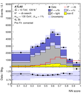
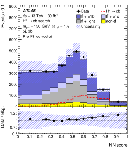
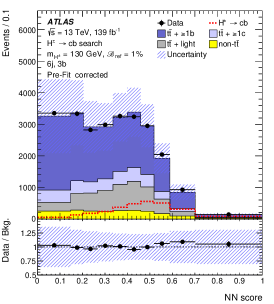
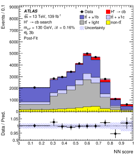
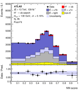
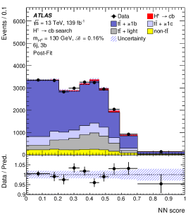
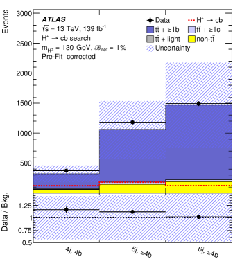
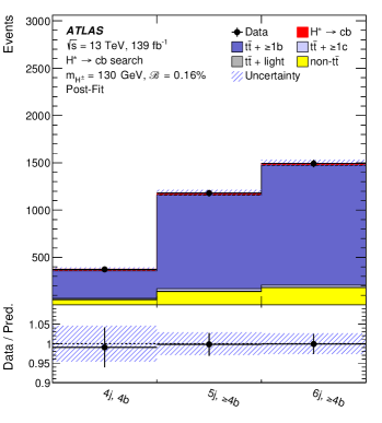
The best-fit $\mathscr{B}$ varies between 0.06% and 0.19% with an absolute uncertainty ranging from about 0.13% to 0.05% depending on $m_{{H}^{\pm}}$. The total uncertainties of the measured signal strengths are dominated by systematic uncertainties. The stability of the best-fit $\mathscr{B}$ values was confirmed by separately fitting events containing either one electron or a muon, by varying the nuisance parameters most correlated with $\mathscr{B}$, decorrelating $\mathscr{B}$ across jet multiplicities and by separately fitting data collected in different data-taking years.

Table 2: Pre-fit yields in each of the analysis regions considered. The $t\bar{t}$ background yields are corrected with the procedure described in Section 5.2. The contribution from $t\bar{t}$ production with rare $W\rightarrow cb$ decays is included in $t\bar{t}$+light. The small contributions from $t\bar{t}V$, $t\bar{t}H$, single-top-quark, $W/Z$+jets, diboson, $tHq$ and $tZq$ backgrounds are combined into a single background source referred to as “non-$t\bar{t}$”. The $H^{\pm}$ signal yields for $m_{{H}^{\pm}}=70$ GeV and $m_{{H}^{\pm}}=130$ GeV are normalised to $\mathscr{B}_{\mathrm{ref}}=1\%$. The quoted uncertainties are the sum in quadrature of statistical and systematic uncertainties of the yields, computed taking into account correlations among processes resulting from the data-based $t\bar{t}$ correction procedure (see Sect. 5.2).

	4j, 2b + 1bl	5j, 2b + 1bl	6j, 2b + 1bl
$H^{\pm}\rightarrow cb$, $m_{{H}^{\pm}}=70$ GeV	$$3\,772$\pm\leavevmode\nobreak\ \leavevmode\nobreak\ \,$269$$	$$2\,703$\pm\leavevmode\nobreak\ \leavevmode\nobreak\ \,$220$$	$$1\,272$\pm\leavevmode\nobreak\ \leavevmode\nobreak\ \,$187$$
$H^{\pm}\rightarrow cb$, $m_{{H}^{\pm}}=130$ GeV	$$3\,547$\pm\leavevmode\nobreak\ \leavevmode\nobreak\ \,$265$$	$$2\,619$\pm\leavevmode\nobreak\ \leavevmode\nobreak\ \,$245$$	$$1\,311$\pm\leavevmode\nobreak\ \leavevmode\nobreak\ \,$181$$
$t\bar{t}$+$\geq$1b	$$4\,877$\pm$2\,680$$	$$7\,412$\pm$3\,817$$	$$6\,019$\pm$3\,185$$
$t\bar{t}$+$\geq$1c	$$5\,178$\pm$2\,646$$	$$6\,576$\pm$3\,409$$	$$4\,747$\pm$2\,549$$
$t\bar{t}$+light	$$27\,912$\pm$3\,596$$	$$19\,697$\pm$3\,676$$	$$9\,103$\pm$2\,375$$
Non-$t\bar{t}$ backgrounds	$$2\,890$\pm\leavevmode\nobreak\ \leavevmode\nobreak\ \,$609$$	$$2\,298$\pm\leavevmode\nobreak\ \leavevmode\nobreak\ \,$464$$	$$1\,366$\pm\leavevmode\nobreak\ \leavevmode\nobreak\ \,$305$$
Total background (Pre-Fit corrected)	$$40\,858$\pm$3\,333$$	$$35\,983$\pm$3\,486$$	$$21\,234$\pm$2\,994$$
Data	40 889	35 995	21 210
	4j, 3b	5j, 3b	6j, 3b
$H^{\pm}\rightarrow cb$, $m_{{H}^{\pm}}=70$ GeV	$$6\,600$\pm\leavevmode\nobreak\ \leavevmode\nobreak\ \,$600$$	$$4\,652$\pm\leavevmode\nobreak\ \leavevmode\nobreak\ \,$401$$	$$2\,222$\pm\leavevmode\nobreak\ \leavevmode\nobreak\ \,$283$$
$H^{\pm}\rightarrow cb$, $m_{{H}^{\pm}}=130$ GeV	$$5\,837$\pm\leavevmode\nobreak\ \leavevmode\nobreak\ \,$563$$	$$4\,504$\pm\leavevmode\nobreak\ \leavevmode\nobreak\ \,$408$$	$$2\,220$\pm\leavevmode\nobreak\ \leavevmode\nobreak\ \,$286$$
$t\bar{t}$+$\geq$1b	$$8\,839$\pm$4\,837$$	$$13\,888$\pm$7\,172$$	$$11\,543$\pm$6\,132$$
$t\bar{t}$+$\geq$1c	$$2\,508$\pm$1\,291$$	$$3\,269$\pm$1\,715$$	$$2\,365$\pm$1\,283$$
$t\bar{t}$+light	$$11\,130$\pm$1\,602$$	$$7\,771$\pm$1\,509$$	$$3\,590$\pm\leavevmode\nobreak\ \leavevmode\nobreak\ \,$943$$
Non-$t\bar{t}$ backgrounds	$$2\,453$\pm\leavevmode\nobreak\ \leavevmode\nobreak\ \,$467$$	$$2\,383$\pm\leavevmode\nobreak\ \leavevmode\nobreak\ \,$418$$	$$1\,588$\pm\leavevmode\nobreak\ \leavevmode\nobreak\ \,$308$$
Total background (Pre-Fit corrected)	$$24\,931$\pm$4\,459$$	$$27\,310$\pm$6\,162$$	$$19\,087$\pm$5\,419$$
Data	26 614	28 394	19 302
	4j, 4b	5j, $\geq$4b	6j, $\geq$4b
$H^{\pm}\rightarrow cb$, $m_{{H}^{\pm}}=70$ GeV	$$138$\pm\leavevmode\nobreak\ \leavevmode\nobreak\ $39$$	$$168$\pm\leavevmode\nobreak\ \leavevmode\nobreak\ $43$$	$$119$\pm\leavevmode\nobreak\ \leavevmode\nobreak\ $56$$
$H^{\pm}\rightarrow cb$, $m_{{H}^{\pm}}=130$ GeV	$$123$\pm\leavevmode\nobreak\ \leavevmode\nobreak\ $35$$	$$181$\pm\leavevmode\nobreak\ \leavevmode\nobreak\ $47$$	$$124$\pm\leavevmode\nobreak\ \leavevmode\nobreak\ $59$$
$t\bar{t}$+$\geq$1b	$$248$\pm$139$$	$$871$\pm$486$$	$$1\,246$\pm$710$$
$t\bar{t}$+$\geq$1c	$$10$\pm\leavevmode\nobreak\ \leavevmode\nobreak\ \leavevmode\nobreak\ \leavevmode\nobreak\ $7$$	$$26$\pm\leavevmode\nobreak\ \leavevmode\nobreak\ $14$$	$$25$\pm\leavevmode\nobreak\ \leavevmode\nobreak\ $14$$
$t\bar{t}$+light	$$5$\pm\leavevmode\nobreak\ \leavevmode\nobreak\ \leavevmode\nobreak\ \leavevmode\nobreak\ $3$$	$$8$\pm\leavevmode\nobreak\ \leavevmode\nobreak\ \leavevmode\nobreak\ \leavevmode\nobreak\ $6$$	$$6$\leavevmode\nobreak\ \leavevmode\nobreak\ \leavevmode\nobreak\ \leavevmode\nobreak\ \pm$5$$
Non-$t\bar{t}$ backgrounds	$$57$\pm\leavevmode\nobreak\ \leavevmode\nobreak\ $15$$	$$146$\pm\leavevmode\nobreak\ \leavevmode\nobreak\ $26$$	$\leavevmode\nobreak\ \leavevmode\nobreak\ \,$191$\pm\leavevmode\nobreak\ \leavevmode\nobreak\ $41$$
Total background (Pre-Fit corrected)	$$322$\pm$142$$	$$1\,052$\pm$484$$	$$1\,468$\pm$708$$
Data	374	1 179	1 492

Table 3: Post-fit yields in each of the fit regions considered; the analysis regions used to derive the data-based $t\bar{t}$ corrections are not used in the fit, so their yields are not displayed. The contribution from $t\bar{t}$ production with rare $W\rightarrow cb$ decays is included in $t\bar{t}$+light. The total prediction is shown after the fit to data under the signal-plus-background hypothesis assuming $H^{\pm}$ signal with $m_{{H}^{\pm}}=130$ GeV. The predicted yields for the $H^{\pm}$ signal with $m_{{H}^{\pm}}=70$ GeV are also shown for reference. The best fit-values of $\mathscr{B}$ for $H^{\pm}$ signal with $m_{{H}^{\pm}}=130$ GeV and $m_{{H}^{\pm}}=70$ GeV are 0.16% and 0.07% respectively. The small contributions from $t\bar{t}V$, $t\bar{t}H$, single-top-quark, $W/Z$+jets, diboson, $tHq$ and $tZq$ backgrounds are combined into a single background source referred to as “non-$t\bar{t}$”. The quoted uncertainties are the sum in quadrature of statistical and systematic uncertainties of the yields, computed taking into account correlations among nuisance parameters and among processes.

	4j, 3b	5j, 3b	6j, 3b
$H^{\pm}\rightarrow cb$, $m_{{H}^{\pm}}=70$ GeV	$$450$\pm\leavevmode\nobreak\ \leavevmode\nobreak\ \,$382$$	$$325$\pm\leavevmode\nobreak\ \leavevmode\nobreak\ \,$275$$	$$152$\pm$130$$
$H^{\pm}\rightarrow cb$, $m_{{H}^{\pm}}=130$ GeV	$$923$\pm\leavevmode\nobreak\ \leavevmode\nobreak\ \,$345$$	$$682$\pm\leavevmode\nobreak\ \leavevmode\nobreak\ \,$255$$	$$333$\pm$127$$
$t\bar{t}$+$\geq$1b	$$10\,678$\pm\leavevmode\nobreak\ \leavevmode\nobreak\ \,$727$$	$$15\,745$\pm\leavevmode\nobreak\ \leavevmode\nobreak\ \,$908$$	$$12\,344$\pm$655$$
$t\bar{t}$+$\geq$1c	$$2\,758$\pm$1\,113$$	$$3\,397$\pm$1\,361$$	$\leavevmode\nobreak\ \leavevmode\nobreak\ $2\,353$\pm$946$$
$t\bar{t}$+light	$$9\,969$\pm\leavevmode\nobreak\ \leavevmode\nobreak\ \,$694$$	$$6\,378$\pm\leavevmode\nobreak\ \leavevmode\nobreak\ \,$699$$	$\leavevmode\nobreak\ \leavevmode\nobreak\ $2\,813$\pm$411$$
Non-$t\bar{t}$ backgrounds	$$2\,287$\pm\leavevmode\nobreak\ \leavevmode\nobreak\ \,$413$$	$$2\,195$\pm\leavevmode\nobreak\ \leavevmode\nobreak\ \,$388$$	$$1\,459$\pm$285$$
Total prediction	$$26\,615$\pm\leavevmode\nobreak\ \leavevmode\nobreak\ \,$249$$	$$28\,397$\pm\leavevmode\nobreak\ \leavevmode\nobreak\ \,$313$$	$$19\,302$\pm$246$$
Data	26 614	28 394	19 302
	4j, 4b	5j, $\geq$4b	6j, $\geq$4b
$H^{\pm}\rightarrow cb$, $m_{{H}^{\pm}}=70$ GeV	$$8$\pm\leavevmode\nobreak\ \leavevmode\nobreak\ $7$$	$$12$\pm$11$$	$$7$\pm\leavevmode\nobreak\ \leavevmode\nobreak\ $6$$
$H^{\pm}\rightarrow cb$, $m_{{H}^{\pm}}=130$ GeV	$$20$\pm\leavevmode\nobreak\ \leavevmode\nobreak\ $8$$	$$25$\pm$11$$	$$21$\pm$11$$
$t\bar{t}$+$\geq$1b	$$291$\pm$23$$	$\leavevmode\nobreak\ \leavevmode\nobreak\ \,$987$\pm$46$$	$$1\,266$\pm$57$$
$t\bar{t}$+$\geq$1c	$$11$\pm\leavevmode\nobreak\ \leavevmode\nobreak\ $7$$	$$26$\pm$11$$	$\leavevmode\nobreak\ \leavevmode\nobreak\ \leavevmode\nobreak\ \leavevmode\nobreak\ \,$24$\pm$11$$
$t\bar{t}$+light	$$3$\pm\leavevmode\nobreak\ \leavevmode\nobreak\ $2$$	$$4$\pm\leavevmode\nobreak\ \leavevmode\nobreak\ $4$$	$$4$\pm\leavevmode\nobreak\ \leavevmode\nobreak\ $3$$
Non-$t\bar{t}$ backgrounds	$$52$\pm$13$$	$\leavevmode\nobreak\ \leavevmode\nobreak\ \,$138$\pm$26$$	$\leavevmode\nobreak\ \leavevmode\nobreak\ \,$179$\pm$40$$
Total prediction	$$378$\pm$17$$	$$1\,182$\pm$34$$	$$1\,494$\pm$38$$
Data	374	1 179	1 492

Figure 8: The observed (solid) 95% CL upper limits on $\mathscr{B}=\mathscr{B}(t\rightarrow H^{\pm}b)\times\mathscr{B}(H^{\pm}\rightarrow cb)$ as a function of $m_{{H}^{\pm}}$ and the expectation (dashed) under the background-only hypothesis. The inner green and outer yellow shaded bands show the $\pm 1\sigma$ and $\pm 2\sigma$ uncertainties of the expected limits. The exclusion limits are presented for $m_{{H}^{\pm}}$ between 60 and 160 GeV with 10 GeV $m_{{H}^{\pm}}$ spacing and linear interpolation between adjacent mass points. Superimposed on the upper limits, the predictions from the 3HDM [21, 22] are shown, corresponding to three benchmark values for the parameters $X$, $Y$, and $Z$ described in the text.

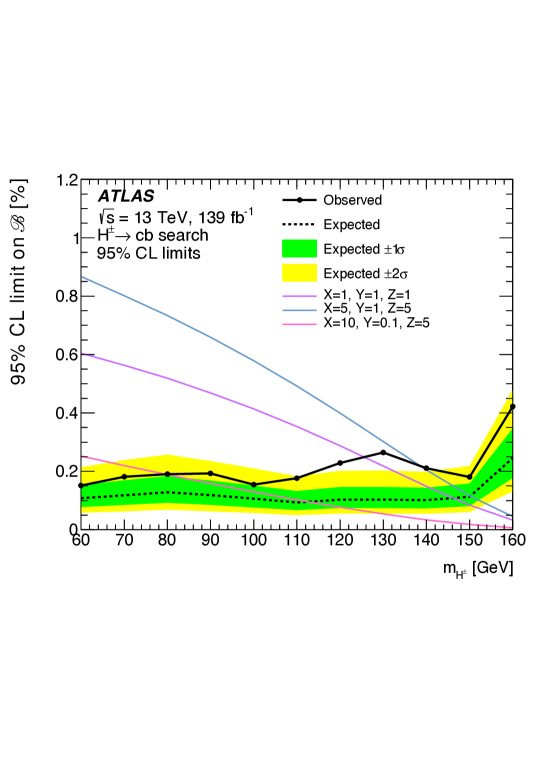
There is no significant excess of data events above the background expectation, and 95% CL limits are set on the product of branching fractions $\mathscr{B}$. Figure 8 shows the observed (expected) 95% CL upper limits on the branching fraction $\mathscr{B}$ as a function of $m_{{H}^{\pm}}$; they range from 0.15% (0.09%) up to 0.42% (0.25%) depending on $m_{{H}^{\pm}}$. The acceptance loss for the $b$-jet produced from the decay $t\rightarrow H^{\pm}b$ increases for $m_{{H}^{\pm}}$ close to the top-quark mass, resulting in weaker exclusion limits. Superimposed on the upper limits, the predictions from the 3HDM [21, 22] are shown, corresponding to three benchmark values for the parameters $X$, $Y$, and $Z$, which are functions of the Higgs-doublet vacuum expectation values and the mixing angle between the charged Higgs bosons.

The observed exclusion limits are consistently weaker than the expectation. The largest excess in data has a local significance of about $3\sigma$ for $m_{{H}^{\pm}}=130$ GeV. The corresponding best-fit $\mathscr{B}$ is measured to be $(0.16\pm 0.06)$%.

Pseudo-experiments from simulated events are generated to estimate the global significance of this excess. In the first step, the correlation across all bins of the NN score distributions for all $m_{{H}^{\pm}}$ hypotheses is estimated using the MC samples. Next, the pseudo-data are generated by fluctuating all NN score distribution bins corresponding to the pre-fit background expectation within their statistical uncertainty while preserving the correlations across all $m_{{H}^{\pm}}$ values. Each generated pseudo-experiment is analysed with the test statistic described in Section 7 built for each of the considered $m_{{H}^{\pm}}$ hypothesis. The global $p$-value is then calculated as the fraction of times the maximum local significance in each pseudo-experiment exceeds the maximum local significance observed in data. This procedure leads to a global significance of $(2.46\pm 0.05)\sigma$ in the considered $m_{{H}^{\pm}}$ range, with the uncertainty originating from the pseudo-experiments’ sample size.

Studies using pseudo-data, defined as the sum of all predicted post-fit backgrounds plus an injected signal of variable strength, were performed to validate the behaviour of the exclusion limits as a function of $m_{{H}^{\pm}}$. It was concluded that a broad excess in the considered $m_{{H}^{\pm}}$ range is consistent with the $m_{{H}^{\pm}}$ resolution, which is significantly worse than the expected dijet mass resolution ($\sim$$15\%$) due to the ambiguity in choosing the correct $b$-jet to pair with the fourth jet to reconstruct the $m_{{H}^{\pm}}$ mass.

8 Conclusion

A search for the $H^{\pm}\rightarrow cb$ decay mode in top-quark decays is presented. The search uses a dataset of $pp$ collisions collected at a centre-of-mass energy $\sqrt{s}=13\;\text{TeV}$ between 2015 and 2018 with the ATLAS detector at CERN’s Large Hadron Collider, amounting to an integrated luminosity of 139 fb^-1. The analysis focuses on a data sample enriched in top-quark pair production, where one top quark decays into a leptonically decaying $W$ boson and a bottom quark, and the other top quark may decay into a $H^{\pm}$ boson and a bottom quark. The search exploits the high multiplicity of $b$-jets, as expected from signal events, and deploys a neural network classifier that uses the kinematic differences between the signal and the background. In the absence of a significant excess of data events above the background expectation, model-independent exclusion limits at 95% confidence level on the product of branching fractions $\mathscr{B}=\mathscr{B}(t\rightarrow H^{\pm}b)\,\times\mathscr{B}(H^{\pm}\rightarrow cb)$ are reported as a function of $m_{{H}^{\pm}}$. The observed (expected) limits vary between 0.15% (0.09%) and 0.42% (0.25%) for $m_{{H}^{\pm}}$ between 60 and 160 GeV. The largest excess in data has a significance of about $3\sigma$ for $m_{{H}^{\pm}}=130$ GeV. In the considered $m_{{H}^{\pm}}$ range the global significance is estimated to be about 2.5$\sigma$.

Thanks to a much larger dataset and improved analysis techniques, this search has an expected sensitivity to $H^{\pm}\rightarrow cb$ in top-quark decays that is a factor of five higher than achieved in a previous search by the CMS Collaboration and explores an extended $m_{{H}^{\pm}}$ range.

References

- [1] ATLAS Collaboration “Observation of a new particle in the search for the Standard Model Higgs boson with the ATLAS detector at the LHC” In Phys. Lett. B 716, 2012, pp. 1 DOI: 10.1016/j.physletb.2012.08.020
- [2] CMS Collaboration “Observation of a new boson at a mass of 125 GeV with the CMS experiment at the LHC” In Phys. Lett. B 716, 2012, pp. 30 DOI: 10.1016/j.physletb.2012.08.021
- [3] ATLAS Collaboration “A detailed map of Higgs boson interactions by the ATLAS experiment ten years after the discovery” In Nature 607.7917, 2022, pp. 52–59 DOI: 10.1038/s41586-022-04893-w
- [4] CMS Collaboration “A portrait of the Higgs boson by the CMS experiment ten years after the discovery” In Nature 607.7917, 2022, pp. 60–68 DOI: 10.1038/s41586-022-04892-x
- [5] F. Englert and R. Brout “Broken Symmetry and the Mass of Gauge Vector Mesons” In Phys. Rev. Lett. 13, 1964, pp. 321–323 DOI: 10.1103/PhysRevLett.13.321
- [6] Peter W. Higgs “Broken symmetries, massless particles and gauge fields” In Phys. Lett. 12, 1964, pp. 132–133 DOI: 10.1016/0031-9163(64)91136-9
- [7] Peter W. Higgs “Broken Symmetries and the Masses of Gauge Bosons” In Phys. Rev. Lett. 13, 1964, pp. 508–509 DOI: 10.1103/PhysRevLett.13.508
- [8] G.. Guralnik, C.. Hagen and T… Kibble “Global Conservation Laws and Massless Particles” In Phys. Rev. Lett. 13, 1964, pp. 585–587 DOI: 10.1103/PhysRevLett.13.585
- [9] Peter W. Higgs “Spontaneous Symmetry Breakdown without Massless Bosons” In Phys. Rev. 145, 1966, pp. 1156–1163 DOI: 10.1103/PhysRev.145.1156
- [10] T… Kibble “Symmetry Breaking in Non-Abelian Gauge Theories” In Phys. Rev. 155, 1967, pp. 1554–1561 DOI: 10.1103/PhysRev.155.1554
- [11] G.. Branco et al. “Theory and phenomenology of two-Higgs-doublet models” In Phys. Rept. 516, 2012, pp. 1–102 DOI: 10.1016/j.physrep.2012.02.002
- [12] Sheldon L. Glashow and Steven Weinberg “Natural conservation laws for neutral currents” In Phys. Rev. D 15, 1977, pp. 1958 DOI: 10.1103/PhysRevD.15.1958
- [13] Frank E. Paige, Emmanuel A. Paschos and T.. Trueman “Constraints on gauge theories with diagonal neutral currents” In Phys. Rev. D 15, 1977, pp. 3416 DOI: 10.1103/PhysRevD.15.3416
- [14] Pierre Fayet “Supersymmetry and weak, electromagnetic and strong Interactions” In Phys. Lett. B 64, 1976, pp. 159 DOI: 10.1016/0370-2693(76)90319-1
- [15] Pierre Fayet “Spontaneously broken supersymmetric theories of weak, electromagnetic and strong Interactions” In Phys. Lett. B 69, 1977, pp. 489 DOI: 10.1016/0370-2693(77)90852-8
- [16] Jihn E. Kim “Light pseudoscalars, particle physics and cosmology” In Phys. Rept. 150, 1987, pp. 1–177 DOI: 10.1016/0370-1573(87)90017-2
- [17] A.. Akeroyd “Prospects for charged Higgs searches at the LHC” In Eur. Phys. J. C 77.5, 2017, pp. 276 DOI: 10.1140/epjc/s10052-017-4829-2
- [18] Felix Kling, Shufang Su and Wei Su “2HDM neutral scalars under the LHC” In JHEP 06, 2020, pp. 163 DOI: 10.1007/JHEP06(2020)163
- [19] ATLAS Collaboration “Combined measurements of Higgs boson production and decay using up to of proton–proton collision data at collected with the ATLAS experiment” In Phys. Rev. D 101, 2020, pp. 012002 DOI: 10.1103/PhysRevD.101.012002
- [20] CMS Collaboration “Combined measurements of Higgs boson couplings in proton–proton collisions at ” In Eur. Phys. J. C 79, 2019, pp. 421 DOI: 10.1140/epjc/s10052-019-6909-y
- [21] A.. Akeroyd, Stefano Moretti, Kei Yagyu and Emine Yildirim “Light charged Higgs boson scenario in 3-Higgs doublet models” In Int. J. Mod. Phys. A 32.23n24, 2017, pp. 1750145 DOI: 10.1142/S0217751X17501457
- [22] A.. Akeroyd, Stefano Moretti and Muyuan Song “Light charged Higgs boson with dominant decay to quarks and its search at the LHC and future colliders” In Phys. Rev. D 98.11, 2018, pp. 115024 DOI: 10.1103/PhysRevD.98.115024
- [23] CMS Collaboration “Search for a charged Higgs boson decaying to charm and bottom quarks in proton–proton collisions at ” In JHEP 11, 2018, pp. 115 DOI: 10.1007/JHEP11(2018)115
- [24] ATLAS Collaboration “Search for a light charged Higgs boson in the decay channel in events using collisions at with the ATLAS detector” In Eur. Phys. J. C 73, 2013, pp. 2465 DOI: 10.1140/epjc/s10052-013-2465-z
- [25] CMS Collaboration “Search for a light charged Higgs boson decaying to in collisions at ” In JHEP 12, 2015, pp. 178 DOI: 10.1007/JHEP12(2015)178
- [26] ATLAS Collaboration “The ATLAS Experiment at the CERN Large Hadron Collider” In JINST 3, 2008, pp. S08003 DOI: 10.1088/1748-0221/3/08/S08003
- [27] ATLAS Collaboration “The ATLAS Collaboration Software and Firmware”, ATL-SOFT-PUB-2021-001, 2021 URL: https://cds.cern.ch/record/2767187
- [28] ATLAS Collaboration “ATLAS data quality operations and performance for 2015–2018 data-taking” In JINST 15.04, 2020, pp. P04003 DOI: 10.1088/1748-0221/15/04/P04003
- [29] ATLAS Collaboration “Luminosity determination in collisions at using the ATLAS detector at the LHC”, ATLAS-CONF-2019-021, 2019 URL: https://cds.cern.ch/record/2677054
- [30] G. Avoni “The new LUCID-2 detector for luminosity measurement and monitoring in ATLAS” In JINST 13.07, 2018, pp. P07017 DOI: 10.1088/1748-0221/13/07/P07017
- [31] ATLAS Collaboration “Performance of the ATLAS muon triggers in Run 2” In JINST 15.09, 2020, pp. P09015 DOI: 10.1088/1748-0221/15/09/p09015
- [32] ATLAS Collaboration “Performance of electron and photon triggers in ATLAS during LHC Run 2” In Eur. Phys. J. C 80.1, 2020, pp. 47 DOI: 10.1140/epjc/s10052-019-7500-2
- [33] ATLAS Collaboration “Operation of the ATLAS trigger system in Run 2” In JINST 15.10, 2020, pp. P10004 DOI: 10.1088/1748-0221/15/10/P10004
- [34] ATLAS Collaboration “The ATLAS inner detector trigger performance in pp collisions at 13 TeV during LHC Run 2” In Eur. Phys. J. C 82.3, 2022, pp. 206 DOI: 10.1140/epjc/s10052-021-09920-0
- [35] ATLAS Collaboration “Electron and photon performance measurements with the ATLAS detector using the 2015–2017 LHC proton-proton collision data” In JINST 14.12, 2019, pp. P12006 DOI: 10.1088/1748-0221/14/12/P12006
- [36] ATLAS Collaboration “Muon reconstruction and identification efficiency in ATLAS using the full Run 2 collision data set at TeV” In Eur. Phys. J. C 81, 2021, pp. 578 DOI: 10.1140/epjc/s10052-021-09233-2
- [37] ATLAS Collaboration “Topological cell clustering in the ATLAS calorimeters and its performance in LHC Run 1” In Eur. Phys. J. C 77, 2017, pp. 490 DOI: 10.1140/epjc/s10052-017-5004-5
- [38] ATLAS Collaboration “Jet reconstruction and performance using particle flow with the ATLAS Detector” In Eur. Phys. J. C 77.7, 2017, pp. 466 DOI: 10.1140/epjc/s10052-017-5031-2
- [39] Matteo Cacciari, Gavin P. Salam and Gregory Soyez “FastJet user manual” In Eur. Phys. J. C 72, 2012, pp. 1896 DOI: 10.1140/epjc/s10052-012-1896-2
- [40] Matteo Cacciari, Gavin P. Salam and Gregory Soyez “The anti- jet clustering algorithm” In JHEP 04, 2008, pp. 063 DOI: 10.1088/1126-6708/2008/04/063
- [41] ATLAS Collaboration “Jet energy scale and resolution measured in proton–proton collisions at TeV with the ATLAS detector” In Eur. Phys. J. C 81.8, 2021, pp. 689 DOI: 10.1140/epjc/s10052-021-09402-3
- [42] ATLAS Collaboration “Performance of pile-up mitigation techniques for jets in collisions at TeV using the ATLAS detector” In Eur. Phys. J. C 76.11, 2016, pp. 581 DOI: 10.1140/epjc/s10052-016-4395-z
- [43] ATLAS Collaboration “ATLAS flavour-tagging algorithms for the LHC Run 2 collision dataset”, 2022 arXiv:2211.16345 [physics.data-an]
- [44] ATLAS Collaboration “Performance of missing transverse momentum reconstruction with the ATLAS detector using proton-proton collisions at = 13 TeV” In Eur. Phys. J. C 78.11, 2018, pp. 903 DOI: 10.1140/epjc/s10052-018-6288-9
- [45] ATLAS Collaboration “Observation of the associated production of a top quark and a boson in collisions at TeV with the ATLAS detector” In JHEP 07, 2020, pp. 124 DOI: 10.1007/JHEP07(2020)124
- [46] ATLAS Collaboration “Search for charged Higgs bosons decaying into a top quark and a bottom quark at = 13 TeV with the ATLAS detector” In JHEP 06, 2021, pp. 145 DOI: 10.1007/JHEP06(2021)145
- [47] NNPDF Collaboration and Richard D. Ball “Parton distributions with LHC data” In Nucl. Phys. B 867, 2013, pp. 244 DOI: 10.1016/j.nuclphysb.2012.10.003
- [48] T. Sjöstrand, S. Mrenna and P. Skands “A brief introduction to PYTHIA 8.1” In Comput. Phys. Commun. 178, 2008, pp. 852–867 DOI: 10.1016/j.cpc.2008.01.036
- [49] M. Bähr “Herwig++ physics and manual” In Eur. Phys. J. C 58, 2008, pp. 639 DOI: 10.1140/epjc/s10052-008-0798-9
- [50] Johannes Bellm “Herwig 7.0/Herwig++ 3.0 release note” In Eur. Phys. J. C 76.4, 2016, pp. 196 DOI: 10.1140/epjc/s10052-016-4018-8
- [51] D.. Lange “The EvtGen particle decay simulation package” In Proceedings, 7th International Conference on B physics at hadron machines (BEAUTY 2000) 462, 2001, pp. 152 DOI: 10.1016/S0168-9002(01)00089-4
- [52] Torbjörn Sjöstrand et al. “An introduction to PYTHIA 8.2” In Comput. Phys. Commun. 191, 2015, pp. 159 DOI: 10.1016/j.cpc.2015.01.024
- [53] ATLAS Collaboration “ATLAS Pythia 8 tunes to data”, ATL-PHYS-PUB-2014-021, 2014 URL: https://cds.cern.ch/record/1966419
- [54] L.. Harland-Lang, A.. Martin, P. Motylinski and R.. Thorne “Parton distributions in the LHC era: MMHT 2014 PDFs” In Eur. Phys. J. C 75.5, 2015, pp. 204 DOI: 10.1140/epjc/s10052-015-3397-6
- [55] The NNPDF Collaboration and Richard D. Ball “Parton distributions for the LHC run II” In JHEP 04, 2015, pp. 040 DOI: 10.1007/JHEP04(2015)040
- [56] ATLAS Collaboration “The Pythia 8 A3 tune description of ATLAS minimum bias and inelastic measurements incorporating the Donnachie–Landshoff diffractive model”, ATL-PHYS-PUB-2016-017, 2016 URL: https://cds.cern.ch/record/2206965
- [57] ATLAS Collaboration “The ATLAS simulation infrastructure” In Eur. Phys. J. C 70, 2010, pp. 823 DOI: 10.1140/epjc/s10052-010-1429-9
- [58] S. Agostinelli “Geant4 – a simulation toolkit” In Nucl. Instrum. Meth. A 506, 2003, pp. 250 DOI: 10.1016/S0168-9002(03)01368-8
- [59] ATLAS Collaboration “The simulation principle and performance of the ATLAS fast calorimeter simulation FastCaloSim” In ATL-PHYS-PUB-2010-013, 2010 URL: https://cds.cern.ch/record/1300517
- [60] Stefano Frixione, Giovanni Ridolfi and Paolo Nason “A positive-weight next-to-leading-order Monte Carlo for heavy flavour hadroproduction” In JHEP 09, 2007, pp. 126 DOI: 10.1088/1126-6708/2007/09/126
- [61] Paolo Nason “A new method for combining NLO QCD with shower Monte Carlo algorithms” In JHEP 11, 2004, pp. 040 DOI: 10.1088/1126-6708/2004/11/040
- [62] Stefano Frixione, Paolo Nason and Carlo Oleari “Matching NLO QCD computations with parton shower simulations: the POWHEG method” In JHEP 11, 2007, pp. 070 DOI: 10.1088/1126-6708/2007/11/070
- [63] Simone Alioli, Paolo Nason, Carlo Oleari and Emanuele Re “A general framework for implementing NLO calculations in shower Monte Carlo programs: the POWHEG BOX” In JHEP 06, 2010, pp. 043 DOI: 10.1007/JHEP06(2010)043
- [64] ATLAS Collaboration “Studies on top-quark Monte Carlo modelling for Top2016”, ATL-PHYS-PUB-2016-020, 2016 URL: https://cds.cern.ch/record/2216168
- [65] Fabio Maltoni, Giovanni Ridolfi and Maria Ubiali “b-initiated processes at the LHC: a reappraisal” In JHEP 07, 2012, pp. 022 DOI: 10.1007/JHEP07(2012)022
- [66] ATLAS Collaboration “Search for top-quark decays with 36 fb-1 of collision data at TeV with the ATLAS detector” In JHEP 05, 2019, pp. 123 DOI: 10.1007/JHEP05(2019)123
- [67] Tomáš Ježo, Jonas M. Lindert, Niccolo Moretti and Stefano Pozzorini “New NLOPS predictions for -jet production at the LHC” In Eur. Phys. J. C 78.6, 2018, pp. 502 DOI: 10.1140/epjc/s10052-018-5956-0
- [68] Federico Buccioni et al. “OpenLoops 2” In Eur. Phys. J. C 79.10, 2019, pp. 866 DOI: 10.1140/epjc/s10052-019-7306-2
- [69] Fabio Cascioli, Philipp Maierhöfer and Stefano Pozzorini “Scattering Amplitudes with Open Loops” In Phys. Rev. Lett. 108, 2012, pp. 111601 DOI: 10.1103/PhysRevLett.108.111601
- [70] Ansgar Denner, Stefan Dittmaier and Lars Hofer “Collier: A fortran-based complex one-loop library in extended regularizations” In Comput. Phys. Commun. 212, 2017, pp. 220–238 DOI: 10.1016/j.cpc.2016.10.013
- [71] Tomas Ježo “Powheg-Box-Res ttbb source code”, 2019 URL: https://gitlab.cern.ch/tjezo/powheg-box-res_ttbb/
- [72] Stefano Frixione, Eric Laenen, Patrick Motylinski and Bryan R. Webber “Angular correlations of lepton pairs from vector boson and top quark decays in Monte Carlo simulations” In JHEP 04, 2007, pp. 081 DOI: 10.1088/1126-6708/2007/04/081
- [73] Pierre Artoisenet, Rikkert Frederix, Olivier Mattelaer and Robbert Rietkerk “Automatic spin-entangled decays of heavy resonances in Monte Carlo simulations” In JHEP 03, 2013, pp. 015 DOI: 10.1007/JHEP03(2013)015
- [74] M. Beneke, P. Falgari, S. Klein and C. Schwinn “Hadronic top-quark pair production with NNLL threshold resummation” In Nucl. Phys. B 855, 2012, pp. 695–741 DOI: 10.1016/j.nuclphysb.2011.10.021
- [75] Matteo Cacciari et al. “Top-pair production at hadron colliders with next-to-next-to-leading logarithmic soft-gluon resummation” In Phys. Lett. B 710, 2012, pp. 612–622 DOI: 10.1016/j.physletb.2012.03.013
- [76] Peter Bärnreuther, Michal Czakon and Alexander Mitov “Percent-Level-Precision Physics at the Tevatron: Next-to-Next-to-Leading Order QCD Corrections to ” In Phys. Rev. Lett. 109, 2012, pp. 132001 DOI: 10.1103/PhysRevLett.109.132001
- [77] Michal Czakon and Alexander Mitov “NNLO corrections to top-pair production at hadron colliders: the all-fermionic scattering channels” In JHEP 12, 2012, pp. 054 DOI: 10.1007/JHEP12(2012)054
- [78] Michal Czakon and Alexander Mitov “NNLO corrections to top pair production at hadron colliders: the quark-gluon reaction” In JHEP 01, 2013, pp. 080 DOI: 10.1007/JHEP01(2013)080
- [79] Michal Czakon, Paul Fiedler and Alexander Mitov “Total Top-Quark Pair-Production Cross Section at Hadron Colliders Through ” In Phys. Rev. Lett. 110, 2013, pp. 252004 DOI: 10.1103/PhysRevLett.110.252004
- [80] Michal Czakon and Alexander Mitov “Top++: A program for the calculation of the top-pair cross-section at hadron colliders” In Comput. Phys. Commun. 185, 2014, pp. 2930 DOI: 10.1016/j.cpc.2014.06.021
- [81] Stefano Frixione et al. “Single-top hadroproduction in association with a boson” In JHEP 07, 2008, pp. 029 DOI: 10.1088/1126-6708/2008/07/029
- [82] Emanuele Re “Single-top -channel production matched with parton showers using the POWHEG method” In Eur. Phys. J. C 71, 2011, pp. 1547 DOI: 10.1140/epjc/s10052-011-1547-z
- [83] Nikolaos Kidonakis “Two-loop soft anomalous dimensions for single top quark associated production with a or ” In Phys. Rev. D 82, 2010, pp. 054018 DOI: 10.1103/PhysRevD.82.054018
- [84] Nikolaos Kidonakis “Top Quark Production” In Proceedings, Helmholtz International Summer School on Physics of Heavy Quarks and Hadrons (HQ 2013), pp. 139–168 DOI: 10.3204/DESY-PROC-2013-03/Kidonakis
- [85] M. Aliev et al. “HATHOR – HAdronic Top and Heavy quarks crOss section calculatoR” In Comput. Phys. Commun. 182, 2011, pp. 1034–1046 DOI: 10.1016/j.cpc.2010.12.040
- [86] P. Kant et al. “HatHor for single top-quark production: Updated predictions and uncertainty estimates for single top-quark production in hadronic collisions” In Comput. Phys. Commun. 191, 2015, pp. 74–89 DOI: 10.1016/j.cpc.2015.02.001
- [87] Enrico Bothmann “Event generation with Sherpa 2.2” In SciPost Phys. 7.3, 2019, pp. 034 DOI: 10.21468/SciPostPhys.7.3.034
- [88] Tanju Gleisberg and Stefan Höche “Comix, a new matrix element generator” In JHEP 12, 2008, pp. 039 DOI: 10.1088/1126-6708/2008/12/039
- [89] Steffen Schumann and Frank Krauss “A parton shower algorithm based on Catani–Seymour dipole factorisation” In JHEP 03, 2008, pp. 038 DOI: 10.1088/1126-6708/2008/03/038
- [90] Stefan Höche, Frank Krauss, Marek Schönherr and Frank Siegert “A critical appraisal of NLO+PS matching methods” In JHEP 09, 2012, pp. 049 DOI: 10.1007/JHEP09(2012)049
- [91] Stefan Höche, Frank Krauss, Marek Schönherr and Frank Siegert “QCD matrix elements + parton showers. The NLO case” In JHEP 04, 2013, pp. 027 DOI: 10.1007/JHEP04(2013)027
- [92] S. Catani, F. Krauss, B.. Webber and R. Kuhn “QCD Matrix Elements + Parton Showers” In JHEP 11, 2001, pp. 063 DOI: 10.1088/1126-6708/2001/11/063
- [93] Stefan Höche, Frank Krauss, Steffen Schumann and Frank Siegert “QCD matrix elements and truncated showers” In JHEP 05, 2009, pp. 053 DOI: 10.1088/1126-6708/2009/05/053
- [94] Charalampos Anastasiou, Lance Dixon, Kirill Melnikov and Frank Petriello “High-precision QCD at hadron colliders: Electroweak gauge boson rapidity distributions at next-to-next-to leading order” In Phys. Rev. D 69, 2004, pp. 094008 DOI: 10.1103/PhysRevD.69.094008
- [95] D. Florian “Handbook of LHC Higgs Cross Sections: 4. Deciphering the Nature of the Higgs Sector”, 2016 DOI: 10.23731/CYRM-2017-002
- [96] ATLAS Collaboration “Search for flavour-changing neutral current top quark decays in collisions at TeV with the ATLAS detector” In JHEP 12, 2015, pp. 061 DOI: 10.1007/JHEP12(2015)061
- [97] ATLAS Collaboration “Measurement of the tt production cross section in collisions at = 13 TeV with the ATLAS detector” In JHEP 11, 2021, pp. 118 DOI: 10.1007/JHEP11(2021)118
- [98] Sergey Ioffe and Christian Szegedy “Batch Normalization: Accelerating Deep Network Training by Reducing Internal Covariate Shift”, 2015 arXiv:1502.03167 [cs.LG]
- [99] Diederik P. Kingma and Jimmy Ba “Adam: A Method for Stochastic Optimization”, 2014 arXiv:1412.6980 [cs.LG]
- [100] R. Kohavi “A Study of Cross-Validation and Bootstrap for Accuracy Estimation and Model Selection” In Proceedings of the Fourteenth International Joint Conference on Artificial Intelligence 2.1, 1995, pp. 1137–1143 URL: https://dl.acm.org/doi/10.5555/1643031.1643047
- [101] N. Srivastava, G. Hinton, A. Krizhevsky, I. Sutskever and R. Salakhutdinov “Dropout: A Simple Way to Prevent Neural Networks from Overfitting” In J. Mach. Learn. Res. 15.1 JMLR.org, 2014, pp. 1929–1958 URL: https://dl.acm.org/doi/10.5555/2627435.2670313
- [102] Pierre Baldi et al. “Parameterized neural networks for high-energy physics” In Eur. Phys. J. C 76.5, 2016, pp. 235 DOI: 10.1140/epjc/s10052-016-4099-4
- [103] ATLAS Collaboration “Measurement of the Inelastic Proton-Proton Cross Section at TeV with the ATLAS Detector at the LHC” In Phys. Rev. Lett. 117.18, 2016, pp. 182002 DOI: 10.1103/PhysRevLett.117.182002
- [104] ATLAS Collaboration “Jet energy scale measurements and their systematic uncertainties in proton-proton collisions at TeV with the ATLAS detector” In Phys. Rev. D 96.7, 2017, pp. 072002 DOI: 10.1103/PhysRevD.96.072002
- [105] ATLAS Collaboration “ATLAS -jet identification performance and efficiency measurement with events in collisions at ” In Eur. Phys. J. C 79, 2019, pp. 970 DOI: 10.1140/epjc/s10052-019-7450-8
- [106] ATLAS Collaboration “Measurement of the -jet mistagging efficiency in events using collision data at collected with the ATLAS detector” In Eur. Phys. J. C 82, 2022, pp. 95 DOI: 10.1140/epjc/s10052-021-09843-w
- [107] ATLAS Collaboration “Calibration of the light-flavour jet mistagging efficiency of the -tagging algorithms with +jets events using 139 of ATLAS proton-proton collision data at TeV”, 2023 arXiv:2301.06319 [hep-ex]
- [108] ATLAS Collaboration “Studies on top-quark Monte Carlo modelling with Sherpa and MG5_aMC@NLO”, ATL-PHYS-PUB-2017-007, 2017 URL: https://cds.cern.ch/record/2261938
- [109] ATLAS Collaboration “Measurements of inclusive and differential fiducial cross-sections of production with additional heavy-flavour jets in proton-proton collisions at = 13 TeV with the ATLAS detector” In JHEP 04, 2019, pp. 046 DOI: 10.1007/JHEP04(2019)046
- [110] Particle Data Group and P.A. Zyla “Review of Particle Physics” In PTEP 2020.8, 2020, pp. 083C01 DOI: 10.1093/ptep/ptaa104
- [111] Nikolaos Kidonakis “Next-to-next-to-leading-order collinear and soft gluon corrections for t-channel single top quark production” In Phys. Rev. D 83, 2011, pp. 091503 DOI: 10.1103/PhysRevD.83.091503
- [112] Nikolaos Kidonakis “NNLL resummation for s-channel single top quark production” In Phys. Rev. D 81, 2010, pp. 054028 DOI: 10.1103/PhysRevD.81.054028
- [113] ATLAS Collaboration “Measurements of the production cross-section for a boson in association with -jets in proton-proton collisions at TeV with the ATLAS detector” In JHEP 07, 2020, pp. 044 DOI: 10.1007/JHEP07(2020)044
- [114] Johan Alwall “Comparative study of various algorithms for the merging of parton showers and matrix elements in hadronic collisions” In Eur. Phys. J. C 53, 2008, pp. 473–500 DOI: 10.1140/epjc/s10052-007-0490-5
- [115] John M. Campbell and R. Ellis “Update on vector boson pair production at hadron colliders” In Phys. Rev. D 60, 1999, pp. 113006 DOI: 10.1103/PhysRevD.60.113006
- [116] ATLAS Collaboration “Measurement of production cross sections and gauge boson polarisation in collisions at with the ATLAS detector” In Eur. Phys. J. C 79, 2019, pp. 535 DOI: 10.1140/epjc/s10052-019-7027-6
- [117] ATLAS Collaboration “Evidence for production in the multilepton final state in proton–proton collisions at TeV with the ATLAS detector” In Eur. Phys. J. C 80.11, 2020, pp. 1085 DOI: 10.1140/epjc/s10052-020-08509-3
- [118] ATLAS Collaboration “Measurement of the and cross sections in proton-proton collisions at TeV with the ATLAS detector” In Phys. Rev. D 99.7, 2019, pp. 072009 DOI: 10.1103/PhysRevD.99.072009
- [119] Wouter Verkerke and David Kirkby “The RooFit toolkit for data modeling”, 2003 arXiv:physics/0306116 [physics.data-an]
- [120] Wouter Verkerke and David Kirkby “RooFit Users Manual” URL: http://roofit.sourceforge.net
- [121] Glen Cowan, Kyle Cranmer, Eilam Gross and Ofer Vitells “Asymptotic formulae for likelihood-based tests of new physics” In Eur. Phys. J. C 71, 2011, pp. 1554 DOI: 10.1140/epjc/s10052-011-1554-0
- [122] Thomas Junk “Confidence level computation for combining searches with small statistics” In Nucl. Instrum. Meth. A 434, 1999, pp. 435 DOI: 10.1016/S0168-9002(99)00498-2
- [123] Alexander L. Read “Presentation of search results: the technique” In J. Phys. G 28, 2002, pp. 2693 DOI: 10.1088/0954-3899/28/10/313
- [124] ATLAS Collaboration “Measurements of inclusive and differential fiducial cross-sections of production with additional heavy-flavour jets in proton–proton collisions at with the ATLAS detector” In JHEP 04, 2019, pp. 046 DOI: 10.1007/JHEP04(2019)046
- [125] CMS Collaboration “Measurement of the cross section for production with additional jets and jets in collisions at ” In JHEP 07, 2020, pp. 125 DOI: 10.1007/JHEP07(2020)125
- [126] ATLAS Collaboration “ATLAS Computing Acknowledgements”, ATL-SOFT-PUB-2023-001, 2023 URL: https://cds.cern.ch/record/2869272
- [127] ATLAS Collaboration In Nature 612, 2022, pp. E24 DOI: 10.1038/s41586-022-05581-5
- [128] Fabio Maltoni, Giovanni Ridolfi and Maria Ubiali In JHEP 04, 2013, pp. 095 DOI: 10.1007/JHEP04(2013)095
- [129] Glen Cowan, Kyle Cranmer, Eilam Gross and Ofer Vitells In Eur. Phys. J. C 73, 2013, pp. 2501 DOI: 10.1140/epjc/s10052-013-2501-z