Cavity Moiré Materials: Controlling Magnetic Frustration with Quantum Light-Matter Interaction

Abstract

Cavity quantum electrodynamics (QED) studies the interaction between light and matter at the single quantum level and has played a central role in quantum science and technology. Combining the idea of cavity QED with moiré materials, we theoretically show that strong quantum light-matter interaction provides a way to control frustrated magnetism. Specifically, we develop a theory of moiré materials confined in a cavity consisting of thin polar van der Waals crystals. We show that nontrivial quantum geometry of moiré flat bands leads to electromagnetic vacuum dressing of electrons, which produces appreciable changes in single-electron energies and manifests itself as long-range electron hoppings. We apply our general formulation to a twisted transition metal dichalcogenide heterobilayer encapsulated by ultrathin hexagonal boron nitride layers and predict its phase diagram at different twist angles and light-matter coupling strengths. Our results indicate that the cavity confinement enables one to control magnetic frustration of moiré materials and might allow for realizing various exotic phases such as a quantum spin liquid.

Controlling exotic phases of matter has been an ongoing quest in condensed matter physics. Moiré materials are emerging platforms for studying strongly correlated phenomena, where a long-periodic moiré pattern is formed by two overlaid crystal layers with relative twists or different lattice constants. Such moiré superlattice induces reconstruction of electronic structures and realizes nearly flat bands at certain twist angles Lopes dos Santos et al. (2007); Bistritzer and MacDonald (2011); Carr et al. (2020). In flat-band systems, the kinetic energy of electrons is significantly suppressed and the effect of electron-electron interaction becomes important Koshino et al. (2018); Po et al. (2018). So far, a number of intriguing phenomena have been experimentally observed in twisted bilayer graphene Andrei and MacDonald (2020); Balents et al. (2020); Nuckolls et al. (2020), including metal-insulator transition Cao et al. (2018a); Burg et al. (2019); Chen et al. (2019a), flat-band superconductivity Cao et al. (2018b); Chen et al. (2019b); Codecido et al. (2019); Lu et al. (2019); Yankowitz et al. (2019), magnetism Sharpe et al. (2019); Chen et al. (2020); Liu et al. (2020); He et al. (2021), and fractional quantum Hall effect Dean et al. (2013); Hunt et al. (2013); Wang et al. (2015); Spanton et al. (2018). Owing to rapid advances in manipulation of van der Waals (vdW) heterostructures Liu et al. (2019); Vincent et al. (2021), moiré materials consisting of transition metal dichalcogenides (TMDs) have also been extensively investigated Kennes et al. (2021); Wu et al. (2018); Classen et al. (2019); Xian et al. (2019); Wu et al. (2019); Pan et al. (2020a, b); Angeli and MacDonald (2021); Hu and MacDonald (2021); Morales-Durán et al. (2021); Zang et al. (2021); Xian et al. (2021); Zang et al. (2022). In particular, the high tunability of TMDs enables one to study various correlated phases Jin et al. (2019); Ni et al. (2019); Regan et al. (2020); Shimazaki et al. (2020); Tang et al. (2020); Wang et al. (2020); Xu et al. (2020); Zhang et al. (2020a); Huang et al. (2021); Jin et al. (2021); Yasuda et al. (2021); Li et al. (2021) and might allow for realizing exotic states such as a quantum spin liquid (QSL) Savary and Balents (2016); Zhou et al. (2017); Zare and Mosadeq (2021); Kiese et al. (2022).

On another front, experimental developments in cavity quantum electrodynamics (QED) have allowed for realizing the ultrastrong coupling regime, where light-matter interaction is comparable to elementary excitation energies Anappara et al. (2009); Scalari et al. (2012, 2014); Maissen et al. (2014); Gambino et al. (2014); Chikkaraddy et al. (2016); Yoshihara et al. (2017); Bayer et al. (2017); Halbhuber et al. (2020); Genco et al. (2018); Flick et al. (2017); Forn-Díaz et al. (2019); Frisk Kockum et al. (2019). Recent studies have started to explore the possibility of harnessing the cavity confinement as an alternative way to control the phase of matter without an external drive Garcia-Vidal et al. (2021); Hübener et al. (2021); Schlawin et al. (2022); Bloch et al. (2022); Ebbesen (2016); Ruggenthaler et al. (2018); Feist et al. (2018); Ribeiro et al. (2018); Flick et al. (2019); Galego et al. (2015); Smolka et al. (2014); Zhang et al. (2016a); Paravicini-Bagliani et al. (2019); Keller et al. (2020); Appugliese et al. (2022); Ravets et al. (2018); Thomas et al. (2021); Orgiu et al. (2015); Mueller et al. (2020); Konishi et al. (2021); Zhang et al. (2021); Owens et al. (2022); Hagenmüller et al. (2010); Mann et al. (2018); Wang et al. (2019); Rokaj et al. (2019); *rokaj2022Polaritonic; Tokatly et al. (2021); Downing et al. (2019); Kiffner et al. (2019a); *kiffner2019Mott; Chiocchetta et al. (2021); Sentef et al. (2018); Schlawin et al. (2019); Curtis et al. (2019, 2022); Ashida et al. (2020); Latini et al. (2021); Pilar et al. (2020); Juraschek et al. (2021); Román-Roche and Zueco (2022); Li et al. (2020, 2022); Ashida et al. (2022); Masuki and Ashida (2022); Lenk et al. (2022); Vinas Boström et al. (2022). On the one hand, due to the smallness of the fine structure constant, the single-quantum ultrastrong coupling is out of reach in a usual Fabry-Perot cavity consisting of metallic mirrors Devoret et al. (2007). On the other hand, this difficulty can be overcome by employing hybridization with matter excitations. For instance, it has been recently shown that a planar cavity consisting of ultrathin polar vdW layers provides an ideal platform to explore ultrastrong coupling physics of two-dimensional electronic materials Ashida et al. . There, an optical anisotropy in vdW layers leads to the formation of phonon polaritons having hyperbolic dispersion Jacob (2014). The electrons are then strongly coupled to tightly confined hyperbolic polaritons, where the coupling strength can be tuned simply by changing thicknesses of vdW slabs. Given these developments and prospects, it is natural to address whether or not the cavity confinement enables one to control correlated phases of moiré materials.

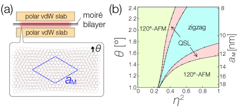
Figure 1: (a) Schematic figure of cavity moiré materials. Electrons in a moiré bilayer are ultrastrongly coupled to hyperbolic phonon polaritons confined in the cavity consisting of polar vdW crystals such as h-BN. The bottom panel shows a moiré superlattice with lattice constant $a_{M}$ formed by a bilayer with twist angle $\theta$. (b) Ground-state phase diagram of the cavity-confined TMD heterobilayer at half-filling plotted against $\theta$ and dimensionless light-matter coupling strength $\eta$. Tuning $\eta$ and $\theta$, one can control various correlated phases, such as the 120^∘-antiferromagnetic (AFM) phase, the zigzag phase, and a candidate quantum spin liquid (QSL) phase.

This Letter aims to show that strong quantum light-matter interaction provides a way to control magnetic frustration in moiré materials. We develop a theory of cavity moiré materials to describe the interaction between electrons in a twisted bilayer and quantized electromagnetic fields inside a cavity (Fig. 1(a)). A key point is that, unlike isolated flat-band systems, moiré materials are inherently multiband systems with large interlayer contributions in tensor Berry connections Törmä et al. (2022); Topp et al. (2021). We show that this quantum geometric effect causes vacuum-induced virtual electronic transitions between flat bands and the other bands, leading to the renormalization of single-electron energies in flat bands. While such vacuum-induced modification is usually irrelevant in conventional materials, we point out that it becomes important in moiré materials because of their extremely narrow bandwidths.

We demonstrate that this electromagnetic vacuum dressing allows for controlling a variety of correlated phases of moiré materials, some of which remain elusive in current experiments. Specifically, we apply our theory to a TMD moiré heterobilayer encapsulated by ultrathin hexagonal boron nitride (h-BN) slabs (Fig. 1(a)), where light-matter coupling strength $\eta$ can be tuned by varying h-BN thicknesses. At small twist angle $\theta$ and half-filling, low-energy physics of the flat-band electrons can be described by the spin-$1/2$ antiferromagnetic (AFM) Heisenberg model on the triangular moiré lattice Wu et al. (2018); Downing et al. (2019); MacDonald et al. (1988). When placed inside the cavity, vacuum fluctuations appreciably renormalize the single-electron energies and induce long-range electron hoppings. As a result, the cavity confinement enhances the spin frustration in the Heisenberg model and allows one to control various phases including the 120^∘-AFM phase and the zigzag phase (Fig. 1(b)). Notably, in the intermediate regions, one may even realize a QSL phase of the triangular Heisenberg model, whose nature has been recently under debate Arovas et al. (2022); Zhu and White (2015); Gong et al. (2019); Hu et al. (2019); Szasz et al. (2020); Drescher et al. (2022). We expect that these predictions are within experimental reach owing to recent developments demonstrating ultrasmall mode volumes of hyperbolic polaritons in nanostructured materials Caldwell et al. (2014); Dai et al. (2014); Giles et al. (2018); Dai et al. (2019); Ma et al. (2022); Sheinfux et al. (2022).

Model.— To be concrete, we focus on a cavity confinement of twisted TMD heterobilayer WSe₂/MoSe₂, while our theoretical formulation can be generally applied to other moiré materials SM (1). Due to the spin-orbit coupling, the valence bands of each monolayer have two band maxima at different valleys with opposite spin degrees of freedom (Fig. 2(a)) Xiao et al. (2012); Wu et al. (2018). Since the valence band maxima (VBM) of monolayer WSe₂ are located in the band gap of MoSe₂ Zhang et al. (2016b), we can analyze the bilayer in terms of the VBM electrons in WSe₂ provided that the chemical potential is appropriately tuned (red dashed line in Fig. 2(a)) Wu et al. (2018); Carr et al. (2020).

When the TMD bilayer is twisted with small angle $\theta$, a triangular moiré superlattice with lattice constant $a_{M}\!\approx\!a_{0}/\theta$ is formed (see Fig. 1(a)), where $a_{0}\!\simeq\!3.32$ Å is the monolayer lattice constant of WSe₂. The effect of the moiré superlattice can be described by an effective single-particle potential $\Delta(\bm{r})$, which has the same periodicity as the moiré superlattice Wu et al. (2018); Carr et al. (2020). The low-energy Hamiltonian of the VBM electrons thus reads

$$\hat{H}_{0} =-\frac{\hat{\bm{p}}^{2}}{2m^{*}}+\Delta(\hat{\bm{r}}),$$ (1)

where $m^{*}$ is the effective mass in the valence band of WSe₂, and the moiré potential $\Delta(\bm{r})$ is given by

$$\Delta(\bm{r})=\sum_{j=1}^{6}w_{j}e^{i\bm{b}_{j}\bm{r}}.$$ (2)

Here, $\bm{b}_{j}$ is the reciprocal lattice vector of the moiré superlattice corresponding to $(j-1)\pi/3$-rotation of $4\pi/(\sqrt{3}a_{M})\bm{e}_{x}$. Since $\Delta(\bm{r})$ is real-valued and satisfies the threefold-rotational symmetry, the coefficients $w_{j}$ can be parametrized as $w_{j}=we^{-i(-1)^{j}\psi}$. We show typical band dispersions $\varepsilon_{n\bm{k}}$ on the moiré Brillouin Zone (mBZ) in Fig. 2(b), where the nearly flat band $(n\!=\!0)$ is located above the other bands $(n\!\geq\!1)$. Due to the nontrivial quantum geometry of moiré bands, the electron momentum $\hat{\bm{p}}$ has nonvanishing interband matrix elements Törmä et al. (2022); Topp et al. (2021), which facilitate the couplings to quantized dynamical electromagnetic fields as detailed later.

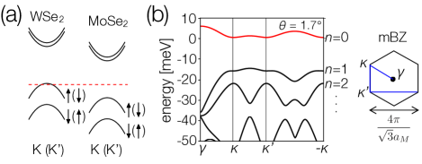
Figure 2: (a) Schematic band dispersions of monolayer WSe₂ and MoSe₂. The valence band maxima (VBM) of WSe₂ at different valleys with the opposite spin are located in the band gap of MoSe₂. The red dashed line represents the Fermi level. (b) Moiré bands of Eq. (1) at $\theta=1.7^{\circ}$. The nearly flat band with $n=0$ is highlighted by red color. The right panel shows representative points on the moiré Brillouin zone (mBZ). Parameters are $(w,\psi)=(6.6\ {\rm meV},-94^{\circ})$ and $m^{*}=0.35m_{e}$, where $m_{e}$ is the electron mass Wu et al. (2018).

The total Hamiltonian of the cavity-confined bilayer is then given by

$$\hat{H}= \sum_{\sigma}\int\!d^{2}\bm{r}\ \hat{\psi}_{\sigma\bm{r}}^{\dagger}\left[-\frac{(-i\hbar\nabla+e\hat{\bm{A}}(\bm{r}))^{2}}{2m^{*}}\!+\!\Delta(\bm{r})\right]\hat{\psi}_{\sigma\bm{r}}$$

$$+\sum_{\bm{q}}\hbar\omega_{\bm{q}}\hat{a}_{\bm{q}}^{\dagger}\hat{a}_{\bm{q}}+\hat{U},$$ (3)

where $\hat{\psi}_{\sigma\bm{r}}$ ($\hat{\psi}_{\sigma\bm{r}}^{\dagger}$) is the annihilation (creation) operator of electrons with spin $\sigma$ at position $\bm{r}$, $\hat{U}$ is the Coulomb interaction, $\hat{a}_{\bm{q}}$ ($\hat{a}_{\bm{q}}^{\dagger}$) is the annihilation (creation) operator of hyperbolic polaritons with in-plane momentum $\bm{q}$, and $\omega_{\bm{q}}$ is the mode frequency. The vector potential $\hat{\bm{A}}(\bm{r})$ is

$$\hat{\bm{A}}(\bm{r})=\sum_{\bm{q}}A_{\bm{q}}\bm{e}_{\bm{q}}(\hat{a}_{\bm{q}}e^{i\bm{q}\bm{r}}+\hat{a}_{\bm{q}}^{\dagger}e^{-i\bm{q}\bm{r}}),$$ (4)

where $A_{\bm{q}}$ is the mode amplitude of the electromagnetic component of polaritons, and $\bm{e}_{\bm{q}}\!\equiv\!\bm{q}/|\bm{q}|$ is the effective polarization obtained after projecting the originally transverse 3D vector field onto the 2D plane where the bilayer is located. We define the integrated dimensionless coupling strength by $\eta\!\equiv\!\sqrt{\sum_{\bm{q}}g_{\bm{q}}^{2}/\omega_{\bm{q}}^{2}}$, where $g_{\bm{q}}\!\equiv\!eA_{\bm{q}}\sqrt{\omega_{\bm{q}}/m^{*}\hbar}$ is the coupling strength between electrons and each cavity mode. The value of $\eta$ can reach up to $\eta\sim 1$ provided that thicknesses of h-BN slabs are tuned to be a few nanometers Ashida et al. .

Effective Hamiltonian of flat-band electrons.— We are now in a position to derive the effective Hamiltonian of flat-band electrons. To this end, we first note that the cavity frequency, which is an order of optical phonon frequency in vdW crystals $\hbar\omega_{\bm{q}}=\!10^{2}\!\sim\!10^{3}$ meV, is much larger than band gaps in the twisted bilayer (cf. Fig. 2(b)). We can thus adiabatically eliminate the cavity modes and include their vacuum fluctuations by performing the second-order perturbation with respect to $\eta$. Using simplifications that are valid in moiré flat-band systems SM (1), we obtain the effective Hamiltonian of cavity moiré materials, which is one of the main results in this Letter:

$$\hat{H}_{\rm eff} =\sum_{\bm{k}\sigma}(\varepsilon_{0\bm{k}}+\eta^{2}\xi_{\bm{k}})\hat{c}_{\bm{k}\sigma}^{\dagger}\hat{c}_{\bm{k}\sigma}+\hat{U},$$ (5)

$$\xi_{\bm{k}} \equiv\frac{m^{*}}{2\hbar^{2}}\left(-|\bm{G}_{00}^{\bm{k}}|^{2}+\sum_{n\geq 1}\frac{\hbar\omega_{\bm{0}}}{\hbar\omega_{\bm{0}}+\varepsilon_{0\bm{k}}-\varepsilon_{n\bm{k}}}|\bm{G}_{0n}^{\bm{k}}|^{2}\right),$$ (6)

where $\hat{c}_{\bm{k}\sigma}^{(\dagger)}$ is the annihilation (creation) operator of $n=0$ flat-band electrons with the Bloch wavevector $\bm{k}$ and spin $\sigma$. Remarkably, the effect of light-matter interactions is simply represented by the energy dressing $\eta^{2}\xi_{\bm{k}}$ characterized by the multiband coefficients $\bm{G}_{mn}^{\bm{k}}\equiv\langle u_{m\bm{k}}|\nabla_{\bm{k}}\hat{H}_{0\bm{k}}|u_{n\bm{k}}\rangle$, where $|u_{n\bm{k}}\rangle$ is the Bloch eigenstate of $\hat{H}_{0\bm{k}}\!\equiv\!e^{-i\bm{k}\hat{\bm{r}}}\hat{H}_{0}e^{i\bm{k}\hat{\bm{r}}}$ with band index $n$.

From a quantum geometrical viewpoint, the multiband coefficients can be expressed as

$$\bm{G}_{mn}^{\bm{k}}=\delta_{mn}\nabla_{\bm{k}}\varepsilon_{n\bm{k}}+i(\varepsilon_{m\bm{k}}-\varepsilon_{n\bm{k}}){\mathcal{A}}_{mn}(\bm{k})$$ (7)

with ${\mathcal{A}}_{mn}(\bm{k})=i\langle u_{m\bm{k}}|\nabla u_{n\bm{k}}\rangle$ being the tensor Berry connections. In moiré materials, ${\mathcal{A}}_{mn}$ has large interband contributions, while $\nabla_{\bm{k}}\varepsilon_{0\bm{k}}$ vanishes in the flat-band limit. Thus, the renormalization $\xi_{\bm{k}}$ in Eq. (6) is mainly attributed to its second term originating from virtual interband transitions induced by the vacuum fluctuations in the cavity. We note that this key multiband process cannot be captured in an oversimplified description of cavity materials, such as the Peierls substitution of the single-band tight-binding model.

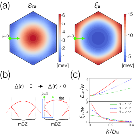
Figure 3: (a) Typical moiré flat-band dispersion $\varepsilon_{0\bm{k}}$ (left panel) and cavity renormalization $\xi_{\bm{k}}$ in Eq. (6) (right panel) on the mBZ with $\theta\!=\!1.7^{\circ}$ and $\hbar\omega_{\bm{0}}\!=\!10^{2}$ meV. (b) Schematic figure illustrating the formation of the moiré flat band. (c) Band dispersion $\varepsilon_{+k}$ and cavity renormalization $\xi_{k}$ (Eqs. (9) and (10)) of the two-band Hamiltonian (8) plotted against $k/b_{M}$ with $b_{M}=4\pi/(\sqrt{3}a_{M})$, where $k\!=\!0$ corresponds to the edge of the mBZ as indicated in (a) and (b).

General properties in cavity moiré materials.— To reveal generic features of cavity moiré materials, in Fig. 3(a) we show typical bare dispersion $\varepsilon_{0\bm{k}}$ of the nearly flat band and the corresponding cavity renormalization $\xi_{\bm{k}}$ on the mBZ. Interestingly, the dispersions of $\varepsilon_{0\bm{k}}$ and $\xi_{\bm{k}}$ are opposite each other, namely, $\varepsilon_{0\bm{k}}$ ($\xi_{\bm{k}}$) takes the largest value at the center (edge) of the mBZ. Moreover, the contributions of $\xi_{\bm{k}}$ are tightly localized around the edge of the mBZ, which can be translated to the emergence of long-range electron hoppings in real-space basis.

These key features can be qualitatively understood by analyzing a simple two-band model. In the TMD bilayer, the original monolayer band around VBM is first folded into the mBZ (left panel in Fig. 3(b)) in accordance with the change of the lattice constant from $a_{0}$ to $a_{M}$. The degeneracy at the edge of the mBZ is then lifted by the moiré potential $\Delta(\bm{r})$, leading to the nearly flat moiré band (right panel in Fig. 3(b)). We can thus describe the energy bands near the mBZ edge by the following two-band Hamiltonian:

$$\mathcal{H}(k)=\hbar v_{F}k\hat{\sigma}_{z}+w\hat{\sigma}_{x},$$ (8)

where $\hat{\sigma}_{i}$ is the Pauli matrix, $k$ is the wavevector measured from the edge of the mBZ, $v_{F}$ is the Fermi velocity at the mBZ edge (cf. left panel in Fig. 3(b)), and $w\!=\!|w_{j}|$ is the depth of the moiré potential in Eq. (2). Using the two-band model (8), the energy dispersions $\varepsilon_{\pm k}$ and the cavity renormalization $\xi_{k}$ can be obtained as

$$\varepsilon_{\pm k} =\pm w\sqrt{1+\left(\frac{\hbar v_{F}k}{w}\right)^{2}},$$ (9)

$$\xi_{k} =\frac{m^{*}v_{F}^{2}}{1+\left(\frac{\hbar v_{F}k}{w}\right)^{2}}+{\rm const.}$$ (10)

As shown in Fig. 3(c), $\varepsilon_{+k}$ ($\xi_{k}$) takes the smallest (largest) value at the edge of the mBZ, which correctly reproduces the qualitative features in Fig. 3(a). Also, $\xi_{k}$ in Eq. (10) is localized around $k\!=\!0$ with a width $\Delta k\!\sim\!w/(\hbar v_{F})\propto\theta^{-1}$ (cf. Fig. 3(c)). In real space, this leads to a long-distance hopping whose range is proportional to $\theta$. In general, such long-range contribution can generate strong magnetic frustration and is expected to qualitatively affect the ground-state properties as discussed below.

Tight-binding description and the spin model.— Using the Wannier basis, we can rewrite the effective Hamiltonian (5) by the following Hubbard model on the moiré triangular lattice:

$$\hat{H}_{\rm eff} =\sum_{ij,\sigma}t_{ij}\hat{c}_{i\sigma}^{\dagger}\hat{c}_{j\sigma}+U\sum_{i}\hat{n}_{i\uparrow}\hat{n}_{i\downarrow},$$ (11)

$$t_{ij} =\int_{\rm mBZ}\frac{v_{M}d^{2}\bm{k}}{(2\pi)^{2}}(\varepsilon_{0\bm{k}}+\eta^{2}\xi_{\bm{k}})e^{i\bm{k}(\bm{R}_{i}-\bm{R}_{j})}$$ (12)

$$\equiv\tilde{\varepsilon}_{ij}+\eta^{2}\tilde{\xi}_{ij},$$ (13)

where $\hat{c}_{i\sigma}^{(\dagger)}$ is the annihilation (creation) operator of the Wannier orbital localized at $\bm{R}_{i}$, $v_{M}$ is the volume of the moiré supercell, and we simplify the Coulomb repulsion by the on-site interaction $U\sum_{i}\hat{n}_{i\uparrow}\hat{n}_{i\downarrow}$. Let us represent the hoppings $t_{ij}$ to the $n$-th nearest neighbors (NNs) by $t_{n}$ and neglect the amplitudes $t_{n}$ with $n\!\geq\!4$, which are sufficiently small when $\theta\lesssim 2.5^{\circ}$. Since the parameters satisfy $t_{n}\ll U$ Wu et al. (2018), at half-filling, we can further simplify the Hubbard model (11) to the triangular AFM Heisenberg model MacDonald et al. (1988):

$$\hat{H}_{\rm AFM} =\sum_{1\text{st NN}}J_{1}\hat{\bm{s}}_{i}\!\cdot\!\hat{\bm{s}}_{j}+\sum_{2\text{nd NN}}J_{2}\hat{\bm{s}}_{i}\!\cdot\!\hat{\bm{s}}_{j}+\sum_{3\text{rd NN}}J_{3}\hat{\bm{s}}_{i}\!\cdot\!\hat{\bm{s}}_{j},$$ (14)

where $\hat{\bm{s}}_{i}$ is the spin-$1/2$ operator at the $i$-th site, and $J_{n}\equiv 4t_{n}^{2}/U$. This frustrated spin model has been studied in, e.g., Refs. Zhu and White (2015); Gong et al. (2019); Hu et al. (2019); Szasz et al. (2020); Drescher et al. (2022), and a nonmagnetic insulating phase, which is a candidate QSL phase, is found in the parameter region around $J_{2}/J_{1}\!\sim\!0.3$ and $J_{3}/J_{1}\!\sim\!0.15$ Gong et al. (2019).

One of our main findings is the possibility of controlling such spin frustration by the cavity confinement. Specifically, one can tune the light-matter coupling strength $\eta$ to enhance the hopping amplitudes $t_{n}$ to distant sites ($n\!=\!2,3$) while suppressing the NN hopping $t_{1}$ (Fig. 4(b)). Physically, this tunability originates from the opposite dispersions in $\varepsilon_{0\bm{k}}$ and $\xi_{\bm{k}}$ described above (Fig. 3(a)), which correspond to the opposite signs of their Fourier transforms, $\tilde{\varepsilon}_{n}$ and $\tilde{\xi}_{n}$, that are related to the renormalized hopping via $t_{n}=\tilde{\varepsilon}_{n}+\eta^{2}\tilde{\xi}_{n}$. We show the corresponding $\eta$-dependence of $J_{2}/J_{1}$ and $J_{3}/J_{1}$ in Fig. 4(c), where one can realize particularly large spin-coupling ratios $J_{n}/J_{1}$ when the NN coupling $J_{1}$ becomes vanishingly small. Comparing with the numerical results in the triangular AFM Heisenberg model Gong et al. (2019), we determine the ground-state phase diagram of the present cavity moiré system as in Fig. 1(b). The key finding is that the high tunability of $\eta$ and $\theta$ should allow for controlling various correlated phases including a candidate QSL phase.

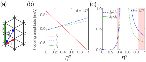
Figure 4: (a) First-, second-, and third-order nearest neighbors (NNs) on the moiré triangular lattice. (b) Renormalized hopping amplitudes $t_{n}$ to the $n$-th NNs and (c) corresponding spin-coupling ratios $J_{i}/J_{1}$ ($i=2,3$) in the triangular AFM Heisenberg model (14) plotted against the light-matter coupling strength at $\theta\!=\!1.7^{\circ}$. The red shaded areas in (c) indicate the intermediate parameter regions where the ground state is expected to be a quantum spin liquid.

Discussions.— We recall that a central feature of cavity moiré materials is the renormalization of single-electron energies in flat bands, which is induced by the virtual interband transitions originating from the nontrivial quantum geometry of moiré bands (cf. Eqs. (6) and (7)). While vacuum fluctuations can also induce the Amperean electron-electron interaction Schlawin et al. (2019), we note that this contribution is negligibly small compared to the Coulomb interaction due to the flatness of moiré bands SM (1). In contrast, a usual monolayer has dispersive bands and band gap is typically much larger than a resonance frequency of the h-BN cavity considered here. Thus, if monolayer is confined in the vdW slabs, the Amperean paring term could be also relevant.

In summary, we developed a theory of moiré materials strongly coupled to quantized electromagnetic fields inside a cavity. We showed that the major effect of the cavity confinement is the renormalization of the single-electron energies in flat bands. Physically, this originates from the nontrivial quantum geometry of the moiré bands, which leads to virtual interband electronic transitions induced by electromagnetic vacuum fluctuations. The resulting long-range electronic hoppings allow for tuning the spin frustration in the low-energy effective model, thus suggesting the possibility of controlling correlated phases with quantum light-matter interaction. We analyzed the concrete setup consisting of TMD heterobilayer WSe₂/MoSe₂ confined in the h-BN cavity, and revealed that various phases, including a putative QSL state, can be realized by varying the light-matter coupling strength $\eta$ (Fig. 1(b)). Our findings are of experimental relevance in view of recent developments demonstrating ultrasmall mode volumes of hyperbolic polaritons in nanostructured materials Caldwell et al. (2014); Dai et al. (2014); Giles et al. (2018); Dai et al. (2019); Ma et al. (2022); Sheinfux et al. (2022).

Several open questions remain for future studies. In the present perturbation theory, we only retain the leading terms of ${\rm O}(\eta^{2})$, while the higher-order corrections might be important especially when $\eta={\rm O}(1)$. It would be interesting to analyze such a challenging regime on the basis of a nonperturbative approach allowing for nonvanishing electron-photon entanglement Wang et al. (2021); Ashida et al. (2021). It is also worthwhile to recall that the cavity-mediated hoppings $\eta^{2}\tilde{\xi}_{ij}$ in Eq. (5) become more long-ranged as twist angle $\theta$ is increased. It merits further study to examine these large-$\theta$ regimes of cavity moiré materials beyond the parameter region considered here Liao et al. (2020); Zhang et al. (2020b); Tao et al. (2022); there, higher-order hoppings $t_{n}$ should be increasingly important and an effective Hamiltonian may exhibit stronger magnetic frustration in which the ground-state phase diagram could be enriched. We hope that our work simulates further studies in these directions.

Supplementary Materials

.1 Derivation of the effective Hamiltonian of flat-band electrons

We here provide the derivation of the effective Hamiltonian of flat-band electrons (5) in the main text. Specifically, we start from the cavity moiré Hamiltonian given by (see Eq. (3) in the main text)

$$\hat{H} =\sum_{\sigma}\int\!d^{2}\bm{r}\ \hat{\psi}_{\sigma\bm{r}}^{\dagger}\left[-\frac{(-i\hbar\nabla+e\hat{\bm{A}}(\bm{r}))^{2}}{2m^{*}}\!+\!\Delta(\bm{r})\right]\hat{\psi}_{\sigma\bm{r}}+\sum_{\bm{q}}\hbar\omega_{\bm{q}}\hat{a}_{\bm{q}}^{\dagger}\hat{a}_{\bm{q}}+\hat{U},$$ (S1)

$$\hat{\bm{A}}(\bm{r}) =\sum_{\bm{q}}A_{\bm{q}}\bm{e}_{\bm{q}}(\hat{a}_{\bm{q}}e^{i\bm{q}\bm{r}}+\hat{a}_{\bm{q}}^{\dagger}e^{-i\bm{q}\bm{r}}).$$ (S2)

For the sake of generality, we consider the band structure shown in Fig. S1(a) as the dispersions $\varepsilon_{n\bm{k}}$ of the bare moiré Hamiltonian $\hat{H}_{0}\!\equiv\!-\hat{\bm{p}}^{2}/2m^{*}+\Delta(\bm{r})$, where the flat band (labelled by $n=0$) is located between the other electronic bands ($n\neq 0$). Since band gaps in moiré materials are much smaller than the cavity frequencies, the low-energy states of cavity moiré Hamiltonian (S1) can be approximated by a product state $|\psi_{\rm e}\rangle\otimes|0\rangle$, where $|0\rangle$ is the electromagnetic vacuum, and $|\psi_{\rm e}\rangle$ is an electronic state with the partially-filled flat band and occupied (unoccupied) lower (upper) bands (cf. Fig. S1(b)). We define the projection operator $\hat{P}$ onto the manifold spanned by these states and obtain the effective Hamiltonian in this subspace by employing the perturbation theory with respect to the (dimensionless) light-matter coupling strength $\eta=\sqrt{\sum_{\bm{q}}g_{\bm{q}}^{2}/\omega_{\bm{q}}^{2}}$.

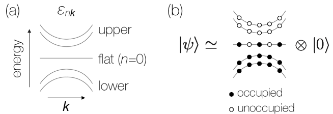
Figure S1: (a) Schematic band dispersions of a moiré Hamiltonian $\hat{H}_{0}=-\hat{\bm{p}}^{2}/2m^{*}+\Delta(\bm{r})$, where the flat band is located between the other electronic bands. (b) Approximate low-energy states $|\psi\rangle\simeq|\psi_{\rm e}\rangle\otimes|0\rangle$ consisting of the product between the electromagnetic vacuum $|0\rangle$ and an electronic state $|\psi_{\rm e}\rangle$ with the partially filled flat band and occupied (unoccupied) lower (upper) bands.

To proceed, we decompose the moiré Hamiltonian (S1) as

$$\hat{H}= \hat{H}_{0}+\sum_{\bm{q}}\hbar\omega_{\bm{q}}^{\prime}\hat{a}_{\bm{q}}^{\dagger}\hat{a}_{\bm{q}}+\hat{H}_{I}^{(p)}+\hat{H}_{I}^{(q)}+\hat{U},$$ (S3)

$$\omega_{\bm{q}}^{\prime}= \omega_{\bm{q}}\left(1+\frac{N_{e}e^{2}A_{\bm{q}}^{2}}{m^{*}\hbar\omega_{\bm{q}}}\right)=\omega_{\bm{q}}\left(1+\frac{N_{e}g_{\bm{q}}^{2}}{\omega_{\bm{q}}^{2}}\right),$$ (S4)

$$\hat{H}_{I}^{(p)}= -\sum_{\bm{q}}\frac{eA_{\bm{q}}}{m^{*}}\left(\sum_{\sigma}\int d^{2}{\bm{r}}\ \hat{\psi}_{\sigma\bm{r}}^{\dagger}\frac{(\hat{\bm{p}}\!\cdot\!\bm{e}_{\bm{q}})e^{i\bm{q}\bm{r}}+e^{i\bm{q}\bm{r}}(\hat{\bm{p}}\!\cdot\!\bm{e}_{\bm{q}})}{2}\hat{\psi}_{\sigma\bm{r}}\right)\hat{a}_{\bm{q}}+{\rm H.c.},$$ (S5)

$$\hat{H}_{I}^{(q)}= \sum_{\bm{q}_{1},\bm{q}_{2}}\sum_{\sigma}\int d^{2}{\bm{r}}\ \hat{\psi}_{\sigma\bm{r}}^{\dagger}\frac{e^{2}A_{\bm{q}_{1}}A_{\bm{q}_{2}}}{2m^{*}}\bm{e}_{\bm{q}_{1}}\!\cdot\!\bm{e}_{\bm{q}_{2}}(\hat{a}_{\bm{q}_{1}}\hat{a}_{\bm{q}_{2}}e^{i(\bm{q}_{1}+\bm{q}_{2})\bm{r}}+{\rm H.c.})\ \hat{\psi}_{\sigma\bm{r}}$$

$$+\sum_{\bm{q}_{1}\neq\bm{q}_{2}}\sum_{\sigma}\int d^{2}{\bm{r}}\ \hat{\psi}_{\sigma\bm{r}}^{\dagger}\frac{e^{2}A_{\bm{q}_{1}}A_{\bm{q}_{2}}}{2m^{*}}\bm{e}_{\bm{q}_{1}}\!\cdot\!\bm{e}_{\bm{q}_{2}}(\hat{a}_{\bm{q}_{1}}^{\dagger}\hat{a}_{\bm{q}_{2}}e^{-i(\bm{q}_{1}-\bm{q}_{2})\bm{r}}+{\rm H.c.})\ \hat{\psi}_{\sigma\bm{r}},$$ (S6)

where $\hat{H}_{I}^{(p)}$ is the paramagnetic term, and the $A^{2}$ diamagnetic term leads to the renormalized cavity frequency $\omega_{\bm{q}}^{\prime}$ and the interaction term $\hat{H}_{I}^{(q)}$. In Eq. (S4), we define the total number of electrons by $N_{e}=\sum_{\sigma}\int d^{2}{\bm{r}}\hat{\psi}_{\sigma\bm{r}}^{\dagger}\hat{\psi}_{\sigma\bm{r}}$, which is an order of $V/v_{M}$ with the system size $V$ and the volume of the moiré supercell $v_{M}$. Since the coupling strength $g_{\bm{q}}$ is proportional to $\sqrt{1/V}$, the frequency renormalization in Eq. (S4) is ${\rm O}(V^{0}\eta^{2})$. Below, we treat the first two terms in the right hand side of Eq. (S3) as the unperturbed Hamiltonian and incorporate the effect of $\hat{H}_{I}^{(p)}+\hat{H}_{I}^{(q)}$ by the perturbation theory.

Since $\hat{P}\hat{H}_{I}^{(p)}\hat{P}=\hat{P}\hat{H}_{I}^{(q)}\hat{P}=0$, the leading terms come from the second-order perturbation of the paramagnetic term $\hat{H}_{I}^{(p)}$, which can be expressed in the Bloch basis as

$$\hat{H}_{I}^{(p)} =-\sum_{\bm{k}\sigma}\sum_{mn}\sum_{\bm{q}}\frac{eA_{\bm{q}}}{m^{*}}\bm{e}_{\bm{q}}\!\cdot\!\langle\psi_{m\bm{k}+\bm{q}\sigma}|\frac{\hat{\bm{p}}e^{i\bm{q}\bm{r}}+e^{i\bm{q}\bm{r}}\hat{\bm{p}}}{2}|\psi_{n\bm{k}\sigma}\rangle\hat{c}_{m\bm{k}+\bm{q}\sigma}^{\dagger}\hat{c}_{n\bm{k}\sigma}\hat{a}_{\bm{q}}+{\rm H.c.}$$ (S7)

$$=-\sum_{\bm{k}\sigma}\sum_{mn}\sum_{\bm{q}}\frac{eA_{\bm{q}}}{m^{*}}\bm{e}_{\bm{q}}\!\cdot\!\langle u_{m\bm{k}+\bm{q}}|\left(\hat{\bm{p}}+\hbar\left(\bm{k}+\frac{\bm{q}}{2}\right)\right)|u_{n\bm{k}}\rangle\hat{c}_{m\bm{k}+\bm{q}\sigma}^{\dagger}\hat{c}_{n\bm{k}\sigma}\hat{a}_{\bm{q}}+{\rm H.c.}$$ (S8)

$$=-\sum_{\bm{k}\sigma}\sum_{mn}\sum_{\bm{q}}\frac{eA_{\bm{q}}}{\hbar}(\bm{G}_{mn}^{\bm{k},\bm{q}}\!\cdot\!\bm{e}_{\bm{q}})\ \hat{c}_{m\bm{k}+\bm{q}\sigma}^{\dagger}\hat{c}_{n\bm{k}\sigma}\hat{a}_{\bm{q}}+{\rm H.c.}$$ (S9)

Here, we introduce the annihilation (creation) operator $\hat{c}_{n\bm{k}\sigma}^{(\dagger)}$ corresponding to the Bloch state $|\psi_{n\bm{k}\sigma}\rangle$ with the spin index $\sigma$ and also define the multiband coefficients $\bm{G}_{mn}^{\bm{k},\bm{q}}\equiv\langle u_{m\bm{k}+\bm{q}}|\nabla_{\bm{k}}\hat{H}_{\bm{k}+\bm{q}/2}|u_{n\bm{k}}\rangle$, where $|u_{n\bm{k}}\rangle$ is related to $|\psi_{n\bm{k}\sigma}\rangle$ via $|\psi_{n\bm{k}\sigma}\rangle\!=\!e^{i\bm{k}\hat{\bm{r}}}|u_{n\bm{k}}\rangle\!\otimes\!|\sigma\rangle$ with spin state $|\sigma\rangle$. Figures S2(a)-(c) show the virtual processes relevant to the second-order perturbation of $\hat{H}_{I}^{(p)}$, each of which corresponds to the virtual electronic transitions (a) within the flat band, (b) to the upper bands, and (c) from the lower bands, respectively. Approximating the excitation energy $\Delta E$ in each process as shown in Fig. S2, we get the following effective Hamiltonian of flat-band electrons:

$$\hat{H}_{\rm eff}= \sum_{\bm{k}\sigma}\varepsilon_{0\bm{k}}\hat{c}_{\bm{k}\sigma}^{\dagger}\hat{c}_{\bm{k}\sigma}+\hat{H}_{\rm ff}+\hat{H}_{\rm fu}+\hat{H}_{\rm fl}+\hat{U},$$ (S10)

$$\hat{H}_{\rm ff}= -\sum_{\bm{k},\bm{k}^{\prime}}\sum_{\sigma,\sigma^{\prime}}\sum_{\bm{q}}\frac{m^{*}}{\hbar^{2}}\frac{g_{\bm{q}}^{2}}{{\omega^{\prime}_{\bm{q}}}^{2}}(\bm{G}_{00}^{\bm{k},\bm{q}}\!\cdot\!\bm{e}_{\bm{q}})(\bm{G}_{00}^{\bm{k}^{\prime},\bm{q}*}\!\cdot\!\bm{e}_{\bm{q}})\hat{c}_{\bm{k}+\bm{q}\sigma}^{\dagger}\hat{c}^{\dagger}_{\bm{k}^{\prime}-\bm{q}\sigma^{\prime}}\hat{c}_{\bm{k}^{\prime}\sigma^{\prime}}\hat{c}_{\bm{k}\sigma}$$

$$-\sum_{\bm{k}\sigma}\frac{m^{*}}{\hbar^{2}}\left(\sum_{\bm{q}}\frac{g_{\bm{q}}^{2}}{{\omega^{\prime}_{\bm{q}}}^{2}}|\bm{G}_{00}^{\bm{k},\bm{q}}\!\cdot\!\bm{e}_{\bm{q}}|^{2}\right)\hat{c}_{\bm{k}\sigma}^{\dagger}\hat{c}_{\bm{k}\sigma},$$ (S11)

$$\hat{H}_{\rm fu}= -\sum_{\bm{k}\sigma}\frac{m^{*}}{\hbar^{2}}\left(\sum_{\bm{q}}\sum_{n}^{\rm upper}\frac{g_{\bm{q}}^{2}}{{\omega^{\prime}_{\bm{q}}}^{2}}\frac{\hbar\omega_{\bm{q}}^{\prime}}{\hbar\omega_{\bm{q}}^{\prime}+\varepsilon_{n\bm{k}+\bm{q}}-\varepsilon_{0\bm{k}}}|\bm{G}_{n0}^{\bm{k},\bm{q}}\!\cdot\!\bm{e}_{\bm{q}}|^{2}\right)\hat{c}_{\bm{k}\sigma}^{\dagger}\hat{c}_{\bm{k}\sigma},$$ (S12)

$$\hat{H}_{\rm fl}= \sum_{\bm{k}\sigma}\frac{m^{*}}{\hbar^{2}}\left(\sum_{\bm{q}}\sum_{n}^{\rm lower}\frac{g_{\bm{q}}^{2}}{{\omega^{\prime}_{\bm{q}}}^{2}}\frac{\hbar\omega_{\bm{q}}^{\prime}}{\hbar\omega_{\bm{q}}^{\prime}+\varepsilon_{0\bm{k}}-\varepsilon_{n\bm{k}+\bm{q}}}|\bm{G}_{0n}^{\bm{k},\bm{q}}\!\cdot\!\bm{e}_{\bm{q}}|^{2}\right)\hat{c}_{\bm{k}\sigma}^{\dagger}\hat{c}_{\bm{k}\sigma},$$ (S13)

where $\hat{c}_{\bm{k}\sigma}^{(\dagger)}=\hat{c}_{0\bm{k}\sigma}^{(\dagger)}$ is the annihilation (creation) operator of the flat-band electrons, and $\sum_{n}^{\rm upper(lower)}$ denotes the summation over the upper (lower) bands. In deriving Eqs. (S11)-(S13), we assume the relations $g_{\bm{q}}=g_{-\bm{q}}$ and $\omega_{\bm{q}}^{\prime}=\omega^{\prime}_{-\bm{q}}$ that hold true for uniaxial cavities, and use the following equalities:

$$\hat{P}(\hat{c}_{0\bm{k}\sigma}^{\dagger}\hat{c}_{n\bm{k}+\bm{q}\sigma}\hat{c}_{n^{\prime}\bm{k}^{\prime}+\bm{q}\sigma^{\prime}}^{\dagger}\hat{c}_{0\bm{k}^{\prime}\sigma^{\prime}})\hat{P}=\delta_{nn^{\prime}}\delta_{\bm{k}\bm{k}^{\prime}}\delta_{\sigma\sigma^{\prime}}\hat{c}_{0\bm{k}\sigma}^{\dagger}\hat{c}_{0\bm{k}\sigma}\ (n,n^{\prime}:\text{upper bands}),$$ (S14)

$$\hat{P}(\hat{c}_{n\bm{k}+\bm{q}\sigma}^{\dagger}\hat{c}_{0\bm{k}\sigma}\hat{c}_{0\bm{k}^{\prime}\sigma^{\prime}}^{\dagger}\hat{c}_{n^{\prime}\bm{k}^{\prime}+\bm{q}\sigma^{\prime}})\hat{P}=\delta_{nn^{\prime}}\delta_{\bm{k}\bm{k}^{\prime}}\delta_{\sigma\sigma^{\prime}}\hat{c}_{0\bm{k}\sigma}\hat{c}_{0\bm{k}\sigma}^{\dagger}\ (n,n^{\prime}:\text{lower bands}).$$ (S15)

We note that the first term in the right hand side of Eq. (S11) is the Amperean electron-electron interaction mediated by cavity electromagnetic fields Schlawin et al. (2019). Since the coefficients $(\bm{G}_{00}^{\bm{k},\bm{q}}\!\cdot\!\bm{e}_{\bm{q}})(\bm{G}_{00}^{\bm{k}^{\prime},\bm{q}*}\!\cdot\!\bm{e}_{\bm{q}})\approx(\nabla_{\bm{k}}\varepsilon_{0\bm{k}}\!\cdot\!\bm{e}_{\bm{q}})(\nabla_{\bm{k}}\varepsilon_{0\bm{k}^{\prime}}\!\cdot\!\bm{e}_{\bm{q}})$ in this term almost vanish due to the band flatness, the Amperean interaction is negligibly small compared to the Coulomb interaction $\hat{U}$. Retaining up to ${\rm O}(\eta^{2})$-terms and taking the limit $\bm{q}\to\bm{0}$ in Eq. (S3) (which does not affect the results provided in the present work), we finally obtain the effective Hamiltonian of flat-band electrons as

$$\hat{H}_{\rm eff} =\sum_{\bm{k}\sigma}(\varepsilon_{0\bm{k}}+\eta^{2}\xi_{\bm{k}})\hat{c}_{\bm{k}\sigma}^{\dagger}\hat{c}_{\bm{k}\sigma}+\hat{U},$$ (S16)

$$\xi_{\bm{k}} =\frac{m^{*}}{2\hbar^{2}}\left(-|\bm{G}_{00}^{\bm{k}}|-\sum_{n}^{\rm upper}\frac{\hbar\omega_{\bm{0}}}{\hbar\omega_{\bm{0}}+\varepsilon_{n\bm{k}}-\varepsilon_{0\bm{k}}}|\bm{G}_{n0}^{\bm{k}}|^{2}+\sum_{n}^{\rm lower}\frac{\hbar\omega_{\bm{0}}}{\hbar\omega_{\bm{0}}+\varepsilon_{0\bm{k}}-\varepsilon_{n\bm{k}}}|\bm{G}_{n0}^{\bm{k}}|^{2}\right),$$ (S17)

where we introduce $\bm{G}_{mn}^{\bm{k}}\equiv\bm{G}_{mn}^{\bm{k},\bm{0}}$ and use the fact that $\omega_{\bm{q}}^{\prime}/\omega_{\bm{q}}=1+{\rm O}(\eta^{2})$. Since there are no upper bands in the setup of the TMD heterobilayer considered in the main text, the effective Hamiltonian (S16) simplifies to Eq. (5) in the main text.

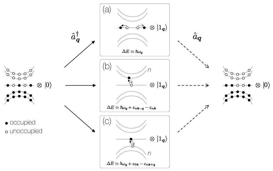
Figure S2: Virtual processes in the second-order perturbation of the paramagnetic term $\hat{H}_{I}^{(p)}$, where a cavity mode is excited by $\hat{a}_{\bm{q}}^{\dagger}$ with (a) intraband transitions within the flat band, (b) interband transitions from the flat band to an upper band, and (c) interband transitions from a lower band to the flat band. We approximate excitation energies in each process $\Delta E$ as shown in (a)-(c).

Making appropriate modifications in the moiré Hamiltonian (S1), our procedure can also be applied to other moiré materials, such as a TMD moiré homobilayer or a twisted bilayer graphene. In a TMD moiré homobilayer, the moiré Hamiltonian of spin-up electrons (or equivalently, K-valley electrons in the TMD monolayers) is given as Carr et al. (2020); Wu et al. (2019),

$$\hat{H}_{0\uparrow}=\left(\begin{array}[]{cc}-\frac{(\hat{\bm{p}}-\hbar\bm{\kappa}_{b})^{2}}{2m^{*}}&\\ &-\frac{(\hat{\bm{p}}-\hbar\bm{\kappa}_{t})^{2}}{2m^{*}}\end{array}\right)+\hat{\Delta}(\bm{r}),$$ (S20)

where the $2\!\times\!2$-matrix corresponds to the two layer degrees of freedom, and $\hat{\Delta}(\bm{r})$ is a $2\!\times\!2$-matrix-valued moiré potential. Here, $\bm{\kappa}_{t(b)}$ denotes the distinct mBZ corner, which originates from the K-valley of the top (bottom) TMD monolayer (cf. Fig. S3). The moié Hamiltonian of spin-down electrons $\hat{H}_{0\downarrow}$ is given as the time-reversal (TR) pair of $\hat{H}_{0\uparrow}$. We note that $\hat{H}_{0\uparrow(\downarrow)}$ does not have TR-symmetry $(\hat{\bm{p}},\hat{\Delta}(\bm{r}))\to(-\hat{\bm{p}},\hat{\Delta}^{*}(\bm{r}))$, while the total moiré Hamiltonian $\hat{H}_{0\uparrow}+\hat{H}_{0\downarrow}$ does $(\hat{\bm{p}},\hat{\Delta}(\bm{r}),\sigma)\to(-\hat{\bm{p}},\hat{\Delta}^{*}(\bm{r}),-\sigma)$. As a result, the hopping amplitudes $t_{ij,\sigma}$ in the tight-binding description are in general complex-valued and satisfy $t_{ij,-\sigma}=t_{ij,\sigma}^{*}$. Similarly, in a twisted bilayer graphene, the moiré Hamiltonian of spin-up and K-valley electrons is given as Carr et al. (2020); Bistritzer and MacDonald (2011),

$$\hat{H}_{0\uparrow\rm K}=\left(\begin{array}[]{cc}v_{F}(\hat{\bm{p}}-\hbar\bm{\kappa}_{b})\!\cdot\!\hat{\bm{\sigma}}&\\ &v_{F}(\hat{\bm{p}}-\hbar\bm{\kappa}_{t})\!\cdot\!\hat{\bm{\sigma}}\\ \end{array}\right)+\hat{\Delta}(\bm{r}),$$ (S23)

where $v_{F}$ is the Fermi velocity of monolayer graphene, $\hat{\bm{\sigma}}=(\hat{\sigma}_{x},\hat{\sigma}_{y})^{T}$, and $\hat{\Delta}(\bm{r})$ is a $4\!\times\!4$-matrix-valued moiré potential corresponding to the layer and sublattice degrees of freedom.

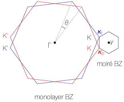
Figure S3: Moiré Brillouin Zone (mBZ) for spin-up (K-valley) electrons of TMD moiré homobilayer with twist angle $\theta$. We also show the monolayer BZ of the top (blue) and bottom (red) TMD layers.