Inferring HIV Transmission Patterns from Viral Deep-Sequence Data via Latent Typed Point Processes

Abstract

Viral deep-sequencing data play a crucial role toward understanding disease transmission network flows, because the higher resolution of these data compared to standard Sanger sequencing provide evidence into the direction of infectious disease transmission. To more fully utilize these rich data and account for the uncertainties in phylogenetic analysis outcomes, we propose a spatial Poisson process model to uncover HIV transmission flow patterns at the population level. We represent pairings of two individuals with viral sequence data as typed points, with coordinates representing covariates such as gender and age, and the point type representing the unobserved transmission statuses (linkage and direction). Points are associated with observed scores on the strength of evidence for each transmission status that are obtained through standard deep-sequenece phylogenetic analysis. Our method is able to jointly infer the latent transmission statuses for all pairings and the transmission flow surface on the source-recipient covariate space. In contrast to existing methods, our framework does not require pre-classification of the transmission statuses of data points, instead learning them probabilistically through a fully Bayesian inference scheme. By directly modeling continuous spatial processes with smooth densities, our method enjoys significant computational advantages compared to previous methods that rely on discretization of the covariate space. We demonstrate that our framework can capture age structures in HIV transmission at high resolution, and bring valuable insights in a case study on viral deep-sequencing data from Southern Uganda.

1 Introduction

As a decades-long global pandemic, the human immunodeficiency virus (HIV) has most severely affected Africa with 1 in every 25 adults living with the HIV virus, accounting for more than two-thirds of infections worldwide (Eisinger and Fauci, 2018; Fauci and Lane, 2020). International public health organizations have proposed to control the HIV epidemic by targeting intervention efforts towards populations most at risk of HIV acquisition and transmission (Glynn et al., 2001; Pettifor et al., 2008; Karim et al., 2010; Jewkes et al., 2010; Saul et al., 2018). To achieve this, it is important to understand and characterize transmission patterns between different groups and sub-populations (Wilson and Halperin, 2008).

To this end, this article proposes novel methodology to infer the relative transmission flows between different groups of individuals. Throughout this paper we will focus on heterosexual transmission flows across age groups. We model the underlying ground truth transmission flows as latent surfaces in a plane whose axes denote respectively the ages of the source and the recipient. A transmission pair is thus represented by a point on this surface with coordinates representing the phylogenetically likely source and recipient ages. The population of all transmission pairs then corresponds to a realized point pattern from the underlying flow surface. We expect that population groups with similar age attributes behave similarly, and so, in statistical terms, the underlying transmission flows can be modelled in the same way as continuous latent spatial surfaces on a compact domain specified by longitudes and latitudes (Ji et al., 2009; Kutoyants, 2012). The key scientific challenge, however, arises due to the unobserved transmission pathways in the phylogenetically likely transmission pairs—there is uncertainty about whether or not there is a transmission link, and in which direction transmission takes. Addressing the question “who infected whom?” is fundamental for inferring the population-level transmission flow.

In order to reliably infer transmission pathways between individuals, we leverage the outputs from modern phylogenetic and phylodynamic analyses using viral deep-sequencing data. Recently developed viral deep-sequencing pipelines have made it possible to estimate the linkage and direction of transmission between infected individuals (Romero-Severson et al., 2016; Leitner and Romero-Severson, 2018; Wymant et al., 2018; Ratmann et al., 2019). Multiple viral variants are observed for each individual and phylogeographic techniques can then be applied at the individual level to produce evidence about the evolutionary relationships between individual viral sequences, which inform the transmission relationships between individuals  (Wymant et al., 2018; Zhang et al., 2020). The outputs from these phylogenetic analysis pipelines typically take the form of two summary scores that represent (a) how likely deep-sequenced individuals shared a transmission link and (b) how probable transmission occurred in a specific direction. These scores can provide rich information about transmission flows between groups of individuals, for example between locations (Ratmann et al., 2020) or between age and gender groups (Bbosa et al., 2020; Xi et al., 2022; Hall et al., 2021). Importantly, the phylogenetic summary scores are imprecise at the level of two individuals and cannot be used to “prove" transmission between two individuals, because the phylogenetic signal is asssociated with measurement error and not fully consistent for the same individuals across independent evaluations on different parts of the genome (Ratmann et al., 2019; Hall et al., 2021; Zhang et al., 2020). In addition, phylogenetic analysis typically only outputs the “maximum likelihood” phylogenetic structures of viral sequences, without reporting the corresponding uncertainties for alternative structures or relationships. In practice, existing approaches for inferring population-level transmission flows neglect such uncertainty by arbitrarily thresholding the phylogenetic summary scores (e.g., by only keeping highly likely transmission pairs with likelihood scores for transmission linkage $>0.6$ and transmission direction $>0.5$, commonly called “source-recipient pairs"). As a result, the varying strengths of phylogenetic evidence are not accounted for in existing approaches. Further, a large fraction of data points are not even considered in analysis because among all pairs with some evidence of transmission, only the subset of highly likely source-recipient pairs are classified as “source-recipient pairs” and included for study. In short, there is a substantial methodological gap in existing approaches for utilizing phylogenetic evidence in that (1) differential evidence confidence is neglected and (2) a large amount of data must be discarded.

This paper addresses these limitations by proposing a coherent statistical model which jointly learns from demographic information (such as gender and age) and phylogenetic evidence. We introduce a marked latent spatial process model on the age space, where each transmission pair of individuals (represented by their paired ages as coordinates on the space) is associated with “marks” that contain the phylogenetic summary scores. That is, each potential transmission pair is assigned a latent “type" random variable that indicates the unknown transmission statuses (linkage and direction). The distribution of transmission flow between age groups and the distribution of the “marks” (phylogenetic scores) both depend on the latent type variable. We derive the likelihood of the complete model, so that basing inference in a data-augmented Bayesian framework then allows us to probabilistically learn the latent type for each potential transmission pair. In particular, this allows the evidence strength for each pair of infected individuals to be quantified— for example, we may conclude a 85% posterior probability for a specific heterosexual pair to be linked through transmission, and this pair would contribute more to the learning of transmission flow surfaces compared to another pair with a 40% posterior probability of linkage. More importantly, this joint modeling approach enables us to make use of substantially more data, as “low-confidence” pairs with lower phylogenetic scores reflecting weaker evidence for transmission linkage or direction are downweighted in a data-driven manner rather than discarded.

Not only will the latent spatial point process approach leverage more evidence with uncertainty quantification, but it also admits a more computationally efficient solution. This is largely due to the continuous formulation of the transmission flow age space. A common approach in past epidemiological studies makes use of discrete grids based on pre-specified age groups (such as 1-year or 5-year age groups), but these heuristic groupings can lead to computationally intensive downstream analysis (Hyman et al., 1994; Heuveline, 2004; Sharrow et al., 2014). For instance, recent work of Xi et al. (2022) introduces a semi-parametric Poisson model for flow counts on discrete age strata and other demographic attributes. The number of observed points is typically considerably smaller than the number of all cells in the high-dimensional age grid; those structural zeros in discrete age cells require a considerable amount of book-keeping as well as heavy computation for model smoothing. Instead, point pattern approaches with a continuous underlying flow surface can be at once more general and more computationally efficient, even with the addition of latent transmission types. These advances free us from specifying ad hoc thresholds on the phylogenetic summary scores, and in turn allow the larger set of available data points with lower evidence confidence to be considered, with each data point weighed according to its phylogenetic evidence. Interestingly, we will also show that the point process model borrows information in a two-way manner, leveraging the additional data to learn the transmission flows, and using the transmission flows to learn the point types. Although our statistical methodology is motivated by applications in HIV transmissions, it represents a general framework that can be applied to studying transmission dynamics for many other infectious diseases such as hepatitis C virus, human papillomavirus and Monkeypox virus.

Prior work

Spatial Poisson process models have been widely applied to the study of point-referenced two-dimensional data (Banerjee et al., 2003; Huber, 2011; Cressie, 2015). Heterogeneity in spatial point patterns is often modelled through non-homogeneous Poisson processes (NHPPs), where the structure of the intensity function can be described using various choices of Bayesian mixture models. NHPP intensity functions have been parameterized through Markov random fields for piecewise constant functions based on Voronoi tessellations (Heikkinen and Arjas, 1998), weighted Gamma process mixtures of non-negative kernel functions (Lo and Weng, 1989; Wolpert and Ickstadt, 1998; Ishwaran and James, 2004), Gaussian process mixtures of log-transformed components (Møller et al., 1998; Brix and Diggle, 2001; Adams et al., 2009), and Dirichlet process mixtures (Ji et al., 2009; Zhou et al., 2015; Zhao and Kottas, 2021). Kim and Kottas (2022) offer an excellent summary. Our framework builds on previous developments in Dirichlet process mixtures that focus on learning a normalized functional form of the NHPP intensity (Kottas and Sansó, 2007; Kottas et al., 2008; Taddy et al., 2012), which admits tractable and efficient inference procedures and in this application corresponds to the transmission flows that we seek to infer.

In recent years, Poisson process models have been extended to study spatial point patterns that are latent or partially observed, in that only certain indirect “signals” associated with the underlying spatial pattern are observed, with uncertainty about the quantity and locations of the latent points (Vedel Jesen and Thorarinsdottir, 2007; Ji et al., 2009). Here, a “signal” is any additional information associated with a data point in the spatial pattern, which may depend on the location of the associated spatial point. The signal can be the height of trees in a forest survey, temperature of water sample in a lake, or in our application, the phylogenetic evidence between a pair of infected individuals. Joint modelling of the signals and the latent point process through Bayesian data augmentation has been successful, thanks to the ease of incorporating missing information as latent variables in a Bayesian inference framework (Givens et al., 1997). However, to our knowledge, much of the existing work in spatial Point process models focuses on one set or type of spatial points, rather than a combination of multiple types of latent point patterns whose “types” are associated with practical interpretation, but are not observed. Our framework also bridges this methodological gap by exploiting additional signals that inform the latent type labels in a marked spatial Poisson process model.

This paper is structured as follows. We first provide an overview of the motivating data and develop the model framework in Section 2. The latent Poisson spatial process model and a likelihood-based inference scheme are presented in Section 3. We then investigate the accuracy of inference under the proposed model and its ability to differentiate between competing transmission flow hypotheses on simulate data in Section 4. Next, we illustrate the efficacy of the proposed approach on demographic and HIV deep-sequence data from the Rakai Community Cohort Study in Southern Uganda in Section 5. Finally, we discuss the merits and limitations of the proposed statistical model in Section 6.

2 Data and Model

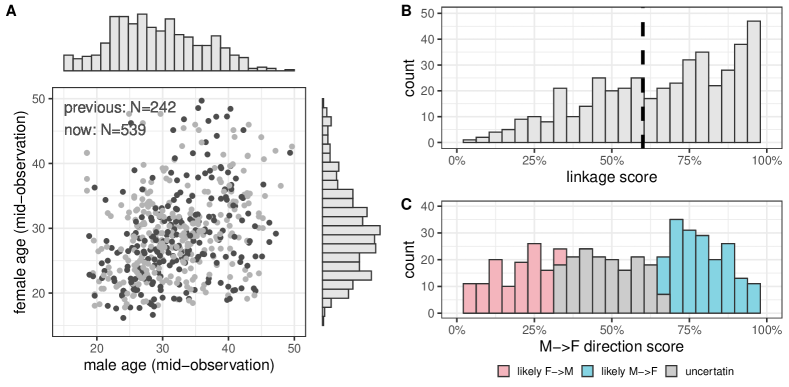
Figure 1: Point data and marks representing the output of HIV phylogenetic deep-sequence analysis on the sequence sample from Rakai, Uganda from 2010 to 2015 . (A) Paired ages of 539 heterosexual individuals who were inferred to be phylogenetically closely related with the HIV phylogenetic deep-sequence analysis using the phyloscanner software on HIV deep-sequence data from 2652 study participants of the Rakai Community Cohort Study in Southern Uganda, 2010 to 2015. The age of the individuals in the closely related pairs was calculated at the midpoint of the observation period, and the age of the men and of the women are shown on the x-axis and y-axis respectively. Each data point is associated with two phylogenetic deep-sequence summary statistics in $[0,1]$, the linkage score ($\ell_{i}$) and the direction score ($d_{i}$) (see text). Points associated with high linkage and direction scores ($\ell_{i}\geq 0.6$ and $d_{i}\geq 0.67$) are shown in dark grey, and all other points are shown in light grey. Marginal histograms on the age of men and women are shown for all points. The typed point process model that we develop here aims to infer transmission flows using all data points rather than the highly likely “source-recipient" pairs shown in dark grey. (B) Histogram of the linkage scores across all data points. (C) Histogram of the direction scores across all data points. Direction scores $d_{i}\leq 1/3$ indicate high confidence in female-to-male transmission (shown in red), and direction scores $d_{i}\geq 2/3$ indicate high confidence in male-to-female transmission (shown in blue).

2.1 Demographic and viral phylogenetic data of HIV infected individuals

HIV deep-sequence data were obtained from blood samples of study participants living with HIV in the Rakai Community Cohort Study (RCCS), a longitudinal, open, population-based census and cohort study in southern Uganda (Grabowski et al., 2017). Samples were collected between August 2011 and January 2015 from 5142 participants (Ratmann et al., 2019), of whom 2652 had an HIV viral load $>1000$ copies/ml and viral sequence read depth and length sufficient for deep sequence data generation and analysis (Wymant et al., 2018; Ratmann et al., 2019). Detailed demographic, behavioural and healthcare data were collected for all participants, including their gender and age, the latter determined from self-reported birth date (Grabowski et al., 2017).

The data that motivate our model consist of a subset of 539 heterosexual pairs of HIV infected RCCS participants considered as phylogenetically likely HIV transmission pairs. These likely transmission pairs were identified based on demographic survey responses about long-term sexual relationships as well as phylogenetic evidence extracted using the phyloscanner deep-sequence analysis pipeline (Wymant et al., 2018). We provide an illustration of the data in Figure 1. There are two main facets of the data. The first facet comprises the age of the two individuals in a pair at the midpoint of the observation period, which we denote by $\mathbb{S}=\{\mathbf{s}_{i}=(a_{i1},a_{i2})^{T}\}_{i=1}^{N}$, where the 2-dimensional vector $(a_{i1},a_{i2})$ records the male’s age $a_{i1}$ and female’s age $a_{i2}$ in the $i$th pair. In our application, the sample size is $N=539$. Our model will envision these points of paired ages as an observation from a spatial process describing the transmission structure. The second facet consists of two scores in the range of $(0,1)$ that are outputs from deep-sequence phylogenetic analyses of HIV deep-sequencing data with phyloscanner. For each pair $i$ of individuals, phyloscanner produces two scores — a linkage score and a direction score — by assessing the viral phylogenetic relationship of individuals in terms of the patristic distances and topological configurations of the viral reads in deep-sequence phylogenies, and then counting the observed patterns over sliding, overlapping genomic windows across the HIV genome (Wymant et al., 2018; Ratmann et al., 2019). The linkage score $\ell_{i}$ represents the posterior probability of the pair sharing a transmission link in the transmission process under a Binomial count model of window-specific linkage classifications (Ratmann et al., 2019). The direction score $d_{i}$, on the other hand, measures the posterior probability of transmission taking place from the male to the female in this pair under a similar count model. We collectively denote the phylogenetic scores for the $i$th pair by $\mathbf{x}_{i}=(\ell_{i},d_{i})^{T}$, and for brevity refer to the phylogenetic data as the “marks" associated with each of the points $\mathbf{s}_{i}$ for $i=1,\dotsc,N$.

The key data challenge is the unobserved transmission relationship between pairs of HIV-infected individuals. Even for a pair with phylogenetic evidence suggesting high probability to be linked through disease transmission (with a high $\ell_{i}$ score), we do not have direct knowledge about the transmission linkage and direction. Our model (described later) will, therefore, probabilistically characterize the likelihoods of pairwise transmission linkage and direction in a data-driven manner.

2.2 Substantial data information loss in existing modeling approaches

Existing analyses attempt to address the unobserved pairwise transmission relationships by pre-classifying data points using heuristic thresholds on the phylogenetic summary scores (Xi et al., 2022; Ratmann et al., 2020; Hall et al., 2021). For example, a potential transmission pair $i$ would be classified to represent a male-to-female transmission event if $\ell_{i}>0.6$ and $d_{i}>0.67$; similarly, another pair $j$ would be taken as a female-to-male transmission if $\ell_{j}>0.6$ and $d_{j}<0.33$ (Xi et al., 2022). Such thresholding a priori, albeit procedurally simple, excludes a substantial proportion of data from the analysis, as “low-confidence” pairs are completely discarded. Graphically, Figure 1 shows that all data points with linkage scores falling to the left of the vertical line in panel B and all data with direction scores in the gray region of panel C would be discarded, resulting in only 242 out of 539 total data points (see panel A) retained for analysis. Further, such pre-classification neglects differential strengths of phylogenetic evidence from data points classified as transmission events. Intuitively, we should have higher confidence about a likely transmission pair $i$ with $\ell_{i}=0.98$ to represent a transmission event, compared to another pair $j$ with only $\ell_{j}=0.61$. However, this difference in evidence strength is not reflected in existing methodology. Instead, all data points that are believed to be “high confidence” pairs are treated as equal and exchangeable, which fails to fully exploit the rich information summarized by the phylogenetic scores. In the next section, we introduce our modeling framework that makes better use of the data by jointly leveraging phylogenetic evidence and demographic information.

2.3 The typed point process model

We now specify a general framework for inferring population-level transmission flows from the point pattern $\mathbb{S}=\{\mathbf{s}_{i}=(a_{i1},a_{i2})^{T}\}_{i=1}^{N}$ with associated marks $\mathbf{x}_{i}=(\ell_{i},d_{i})^{T}$, i. e. the phylogenetic transmission and direction scores. The marks reflect the strength of phylogenetic evidence regarding the unknown ground truth transmission relationship in each heterosexual pair. For this purpose we introduce for each point a categorical latent random variable $c_{i}$ that encodes three possible events: transmission did not occur between the two individuals that define the point (denoted by $c_{i}=0$), transmission occurred from the male to the female individual (denoted by $c_{i}=1$), or transmission occurred from the female to the male individual (denoted by $c_{i}=-1$). For brevity, we refer to the $c_{i}$ as the latent “types" associated with each observed point $\mathbf{s}_{i}$ and observed mark $\mathbf{x}_{i}$. Intuitively, our modelling framework can then be thought of as a typed spatial Poisson process in the sense that the intensity function of the process and the distribution of the marks both depend on the event type, and then the typed process provides a generative model for marked point patterns. This framework, though motivated by our particular application, can be applied to many similar data sets of spatial point patterns of unknown types that are informed by marks associated with each point.

With this context in place, we begin by considering a spatial point pattern defined on a 2-dimensional space $\mathcal{S}\times\mathcal{S}$, where $\mathbb{S}=\{\mathbf{s}_{i}\}_{i=1}^{N}$ is the set of all points, and each point $\mathbf{s}_{i}=(s_{i1},s_{i2})^{T}$ is represented as a point in this plane. We model the observed points in $\mathbb{S}$ as a realization of a 2D Poisson process on $\mathcal{S}\times\mathcal{S}$:

$$\mathbb{S}\sim PP(\boldsymbol{\lambda}).$$ (1)

Following Kottas and Sansó (2007) we decompose the intensity function $\boldsymbol{\lambda}$ into a scale component $\gamma$ and a density function $f(\cdot)$,

$$\boldsymbol{\lambda}(\cdot)=\gamma f(\cdot),$$ (2)

so that $f(\cdot)$ satisfies $\int_{\mathcal{S}\times\mathcal{S}}f(s_{1},s_{2})ds_{1}ds_{2}=1$. This decomposition separates the intensity function into two terms which are simpler to write out in the likelihood function and make inference computationally tractable. We next model the density function $f(\cdot)$ as a mixture of $K$ different types:

$$f(\cdot)=\sum_{k\in\mathcal{K}}p_{k}f_{k}(\cdot),$$ (3)

where $p_{k}$ is the probability of points belonging to type $k$, and $f_{k}(\cdot)$ is the spatial density function for type $k$. In the context of our application, $\mathcal{S}$ is the continuous age of individuals under study, $\mathcal{S}=[15,50)$. Each point $\mathbf{s}_{i}=(a_{i1},a_{i2})^{T}$ corresponds to the ages of the two individuals forming a pair, ordered by gender and the latent types are $\mathcal{K}=\{-1,0,1\}$, corresponding to female-to-male transmission, no transmission and male-to-female transmission. For instance $p_{1}$ corresponds to the proportion of male-to-female transmission events among all pairs of individuals being considered, and $f_{1}(\cdot)$ corresponds to the 2D function that captures the across-age transmission pattern with male sources and female recipients.

2.4 Infinite Gaussian mixture models for the typed intensity functions

There are various choices to model the structure of the density functions $f_{k}(\cdot)$. To balance simplicity and flexibility, we choose a Dirichlet process (“DP”) Gaussian mixture model (“DPGMM”) consisting of infinitely many bivariate Gaussian components $f_{k}(\cdot)$. Specifically, for each point $\mathbf{s}_{i}$, if its type label $c_{i}=k$, then

$$\mathbf{s}_{i}\mid c_{i}=k\sim N(\theta_{ki},\Sigma_{ki}),\quad(\theta_{ki},\Sigma_{ki})\sim G_{k},\quad G_{k}\sim DP(\alpha_{k},G_{0}).$$ (4)

Here $G_{k}$ represents the (infinite) mixture of bivariate normal models for type $k$, and $\theta_{ki}$ and $\Sigma_{ki}$ are the mean vector and covariance matrix for the bivariate Gaussian component that $\mathbf{s}_{i}$ belongs to. In practice, Dirichlet process mixtures are often treated as a finite mixture but with a flexible number of components. Indeed, the above defined model may be expressed equivalently in terms of each density function $f_{k}(\cdot)$,

$$f_{k}(\cdot)=\sum_{h=1}^{H_{k}}w_{kh}\cdot\text{dBVN}(\cdot;\theta_{kh},\Sigma_{kh}),$$ (5)

where $H_{k}$ denotes the number of “active” components, or total number of unique components generated by the DP, and each $(\theta_{kh},\Sigma_{kh})$ is a unique Gaussian component for the type-$k$ density. Here, $\text{dBVN}((s_{1},s_{2});\theta,\Sigma)$ denotes the probability density of a bivariate normal distribution with mean $\theta$ and covariance $\Sigma$.

2.5 Model for type-dependent marks

We next describe how the observed point patterns and the associated marks are connected under the typed point process model. We presume that the marks $\mathbf{x}_{i}$ associated with each point $\mathbf{s}_{i}$ should provide information on the true event type $c_{i}$ of each point. This prompts us to model the distribution of the marks conditional on the event type. In our application the marks $\mathbf{x}_{i}=(\ell_{i},d_{i})^{T}$ are two dimensional vectors with entries taking values in $(0,1)$, and we assume the following type-dependent distribution for $\mathbf{x}_{i}$ conditional on the type value $c_{i}=k$ ($k\in\{-1,0,1\}$):

$$p(\mathbf{x}_{i}\mid c_{i}=k)=\phi_{k}((\ell_{i},d_{i})^{T})=dN(\text{logit}(\ell_{i});\tilde{\mu}_{\ell,i}(k),\sigma_{\ell}^{2})\times dN(\text{logit}(d_{i});\tilde{\mu}_{d,i}(k),\sigma_{d}^{2}).$$ (6)

Here, $dN(\cdot;\mu,\sigma^{2})$ denotes a univariate normal density function with mean $\mu$ and variance $\sigma^{2}$, and $\text{logit}(x)$ denotes the logit transformation on $x\in(0,1)$. We further specify type-dependent normal means $\tilde{\mu}_{\ell,i}(k)$ and $\tilde{\mu}_{d,i}(k)$:

$$\tilde{\mu}_{\ell,i}(k) =\mu_{\ell}\mathbbm{1}\left[k\neq 0\right],$$ (7)

$$\tilde{\mu}_{d,i}(k) =\mu_{d}\mathbbm{1}\left[k=1\right]+\mu_{-d}\mathbbm{1}\left[k=-1\right].$$ (8)

Intuitively, a larger linkage score $\ell_{i}$ indicates stronger evidence for a transmission event, and a larger direction $d_{i}$ indicates higher confidence for a male-to-female transmission. Thus, with $\mu_{\ell}>0$, (7) implies that the linkage score $\ell_{i}$ is likely to exceed $0.5$ for a real transmission event ($c_{i}\neq 0$); similarly, with $\mu_{-d}<0<\mu_{d}$, (8) implies that $d_{i}$ is likely larger than $0.5$ for a male-to-female event ($c_{i}=1$) but smaller than $0.5$ for a female-to-male event ($c_{i}=-1$). Note that such design uses the property $\text{logit}(0.5)=0$.

2.6 The complete data likelihood

From the descriptions in the previous section, we see that the two key components in the model—the spatial process and the marks distribution —are linked through the latent types $c_{i}$. Conditional on the latent type $c_{i}=k$, a point $i$ contributes the term $\gamma p_{k}f_{k}(\mathbf{s}_{i})\times\phi_{k}(\mathbf{x}_{i})$ to the data likelihood, and therefore the likelihood is merely a product of all such terms for $i=1,2,\ldots,N$. Thus, we first construct the likelihood function given the “complete” data, which include the coordinates of all $N$ points in the set $\mathbb{S}$, the observed signals $\mathbf{x}_{i}$ as well as the type $c_{i}$ for all $i=1,\ldots,N$. We have essentially derived all components in the exposition above, comprising the expression

$$L(\Theta;\{\mathbf{x}_{i}\},\{c_{i}\},\{\mathbf{s}_{i}\}) =\gamma^{N}\frac{e^{-\gamma}}{N!}\prod_{k\in\mathcal{K}}\prod_{i:c_{i}=k}p_{k}f_{k}(\mathbf{s}_{i})\phi_{k}(\mathbf{x}_{i})$$ (9)

$$= \prod_{i=1:N}dN(\text{logit}(\ell_{i});\tilde{\mu}_{\ell,i}(c_{i}),\sigma_{\ell}^{2})dN(\text{logit}(d_{i});\tilde{\mu}_{d,i}(c_{i}),\sigma_{d}^{2})$$ (10)

$$\times\gamma^{N}\frac{e^{-\gamma}}{N!}\prod_{k\in\mathcal{K}}\prod_{i:c_{i}=k}\left(p_{k}\sum_{h=1}^{H_{k}}w_{kh}\text{BVN}((s_{i1},s_{i2});\theta_{h},\Sigma_{h})\right).$$

Here, the model parameters are $\Theta=\{\gamma,\mathbf{p},\boldsymbol{\mu},\sigma_{\ell}^{2},\sigma_{d}^{2},\{(\theta_{kh},\Sigma_{kh})\},\{\alpha_{k}\}\}$, where we further abbreviate $\mathbf{p}=(p_{-1},p_{0},p_{1})^{T}$, and $\boldsymbol{\mu}=(\mu_{\ell},\mu_{d},\mu_{-d})^{T}$).

3 Bayesian inference with data augmentation

We employ an efficient data-augmented Bayesian inference scheme to learn the unknown parameters $\Theta$ in the proposed typed point process model from observed data. Inference would be straightforward if all aspects of the model were observable, giving access to the complete data likelihood specified in (10). That is, if the $c_{i}$’s were known, the terms corresponding to the spatial point process and marks completely factorize in the likelihood function, as shown in (10). Parameter inference would reduce to standard procedures for Dirichlet Process Gaussian mixture models (Rasmussen, 1999).

However, the types $c_{i}$ for each data point $i$ are not observed in our data setting. Because it is not clear whether direct marginalization is possible, we propose a data augmentation inference scheme that expands the target posterior to include the unobserved $c_{i}$’s as unknowns. Conditioning on a given setting of their values then gives us access to the tractable complete data likelihood function. That is, our algorithm samples from the joint posterior density of the model parameters $\Theta$ together with the unobserved types $c_{i}$’s:

$$p(\Theta,\{c_{i}\}\mid\{\mathbf{x}_{i}\},\{\mathbf{s}_{i}\}) \propto L(\Theta;\{\mathbf{x}_{i}\},\{c_{i}\},\{\mathbf{s}_{i}\})p_{0}(\Theta).$$ (11)

Here $p_{0}(\Theta)$ denotes the joint prior distribution for parameters $\Theta$, which we will detail in the sequel. The data-augmented inference framework is employed through a Bayesian Markov chain Monte Carlo (MCMC) sampler, which can be roughly divided into two major components in each iteration: (1) sample or update parameters $\Theta$ conditioned on configurations of the $\{c_{i}\}$’s from the conditional posterior distribution $p(\Theta\mid\{\mathbf{x}_{i}\},\{c_{i}\},\{\mathbf{s}_{i}\})$; and (2) sample $c_{i}$ for each $i$ given values of $\Theta$ from $p(c_{i}\mid\Theta,\mathbf{x}_{i},\mathbf{s}_{i})$, utilizing the complete data likelihood in (10). To improve efficiency of the MCMC sampler, we prescribe conjugate or semi-conjugate priors whenever possible, enabling straightforward Gibbs sampling by exploiting full conditional posterior densities available for almost all parameters. Below, we detail these prior choices and discuss each step of the MCMC sampler. A pseudocode summary of our sampler appears as Algorithm 1 in Web Appendix A.

3.1 Scale parameter $\gamma$

Due to the scale decomposition in (2), sampling the parameter $\gamma$ is straightforward and can in fact be done independently of the Markov chain that samples the remaining parameters. That is, if we assign a Gamma prior $\gamma\sim Ga(a_{0},b_{0})$, we may directly draw samples using

$$\gamma\mid{\{\mathbf{x_{i}}\},\{\mathbf{s_{i}}\}}\sim Ga(\alpha_{0}+N,\beta_{0}+1).$$

3.2 Mark distribution parameters $\boldsymbol{\mu}$, $\sigma_{\ell}^{2}$, and $\sigma_{d}^{2}$

Conditioned on type labels $\{c_{i}\}$, the signal distributions for $\ell_{i}$’s and $d_{i}$’s (6) are simple univariate normal models. Assuming diffuse priors $\mu_{\ell},\mu_{d}\sim\text{Unif}((0,\infty))$, $\mu_{-d}\sim\text{Unif}((-\infty,0))$ and inverse-Gamma priors $\,\sigma_{\ell}^{2},\sigma_{d}^{2}\sim\text{inv-Gamma}(\nu_{0}/2,\nu_{0}\sigma_{0}^{2}/2)$  , parameter updates only require straightforward Gibbs steps from the full conditionals. For example, for the linkage score parameters $\mu_{\ell}$ and $\sigma^{2}_{\ell}$, we draw

$$\mu_{\ell}\mid\sigma^{2}_{\ell},\{\ell_{i}\},\{c_{i}\} \sim N_{(0,\infty)}\left(\sum_{i:c_{i}\neq 0}\text{logit}(\ell_{i}),\sigma^{2}_{\ell}/N_{+}\right)$$

$$\sigma^{2}_{\ell}\mid\mu_{\ell},\{\ell_{i}\},\{c_{i}\} \sim\text{inv-Gamma}\left(\frac{\nu_{0}+N_{+}}{2},\frac{\nu_{0}\sigma_{0}^{2}+\sum_{i:c_{i}\neq 0}(\text{logit}(\ell_{i})-\mu_{\ell})^{2}}{2}\right).$$

Here $N_{+}=\sum_{i=1}^{N}\mathbbm{1}(c_{i}\neq 0)$ is the total number of real transmissions given the $\{c_{i}\}$ configurations, and $N_{(0,\infty)}$ denotes a normal distribution truncated on the positive real line. For the direction score parameters $\mu_{d},\mu_{-d}$ and $\sigma_{d}^{2}$, sampling steps are almost completely analogous.

3.3 Type probabilities $\mathbf{p}$

Assuming a Dirichlet prior for the probability vector $\mathbf{p}=(p_{-1},p_{0},p_{1})$, $\mathbf{p}\sim\text{Dir}(q_{-1},q_{0},q_{1})^{T}$ and given configurations for $\{c_{i}\}$, we can draw

$$\mathbf{p}\mid\{c_{i}\}\sim Dir\left(q_{-1}+N_{-1},q_{0}+N_{0},q_{1}+N_{1}\right),$$

where $N_{k}=\sum_{i=1}^{N}\mathbbm{1}(c_{i}=k)$ is the total number of data points belonging to type $k$.

3.4 DP precision parameter $\alpha_{k}$ and component weights $w_{kh}$

For the precision parameter $\alpha_{k}$ and weights $w_{kh}$ for each type $k$, we adopt a truncated DP mixture model with a large maximum number of mixtures to approximate the infinite DP mixture, a technique described in Section 3.2 and in the Appendix of Ji et al. (2009). More specifically, we use an auxiliary sampling trick introduced in Escobar and West (1995) to update the precision parameter $\alpha_{k}$’s for $k=0,-1,1$). By introducing an additional auxiliary parameter to sample along with each $\alpha_{k}$, the conditional posterior distribution for $\alpha_{k}$ can be reduced to a mixture of two Gamma distributions, which conveniently transforms its sampling step to a simple Gibbs step. For complete technical details, we refer the reader to Ji et al. (2009) and Escobar and West (1995).

3.5 BVN mixture components $(\theta_{kh},\Sigma_{kh})$

For the bivariate normal mixture model of each type $k$, we introduce a component latent indicator $z_{i}$ for each data point $i$ (that belongs to type $k$) such that $z_{i}=h$ indicates point $i$ belongs to component $h$. Assuming semi-conjugate priors $\theta_{kh}\sim\text{BVN}(\theta_{0},\Sigma_{0})$ and $\Sigma_{kh}\sim\text{inv-Wishart}(\nu,S_{0})$, we then iteratively update the $z_{i}$’s and $(\theta_{kh},\Sigma_{kh})$’s using

$$Pr(z_{i}=h\mid w_{kh},\theta_{kh},\Sigma_{kh},\mathbf{s_{i}}) \propto w_{kh}\cdot\text{dBVN}(\mathbf{s}_{i}\mid\theta_{kh},\Sigma_{kh})$$

$$\theta_{kh}\mid\Sigma_{kh},\{z_{i}\},\{\mathbf{s_{i}}\} \sim\text{BVN}\bigg{(}(m_{h}\Sigma_{kh}^{-1}+\Sigma_{0}^{-1})^{-1}\left(\sum_{i:z_{i}=h}\Sigma_{kh}^{-1}\mathbf{s_{i}}+\theta_{0}\Sigma_{0}^{-1}\theta_{0}\right),$$

$$\quad\quad\quad\quad\quad(m_{h}\Sigma_{kh}^{-1}+\Sigma_{0}^{-1})^{-1}\bigg{)};$$

$$\Sigma_{kh}\mid\theta_{kh},\{z_{i}\},\{\mathbf{s_{i}}\} \sim\text{inv-Wishart}\left(\nu+m_{h},\left(S_{0}^{-1}+\sum_{i:z_{i}=h}(\mathbf{s_{i}}-\theta_{kh})(\mathbf{s_{i}}-\theta_{kh})^{T}\right)^{-1}\right).$$

Here $\text{dBVN}(\cdot\mid\theta,\Sigma)$ is the density function of a bivariate normal with mean $\theta$ and covariance matrix $\Sigma$, and $m_{h}=\sum_{i=1}^{N}\mathbbm{1}(z_{i}=h)$ is the total number of data points belonging to spatial component $h$.

3.6 Type indicators $c_{i}$

The type $c_{i}$ can be sampled for each data point $i$ conditioned on all other parameter values and the observed data via its full conditional distribution $Pr(c_{i}=k\mid\Theta,\mathbf{s}_{i},\mathbf{x}_{i})\propto p_{k}f_{k}(\mathbf{s}_{i})\phi_{k}(\mathbf{x}_{i})$.

4 Simulation studies

In this section, we validate the modelling and inference framework for marked point patterns through synthetic experiments. With our application in mind, we focus on assessing whether the typed point process model can accurately recover simulated patterns of HIV transmission flows between men and women across different ages. We further explore the ability of the model to infer these flows at increasingly smaller sample sizes. Throughout this section, we focus on two contemporary questions of particular epidemiological interest, and investigate the ability of the typed point process model in recovering and differentiating between two competing scenarios.

First, one general finding of recent HIV transmission flow studies is that there tend to be more infections that originate from men than from women (Hall et al., 2021; Bbosa et al., 2020; Ratmann et al., 2020). This prompts us to explore whether the typed point process model can accurately recover parameters and distinguish between a scenario in which men drive 50% of infections (“MF-50-50") and a scenario in which men drive 60% of infections (“MF-60-40”). We explore $5$ different sample sizes (i.e., numbers of likely transmission pairs) with $N=100,200,400,600$ and $800$. For each scenario and each sample size, $100$ independent data sets were generated, and the typed point process model fitted to each. Details on the simulations and scenarios are fully described in Web Appendix B.

Second, there is broad interest in the age distribution of the male sources of HIV infections, especially for adolescent girls and young women aged 15 to 24, due to the high incidence rates in these women (Risher et al., 2021). This prompts us to investigate if the model can distinguish between two scenarios in which either younger men of approximately 25 years (within $\pm 5$ years age difference of adolescent and young women) contribute 60% to infections in women aged 15-24 years and older men of approximately 35 years 30%, and other men 10% (“SAME AGE"); versus the alternative scenario that younger men of approximately 25 years contribute 30%, and older men of approximately 35 years 60%, and other men 10% (“DISCORDANT AGE"). We varied the sample sizes, generated simulations and fitted the model as before, with complete details described in Web Appendix B.

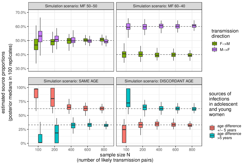
Figure 2: Performance of the typed point process model in recovering simulated transmission flow patterns. Inference using the typed point process model was performed on each of the 100 simulated data sets for each scenario. A Boxplot of the posterior mean estimate of transmissions from men in 100 replicate simulations for the MF-50-50 (left panel) and MF-60-40 scenarios (right panel). Throughout, the dashed lines mark the true values that underpin the simulated data. The x-axis shows the sample size of simulated data points, which represent the number of phylogenetically closely related pairs of individuals identified through phylogenetic deep-sequence analyses. B Boxplot of the posterior mean estimate of transmissions from men of similar age (shown in red) and older age (shown in blue) to infection in adolescent and young women aged 15-24 in 100 replicate simulations for the “SAME AGE” and “DISCORDANT AGE” scenarios. As before the dashed lines mark the true values that underpin the simulated data and the x-axis shows results for different sample sizes.

Figure 2 (top panel) summarizes our findings on the male-female simulation experiments (MF-50-50 and MF-60-40). Our findings reveal that the model is able to successfully distinguish between the two competing epidemiological scenarios with sample size $N\geq 200$, and produces estimates that are accurate within a $\pm 5$% error margin for sample sizes $N\geq 200$. Figure 2 (bottom panel) illustrates our findings on the age-specific sources experiments (SAME-AGE, DISCORDANT-AGE). This is a substantially more difficult inference problem because the target quantities relate to a smaller subgroup of the entire source population. With a small sample ($N$ in the range $100-200$), the relative relationship between the two proportions is inferred correctly in all experiments. However, the actual quantitative estimates and differences can be far from the truth, and tend to be over-estimated. For sample sizes of $N\geq 400$, the quantitative estimates become accurate for practical purposes. The observed over-estimation is likely due to the parsimony induced by the Dirichlet Process priors that are known to prefer assigning data points to the largest existing clusters when there are not enough data to admit a new mixture model component. As a result, more points tend to be attributed to the component with the highest weight when $N$ is small; this effect is mitigated as $N$ increases. Additional analyses on simulated experiments are included in Web Appendix B. These include numerical convergence and mixing analyses, which are generally quite satisfactory, as well as Bayesian coverage analyses, which indicate that the posterior distributions of the target quantities are well calibrated.

5 Case study

We are now ready to apply the typed point process model to study demographic and population-based HIV deep-sequence data collected from the Rakai Community Cohort Study in Southeastern Uganda between August 2011 and January 2015 (Ratmann et al., 2019, 2020; Xi et al., 2022). Our aim is to reconstruct transmission flows by gender and continuous age between 15 and 50 years. This case study is challenging in the sense that phylodynamic analyses using standard HIV consensus sequences have difficulty inferring flow patterns for more than a handful of age groups: many contemporary analyses of age-specific transmission flows remain limited to a resolution of 5-year or 10-year age bands (Scire et al., 2020; Bbosa et al., 2020; Le Vu et al., 2019; De Oliveira et al., 2017; Ratmann et al., 2020).

We revisit the HIV deep-sequence dataset considered by  Xi et al. (2022), and compare our approach applied to the complete dataset without appealing to heuristic pre-classification that results in utilizing only a small subset of data. More specifically, we will use the typed point process model to analyze all pairs of closely phylogenetically related individuals introduced in Section 2. After filtering out only pairs of individuals with a linkage score $<0.2$ (i.e., pairs with very weak evidence), we retain a dataset of 526 pairs that represent potential transmission events. For comparison purposes, we also repeat the analysis under the heuristic thresholding approach following Xi et al. (2022); this pre-processing step retains only retains a subset of those pairs of individuals as “high-confidence” transmission pairs. Referring to the first as the “full analysis with latent event types” (or “full analysis” in short), we fit the typed point process model to all data, simultaneously inferring the three latent event types in our application, $k=0$ for no transmission event, $k=1$ representing male-to-female transmission, and $k=-1$ for female-to-male transmission (recall the Methods section). In the second “subset analysis with fixed event types” (“subset analysis” in short), we retain similarly as in (Xi et al., 2022; Hall et al., 2021) only those data with linkage scores $>0.6$ and a direction score $>0.5$ as a male-to-female transmission pair, and those with linkage scores $>0.6$ and a direction score $\leq 0.5$ as a female-to-male transmission pair. In the full analysis, all 526 data points will be used, while the subset analysis considers only 367 pairs. This is a larger subset of data retained compared to Xi et al. (2022) which consists of 238 pairs of individuals, where only “high-confidence” potential transmission pairs with direction score $<0.33$ or $>0.67$ were retained for analysis. In both analyses, we adopt the same priors as described in Section 4 and run the MCMC algorithm detailed in Section 3 for 3000 iterations after 1000 burn-in steps.

5.1 Learning the latent event types is computationally feasible

We are able to infer both the transmission flow surfaces of interest, $f_{1}$ and $f_{-1}$ in (3), and the unknown event types $\{c_{i};i=1,\dotsc,N\}$ for each observed data point without issues in numerical convergence or mixing. On a laptop with a 4-core Intel CPU, the full analysis with the typed point process model including the latent event types takes less than 10 minutes, which is a considerable improvement in computational efficiency compared to using the semi-parametric Poisson count model on 1-year age discretized bands Xi et al. (2022), where 4000 total iterations requires about 30 hours. This speed-up is expected, as our typed point process model greatly simplifies computation through a continuous spatial point pattern specification that only requires likelihood evaluations on the observed $526$ data points. In comparison, the Poisson count model in Xi et al. (2022) involves likelihood evaluations on all $2\times(50-15)^{2}=2450$ grid cells, many of which contain structural zeros.

5.2 Learning latent event types results in more data used for inference of transmission flows

In comparison to the subset analysis, the full analysis appears to attribute more pairs of individuals to type $1$ (male-to-female transmission) and to type $-1$ (female-to-male transmission). We present the posterior probability $p_{k}$ for each type as inferred by the full analysis and by the subset analysis in Table 1. Multiplying the estimated $p_{k}$’s by sample size $526$, we also calculate the number of pairs, $N_{k}$, that each analysis has attributed to each type. Notably, the full analysis learns a $p_{0}$ (proportion of “no transmission”) that is significantly lower than that under the fixed event type subset analysis. This indicates that, by probabilistically inferring event types instead of heuristically pre-classifying them, our proposed approach is utilizing more phylogenetically close pairs to learn the transmission flows. In short, our approach not only reflects uncertainty in event types, but also makes more efficient use of phylogenetic and demographic evidence in data.

Table 1: Proportions and numbers of inferred event types. Posterior mean estimates with 95% credible intervals.

Type	Full analysis		Subset analysis
	with latent event types		with fixed event types
	$p_{k}$	$N_{k}$	$p_{k}$	$N_{k}$
Male-to-Female	46.3% (39.4%, 53.1%)	244 (207, 279)	35.7%	188
transmission $(k=1)$
Female-to-male	35.0% (28.5%, 42.0%)	184 (150, 221)	29.5%	155
transmission $(k=-1)$
No transmission	18.6% (9.4%, 29.2%)	98 (49, 154)	34.8%	183
$(k=0)$

5.3 Inferred age of male and female sources of HIV transmission.

With the typed point process model, we are able to estimate the sources of male and female HIV infection events in terms of the continuous age of the sources (Figure 3(a)). This is an important advantage over other approaches through which the age of the sources can be characterised by 5-year or 10-year age bands (Scire et al., 2020; Bbosa et al., 2020; Le Vu et al., 2019; De Oliveira et al., 2017), because at such coarse scale discretization introduces artifacts that obfuscate differences in transmission modes that are important to differentiate from a public health perspective (Xi et al., 2022). Figure 3(a) addresses the following question about HIV transmission — which age groups contribute most to HIV transmission at the population-level? The colored solid curves and text illustrate the inferred age distribution of the male and female sources in the full analysis with latent event types, while the dark dashed lines and dark text summarize results for the subset analysis with fixed event types. We find that the inferred age distribution of the male and female sources are very similar in both analyses.

More specifically, during the observation period 2011-2015, male sources tended to be consistently older than female sources. The estimated 50% highest posterior density intervals (HDIs) learned in the full analysis with latent event types are ages $[25.4,34.3]$ for male sources and ages $[20.4,29.0]$ for female sources. In comparison, the 50% posterior HDI inferred in the subset analysis with fixed event types are $[26.9,35.4]$ for the age distribution of male sources, and $[21.4,29.3]$ for female sources. This indicates that estimation uncertainty in quantities of key epidemiological interest did not decrease in the full analysis. Rather, we find that the full analysis using latent event types better reflects the actual uncertainty in key quantities, as the typed point process model explicitly accounts for uncertainty in the event types that underpin each data point.

Both the full and the subset analyses indicate a characteristic peak in transmission from men around 30 years of age, and a long, pronounced tail of transmissions from older men beyond age 40. In this regard, we find that the age distribution of the female sources differs qualitatively, as the probability of transmissions from women declines more rapidly with age, reaching similar levels by age 30 in women compared to age 45 in men. In the full analysis with latent event types, these observations on the age of the female sources are more strongly supported, as in the full analysis the entire age distribution of the female sources is slightly shifted towards younger ages compared to the age distribution of the female sources in the subset analysis with fixed event types.

We can gain further insight into age-specific transmission dynamics by considering the age profile of the transmitting partners for recipients of a particular age. In Figure 4, the age of a recipient is shown in colour, and the wave on the $y$-axis shows the posterior median contribution of transmissions to recipients of the age indicated in colour. Figure 4(a) illustrates that the age profile of sources has a characteristic shape for each recipient age group, and in particular are not simply shifted versions of one age profile. Figure 4(b) demonstrates how the superposition of the age-structured transmission dynamics results in the overall source profile that marginalises out the age of the recipients.

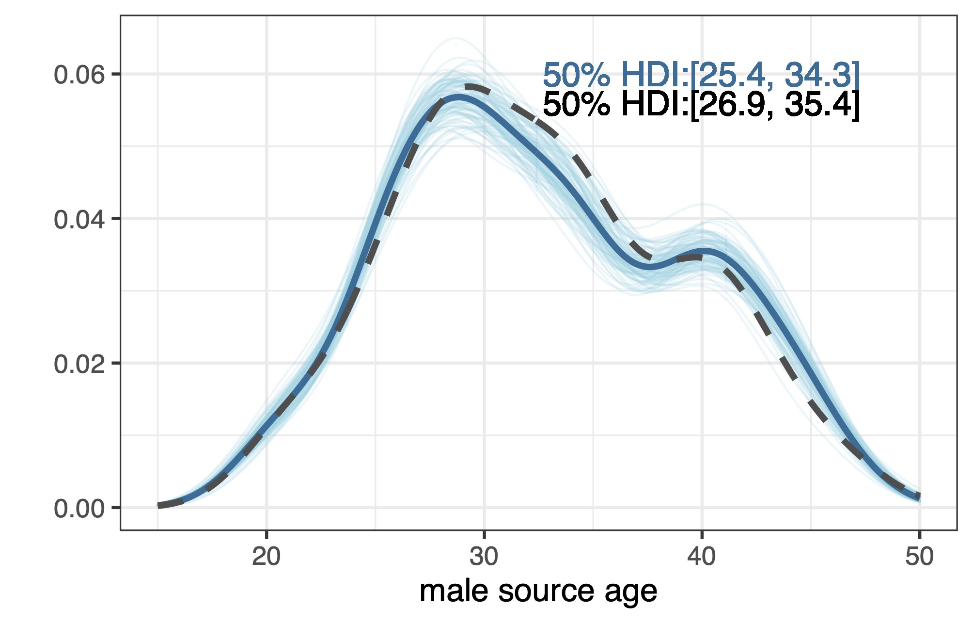
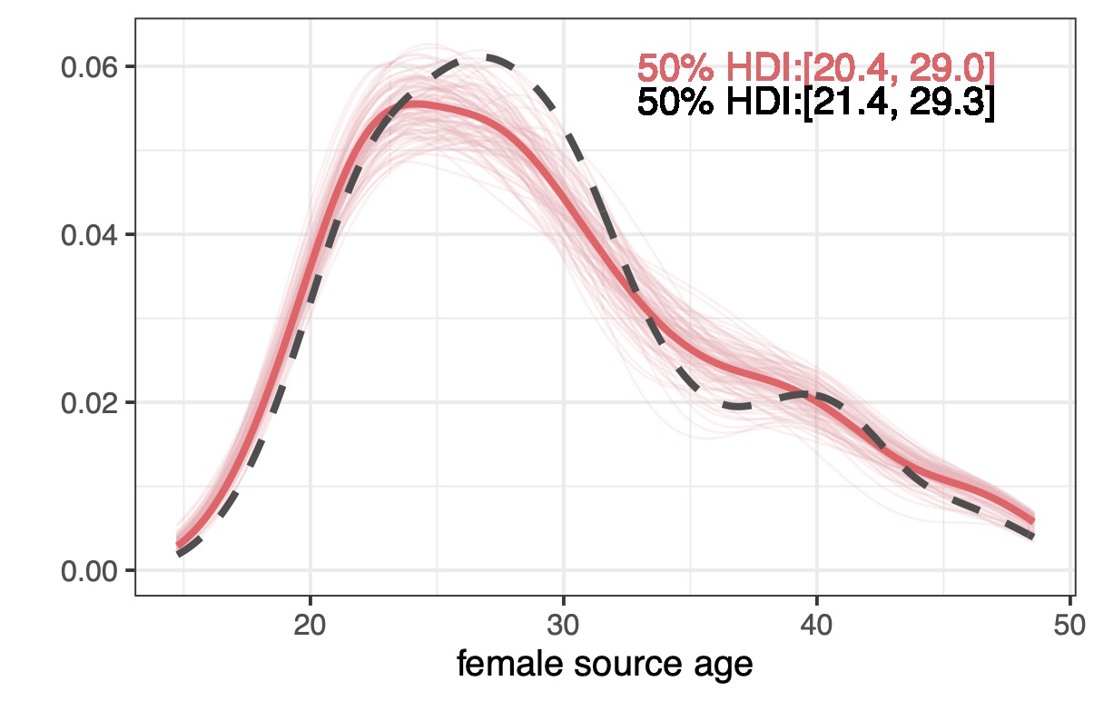
(a) Age distributions of male and female sources of HIV infections in Rakai, Uganda during the 2011-2015 observation period. The left panel shows the estimated age of the male sources and the right panel the estimated age of the female sources.

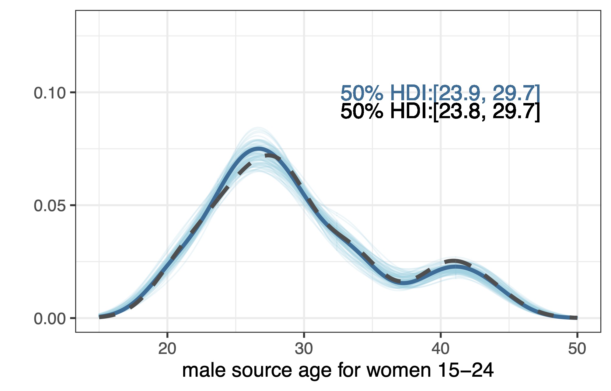
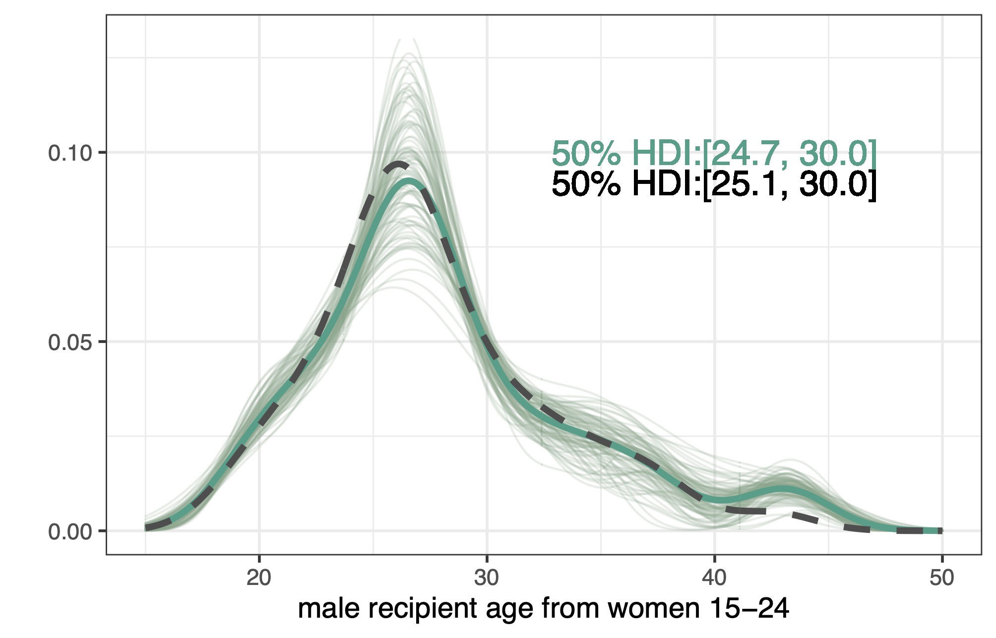
(b) Age distributions of male sources and recipients of HIV infections in women aged 15-24. Left panel shows the age distribution of male sources, and right panel characterizes age distribution of male recipients, for women aged 15-24.

Figure 3: Age distributions of sources and recipients, for the general population (subplot 3(a)) and for women aged 15-24 (subplot 3(b)). In each panel, the colored lines represent density curves of the age of sources/recipients for 100 posterior samples from the inferred, smooth transmission flow intensity surface of the typed point process model in the full analysis with latent event types. The thicker curve indicates the posterior mean density curve. The black dashed curve illustrates the posterior mean density curve in the subset analysis with fixed event types. 50% highest density intervals (HDIs) are marked in text, with colored text indicating the HDIs inferred in the full analysis and black text indicating the HDIs inferred in the subset analysis.

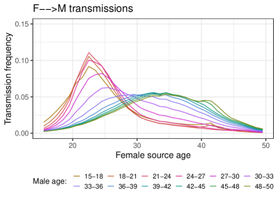
(a) Age distributions of sources for recipients in different 3-year age groups. Each curve represents the learned relative frequencies of sources responsible for transmissions within each recipient age group.

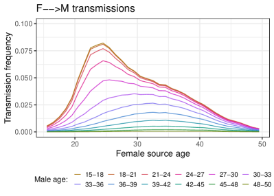
(b) Marginal age distributions of sources. Shown as “stacked” curves of age source distributions for each recipient age group (in 3-year age bands).

Figure 4: Age distributions of sources for heterosexual recipients in different age groups (by 3-year age bands). In subplot 4(a), the curves for each recipient age group represent posterior means of the source age distributions learned by the full analysis with latent event types. In subplot 4(b), the “marginal” age distributions are shown by stacking up the frequencies of sources for each recipient age group. Left column shows age distributions for male sources in male-to-female transmissions for different female recipient age groups. Right column shows age distributions for female sources in female-to-male transmissions for different male recipient age groups.

5.4 Transmissions to and from adolescent and young women

Next, we focus our attention on adolescent and young women of age 15 to 24 years. Specifically, we wish to understand the age distribution of male sources in their infectious, and in turn, that of male recipients for whom these women are the sources of infection. Our rationale is that understanding the age distribution of the male sources and recipients in adolescent and young women can provide further evidence to HIV programs that aim to reduce infections in this age group (Glynn et al., 2001; Pettifor et al., 2008; Karim et al., 2010; Jewkes et al., 2010). One prominent program is the “Determined, Resilient, Empowered, AIDS-free, Mentored, and Safe” (DREAMS) program (Saul et al., 2018) within the US President’s Emergency Plan for AIDS Relief (PEPFAR) Oliver (2012).

Figure 3(b) illustrates the inferred age distributions of the male sources of infections in adolescent and young women (left), and of the male recipients of transmissions from these women (right) in the full analysis with latent event types (colored curves) and the subset analysis with fixed event types (black curves). While the majority of male sources are men between 24 to 30 years, there is also a notable subgroup of male sources older than 35. In contrast, the male recipients of transmission from adolescent and young women lie more strongly in men aged 24 to 30 years, with a much smaller subgroup of male recipients older than 35. That is, a transmission pathway strongly supported by the 2011-2015 data may begin with transmission from men approximately 5-8 years older than adolescent and young women, and who then in turn transmit the virus in smaller numbers to men who are again 5-8 years older than themselves. In addition, a second transmission pathway may begin with transmission from men 10-15 years older than adolescent and young women, and who then in turn transmit the virus in smaller numbers to men who are more likely to be 5-8 years older than themselves, rather than 10-15 years older. Our findings for the 2011-2015 observation period thus further corroborate the importance of major HIV prevention programs across Sub-Saharan Africa that have been directing educational and healthcare resources to adolescent and young women, who are especially vulnerable to HIV from a broad age spectrum of male sources (Saul et al., 2018; UNAIDS, 2018).

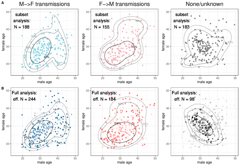
Figure 5: Comparison of the inferred age structure in transmission flows in the full with latent event types versus the subset analysis with fixed event types. (A) Results in the subset analysis with fixed event types. Source-recipient pairs that were pre-classified by event type (dots) are shown along the posterior median estimate of 50%, 80% and 90% highest probability regions of transmission flows (contours). The number of data points attributed to each type is indicated in the top left corner. (B) Results in the full analysis with latent event types. Source-recipient pairs (dots) are shown by posterior event type probabilities (colour intensity) along the posterior median estimate of 50%, 80% and 90% highest probability regions of transmission flows (contours). The “effective” number of data points attributed to each type (posterior mean estimate of $N_{k}$ as in Table 1) is indicated in the top left corner.

5.5 In-depth comparison of the full analysis with latent event types with the subset analysis with fixed event types

We close by examining the more detailed features of the inferred age- and gender-specific transmission flows in the subset analysis with fixed event types (Figure 5A) compared to the full analysis with latent event types (Figure 5B). In the subset analysis with fixed event types, only a subset of all data points are utilized to learn the latent age structure associated with each type, and all data points are assumed to carry the same weight (as colored by the same shade in each panel). In the full analysis with latent event types, all data points contribute to the learning of the latent age structure associated with each event type, and the contribution of each data point is weighted by the posterior event type probabilities associated with each point (as illustrated with the colour shades of each point). Overall, we find that the learned 2D surfaces of age-specific male-to-female transmission flows and female-to-male transmission flows are very similar in the full analysis with latent event types compared to the subset analysis (contours in Figure 5. This is already indicated by the findings on the marginal age distribution of the male and female sources of infection in Figure 3(a).

However, the inferred latent surface corresponding to no transmission differs substantively between the full and subset analyses, with noticeably more data points in the corners of the compact space attributed to either male-to-female or female-to-male transmission. Data points corresponding to combinations of women around age 20 and men around age 30 are more strongly attributed to male-to-female transmission in the full analysis, in line with the strong center of mass of the inferred male-to-female transmission surface for these age combinations. Data points involving women around age 45 are more strongly attributed to female-to-male transmission, in line with the wider tails of the inferred female-to-male transmission surface for these age combinations. This latter observation illustrates the potential limitations of the typed point process model, because women in this age group tend to have lower HIV viral load at the population-level than men, rendering this population group of women on average less infectious than men (Grabowski et al., 2017; Rodger et al., 2019). Within the proposed Bayesian framework, such information could straightforwardly be included by using more informative priors than we have imposed here, which may play an important role for future applications of the typed point process model.

6 Discussion

In this paper, we develop a hierarchical typed point process to learn disease transmission flows from phylogenetically reconstructed transmission pair data. The model is developed alongside a computationally efficient Bayesian sampler targeting the exact likelihood of the specified model. We demonstrate that our novel approach can probabilistically learn the unobserved event types — whether or not there is transmission between a pair and in which direction the transmission occurs — despite the large number of additional latent parameters and partially informative data. Its ability to do so is in large part owing to reformulating the inference problem in terms of a continuous spatial process. Unlike previous work (Xi et al., 2022), this does not require discretization of the feature space and thus avoids keeping track of all cells in a large transmission flow matrix in computation; our method only needs to track all the data points. This advantage by construction renders our approach much more computationally efficient. In simulations and a case study on population-level HIV deep-sequence data from the Rakai Community Cohort Study in Southern Uganda, we demonstrate that the typed point process model allows inclusion of more data in analysis while accounting for the intrinsic uncertainties associated with outcomes of deep-sequence phylogenetic analyses. The primary epidemiological conclusions under the typed point process model on the Rakai data set are consistent with those drawn under the previously developed model using a subset of the data. We do note that among transmission events identified by our proposed approach, the odds ratio between male sources and female sources is approximately 1.32, which is higher than the estimate from the subset analysis with fixed event types. Most phylodynamic analyses into the age-specific drivers of HIV transmission are limited to analyses of relatively coarse age bands — either for technical or computational reasons (De Oliveira et al., 2017; Le Vu et al., 2019; Bbosa et al., 2020) — and in this context, the typed point process model extends the statistical toolkit to address epidemiologically important research questions.

Our continuous spatial process approach in modelling disease transmissions marks a contrast to the body of work that relies on count data in discretized spatial areas (Berke, 2004; Best et al., 2005; Wakefield, 2007; Gschlößl and Czado, 2008; Mohebbi et al., 2014; Bauer et al., 2016; Johnson et al., 2019). These discrete or areal spatial models often involve the use of Gaussian Markov random fields (Rue and Held, 2005) or other Gaussian-based models to handle spatial dependence structures. Due to the high computational cost associated with Gaussian covariance matrix operations, inference typically entails numerical approximation techniques such as integrated nested Laplace approximations (INLA) (Rue et al., 2009) and still demands intensive computation. These computational challenges are inevitable when only aggregate data are available (Gschlößl and Czado, 2008; Mohebbi et al., 2008), but given access to point-level data, formulating a continuous spatial model becomes more appealing than a discretized one. Directly modeling a continuous spatial process avoids expensive spatial smoothing techniques, and moreover can induce a discrete spatial model at any desired resolution, avoiding the need for manual discretization before analysis (van de Kassteele et al., 2017; Xi et al., 2022). In the context of our application, where age is known for every surveyed individual and can be treated as a continuous variable, employing a continuous spatial model provides a more natural and efficient approach compared to prior work, and in addition enables inference of the unknown event types that are associated with each phylogenetically reconstructed data point.

There are a number of future directions that one may take based on our proposed framework. It may be of interest to incorporate individual-level covariates into the spatial process, either as additional marks or latent effects of the Poisson process as in Hu and Bradley (2018), or as additional covariates in the marks distributions. Second, here we did not explicitly model the sampling process of actual transmission events; but a similar approach as in Xi et al. (2022) could be straightforwardly integrated to adjust the intensity function of the typed point process model. Third, extensions to non-normal components in the spatial density function mixture model can help relax certain assumptions entailed by a normal mixture model; for example, if similarity of transmission behavior is not necessarily dependant on spherical spatial proximity (an implicit assumption of the normal model), then other kernels such as the bivariate Beta kernel as in Kottas and Sansó (2007) can be considered.

Supporting Information

All Supporting Information and Web Appendices referenced in the main text are available in the supplement.pdf document, attached at the end of this preprint.

Data sharing

All anonymized data and code to reproduce the analyses in this paper are available at the GitHub repository https://github.com/fanbu1995/HIV-transmission-PoissonProcess under the GNU General Public License version 3.0. The deep-sequence phylogenies and basic individual-level data analysed during the current study are available in the Dryad repository (DOI: 10.5061/dryad.7h46hg2). HIV-1 reads are available on reasonable request through the PANGEA consortium; see https://www.pangea-hiv.org. Additional individual-level data are available on reasonable request to RHSP; see https://www.rhsp.org.

Supplementary Information

Web Appendix A: Additional Details for Model and Inference

Here we provide a summary of our MCMC sampling algorithm for Bayesian inference, as detailed in Section 3 of the main text.

Web Algorithm 1 MCMC inference with data augmentation

1:procedure Inference

2:    Directly draw samples for $\gamma$ with

$$\gamma\mid{\{\mathbf{x_{i}}\},\{\mathbf{s_{i}}\}}\sim Ga(\alpha_{0}+N,\beta_{0}+1).$$

3:    Randomly initialize parameter values $\Theta^{(0)}$ (except for $\gamma$).

4:    Randomly assign initial type labels $\{c_{i}^{(0)}\}$.

5:    for $t=1:T$ do

6:        (1) Sample $\boldsymbol{\mu}^{(t)}$, $\sigma_{\ell}^{2(t)}$, and $\sigma_{d}^{2(t)}$ conditional on $\{c_{i}^{(t-1)}\}$ and logit-transformed signals $\mathbf{x}_{i}$:

$$\mu_{\ell}\mid\sigma^{2(t-1)}_{\ell},\{\ell_{i}\},\{c_{i}^{(t-1)}\} \sim N_{(0,\infty)}\left(\sum_{i:c_{i}\neq 0}\text{logit}(\ell_{i}),\sigma^{2(t-1)}_{\ell}/N_{+}\right);$$

$$\mu_{d}\mid\sigma^{2(t-1)}_{d},\{d_{i}\},\{c_{i}^{(t-1)}\} \sim N_{(0,\infty)}\left(\sum_{i:c_{i}=1}\text{logit}(d_{i}),\sigma^{2(t-1)}_{d}/N_{1}\right);$$

$$\mu_{-d}\mid\sigma^{2(t-1)}_{d},\{d_{i}\},\{c_{i}^{(t-1)}\} \sim N_{(-\infty,0)}\left(\sum_{i:c_{i}=-1}\text{logit}(d_{i}),\sigma^{2(t-1)}_{d}/N_{1}\right);$$

$$\sigma^{2}_{\ell}\mid\mu_{\ell}^{(t)},\{\ell_{i}\},\{c_{i}^{(t-1)}\} \sim\text{inv-Gamma}\left(\frac{\nu_{0}+N_{+}}{2},\frac{\nu_{0}\sigma_{0}^{2}+\sum_{i:c_{i}\neq 0}(\text{logit}(\ell_{i})-\mu_{\ell}^{(t)})^{2}}{2}\right);$$

$$\sigma^{2}_{d}\mid\mu_{d}^{(t)},\mu_{-d}^{(t)},\{d_{i}\},\{c_{i}^{(t-1)}\} \sim\text{inv-Gamma}\left(\frac{\nu_{0}+N_{+}}{2},\frac{\nu_{0}\sigma_{0}^{2}+\sum_{i:c_{i}=1}(\text{logit}(d_{i})-\mu_{d}^{(t)})^{2}+\sum_{i:c_{i}=-1}(\text{logit}(d_{i})-\mu_{-d}^{(t)})^{2}}{2}\right).\vspace*{-1em}$$

7:        (2) For each data point $i$, sample $c_{i}^{(t)}$ from

$$Pr(c_{i}=k\mid\Theta^{(t-1)})\propto p_{k}f_{k}(\mathbf{s}_{i})\phi_{k}(\mathbf{x}_{i}).$$

8:        (3) sample each $\mathbf{p}^{(t)}$ conditional on $N_{k}$, the total number of points with $c_{i}^{(t)}=k$:

$$\mathbf{p}\mid\{c_{i}^{(t)}\}\sim Dir\left(q_{-1}+N_{-1},q_{0}+N_{0},q_{1}+N_{1}\right).$$

9:        for each type $k$ do

10:           (4.a) Conditionally sample DP precision parameter $\alpha_{k}^{(t)}$ and component weights $w_{kh}^{(t)}$, using updating steps described in Ji et al. (2009).

11:           (4.b) For each data point $i$, sample a component latent indicator $z_{i}^{(t)}$ conditional on $w_{kh}^{(t)}$ and $\theta_{kh}^{(t-1)},\Sigma_{kh}^{(t-1)}$ by

$$Pr(z_{i}=h\mid w_{kh}^{(t)},\theta_{kh}^{(t-1)},\Sigma_{kh}^{(t-1)},\mathbf{s}_{i})\propto w_{kh}^{(t)}\varphi(\mathbf{s}_{i}\mid\theta_{kh}^{(t-1)},\Sigma_{kh}^{(t-1)}).$$

12:           (4.c) For each component $h$, sample $\theta_{kh}^{(t)},\Sigma_{kh}^{(t)}$ conditional on all data points $\mathbf{s}_{i}$ with $z_{i}^{(t)}=h$:

$$\theta_{kh}\mid\Sigma_{kh}^{(t-1)},\{z_{i}^{(t)}\},\{\mathbf{s_{i}}\} \sim\text{BVN}\left((m_{h}(\Sigma_{kh}^{(t-1)})^{-1}+\Sigma_{0}^{-1})^{-1}\left(\sum_{i:z_{i}^{(t)}=h}(\Sigma_{kh}^{(t-1)})^{-1}\mathbf{s_{i}}+\theta_{0}\Sigma_{0}^{-1}\theta_{0}\right),(m_{h}(\Sigma_{kh}^{(t-1)})^{-1}+\Sigma_{0}^{-1})^{-1}\right);$$

$$\Sigma_{kh}\mid\theta_{kh}^{(t)},\{z_{i}^{(t)}\},\{\mathbf{s_{i}}\} \sim\text{inv-Wishart}\left(\nu+m_{h},\left(S_{0}^{-1}+\sum_{i:z_{i}^{(t)}=h}(\mathbf{s_{i}}-\theta_{kh}^{(t)})(\mathbf{s_{i}}-\theta_{kh}^{(t)})^{T}\right)^{-1}\right).$$

            

13:    Return MCMC samples for parameters $\Theta$ and type labels $\{c_{i}\}$

Web Appendix B: Supplemental Materials for Simulation Study

Parameters and settings in the simulations

Below we detail the parameter choices in the simulation study described in Section 3 of the main text. We also include a diagram that illustrates the different scenarios compared in our simulations in Web Figure 6.

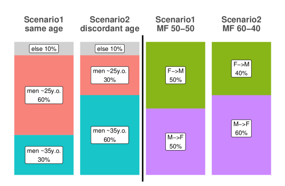
Web Figure 6: Graphic illustration of the simulation setup. We consider two different scenarios for each epidemiological question of interest. (1) Age of male sources for young women between 15 and 24 (left panel); scenario “same age” has most young women infections attributable to young men around 25 who are of similar age to those infected, whereas in scenario “discordant age” most such transmissions are attributable to older men around 35. (2) Proportions of male-to-female and female-to-male events; for scenario “MF 50-50” the two transmission directions have equal incidents, while in scenario “MF 60-40” there are slightly more MF transmissions which contribute to 60% of total infections.

1: age structure of male sources for infections in young women

We consider two scenarios with different setup in the BVN mixture model of the spatial density function $f_{1}(\cdot)$ for MF transmissions:

• same age: For women aged between 15-24, infections from younger men take the majority; here, for density function $f_{1}(\cdot)$, we set the component centered at $(35,20)^{T}$ (i.e., older men sourced transmission) to have mixture weight $0.3$, and the component centered at $(25,20)^{T}$ (i.e., younger men sourced transmission) to have mixture weight $0.6$.

• discordant age: For women aged between 15-24, infections from older men take the majority; here, for function $f_{1}(\cdot)$, we set the component centered at $(35,20)^{T}$ to have mixture weight $0.6$, and the component centered at $(25,20)^{T}$ to have mixture weight $0.3$.

For each scenario, the other $10\%$ probability mass for MF transmissions is spread across all other bivariate normal components of the density function $f_{1}$.

2. proportions of MF and FM transmission events

We consider the following two scenarios with different value choices for the type probability $\mathbf{p}$:

• MF 50-50: There are equal proportions of MF and FM events, and each contribute to about 50% of all real transmission events; we set 25% of events to be non-transmission events, and thus we have $p_{0}=0.25,p_{-1}=p_{1}=0.375$.

• MF 60-40: There are more MF events than FM events, and MF events contribute to about 60% of all transmissions; again, we set 25% of events to be non-transmissions, and thus we have $p_{0}=0.25,p_{-1}=0.3,p_{1}=0.45$.

To simulate the spatial patterns, we use $6$ different BVN mixture components to construct the three density functions $f_{0},f_{-1},f_{1}$; for the signal distributions, we set $\mu_{\ell}=2$, $\mu_{d}=1.5,\mu_{-d}=-1.5$, and $\sigma_{\ell}^{2}=\sigma_{d}^{2}=1$.

For each simulation, we run the Bayesian MCMC sampler for $3000$ iterations with a $1000$-iteration burn-in period, and adopt the following hyper-parameters for the priors: $a_{0}=1,b_{0}=0.02$ (prior for $\gamma$), $\nu_{0}=2,\sigma_{0}^{2}=1$ (priors for $\sigma_{\ell}^{2}$ and $\sigma_{d}^{2}$), $q_{i}=1,i=1,2,3$ (prior for $\mathbf{p}$), $\theta_{0}=(0,0)^{T},\Sigma_{0}=\bigl{(}\begin{smallmatrix}10^{4}&0\\ 0&10^{4}\end{smallmatrix}\bigr{)}$ (priors for $\theta_{kh}$’s), $\nu=2,S_{0}=I_{2}$ (priors for $\Sigma_{kh}$’s), and $a=2,b=3$ (priors for $\alpha_{k}$’s). We have experimented with various hyper-parameter values and have found that the results are not sensitive to value changes within reasonable ranges.

Simulation study results

In addition to the posterior medians results shown in the main text, within each simulation run, we can also look at the posterior credible intervals. In Web Figure 7, we plot the 95% posterior credible intervals for the proportions of male source age groups in each scenario in the top row, and for proportions of each transmission directions as well in the bottom row. For each sample size $N$ and scenario setting, the plotted credible intervals are acquired from five (5) randomly selected simulations among $100$ total runs. We can see that the majority of these credible intervals do cover the truth (marked by dashed lines in each sub-plot), and when $N$ gets larger, the credible intervals get narrower, indicating less uncertainty when more data are available.

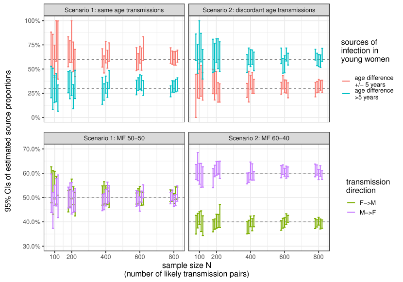
Web Figure 7: 95% posterior credible intervals of the simulation study. Results are shown for five (5) randomly selected simulation run for each $N$ and each scenario. Each error bar shows the 95% posterior credible interval. The true parameter values are marked in dashed lines in each subplot.

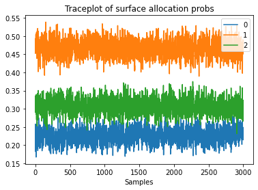
(a) Traceplot of the surface probabilities (entries of $\mathbf{p}$). $0=$ non-event, $1=$ MF transmission surface, $2=$ FM transmission surface.

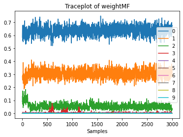
(b) Traceplot of the BVN component mixture weights (with label switching accounted for) for the male-to-female (MF) transmission surface. Each number/color represents a unique BVN component.

Web Figure 8: Traceplots for transmission surface type probabilities (subplot (a)) and BVN mixture component weights for FM surface (subplot (b)) throughout the 3000 iterations of the MCMC sampler. Example from a randomly picked simulation run with $N=600$.

Moreover, within each run of the simulation study, we can also inspect the MCMC traceplots (such as the ones shown in Web Figure 8) to check for convergence and inference quality, which is also similarly done for the real data case study. For example, in subplot (a), we plot the values of entries in $\mathbf{p}$ (the probability/probability vector for the three transmission types) sampled across all 3000 iterations of the MCMC sampler, where the three lines represent MF, FM and non-event transmission surfaces from top to bottom. Inspecting this traceplot, we can see that the sampled probability values stabilize after the initial 500 iterations or so (used as the “burn-in” period) and, in later iterations, fluctuate around a value close to ground truth (in this case, MF and FM probabilities have an approximate ratio of 60% versus 40%), which is an indicator of convergence. Also, in subplot (b), we show the traceplot of the sampled mixture weights (of the BVN components) for the MF surface. Again, we see that the weights have stabilized in later iterations after some exploration in the early steps, and there are three dominating components where the two biggest ones have weights around 0.6 and 0.3, respectively, which is very close to the true mixture weight values. Note that in real data analysis, we can also use the traceplots as a graphical diagnostic tool to check MCMC convergence.

Web Appendix C: Supplemental Materials for the Case Study

Full analysis with flexible point types

In the full analysis, we pre-specify$\mu_{d}=1.5$ and $\mu_{-d}=-1.5$ to imply that the $d_{i}$’s with $i=1$ are centered around $0.817$ and the $d_{i}$’s with $i=-1$ are centered around $0.182$. We note that analysis results are not considerably sensitive to the choices of these parameters, and through experiments, we’ve found that altering these values within a reasonable range produces consistent results.

Moreover, for a pair with $d_{i}=1$ or $0$ (extremely large or small direction scores), in the inference process, we conditionally assign it to the MF or FM surface depending on its $\ell_{i}$ score - if $c_{i}$ is sampled to be nonzero in the inference algorithm, then we would set $c_{i}=1$ if $d_{i}=1$ and otherwise set $c_{i}=-1$.

Additional analysis results

Here we provide a graphical illustration as supplement to Table 1 in the main text. As described in Section 5, our model (“model”) recognized more data points as real transmission events compared to the fixed-type analysis (“fixed”), thus effectively leveraging more information from the data.

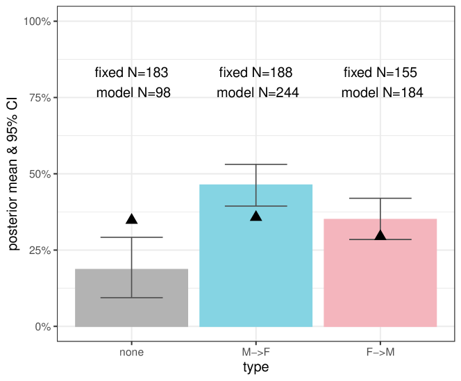
Web Figure 9: Proportions of data points assigned to different type labels (MF, FM or none) identified by the full model (colored bars), compared to partial analysis with fixed point types (marked by ’s). The colored bars show the posterior median proportions of type labels, with black errorbars showing the 95% credible intervals; the number of points assigned to each type (using posterior median numbers for the full model) is also annotated on the plot. The full model consistently identifies significantly more data points as MF or FM transmission events than the fixed model, while the relative ratios between MF and FM event counts are similar between the full and partial analyses (fixed: $\text{MF}/\text{FM}\approx 1.22$, full model: $\text{MF}/\text{FM}\approx 1.32$).

Source age distribution by specific recipient age groups

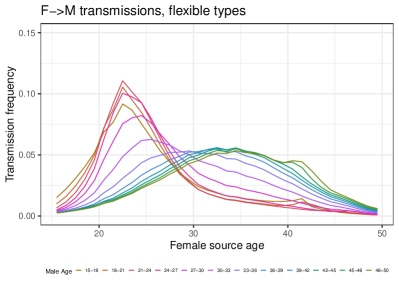
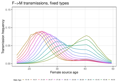
Web Figure 10: Source age distribution for recipients in each 3-year age band. Top row: results learned from full analysis without pre-fixing point type labels. Bottom row: results learned from the partial analysis with pre-fixed point types. Left column: male sources and female recipients; right column: female sources and male recipients.

In Web Figure 10, for each 3-year age band of recipients, we plot the relative frequency curve for the age of heterosexual sources. On the left column, we show inferred results for male to female (MF) transmissions – each curve corresponds to each 3-year age group of female recipients (e.g., the leftmost curve represents the age distribution of male sources for women between 15 to 18); on the right column, we show results in the same manner for female to male (FM) transmissions. The full analysis (flexible point types) results are presented in the top row, while partial analysis (fixed point types) results are shown on the bottom.

We can see that for different age groups of recipients, the age distributions of their sources could be very different. On the left column (male-to-female transmissions), we can see that younger women may get infected by both younger and older men, but older women main get infected by similarly aged men. On the right side (female-to-male transmissions), we see a more age assortative behavior (young men mainly get infected by young women and older men get infected by older women); however, we also see a bump of female sources at around age 40 for younger men, which also agrees with the general findings discussed in the main paper.

How our model leverages uncertain data points

A central feature of our proposed model is to probabilistically and flexibly classify point types, particularly for the ones with medium direction scores and/or low linkage scores (the uncertain points). Those uncertain points play an important role in inferring the spatial patterns, borrowing information across different types, and helping leverage spatial information for point type allocation.

For a data point $i$, the posterior mean probability vector $\hat{p}_{i}=(\hat{p}_{i,0},\hat{p}_{i,1},\hat{p}_{i,-1})^{T}$ for its type indicator $c_{i}$ represents the level of uncertainty we have about its type. (Here, for example, $\hat{p}_{i,1}$ is the relative frequency of $i$ being assigned to the MF surface across all posterior samples. ) If the entropy of $\hat{p}_{i}$ is high, then we have high uncertainty about $i$’s type.

In Web Figure 11, we plot the 77 data points with classification entropy $>0.8$ (as a reference, $(0.1,0.2,0.7)^{T}$ would have entropy $=0.802$). On the left, the points are colored according to the types they are most frequently assigned to in the posterior samples (as in the sampling iterations of the full model). On the right, the color represents the type a point would get assigned to given fixed pre-classification (as in the flexbile-type analysis).

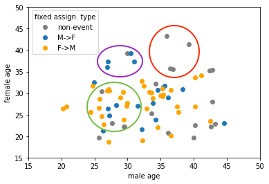
Web Figure 11: Flexible-type data points with classification entropy $>0.8$ (77 points in total). Left: point color represents the most frequent type assignment; right: point color represents the fixed threshold classification.

One of the most distinct differences between the two plots is the classification of the three points in the upper right corner (inside the red circle). In the full model, they tend to be assigned to the FM surface as their linkage scores are relatively high (close to the $0.6$ fixed threshold) and their locations are close to the FM surface mass near $(40,40)$. Therefore, these points contribute (at least probabilistically) to characterizing the transmission flow patterns from older women to older men.

Another notable difference is within the green circles of the two plots. The full model would, in fact, switch the type allocations for most of those points across the iterations of the inference algorithm, since they are mostly flexible-type points with close-to-threshold direction and linkage scores. (Note that this region is a high-density region for both MF and FM surfaces.) By exploring the possible configurations of data point classification, the model effectively allows spatial information to be shared between different surfaces (especially between MF and FM transmission surfaces) while accounting for the uncertainty in the point types. This is exactly what we hope to achieve through a hierarchical model.

Finally, within the purple circles, the two points at the upper left corner tend to be more frequently classified as FM transmission events, as opposed to the MF classification using fixed thresholds. This is actually in part due to the slightly different spatial patterns of the two transmission directions learned from all other data points: in the FM surface (bottom-middle panel in Figure 5 of the main text), there is a slightly denser mass for older-women to younger-men transmissions, and hence these two points tend to be assigned to the FM surface slightly more frequently. This is an example of how the learned spatial patterns help inform data point classification throughout the iterations of the inference procedure, thanks to joint modeling of the spatial process and the signal distributions as described in Section 2 of the main text.

References

- Adams et al. (2009) Adams, R. P., Murray, I., and MacKay, D. J. (2009). Tractable nonparametric Bayesian inference in Poisson processes with Gaussian process intensities. In Proceedings of the 26th Annual International Conference on Machine Learning, pages 9–16.
- Banerjee et al. (2003) Banerjee, S., Carlin, B. P., and Gelfand, A. E. (2003). Hierarchical modeling and analysis for spatial data. Chapman and Hall/CRC.
- Bauer et al. (2016) Bauer, C., Wakefield, J., Rue, H., et al. (2016). Bayesian penalized spline models for the analysis of spatio-temporal count data. Statistics in medicine 35, 1848–1865.
- Bbosa et al. (2020) Bbosa, N., Ssemwanga, D., Ssekagiri, A., et al. (2020). Phylogenetic and demographic characterization of directed HIV-1 transmission using deep sequences from high-risk and general population cohorts/groups in Uganda. Viruses 12, 331.
- Berke (2004) Berke, O. (2004). Exploratory disease mapping: kriging the spatial risk function from regional count data. International Journal of Health Geographics 3, 1–11.
- Best et al. (2005) Best, N., Richardson, S., and Thomson, A. (2005). A comparison of Bayesian spatial models for disease mapping. Statistical methods in medical research 14, 35–59.
- Brix and Diggle (2001) Brix, A. and Diggle, P. J. (2001). Spatiotemporal prediction for log-gaussian cox processes. Journal of the Royal Statistical Society: Series B (Statistical Methodology) 63, 823–841.
- Cressie (2015) Cressie, N. (2015). Statistics for spatial data. John Wiley & Sons.
- De Oliveira et al. (2017) De Oliveira, T., Kharsany, A. B., Gräf, T., et al. (2017). Transmission networks and risk of HIV infection in KwaZulu-Natal, South Africa: a community-wide phylogenetic study. The lancet HIV 4, e41–e50.
- Eisinger and Fauci (2018) Eisinger, R. W. and Fauci, A. S. (2018). Ending the HIV/AIDS pandemic. Emerging infectious diseases 24, 413.
- Escobar and West (1995) Escobar, M. D. and West, M. (1995). Bayesian density estimation and inference using mixtures. Journal of the american statistical association 90, 577–588.
- Fauci and Lane (2020) Fauci, A. S. and Lane, H. C. (2020). Four decades of HIV/AIDS—much accomplished, much to do. New England Journal of Medicine 383, 1–4.
- Givens et al. (1997) Givens, G. H., Smith, D., and Tweedie, R. (1997). Publication bias in meta-analysis: a Bayesian data-augmentation approach to account for issues exemplified in the passive smoking debate. Statistical Science 12, 221–250.
- Glynn et al. (2001) Glynn, J. R., Caraël, M., Auvert, B., et al. (2001). Why do young women have a much higher prevalence of HIV than young men? a study in Kisumu, Kenya and Ndola, Zambia. Aids 15, S51–S60.
- Grabowski et al. (2017) Grabowski, M. K., Serwadda, D. M., Gray, R. H., et al. (2017). HIV prevention efforts and incidence of HIV in Uganda. New England Journal of Medicine 377, 2154–2166.
- Gschlößl and Czado (2008) Gschlößl, S. and Czado, C. (2008). Modelling count data with overdispersion and spatial effects. Statistical papers 49, 531–552.
- Hall et al. (2021) Hall, M., Golubchik, T., Bonsall, D., et al. (2021). Demographic characteristics of sources of HIV-1 transmission in Zambia. medRxiv .
- Heikkinen and Arjas (1998) Heikkinen, J. and Arjas, E. (1998). Non-parametric Bayesian estimation of a spatial Poisson intensity. Scandinavian Journal of Statistics 25, 435–450.
- Heuveline (2004) Heuveline, P. (2004). Impact of the HIV epidemic on population and household structure: the dynamics and evidence to date. AIDS (London, England) 18, S45.
- Hu and Bradley (2018) Hu, G. and Bradley, J. (2018). A Bayesian spatial–temporal model with latent multivariate log-gamma random effects with application to earthquake magnitudes. Stat 7, e179.
- Huber (2011) Huber, M. (2011). Spatial point processes. Handbook of Markov Chain Monte Carlo pages 253–278.
- Hyman et al. (1994) Hyman, J. M., Li, J., and Stanley, E. A. (1994). Threshold conditions for the spread of the HIV infection in age-structured populations of homosexual men. Journal of theoretical biology 166, 9–31.
- Ishwaran and James (2004) Ishwaran, H. and James, L. F. (2004). Computational methods for multiplicative intensity models using weighted gamma processes: proportional hazards, marked point processes, and panel count data. Journal of the American Statistical Association 99, 175–190.
- Jewkes et al. (2010) Jewkes, R. K., Dunkle, K., Nduna, M., and Shai, N. (2010). Intimate partner violence, relationship power inequity, and incidence of HIV infection in young women in South Africa: a cohort study. The lancet 376, 41–48.
- Ji et al. (2009) Ji, C., Merl, D., Kepler, T. B., and West, M. (2009). Spatial mixture modelling for unobserved point processes: Examples in immunofluorescence histology. Bayesian analysis (Online) 4, 297.
- Johnson et al. (2019) Johnson, O., Diggle, P., and Giorgi, E. (2019). A spatially discrete approximation to log-Gaussian Cox processes for modelling aggregated disease count data. Statistics in medicine 38, 4871–4887.
- Karim et al. (2010) Karim, Q. A., Sibeko, S., and Baxter, C. (2010). Preventing HIV infection in women: a global health imperative. Clinical Infectious Diseases 50, S122–S129.
- Kim and Kottas (2022) Kim, H. and Kottas, A. (2022). Erlang mixture modeling for poisson process intensities. Statistics and Computing 32, 1–15.
- Kottas et al. (2008) Kottas, A., Duan, J. A., and Gelfand, A. E. (2008). Modeling disease incidence data with spatial and spatiotemporal Dirichlet process mixtures. Biometrical Journal: Journal of Mathematical Methods in Biosciences 50, 29–42.
- Kottas and Sansó (2007) Kottas, A. and Sansó, B. (2007). Bayesian mixture modeling for spatial Poisson process intensities, with applications to extreme value analysis. Journal of Statistical Planning and Inference 137, 3151–3163.
- Kutoyants (2012) Kutoyants, Y. A. (2012). Statistical inference for spatial Poisson processes, volume 134. Springer Science & Business Media.
- Le Vu et al. (2019) Le Vu, S., Ratmann, O., Delpech, V., et al. (2019). HIV-1 transmission patterns in men who have sex with men: insights from genetic source attribution analysis. AIDS research and human retroviruses 35, 805–813.
- Leitner and Romero-Severson (2018) Leitner, T. and Romero-Severson, E. (2018). Phylogenetic patterns recover known HIV epidemiological relationships and reveal common transmission of multiple variants. Nature microbiology 3, 983–988.
- Lo and Weng (1989) Lo, A. Y. and Weng, C.-S. (1989). On a class of Bayesian nonparametric estimates: II. Hazard rate estimates. Annals of the Institute of Statistical Mathematics 41, 227–245.
- Mohebbi et al. (2008) Mohebbi, M., Mahmoodi, M., Wolfe, R., et al. (2008). Geographical spread of gastrointestinal tract cancer incidence in the Caspian Sea region of Iran: spatial analysis of cancer registry data. BMC cancer 8, 1–12.
- Mohebbi et al. (2014) Mohebbi, M., Wolfe, R., and Forbes, A. (2014). Disease mapping and regression with count data in the presence of overdispersion and spatial autocorrelation: a Bayesian model averaging approach. International journal of environmental research and public health 11, 883–902.
- Møller et al. (1998) Møller, J., Syversveen, A. R., and Waagepetersen, R. P. (1998). Log Gaussian Cox processes. Scandinavian journal of statistics 25, 451–482.
- Oliver (2012) Oliver, M. (2012). The US president’s emergency plan for AIDS relief: Gendering the intersections of neo-conservatism and neo-liberalism. International Feminist Journal of Politics 14, 226–246.
- Pettifor et al. (2008) Pettifor, A. E., Levandowski, B. A., MacPhail, C., et al. (2008). Keep them in school: the importance of education as a protective factor against HIV infection among young South African women. International journal of epidemiology 37, 1266–1273.
- Rasmussen (1999) Rasmussen, C. (1999). The infinite Gaussian mixture model. Advances in neural information processing systems 12,.
- Ratmann et al. (2019) Ratmann, O., Grabowski, M. K., Hall, M., et al. (2019). Inferring HIV-1 transmission networks and sources of epidemic spread in Africa with deep-sequence phylogenetic analysis. Nature communications 10, 1–13.
- Ratmann et al. (2020) Ratmann, O., Kagaayi, J., Hall, M., et al. (2020). Quantifying HIV transmission flow between high-prevalence hotspots and surrounding communities: a population-based study in Rakai, Uganda. The Lancet HIV 7, e173–e183.
- Risher et al. (2021) Risher, K., Cori, A., Reniers, G., et al. (2021). Age patterns of HIV incidence in eastern and southern Africa: a collaborative analysis of observational general population cohort studies. LANCET HIV 8,.
- Rodger et al. (2019) Rodger, A. J., Cambiano, V., Bruun, T., et al. (2019). Risk of HIV transmission through condomless sex in serodifferent gay couples with the HIV-positive partner taking suppressive antiretroviral therapy (PARTNER): final results of a multicentre, prospective, observational study. The Lancet 393, 2428–2438.
- Romero-Severson et al. (2016) Romero-Severson, E. O., Bulla, I., and Leitner, T. (2016). Phylogenetically resolving epidemiologic linkage. Proceedings of the National Academy of Sciences 113, 2690–2695.
- Rue and Held (2005) Rue, H. and Held, L. (2005). Gaussian Markov random fields: theory and applications. Chapman and Hall/CRC.
- Rue et al. (2009) Rue, H., Martino, S., and Chopin, N. (2009). Approximate Bayesian inference for latent Gaussian models by using integrated nested Laplace approximations. Journal of the royal statistical society: Series b (statistical methodology) 71, 319–392.
- Saul et al. (2018) Saul, J., Bachman, G., Allen, S., et al. (2018). Determined resilient empowered AIDS-free mentored and safe (DREAMS): What is the core package and why now. PLOS One 3,.
- Scire et al. (2020) Scire, J., Barido-Sottani, J., Kühnert, D., et al. (2020). Improved multi-type birth-death phylodynamic inference in BEAST 2. bioRxiv .
- Sharrow et al. (2014) Sharrow, D. J., Clark, S. J., and Raftery, A. E. (2014). Modeling age-specific mortality for countries with generalized HIV epidemics. PloS one 9, e96447.
- Taddy et al. (2012) Taddy, M. A., Kottas, A., et al. (2012). Mixture modeling for marked Poisson processes. Bayesian Analysis 7, 335–362.
- UNAIDS (2018) UNAIDS (2018). Miles to go: closing gaps, breaking barriers, righting justice, document jc2924. https://www.unaids.org/sites/default/files/media_asset/miles-to-go_en.pdf.
- van de Kassteele et al. (2017) van de Kassteele, J., van Eijkeren, J., and Wallinga, J. (2017). Efficient estimation of age-specific social contact rates between men and women. The Annals of Applied Statistics 11, 320–339.
- Vedel Jesen and Thorarinsdottir (2007) Vedel Jesen, E. B. and Thorarinsdottir, T. L. (2007). A spatio-temporal model for functional magnetic resonance imaging data–with a view to resting state networks. Scandinavian journal of statistics 34, 587–614.
- Wakefield (2007) Wakefield, J. (2007). Disease mapping and spatial regression with count data. Biostatistics 8, 158–183.
- Wilson and Halperin (2008) Wilson, D. and Halperin, D. T. (2008). “Know your epidemic, know your response”: a useful approach, if we get it right. The Lancet 372, 423–426.
- Wolpert and Ickstadt (1998) Wolpert, R. L. and Ickstadt, K. (1998). Poisson/gamma random field models for spatial statistics. Biometrika 85, 251–267.
- Wymant et al. (2018) Wymant, C., Hall, M., Ratmann, O., et al. (2018). PHYLOSCANNER: inferring transmission from within-and between-host pathogen genetic diversity. Molecular biology and evolution 35, 719–733.
- Xi et al. (2022) Xi, X., Spencer, S. E., Hall, M., et al. (2022). Inferring the sources of HIV infection in Africa from deep sequence data with semi-parametric Bayesian Poisson flow models. Journal of the Royal Statistical Society Series C (Applied Statistics) .
- Zhang et al. (2020) Zhang, Y., Wymant, C., Laeyendecker, O., et al. (2020). Evaluation of Phylogenetic Methods for Inferring the Direction of Human Immunodeficiency Virus Transmission: HIV Prevention Trials Network (HPTN) 052. Clinical Infectious Diseases 72, 30–37.
- Zhao and Kottas (2021) Zhao, C. and Kottas, A. (2021). Modelling for Poisson process intensities over irregular spatial domains. arXiv preprint arXiv:2106.04654 .
- Zhou et al. (2015) Zhou, Z., Matteson, D. S., Woodard, D. B., et al. (2015). A spatio-temporal point process model for ambulance demand. Journal of the American Statistical Association 110, 6–15.