Self-supervised network distillation: an effective approach to exploration in sparse reward environments

Abstract

Reinforcement learning can solve decision-making problems and train an agent to behave in an environment according to a predesigned reward function. However, such an approach becomes very problematic if the reward is too sparse and so the agent does not come across the reward during the environmental exploration. The solution to such a problem may be to equip the agent with an intrinsic motivation that will provide informed exploration during which the agent is likely to also encounter external reward. Novelty detection is one of the promising branches of intrinsic motivation research. We present Self-supervised Network Distillation (SND), a class of intrinsic motivation algorithms based on the distillation error as a novelty indicator, where the predictor model and the target model are both trained. We adapted three existing self-supervised methods for this purpose and experimentally tested them on a set of ten environments that are considered difficult to explore. The results show that our approach achieves faster growth and higher external reward for the same training time compared to the baseline models, which implies improved exploration in a very sparse reward environment. In addition, the analytical methods we applied provide valuable explanatory insights into our proposed models.

1 Introduction

The development of reinforcement learning (RL) methods has achieved much success over the last decade, since together with advances in computer vision [28, 21], it became possible to teach agents to solve various tasks, play computer games [33] (see overview in [49]) even surpassing human players [34]. Nevertheless, these single tasks require very long training times and a lot of computational resources. Coping with complex environments such as the real world is still a challenge. There are several research opportunities, one of them being the search for more efficient learning methods.

The complex environments with sparse rewards pose a special challenge for RL approaches. The most popular computational approach to make RL more efficient is based on a concept of intrinsic motivation (IM) [8]. IM has a strong biological basis [41, 35], since it is observed among higher animals, especially in humans, engaging them in various activities. Intrinsic motivations appear early after birth and guide the biological agents during their entire lives. IM is considered one of the prerequisites for open-ended (or, life-long) learning. If we want to achieve this capacity with artificial agents [38], we have to master this first step and equip them with an ability to generate their own goals and acquire new skills [22]. Therefore, computational approaches concerned with IMs and open-ended development provide the potential in this direction leading to more intelligent systems, in particular those capable of improving their own skills and knowledge autonomously and indefinitely [8, 7].

The concept of intrinsic (and extrinsic) motivation was first studied in psychology [41] and later it entered the RL literature [11, 47, 10]. The first taxonomy of computational models appeared in [37] where the concept of motivation is divided into external and internal, depending on a mechanism that generates motivation for the agent. External motivation assumes the source of motivation coming from outside the agent, and it is always associated with a particular goal in the environment. If the motivation is generated within the structures that make up the agent, this implies an internal motivation.

Another dimension for the differentiation, extrinsic or intrinsic, is less obvious (see also [35]). Extrinsic motivations pertain to behaviors whenever an activity is performed in order to attain some separable outcome. Some variability exists in this context since these behaviors can vary in the extent to which they represent self-determination (see the details in [41]). On the other hand, intrinsic motivation is defined as doing an activity for its inherent satisfaction. IM has been operationally defined in various ways, backed up by different psychological theories which point to some uncertainty in what it exactly means. Nevertheless, a solution of an operational definition of IMs has been proposed [7] in terms of processes that can drive the acquisition of knowledge and skills in the absence of extrinsic motivations. Furthermore, the author proposes (and explains why) a new term of epistemic motivations as a suitable substitution for intrinsic motivations. Despite some uncertainty, intrinsic motivation has remained a well-coined term in the literature.

Intrinsic motivation is a crucial factor that helps the agent not only to remain in open-ended learning, hence solving a variety of tasks [38], but it also helps to solve a single task with extremely sparse rewards. In this paper, we focus on this case.

There exists a variety of approaches aiming to use IM-based signal for agent learning. Information-theoretic view on IM is well represented in the literature, involving the concepts of novelty, surprise, and skill learning. The recent review [5] suggests that novelty and surprise can assist the building of a hierarchy of transferable skills that abstracts dynamics and makes the exploration process more robust. In this context, abstraction is a key feature of the agent architecture where it makes sense to introduce learning mechanisms to enforce the formation of proper internal representations that lead to improved agent performance.

Learning appropriate internal representations from unlabelled input data (e.g. images) for the purpose of solving various problems is in general a useful task in machine learning. This can be achieved in various ways (related methods are mentioned in Sec. 2), including supervised end-to-end (deep) learning, self-supervised autoencoders, unsupervised feature extractors (such as contrastive divergence learning) and RL-based approaches where a certain loss function is optimized.

As our main contribution, we identified shortcomings of the Random Network Distillation model (RND) [14] that served as a starting point for our work. RND is a novelty detection method that uses two models, the target model and the predictor model, both being fed by the current state as their input. The predictor model attempts to imitate the target model, and their difference (in terms of generated features) is used for intrinsic motivation. However, the RND method requires good initialization of the target model, has a low variance of intrinsic rewards, and loses the motivational signal, which is caused by the adaptation of the predictor model.

To address these shortcomings, in this contribution, we introduce a class of motivational methods based on the exploitation of the distillation error as novelty detection. To provide features with higher variance and better sensitivity for novelty detection, we use self-organized regularization of the target model. Our methods were able to use more feature space dimensions compared to RND (which has an impact on the size of the distillation error) and more importantly, the distances between representations of very similar states increased, which achieved a better ability to distinguish them from each other and thus the task for the predictor model became more complex. This led to an increase in the variance of the intrinsic reward and a slowdown in the adaptation of the predictor model. In particular, we adapted three existing self-supervised methods. The developed methodologies were tested on a set of environments that are considered difficult to explore. The overall concept is shown in Figure 1.

Using these methods, we were able to solve hard exploration seeds for ProcGen and the complete first level of the infamous Atari game – Montezuma’s Revenge, which, as far as we know, has never been finished using internal motivation methods. Overall, our models achieved excellent performance in most environments, and we provide insights based on our analyses, why this could be the case.

Our research goal was not to solve a general problem of RL, but as in many similar papers (see the related work) we focused on a set of challenging environments of a certain type (complex Atari games) with naturally sparse rewards. We also add challenging ProcGen games, since their authors provided hard exploration seeds, making the PPO algorithm unable to solve the tasks, even with a larger IMPALA model [17].

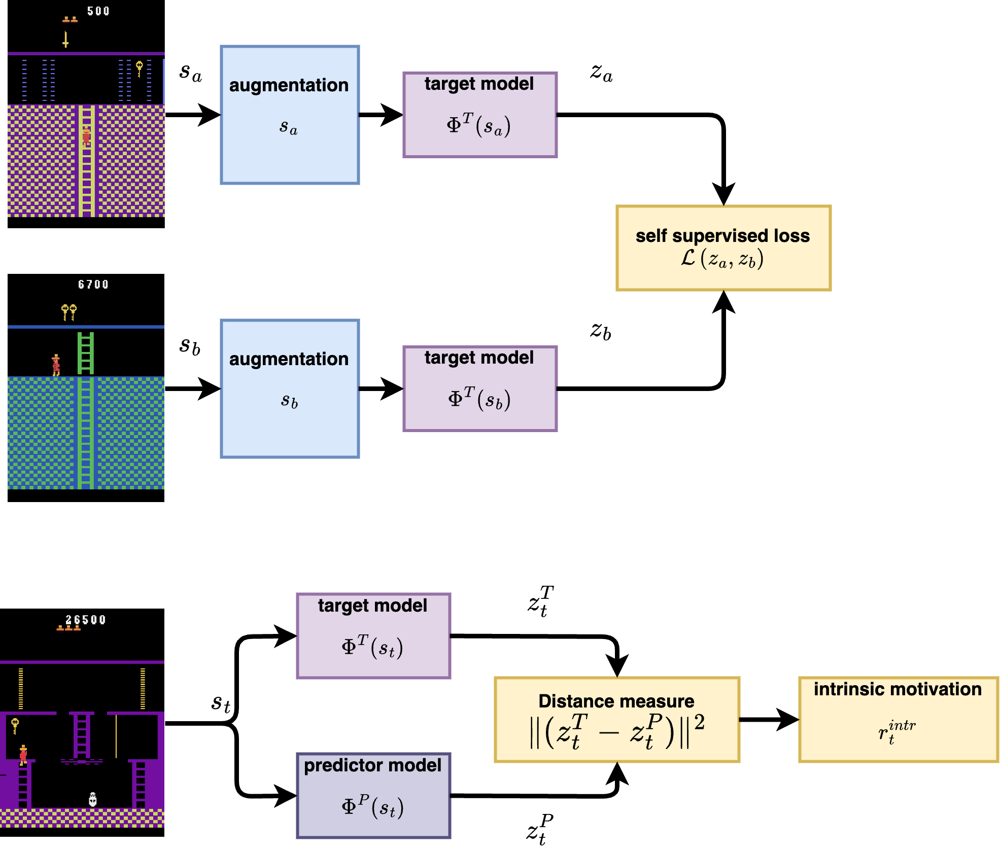
Figure 1: Self-supervised network distillation (SND) principle. The proposed method consists of two main parts. Top: Self-supervised learning of the suitable features for the target model. Bottom: Calculation of the intrinsic reward by target model distillation, using the squared Euclidean distance between the models’ outputs.

The rest of the paper is organized as follows. Section 2 relates our work in a wider and narrower context. Section 3 describes the methods that we introduced and tested in this work. Section 4 explains in detail all experiments performed. Section 5 provides the discussion about the achieved results, the limitations of our models and hints for further extensions. Section 6 concludes the paper by summarizing the main take-home messages.

2 Related work

We first provide the wider conceptual context to our work, and then focus more on methods that are closely related to our models. According to the prevailing view, the approaches to IM can be divided into two main categories with adaptive motivations. Knowledge-based approach is focused on the acquisition of the world knowledge of and it draws on the theory of drives, theory of cognitive dissonance and optimal incongruity theory. Competence-based approach focuses on the acquisition of skills by motivating the agent to achieve a higher level of performance in the environment, which means to acquire desired actions to achieve self-generated goals. Its psychological basis includes the theory of effectance and the theory of flow.

The knowledge-based category focusing on exploration can be divided into prediction-based, novelty-based and information-based approaches [4]. Prediction-based approaches use the prediction error as an intrinsic reward signal. The source of error can be a forward model (e.g. [51, 12, 39]), a generative model [55] (e.g. based on a variational auto-encoder [27]) or disagreement in a learned world model [43]. Exploration with Mutual Information (EMI) [25] extracts predictive signals that can be used to guide exploration based on forward prediction in the representation space. Model-based Active eXploration (MAX) [46] uses an ensemble of forward models to plan to observe novel events.

Information approaches use quantities from information theory [45], such as information gain, mutual information, entropy and try to maximize the information obtained by the agent from the environment. Variational Information Maximizing Exploration (VIME) [23] approximates the environment dynamics and uses the information gain of the learned dynamics model as an intrinsic reward. Random Encoders for Efficient Exploration (RE3) [44] is an exploration method that utilizes state entropy as an intrinsic reward. For more details, we recommend surveys [13, 4, 56].

In a narrower context, our work falls into the area of novelty-based approaches that monitor the state novelty. The first models exploited the count-based approach [52]. This approach is impractical for large or continuous state spaces and it was extended by introducing pseudo-count and neural density models [36, 32, 31]. A similar method to pseudo-count was used by a random network distillation (RND) model [14] with a lower complexity. The never-give-up framework [6] learns intrinsic rewards composed of episodic and life-long state novelty (which is detected by an RND model). BYOL-Explore [19] is one of the recent methods using self-supervised learning in the context of exploration and intrinsic rewards.

Self-supervised learning is a paradigm of machine learning when the agent does not have any externally labeled data. The goal is to use the information in the data itself and prepare the model to perform another task. Self-supervised learning also started to be used in the field of state representation learning [30], it has proven to be a suitable method for creating the feature space [2] and has also found its use in reinforcement learning [50, 19]. Contrastive learning [15] is a method of self-supervised learning minimizing a discriminative loss function that drives the similarity metric to be small for pairs from the same category, and large for pairs from different categories. Several different objective functions have been proposed, e.g. Noise Contrastive Estimation (NCE) [20], InfoNCE [53], or multi-class $N$-pair loss [48]. Another approach to self-supervised learning is based on regularization (non-contrastive methods). In this case, the model sees only positive examples (data points from the same category) and generates a feature space based on various regularization losses like invariance and covariance loss in the case of Barlow Twins model [57], triple variance-invariance-covariance losses in VICReg model [9], or other priors like proportionality, variability, slowness principle, or repeatability [24]. Bootstrap Your Own Latent (BYOL) [18] relies on two neural networks, referred to as online and target networks that interact and learn from each other.

3 Methods

The decision-making problem in the environment using RL is formalized as a Markov decision process defined as a 5-tuple ($\mathcal{S,A,T,R},\gamma$) consisting of a state space $\mathcal{S}$ with actions $s_{t}$, action space $\mathcal{A}$ with actions $a_{t}$, transition function $\mathcal{T}_{a}(s,s^{\prime})=P(s_{t+1}=s^{\prime}|s_{t}=s,a_{t}=a)$, reward function $\mathcal{R}_{a}(s,s^{\prime})$ specifying the immediate (external) reward after transition from $s$ to $s^{\prime}$ with action $a$, and a discount factor $\gamma$. The main goal of the agent is to maximize the discounted return $R_{t}=\sum_{k=0}^{\infty}\gamma^{k}r_{t+k}$ in each state, where $r_{t}$ is an immediate external reward at time $t$. The stochastic policy is defined as a state dependent probability function $\pi:\mathcal{S}\times\mathcal{A}\rightarrow[0,1]$ such that $\pi(s,a)=P(a_{t}=a|s_{t}=s)$ and $\sum_{a\in\mathcal{A}}\pi_{t}(s,a)=1$, and the deterministic policy is a mapping $\pi:\mathcal{S}\rightarrow\mathcal{A}$.

The methods searching for the optimal policy $\pi^{*}$, that maximizes the expected return $R$, can be divided into on-policy (the family of actor–critic algorithms) [42] and off-policy methods (the family of Q-learning algorithms) [33]. The actor–critic algorithms are based on two separate modules: an actor generates actions following the agent’s policy $\pi$ and a critic estimates the state value function $V^{\pi}$ defined for a stochastic policy as

$$V^{\pi}(s)=\sum_{a}\pi(s,a)\sum_{s^{\prime}}\mathcal{T}_{s,a,s^{\prime}}\left[\mathcal{R}_{s,a,s^{\prime}}+\gamma V^{\pi}(s^{\prime})\right]$$

or the state-action value function $Q^{\pi}$ defined as

$$Q^{\pi}(s,a)=\sum_{s^{\prime}}\mathcal{T}_{s,a,s^{\prime}}\left[\mathcal{R}_{s,a,s^{\prime}}+\gamma V^{\pi}(s^{\prime})\right].$$

The actor then updates its policy to maximize return $R$ based on the critic’s value function estimations.

In high-dimensional tasks, when one cannot use the Bellman equation, the common approach is to use function approximators (e.g., deep neural networks) for estimating the critic and the actor.

3.1 Intrinsic motivation and exploration

During the learning process, the agent must explore the environment to encounter an external reward and learn to maximize it. In the case of a deterministic policy, noise needs to be added to the state-conditional action selection. In both stochastic and deterministic cases, these are uninformed environmental exploration strategies. The problem arises if the external reward is very sparse and the agent cannot use these strategies to find the sources of the reward. In such a case, it is advantageous to use informed strategies which include the concept of intrinsic motivation.

In the context of RL, intrinsic motivation can be realized in various ways, but most often it is a new reward signal $r^{\rm intr}_{t}$ scaled by the parameter $\eta$ which is generated by what we refer to as the motivational module and is added to the external reward $r^{\rm ext}_{t}$

$$r_{t}=r_{t}^{\rm ext}+\eta\,r_{t}^{\rm intr}.$$ (1)

The goal of introducing such a new reward signal is to provide the agent with a source of information that is absent from the environment when the reward is sparse, and thus facilitate the exploration of the environment and the search for an external reward.

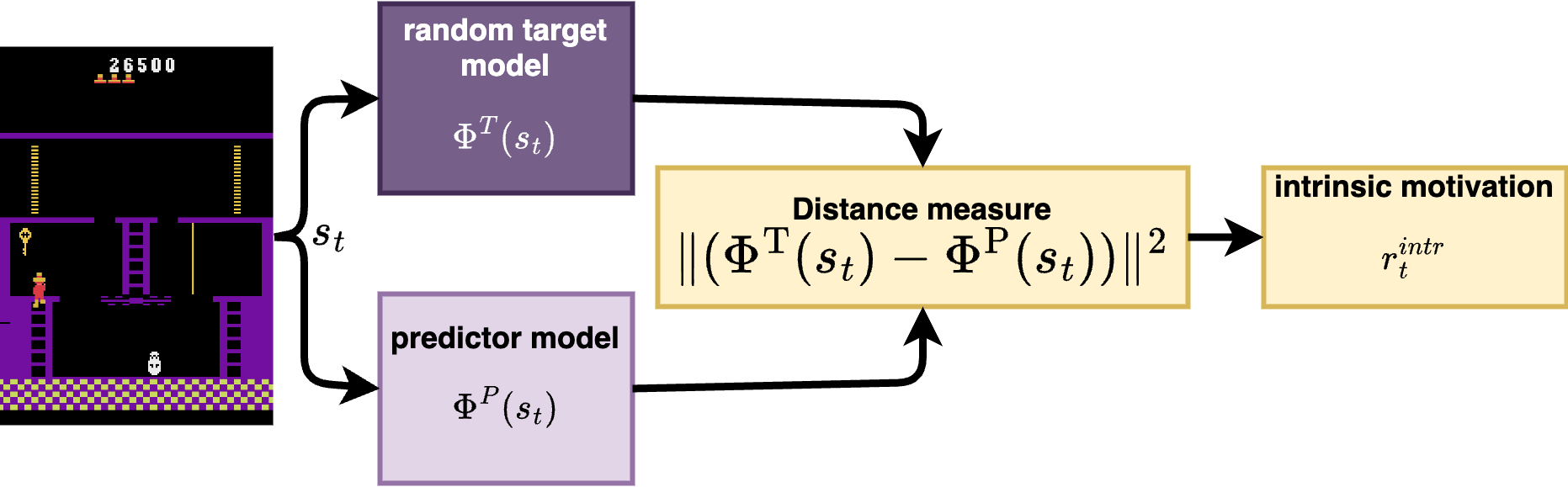
Figure 2: The basic principle of generating an exploration signal in Random Network Distillation.

3.2 Random Network Distillation

The Random Network Distillation (RND) [14] model shown in Figure 2 is a representative of methods based on novelty detection, belonging to the knowledge-based category of IM. The motivation module has two components: the target model $\Phi^{\rm T}$ that generates state representations and the predictor model $\Phi^{\rm P}$ that learns to estimate them. This process is called knowledge distillation. Intrinsic motivation, expressed as an intrinsic reward, is computed as the distillation error

$$r_{t}^{\rm intr}=\|(\Phi^{\rm T}(s_{t})-\Phi^{\rm P}(s_{t}))\|_{2}^{2}.$$ (2)

where $\|.\|^{2}_{2}$ denotes the squared $L_{2}$ vector norm. It is assumed that the predictor network $\Phi^{\rm P}$ will be able to more easily estimate the feature vectors for states it has seen multiple times, while new or rarely visited states will induce a large distillation error. The approach is simple and successful in environments with sparse reward but has two serious drawbacks: (1) It is necessary to properly initialize the random network and (2) over time, the signal of intrinsic motivation disappears due to sufficient adaptation of the learning network (a phenomenon that could be called generalization). In the section dedicated to analyzing the results of our method, we show that the RND method is able to detect only large changes in the state space, while small changes are almost invisible to it. This is a consequence of inappropriate features provided by the target model.

3.3 Self-supervised Network Distillation

We modified the concept of distillation of randomly initialized static network RND [14] and instead, we distilled a network that learns continuously using a self-supervised algorithm. We denote the methods SND.

Let $X=\{(s_{t},s_{t+1})_{n}\}_{n=1}^{N}$ be a minibatch of $N$ consecutive states from $\mathcal{S}$ that are sampled from collected trajectories and $\mathcal{Z}$ is a $D$-dimensional latent space of state representations. Let $S$ correspond to the set of actual states and $S_{\rm next}$ correspond to the set of next states (i.e. the set of left-column states and right-column states in each pair of states respectively). The shape of states $S$ and $S_{\rm next}$ in our experiments is a batch of stacked frames: $(N,C,H,W)$, where $N$ is the batch size, $C$ is the number of stacked frames, $H$ and $W$ are the height and the width of a frame. The architecture of the SND motivation module in general consists of a target model $\Phi^{\rm T}:\mathcal{S}\rightarrow\mathcal{Z}$ and a predictor model $\Phi^{\rm P}:\mathcal{S}\rightarrow\mathcal{Z}$ but with an essential difference that the network generating the target feature vectors (target model) also learns. The corresponding output $Z=\Phi^{\rm T}(S)$ is a $N$$\times$$D$ matrix (so the feature vectors are in rows). The predictor model optimizes the loss function

$$\mathcal{L}_{P}=\frac{1}{N}\sum_{s\in S}\|(\Phi^{\rm T}(s)-\Phi^{\rm P}(s))\|_{2}^{2}$$ (3)

The target model optimizes the loss function $\mathcal{L}_{T}$. Further, we introduce three methods (loss functions) for training the target model based on different self-supervised algorithms.

Both models are trained in the same loop as the actor and the critic. With a trained target model, the task for the predictor model becomes much more difficult, since the representations of the states move further apart and their distribution in the feature space becomes very different from the distribution of the states in the state space. This leads to the elimination of the shortcomings associated with the RND method. These properties of the SND methods are described in detail in section 7 devoted to the analysis of results. The schematic representation of the proposed approach is shown in Figure 3.

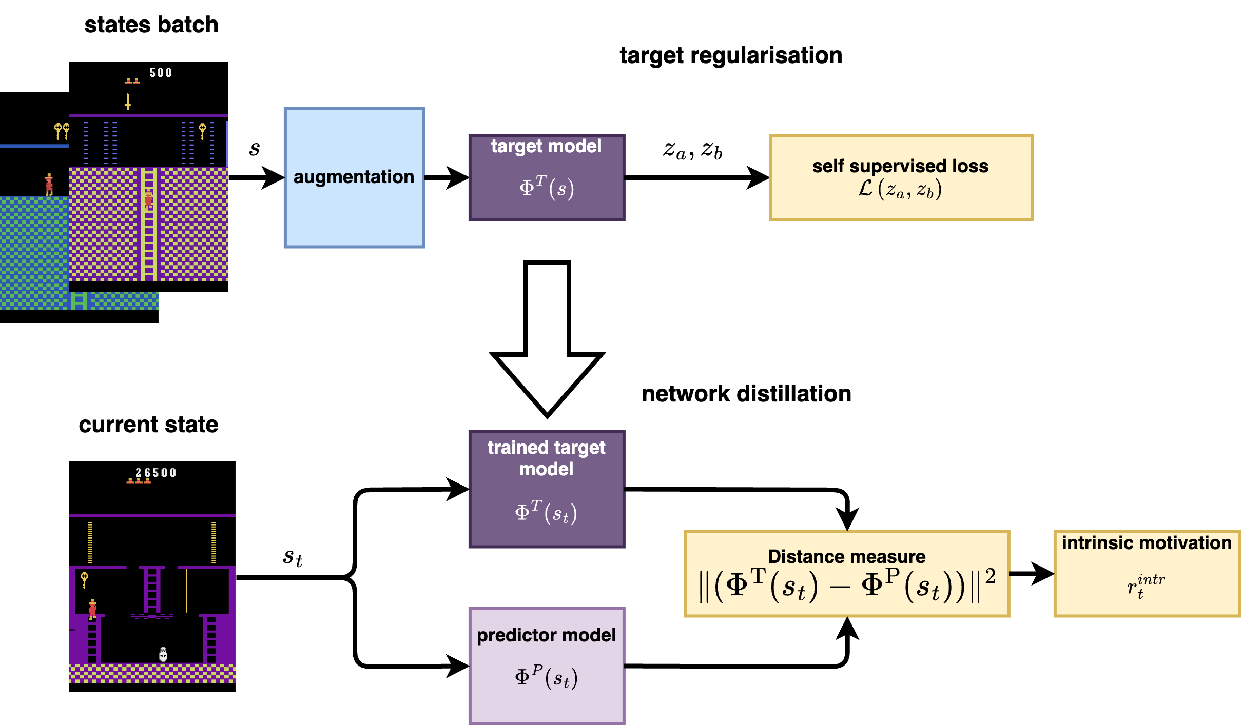
Figure 3: The basic principle of generating an exploration signal in Self-supervised Network Distillation. The calculation of the intrinsic reward is the same as for RND, but in these methods, the target model changes over time and generates a more complex feature space.

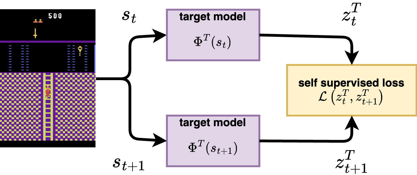
Figure 4: Training of the SND target model using two consecutive states and the self-supervised learning algorithm.

3.3.1 SND-V

This method uses a contrastive loss function [15]. Assume a batch of states $(S,S^{\prime})$ randomly sampled from the trajectory buffer. For each pair of states $(s_{n},s^{\prime}_{n})$ a target distance is generated. With probability $p=0.5$, $s_{n}=s^{\prime}_{n}$, in which case the target distance is set to $\tau_{n}=0$, otherwise $(s_{n}\neq s^{\prime}_{n})$ the target distance is set to $\tau_{n}=1$. The distance of predicted target model based features $\phi^{\rm T}(s_{n})$ and $\phi^{\rm T}(s^{\prime}_{n})$ is compared with the target distance in the mean squared error (MSE) loss.

For state preprocessing, we experimented with three augmentation schemes to learn suitable robust features:

1. uniform noise only, from the range $\langle-0.2,0.2\rangle$

2. random tile masking + uniform noise, tile sizes 2, 4, 8, 12, 16

3. random convolution filter + random tile masking + uniform noise.

Uniform noise was used for each pixel value, the remaining augmentations with $p=0.5$. The whole pipeline is shown in Figure 5. The idea of tiles masking can be supported by recently proposed self-supervised loss [3]. Random convolution was successfully used for a PPO agent in Procgen environment [29]. And finally, adding noise is a common augmentation process.

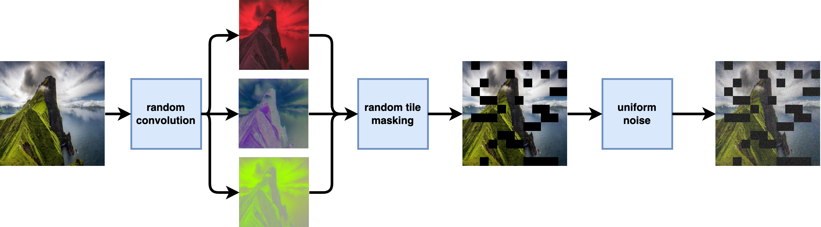
Figure 5: The scheme of the state augmentation pipeline.

The SND-V regularisation loss is defined as

$$\mathcal{L}_{T}=\sum_{n}(\tau_{n}-\|Z_{n}-Z^{\prime}_{n}\|^{2}_{2})^{2}$$ (4)

where $\|.\|^{2}_{2}$ is the squared Euclidean distance between $n$-th feature vectors $Z_{n}$ and $Z^{\prime}_{n}$. We also experimented with the loss function defined as

$$\mathcal{L}_{T}=\begin{cases}\|Z_{n}-Z^{\prime}_{n}\|^{2}_{2}&\text{if $\tau_{n}=0$}\\ \max(1-\|Z_{n}-Z^{\prime}_{n}\|^{2}_{2};0)&\text{otherwise}\end{cases}$$ (5)

This loss function pulls the feature vectors of similar states (when $\tau_{n}=0$) to one another by penalizing their squared distance. And on the contrary, it pushes away the feature vectors from one another, up to a certain limit when their distance exceeds one. However, we did not find any benefits of this loss.

3.3.2 SND-STD

This method uses the Spatio-Temporal DeepInfoMax (ST-DIM) algorithm [2]. The basic idea of the ST-DIM algorithm (see Figure 4) is to move closer the representations of two consecutive states on the output layer and the individual representations on the intermediate convolution layer that carry information about the location (global-local objective) and also to move closer the representations on the intermediate convolution layer for consecutive states (local-local objective).

In our context, the positive samples correspond to pairs of consecutive observations $(s_{t},s_{t+1})$ and negative samples correspond to pairs of non-consecutive observations $(s_{t},s^{*}_{t})$, where $s^{*}_{t}$ is a randomly sampled observation from the same minibatch. Hence, there are many more negative samples than positive samples.

Mathematically, ST-DIM uses two loss functions: the global-local objective (GL) and the local-local objective (LL), defined as [48]:

$$\mathcal{L}_{\rm GL}=-\sum_{h=1}^{H}\sum_{w=1}^{W}\log\frac{\exp(g_{h,w}(s_{t},s_{t+1}))}{\sum_{s_{t}^{*}\in S_{\rm next}}\exp(g_{h,w}(s_{t},s_{t}^{*}))}$$ (6)

$$\mathcal{L}_{\rm LL}=-\sum_{h=1}^{H}\sum_{w=1}^{W}\log\frac{\exp(f_{h,w}(s_{t},s_{t+1}))}{\sum_{s_{t}^{*}\in S_{\rm next}}\exp(f_{h,w}(s_{t},s_{t}^{*}))}$$ (7)

where the score function $g_{h,w}(s_{t},s_{t+1})=\Phi^{\rm T}(s_{t})W_{g}\Phi^{\rm T}_{(l,h,w)}(s_{t+1})^{\top}$ is defined as the unnormalized cosine similarity between transformed global features $\Phi^{\rm T}(s_{t})$ and local features $\Phi^{\rm T}_{(l,h,w)}(s_{t+1})$ of the intermediate convolution layer $l$ in $\Phi^{\rm T}$. Global features are transformed by (trained) matrix $W_{g}$ to the space of local features. Analogically, $f_{h,w}(s_{t},s_{t+1})=\Phi^{\rm T}_{(l,h,w)}(s_{t})W_{l}\Phi^{\rm T}_{(l,h,w)}(s_{t+1})^{\top}$ is the unnormalized cosine similarity between transformed local features $\Phi^{\rm T}_{(l,h,w)}(s_{t})$, by (trained) matrix $W_{l}$, and $\Phi^{\rm T}_{(l,h,w)}(s_{t+1})$. The resulting loss function is then defined as

$$\mathcal{L}=\frac{1}{MN}(\mathcal{L}_{\rm GL}+\mathcal{L}_{\rm LL}).$$ (8)

Following this objective function, the target model becomes a good feature extractor adapting to new states discovered by the agent. However, after initial tests, we found that the feature space formed by such an objective function tends to grow exponentially from a certain point until it eventually explodes. We provide a more detailed analysis of this problem in Section 5. The solution to this problem was to find a suitable regularization that was added to the existing loss function. We decided to minimize $L_{2}$-norm of logits represented by functions $f$ and $g$:

$$\mathcal{L}_{2}=p_{\rm GL}+p_{\rm LL}=\sum_{h=1}^{H}\sum_{w=1}^{W}(\|f_{h,w}\|+\|g_{h,w}\|)$$ (9)

Finally, we added one more regularization term $\mathcal{L}_{\sigma}$

$$\mathcal{L}_{\sigma}=-\sigma(\Phi^{\rm T}(s_{t}))$$ (10)

that maximizes the standard deviation $\sigma$ of the feature vector components and thus ensures that all dimensions of the feature space are used. The analysis (section 7) provides a more detailed justification for the introduction of this term.

The final objective function, with the scaling parameters $\beta_{1}=\beta_{2}=0.0001$ (found experimentally), was defined as

$$\mathcal{L_{T}}=\frac{1}{HW}(\mathcal{L}_{\rm GL}+\mathcal{L}_{\rm LL}+\beta_{1}\mathcal{L}_{2})+\beta_{2}\mathcal{L}_{\sigma}$$ (11)

3.3.3 SND-VIC

This method is based on VICReg algorithm [9] belonging to the class of non-contrastive self-supervised methods. The regularization function consists of three terms: the invariant term, which brings the feature vectors closer to each other, the variance term, which ensures that the feature vectors within one batch have different values and the covariance term, which ensures the decorrelation of the feature vectors and prevents information collapse. The original method does not need any negative samples, it only takes the input, creates two augmented versions, and their feature vectors are updated using the mentioned terms of the regularization function.

Our version uses the state $s_{t}$ and its successor $s_{t+1}$ (the same as ST-DIM, the simple diagram can be found in Figure 4) instead of two augmentations of the same state. The variance regularization term $\mathcal{L}_{v(Z)}$ is defined as a hinge function on the standard deviation of the features along the batch dimension

$$\mathcal{L}_{v(Z)}=\frac{1}{D}\sum_{d=1}^{D}\max(0;\tau-\sigma(Z_{d}))$$ (12)

where $Z_{d}$ is the $d$-${\rm th}$ component of all feature vectors from the batch $Z$, $\sigma$ is the actual standard deviation, and $\tau=1$ is a constant target value for the standard deviation. This term encourages the standard deviation inside the current batch to be equal to $\tau$ along each dimension, preventing collapse with all states mapped on the same feature vector.

The covariance regularization term $\mathcal{L}_{c(Z)}$ is defined as the sum of the squared off-diagonal coefficients of the covariance matrix $C(Z)$

$$\mathcal{L}_{c(Z)}=\frac{1}{(N-1)D}\sum_{i\neq j}[C(Z)]^{2}_{i,j}.$$ (13)

This term forces feature vector components to be uncorrelated, hence enabling each feature vector component to learn unique information.

The invariance criterion $\mathcal{L}_{s(Z,Z^{\prime})}$ between two batches $Z$ and $Z^{\prime}$ is defined as the mean-squared Euclidean distance between each pair of feature vectors

$$\mathcal{L}_{s(Z,Z^{\prime})}=\frac{1}{N}\sum_{b=1}^{N}\|Z_{n}-Z^{\prime}_{n}\|^{2}_{2}.$$ (14)

The overall loss $\mathcal{L}$ then takes the form

$$\mathcal{L}_{T}=\lambda\mathcal{L}_{s(Z,Z^{\prime})}+\mu\left[\mathcal{L}_{v(Z)}+\mathcal{L}_{v(Z^{\prime})}\right]+\nu\left[\mathcal{L}_{c(Z)}+\mathcal{L}_{c(Z^{\prime})}\right]$$ (15)

where the scaling parameters are set to $\lambda=1$, $\mu=1$ and $\nu=1/25$ based on recommendations in [9].

4 Experiments

Altogether we tested our methods on 10 environments (Atari and Procgen) that are considered difficult for exploration. These include 6 Atari environments: Montezuma’s Revenge, Gravitar, Venture, Private eye, Pitfall and Solaris. The agent receives a reward of +1 for each increase in the score, regardless of its value. It does not receive any other reward or punishment. The state (input to the models) is represented by four consecutive frames of pixels on greyscale, so the dimensionality of the state representation is 4$\times$96$\times$96. The action space is discrete, consisting of 18 actions, of which only some make sense (depending on the environment), the other actions have no impact on the environment.

We also tested 4 Procgen environments: Coinrun, Caveflyer, Jumper and Climber. Procgen is a set of procedurally generated environments, designed primarily for testing the agent’s generalisation [16]. The paper shows several problems for generalisation in RL, requiring special training and a huge number of samples. From our perspective, interesting findings (provided in Appendix B.1 of [16]) are that for several seeds, the baseline agent was not able to reach a non-zero score. Those seeds lead to hard exploration environments with only a single reward at the end. Together with a fast run of these environments (thousands of FPS on a single CPU core), this makes Procgen a very good candidate for our experiments. The state is represented by two consecutive stacked frames of RGB images, so the dimensionality of the state representation is 6$\times$64$\times$64. The action space is discrete, consisting of 15 actions. Preliminary experiments performed in [40] provided initial insights and led to the extensions in this work.

Before running the main experiments, we sought suitable values of hyperparameters. For this search, we chose Montezuma’s Revenge environment which represents a good compromise between game complexity and reward sparsity. This environment has been well studied (e.g. in [4, 14, 12, 13]) and therefore provides a good comparison for tuning hyperparameter.

4.1 Training setup

We ran 9 simulations for each environment, taking 128M steps for Atari and 64M steps for Procgen games. Before the main training, we tried three hand-selected settings of hyperparameters for individual motivational models (mainly the scaling of the motivational signal, or regularization terms) and we always chose the one that yielded the best results. These short probes lasted 32M (Atari) or 16M (Procgen) steps and consisted of 2 or 3 simulations.

All agents were trained with the PPO algorithm [42] using Adam optimizer [26] for the parameters of all modules. The basic agent consists of an actor and a critic, which are two multi-layer perceptrons sharing a common convolutional neural network (CNN) that processes the video input. The critic has two outputs (heads), one for estimating the value function for the external reward and the other for the intrinsic reward. We used the orthogonal weight initialisation with a magnitude $\sqrt{2}$. Model architectures are presented in Figures 6 to 8. The motivational module consists of two CNNs (the target and the learning network) which receive input from a single frame. The learning network contains two more linear layers to have an increased capacity over the target model.

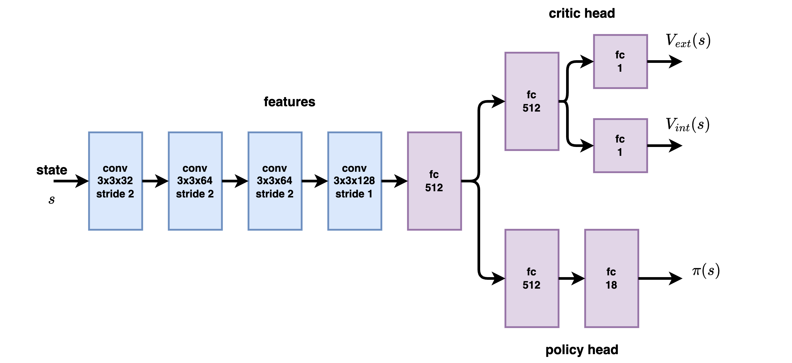
Figure 6: The PPO agent model architecture.

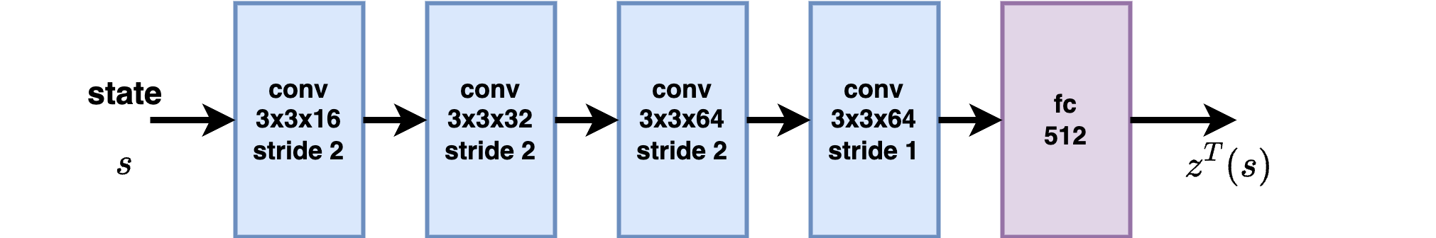
Figure 7: The target model architecture.

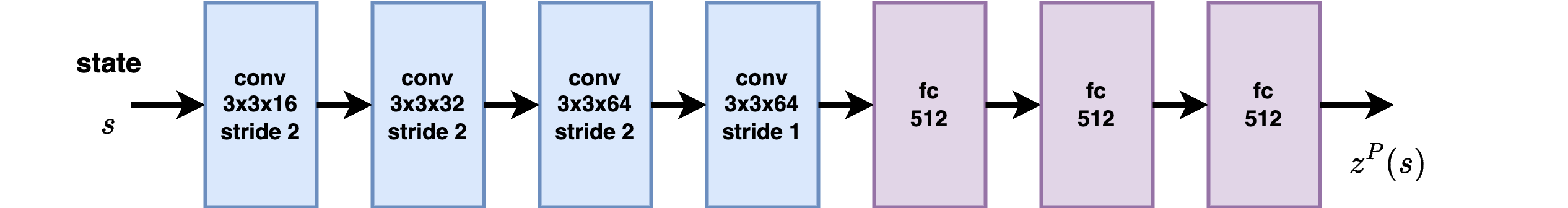
Figure 8: The predictor model architecture.

Table 1: Environment hyperparameters

Hyperparameter	Atari	Procgen
Observation downsampling	96$\times$96	64$\times$64
Frame stacking	4	2
State dimensionality for PPO	4$\times$96$\times$96	6$\times$64$\times$64
State dimensionality for IM modules	1$\times$96$\times$96	3$\times$64$\times$64
Parallel environments count	128	128
State normalisation	$s/255$	$s/255$
Samples per environment	1M	0.5M

Table 2: Agent hyperparameters

Hyperparameter	Value
PPO model learning rate	$0.0001$
Target model $\Phi^{\rm T}$ learning rate	$0.0001$
Predictor model $\Phi^{\rm P}$ learning rate	$0.0001$
Discount factor $\gamma^{\rm ext}$	$0.998$
Discount factor $\gamma^{\rm intr}$	$0.99$
Advantage external coefficient	$2.0$
Advantage intrinsic coefficient	$1.0$
Intrinsic reward scaling	$0.5$
Rollout length	$128$
Number of optimization epochs	$4$
Entropy coefficient	$0.001$
Epsilon clipping	$0.1$
Gradient norm clipping	$0.5$
GAE $\lambda$ coefficient	$0.95$
Optimizer	Adam
Weight initialisation	orthogonal, gain = $\sqrt{2}$

Table 3: Average cumulative reward (with standard deviation) per episode for all 3 preprocessing methods and maximal reward achieved by the agents, in case of Montezuma’s Revenge task.

Preprocessing method	Average reward	Max. reward
normalization	3.60 $\pm$ 0.14	7
mean subtraction	4.13 $\pm$ 0.12	7
none	2.31 $\pm$ 0.20	7

We followed [14] for setting the hyperparameters, to allow consistent comparison of results. We ran 128 parallel environments. For Atari, we used 1M samples for each environment (total 128M frames), for Procgen we used 0.5M samples for each environment (total 64M frames). The intrinsic motivation modules used no frame stacking, a single grayscale image for Atari environments and a single RGB image for Procgen.

The summary of all environment hyperparameters is in Table 1. The discount factors were set to $\gamma^{\rm ext}=0.998$ for external reward and $\gamma^{\rm intr}=0.99$ for intrinsic reward. The simulations revealed the importance of intrinsic reward scaling, the best result was achieved for $\eta=0.5$. The learning rate for all models was set to 0.0001. Actor and critic models used ReLU and motivation models worked best with ELU activation function. We also found that the deeper model with 3$\times$3 convolutions worked better than the standard Atari model using 8$\times$8 or 4$\times$4 convolutions in [33]. We retrained RND models to obtain comparable results and found faster convergence. The summary of PPO agent hyperparameters is in Table 2. More hyperparameters and further details of the learning process and the architectures of modules can be found in our source codes.

4.2 State preprocessing

The state before entering the motivation module of SND model can undergo preprocessing. We tested three preprocessing methods:

1. State normalization using the running mean and standard deviation,

2. Subtraction of the running mean value from the state,

3. No preprocessing.

We performed two training runs for each preprocessing method in 32M steps. For testing, we used SND-STD method. Table 3 demonstrates that the state preprocessing did not have a significant effect on agent performance (maximum reward achieved), only on the speed of learning. This also agrees with our assumption that operations such as subtraction of the mean or normalization should be able to find the network itself, trained using the self-supervised loss function. Therefore, it is not necessary for the designer to put them into the learning process explicitly. These conclusions will still need to be confirmed by statistical analysis. RND used mean subtraction and SND-V, SND-STD together with SND-VIC did not use input state preprocessing.

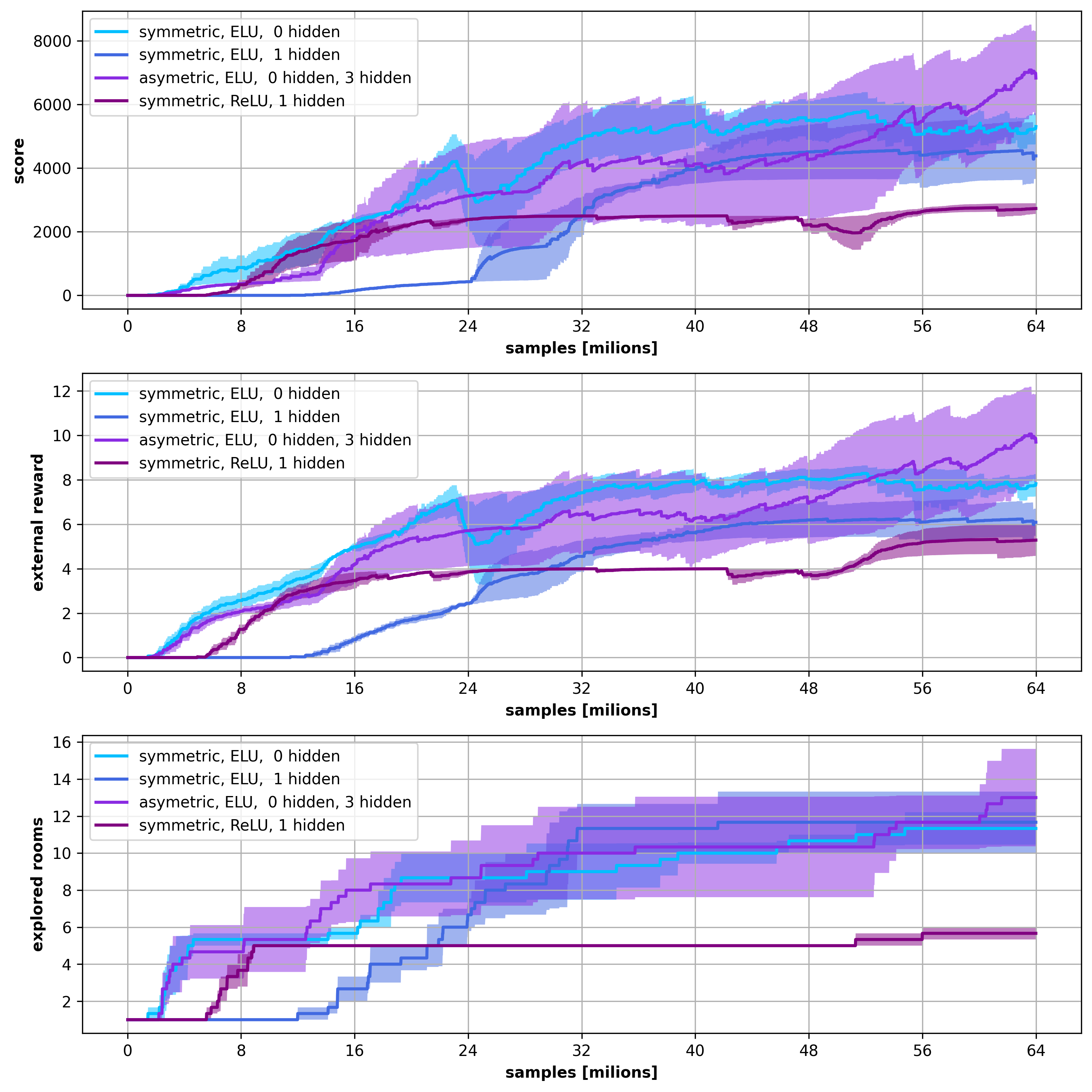
Figure 9: Agent performance based on various predictor model architectures, in case of Montezuma’s Revenge task, evaluated in terms of the overall score, external reward obtained and the number of rooms explored.

4.3 Results

We processed several quick experiments on Montezuma’s Revenge to explore an optimal setup. First we have to test the optimal architecture of $\Phi^{\rm T}$ and $\Phi^{\rm P}$ models. We experimented with 4 architectures:

1. identical models, one fully connected output layer, ELU activations

2. identical models, two fully connected layers, ELU activations

3. identical models, one fully connected layer, ReLU activations

4. asymmetric models, three fully connected layers for $\Phi^{\rm P}$, none for $\Phi^{\rm T}$, ELU activations fixed to fully connected convention.

Results of different model architectures are in Figure 9. The best result was achieved for the asymmetric architecture.

Next, we tested the effect of different augmentations. We considered three scenarios:

1. uniform noise, $\langle-0.2,0.2\rangle$

2. uniform noise, random tiles masking (tiles with sizes 1, 2, 4, 8, 12, 16)

3. uniform noise, random tiles masking, random convolution filter apply.

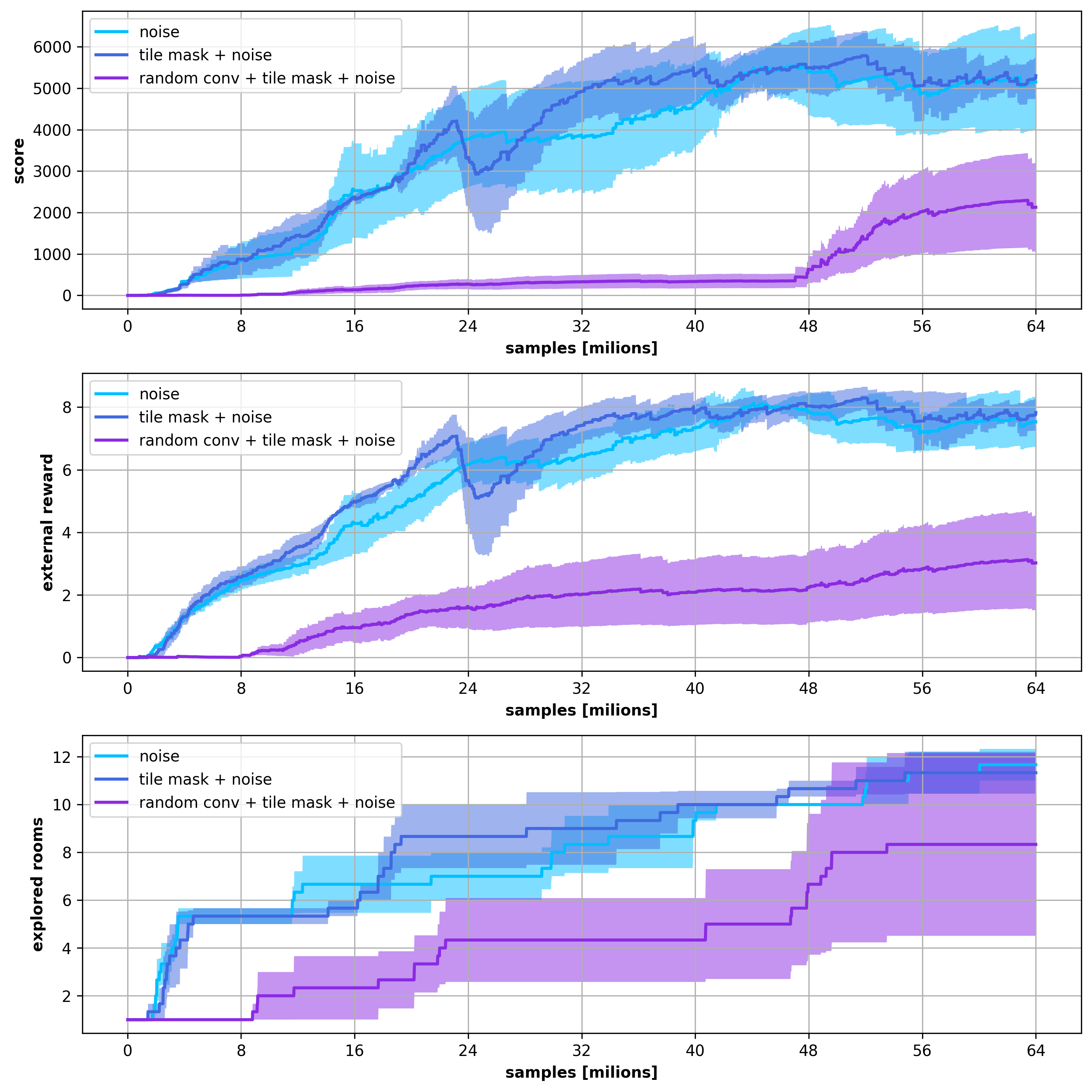
Figure 10: Agent performance for different state augmentations, in case of Montezuma’s Revenge task, evaluated in terms of the overall score, external reward obtained and the number of rooms explored.

Noise augmentation is commonly used in supervised image training. The tile masking forces the model to reconstruct incomplete information. Random convolution filter helps the model to learn to focus on informative features, not on texture colours. The results of different state augmentations are in Figure 10. We hypothesised that all three augmentations together would provide the best results. However, probably due to a shallow target model, this was not the case since the model was not able to learn sufficient transformation invariants. The best result was using uniform noise alone or with random tile masking as augmentations, in case of shallow target models.

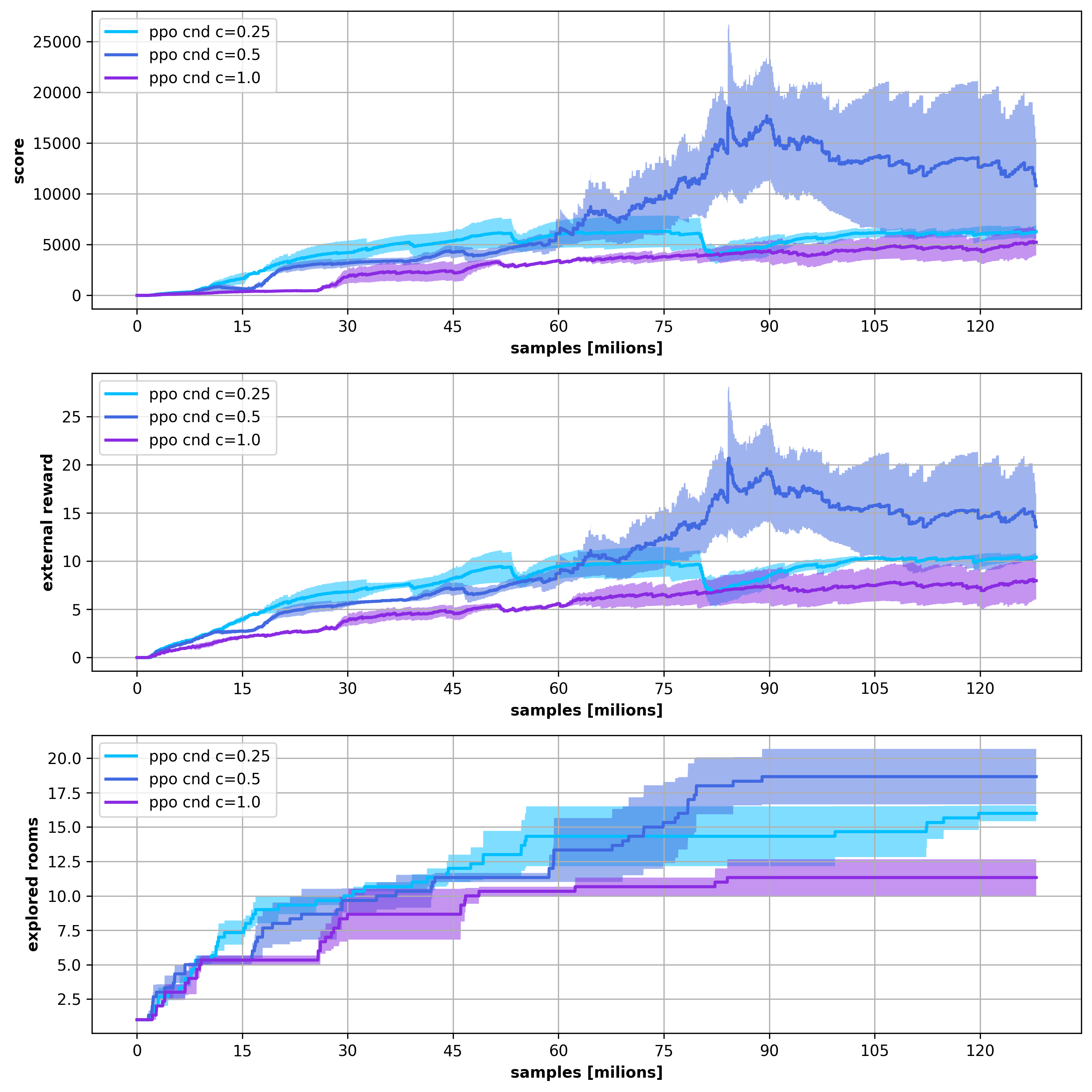
Figure 11: Agent performance for different intrinsic reward scaling methods, in case of Montezuma’s Revenge task, evaluated in terms of the overall score, external reward obtained and the number of rooms explored.

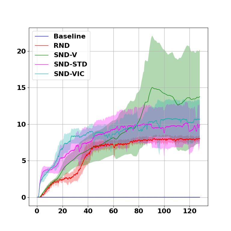
(a) Montezuma’s Revenge

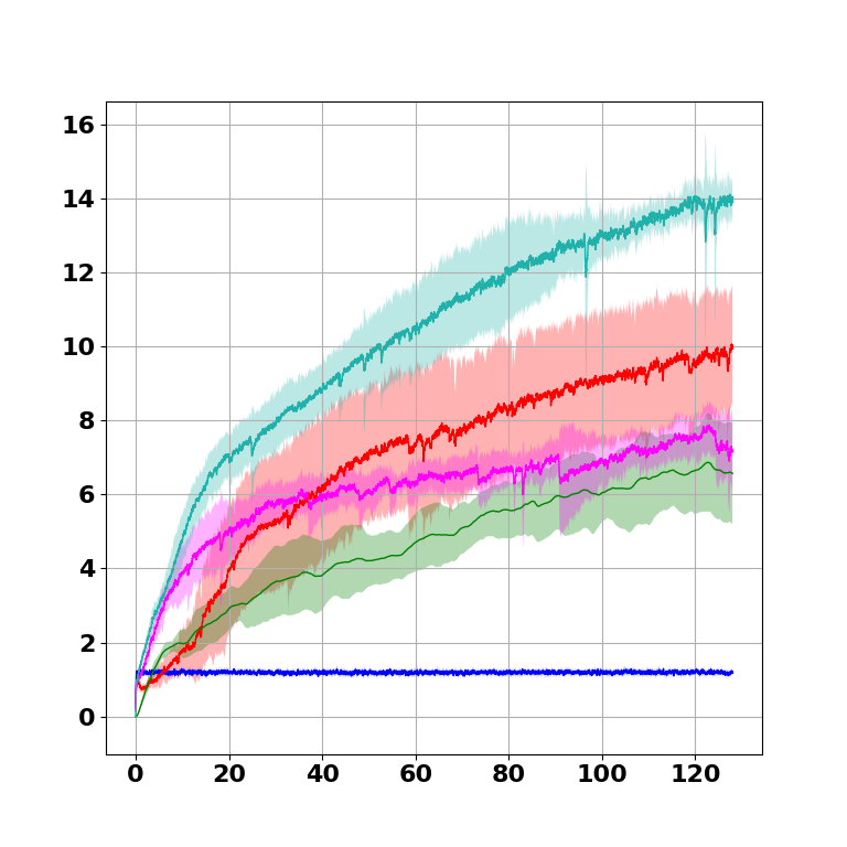
(b) Gravitar

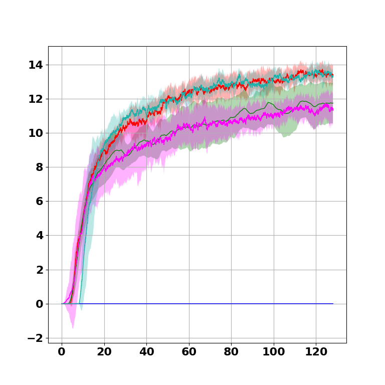
(c) Venture

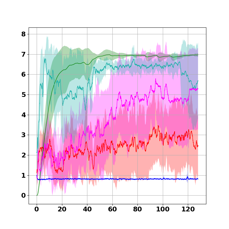
(d) Private Eye

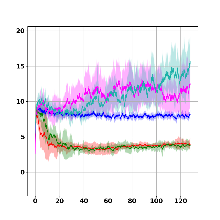
(e) Solaris

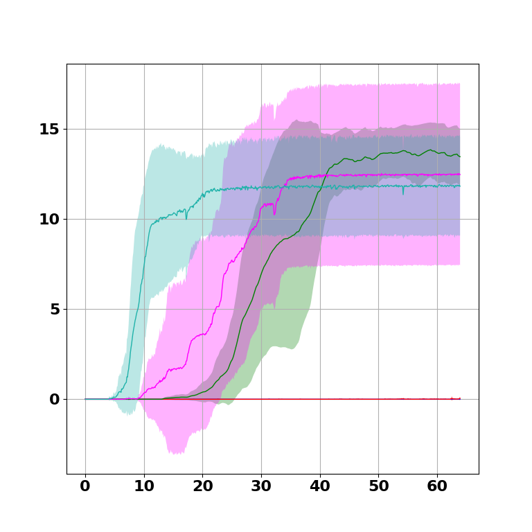
(f) Caveflyer

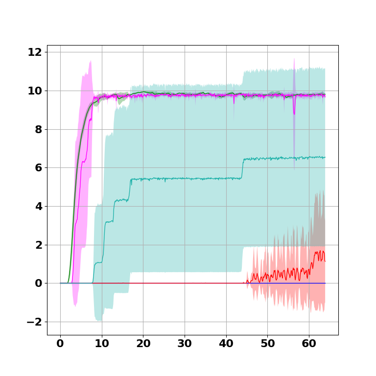
(g) Coinrun

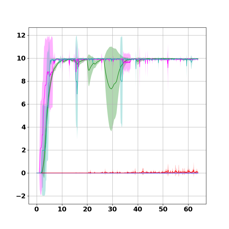
(h) Jumper

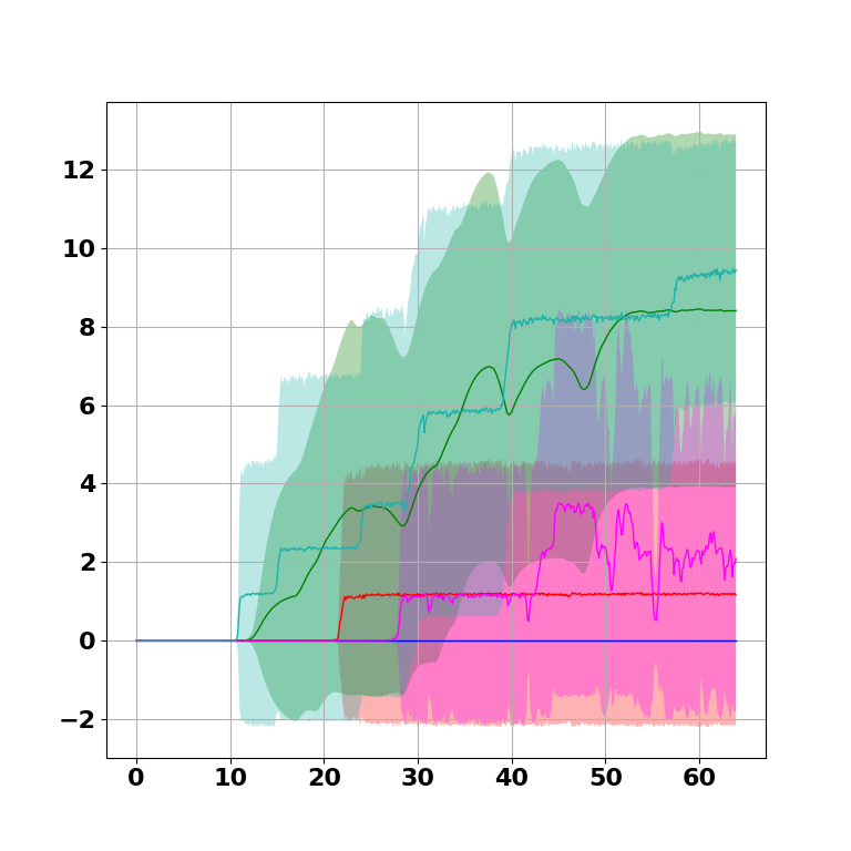
(i) Climber

Figure 12: The cumulative external reward per episode (with the standard deviation) received by the agent from the tested environment. We omitted the graph for the Pitfall environment, where all algorithms were not successful, having achieved zero reward. The horizontal axis shows the number of steps in millions, the vertical axis refers to the external reward.

Table 4: Average cumulative external reward per episode for tested models. The best models for each environment are shown in bold face.

	Baseline	RND	SND-V	SND-STD	SND-VIC
Montezuma	0.00 $\pm$ 0.00	5.33 $\pm$ 0.23	8.87 $\pm$ 2.79	7.76 $\pm$ 1.73	8.45 $\pm$ 1.12
Gravitar	1.19 $\pm$ 0.00	6.63 $\pm$ 1.55	4.73 $\pm$ 0.61	5.89 $\pm$ 0.43	10.05 $\pm$ 0.66
Venture	0.00 $\pm$ 0.00	11.18 $\pm$ 0.42	9.71 $\pm$ 0.97	9.54 $\pm$ 0.90	11.36 $\pm$ 0.37
Private Eye	0.81 $\pm$ 0.01	2.41 $\pm$ 0.95	6.44 $\pm$ 0.27	3.79 $\pm$ 1.24	5.93 $\pm$ 0.47
Pitfall	0.00 $\pm$ 0.00	0.00 $\pm$ 0.00	0.00 $\pm$ 0.00	0.00 $\pm$ 0.00	0.00 $\pm$ 0.00
Solaris	8.08 $\pm$ 0.15	3.84 $\pm$ 0.25	3.96 $\pm$ 0.41	11.61 $\pm$ 1.12	10.85 $\pm$ 1.20
Caveflyer	0.00 $\pm$ 0.00	0.00 $\pm$ 0.00	7.28 $\pm$ 1.62	10.86 $\pm$ 4.37	11.14 $\pm$ 2.35
Coinrun	0.00 $\pm$ 0.00	0.25 $\pm$ 0.50	9.40 $\pm$ 0.05	9.40 $\pm$ 0.07	2.55 $\pm$ 3.63
Jumper	0.00 $\pm$ 0.00	0.03 $\pm$ 0.02	9.22 $\pm$ 0.21	9.76 $\pm$ 0.04	9.76 $\pm$ 0.03
Climber	0.00 $\pm$ 0.00	1.00 $\pm$ 2.83	4.63 $\pm$ 2.96	1.48 $\pm$ 2.40	6.62 $\pm$ 3.24

Table 5: Results of two-sided nonparametric Mann-Whitney U tests on selected pairs of models.

Environment	Method	Method	U statistic	$p$-value
Montezuma	SND-V	SND-STD	45.00	0.42
	SND-V	SND-VIC	38.00	0.89
	SND-STD	SND-VIC	25.00	0.51
Venture	RND	SND-VIC	27.00	0.42
Private Eye	SND-V	SND-VIC	63.00	0.01
Solaris	SND-STD	SND-VIC	34.00	0.88
Caveflyer	SND-STD	SND-VIC	40.00	1.00
Coinrun	SND-V	SND-STD	14.00	1.00
Jumper	SND-V	SND-STD	0.00	0.01
	SND-V	SND-VIC	0.00	0.04
	SND-STD	SND-VIC	25.00	0.80

Table 6: Average maximal score reached by tested models on Atari environments. The best model for each environment is shown in bold face.

	Baseline	RND	SND-V	SND-STD	SND-VIC
Montezuma	400	6689	14973	7212	7838
Gravitar	2611	5600	2469	4643	6712
Venture	22	2167	1661	2138	2188
Private Eye	14870	14996	4438	15089	17313
Pitfall	0	0	0	0	0
Solaris	12344	10667	11582	12460	11865

Finally, we tested an intrinsic reward scaling. Low value can lead to stacking the agent into a non-exploring policy. High value can prevent the agent from collecting extrinsic rewards, or make it too sensitive to small unimportant changes, both causing instability. We tested three values: 0.25, 0.5 and 1.0. Figure 11 shows that the best score is achieved with 0.5 reward scaling value. However, some environments provide better results after fine-tuning to 0.25. Figure 12 captures the cumulative external reward per episode and the standard deviation of the tested models in 9 different environments.

Table 4 provides the overall average results on tested models in 10 environments. It is evident from visual inspection that our SND models excel in the case of all but one environment. For each environment, the best models (with the highest average score) are shown in bold to facilitate orientation (as explained below). In order to get a statistically more accurate view of the results, we applied statistical tests that we found meaningful in case of our data. Based on a smaller number of (time intensive) runs (8-9) for each environment and the model, and large differences between models (in most cases) we applied paired non-parametric Mann-Whitney U tests for models with similar (top) performance to test significance of differences. The results shown in Table 5, provide a $p$-value for each paired test. Higher $p$-values indicate that in most environments (Montezuma, Venture, Solaris, Caveflyer, Coinrun, Jumper) the top performing models were statistically indifferent (and hence are all shown in bold in Table 4).

Table 6 shows the maximum achieved score for Atari environments which is often used for model comparison (although we would like to emphasize that the agent never receives this score as a reward, and therefore it is not its goal to maximize it). The best results were achieved with the models based on SND motivation, while in 8 cases it was with a significant lead over the existing algorithms (in Venture environment the results were almost the same as those of the RND model). When evaluating the score, the SND models achieved the highest score in 5 Atari environments (with the exception of the already mentioned Pitfall) and in 3 cases (Montezuma’s Revenge, Gravitar, Private Eye) it was significantly higher than the compared models.

In Venture enviroment, the RND model scores comparably to the best SND-VIC model. the reason could be that all SND agents fall into a “repetitive reward trap”: the agent quickly learns to enter one room, collect points, and after exiting, enter again where points can be collected again by the same policy. Pitfall environment looks most challenging, due to extremely sparse rewards, which probably led to complete failure of all models. It contains very similar rooms, where the noise dominates - as NPC creatures blink or randomly move, which misleads the agents into focusing on noise as novelty.

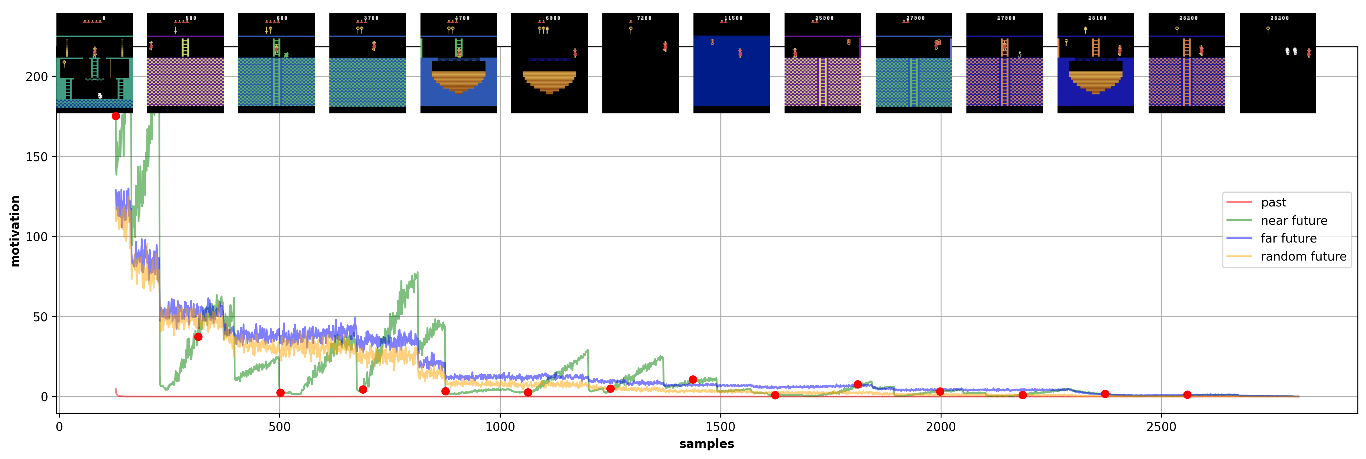
(a) RND

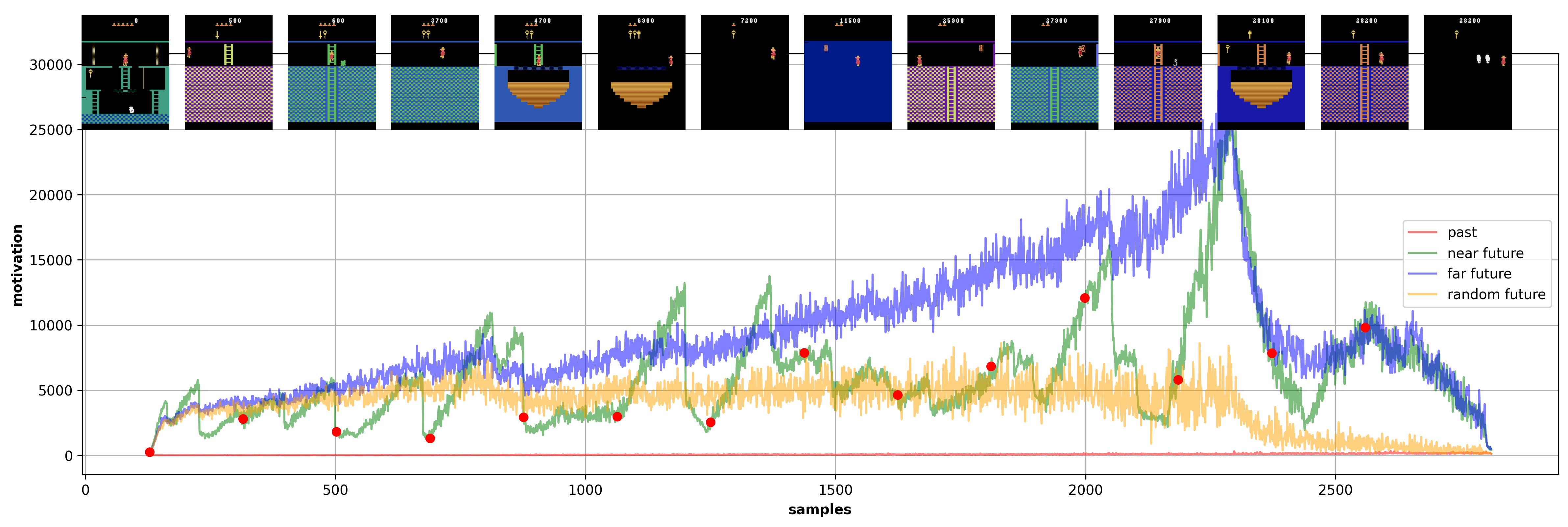
(b) SND-STD

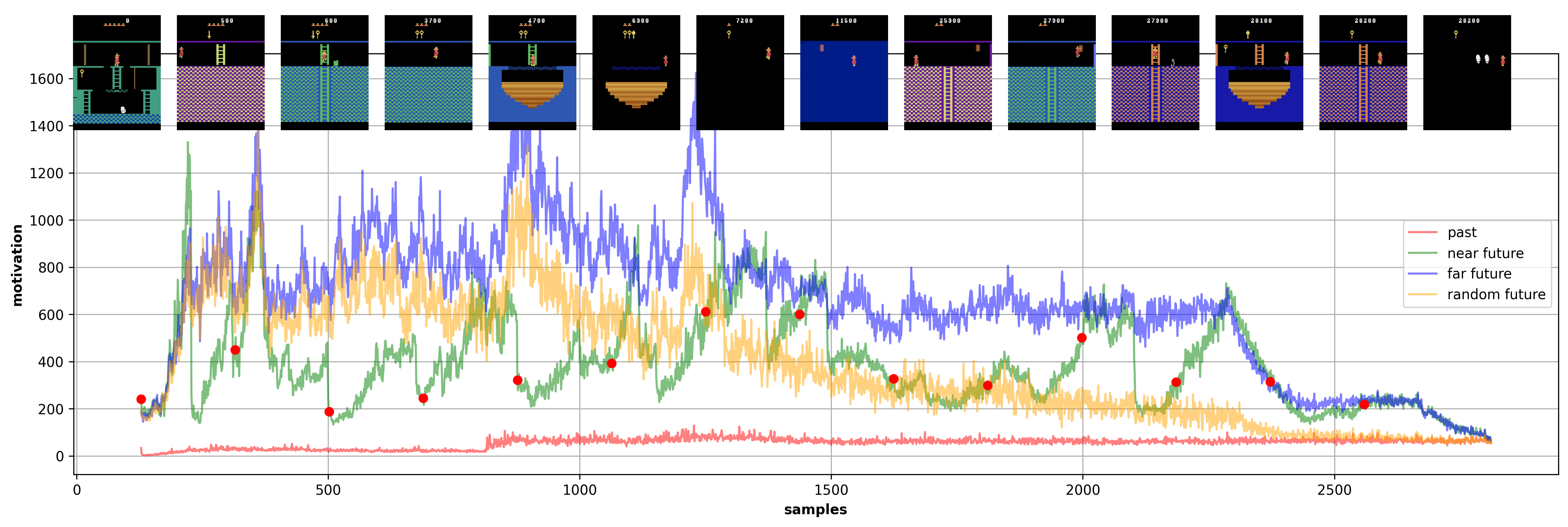
(c) SND-V

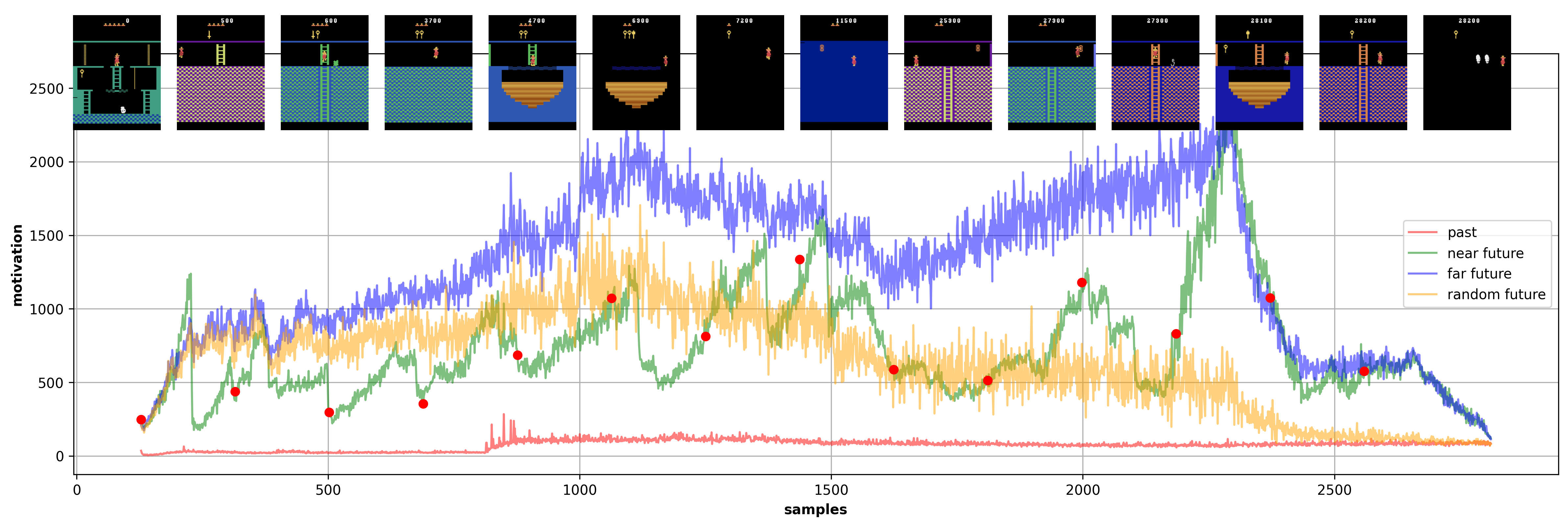
(d) SND-VIC

Figure 13: Novelty detection for different regularisation losses as a reaction to different future windows. The states were collected on Montezuma’s Revenge with our best agent, red dots correspond to state examples shown above.

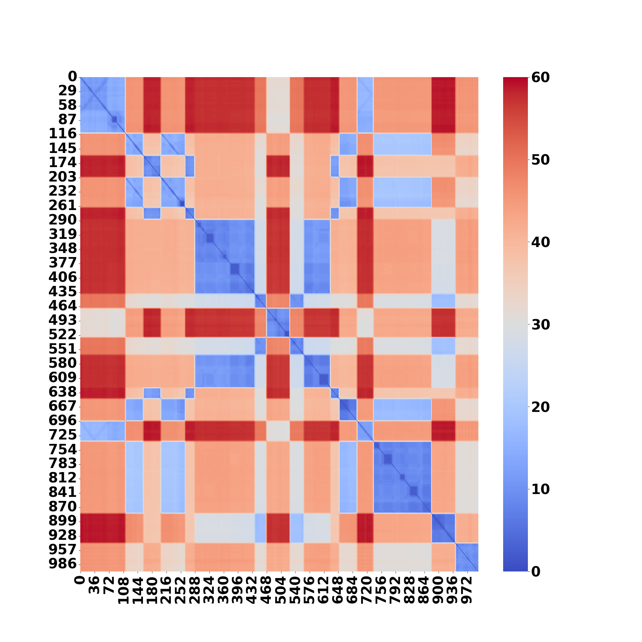
(a) States

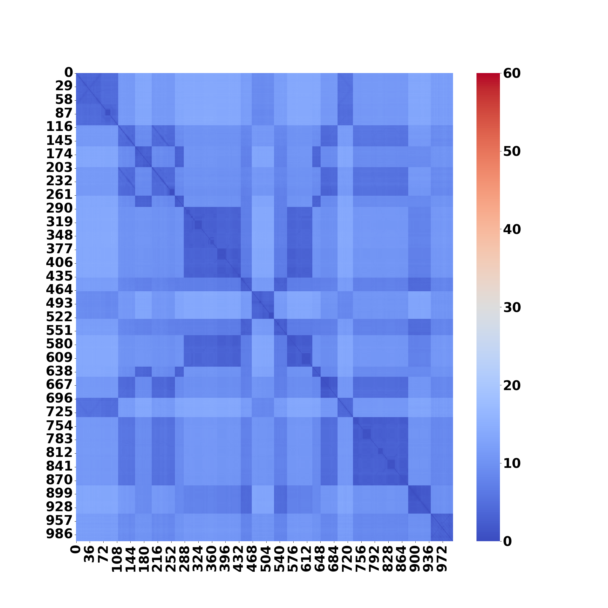
(b) RND

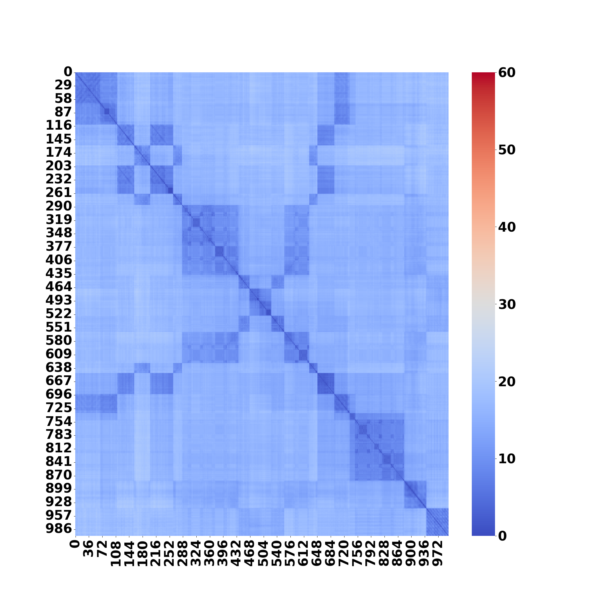
(c) SND-STD

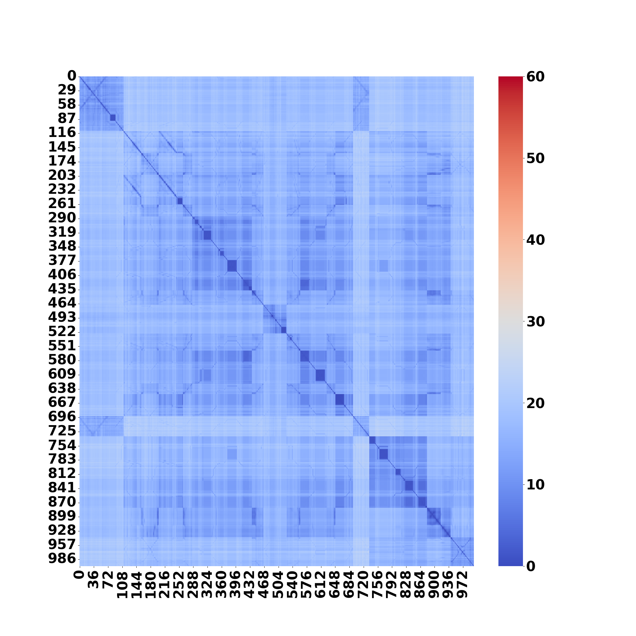
(d) SND-V

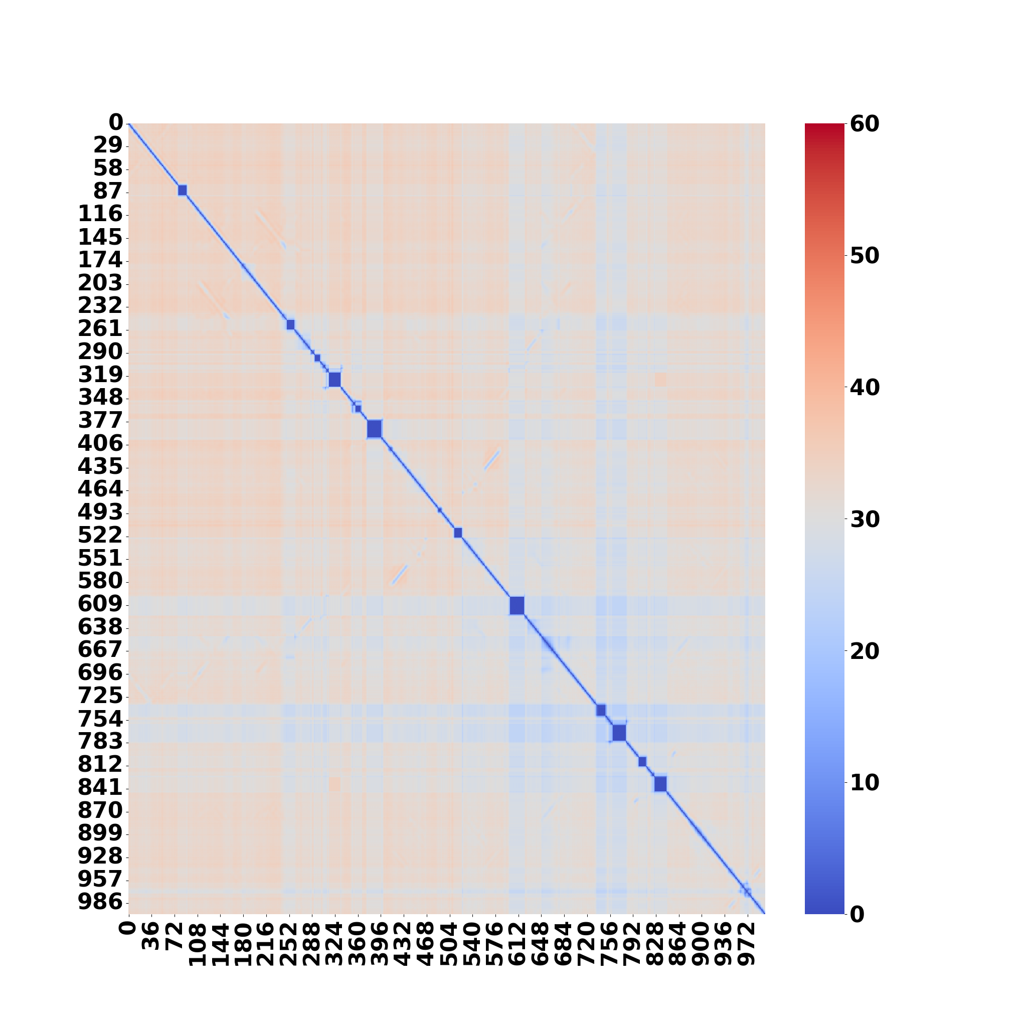
(e) SND-VIC

Figure 14: The distance matrix of 1000 states and the feature vectors collected from Montezuma’s Revenge environment. Small distances are displayed in blue colour, while large distances are displayed in red colour.

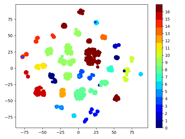
(a) Random target model

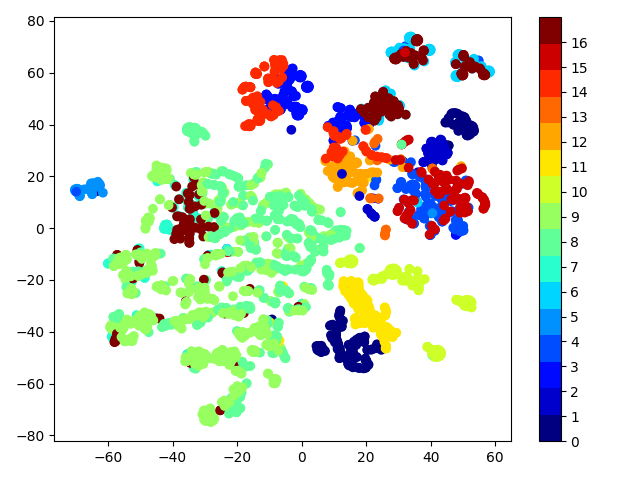
(b) Trained target model

Figure 15: The t-SNE projected feature representations of the target model in Montezuma’s Revenge task. The colours correspond to different rooms.

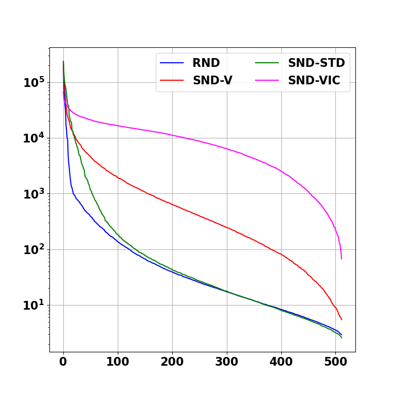
(a) Montezuma’s Revenge

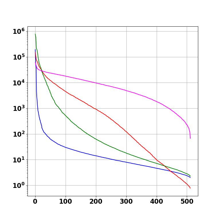
(b) Gravitar

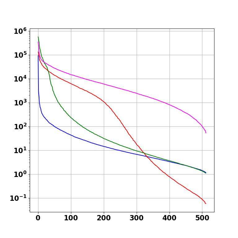
(c) Venture

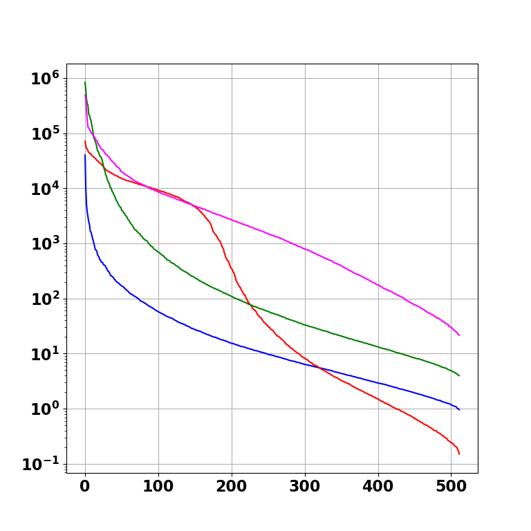
(d) Private Eye

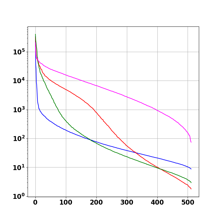
(e) Solaris

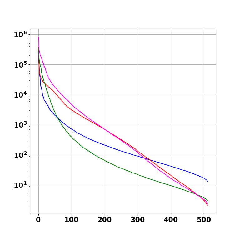
(f) Caveflyer

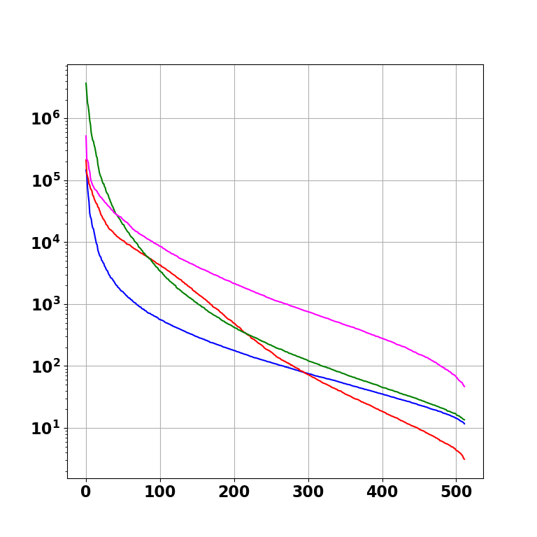
(g) Coinrun

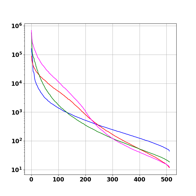
(h) Jumper

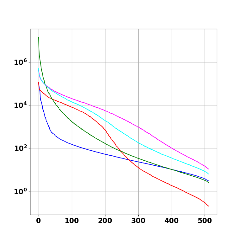
(i) Climber

Figure 16: Descendingly ordered eigenvalues of a linear envelope obtained using the PCA method, which show the stretching of the feature space in individual dimensions. The horizontal axis denotes the indices of eigenvalues, the vertical axis shows the magnitude of eigenvalue on a logarithmic scale. Based on these data, we aimed to find out if there is a connection between the shape of the feature space and the performance of the given model. The graph for Pitfall was omitted since it looked very similar to Private Eye.

Table 7: Description of the target model feature space created by four selected methods. For the evaluation, we used the following parameters: mean value and standard deviation of the $L_{2}$-norm of features, 25th, 50th, 75th, and 95th percentiles of eigenvalues of a linear envelop to obtain a rough representation of stretching of the feature space in individual dimensions. To this, we add the maximum achieved external reward ($\max(r_{\rm ext})$), so that it is possible to search for a connection between the parameters of the feature space and the performance of the method.

Environment	Method	$\max({r_{\rm ext}})$	$L_{2}$-norm	$Q_{25}$	$Q_{50}$	$Q_{75}$	$Q_{95}$
Montezuma	RND	9	1.93 $\pm$ 1.15	9	24	89	778
	SND-STD	16	4.85 $\pm$ 2.45	9	26	109	6835
	SND-VIC	17	6.22 $\pm$ 2.99	3066	8429	14858	25634
	SND-V	34	6.41 $\pm$ 3.96	98	378	1367	8944
Gravitar	SND-V	9	11.94 $\pm$ 3.81	16	341	2919	24291
	SND-STD	15	11.66 $\pm$ 2.82	8	30	250	20402
	RND	20	1.12 $\pm$ 0.81	5	10	24	139
	SND-VIC	21	7.26 $\pm$ 3.01	2263	6837	15173	27908
Private Eye	SND-V	7	15.47 $\pm$ 6.50	2	27	6801	23823
	RND	9	1.40 $\pm$ 0.65	3	9	37	410
	SND-STD	9	8.03 $\pm$ 4.46	15	54	371	24025
	SND-VIC	10	4.29 $\pm$ 3.56	232	1401	6197	47342
Pitfall	RND	0	1.31 $\pm$ 0.39	3	10	47	410
	SND-V	0	2.81 $\pm$ 1.43	2	124	7358	27402
	SND-STD	0	10.64 $\pm$ 2.81	8	32	319	39904
	SND-VIC	0	5.62 $\pm$ 1.79	153	1542	9827	44126
Venture	SND-V	14	3.67 $\pm$ 3.07	1	130	3921	24443
	RND	18	0.68 $\pm$ 0.80	4	9	30	188
	SND-STD	18	4.50 $\pm$ 3.79	4	15	115	32272
	SND-VIC	18	4.91 $\pm$ 3.89	1006	3644	11256	41899
Solaris	RND	55	3.68 $\pm$ 3.42	29	62	172	776
	SND-V	65	10.19 $\pm$ 6.39	13	165	3337	18085
	SND-STD	81	5.77 $\pm$ 4.28	12	37	211	11171
	SND-VIC	87	6.00 $\pm$ 4.14	1649	5079	13163	32377
Caveflyer	RND	10	5.06 $\pm$ 2.98	48	128	474	4792
	SND-V	16	10.35 $\pm$ 8.37	28	293	2007	20416
	SND-STD	16	9.69 $\pm$ 5.90	11	34	206	13452
	SND-VIC	16	9.89 $\pm$ 5.70	23	271	2638	49517
Climber	RND	0	7.47 $\pm$ 3.53	12	32	106	1500
	SND-V	11	17.31 $\pm$ 6.45	2	53	5091	25463
	SND-STD	11	48.56 $\pm$ 22.16	12	63	788	49506
	SND-VIC	11	13.41 $\pm$ 4.01	144	2313	14132	78074
Coinrun	RND	10	5.07 $\pm$ 3.00	40	109	389	4029
	SND-V	10	12.02 $\pm$ 7.20	23	149	2473	21553
	SND-STD	10	29.23 $\pm$ 17.06	54	200	1651	76730
	SND-VIC	10	11.23 $\pm$ 5.77	332	1140	5414	44014
Jumper	RND	10	8.63 $\pm$ 2.19	139	337	1008	6733
	SND-V	10	14.97 $\pm$ 5.49	63	314	3310	20896
	SND-STD	10	15.51 $\pm$ 3.73	61	189	1044	22008
	SND-VIC	10	20.79 $\pm$ 6.18	47	257	6271	74860

4.4 Analysis of results

We analyzed the results using three different methods in a reasonable order. The first method compares the models from the view of the quality of an intrinsic reward acquired during training. The second approach focuses on the distribution of the representations in the feature space and shows how the distances of points in the state space are transformed in the feature space. The third approach contains the spatial analysis of the features spaces based on computing eigenvalues of the linear envelope of the feature space.

4.4.1 Quality of an intrinsic reward

By means of the first analysis we want to demonstrate that the presented results were achieved thanks to a better intrinsic reward signal which is superior to the signal of RND method. For different regularisation losses, we wanted to understand its time evaluation and show the ability to provide a large IM signal for previously unseen states. For the purpose of exploration, the most important is the ability to detect near future states which are very close to already seen ones. We collected a set of 2700 states from our best agent playing Montezuma’s Revenge. During the experiment, we trained the IM modules only on past data and tested them on future data. The testing batch was selected from the following 4-time horizons, with respect to the agent being in step $n$, and testing batch indices $m$:

1. past: already seen states, $m<n$

2. near future: $n<m<n+128$ steps in the future

3. far future: $m>n$

4. random: any batch from the set

We hypothesised that the Random Network distillation would provide a sufficient signal only at the beginning of learning. Convergence to zero leads to limited exploration abilities. This degradation corresponds to our results in Figure 13(a). On the other hand, continuously updated target models can provide useful signals for the entire run. The corresponding results are displayed in Figures 13(b)–d. On all three losses, the intrinsic motivation is much higher for unseen states, and not converging into zero. The strong peaks for the near future correspond to new rooms finding. The self-supervised regularisation prevents collapsing the motivation signal to zero. This insight implies requirements for an exploration signal. For future research, this also provides a simple methodology for testing exploration abilities, without training the whole RL agent, which can be time-consuming.

4.4.2 Distribution of the representations in the feature spaces

In the second analysis, we investigated how the distances of points in the state space are mapped to the feature space. For a better idea of how the SND methods work, we visualized the feature space by collecting 1000 states in Montezuma’s Revenge environment from a trained agent and calculating their distance matrix. Figure 14 illustrates how much of the structure of the state space is preserved and transferred to the feature space. The patterns on the diagonal correspond to individual rooms in the environment where the states are similar to each other and therefore their mutual distance is small (blue colour), while the distances to the states from other rooms are large (red colour). One can notice that in the case of both RND and SND-STD, a similar structure of distances is preserved as in the case of states, but with smaller differences. When comparing RND and SND-STD with each other, it can be seen that the feature vectors created by the SND-STD method still have larger distances, which is indicated by the light blue colour. In contrast, the SND-V method did not preserve the original structure of the state space, although some fragments can be seen there that can be mapped to the input data. In any case, it can be seen that initially, similar states are significantly further apart in this space. Finally, SND-VIC is extremely contrastive and apart from the main diagonal, there is no distinct original structure. However, the light red colour indicates that the distances for almost any state are larger than the three previous methods, which indicates better discriminative capabilities of SND-VIC. The enhanced discriminative capabilities of SND methods can explain more efficient novelty detection that provides a better intrinsic reward signal.

To demonstrate the described property, we can visualise the learned feature vectors $Z$ in 2D using t-SNE method [54]. Figure 15 shows the resulting features of the trained target model on Atari Montezuma’s Revenge task. The randomly initialised trained network (the same as in [14], Figure 15(a)) can differentiate well between different rooms, however within the room the variance is low, pointing to the lack of exploration abilities. On the other hand, the self-supervised regularized target model in Figure 15 provides a much larger variance of features, which provides a more sensitive novelty detection signal.

4.4.3 Spatial analysis of the feature spaces

The main goal of the third analysis was to find out the differences (not only visually) among the individual spaces of features, to describe them with some quantities and to find a possible connection to the performance of the algorithm and the mentioned quantities. From the set of examined models for one environment, we always selected the model with the highest obtained reward and generated 10,000 samples of input states by running it in the environment. Subsequently, each model generated feature vectors for a sample of previously collected input states. Hence, we obtained feature space samples $Z$ of each model. Using principal component analysis (PCA) we found the linear envelope of the high-dimensional manifold that forms the feature space. We examined the mean value and especially the variance of the feature vectors, and also the eigenvalues using PCA, which indicate the basic shape of the feature space (i.e. the sizes of the individual dimensions).

The results of this analysis are shown in Figure 16 and Table 7. For the evaluation, we decided to use the following parameters: mean value and standard deviation of the $L_{2}$-norm of features, 25th, 50th, 75th and 95th percentiles of eigenvalues to obtain a rough representation of stretching of the feature space in individual dimensions. It can be seen that in almost all cases the RND target model has smaller eigenvalues than the SND models. This is also evident for the $L_{2}$-norm values that the entire RND feature space has a smaller volume compared to the SND feature space. On the other hand, RND and SND-STD are similar in shape. Their curves have a convex shape, with SND-STD having more stretched dimensions. SND-V and SND-VIC also have similarly concave shapes, but SND-V stretches only about half of the available dimensions and then usually falls more steeply. The shape of the SND-VIC curve is ensured by the variance (Eq. 12) and covariance (Eq. 13) components of its loss function. The missing decorrelation term in the SND-V loss function (Eq. 5) results in an uneven stretching of the dimensions.

In contrast, the shape of the SND-STD curve is convex and the dimensions are used unevenly. After these analyses, we tried to improve the variance within the dimensions by adding a regularization term (Eq. 10) which tried to maximize the variance within the feature vector. However, such a term had an expansive effect on the feature space and it was not possible to give it much weight, because the loss function (Eq. 8) of the ST-DIM algorithm has an expansive effect and the addition of another expansive term led to problems with the uncontrolled expansion of the feature space. Despite the small influence of the variance component of the loss function, the performance of SND-STD improved and it helped prevent agents from getting stuck in certain cases. If we compare RND and SND-STD feature spaces (in terms of eigenvalues) they look similar, but the latter model was able to achieve better results in 7 out of 9 environments. Our findings show that when training the target model, it is important to enforce the decorrelation of features and the equal use of all dimensions of the feature space. Such a model seems to be relatively robust and sufficiently sensitive to novelty.

Interestingly, for the Pitfall task (not shown in Figure 16), despite their failure, our methods still tried to take advantage of the feature space dimensions. From the analysis of the trained agents, we saw that they were able to explore several rooms, but in each, there were enough moving objects that made the given state space rich and thus made it difficult to train the predictor model. This led to a very slow decrease in the intrinsic reward (we observed a similar behaviour after short training sessions in other environments). We assume that with a larger number of training steps, the agent would eventually be able to reach the reward.

5 Discussion

At the beginning, we asked ourselves the following questions: Are the features provided by the original RND target model sufficient? Can the model learn better features? In the paper Random Network Distillation [14], the orthogonal weight initialization method was used to set the parameters of the target model and distribute its representations over the state space, which provides a sustainable intrinsic reward. We assumed that if it is possible to find suitable algorithms for training the target model, it will also be possible to improve the results of the RND model. Based on these considerations, we proposed a number of SND methods.

The methods worked very well in most cases, so in the analysis, we focused on their deeper understanding. First, we used a geometric approach trying to capture, at least in rough outlines, the properties of feature spaces. A comparison between a randomly initialized feature space and a feature space formed using one of the SND algorithms supports the correctness of our assumptions that self-supervised algorithms can distinguish even subtle differences within the state space. This turned out to be one of the weaknesses of the RND algorithm which, while being good at differentiating between sufficiently different states (e.g. different rooms in Montezuma’s Revenge), was placing similar states close to each other in the feature space, making the work of the predictor model easier. In the experiments, we thus observed a decrease in the standard deviation of the average intrinsic reward per episode, which meant that most of the visited states generated a similar reward.

Last but not least, we performed an analysis of novelty detection abilities of selected methods. After comparison with RND as a baseline, we can conclude that this baseline suffers from an IM-based reward vanishing problem. After adding the regularisation to the target model, much better features were obtained with a significant change compared to the baseline. Intrinsic reward vanishing disappears for all the tested losses. This is cross-validated also on t-SNE features visualisation, where regularised features yield much higher variance, which means larger sensitivity to novelty.

We experimented with different target model architectures, different augmentations and intrinsic reward scaling. We found that what worked best was the target model using ELU activation function and only one fully connected layer, and the predictor model having three hidden layers. From the tested augmentations (noise, random tile masking, random convectional filter) we found the best performance for a combination of uniform noise with random tiles masking. As a questionable augmentation remains random downsampling and upsampling back, which could help remove noise while preserving representative information in the state vectors. We suggest investigating this idea for the next research. The scaling of an intrinsic reward reveals a large sensitivity of the model to this hyperparameter. The best working value was 0.5, but we think that this value should be optimized separately for each specific environment.

We did not specifically investigate the robustness of SND methods concerning the initialization of the target model (which was again a problem with RND). We assume that self-supervised learning algorithms can cope with a poorly initialized model to a certain extent, but from the training experience, we found that it is better to initialize the target models of SND-STD and SND-VIC to small values ($gain=0.5$) and let it expand itself while SND-V was initialized like RND to higher values ($gain=\sqrt{2}$).

Our experiments have shown that if the ST-DIM algorithm works on an incomplete dataset that takes on new samples (the authors probably did not test it in such conditions), there is instability and an exponential increase of activity in the feature space at certain moments. This is related to the use of a cross-entropy loss function in its core (which does not limit the values of inputs – logits) where derivatives can reach large values and subsequently inflate the entire feature space.

During the development of the model, we found that it is best to minimize the $L_{2}$-norm of logits that enter the cross-entropy. We also tried to maximize the entropy of the distributions generating the respective logits and minimize the $L_{2}$-norm of global features, but both approaches failed to sufficiently stabilize the algorithm. As another thing, we investigated the effect of state preprocessing on the performance of the SND-STD model, but it had no significant effect on the agent performance.

A direct extension of SND methods will be the merging of the target model with the model to which the actor and critic are connected. We have already done some pilot research in this direction and it seems to be a feasible task. This would greatly optimize the entire model and speed up its training in terms of computing time.

The SND methods provide room for experimenting with other suitable algorithms for training the target model. Since none of our three tested methods proved universally superior (i.e. that it would beat the others in all environments), it can be concluded that different environments require slightly different representations of the target model. On the positive side, we first optimised these methods in the Atari environments and were then able to port them to ProcGen with minimal fine-tuning, immediately achieving very good results.

At the same time, we think that this approach can be an inspiration for a new class of algorithms that will specialize in creating feature mapping capturing the relationship of the environment to the agent itself since current self-supervised methods are agnostic to these relationships.

6 Conclusion

In this work, we presented novel methods based on Self-Supervised Network Distillation (SND) that can help solve tasks in sparse reward environments using an intrinsic motivation signal. The main idea of SND is to distill knowledge from the target model using the predictor model, while the target model builds its state representations using self-supervised algorithms. The difference between the representations of the target model and the predictor model serves as a motivational signal. We adapted three existing self-supervised algorithms for training the target model and tested them experimentally on a set of environments that are considered difficult to explore. The SND methods are a generalization of the RND method based on the novelty detection approach where the target model is randomized and fixed. Three analytical methods we used revealed the weaknesses of the RND approach – the need for good initialization, the low variance of intrinsic reward in different states, and the loss of the motivational signal due to the adaptation of the predictor model. Through empirical experiments, we were able to demonstrate the superior performance of the SND methods over our baseline and RND agents in different game environments. This highlights the effectiveness and versatility of the SND methods for improving learning in sparse reward scenarios and demonstrates their potential as a valuable tool for reinforcement learning applications.

References

- Agarwal et al., [2021] Agarwal, R., Schwarzer, M., Castro, P. S., Courville, A. C., and Bellemare, M. (2021). Deep reinforcement learning at the edge of the statistical precipice. In Advances in Neural Information Processing Systems, volume 34, pages 29304–29320.
- Anand et al., [2019] Anand, A., Racah, E., Ozair, S., Bengio, Y., Côté, M., and Hjelm, R. D. (2019). Unsupervised state representation learning in Atari. CoRR, abs/1906.08226.
- Assran et al., [2022] Assran, M., Caron, M., Misra, I., Bojanowski, P., Bordes, F., Vincent, P., Joulin, A., Rabbat, M., and Ballas, N. (2022). Masked Siamese networks for label-efficient learning. arXiv e-prints, page arXiv:2204.07141.
- Aubret et al., [2019] Aubret, A., Matignon, L., and Hassas, S. (2019). A survey on intrinsic motivation in reinforcement learning. arXiv preprint arXiv:1908.06976.
- Aubret et al., [2023] Aubret, A., Matignon, L., and Hassas, S. (2023). An information-theoretic perspective on intrinsic motivation in reinforcement learning: A survey. Entropy, 25.
- Badia et al., [2020] Badia, A. P., Sprechmann, P., Vitvitskyi, A., Guo, D., Piot, B., Kapturowski, S., Tieleman, O., Arjovsky, M., Pritzel, A., Bolt, A., et al. (2020). Never give up: Learning directed exploration strategies. arXiv:2002.06038.
- Baldassarre, [2019] Baldassarre, G. (2019). Intrinsic motivations and open-ended learning. arXiv:1912.13263v1 [cs.AI].
- Baldassarre et al., [2014] Baldassarre, G., Stafford, T., Mirolli, M., Redgrave, P., Ryan, R. M., and Barto, A. (2014). Intrinsic motivations and open-ended development in animals, humans, and robots: An overview. Frontiers in Psychology.
- Bardes et al., [2022] Bardes, A., Ponce, J., and LeCun, Y. (2022). VICReg: Variance-invariance-covariance regularization for self-supervised learning. In International Conference on Learning Representations.
- Barto, [2013] Barto, A. (2013). Intrinsic Motivation and Reinforcement learning, page 17–47. Springer, Berlin/Heidelberg, Germany.
- Barto and Simsek, [2005] Barto, A. G. and Simsek, O. (2005). Intrinsic motivation for reinforcement learning systems. In Proceedings of the 13th Yale Workshop on Adaptive and Learning Systems, pages 113–118. Yale University Press.
- Bellemare et al., [2013] Bellemare, M. G., Naddaf, Y., Veness, J., and Bowling, M. (2013). The arcade learning environment: An evaluation platform for general agents. Journal of Artificial Intelligence Research, 47:253–279.
- [13] Burda, Y., Edwards, H., Pathak, D., Storkey, A., Darrell, T., and Efros, A. A. (2018a). Large-scale study of curiosity-driven learning. arXiv:1808.04355.
- [14] Burda, Y., Edwards, H., Storkey, A., and Klimov, O. (2018b). Exploration by random network distillation. arXiv:1810.12894.
- Chopra et al., [2005] Chopra, S., Hadsell, R., and LeCun, Y. (2005). Learning a similarity metric discriminatively, with application to face verification. In IEEE Computer Society Conference on Computer Vision and Pattern Recognition, volume 1, pages 539–546.
- Cobbe et al., [2019] Cobbe, K., Hesse, C., Hilton, J., and Schulman, J. (2019). Leveraging procedural generation to benchmark reinforcement learning. CoRR, abs/1912.01588.
- Espeholt et al., [2018] Espeholt, L., Soyer, H., Munos, R., Simonyan, K., Mnih, V., Ward, T., Doron, Y., Firoiu, V., Harley, T., Dunning, I., Legg, S., and Kavukcuoglu, K. (2018). Impala: Scalable distributed deep-rl with importance weighted actor-learner architectures. arXiv:1802.01561 [cs.LG].
- Grill et al., [2020] Grill, J.-B., Strub, F., Altché, F., Tallec, C., Richemond, P., Buchatskaya, E., Doersch, C., Avila Pires, B., Guo, Z., Gheshlaghi Azar, M., et al. (2020). Bootstrap your own latent-a new approach to self-supervised learning. Advances in Neural Information Processing Systems, 33:21271–21284.
- Guo et al., [2022] Guo, Z., Thakoor, S., Pîslar, M., Avila Pires, B., Altché, F., Tallec, C., Saade, A., Calandriello, D., Grill, J.-B., Tang, Y., et al. (2022). BYOL-explore: Exploration by bootstrapped prediction. In Advances in Neural Information Processing Systems, volume 35, pages 31855–31870.
- Gutmann and Hyvärinen, [2010] Gutmann, M. and Hyvärinen, A. (2010). Noise-contrastive estimation: A new estimation principle for unnormalized statistical models. In 13th International Conference on Artificial Intelligence and Statistics, volume 9, pages 297–304.
- He et al., [2016] He, K., Zhang, X., Ren, S., and Sun, J. (2016). Deep residual learning for image recognition. In Conference on Computer Vision and Pattern Recognition.
- Holas and Farkaš, [2021] Holas, J. and Farkaš, I. (2021). Advances in adaptive skill acquisition. In Artificial Neural Networks and Machine Learning (ICANN), pages 650–661, Switzerland AG. Springer Nature.
- Houthooft et al., [2016] Houthooft, R., Chen, X., Duan, Y., Schulman, J., De Turck, F., and Abbeel, P. (2016). VIME: Variational information maximizing exploration. In Advances in Neural Information Processing Systems, pages 1109–1117.
- Jonschkowski and Brock, [2015] Jonschkowski, R. and Brock, O. (2015). Learning state representations with robotic priors. Autonomous Robots, 39(3):407–428.
- Kim et al., [2018] Kim, H., Kim, J., Jeong, Y., Levine, S., and Song, H. O. (2018). EMI: Exploration with mutual information. arXiv:1810.01176.
- Kingma and Ba, [2015] Kingma, D. P. and Ba, J. L. (2015). Adam: A method for stochastic optimization. In International Conference on Learning Representations.
- Kingma and Welling, [2013] Kingma, D. P. and Welling, M. (2013). Auto-encoding variational bayes. arXiv:1312.6114.
- Krizhevsky et al., [2012] Krizhevsky, A., Sutskever, I., and Hinton, G. (2012). Imagenet classification with deep convolutional neural networks. Neural Information Processing Systems, 25.
- Lee et al., [2019] Lee, K., Lee, K., Shin, J., and Lee, H. (2019). A simple randomization technique for generalization in deep reinforcement learning. CoRR, abs/1910.05396.
- Lesort et al., [2018] Lesort, T., Rodríguez, N. D., Goudou, J., and Filliat, D. (2018). State representation learning for control: An overview. CoRR, abs/1802.04181.
- Machado et al., [2018] Machado, M. C., Bellemare, M. G., and Bowling, M. (2018). Count-based exploration with the successor representation. arXiv:1807.11622.
- Martin et al., [2017] Martin, J., Sasikumar, S. N., Everitt, T., and Hutter, M. (2017). Count-based exploration in feature space for reinforcement learning. arXiv:1706.08090.
- Mnih et al., [2013] Mnih, V., Kavukcuoglu, K., Silver, D., Graves, A., Antonoglou, I., Wierstra, D., and Riedmiller, M. (2013). Playing Atari with deep reinforcement learning. In Neural Information Processing Systems.
- Mnih et al., [2015] Mnih, V., Kavukcuoglu, K., Silver, D., Rusu, A. A., Veness, J., Bellemare, M. G., Graves, A., Riedmiller, M., Fidjeland, A. K., Ostrovski, G., Petersen, S., Beattie, C., Sadik, A., Antonoglou, I., King, H., Kumaran, D., Wierstra, D., Legg, S., and Hassabis, D. (2015). Human-level control through deep reinforcement learning. Nature, 518:529–533.
- Morris et al., [2022] Morris, L. S., Grehl, M. M., Rutter, S. B., Mehta, M., and Westwater, M. L. (2022). On what motivates us: a detailed review of intrinsic v. extrinsic motivation. Psychological Medicine, 52(10):1801–1816.
- Ostrovski et al., [2017] Ostrovski, G., Bellemare, M. G., van den Oord, A., and Munos, R. (2017). Count-based exploration with neural density models. In International Conference on Machine Learning, pages 2721–2730.
- Oudeyer and Kaplan, [2009] Oudeyer, P.-Y. and Kaplan, F. (2009). What is intrinsic motivation? a typology of computational approaches. Frontiers in Neurorobotics, 1:6.
- Parisi et al., [2019] Parisi, G. I., Kemker, R., Part, J. L., Kanan, C., and Wermter, S. (2019). Continual lifelong learning with neural networks: A review. Neural Networks, 113:54–71.
- Pathak et al., [2017] Pathak, D., Agrawal, P., Efros, A. A., and Darrell, T. (2017). Curiosity-driven exploration by self-supervised prediction. arXiv:1705.05363.
- Pecháč and Farkaš, [2022] Pecháč, M. and Farkaš, I. (2022). Intrinsic motivation based on feature extractor distillation. In Kognice a umělý život XX, pages 84–91. ČVUT v Praze.
- Ryan and Deci, [2000] Ryan, R. and Deci, E. (2000). Intrinsic and extrinsic motivations: Classic definitions and new directions. Contemporary Educational Psychology, 25(1):54–67.
- Schulman et al., [2017] Schulman, J., Wolski, F., Dhariwal, P., Radford, A., and Klimov, O. (2017). Proximal policy optimization algorithms. arXiv:1707.06347.
- Sekar et al., [2020] Sekar, R., Rybkin, O., Daniilidis, K., Abbeel, P., Hafner, D., and Pathak, D. (2020). Planning to explore via self-supervised world models. In International Conference on Machine Learning, pages 8583–8592.
- Seo et al., [2021] Seo, Y., Chen, L., Shin, J., Lee, H., Abbeel, P., and Lee, K. (2021). State entropy maximization with random encoders for efficient exploration. In International Conference on Machine Learning, pages 9443–9454.
- Shannon, [1948] Shannon, C. E. (1948). A mathematical theory of communication. The Bell system technical journal, 27(3):379–423.
- Shyam et al., [2019] Shyam, P., Jaśkowski, W., and Gomez, F. (2019). Model-based active exploration. In International Conference on Machine Learning, pages 5779–5788.
- Singh et al., [2010] Singh, S., Lewis, R. L., Barto, A. G., and Sorg, J. (2010). Intrinsically motivated reinforcement learning: An evolutionary perspective. IEEE Transactions on Autonomous Mental Development, 2(2):70–82.
- Sohn, [2016] Sohn, K. (2016). Improved deep metric learning with multi-class n-pair loss objective. In Advances in Neural Information Processing Systems, volume 29.
- Souchleris et al., [2023] Souchleris, K., Sidiropoulos, G. K., and Papakostas, G. A. (2023). Reinforcement learning in game industry — review, prospects and challenges. Applied Sciences.
- Srinivas et al., [2020] Srinivas, A., Laskin, M., and Abbeel, P. (2020). CURL: contrastive unsupervised representations for reinforcement learning. CoRR, abs/2004.04136.
- Stadie et al., [2015] Stadie, B. C., Levine, S., and Abbeel, P. (2015). Incentivizing exploration in reinforcement learning with deep predictive models. arXiv:1507.00814.
- Tang et al., [2017] Tang, H., Houthooft, R., Foote, D., Stooke, A., Chen, O. X., Duan, Y., Schulman, J., DeTurck, F., and Abbeel, P. (2017). #Exploration: A study of count-based exploration for deep reinforcement learning. In Advances in Neural Information Processing Systems, pages 2753–2762.
- van den Oord et al., [2018] van den Oord, A., Li, Y., and Vinyals, O. (2018). Representation learning with contrastive predictive coding. CoRR, abs/1807.03748.
- van der Maaten and Hinton, [2008] van der Maaten, L. and Hinton, G. (2008). Visualizing data using t-SNE. Journal of Machine Learning Research, 9:2579–2605.
- Yu et al., [2020] Yu, X., Lyu, Y., and Tsang, I. (2020). Intrinsic reward driven imitation learning via generative model. In International Conference on Machine Learning, pages 10925–10935.
- Yuan, [2022] Yuan, M. (2022). Intrinsically-motivated reinforcement learning: A brief introduction. arXiv:2203.02298.
- Zbontar et al., [2021] Zbontar, J., Jing, L., Misra, I., LeCun, Y., and Deny, S. (2021). Barlow twins: Self-supervised learning via redundancy reduction. CoRR, abs/2103.03230.