On the Sausage Catastrophe in $4$ Dimensions

Abstract

The Sausage Catastrophe of J. Wills (1983) is the observation that in $d=3$ and $d=4$, the densest packing of $n$ spheres in $\mathbb{R}^{d}$ is a sausage for small values of $n$ and jumps to a full-dimensional packing for large $n$ without passing through any intermediate dimensions. Let $n_{d}^{*}$ be the smallest value of $n$ for which the densest packing of $n$ spheres in $\mathbb{R}^{d}$ is full-dimensional and $N_{d}^{*}$ be the smallest value of $N$ for which the densest packing of $N$ spheres in $\mathbb{R}^{d}$ is full-dimensional for all $N\geq N_{d}^{*}$. We extend the work of Gandini and Zucco (1992) to obtain new upper bounds of $n_{4}^{*}\leq 338,\!196$ and $N_{4}^{*}\leq 516,\!946$. Some lengthy and repetitive components of the proof of the latter result were obtained using interval arithmetic.

1 Introduction

Let $B^{d}:=\left\{\mathbf{x}\in\mathbb{R}^{d}\,\middle|\,\left|\mathbf{x}\right|\leq 1\right\}$ be the unit ball (informally referred to as a “sphere”) in $\mathbb{R}^{d}$, where $\left|\mathbf{v}\right|:=\sqrt{v_{1}^{2}+\cdots+v_{d}^{2}}$ for a vector $\mathbf{v}=\left(v_{1},\ldots,v_{d}\right)^{\mathsf{T}}\in\mathbb{R}^{d}$.

Definition 1.1.

A set $C\subset\mathbb{R}^{d}$ is a packing set of the closed unit ball $B^{d}$ (colloquially called a “sphere packing”) if $\left(\mathbf{x}+\operatorname{int}B^{d}\right)\cap\left(\mathbf{y}+\operatorname{int}B^{d}\right)=\emptyset$ for all distinct $\mathbf{x},\mathbf{y}\in C$, where $\operatorname{int}X$ is the interior of $X$.

Extensive information on packings can be found in Conway and Sloane (1999) [7] for infinite packings and Böröczky Jr. (2004) [6] for finite packings. Additionally, Zong (1999) [33] presents detailed summaries of several major results and problems in both the infinite and finite settings. For $d\in\mathbb{N}$, we denote the set of all sphere packings with $n\in\mathbb{N}=\left\{1,2,\ldots\right\}$ points in $\mathbb{R}^{d}$ by $\mathscr{P}_{n}^{d}$ and the set of all sphere packings with infinitely many points in $\mathbb{R}^{d}$ by $\mathscr{P}^{d}$. Let $\operatorname{vol}_{k}$ denote the $k$-dimensional Lebesgue measure and $\kappa_{d}:=\operatorname{vol}_{d}\left(B^{d}\right)$. The notations $\operatorname{vol}$, $\operatorname{area}$, and $\ell$ are used for $k=d$, $k=2$, and $k=1$ respectively. Throughout this paper we use $n$ for the number of points in a packing and $d$ for the dimension of the underlying Euclidean space.

Definition 1.2.

Let $C$ be a packing set. If $\left|C\right|<\infty$, where $\left|C\right|$ is its cardinality, then the finite packing density of $C$ is defined by

$$\delta\left(C\right):=\frac{\left|C\right|\kappa_{d}}{\operatorname{vol}\left(\operatorname{conv}C+B^{d}\right)}$$ (1.1)

If $\left|C\right|=\infty$ then the (infinite) packing density of $C$ is defined by (see [33], Section 1.1)

$$\delta\left(C\right):=\limsup_{r\rightarrow\infty}\frac{\left|\left\{\mathbf{x}\in C\,\middle|\,\mathbf{x}+B^{d}\subseteq r\left[-1,1\right]^{d}\right\}\right|\kappa_{d}}{\operatorname{vol}\left(r\left[-1,1\right]^{d}\right)}.$$

For a given $d$ and $n$, the density of the densest finite (sphere) packing $\delta\left(d,n\right)$ of $n$ spheres and the density of the densest infinite (sphere) packing $\delta\left(d\right)$ are $\delta\left(d,n\right):=\sup\left\{\delta\left(C_{n}\right)\,\middle|\,C_{n}\in\mathscr{P}_{n}^{d}\right\}$ and $\delta\left(d\right):=\sup\left\{\delta\left(C\right)\,\middle|\,C\in\mathscr{P}^{d}\right\}$ respectively.

A packing $C$ in $\mathbb{R}^{d}$ is called a sausage arrangement $S_{n}^{d}$ of cardinality $n$ (“sausage” for short) if there exists a unit vector $\mathbf{u}\in\mathbb{R}^{d}$, a vector $\mathbf{v}\in\mathbb{R}^{d}$, and an $n\in\mathbb{N}$ such that $C=\left\{\mathbf{v}+2i\mathbf{u}\mid i\in\left\{0,\ldots,n-1\right\}\right\}$, that is, the points of $C$ are all on a single line and as close as possible.

The density of a sausage is

$$\delta\left(S_{n}^{d}\right)=\frac{n\kappa_{d}}{\kappa_{d}+2\left(n-1\right)\kappa_{d-1}},$$ (1.2)

and the Sausage Conjecture of L. Fejes Tóth [9] states that in dimensions $d\geq 5$, the optimal finite packing is reached by a sausage.

Conjecture 1.3 (Sausage Conjecture (L. Fejes Tóth, 1975)).

Let $d\geq 5$ and $n\in\mathbb{N}$, then $\delta\left(S_{n}^{d}\right)=\delta\left(d,n\right)$, and the maximum density $\delta\left(d,n\right)$ is only obtained with a sausage arrangement. Equivalently, $\operatorname{vol}\left(S_{n}^{d}+B^{d}\right)\leq\operatorname{vol}\left(C+B^{d}\right)$ for all $C\in\mathscr{P}_{n}^{d}$, with equality if and only if $C=S_{n}^{d}$.

1.1 Polytopes and Steiner’s formula

To make this paper more self-contained, in this subsection we briefly state the relevant basic notions of discrete and convex geometry regarding polytopes, hyperplanes, and lattices. This information is available among the books by Gruber [13] and Grünbaum [15], along with Conway and Sloane (1999) [7], the first volume [14] of a two-volume compendium edited by Gruber and Wills, and Henk, Richter-Gebert, and Ziegler’s chapter [16] on polytopes in the handbook [12] edited by Goodman, O’Rourke, and Tóth. Here we mainly follow the presentations of Gruber and Henk, Richter-Gebert, and Ziegler.

A set $P\subseteq\mathbb{R}^{d}$ is a (convex) polytope in $\mathbb{R}^{d}$ if $P=\operatorname{conv}\left\{\mathbf{x}^{1},\ldots,\mathbf{x}^{n}\right\}$ for $\mathbf{x}^{1},\ldots,\mathbf{x}^{n}\in\mathbb{R}^{d}$ and a finite $n\geq 0$. Let $P\subset\mathbb{R}^{d}$ be a convex polytope and $F_{k}\in\mathscr{F}_{k}\left(P\right)$. The normal cone $N\left(P,F_{k}\right)$ is the set of all $\mathbf{x}\in\mathbb{R}^{d}$ with the property that there exists a $\lambda\geq 0$ such that $F_{k}\subseteq P\cap\left\{\mathbf{y}\in\mathbb{R}^{d}\,\middle|\,\mathbf{x}\cdot\mathbf{y}=\lambda\right\}$ and $\mathbf{x}\cdot\mathbf{y}\leq\lambda$ for all $\mathbf{y}\in P$, and the external angle $\theta\left(P,F_{k}\right)$ is

$$\theta\left(P,F_{k}\right):=\frac{\operatorname{vol}\left(\left(N\left(P,F_{k}\right)+\operatorname{lin}\left(F_{k}-\mathbf{x}\right)\right)\cap B^{d}\right)}{\operatorname{vol}\left(B^{d}\right)},$$

where $\mathbf{x}\in\operatorname{relint}\left(F_{k}\right)$. For two convex bodies $K,L\subset\mathbb{R}^{d}$, the Minkowski addition $K+L$ of $K$ and $L$ is defined by $K+L:=\left\{\mathbf{x}+\mathbf{y}\in\mathbb{R}^{d}\,\middle|\,\mathbf{x}\in K,\ \mathbf{y}\in L\right\}$, and here the sum of two sets always denotes the Minkowski addition. Steiner [25] proved a formula which expresses $\operatorname{vol}\left(K+\lambda B^{d}\right)$, $\lambda\geq 0$, as a polynomial in $\lambda$. For our purposes it is convenient to use the following representation of Steiner’s formula for a convex polytope:

$$\operatorname{vol}\left(P+B^{d}\right)=\operatorname{vol}\left(P\right)+\sum_{k=1}^{d-1}\sum_{F_{k}\in\mathscr{F}_{k}\left(P\right)}\operatorname{vol}_{k}\left(F_{k}\right)\theta\left(P,F_{k}\right)\kappa_{d-k}+\kappa_{d}$$ (1.3)

(see [23], Section 3, and [16]), where $\mathscr{F}_{k}\left(P\right)$ is the set of all $k$-dimensional faces of $P$. Let $\mathbf{x}\in\mathbb{R}^{d}$ and $\lambda\in\mathbb{R}$, then define the hyperplane $H\left(\mathbf{x},\lambda\right):=\left\{\mathbf{y}\in\mathbb{R}^{d}\,\middle|\,\mathbf{x}\cdot\mathbf{y}=\lambda\right\}$ and the closed half-space $H^{-}\left(\mathbf{x},\lambda\right):=\left\{\mathbf{y}\in\mathbb{R}^{d}\,\middle|\,\mathbf{x}\cdot\mathbf{y}\leq\lambda\right\}$. We say that $H\left(\mathbf{x},\lambda\right)$ is a support hyperplane of a closed convex set $K$ at $\mathbf{x}$ if $K\cap H\left(\mathbf{x},\lambda\right)\neq\emptyset$ and $K\subseteq H^{-}\left(\mathbf{x},\lambda\right)$. A lattice $\Lambda$ in $\mathbb{R}^{d}$ is a discrete subgroup of $\mathbb{R}^{d}$, and we assume that $\Lambda$ is of full rank, that is, $\dim\Lambda=d$. For a given lattice $\Lambda$ and subset $S\subset\mathbb{R}^{d}$, we define $G\left(S\right):=\left|S\cap\Lambda\right|$.

1.2 Sausages in dimension $2$

The Sausage Conjecture of Fejes Tóth claims that in all dimensions $d\geq 5$, the sausage arrangement gives the densest packing for any spheres in $\mathbb{R}^{d}$. In general, this statement does not hold true for $d<5$ due to the presence of infinite packings obtained from the lattices $A_{2}$, $D_{3}$, and $D_{4}$ (see, for example, Conway and Sloane [7], Chapter 4) with greater infinite packing density than the finite packing densities of almost all sausages in dimensions $2$, $3$, and $4$. Hence it follows from the definition of the infinite packing density that there exist finite subsets of $A_{2}$, $D_{3}$, and $D_{4}$ which are denser than equinumerous sausages in $\mathbb{R}^{2}$, $\mathbb{R}^{3}$, and $\mathbb{R}^{4}$.

		Infinite packings			Finite packings
Dimension		Packing	Density		Sausage	Density
$1$		$\mathbb{Z}$	${\displaystyle 1.00000}$		$S_{1}^{1}$	${\displaystyle 1.00000}$
$2$		$A_{2}$	${\displaystyle\frac{\pi}{2\sqrt{3}}\approx 0.90690}$		$S_{1}^{2}$	${\displaystyle 1.00000}$
					$S_{2}^{2}$	${\displaystyle\frac{2\pi}{\pi+4}\approx 0.87980}$
$3$		$D_{3}$	${\displaystyle\frac{\pi}{3\sqrt{2}}\approx 0.74048}$		$S_{3}^{3}$	${\displaystyle\frac{3}{4}\approx 0.75000}$
					$S_{4}^{3}$	${\displaystyle\frac{16}{22}\approx 0.72727}$
$4$		$D_{4}$	${\displaystyle\frac{\pi^{2}}{16}\approx 0.61685}$		$S_{9}^{4}$	${\displaystyle\frac{27\pi^{2}}{3\pi^{2}+128\pi}\approx 0.61723}$
					$S_{10}^{4}$	${\displaystyle\frac{10\pi^{2}}{\pi^{2}+48\pi}\approx 0.61429}$
$5$		$D_{5}$	${\displaystyle\frac{\pi^{2}}{15\sqrt{2}}\approx 0.46526}$		${\displaystyle\lim_{n\rightarrow\infty}S_{n}^{5}}$	${\displaystyle\frac{8}{15}\approx 0.53333}$

Table 1.1: The densest known packings in dimensions $1$ through $5$ (see [7], Chapter 1, Table 1.2) compared with sausage packings.

The sausage is never the optimal packing for all nontrivial numbers (i.e. more than two) of circles [29, 9]—also see the discussions in [6], Sections 4.1–4.3, but the fact that the sausage arrangement is the densest one-dimensional packing, however, allows us to conclude that the densest finite packing in $\mathbb{R}^{2}$ is necessarily two-dimensional for $n\geq 3$, even if its specific nature is unknown.

1.3 Sausages in dimensions $3$ and $4$

The situation in three and four dimensions is more complicated. The sausage is optimal for small numbers of spheres while the best known packings for large numbers of spheres are full-dimensional. Curiously, the best known packings are never in-between, a phenomenon known as the Sausage Catastrophe, coined by Jörg Wills [31] in 1983. The wide-ranging survey of Henk and Wills [17] summarizes the progress and results on the Sausage Catastrophe, including as it relates to general convex bodies. For convenience we will use phrases such as $C$ “is denser than the sausage” if $\left|C\right|=n$ and $\delta\left(C\right)>\delta\left(S_{n}^{d}\right)$.

The sausage is trivially optimal for $n\leq 2$ or $d=1$. The simplest nontrivial case is $d=2$, for which the packing $C_{n}^{\hexagon}$ is denser than the sausage for all $n\geq 3$. Zong ([33], Section 13.4, Example 13.1) provides a concise proof of the optimality of the sausage for $n=3$ in any dimension $d\geq 3$. For the general case a couple of definitions are needed—see Wills (1983, 1985) [31, 32].

Definition 1.4.

Let $d\geq 2$, $n\geq 1$, $\mathscr{C}_{n}^{d}$ be the subset of $\mathscr{P}_{n}^{d}$ consisting of all packings with greatest density in $\mathscr{P}_{n}^{d}$, and $k\left(d,n\right):=\max\left\{\dim C\,\middle|\,C\in\mathscr{C}_{n}^{d}\right\}$. Then define

$$n_{d}^{*} :=\min\left\{n\in\mathbb{N}\,\middle|\,k\left(d,n\right)>1\right\},$$

$$N_{d}^{*} :=\min\left\{N\in\mathbb{N}\,\middle|\,k\left(d,N^{\prime}\right)>1\text{ for all }N^{\prime}\geq N\right\}.$$

These are thresholds for the crossover from sausage to non-sausage ($\dim>1$) packings. For a given $d$, $n_{d}^{*}$ is the smallest number such that the sausage is not the densest packing of $n$ points in $\mathbb{R}^{d}$, while the threshold $N_{d}^{*}$ is the smallest number such that the sausage is never the densest packing of $N\geq N_{d}^{*}$ points in $\mathbb{R}^{d}$. It follows from the discussion in Subsection 1.2 that $n_{2}^{*}=N_{2}^{*}=3$.

Originally, Wills (1983) [31] provided the upper bounds of $n_{3}^{*}\leq 56$ and $n_{4}^{*}\leq 5,\!900,\!000$, which were obtained by the general method of taking a large finite subset of the densest infinite lattice in each dimension. Since $\delta\left(D_{3}\right)>\lim_{n\rightarrow\infty}\delta\left(S_{n}^{3}\right)$ and $\delta\left(D_{4}\right)>\lim_{n\rightarrow\infty}\delta\left(S_{n}^{4}\right)$, it is always possible to choose appropriate finite subsets of the $D_{3}$ and $D_{4}$ lattices that exceed the densities of the corresponding sausage packings. The first nontrivial lower bounds of $n_{3}^{*}\geq 4$ and $n_{4}^{*}\geq 5$ arose only a year later as a consequence of a general result from Betke and Gritzmann (1984) [2] on the Sausage Conjecture. The latter inequality remains the best known lower bound today, but the former inequality was improved by Böröczky Jr. (1993) [5] to $n_{3}^{*}\geq 5$. Note that the presence of a full-dimensional packing of $n$ spheres denser than the sausage does not a priori indicate that such a full-dimensional packing also exists for any particular $n^{\prime}>n$. Gandini and Wills (1992) [10] constructed three-dimensional packings in $\mathbb{R}^{3}$ for $n\in\left\{56,59,60,61,62\right\}$ and $n\geq 65$ that are denser than the corresponding sausages, and not long afterwards, Scholl (2000) [24] showed that three-dimensional packings are optimal for $n\in\left\{58,63,64\right\}$. Gandini and Wills also conjectured that the sausage is the best possible packing for $n=57$ and all $n<56$.

In dimension $4$, Gandini and Zucco (1992) [11] constructed of a four-dimensional packing with $375,\!769$ spheres that is denser than $S_{375,769}^{4}$, and also stated that $n_{4}^{*}<367,\!300$. To our knowledge we are unaware of any specific upper bound for $N_{4}^{*}$.

Dimension	$n_{d}^{*}$		$N_{d}^{*}$
$2$		$n_{2}^{*}=3$		$N_{2}^{*}=3$
$3$	$4\leq\>$	$n_{3}^{*}\leq 56$	$56\leq\>$	$N_{3}^{*}\leq 58$
		$n_{3}^{*}=56$ (conj.)		$N_{3}^{*}=58$ (conj.)
$4$	$5\leq\>$	$n_{4}^{*}<367,\!300$	$5\leq\>$	$N_{4}^{*}<\infty$
	$300,\!000<\>$	$n_{4}^{*}<367,\!300$ (conj.)
$5\leq d\leq 41$	The sausage is conjectured to be optimal
$42\leq d$	The sausage is known to be optimal

Table 1.2: The best known and conjectured lower and upper bounds for $n_{d}^{*}$ and $N_{d}^{*}$.

1.4 Dense finite packings in $3$ and $4$ dimensions

In this section we briefly summarize the packings used to show some upper bounds for $n_{3}^{*}$ and $n_{4}^{*}$. To prove the upper bound of $n_{3}^{*}\leq 56$, Wills (1985) [32] constructed a packing of $56$ spheres by truncating the four vertices of a large tetrahedron and intersecting the result with $D_{3}$. Gandini and Zucco [11] used the same basic ideas as Wills to obtain the upper bound $n_{4}^{*}\leq 375,\!769$. The first major difference is the choice of polytope; they defined a sequence of $24$-cells $\left(Y_{m}\right)_{m\in\mathbb{N}}$ by

$$Y_{m}:=m\operatorname{conv}\left\{\begin{pmatrix}\pm 2\\ \hphantom{+}0\\ \hphantom{+}0\\ \hphantom{+}0\end{pmatrix},\begin{pmatrix}\hphantom{+}0\\ \pm 2\\ \hphantom{+}0\\ \hphantom{+}0\end{pmatrix},\begin{pmatrix}\hphantom{+}0\\ \hphantom{+}0\\ \pm 2\\ \hphantom{+}0\end{pmatrix},\begin{pmatrix}\hphantom{+}0\\ \hphantom{+}0\\ \hphantom{+}0\\ \pm 2\end{pmatrix},\begin{pmatrix}\pm 1\\ \pm 1\\ \pm 1\\ \pm 1\end{pmatrix}\right\}$$ (1.4)

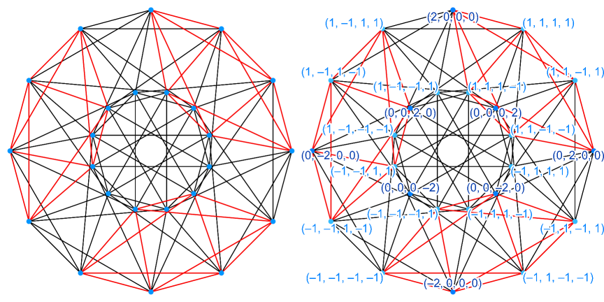
Figure 3.1: Three disjoint facets of $Y_{1}$, whose edges are marked in red, with and without coordinates. The $24$-cell layout of this diagram and others in the Appendix are based on [30, 27] and the $24$-cell visualization in the application HyperSolids [19].

for all $m\in\mathbb{N}$, where all “$\pm$” signs are independent. In this paper we reserve $m$ for the index of a sequence of polytopes or packings. A diagram of $Y_{1}$ and the coordinates of all of its vertices can be found in Figure 3.1 at the start of Section 3. Gandini and Zucco used the scaling and orientation of the $D_{4}$ lattice as generated by the vectors inside the braces of (1.4), which is a packing set of $B^{4}$ and contains all the vertices of each $Y_{m}$. The use of the $24$-cell for a high-density finite packing is a natural choice due to an appropriately scaled and oriented $24$-cell being the Dirichlet-Voronoi cell of the $D_{4}$ lattice (see [7], Chapter 21, Subsection 3.2). They calculated

$$G\left(Y_{m}\right) =4m^{4}+8m^{3}+8m^{2}+4m+1,$$ (1.5)

$$\operatorname{vol}\left(Y_{m}+B^{4}\right) =32m^{4}+64\sqrt{2}m^{3}+16\sqrt{3}\pi m^{2}+192\left(\arccos\left(\frac{1}{3}\right)-\frac{\pi}{3}\right)m+\frac{1}{2}\pi^{2};$$ (1.6)

the latter using Steiner’s formula. Then $\operatorname{vol}\left(Y_{m}+B^{4}\right)<\operatorname{vol}\left(\operatorname{conv}\left(S_{G\left(Y_{m}\right)}^{4}\right)+B^{4}\right)$ for the first time when $m=17$ and $G\left(Y_{m}\right)=375,\!769$, hence $n_{4}^{*}\leq 375,\!769$. Gandini and Zucco obtained the upper bound $n_{4}^{*}<367,\!300$ via “suitable truncations of the $24$-cell,” along with a conjectural lower bound of $n_{4}^{*}>300,\!000$ derived from the sequence $\left(Y_{m}\right)$. However, in their paper they explained neither the nature of these truncations nor the exact number of points which they obtained for the upper bound.

In this paper we prove new upper bounds for $n_{4}^{*}$ and $N_{4}^{*}$:

Theorem 1.5.

$n_{4}^{*}\leq 338,\!196$.

Theorem 1.6.

$N_{4}^{*}\leq 516,\!946$.

The remainder of this paper is organized into three main sections. In Section 2 we introduce the precise definitions and constructions for a large family of packings obtained by truncating facets of $Y_{m}$ in the same way that Wills (1985) [32] truncated edges. The result is a collection of polytopes $t_{h}^{3}\left(Y_{m}\right)$, $h\in\left\{0,\ldots,\left\lfloor\frac{m-1}{2}\right\rfloor\right\}$ (this notation is defined in Subsection 2.1) which are truncations of a single facet from the polytopes $Y_{m}$ of Gandini and Zucco’s sequence, and we obtain analogues of (1.5) and (1.6) for $t_{h}^{3}\left(Y_{m}\right)$. In Section 3, we truncate three facets from $Y_{m}$ to obtain a greater supply of polytopes $t_{\mathbf{h}}^{3}\left(Y_{m}\right)$. We then compute the number of points $G\left(t_{\mathbf{h}}^{3}\left(Y_{m}\right)\right)$ of the packing and $\operatorname{vol}\left(t_{\mathbf{h}}^{3}\left(Y_{m}\right)+B^{d}\right)$, the latter using Steiner’s formula, and prove that $n_{3}^{*}\leq 338,\!224$ via a particular packing of the form $t_{\mathbf{h}}^{3}\left(Y_{17}\right)\cap D_{4}$. At the end of this section we show that it is possible to remove $28$ points from this packing while remaining denser than the sausage, resulting in Theorem 1.5. Finally, Section 4 provides a more careful examination of the packings $t_{\mathbf{h}}^{3}\left(Y_{m}\right)$ to obtain a proof of Theorem 1.6 using the same basic ideas as Gandini and Wills (1992) [10].

2 The truncation of a single facet

First we introduce notation for the $24$ facets of the $24$-cell $Y_{m}$, $m\in\mathbb{N}$.

Definition 2.1.

Let $m\in\mathbb{N}$ and denote the facets of $Y_{m}$ by $X_{m}^{1},\ldots,X_{m}^{24}$; we number the specific facets

$$X_{m}^{1} :=m\operatorname{conv}\left\{\vphantom{\begin{pmatrix}2\\ 0\\ 0\\ 0\end{pmatrix}}\right.\! \begin{pmatrix}2\\ 0\\ 0\\ 0\end{pmatrix} \,,\, \begin{pmatrix}1\\ 1\\ 1\\ 1\end{pmatrix} \,,\, \begin{pmatrix}\hphantom{+}1\\ \hphantom{+}1\\ \hphantom{+}1\\ -1\end{pmatrix} \,,\, \begin{pmatrix}\hphantom{+}1\\ \hphantom{+}1\\ -1\\ \hphantom{+}1\end{pmatrix} \,,\, \begin{pmatrix}\hphantom{+}1\\ \hphantom{+}1\\ -1\\ -1\end{pmatrix} \,,\, \begin{pmatrix}0\\ 2\\ 0\\ 0\end{pmatrix} \!\left.\vphantom{\begin{pmatrix}2\\ 0\\ 0\\ 0\end{pmatrix}}\right\},$$ (2.1)

$$X_{m}^{2} :=m\operatorname{conv}\left\{\vphantom{\begin{pmatrix}2\\ 0\\ 0\\ 0\end{pmatrix}}\right.\! \begin{pmatrix}\hphantom{+}1\\ \hphantom{+}1\\ -1\\ \hphantom{+}1\end{pmatrix} \,,\, \begin{pmatrix}1\\ 1\\ 1\\ 1\end{pmatrix} \,,\, \begin{pmatrix}2\\ 0\\ 0\\ 0\end{pmatrix} \,,\, \begin{pmatrix}\hphantom{+}1\\ -1\\ -1\\ \hphantom{+}1\end{pmatrix} \,,\, \begin{pmatrix}0\\ 0\\ 0\\ 2\end{pmatrix} \,,\, \begin{pmatrix}\hphantom{+}1\\ -1\\ \hphantom{+}1\\ \hphantom{+}1\end{pmatrix} \!\left.\vphantom{\begin{pmatrix}2\\ 0\\ 0\\ 0\end{pmatrix}}\right\},$$ (2.2)

$$X_{m}^{3} :=m\operatorname{conv}\left\{\vphantom{\begin{pmatrix}2\\ 0\\ 0\\ 0\end{pmatrix}}\right.\! \begin{pmatrix}\hphantom{+}1\\ -1\\ \hphantom{+}1\\ -1\end{pmatrix} \,,\, \begin{pmatrix}0\\ 0\\ 2\\ 0\end{pmatrix} \,,\, \begin{pmatrix}\hphantom{+}1\\ -1\\ \hphantom{+}1\\ \hphantom{+}1\end{pmatrix} \,,\, \begin{pmatrix}2\\ 0\\ 0\\ 0\end{pmatrix} \,,\, \begin{pmatrix}\hphantom{+}1\\ \hphantom{+}1\\ \hphantom{+}1\\ -1\end{pmatrix} \,,\, \begin{pmatrix}1\\ 1\\ 1\\ 1\end{pmatrix} \!\left.\vphantom{\begin{pmatrix}2\\ 0\\ 0\\ 0\end{pmatrix}}\right\},$$ (2.3)

$$X_{m}^{10} :=m\operatorname{conv}\left\{\vphantom{\begin{pmatrix}2\\ 0\\ 0\\ 0\end{pmatrix}}\right.\! \begin{pmatrix}\hphantom{+}0\\ -2\\ \hphantom{+}0\\ \hphantom{+}0\end{pmatrix} \,,\, \begin{pmatrix}\hphantom{+}1\\ -1\\ \hphantom{+}1\\ -1\end{pmatrix} \,,\, \begin{pmatrix}\hphantom{+}1\\ -1\\ -1\\ -1\end{pmatrix} \,,\, \begin{pmatrix}\hphantom{+}1\\ -1\\ -1\\ \hphantom{+}1\end{pmatrix} \,,\, \begin{pmatrix}\hphantom{+}1\\ -1\\ \hphantom{+}1\\ \hphantom{+}1\end{pmatrix} \,,\, \begin{pmatrix}2\\ 0\\ 0\\ 0\end{pmatrix} \!\left.\vphantom{\begin{pmatrix}2\\ 0\\ 0\\ 0\end{pmatrix}}\right\},$$ (2.4)

$$X_{m}^{16} :=m\operatorname{conv}\left\{\vphantom{\begin{pmatrix}2\\ 0\\ 0\\ 0\end{pmatrix}}\right.\! \begin{pmatrix}-2\\ \hphantom{+}0\\ \hphantom{+}0\\ \hphantom{+}0\end{pmatrix} \,,\, \begin{pmatrix}-1\\ \hphantom{+}1\\ -1\\ \hphantom{+}1\end{pmatrix} \,,\, \begin{pmatrix}-1\\ \hphantom{+}1\\ -1\\ -1\end{pmatrix} \,,\, \begin{pmatrix}-1\\ -1\\ -1\\ \hphantom{+}1\end{pmatrix} \,,\, \begin{pmatrix}-1\\ -1\\ -1\\ -1\end{pmatrix} \,,\, \begin{pmatrix}\hphantom{+}0\\ \hphantom{+}0\\ -2\\ \hphantom{+}0\end{pmatrix} \!\left.\vphantom{\begin{pmatrix}2\\ 0\\ 0\\ 0\end{pmatrix}}\right\},$$ (2.5)

$$X_{m}^{17} :=m\operatorname{conv}\left\{\vphantom{\begin{pmatrix}2\\ 0\\ 0\\ 0\end{pmatrix}}\right.\! \begin{pmatrix}\hphantom{+}0\\ \hphantom{+}0\\ \hphantom{+}2\\ \hphantom{+}0\end{pmatrix} \,,\, \begin{pmatrix}\hphantom{+}1\\ -1\\ \hphantom{+}1\\ \hphantom{+}1\end{pmatrix} \,,\, \begin{pmatrix}\hphantom{+}1\\ -1\\ \hphantom{+}1\\ -1\end{pmatrix} \,,\, \begin{pmatrix}-1\\ -1\\ \hphantom{+}1\\ -1\end{pmatrix} \,,\, \begin{pmatrix}-1\\ -1\\ \hphantom{+}1\\ \hphantom{+}1\end{pmatrix} \,,\, \begin{pmatrix}\hphantom{+}0\\ -2\\ \hphantom{+}0\\ \hphantom{+}0\end{pmatrix} \!\left.\vphantom{\begin{pmatrix}2\\ 0\\ 0\\ 0\end{pmatrix}}\right\},$$ (2.6)

and also in Definition 2.7; the remaining facets may be numbered arbitrarily. For each $i\in\left\{1,\ldots,24\right\}$, let $\mathbf{u}^{i}$ be the unit outward normal to $X_{m}^{i}$, and for $\lambda\geq 0$ let $H_{i}\left(\lambda\right):=H\left(\mathbf{u}^{i},\sqrt{2}\lambda\right)$ and $H_{i}^{-}\left(\lambda\right):=H^{-}\left(\mathbf{u}^{i},\sqrt{2}\lambda\right)$.

Note that $H_{i}\left(m\right)$ is a supporting hyperplane of $Y_{m}$ and $Y_{m}=\bigcap_{i=1}^{24}H_{i}^{-}\left(m\right)$. For any $i\in\left\{1,\ldots,24\right\}$, $\mathbf{u}^{i}$ is $\frac{1}{m\sqrt{2}}$ times the centroid of $X_{m}^{i}$ (see [8], page 292, Table I (ii)), $X_{m}^{i}\subset H_{i}\left(m\right)$, and $X_{m}=\bigcap_{i=1}^{24}H_{i}^{-}\left(\lambda\right)$. For the rest of this section we will assume that $m\in\mathbb{N}$ and $h\in\left\{0,\ldots,m\right\}$ unless otherwise indicated. The following definition makes precise our usage of facet truncation when it comes to the $24$-cell. Initially we truncate a single facet of $Y_{m}$. Due to the symmetry of the $24$-cell, the specific choice of facet is irrelevant, so we may choose the regular octahedron $X_{m}^{1}$ of edge length $2m$. Color-coded physical models of various sections of the $24$-cell can be viewed at [21].

Definition 2.2.

Let $m\in\mathbb{N}$. Define the polytope obtained from the single-facet truncation of $Y_{m}$ by $t_{h}^{3}\left(Y_{m}\right):=Y_{m}\cap H_{1}^{-}\left(m-h\right)$ and denote its facets $X_{m,h}^{1},\ldots,X_{m,h}^{24}$ by

$$X_{m,h}^{i}:=\begin{cases}Y_{m}\cap H_{1}\left(m-h\right)&i=1\\ X_{m}^{i}\cap H_{i}^{-}\left(m-h\right)&i\in\left\{2,\ldots,24\right\}\end{cases}.$$

Since $\operatorname{dist}\left(\mathbf{0},X_{m}^{1}\right)=\sqrt{2}m$ (cf. the hyperplanes mentioned in [11]), the truncation $t_{h}^{3}$ removes a $\sqrt{2}h$-thick “slice” containing the facet $X_{m}^{1}$ of $Y_{m}$. The polytope $t_{h}^{3}\left(Y_{m}\right)$ is a truncation of a single facet $X_{m}^{1}$ of $Y_{m}$, where $h$ controls the “amount” of truncation, and for all $i\in\left\{1,2,\ldots,24\right\}$, the facet $X_{m,h}^{i}\subset t_{h}^{3}\left(Y_{m}\right)$ is parallel to the corresponding facet $X_{m}^{i}\subset Y_{m}$. The packing density of $t_{h}^{3}\left(Y_{m}\right)\cap D_{4}$ is (see (1.2))

$$\delta\left(t_{h}^{3}\left(Y_{m}\right)\cap D_{4}\right)=\frac{G\left(t_{h}^{3}\left(Y_{m}\right)\right)}{\operatorname{vol}\left(\operatorname{conv}\left(t_{h}^{3}\left(Y_{m}\right)\cap D_{4}\right)+B^{4}\right)}.$$

Tedious but elementary calculations (see the Appendix—Subsection LABEL:subsec:_The_vertices_of_t_=00007Bh=00007D^=00007B3=00007D(Y_m)_are_at_points_of_D_4) show that the vertices of $t_{h}^{3}\left(Y_{m}\right)$ are located at points of $D_{4}$ for all $m\in\mathbb{N}$ and $h\in\left\{0,\ldots,m\right\}$, which implies that $\operatorname{conv}\left(t_{h}^{3}\left(Y_{m}\right)\cap D_{4}\right)=t_{h}^{3}\left(Y_{m}\right)$ for all $m\in\mathbb{N}$ and $h\in\left\{0,\ldots,m\right\}$, therefore

$$\delta\left(t_{h}^{3}\left(Y_{m}\right)\cap D_{4}\right)=\frac{G\left(t_{h}^{3}\left(Y_{m}\right)\right)}{\operatorname{vol}\left(t_{h}^{3}\left(Y_{m}\right)+B^{4}\right)}.$$

In Subsections 2.2 and 2.1 we obtain formulas for $G\left(t_{h}^{3}\left(Y_{m}\right)\right)$ and $\operatorname{vol}\left(t_{h}^{3}\left(Y_{m}\right)+B^{4}\right)$ respectively in terms of only $m$ and $h$; the latter using Steiner’s formula.

2.1 The Steiner polynomial for the single-facet truncation

In this section we state the basic properties of $t_{h}^{3}$ that are necessary to compute the exact values of $G\left(t_{h}^{3}\left(Y_{m}\right)\right)$ and $\operatorname{vol}\left(t_{h}^{3}\left(Y_{m}\right)+B^{4}\right)$.

Lemma 2.3.

Let $m\in\mathbb{N}$ and $h\in\left\{0,\ldots,m\right\}$. Then

$$G\left(t_{\mathbf{h}}^{3}\left(Y_{m}\right)\right)=4m^{4}+\left(8-\frac{2h}{3}\right)m^{3}+\left(8-\left(h^{2}+h\right)\right)m^{2}\\ \,+\left(4-\frac{2h^{3}+3h^{2}+2h}{3}\right)m+\left(1-\frac{-2h^{4}+2h^{3}+5h^{2}+h}{6}\right)$$ (2.7)

Proof.

See Subsection 2.2. ∎

For the volume calculation, we know from Steiner’s formula that

$$\operatorname{vol}\left(t_{h}^{3}\left(Y_{m}\right)+B^{4}\right)=\operatorname{vol}\left(t_{h}^{3}\left(Y_{m}\right)\right)+c\left(t_{h}^{3}\left(Y_{m}\right)\right)+f\left(t_{h}^{3}\left(Y_{m}\right)\right)+e\left(t_{h}^{3}\left(Y_{m}\right)\right)+\frac{1}{2}\pi^{2},$$ (2.8)

where $\operatorname{vol}\left(t_{h}^{3}\left(Y_{m}\right)\right)$, $c\left(t_{h}^{3}\left(Y_{m}\right)\right)$, $f\left(t_{h}^{3}\left(Y_{m}\right)\right)$, and $e\left(t_{h}^{3}\left(Y_{m}\right)\right)$ are the $4$-, $3$-, $2$-, and $1$-dimensional volume components of (1.3) respectively.

Lemma 2.4.

Let $m\in\mathbb{N}$ and $h\in\left\{0,\ldots,m\right\}$, then

$$\operatorname{vol}\left(t_{h}^{3}\left(Y_{m}\right)\right) =\operatorname{vol}\left(Y_{m}\right)-\frac{4}{3}\left(\left(m+h\right)^{4}-m^{4}-3h^{4}\right),$$ (2.9)

$$c\left(t_{h}^{3}\left(Y_{m}\right)\right) =\frac{8\sqrt{2}}{3}\left(25m^{3}-\left(m+h\right)^{3}\right),$$ (2.10)

$$f\left(t_{h}^{3}\left(Y_{m}\right)\right) =\frac{2\sqrt{3}\pi}{3}\left(24m^{2}-2mh+\left(3\sqrt{3}-7\right)h^{2}\right),$$ (2.11)

$$e\left(t_{h}^{3}\left(Y_{m}\right)\right) =\left(64m-24h\right)\left(3\arccos\left(\frac{1}{3}\right)-\pi\right)+64h\arctan\left(3-2\sqrt{2}\right).$$ (2.12)

Proof.

See Subsubsections 2.3.1, 2.3.2, 2.3.3, and 2.3.4 respectively. ∎

Lemma 2.5.

Let $m\in\mathbb{N}$ and $h\in\left\{0,\ldots,m\right\}$, then

$$\operatorname{vol}\left(t_{h}^{3}\left(Y_{m}\right)+B^{4}\right) = 32m^{4}+\left[64\sqrt{2}-\frac{16}{3}h\right]m^{3}+\left[16\sqrt{3}\pi-8\sqrt{2}h-8h^{2}\right]m^{2}$$ (2.13)

$$\,+\left[64\left(3\arccos\left(\frac{1}{3}\right)-\pi\right)-\frac{4\sqrt{3}\pi}{3}h-8\sqrt{2}h^{2}-\frac{16}{3}h^{3}\right]m$$

$$\,+\,\frac{1}{2}\pi^{2}+\left[\left(64\arctan\left(3-2\sqrt{2}\right)-24\left(3\arccos\left(\frac{1}{3}\right)-\pi\right)\right)h\vphantom{\frac{\left(18-14\sqrt{3}\right)\pi}{3}}\right.$$

$$\left.\hphantom{\,+\,\frac{1}{2}\pi^{2}}\qquad+\frac{\left(18-14\sqrt{3}\right)\pi}{3}h^{2}-\frac{8\sqrt{2}}{3}h^{3}+\frac{8}{3}h^{4}\right].$$

Proof.

This result follows from (2.8) and Lemma 2.4. ∎

2.2 The number of points in $t_{h}^{3}\left(Y_{m}\right)$

We will obtain the quantity $G\left(Y_{m}\right)-G\left(t_{h}^{3}\left(Y_{m}\right)\right)$ by counting the points of $D_{4}$ in each truncated octahedron $X_{m,k}^{1}$ for $k\in\left\{0,\ldots,h-1\right\}$ and summing them up.

Proposition 2.6.

Let $m\in\mathbb{N}$ and $h\in\left\{0,\ldots,m\right\}$. Then

$$G\left(Y_{m}\right)-G\left(t_{h}^{3}\left(Y_{m}\right)\right)=\sum_{k=0}^{h-1}G\left(X_{m,k}^{1}\right).$$ (2.14)

Proof.

This method of adding up the $h$ distinct layers $X_{m,k}^{1}$ neither omits nor double counts any points of $D_{4}$ in $Y_{m}\!\left\backslash t_{h}^{3}\left(Y_{m}\right)\right.$. To see this fact, note that the distance between $X_{m,k}^{1}$ and its adjacent layer $X_{m,k+1}^{1}$ is $\operatorname{dist}\left(X_{m,k}^{1},X_{m,k+1}^{1}\right)=\sqrt{2}$ for any $k\in\left\{0,\ldots,h-1\right\}$, which is equal to the distance between adjacent hyperplanes containing translates of $D_{3}$ in $D_{4}$. These quantities are equal, so the sets $X_{m,k}^{1}$, $k\in\left\{0,\ldots,h-1\right\}$, coincide with individual layers of $D_{4}$, from which (2.14) follows. ∎

In Section 3 it will be convenient to express $G\left(Y_{m}\right)-G\left(t_{h}^{3}\left(Y_{m}\right)\right)$ as a polynomial in $m$ whose coefficients are themselves polynomials in $h$. Let $\widehat{X}_{m,h}^{1}$ be the regular octahedron whose faces have the same centroids as the faces of $X_{m,h}^{1}$, in other words, $X_{m,h}^{1}$ is obtained from $\widehat{X}_{m,h}^{1}$ via vertex truncations that remove six square pyramids of appropriate height from $\widehat{X}_{m,h}^{1}$. Basic calculations along with the linearity of the edge length of $\widehat{X}_{m,h}^{1}$ in the variable $h$ show that $\widehat{X}_{m,h}^{1}$ has edge length $2\left(m+h\right)$.

Proof of (2.7) in Lemma 2.3.

Let $k\in\left\{0,\ldots,h-1\right\}$. The intersection $\widehat{X}_{m,k}^{1}\cap D_{3}$ consists of a middle layer with $\left(\left(m+k\right)+1\right)^{2}$ points and for each $i\in\left\{1,\ldots,m+k\right\}$, two layers with $i^{2}$ points, one above the middle layer and one below, so

$$G\left(\widehat{X}_{m,k}^{1}\right)=\left(m+k+1\right)^{2}+2\sum_{i=1}^{m+k}i^{2}=\frac{2\left(m+k\right)^{3}+6\left(m+k\right)^{2}+7\left(m+k\right)+3}{3}.$$ (2.15)

Due to the vertex truncations, $G\left(X_{m,k}^{1}\right)=G\left(\widehat{X}_{m,k}^{1}\right)-6\sum_{i=1}^{k}i^{2}$, so from this equation, (2.14), and (2.15) we conclude that

$$G\left(Y_{m}\right)-G\left(t_{h}^{3}\left(Y_{m}\right)\right)=\sum_{k=0}^{h-1}\left(\frac{2\left(m+k\right)^{3}+6\left(m+k\right)^{2}+7\left(m+k\right)+3}{3}-6\sum_{i=1}^{k}i^{2}\right)\\ =\frac{2h}{3}m^{3}+\left(h^{2}+h\right)m^{2}+\frac{2h^{3}+3h^{2}+2h}{3}m+\frac{-2h^{4}+2h^{3}+5h^{2}+h}{6}.$$

∎

2.3 The vertices, edges, faces, and facets of $t_{h}^{3}\left(Y_{m}\right)$

In this subsection we prove the four equations (2.9), (2.10), (2.11), and (2.12) of Lemma 2.4. For each $i\in\left\{1,2,3\right\}$, we classify all the $i$-faces of $t_{h}^{3}\left(Y_{m}\right)$ into different types based on their interactions with the half-space $H_{1}^{-}\left(m-h\right)$, then find the $i$-volume and $\left(4-i\right)$-dimensional external angle of each $i$-face. Due to the symmetries of $Y_{m}$ and $t_{h}^{3}\left(Y_{m}\right)$, all faces within a given type have the same volume and external angle, so it is not necessary to explicitly write down all of these faces. Instead, for each type we will provide a description of a single “representative face” with which the calculations will be done. Diagrams of these faces are shown in the Appendix, Figures LABEL:fig:_Truncated_facets_of_t_=00007Bh=00007D^=00007B3=00007D(Y_m) and LABEL:fig:_Truncated_faces_and_edges_of_t_=00007Bh=00007D^=00007B3=00007D(Y_m).

2.3.1 The $4$-volume of $Y_{m}\!\left\backslash t_{h}^{3}\left(Y_{m}\right)\right.$

Let $\widehat{Y}_{m,h}:=Y_{m}\!\left\backslash t_{h}^{3}\left(Y_{m}\right)\right.$. In this subsubsection we compute the four-dimensional volume $\operatorname{vol}\left(\widehat{Y}_{m,h}\right)$, then we can obtain $\operatorname{vol}\left(t_{h}^{3}\left(Y_{m}\right)\right)=\operatorname{vol}\left(Y_{m}\right)-\operatorname{vol}\left(\widehat{Y}_{m,-h}\right)$.

Proof of (2.10) in Lemma 2.4.

We calculate the ($4$-dimensional) volume of $\widehat{Y}_{m,h}$ by finding the $3$-dimensional volume of each cross-section $Y_{m}\cap H_{1}\left(\lambda\right)\subset\widehat{Y}_{m,h}$ and computing the integral

$$\operatorname{vol}\left(\widehat{Y}_{m,h}\right)=\sqrt{2}\int_{m-h}^{m}\operatorname{vol}_{3}\left(Y_{m}\cap H_{1}\left(\lambda\right)\right)\,d\lambda.$$ (2.16)

(The factor of $\sqrt{2}$ occurs because $\operatorname{dist}\left(\mathbf{0},H_{m}\left(\lambda\right)\right)=\sqrt{2}\lambda$.) We wish to find the integrand $\operatorname{vol}_{3}\left(Y_{m}\cap H_{1}\left(\lambda\right)\right)$. The intersection $Y_{m}\cap H_{1}\left(\lambda\right)$ is a truncated octahedron for all $\lambda\in\left(0,m\right)$ and is contained inside $\widehat{X}_{m,h}^{1}$, which has edge length $2\left(m+h\right)=2\left(2m-\lambda\right)$. Its volume can be found by subtracting the volume of six square pyramids with edge lengths $2\left(m-\lambda\right)$ from $\operatorname{vol}_{3}\left(\widehat{X}_{m,h}^{1}\right)$, so

$$\operatorname{vol}_{3}\left(Y_{m}\cap H_{1}\left(\lambda\right)\right)=\frac{8\sqrt{2}}{3}\left(\left(m+h\right)^{3}-3h^{3}\right).$$ (2.17)

Using this expression, evaluating the integral (2.16) gives

$$\operatorname{vol}\left(\widehat{Y}_{m,h}\right)=\sqrt{2}\int_{m-h}^{m}\operatorname{vol}_{3}\left(Y_{m}\cap H_{m}\left(\lambda\right)\right)\,d\lambda=\frac{4}{3}\left(\left(m+h\right)^{4}-m^{4}-3h^{4}\right),$$

from which (2.9) follows. ∎

2.3.2 The $3$-dimensional facets

We wish to find the three-dimensional volume $\operatorname{vol}_{3}\left(t_{h}^{3}\left(Y_{m}\right)\right)$ obtained from the facets of $t_{h}^{3}\left(Y_{m}\right)$, and to do so we investigate the facets of $t_{h}^{3}\left(Y_{m}\right)$.

Definition 2.7.

Order the facets $X_{m}^{1},\ldots,X_{m}^{24}$ of $Y_{m}$ such that $X_{m}^{2},\ldots,X_{m}^{9}$ share a face with $X_{m}^{1}$ and $X_{m}^{10},\ldots,X_{m}^{15}$ share a vertex with but not a face of $X_{m}^{1}$. For $h\in\left\{0,\ldots,m\right\}$, define $t_{h}^{2}$ and $t_{h}^{0}$ on these facets by $t_{h}^{2}\left(X_{m}^{i}\right):=X_{m}^{i}\cap H_{1}^{-}\left(m-h\right)$ for $i\in\left\{2,\ldots,9\right\}$ and $t_{h}^{0}\left(X_{m}^{k}\right):=X_{m}^{k}\cap H_{1}^{-}\left(m-h\right)$ for $k\in\left\{10,\ldots,15\right\}$.

Note that $X_{m}^{2}$, $X_{m}^{3}$, and $X_{m}^{10}$ were already defined in Definition 2.1, but we can choose an ordering of the facets so that these two definitions are consistent. As this notation implies, the adjacent facets $t_{h}^{2}\left(X_{m}^{i}\right)$ and $t_{h}^{0}\left(X_{m}^{k}\right)$ of $Y_{m}$ are obtained by truncating one face and one vertex of the octahedron respectively. When $m\in\mathbb{N}$ and $0<h<m$ the facets $X_{m}^{1},\ldots,X_{m}^{24}$ of $Y_{m}$, and the corresponding facets $X_{m,h}^{i}$ of $t_{h}^{3}\left(Y_{m}\right)$, can be categorized into four types based on their intersection with the half-space $H_{1}^{-}\left(m-h\right)$.

1. The intersection $X_{m}^{1}\cap H_{1}^{-}\left(m-h\right)$ is the empty set, so $X_{m}^{1}\subset Y_{m}$ corresponds to a single new facet $X_{m,h}^{1}\subset t_{h}^{3}\left(Y_{m}\right)$ that is parallel to $X_{m}^{1}$. Since $X_{m,h}^{1}$ is a cross-section parallel to a facet of $Y_{m}$, it is a truncated octahedron (see [4, 22, 21]) with six square faces of edge length $2h$ and eight hexagonal faces with edge lengths alternating between $2h$ and $2\left(m-h\right)$.

2. Eight facets of $Y_{m}$, which after reordering we refer to as $X_{m}^{2},\ldots,X_{m}^{9}$, are truncated at the face where the facet intersects $H_{1}\left(m-h\right)$. The original facet $X_{m}^{i}$ shares three of its six vertices with its corresponding face-truncated facet $X_{m}^{i}\cap H_{1}^{-}\left(m-h\right)\subset t_{h}^{3}\left(Y_{m}\right)$. Hence the facets $t_{h}^{2}\left(X_{m}^{2}\right),\ldots,t_{h}^{2}\left(X_{m}^{9}\right)$ of $t_{h}^{3}\left(Y_{m}\right)$ are face-truncations of the octahedron and are rigid motions of the representative facet

   $$t_{h}^{2}\left(X_{m}^{\hexagon}\right) = \operatorname{conv}\left\{\begin{pmatrix}2m-h\\ -h\\ \hphantom{+}h\\ \hphantom{+}h\end{pmatrix},\begin{pmatrix}2m-h\\ -h\\ \hphantom{+}h\\ -h\end{pmatrix},\begin{pmatrix}\hphantom{+}m\\ m-2h\\ \hphantom{+}m\\ -m\end{pmatrix},\begin{pmatrix}\hphantom{+}m-h\\ \hphantom{+}m-h\\ \hphantom{+}m+h\\ -m+h\end{pmatrix},\right.$$

   $$\hphantom{\operatorname{conv}\left\{\vphantom{\begin{pmatrix}2m-h\\ -h\\ \hphantom{+}h\\ \hphantom{+}h\end{pmatrix}}\right.}\!\!\left.\begin{pmatrix}m-h\\ m-h\\ m+h\\ m-h\end{pmatrix},\begin{pmatrix}m\\ m-2h\\ m\\ m\end{pmatrix},\begin{pmatrix}\hphantom{+}m\\ -m\\ \hphantom{+}m\\ \hphantom{+}m\end{pmatrix},\begin{pmatrix}0\\ 0\\ 2m\\ 0\end{pmatrix},\begin{pmatrix}\hphantom{+}m\\ -m\\ \hphantom{+}m\\ -m\end{pmatrix}\right\},$$

   where

   $$X_{m}^{\hexagon}:=\operatorname{conv}\left\{\begin{pmatrix}2m\\ 0\\ 0\\ 0\end{pmatrix},\begin{pmatrix}m\\ m\\ m\\ m\end{pmatrix},\begin{pmatrix}\hphantom{+}m\\ \hphantom{+}m\\ \hphantom{+}m\\ -m\end{pmatrix},\begin{pmatrix}\hphantom{+}m\\ -m\\ \hphantom{+}m\\ \hphantom{+}m\end{pmatrix},\begin{pmatrix}0\\ 0\\ 2m\\ 0\end{pmatrix},\begin{pmatrix}\hphantom{+}m\\ -m\\ \hphantom{+}m\\ -m\end{pmatrix}\right\}.$$

3. Six facets of $Y_{m}$, which after reordering we refer to as $X_{m}^{10},\ldots,X_{m}^{15}$, are truncated at the vertex where the facet intersects $H_{1}\left(m-h\right)$. The original facet $X_{m}^{k}$ shares five of its six vertices with its corresponding vertex-truncated facet $X_{m}^{k}\cap H_{1}^{-}\left(m-h\right)\subset t_{h}^{3}\left(Y_{m}\right)$. So the facets $t_{h}^{0}\left(X_{m}^{10}\right),\ldots,t_{h}^{0}\left(X_{m}^{15}\right)$ of $t_{h}^{3}\left(Y_{m}\right)$ are vertex-truncations of the octahedron and are rigid motions of the representative facet

   $$t_{h}^{0}\left(X_{m}^{\square}\right) = \operatorname{conv}\left\{\begin{pmatrix}2m-h\\ -h\\ \hphantom{+}h\\ \hphantom{+}h\end{pmatrix},\begin{pmatrix}2m-h\\ -h\\ \hphantom{+}h\\ -h\end{pmatrix},\begin{pmatrix}2m-h\\ -h\\ -h\\ -h\end{pmatrix},\begin{pmatrix}2m-h\\ -h\\ -h\\ \hphantom{+}h\end{pmatrix},\right.$$

   $$\hphantom{\operatorname{conv}\left\{\vphantom{\begin{pmatrix}2m-h\\ -h\\ \hphantom{+}h\\ \hphantom{+}h\end{pmatrix}}\right.}\!\!\left.\begin{pmatrix}\hphantom{+}1\\ -1\\ \hphantom{+}1\\ \hphantom{+}1\end{pmatrix},\begin{pmatrix}\hphantom{+}1\\ -1\\ \hphantom{+}1\\ -1\end{pmatrix},\begin{pmatrix}\hphantom{+}1\\ -1\\ -1\\ -1\end{pmatrix},\begin{pmatrix}\hphantom{+}1\\ -1\\ -1\\ \hphantom{+}1\end{pmatrix},\begin{pmatrix}\hphantom{+}0\\ -2\\ \hphantom{+}0\\ \hphantom{+}0\end{pmatrix}\right\},$$

   where

   $$X_{m}^{\square}:=\operatorname{conv}\left\{\begin{pmatrix}2\\ 0\\ 0\\ 0\end{pmatrix},\begin{pmatrix}\hphantom{+}1\\ -1\\ \hphantom{+}1\\ \hphantom{+}1\end{pmatrix},\begin{pmatrix}\hphantom{+}1\\ -1\\ \hphantom{+}1\\ -1\end{pmatrix},\begin{pmatrix}\hphantom{+}1\\ -1\\ -1\\ -1\end{pmatrix},\begin{pmatrix}\hphantom{+}1\\ -1\\ -1\\ \hphantom{+}1\end{pmatrix},\begin{pmatrix}\hphantom{+}0\\ -2\\ \hphantom{+}0\\ \hphantom{+}0\end{pmatrix}\right\}.$$

4. The remaining nine facets $X_{m}^{16},\ldots,X_{m}^{24}\subset Y_{m}$ are unmodified by the facet truncation because they lie entirely in the closed half-space $H_{1}^{-}\left(m-h\right)$, hence $X_{m}^{l}=X_{m}^{l}\cap H_{1}^{-}\left(m-h\right)\subset t_{h}^{3}\left(Y_{m}\right)$.

To show (2.10) we establish the following statements. The external angle $\theta\left(Y_{m},F\right)$ of any facet $F$ is $\frac{1}{2}$, so we do not need to perform external angle computations for these facets.

Lemma 2.8.

Let $m\in\mathbb{N}$ and $h\in\left\{0,\ldots,m\right\}$. The four kinds of representative facets of $t_{h}^{3}\left(Y_{m}\right)$ described above have the following $3$-volumes:

$$\operatorname{vol}_{3}\left(X_{m,h}^{1}\right) =\frac{8\sqrt{2}}{3}\left(\left(m+h\right)^{3}-3h^{3}\right),$$ (2.18)

$$\operatorname{vol}_{3}\left(t_{h}^{2}\left(X_{m}^{i}\right)\right) =\frac{2\sqrt{2}}{3}\left(5m^{3}+3h^{3}-\left(m+h\right)^{3}\right),$$ (2.19)

$$\operatorname{vol}_{3}\left(t_{h}^{0}\left(X_{m}^{k}\right)\right) =\frac{4\sqrt{2}}{3}\left(2m^{3}-h^{3}\right),$$ (2.20)

$$\operatorname{vol}_{3}\left(X_{m}^{l}\right) =\frac{8\sqrt{2}}{3}m^{3},$$ (2.21)

where $i\in\left\{2,\ldots,9\right\}$, $k\in\left\{10,\ldots,15\right\}$, and $l\in\left\{16,\ldots,24\right\}$.

Proof.

Equation (2.21) follows directly from the formula for the volume of a regular octahedron and (2.18) was already obtained as (2.17) in the previous subsubsection. The cross-section of $X_{m}^{i}$ parallel to $H^{i}\left(\lambda\right)$ is $X_{m}^{i}\cap H^{i}\left(\lambda\right)$, a large equilateral triangle of edge length $2\left(2m-\lambda\right)$ with its vertices truncated via removing an equilateral triangle of edge length $2\left(m-\lambda\right)$ from each vertex. So $\operatorname{area}\left(X_{m}^{i}\cap H^{i}\left(\lambda\right)\right)=\sqrt{3}\left(2m-\lambda\right)^{2}-3\sqrt{3}\left(m-\lambda\right)^{2}$ and

$$\operatorname{vol}_{3}\left(t_{h}^{2}\left(X_{m}^{i}\right)\right) = \frac{2\sqrt{6}}{3}\int_{0}^{m-h}\operatorname{area}\left(X_{m}^{i}\cap H^{i}\left(\lambda\right)\right)\,d\lambda$$

$$= \frac{2\sqrt{2}}{3}\left(5m^{3}+3h^{3}-\left(m+h\right)^{3}\right),$$

showing (2.19). (The distance between two opposite faces of $X_{m}^{i}$ is $\frac{2\sqrt{6}}{3}m$.) For (2.20), let $\mathbf{v}_{0}=X_{m}^{i}\cap Y_{m}$, $\mathbf{v}$ be any of the four neighboring vertices of $X_{m}^{i}$, and let $E=\operatorname{conv}\left\{\mathbf{v}_{0},\mathbf{v}\right\}$ be the edge of $Y_{m}$ containing these vertices. The hyperplane $H^{1}\left(m-h\right)$ intersects $E$ at $\frac{h}{m}$ of the distance from $\mathbf{v}_{0}$ to $\mathbf{v}$. Since $E$ has length $2m$, $X_{m}^{i}\!\left\backslash\left(t_{h}^{0}\left(X_{m}^{i}\right)\right)\right.$ is a square pyramid of edge length $2h$. So

$$\operatorname{vol}_{3}\left(t_{h}^{0}\left(X_{m}^{i}\right)\right) = \operatorname{vol}_{3}\left(X_{m}^{i}\right)-\operatorname{vol}_{3}\left(X_{m}^{i}\left\backslash\,t_{h}^{0}\left(X_{m}^{i}\right)\right.\right)$$

$$= \frac{4\sqrt{2}}{3}\left(2m^{3}-h^{3}\right).$$

∎

Proof of (2.10) in Lemma 2.4.

The discussion at the beginning of this subsubsection, along with Lemma 2.8, imply that

$$c\left(t_{h}^{3}\left(Y_{m}\right)\right) = \sum_{i=1}^{24}\operatorname{vol}_{3}\left(X_{m,h}^{i}\right)$$

$$= 1\cdot\operatorname{vol}_{3}\left(X_{m,h}^{1}\right)+8\cdot\operatorname{vol}_{3}\left(t_{h}^{2}\left(X_{m}^{i}\right)\right)+6\cdot\operatorname{vol}_{3}\left(t_{h}^{0}\left(X_{m}^{k}\right)\right)+9\cdot\operatorname{vol}_{3}\left(X_{m}^{l}\right)$$

$$= \frac{8\sqrt{2}}{3}\left(25m^{3}-\left(m+h\right)^{3}\right).$$

∎

2.3.3 The $2$-dimensional faces

Denote the $96$ triangular faces of $Y_{m}$ by $T_{m}^{1},\ldots,T_{m}^{96}$. The $102$ faces of $t_{h}^{3}\left(Y_{m}\right)$ can also be categorized into five types based on their relationship to $H_{1}^{-}\left(m-h\right)$.

Definition 2.9.

Let $T_{m}^{i}$ and $T_{m}^{j}$ be faces of $Y_{m}$ such that $T_{m}^{j}\cap X_{m}^{1}$ is an edge and $T_{m}^{k}\cap X_{m}^{1}$ is a vertex. Then define $t_{h}^{1}\left(T_{m}^{j}\right):=T_{m}^{j}\cap H_{i}^{-}\left(m-h\right)$ and $t_{h}^{0}\left(T_{m}^{k}\right):=T_{m}^{k}\cap H_{i}^{-}\left(m-h\right)$.

$t_{h}^{1}\left(T_{m}^{i}\right)$ is an edge truncation of the triangular face $T_{m}^{i}$, hence is just a smaller triangle with the same shape. In contrast, $t_{h}^{0}\left(T_{m}^{j}\right)$ is a vertex truncation of $T_{m}^{j}$ and is an isosceles trapezium. As in the previous subsubsection, the faces can be reordered as follows.

1. $6$ square faces $Q_{m,h}^{1},\ldots,Q_{m,h}^{6}$ which are rigid motions of

   $$Q_{m,h}:=\operatorname{conv}\left\{\begin{pmatrix}2m-h\\ -h\\ \hphantom{+}h\\ \hphantom{+}h\end{pmatrix},\begin{pmatrix}2m-h\\ -h\\ \hphantom{+}h\\ -h\end{pmatrix},\begin{pmatrix}2m-h\\ -h\\ -h\\ -h\end{pmatrix},\begin{pmatrix}2m-h\\ -h\\ -h\\ \hphantom{+}h\end{pmatrix}\right\}.$$

   These faces are new and do not correspond to any face of $Y_{m}$.

2. $8$ hexagonal faces $H_{m,h}^{1},\ldots,H_{m,h}^{8}$ which are rigid motions of

   $$H_{m,h}:=\operatorname{conv}\left\{\begin{pmatrix}2m-h\\ -h\\ -h\\ \hphantom{+}h\end{pmatrix},\begin{pmatrix}2m-h\\ -h\\ \hphantom{+}h\\ \hphantom{+}h\end{pmatrix},\begin{pmatrix}m\\ m-2h\\ m\\ m\end{pmatrix},\begin{pmatrix}m-h\\ m-h\\ m-h\\ m+h\end{pmatrix},\begin{pmatrix}\hphantom{+}m-h\\ \hphantom{+}m-h\\ -m+h\\ \hphantom{+}m+h\end{pmatrix},\begin{pmatrix}\hphantom{+}m\\ m-2h\\ -m\\ \hphantom{+}m\end{pmatrix}\right\}.$$

3. $12$ triangular faces $t_{h}^{1}\left(T_{m}^{9}\right),\ldots,t_{h}^{1}\left(T_{m}^{20}\right)$ which are rigid motions of

   $$t_{h}^{1}\left(T_{m}^{\triangledown}\right)=\operatorname{conv}\left\{\begin{pmatrix}2m-h\\ -h\\ \hphantom{+}h\\ \hphantom{+}h\end{pmatrix},\begin{pmatrix}\hphantom{+}m\\ -m\\ \hphantom{+}m\\ \hphantom{+}m\end{pmatrix},\begin{pmatrix}m\\ m-2h\\ m\\ m\end{pmatrix}\right\},$$

   where

   $$T_{m}^{\triangledown}:=\operatorname{conv}\left\{\begin{pmatrix}2m\\ 0\\ 0\\ 0\end{pmatrix},\begin{pmatrix}\hphantom{+}m\\ -m\\ \hphantom{+}m\\ \hphantom{+}m\end{pmatrix},\begin{pmatrix}m\\ m\\ m\\ m\end{pmatrix}\right\}.$$

4. $24$ isosceles trapezium faces $t_{h}^{0}\left(T_{m}^{21}\right),\ldots,t_{h}^{0}\left(T_{m}^{44}\right)$ which are rigid motions of

   $$t_{h}^{0}\left(T_{m}^{\triangle}\right)=\operatorname{conv}\left\{\begin{pmatrix}2m-h\\ -h\\ \hphantom{+}h\\ -h\end{pmatrix},\begin{pmatrix}2m-h\\ -h\\ \hphantom{+}h\\ \hphantom{+}h\end{pmatrix},\begin{pmatrix}\hphantom{+}m\\ -m\\ \hphantom{+}m\\ \hphantom{+}m\end{pmatrix},\begin{pmatrix}\hphantom{+}m\\ -m\\ \hphantom{+}m\\ -m\end{pmatrix}\right\},$$

   where

   $$T_{m}^{\triangle}:=\operatorname{conv}\left\{\begin{pmatrix}2m\\ 0\\ 0\\ 0\end{pmatrix},\begin{pmatrix}\hphantom{+}m\\ -m\\ \hphantom{+}m\\ \hphantom{+}m\end{pmatrix},\begin{pmatrix}\hphantom{+}m\\ -m\\ \hphantom{+}m\\ -m\end{pmatrix}\right\}.$$

   Each of these faces shares a single vertex with $X_{m,h}^{1}$.

5. $52$ triangular faces $T_{m}^{45},\ldots,T_{m}^{96}$ which are unchanged from the corresponding faces in $Y_{m}$.

Lemma 2.10.

The representative faces $Q_{m,h}$, $H_{m,h}$, $t_{h}^{1}\left(T_{m}^{\triangledown}\right)$, $t_{h}^{0}\left(T_{m}^{\triangle}\right)$, and $T_{m}$ have the following areas and external angles:

$$\operatorname{area}\left(Q_{m,h}\right) =4h^{2}, \theta\left(t_{h}^{3}\left(Y_{m}\right),Q_{m,h}\right) =\frac{1}{4},$$

$$\operatorname{area}\left(H_{m,h}\right) =\sqrt{3}\left(m+h\right)^{2}-3\sqrt{3}h^{2}, \theta\left(t_{h}^{3}\left(Y_{m}\right),H_{m,h}\right) =\frac{1}{6},$$

$$\operatorname{area}\left(t_{h}^{1}\left(T_{m}^{\triangledown}\right)\right) =\sqrt{3}\left(m-h\right)^{2}, \theta\left(t_{h}^{3}\left(Y_{m}\right),t_{h}^{1}\left(T_{m}^{\triangledown}\right)\right) =\frac{1}{6},$$

$$\operatorname{area}\left(t_{h}^{0}\left(T_{m}^{\triangle}\right)\right) =\sqrt{3}m^{2}-\sqrt{3}h^{2}, \theta\left(t_{h}^{3}\left(Y_{m}\right),t_{h}^{0}\left(T_{m}^{\triangle}\right)\right) =\frac{1}{6},$$

$$\operatorname{area}\left(T_{m}\right) =\sqrt{3}m^{2}, \theta\left(t_{h}^{3}\left(Y_{m}\right),T_{m}\right) =\frac{1}{6}.$$

Proof.

The equations for the areas follow from elementary calculations. As for the external angles, the hexagonal face $H_{m,h}$ is parallel to the face $\operatorname{conv}\left\{\left(2m,0,0,0\right)^{\mathsf{T}},\left(m,m,m,m\right)^{\mathsf{T}},\left(m,m,-m,m\right)^{\mathsf{T}}\right\}$ of $Y_{m}$, which is the intersection of the two facets $X_{m}^{1}$ and $X_{m}^{2}$. Their outward unit normals $\mathbf{u}^{1}$ and $\mathbf{u}^{2}$ meet at the angle of $\arccos\left(\mathbf{u}^{1}\cdot\mathbf{u}^{2}\right)=\frac{\pi}{3}$, so $\theta\left(t_{h}^{3}\left(Y_{m}\right),H_{m,h}\right)=\frac{\arccos\left(\mathbf{u}^{1}\cdot\mathbf{u}^{2}\right)}{2\pi}=\frac{1}{6}$. Similarly, $t_{h}^{1}\left(T_{m}^{\triangledown}\right)$, $t_{h}^{0}\left(T_{m}^{\triangle}\right)$, and $T_{m}$ are also parallel to faces of $Y_{m}$, so almost identical calculations result in $\theta\left(t_{h}^{3}\left(Y_{m}\right),t_{h}^{1}\left(T_{m}^{\triangledown}\right)\right)=\theta\left(t_{h}^{3}\left(Y_{m}\right),t_{h}^{0}\left(T_{m}^{\triangle}\right)\right)=\theta\left(t_{h}^{3}\left(Y_{m}\right),T_{m}\right)=\frac{1}{6}$. Finally, the square face $Q_{m,h}$ is the intersection of $X_{m,h}^{1}$ and the vertex-truncation of $X_{m}^{10}$, which has outward unit normal $\mathbf{u}^{10}$, so $\theta\left(t_{h}^{3}\left(Y_{m}\right),Q_{m,h}\right)=\frac{\arccos\left(\mathbf{u}^{1}\cdot\mathbf{u}^{10}\right)}{2\pi}=\frac{1}{4}$. ∎

Proof of (2.11) in Lemma 2.4.

The discussion at the beginning of this subsubsection, along with Lemma 2.10, imply that

$$f\left(t_{h}^{3}\left(Y_{m}\right)\right) = \sum_{F\in\mathscr{F}_{2}\left(t_{h}^{3}\left(Y_{m}\right)\right)}\operatorname{area}\left(F\right)\theta\left(t_{h}^{3}\left(Y_{m}\right),F\right)\kappa_{2}$$

$$= 6\operatorname{area}\left(Q_{m,h}\right)\theta\left(t_{h}^{3}\left(Y_{m}\right),Q_{m,h}\right)\pi+8\operatorname{area}\left(H_{m,h}\right)\theta\left(t_{h}^{3}\left(Y_{m}\right),H_{m,h}\right)\pi$$

$$\,+\,12\operatorname{area}\left(t_{h}^{1}\left(T_{m}^{\triangledown}\right)\right)\theta\left(t_{h}^{3}\left(Y_{m}\right),t_{h}^{1}\left(T_{m}^{\triangledown}\right)\right)\pi$$

$$\,+\,24\operatorname{area}\left(t_{h}^{0}\left(T_{m}^{\triangle}\right)\right)\theta\left(t_{h}^{3}\left(Y_{m}\right),t_{h}^{0}\left(T_{m}^{\triangle}\right)\right)\pi+52\operatorname{area}\left(T_{m}\right)\theta\left(t_{h}^{3}\left(Y_{m}\right),T_{m}\right)\pi$$

$$= \frac{2\sqrt{3}\pi}{3}\left(24m^{2}-2mh+\left(3\sqrt{3}-7\right)h^{2}\right).$$

∎

2.3.4 The $1$-dimensional edges

The $24$-cell $Y_{m}$ has $96$ edges $E_{m}^{1},\ldots,E_{m}^{96}$ but the truncation shrinks some edges and adds four new edges near each vertex of the facet $X_{m,h}^{1}$, for a total of $120$ edges of $t_{h}^{3}\left(Y_{m}\right)$.

Definition 2.11.

Let $E_{m}$ be an edge of $Y_{m}$ with one vertex in $X_{m}^{1}$ and the other vertex not in $X_{m}^{1}$. Then define $t_{h}^{0}\left(E_{m}\right):=E_{m}\cap H_{1}^{-}\left(m-h\right)$.

The edges of $t_{h}^{3}\left(Y_{m}\right)$ can be sorted into four types based on their intersections with $H_{1}^{-}\left(m-h\right)$. The first two types are new edges (that do not exist in $Y_{m}$) while the other two are subsets of existing edges in $Y_{m}$.

1. $24$ new edges $E_{m,h}^{\square,1},\ldots,E_{m,h}^{\square,24}$ which are appropriate rigid motions of

   $$E_{m,h}^{\square}:=\operatorname{conv}\left\{\begin{pmatrix}2m-h\\ -h\\ \hphantom{+}h\\ \hphantom{+}h\end{pmatrix},\begin{pmatrix}2m-h\\ -h\\ \hphantom{+}h\\ -h\end{pmatrix}\right\}.$$

   Each of these edges borders a square face of $X_{m,h}^{1}$.

2. $12$ edges $E_{m,h}^{\hexagon,1},\ldots,E_{m,h}^{\hexagon,12}$ which are appropriate rigid motions of the representative edge

   $$E_{m,h}^{\hexagon}:=\operatorname{conv}\left\{\begin{pmatrix}2m-h\\ -h\\ \hphantom{+}h\\ \hphantom{+}h\end{pmatrix},\begin{pmatrix}m\\ m-2h\\ m\\ m\end{pmatrix}\right\}.$$

   Each of these edges borders two adjacent hexagonal faces of $X_{m,h}^{1}$ but not a square face.

3. $24$ edges $t_{h}^{0}\left(E_{m}^{13}\right),\ldots,t_{h}^{0}\left(E_{m}^{36}\right)$ which are appropriate rigid motions of

   $$t_{h}^{0}\left(E_{m}^{\triangle}\right)=\operatorname{conv}\left\{\begin{pmatrix}2m-h\\ -h\\ \hphantom{+}h\\ \hphantom{+}h\end{pmatrix},\begin{pmatrix}\hphantom{+}m\\ -m\\ \hphantom{+}m\\ \hphantom{+}m\end{pmatrix}\right\},\qquad\text{where}\qquad E_{m}^{\triangle}:=\operatorname{conv}\left\{\begin{pmatrix}2m\\ 0\\ 0\\ 0\end{pmatrix},\begin{pmatrix}\hphantom{+}m\\ -m\\ \hphantom{+}m\\ \hphantom{+}m\end{pmatrix}\right\}\text{.}$$

4. $60$ edges $E_{m}^{37},\ldots,E_{m}^{96}$ which are unchanged from the corresponding edges in $Y_{m}$.

It follows directly from the definition that their lengths are

$$\ell\left(E_{m}\right)=2m,\qquad\ell\left(E_{m,h}^{\square}\right)=2h,\qquad\ell\left(E_{m,h}^{\hexagon}\right)=\ell\left(t_{h}^{0}\left(E_{m}^{\triangle}\right)\right)=2\left(m-h\right)\text{.}$$ (2.22)

Each edge $E$ is the intersection of three facets so the intersection of its normal cone with $S^{2}$ is a spherical triangle, and to calculate its area we use L’Huilier’s Theorem (see [26], page 70):

Theorem 2.12 (L’Huilier’s Theorem).

Let $\operatorname{pos}\left\{\mathbf{v}^{1},\mathbf{v}^{2},\mathbf{v}^{3}\right\}\cap S^{2}$ be a spherical triangle, then

$$\tan\left(\frac{a_{1,2,3}}{4}\right)=\sqrt{\begin{array}[]{l}{\displaystyle\tan\left(\frac{a_{1,2}+a_{1,3}+a_{2,3}}{4}\right)\tan\left(\frac{-a_{1,2}+a_{1,3}+a_{2,3}}{4}\right)}\\ {\displaystyle\,\cdot\tan\left(\frac{a_{1,2}-a_{1,3}+a_{2,3}}{4}\right)\tan\left(\frac{a_{1,2}+a_{1,3}-a_{2,3}}{4}\right)}\end{array}},$$

where $a_{i,j}$ is the angle between $\mathbf{v}^{i}$ and $\mathbf{v}^{j}$ and $a_{1,2,3}$ is the spherical area of $\operatorname{pos}\left\{\mathbf{v}^{1},\mathbf{v}^{2},\mathbf{v}^{3}\right\}\cap S^{2}$.

Lemma 2.13.

The representative edges $E_{m,h}^{\hexagon}$, $E_{m,h}^{\square}$, $t_{h}^{0}\left(E_{m}^{\triangle}\right)$, and $E_{m}$ have the following external angles:

$$\theta\left(t_{h}^{3}\left(Y_{m}\right),E_{m,h}^{\hexagon}\right) =\frac{3\arccos\left(\frac{1}{3}\right)-\pi}{4\pi},$$ (2.23)

$$\theta\left(t_{h}^{3}\left(Y_{m}\right),E_{m,h}^{\square}\right) =\frac{4\arctan\left(3-2\sqrt{2}\right)}{4\pi},$$ (2.24)

$$\theta\left(t_{h}^{3}\left(Y_{m}\right),t_{h}^{0}\left(E_{m}^{\triangle}\right)\right) =\frac{3\arccos\left(\frac{1}{3}\right)-\pi}{4\pi},$$ (2.25)

$$\theta\left(t_{h}^{3}\left(Y_{m}\right),E_{m}\right) =\frac{3\arccos\left(\frac{1}{3}\right)-\pi}{4\pi}.$$ (2.26)

Proof.

The spherical triangles formed by the normal cones of $E_{m,h}^{\hexagon}$, $t_{h}^{0}\left(E_{m}^{\triangle}\right)$, and $E_{m}$ have the same angles as the spherical triangle mentioned in [11], Part (A), from which (2.23), (2.25), and (2.26) all follow. The spherical triangle formed by the normal cone of $E_{m,h}^{\square}$ has outward normals $\mathbf{u}^{1}$, $\mathbf{u}^{2}$, and $\mathbf{u}^{10}$, so $\arccos\left(\mathbf{u}^{1}\cdot\mathbf{u}^{2}\right)=\arccos\left(\mathbf{u}^{2}\cdot\mathbf{u}^{10}\right)=\frac{\pi}{3}$ and $\arccos\left(\mathbf{u}^{1}\cdot\mathbf{u}^{10}\right)=\frac{\pi}{2}$, and so L’Huilier’s Theorem gives (2.24):

$$\operatorname{area}\left(N\left(t_{h}^{3}\left(Y_{m}\right),E_{m,h}^{\square}\right)\cap S^{2}\right) = 4\arctan\sqrt{\tan\left(\frac{7\pi}{24}\right)\tan\left(\frac{3\pi}{24}\right)\tan\left(\frac{3\pi}{24}\right)\tan\left(\frac{\pi}{24}\right)}$$

$$= 4\arctan\left(3-2\sqrt{2}\right).$$

∎

Proof of (2.12) in Lemma 2.4.

The discussion at the beginning of this subsubsection, along with (2.22) and Lemma 2.13, imply that

$$e\left(t_{h}^{3}\left(Y_{m}\right)\right) = \sum_{E\in\mathscr{F}_{1}\left(t_{h}^{3}\left(Y_{m}\right)\right)}\ell\left(E\right)\theta\left(t_{h}^{3}\left(Y_{m}\right),E\right)\kappa_{3}$$

$$= 12\ell\left(E_{m,h}^{\square}\right)\theta\left(t_{h}^{3}\left(Y_{m}\right),E_{m,h}^{\square}\right)\kappa_{3}+24\ell\left(E_{m,h}^{\hexagon}\right)\theta\left(t_{h}^{3}\left(Y_{m}\right),E_{m,h}^{\square}\right)\kappa_{3}$$

$$\,+\,24\ell\left(t_{h}^{0}\left(E_{m}^{\triangle}\right)\right)\theta\left(t_{h}^{3}\left(Y_{m}\right),t_{h}^{0}\left(E_{m}^{\triangle}\right)\right)\kappa_{3}+60\ell\left(E_{m}\right)\theta\left(t_{h}^{3}\left(Y_{m}\right),E_{m}\right)\kappa_{3}$$

$$= \left(64m-24h\right)\left(3\arccos\left(\frac{1}{3}\right)-\pi\right)+16h\arctan\left(3-2\sqrt{2}\right).$$

∎

3 The truncation of three facets and the upper bound $n_{4}^{*}\leq 338,\!196$

In this section we truncate three facets of $Y_{m}$. Since the $24$-cell has three pairwise disjoint facets, in the next subsection we define the polytope $t_{\mathbf{h}}^{3}\left(Y_{m}\right)$ obtained from truncating three such facets $X_{m}^{1}$, $X_{m}^{16}$, and $X_{m}^{17}$ (see the start of Section 2) of $Y_{m}$, and obtain the triple facet versions of Lemmas 2.3 and 2.5.

Definition 3.1.

Let $m\in\mathbb{N}$ and $\mathbf{h}=\left(h_{1},h_{16},h_{17}\right)\in\left\{0,\ldots,m\right\}^{3}$, then define $t_{\mathbf{h}}^{3}\left(Y_{m}\right):=Y_{m}\cap\left[H_{1}\left(m-h_{1}\right)\cap H_{16}\left(m-h_{16}\right)\cap H_{17}\left(m-h_{17}\right)\right]$.

In the same way that $h$ was used to denote the amount of truncation of $X_{m}^{1}$, we use $\mathbf{h}=\left(h_{1},h_{16},h_{17}\right)$ where $h_{i}$ denotes the amount of truncation of $X_{m}^{i}$ for $i\in\left\{1,16,17\right\}$. While Wills [32] was able to truncate all four vertices of the tetrahedron to varying degrees, we limit ourselves to three facets of $Y_{m}$ which were chosen to be pairwise disjoint. However, when they are truncated they will move closer to each other and possibly intersect in ways that will change the shape of the facets. We want to avoid any intersections, otherwise we may accidentally double count or miss some points or volumes during our calculations. The following proposition shows that not only are $X_{m}^{1}$, $X_{m}^{16}$, and $X_{m}^{17}$ disjoint, but their truncated counterparts $X_{m,h_{1}}^{1}$, $X_{m,h_{16}}^{16}$, and $X_{m,h_{17}}^{17}$ stay disjoint for all $h_{1},h_{16},h_{17}\in\left\{0,\ldots,\left\lfloor\frac{m-1}{2}\right\rfloor\right\}$.

Proposition 3.2.

Let $m\in\mathbb{N}$ and $\mathbf{h}\in\left\{0,\ldots,\left\lfloor\frac{m-1}{2}\right\rfloor\right\}^{3}$. Then the three facets $X_{m,h_{i}}^{i}$, $i\in\left\{1,16,17\right\}$, are pairwise disjoint.

Proof.

Without loss of generality, we can assume that $i=1$, $j=17$, and $h=h_{1}=h_{17}$ (otherwise we can set $h=\max\left\{h_{1},h_{17}\right\}$). We will show that if $h<\frac{m}{2}$ then the intersection $A_{m,h}:=\operatorname{aff}\left(X_{m,h}^{1}\right)\cap\operatorname{aff}\left(X_{m,h}^{17}\right)$ does not intersect $t_{\mathbf{h}}^{3}\left(Y_{m}\right)$, from which it follows that $X_{m,h}^{1}$ and $X_{m,h}^{17}$ are disjoint.

There exists some $\mathbf{x}^{m,h}\in A_{m,h}$ such that the quadrilateral $\operatorname{conv}\left\{\mathbf{0},\sqrt{2}\left(m-h\right)\mathbf{u}^{1},\sqrt{2}\left(m-h\right)\mathbf{u}^{17},\mathbf{x}^{m,h}\right\}\subset\operatorname{lin}\left\{\mathbf{u}^{1},\mathbf{u}^{17}\right\}$ forms a kite whose internal angles are $120{{}^{\circ}}$, $90{{}^{\circ}}$, $60{{}^{\circ}}$, and $90{{}^{\circ}}$. Consider the support hyperplane $H_{17}\left(m-h\right)$. Since $\mathbf{x}^{m,h}=\sqrt{2}\left(m-h\right)\left(1,0,1,0\right)^{\mathsf{T}}$ is a scalar multiple of $\mathbf{u}^{17}$, the intersection $A_{m,h}$ is parallel to $H_{17}\left(m-h\right)$, hence it suffices to check only the single point $\mathbf{x}^{m,h}\in A_{m,h}$. The distances are $\operatorname{dist}\left(\mathbf{0},\mathbf{x}^{m,-k}\right)=2\sqrt{2}\left(m-h\right)$ and $\operatorname{dist}\left(\mathbf{0},H_{17}\left(m-h\right)\right)=\sqrt{2}m$, so $X_{m,h}^{1}$ and $X_{m,h}^{17}$ are disjoint if $2\sqrt{2}\left(m-h^{\prime}\right)>\sqrt{2}m$, which simplifies to $h^{\prime}<\frac{m}{2}$. This final inequality can be written as $h^{\prime}\leq\left\lfloor\frac{m-1}{2}\right\rfloor$ since $m$ is an integer. ∎

With the following lemma, we can finally write the desired quantities $G\left(t_{\mathbf{h}}^{3}\left(Y_{m}\right)\right)$ and $\operatorname{vol}\left(t_{\mathbf{h}}^{3}\left(Y_{m}\right)+B^{4}\right)$ in terms of $m$ and $\mathbf{h}=\left(h_{1},h_{16},h_{17}\right)$. For conciseness, we write $\left|\mathbf{h}\right|^{k}:=h_{1}^{k}+h_{16}^{k}+h_{17}^{k}$ for $\mathbf{h}$ in Definition 3.1 and $k\in\mathbb{N}$.

Lemma 3.3.

Let $m\in\mathbb{N}$ and $\mathbf{h}\in\left\{0,\ldots,\left\lfloor\frac{m-1}{2}\right\rfloor\right\}^{3}$. Then

$$G\left(t_{\mathbf{h}}^{3}\left(Y_{m}\right)\right)=4m^{4}+\left(8-\frac{2\left|\mathbf{h}\right|}{3}\right)m^{3}+\left(8-\left(\left|\mathbf{h}\right|^{2}+\left|\mathbf{h}\right|\right)\right)m^{2}\\ \,+\left(4-\frac{2\left|\mathbf{h}\right|^{3}+3\left|\mathbf{h}\right|^{2}+2\left|\mathbf{h}\right|}{3}\right)m+\left(1-\frac{-2\left|\mathbf{h}\right|^{4}+2\left|\mathbf{h}\right|^{3}+5\left|\mathbf{h}\right|^{2}+\left|\mathbf{h}\right|}{6}\right)$$ (3.1)

and

$$\operatorname{vol}\left(t_{\mathbf{h}}^{3}\left(Y_{m}\right)+B^{4}\right) = 32m^{4}+\left[64\sqrt{2}-\frac{16}{3}\left|\mathbf{h}\right|\right]m^{3}+\left[16\sqrt{3}\pi-8\sqrt{2}\left|\mathbf{h}\right|-8\left|\mathbf{h}\right|^{2}\right]m^{2}$$ (3.2)

$$\,+\left[64\left(3\arccos\left(\frac{1}{3}\right)-\pi\right)-\frac{4\sqrt{3}\pi}{3}\left|\mathbf{h}\right|-8\sqrt{2}\left|\mathbf{h}\right|^{2}-\frac{16}{3}\left|\mathbf{h}\right|^{3}\right]m$$

$$\,+\,\frac{1}{2}\pi^{2}+\left[\left(64\arctan\left(3-2\sqrt{2}\right)-24\left(3\arccos\left(\frac{1}{3}\right)-\pi\right)\right)\left|\mathbf{h}\right|\vphantom{\frac{\left(18-14\sqrt{3}\right)\pi}{3}}\right.$$

$$\left.\hphantom{\,+\,\frac{1}{2}\pi^{2}}\qquad+\frac{\left(18-14\sqrt{3}\right)\pi}{3}\left|\mathbf{h}\right|^{2}-\frac{8\sqrt{2}}{3}\left|\mathbf{h}\right|^{3}+\frac{8}{3}\left|\mathbf{h}\right|^{4}\right].$$

Hence the values of $G\left(t_{\mathbf{h}}^{3}\left(Y_{m}\right)\right)$ and $\operatorname{vol}\left(t_{\mathbf{h}}^{3}\left(Y_{m}\right)+B^{4}\right)$ are straightforward calculations using $m$ and the sums of powers $\left|\mathbf{h}\right|^{k}$, $k\in\left\{1,2,3,4\right\}$.

Proof.

(3.1) and (3.2) follow directly from Lemmas 2.3 and 2.5, Proposition 3.2, and (2.13). ∎

Note that because $\left|\mathbf{h}\right|^{k}$ is linear in each term $h_{i}^{k}$, (3.1) and (3.2) are identical to (2.7) and (2.13) except for the use of $\left|\mathbf{h}\right|^{k}$ instead of $h^{k}$.

Finally, we prove the main theorem about $n_{4}^{*}$ after a couple of additional definitions.

Definition 3.4.

Let $\mathscr{C}$ be a set of packings in $\mathbb{R}^{d}$. Let $C\in\mathscr{C}$ and $k\in\left\{0,\ldots,\left|C\right|\right\}$, then define $p_{k}\left(C\right):=C\left\backslash\left\{k\text{ distinct points of }C\right\}\right.$.

This definition is strictly speaking not well-defined, however, we will only use inequalities involving $p_{k}\left(C\right)$ that do not depend on the specific points that are removed.

Definition 3.5.

Let $C\in\mathscr{C}$ and $n\in\mathbb{N}_{0}$, then define

$$\widetilde{\delta}\left(C,n\right):=\frac{n\kappa_{d}}{\operatorname{vol}\left(\operatorname{conv}C+B^{d}\right)}\qquad\text{for }n\in\left\{0,\ldots,\left|C\right|\right\}\text{.}$$ (3.3)

We refer to $\widetilde{\delta}$ as the approximate (packing) density and write $\widetilde{\delta}\left(p_{k}\left(C\right)\right)$ to mean $\widetilde{\delta}\left(C,\left|C\right|-k\right)$. The definition of $\widetilde{\delta}\left(p_{k}\left(C\right)\right)$ uses $\operatorname{vol}\left(\operatorname{conv}C+B^{d}\right)$ in the denominator instead of $\operatorname{vol}\left(\operatorname{conv}\left(p_{k}\left(C\right)+B^{d}\right)\right)$, thereby sidestepping the ambiguity in the definition of $p_{k}\left(C\right)$ at the cost of a slightly larger denominator. In particular, $\delta\left(p_{k}\left(C\right)\right)\geq\widetilde{\delta}\left(p_{k}\left(C\right)\right)$ for any packing set $C$ and $k\in\left\{0,\ldots,\left|C\right|\right\}$.

Proof of Theorem 1.5.

We calculate $G\left(t_{\mathbf{h}}^{3}\left(Y_{17}\right)\right)$ and $\operatorname{vol}\left(t_{\mathbf{h}}^{3}\left(Y_{17}\right)+B^{4}\right)$ for all triples $\mathbf{h}\in\left\{0,\ldots,8\right\}^{3}$ using (3.1) and (3.2). The particular $\mathbf{h}$ that yields the packing with fewest spheres that is still denser than the sausage is $\mathbf{h}=\left(1,3,4\right)$. The corresponding packing $t_{\left(1,3,4\right)}^{3}\left(Y_{17}\right)\cap D_{4}$ has $G\left(t_{-\left(1,3,4\right)}^{3}\left(Y_{17}\right)\right)=338,\!224$ points and $\delta\left(t_{\left(1,3,4\right)}^{3}\left(Y_{m}\right)\cap D_{4}\right)\approx 0.589\,106$ exceeds $\delta\left(S_{338,224}^{4}\right)\approx 0.589\,049$, so $n_{4}^{*}\leq 338,\!224$. Furthermore, $n_{4}^{*}\leq 338,\!224-32=338,\!192$ is obtained from

$$\widetilde{\delta}\left(p_{33}\left(t_{\left(1,3,4\right)}^{3}\left(Y_{m}\right)\cap D_{4}\right)\right) \approx 0.589\,048\,6 <\qquad \delta\left(S_{338,191}^{4}\right) \approx 0.589\,049\,3,$$

$$\widetilde{\delta}\left(p_{32}\left(t_{\left(1,3,4\right)}^{3}\left(Y_{m}\right)\cap D_{4}\right)\right) \approx 0.589\,050\,3 >\qquad \delta\left(S_{338,192}^{4}\right) \approx 0.589\,049\,3.$$

∎

Figures LABEL:fig:_Densities_of_the_truncated_24-cells and LABEL:fig:_Densities_of_the_truncated_24-cells,_zoom_in in the Appendix graph the densities of various packings $t_{\mathbf{h}}^{3}\left(Y_{m}\right)\cap D_{4}$ near $n=338,\!224$.

4 The upper bound $N_{4}^{*}\leq 516,\!946$

In this section we prove Theorem 1.6. While we use the existing collection of packings $t_{\mathbf{h}}^{3}\left(Y_{m}\right)$, an important contrast is present for $N_{4}^{*}$ compared to $n_{4}^{*}$. To establish Theorem 1.5 it sufficed to exhibit a single packing of $338,\!192$ points with density exceeding that of the sausage, however, to establish Theorem 1.6 it is required to show that for every natural number $N\geq 516,\!946$ there exists a finite packing in $\mathbb{R}^{4}$ with $N$ points that is denser than the corresponding sausage. Gandini and Wills (1992) [10] used three different sequences of three different kinds of polyhedra and performed systems of vertex truncations on them. With this approach they were able to show that for every $N\geq 65$ and $N\in\left\{56,59,61,62\right\}$, an appropriate three-dimensional packing of $N$ spheres is denser than the sausage. Similarly, we generate a large number of packings from the truncations of $Y_{m}$ using the observation at the end of Section 3.

Definition 4.1.

Let $\mathscr{C}\subseteq\mathscr{P}_{n}^{d}$ with $n\geq 3$. For any $C\in\mathscr{C}$, let

$$\widetilde{r}\left(C,d\right) :=\max\left\{0,\left\lceil\frac{\operatorname{vol}\left(\operatorname{conv}S_{n}^{d}+B^{d}\right)-\operatorname{vol}\left(\operatorname{conv}C+B^{d}\right)}{2\kappa_{d-1}}-1\right\rceil\right\},$$

$$\widetilde{L}\left(C\right) :=\begin{cases}\left\{n-\widetilde{r}\left(C,d\right),\ldots,n-1,n\right\}&\delta\left(C\right)>\delta\left(S_{n}^{d}\right)\\ \emptyset&\delta\left(C\right)\leq\delta\left(S_{n}^{d}\right)\end{cases}.$$

A brief calculation shows that $\widetilde{r}\left(C,d\right)$ is the maximum number of spheres that can be removed from $C$ so that the approximate density upper bound $\widetilde{\delta}\left(p_{k}\left(C\right)\right)>\delta\left(S_{n-k}^{d}\right)$ holds. We show that for all $N\geq 516,\!946$ there exist $m\in\mathbb{N}$ and $\mathbf{h}\in\left\{0,\ldots,\left\lfloor\frac{m-1}{2}\right\rfloor\right\}^{3}$ such that $N\in\widetilde{L}\left(t_{\mathbf{h}}^{3}\left(Y_{m}\right)\cap D_{4}\right)$, then there exists a full-dimensional packing (namely $t_{\mathbf{h}}^{3}\left(Y_{m}\right)\cap D_{4}$) of $N$ points that is denser than $S_{N}^{4}$. The proof of Theorem 1.6 is a direct consequence of the following covering inclusions.

Lemma 4.2.

Let $n^{*}=516,\!946$ and $N^{*}:=459,\!118,\!697$, then for all $n^{*}\leq N<N^{*}$ we have

$$N\subseteq\bigcup_{m=1}^{\infty}\bigcup_{\mathbf{h}\in\left\{0,\ldots,\left\lfloor\frac{m-1}{2}\right\rfloor\right\}^{3}}\widetilde{L}\left(t_{\mathbf{h}}^{3}\left(Y_{m}\right)\cap D_{4}\right).$$ (4.1)

Lemma 4.3.

Let $N^{*}$ be as above, then for all $N\geq N^{*}$ we have

$$N\subseteq\bigcup_{m=1}^{\infty}\widetilde{L}\left(Y_{m}\cap D_{4}\right).$$ (4.2)

We use interval arithmetic on a computer for the proof of Lemma 4.2. Information about interval arithmetic can be found in [20, 28] and the documentation [1]. Ordinarily, computers perform calculations on floating-point numbers, the set of which—bar some exceptions such as $+\infty$ and $-\infty$ (see [18] for more details)—is a finite subset of the real numbers and is therefore unsuitable for rigorous conclusions on $\mathbb{R}$. Interval arithmetic is a solution to this issue by performing calculations not on individual numbers, but on ranges $\left[a,b\right]$ known as intervals, where $a$ and $b$ are floating-point numbers. Functions are defined to work with intervals such that if $x\in\left[a,b\right]$ then $f\left(x\right)\in\left[c,d\right]$ for certain floating-point numbers $c$ and $d$ that depend on $a$, $b$, and $f$, whether or not $x$ or $f\left(x\right)$ are themselves floating-point numbers. We use the Julia programming language (2023, version 1.8.5) [3] together with the Julia Standard Library package LinearAlgebra and the third-party packages IntervalArithmetic by Benet and Sanders (2022, version 0.20.8) [1] and Readables by Sarnoff (2019, version 0.3.3)[JuliaReadables].

Proof of Lemma 4.2.

In (4.1) the outer union runs over all $m\in\mathbb{N}$, hence for computer purposes we must restrict it to a finite subset. Let $m\in\mathbb{N}$, $m_{\max}:=\left\lfloor\frac{m-1}{2}\right\rfloor$, $\mathbf{m}_{\max}:=\left(\left\lfloor\frac{m-1}{2}\right\rfloor,\left\lfloor\frac{m-1}{2}\right\rfloor,\left\lfloor\frac{m-1}{2}\right\rfloor\right)$, and $\widetilde{r}_{\max}:=\widetilde{r}\left(t_{\mathbf{m}_{\max}}^{3}\left(Y_{m}\right)\cap D_{4},4\right)$. Then

$$\min\bigcup_{\mathbf{h}\in\left\{0,\ldots,\left\lfloor\frac{m-1}{2}\right\rfloor\right\}^{3}}\widetilde{L}\left(t_{\mathbf{h}}^{3}\left(Y_{m}\right)\cap D_{4}\right) =G\left(t_{\mathbf{m}_{\max}}^{3}\left(Y_{m}\right)\right)-\widetilde{r}_{\max},$$

$$\max\bigcup_{\mathbf{h}\in\left\{0,\ldots,\left\lfloor\frac{m-1}{2}\right\rfloor\right\}^{3}}\widetilde{L}\left(t_{\mathbf{h}}^{3}\left(Y_{m}\right)\cap D_{4}\right) =G\left(Y_{m}\right),$$

so for each $N\in\mathbb{N}$ it suffices to check in (4.1) only those values of $m$ for which

$$G\left(t_{\mathbf{m}_{\max}}^{3}\left(Y_{m}\right)\right)-\widetilde{r}_{\max}\leq N\leq G\left(Y_{m}\right).$$ (4.3)

Since $G\left(t_{\mathbf{m}_{\max}}^{3}\left(Y_{m}\right)\right)>G\left(Y_{\left\lfloor\frac{m}{2}\right\rfloor}\right)$ and $G\left(Y_{m}\right)\rightarrow\infty$, for each $N$ there exists only a finite number of $m$ that satisfy (4.3). Therefore we use interval arithmetic to show that for each $N\in\left\{n^{*},n^{*}+1,\ldots,N^{*}-1\right\}$ there exists some $m$ satisfying (4.3) (due to the nature of interval arithmetic, the precise inequalities used in the code are more complicated) and $\mathbf{h}\in\left\{0,\ldots,\left\lfloor\frac{m-1}{2}\right\rfloor\right\}^{3}$ such that $N\in\widetilde{L}\left(t_{\mathbf{h}}^{3}\left(Y_{m}\right)\cap D_{4}\right)$. ∎

For the proof of Lemma 4.3, we first note that for a fixed $m$, $k\mapsto\widetilde{\delta}\left(p_{k}\left(Y_{m}\cap D_{4}\right)\right)$ is decreasing. Then we establish that the “worst-case packing” $p_{G\left(Y_{m}\right)-G\left(Y_{m-1}\right)-1}\left(Y_{m}\cap D_{4}\right)$, in the sense that it has the lowest approximate density among all packings of the form $p_{k}\left(Y_{m}\cap D_{4}\right)$, $k\in\left\{0,\,\ldots,\,G\left(Y_{m}\right)-G\left(Y_{m-1}\right)-1\right\}$, has density that monotonically increases in $m$ for all $m\geq 43$. Hence the sets $\widetilde{L}\left(p_{k}\left(Y_{m}\cap D_{4}\right)\right)$, where $m\geq 43$ and $k\in\left\{0,\,\ldots,\,G\left(Y_{m}\right)-G\left(Y_{m-1}\right)-1\right\}$, contain all $N\geq G\left(Y_{43}\right)$.

Proof of Lemma 4.3.

From (1.5) and (1.6), we have

$$G\left(p_{G\left(Y_{m}\right)-G\left(Y_{m-1}\right)-1}\left(Y_{m}\cap D_{4}\right)\right) =4m^{4}-8m^{3}+8m^{2}-2,$$

$$\widetilde{\delta}\left(p_{G\left(Y_{m}\right)-G\left(Y_{m-1}\right)-1}\left(Y_{m}\cap D_{4}\right)\right) =f_{Y}\left(m\right),$$

where

$$f_{Y}\left(x\right):=\frac{\left[4x^{4}-8x^{3}+8x^{2}-2\right]\cdot\frac{1}{2}\pi^{2}}{32x^{4}+64\sqrt{2}x^{3}+16\sqrt{3}\pi x^{2}+192\left(\arccos\left(\frac{1}{3}\right)-\frac{\pi}{3}\right)x+\frac{1}{2}\pi^{2}}.$$

Then

$$f_{Y}^{\prime}\left(x\right)=\frac{g_{Y}\left(x\right)}{\left(32x^{4}+64\sqrt{2}x^{3}+16\sqrt{3}\pi x^{2}+192\left(\arccos\left(\frac{1}{3}\right)-\frac{\pi}{3}\right)x+\frac{1}{2}\pi^{2}\right)^{2}}\cdot\frac{1}{2}\pi^{2},$$

where $g_{Y}\left(x\right)=256\left(\sqrt{2}+1\right)x^{6}+a_{5}x^{5}+a_{4}x^{4}+a_{3}x^{3}+a_{2}x^{2}+a_{1}x+a_{0}$. Each $a_{i}$, $i\in\left\{0,\ldots,5\right\}$, is bounded by $\left|a_{i}\right|\leq 64\sqrt{2}\cdot 24+8\cdot 192\sqrt{2}=4344.46\ldots$, then $g_{Y}\left(x\right)\geq 256\left(\sqrt{2}+1\right)\left(x-42.176\ldots\right)x^{5}>0$ for all $x\geq 43$, so $f_{Y}$ is monotonically increasing for all $m\geq 43$. We conclude the proof by observing that

$$\widetilde{\delta}\left(p_{17,910,584}\left(Y_{104}\cap D_{4}\right)\right)=\widetilde{\delta}\left(Y_{104}\cap D_{4},\,459,\!118,\!697\right) \approx 0.589\,048\,622\,8$$

$$<\delta\left(S_{459,118,697}^{4}\right) \approx 0.589\,048\,623\,1,$$

$$\widetilde{\delta}\left(p_{17,910,583}\left(Y_{104}\cap D_{4}\right)\right)=\widetilde{\delta}\left(Y_{104}\cap D_{4},\,459,\!118,\!698\right) \approx 0.589\,048\,624\,1$$

$$>\delta\left(S_{459,118,698}^{4}\right) \approx 0.589\,048\,623\,1.$$

∎

Remark 4.4.

The code used in the proof of Lemma 4.2 shows that $516,\!945$ is not in any $\widetilde{L}\left(t_{\mathbf{h}}^{3}\left(Y_{m}\right)\cap D_{4}\right)$, hence $516,\!946$ is the best possible using our specific methods. The polytope $t_{\mathbf{h}}^{3}\left(Y_{m}\right)$ contains six vertices that are unmodified by the facet truncations, and by truncating these vertices it is possible to improve our bounds for $n_{4}^{*}$ and $N_{4}^{*}$.

5 Acknowledgements

The author wishes to thank Martin Henk for his review and comments of this paper. Additionally, the author wishes to thank Martin Henk, Duncan Clark, Ansgar Freyer, and Cemile Kürkoğlu for their review and comments of portions of my PhD thesis-in-progress, from which this paper is derived from.

References

- [1] Luis Benet and David P. Sanders. IntervalArithmetic.jl: Rigorous floating-point calculations using interval arithmetic in Julia. https://github.com/JuliaIntervals/IntervalArithmetic.jl, 2023. Julia package, version 0.20.8.
- [2] Ulrich Betke and Peter Gritzmann. Über L. Fejes Tóth’s wurstvermutung in kleinen dimensionen. Acta Mathematica Hungarica, 43(3):299–307, 1984.
- [3] Jeff Bezanson, Alan Edelman, Stefan Karpinski, and Viral B. Shah. Julia: A fresh approach to numerical computing. SIAM review, 59(1):65–98, 2017.
- [4] Alicia Boole Stott. On certain series of sections of the regular four-dimensional hypersolids. Verhandelingen der Koninklijke Akademie van Wetenschappen te Amsterdam, 7(3):1–21, 1900.
- [5] Károly Böröczky, Jr. About four-ball packings. Mathematika, 40(2):226–232, 1993.
- [6] Károly Böröczky, Jr. Finite Packing and Covering. Cambridge Tracts in Mathematics. Cambridge University Press, 2004.
- [7] John H. Conway and Neil J. A. Sloane. Sphere Packings, Lattices and Groups, volume 290 of Grundlehren der mathematischen Wissenschaften. Springer-Verlag New York, Inc., 3rd edition, 1999.
- [8] Harold Scott Macdonald Coxeter. Regular Polytopes. Methuen & Co. Ltd., 1947.
- [9] László Fejes Tóth. Research problem 13. Periodica Mathematica Hungarica, 6(2):197–199, 1975.
- [10] Pier Mario Gandini and Jörg Wills. On finite sphere packings. Mathematica Pannonica, 3(1):19–29, 1992.
- [11] Pier Mario Gandini and Andreana Zucco. On the sausage catastrophe in 4-space. Mathematika, 39(2):274–278, 1992.
- [12] Jacob E. Goodman, Joseph O’Rourke, and Csaba D. Tóth, editors. Handbook of Discrete and Computational Geometry. Taylor & Francis Group, LLC, 3rd edition, 2018.
- [13] Peter M. Gruber. Convex and Discrete Geometry, volume 336 of Grundlehren der mathematischen Wissenschaften. Springer-Verlag Berlin Heidelberg, 2007.
- [14] Peter M. Gruber and Jörg M. Wills, editors. Handbook of Convex Geometry, volume A. North-Holland, 1993.
- [15] Branko Grünbaum. Convex Polytopes. Number 221 in Graduate Texts in Mathematics. Springer New York, NY, 2nd edition, 2003.
- [16] Martin Henk, Jürgen Richter-Gebert, and Günter M. Ziegler. Basic properties of convex polytopes. In Jacob E. Goodman, Joseph O’Rourke, and Csaba D. Tóth, editors, Handbook of Discrete and Computational Geometry, Third Edition, pages 383–413. Taylor & Francis Group, 2018.
- [17] Martin Henk and Jörg M. Wills. Packings, sausages and catastrophes. Beiträge zur Algebra und Geometrie / Contributions to Algebra and Geometry, 2020.
- [18] Ronald T. Kneusel. Numbers and Computers. Springer International Publishing AG, 2nd edition, 2017.
- [19] Richard Koch. Hypersolids. https://pages.uoregon.edu/koch/hypersolids/hypersolids.html, 2014.
- [20] Ramon E. Moore, R. Baker Kearfott, and Michael J. Cloud. Introduction to Interval Analysis. Society for Industrial and Applied Mathematics, 2009.
- [21] Michael Ortiz. 24-cell sections and net. https://www.thingiverse.com/thing:2771344, January 2018.
- [22] Irene Polo Blanco and Enrico Rogora. Polytopes. Lettera Matematica, 2(3):155–159, 2014.
- [23] Jane R. Sangwine-Yager. Chapter 1.2 - mixed volumes. In Peter M. Gruber and Jörg M. Wills, editors, Handbook of Convex Geometry, Volume A, pages 43–71. North-Holland, Amsterdam, 1993.
- [24] Peter Scholl. Finite kugelpackungen, 2000.
- [25] Jakob Steiner. Uber parallele flächen. Monatsbericht der Akademie der Wissenschaften zu Berlin, 114:114–118, 1840.
- [26] Isaac Todhunter. Spherical Trigonometry. Macmillan and Co., 3rd edition, 1871.
- [27] Tomruen. File:24-cell t0 f4.svg. https://commons.wikimedia.org/wiki/File:24-cell_t0_F4.svg, October 2010. 24-cell family polytopes in Coxeter plane symmetry.
- [28] Warwick Tucker. Validated Numerics: A Short Introduction to Rigorous Computations. Princeton University Press, 2011.
- [29] Gerd Wegner. Über endliche kreispackungen in der ebene. Studia Scientiarum Mathematicarum Hungarica, 21:1–28, 1986.
- [30] Eric W. Weisstein. 24-cell. https://mathworld.wolfram.com/24-Cell.html. MathWorld–A Wolfram Web Resource.
- [31] Jörg M. Wills. Research problem 35. Periodica Mathematica Hungarica, 14(3–4):309–314, 1983.
- [32] Jörg M. Wills. On the density of finite packings. Acta Mathematica Hungarica, 46(3):205–210, 1985.
- [33] Chuanming Zong. Sphere Packings. Universitext. Springer-Verlag New York, Inc., 1998.