Optimal phase measurements in a lossy Mach-Zehnder interferometer

abstract

In this work, we discuss two phase-measurement methods for the Mach-Zehnder interferometer (MZI) in the presence of internal losses and give the corresponding optimum conditions. We find theoretically that when the core parameters (reflectivities, phase difference) are optimized, the phase sensitivity of the two methods can reach a generalized bound on precision: standard interferometric limit (SIL). In the experiment, we design an MZI with adjustable beam splitting ratios and losses to verify phase sensitivity optimization. The sensitivity improvements at loss rates from 0.4 to 0.998 are demonstrated based on difference-intensity detection, matching the theoretical results well. With a loss up to 0.998 in one arm, we achieve a sensitivity improvement of 2.5 dB by optimizing reflectivity, which equates to a 5.5 dB sensitivity improvement in single-intensity detection. Such optimal phase measurement methods provide practical solutions for the correct use of resources in lossy interferometry.

Introduction

Mach-Zehnder Interferometer (MZI), one of the frequently-used optical interferometers 23 , is capable of ultra-sensitive phase measurements of various physical quantities, such as length 24 , time 25 , etc. And it has been applied in many regions including optical telecommunications 4 , quantum information 5 , quantum entanglement 6 , quantum logic 7 , etc. The phase sensitivity 1 ; 2 ; 3 is the critical parameter in the practical application of MZI.

However, the losses in the light path, especially the unbalanced losses in two interference arms 12 , always bring the vacuum noise 11 and reduce the sensitivity in the phase measurements8 ; 9 ; 10 . Unbalanced losses exist commonly in nonlinear processes 17 ; 18 , MZI 19 ; 20 , fiber optical communication 21 , and especially gravitational wave measurements in space 26 . For instance, unbalanced losses are unavoidable for multipass interferometry, whose one interference arm passes through the sample multiple times to obtain a multiple of the phase shift 13 ; 14 ; 15 ; 16 . In addition, in the LISA proposal 27 ; 28 , the signal interference arm suffering significant propagation loss is designed to return and interfere with the lossless local reference arm. How to improve the phase sensitivity with the existence of substantial unbalanced losses is crucial for the practical application of MZI.

The optimization of phase estimation with internal losses has been discussed in Ref.29 ; 30 . The quantum Fisher information (QFI) and its associated quantum Cramér-Rao bound (QCRB) reveal the benchmark for precision in lossy interferometry. According to the QCRB, the first beam split ratio should be unbalanced to improve the precision when internal losses are unbalanced, regardless of the detection method used. This generalized bound on precision is defined as standard interferometric limit (SIL). However, they do not provide specific methods for optimization in practical applications.

In this paper, we demonstrate optimization of the phase sensitivity in MZI with the existence of unbalanced losses by adjusting the beam splitting ratio. The optimal conditions are given for respective single-intensity and difference-intensity detections. In theory, the optimal phase sensitivity of both detections can reach the ultimate limit of such a lossy interferometer, that is SIL, by properly allocating resources in two arms. With the same input states, the improvement of the phase sensitivity increases with the loss rate. Further, we experimentally design the MZI with variable beam splitting ratios using polarization beam splitters and half-wave plates and demonstrate the sensitivity improvement at loss rates from 0.4 to 0.998. Compared to conventional MZI (CMZI, constructed by two balanced 50:50 beam splitters), a phase sensitivity improvement of 2.5 dB is achieved using different-intensity detection with optimal beam splitting ratio $R_{1}^{opt}=0.04$ when the loss is 0.998. This result is equivalent to achieving a phase sensitivity improvement of 5.5 dB in intensity detection. This MZI optimization scheme should be useful for applications with significant unbalanced loss.

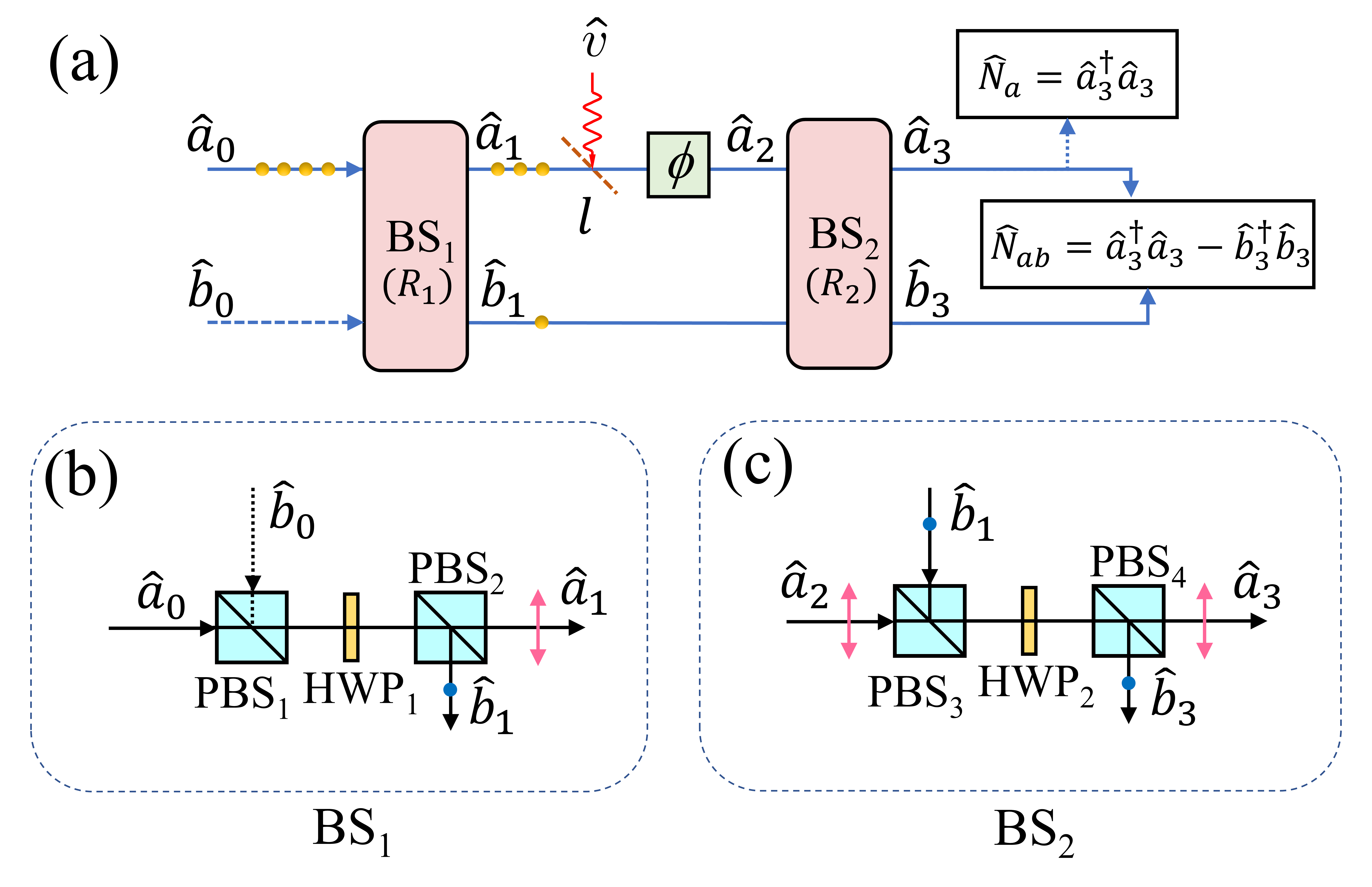
Figure 1: (a) Lossy MZI model with single-intensity detection and difference-intensity detection. The arm $a$ experiences the loss (loss rate: $l$) and phase shift $\phi$. $\hat{a}_{0}$: annihilation operators of coherent state; $\hat{b}_{0},\hat{v}$: annihilation operators of vacuum state. $\hat{a}_{i},\hat{b}_{i}$ $(i=1,2,3)$: annihilation operators for beams at different positions of the interferometer. The yellow balls show the distribution of photons. (b-c) Schematic of beam splitters.BS_1,2: beam splitters with respective reflectivities $R_{1,2}$. PBS: polarization beam splitter; HWP: half-wave plate.

Theory

In Fig. 1(a), We consider an MZI model composed of the two input fields (a coherent field and a vacuum field) and two beam splitters BS_1,2 with reflectivities $R_{1,2}$. An adjustable attenuator with a loss rate of $l$ is placed in a single arm $a$ to simulate the propagation loss (the case of losses on two arms has been discussed in Appendix A.1). The input-output relation of BS₁ is given as

$$\hat{a}_{1}=\sqrt{1-R_{1}}\hat{a}_{0}+i\sqrt{R_{1}}\hat{b}_{0},$$ (1)

$$\hat{b}_{1}=\sqrt{1-R_{1}}\hat{b}_{0}+i\sqrt{R_{1}}\hat{a}_{0},$$

where $\hat{a}_{0}$ and $\hat{b}_{0}$ are the annihilation operators of the coherent and vacuum fields, respectively. We treat the loss as a fictitious beam splitter, $\hat{v}$ is the annihilation operator of the vacuum state introduced by the loss. After experiencing internal loss $l$ and considering a phase shift $\phi$ in the lossy arm $a$, $\hat{a}_{1}$ becomes

$$\hat{a}_{2}=(\sqrt{1-l}\hat{a}_{1}+i\sqrt{l}\hat{v})e^{i\phi}.$$ (2)

The phase shift can be obtained from the interference outputs $\hat{a}_{3},\hat{b}_{3}$ by single-intensity detection or difference-intensity detection 22 . Below, we theoretically analyze the phase sensitivity of MZI with these two detections.

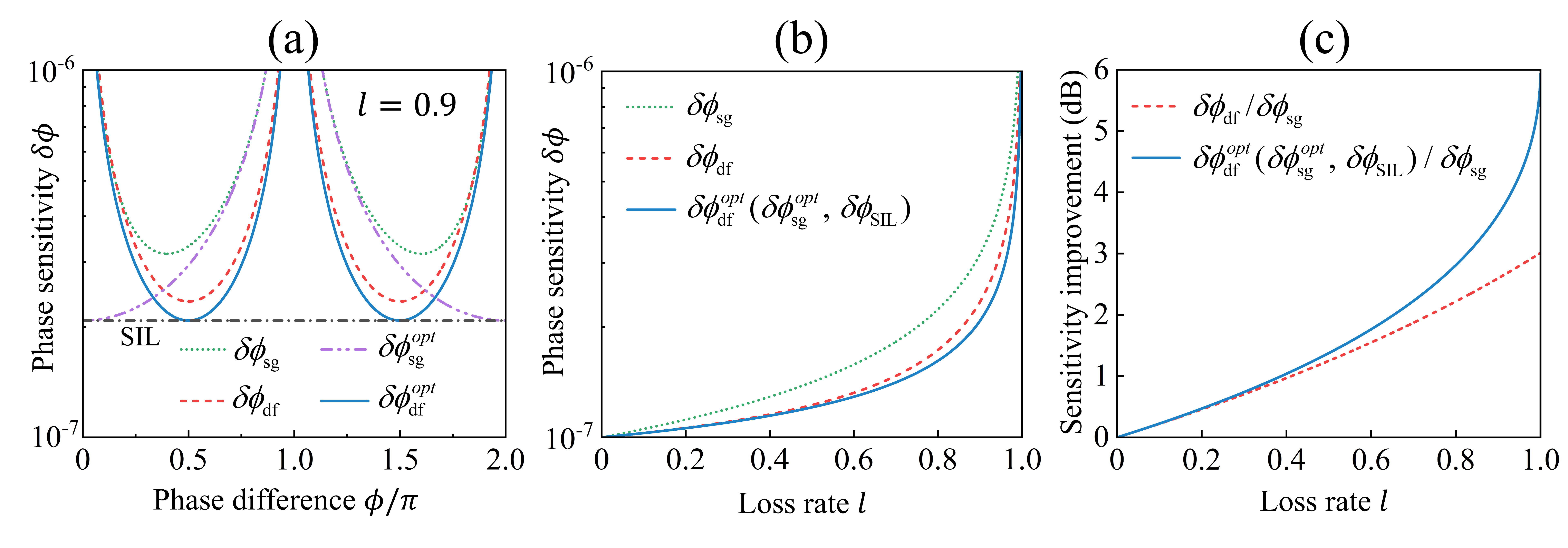
Figure 2: Theoretical optimization analysis of sg- and df-detections. (a) Phase sensitivity of two detections versus phase difference $\phi$ with balanced beam splitting ratios ($\delta\phi_{\text{sg}}$, $\delta\phi_{\text{df}}$) or optimal ones ($\delta\phi_{\text{sg}}^{opt}$, $\delta\phi_{\text{df}}^{opt}$) in MZI. Loss rate $l=0.9$; Photon number $N=10^{14}$. (b) Phase sensitivity $\delta\phi$ as a function of the loss rate $l$. All results are obtained with the respective best phase difference. $\delta\phi_{\text{SIL}}$: sensitivity of standard interferometric limit. (c) Sensitivity improvements are defined as $-20\text{log}_{10}(\delta\phi/\delta\phi_{\text{sg}})$, with the non-optimized sensitivity of sg-detection $\delta\phi_{\text{sg}}$ as the reference. $\delta\phi$ represents $\delta\phi_{\text{df}}$, $\delta\phi_{\text{sg}}^{opt}$, $\delta\phi_{\text{df}}^{opt}$, or $\delta\phi_{\text{SIL}}$. The $\phi_{\text{sg}}^{opt}$, $\delta\phi_{\text{df}}^{opt}$, and $\delta\phi_{\text{SIL}}$ curves overlap together in (b) and (c).

I. Single-intensity (sg) detection

Single-intensity detection only measures $\hat{N}_{a}=\hat{a}_{3}^{{\dagger}}\hat{a}_{3}$ of the output $a_{3}$ using one detector. The phase sensitivity $\delta\phi_{\text{sg}}$ is evaluated as [details see Appendix A.1.1]

$$\delta\phi_{\text{sg}}=\frac{\left\langle\Delta\hat{N}_{a}\right\rangle}{\left|\partial\left\langle\hat{N}_{a}\right\rangle/\partial\phi\right|}=\dfrac{\sqrt{(B-C\cos\phi)N}}{CN\left|\sin\phi\right|},$$ (3)

with

$$B=(1-R_{1})(1-R_{2})(1-l)+R_{1}R_{2},$$ (4)

$$C=2\sqrt{(1-R_{1})(1-R_{2})R_{1}R_{2}(1-l)},$$

where $N$ is the photon number of the coherent optical field $a_{0}$. The optimal phase shift $\phi^{opt}$ and optimal reflectivities $R_{1}^{opt},R_{2}^{opt}$ corresponding to the best phase sensitivity are

$$R_{1}^{opt}=R_{2}^{opt}=\frac{\sqrt{1-l}}{1+\sqrt{1-l}},$$ (5)

$$\phi^{opt}=0,2\pi.$$

With $R_{1}^{opt},R_{2}^{opt}$ and $\phi^{opt}$, we can achieve the optimal sensitivity of sg-detection that is

$$\delta\phi_{\text{sg}}^{opt}=\frac{1+\sqrt{1-l}}{2\sqrt{(1-l)N}},$$ (6)

which depends on the loss rate $l$ and photon number $N$.

II. Difference-intensity (df) detection

Difference-intensity detection measures the intensity difference of two outputs ${a}_{3}$ and ${b}_{3}$, $\hat{N}_{ab}=\hat{a}_{3}^{{\dagger}}\hat{a}_{3}-\hat{b}_{3}^{{\dagger}}\hat{b}_{3}$. The phase sensitivity $\delta\phi_{\text{df}}$ is obtained by (details see Appendix A.1.2)

$${\delta\phi_{\text{df}}=\frac{\left\langle\Delta\hat{N}_{ab}\right\rangle}{\left|\partial\left\langle\hat{N}_{ab}\right\rangle/\partial\phi\right|}=\frac{\sqrt{BN}}{2CN\left|\sin\phi\right|}}.$$ (7)

Different from the sg-detection, the optimal conditions for the best sensitivity of df-detection $\delta\phi_{\text{df}}^{opt}$ are $R_{2}^{opt}=0.5$, $\phi^{opt}$=$\pi/2$. Furthermore, the sensitivity $\delta\phi_{\text{df}}$ with $R_{2}^{opt}$ and $\phi^{opt}$ is given as

$$\delta\phi_{\text{df}}=\sqrt{\frac{1-l+R_{1}l}{4(1-R_{1})R_{1}(1-l)}}\cdot\frac{1}{\sqrt{N}}.$$ (8)

Therefore, the optimal conditions corresponding to the minimum phase sensitivity are

$$R_{1}^{opt}=\frac{\sqrt{1-l}}{1+\sqrt{1-l}},R_{2}^{opt}=0.5,$$ (9)

$$\phi^{opt}=\frac{\pi}{2},\frac{3\pi}{2}.$$

Final optimal sensitivity of df-detection is

$$\delta\phi_{\text{df}}^{opt}=\frac{1+\sqrt{1-l}}{2\sqrt{(1-l)N}}.$$ (10)

$R_{1}^{opt}$ and $\delta\phi_{\text{df}}^{opt}$ are the same as those of sg-detection.

III. Standard interferometric limit (SIL)

Quantum Fisher information (QFI) of a lossy MZI has been discussed in Ref.29 . The QFI results provide the optimal reflectivity $R_{1}$ for the first beam splitter, which is not relevant to the $R_{2}$ for the second beam splitter and the specific detection method. Therefore, there is an optimal phase estimation that can be achieved with the existing loss conditions (losses in two arms:$l_{a},l_{b}$), called standard interferometric limit (SIL). The phase sensitivity of SIL is given by

$$\delta\phi_{\text{SIL}}=\frac{\sqrt{1-l_{a}}+\sqrt{1-l_{b}}}{2\sqrt{(1-l_{a})(1-l_{b})N}}$$ (11)

with the optimal $R_{1}$

$$R_{1}^{opt}=\frac{\sqrt{1-l_{a}}}{\sqrt{1-l_{a}}+\sqrt{1-l_{b}}}.$$ (12)

$R_{1}^{opt}$ and $\delta\phi_{\text{SIL}}$ are the same as optimum cases of sg- and df-detections by setting $l_{a}=l,l_{b}=0$. From Eqs. (6,10,11), it is clear that SIL can be achieved with correct optimization on both detection methods.

V. Analysis

The theoretical comparison of the two detection methods before and after optimization is analyzed in detail in Fig. 2. Fig. 2(a) gives the phase sensitivity with phase differences from 0 to 2$\pi$ when the loss rate is 0.9. The minimum value of $\delta\phi_{\text{df}}$ is smaller than that of $\delta\phi_{\text{sg}}$ with balanced beam splitting ratios, showing the advantage of df-detection in lossy CMZI. After optimizing the beam-splitting ratios, the sensitivity of two methods can reach SIL at their respective optimal phase differences. As shown in Fig. 2(b), the best phase sensitivity of CMZI with df-detection (red dashed line) is always better than that of sg-detection (green dotted line) at all loss rates. Therefore, the df-detection is more loss-tolerant than the sg-detection. More importantly, the best phase difference $\phi^{opt}$ of sg-detection is different before and after optimization, while $\phi^{opt}$ of df-detection is always located at $\pi/2$. This means the optimization of MZI with the df -detection is easier to operate by using phase-locking at $\pi/2$ in practical application.

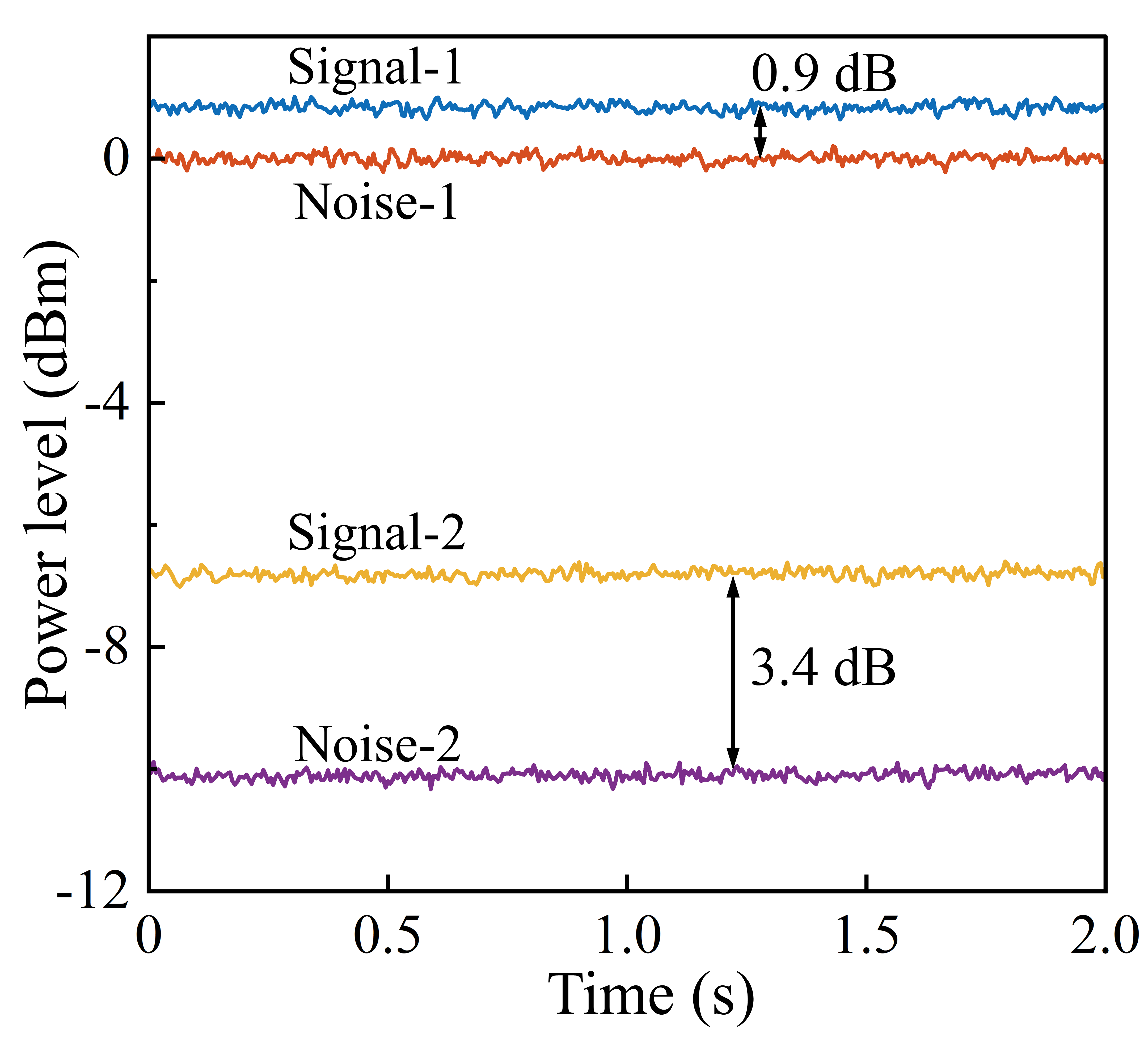
Figure 3: Signal and noise are measured using the df-detection at 1.5 MHz with a spectrum analyzer (SA). 1 and 2 represent the results of MZI with balanced reflectivities ($R_{1}=R_{2}=0.5$) and optimal reflectivities ($R_{1}=0.04,R_{2}=0.5$), respectively. A 2.5 dB signal-to-noise improvement is achieved via $R_{1}$ optimization. SA parameters: 1.5 MHz zero span with a resolution bandwidth (RBW) of 30 kHz and a video bandwidth (VBW) of 30 Hz. Phase difference $\phi$ is locked at $\pi/2$. Loss rate is set to $l=0.998$. Noise-1 is set to 0 dBm as a reference.

In this paper, we focus on sensitivity improvement via reflectivity optimization. The sensitivity with both sg- and df-detections can be improved by utilizing the optimal parameters ($R_{1}^{opt},R_{2}^{opt},\phi^{opt}$) at all loss rates. The optimal sensitivities with two detection schemes, $\delta\phi_{\text{df}}^{opt}$ and $\delta\phi_{\text{sg}}^{opt}$, are exactly the same (solid line in Fig. 2(b)), and are also exactly overlapped with $\delta\phi_{\text{SIL}}$. The sensitivity improvement as a function of loss rate $l$ is given in Fig. 2(c) normalized by CMZI with sg-detection ($\delta\phi_{\text{sg}}$) as a reference in 0 dBm.

The sensitivity improvement increases with the loss. When the loss rate $l$ is close to 1, the sensitivity of CMZI with df-detection is better than that of sg-detection by 3 dB. Furthermore, the optimization of the reflectivities can bring a nearly 6 dB improvement with sg-detection. We choose df-detection in our experiments because the phase difference $\phi^{opt}$ and reflectivity $R_{2}$ only need to be locked at $\pi/2$ and $0.5$ at any loss rate, and the optimal phase sensitivity is consistent with $\delta\phi_{\text{SIL}}$. When the losses change, we simply adjust $R_{1}$ to the optimum value, which facilitates practical applications.

Experiment

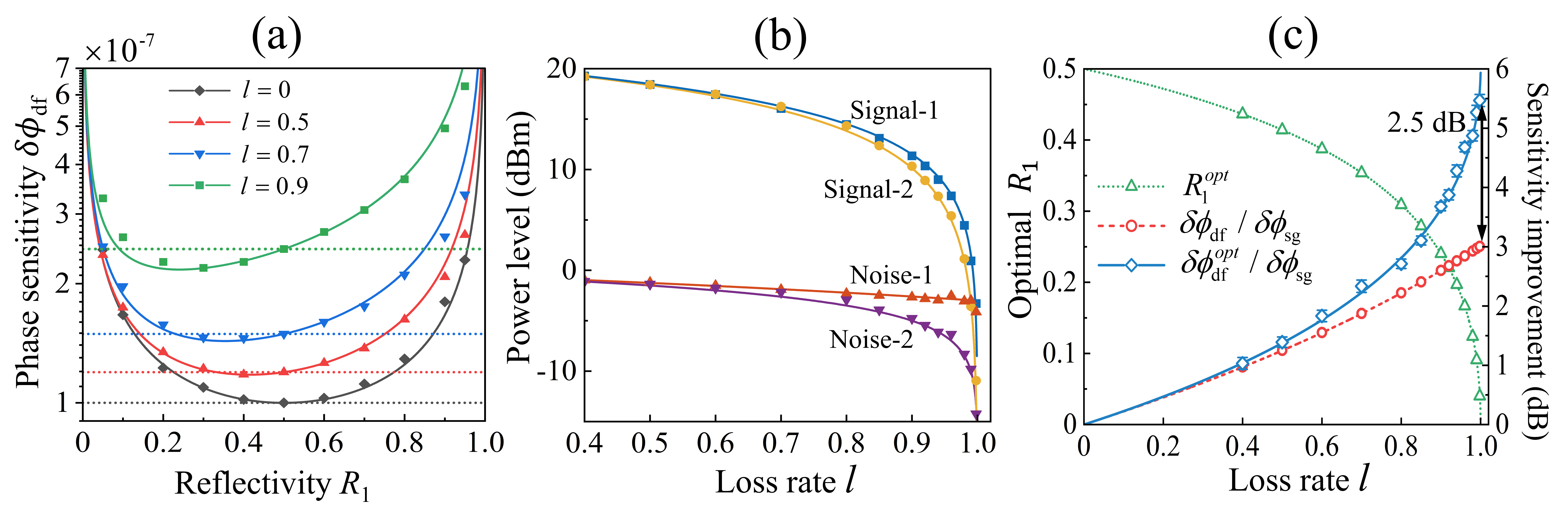
Figure 4: (a) Experimental data of phase sensitivity $\delta\phi$ versus $R_{1}$ at different loss rate $l$. Solid lines: theoretical prediction. Dotted lines: phase sensitivity of MZI with $R_{1}=R_{2}=0.5$. (b) Signal and noise measured with different loss rates $l$ when (1) $R_{1}=0.5$ or (2) $R_{1}=R_{1}^{opt}$. (c) Optimal $R_{1}$ (left axis: dotted line and triangles) and sensitivity improvement (right axis: solid and dashed lines, diamonds and circles) as functions of the loss rate $l$. Lines: theoretical values; Scatters: experimental data. Sensitivity improvements are given with respect to $\delta\phi_{\text{sg}}$. $\delta\phi_{\text{df}}^{opt}$ and $\delta\phi_{\text{df}}$ are the sensitivities of df-detection measured with optimal $R_{1}$ and non-optimal $R_{1}$=0.5, respectively.

In the experiment, coherent light from a semiconductor laser as the optical input field $a_{0}$ of the MZI. BS_1,2 are constructed as shown in Fig. 1(b,c). The input fields $a_{0}$ and $b_{0}$ with respective horizontal and vertical polarizations are combined by a polarization beam splitter (PBS₁) and then divided into two arms after passing through the half-wavelength plate (HWP₁) and PBS₂. The reflectivity $R_{1}$ is continuously adjusted by rotating HWP₁. A smaller $R_{1}$ value means more coherent light passing the loss path. The same design is applied for the BS₂. Considering the optimal conditions of the df-detection, HWP₁ is rotated to a specific degree and HWP₂ is fixed at 22.5^∘ to achieve an adjustable $R_{1}$ and a constant $R_{2}=0.5$. An adjustable attenuator is placed in the signal arm $a$ of the interferometer for continuous simulation of the internal loss rate $l$. Since the output electrical signal of the df-detection is oddly symmetrical at phase difference $\phi=\pi/2$, part of it is used as an error signal for phase-locking (not shown in Fig. 1(a)). The phase difference $\phi$ between two arms is always locked at optimal value $\pi/2$ during the measurement process. A small phase shift $\Delta\phi$ is introduced by a 1.5 MHz-frequency modulation signal using a piezoelectric ceramic mirror. Signal and noise are measured at 1.5 MHz using df-detection by spectrum analyzer when the phase shift is modulated and unmodulated, respectively. As shown in Fig. 3, the signal-1 (blue) and noise-1 (red) curves represent the signal and noise of MZI with balanced $R_{1}$ when $l=0.998$. After optimizing $R_{1}$ to 0.04, the signal-to-noise ratio increased from 0.9 dB to 3.4 dB, although both signal and noise decreased. Finally, the phase sensitivity is obtained from the signal-to-noise conversion (see Appendix.A) with a 2.5 dB sensitivity improvement. To reflect the sensitivity improvement due to reflectivity $R_{1}$ optimization, we continuously measure the sensitivity as a function of $R_{1}$ at different losses ($l=0,0.5,0.7,0.9$) shown in Fig. 4(a), and the results are in excellent agreement with Eq. 8.

This clearly shows that the optimal $R_{1}$ (the $R_{1}$ value at best sensitivity) for lossless MZI is the conventional reflectivity 0.5. The best sensitivity degrades with the increase of the loss rate. Obviously, the loss results in a negative impact on the phase sensitivity. The optimal $R_{1}$ is smaller when the loss rate $l$ is larger. Smaller $R_{1}$ means more photons passing through the lossy arm, which results in degradation of both signal and noise but benefits the sensitivity improvement. This is due to the decay rates of signal and noise being different at different $R_{1}$. The optimal $R_{1}$ is the balance between signal and noise decay. Furthermore, the decay rates of signal and noise also change with the loss rate, resulting in the optimal $R_{1}$ varying with $l$. This point can be seen from Eqs.(6,10) and is also shown in Fig. 4(c). The optimal $R_{1}$ corresponding to the best sensitivity decreases as the loss increases. To further explore the relationship between the sensitivity improvement and the loss rate, we measure the signal and noise with or without optimization of $R_{1}$ at loss rates from 0.4 to 0.998, as shown in Fig. 4(b). The signal and noise both decrease as the loss increases, but the noise after optimization (Noise-2) decreases much faster, especially when the loss rate $l$ approaches 1. Thus, the sensitivity is improved more by optimizing $R_{1}$ at large losses.

In the experiment, we calculate the optimal $R_{1}$ values at different losses and adjust $R_{1}$ experimentally to measure the optimized phase sensitivity ($\delta\phi_{\text{df}}^{opt}$). As shown in Fig. 4(c), the $R_{1}^{opt}$ value decreases with the increase of the loss rate. Compared with the sensitivity of unoptimized df-detection ($\delta\phi_{\text{df}}$), the optimal sensitivity ($\delta\phi_{\text{df}}^{opt}$) is improved at all loss rates and enhanced more at higher loss rate, benefited from the $R_{1}$ optimization. For example, $\delta\phi_{\text{df}^{opt}}$ achieves an optimization of 2.5 dB when l = 0.998, which equates to a 5.5 dB sensitivity improvement compared to the theoretical $\delta\phi_{\text{sg}}$. In general, the experimental results agree with the theoretical predictions well.

Summary and Outlook

In this paper, an MZI with variable beamsplitters is designed and demonstrated to improve the phase sensitivity with the existence of unbalanced losses. We theoretically give the optimal conditions and analyze the optimal phase sensitivity of two detections (sg-detection and df-detection) which both can saturate the optimal sensitivity$\sim$$\delta\phi_{\text{SIL}}$. When the loss rate $l$ is as high as 0.998, a sensitivity improvement of 2.5 dB is achieved in df-detection by optimizing $R_{1}$, which is equivalent to a 5.5 dB improvement in sg-detection. Clearly, in an MZI with balanced 50:50 beam splitters, it is difficult to improve sensitivity with large losses. Such optimization schemes should have a wide range of potential applications when unbalanced losses are unavoidable, e.g. optical hardware for networks, LISA schemes for the detection of gravitational waves, unbalanced MZI for continuous variable entanglement measurements, etc.

Appendix

Appendix A Phase sensitivity

With a small phase shift $\Delta\phi$, the average of measurement operator $\hat{O}$ of MZI can be described as

$$\left\langle\hat{O}(\phi+\Delta\phi)\right\rangle\approx\left\langle\hat{O}(\phi)\right\rangle+\left|\frac{\partial\left\langle\hat{O}\right\rangle}{\partial\phi}\right|\Delta\phi.$$ (a1)

From the above equation, the signal and noise can be written as

$$\text{Signal}=\left|\frac{\partial\left\langle\hat{O}\right\rangle}{\partial\phi}\right|\Delta\phi,\text{Noise}=\left\langle\Delta\hat{O}\right\rangle,$$ (a2)

where $\left\langle\Delta\hat{O}\right\rangle=[\left\langle\hat{O}^{2}\right\rangle-\left\langle\hat{O}\right\rangle^{2}]^{1/2}$ is the standard deviation of $\hat{O}$. $\Delta\phi$ can only be detected when the signal is larger than the noise, therefore

$$\Delta\phi\geqslant\frac{\left\langle\Delta\hat{O}\right\rangle}{\left|\partial\left\langle\hat{O}\right\rangle/\partial\phi\right|}.$$ (a3)

When we modulate the phase shift $\phi$ with a specific frequency signal, a small phase shift $\Delta\phi$ is introduced. Thus, the minimum detectable change in phase shift, called phase sensitivity $\delta\phi$, can be given as

$$\delta\phi=\Delta\phi_{\min}=\frac{\left\langle\Delta\hat{O}\right\rangle}{\left|\partial\left\langle\hat{O}\right\rangle/\partial\phi\right|}=\frac{\text{Noise}}{\text{Signal}}\Delta\phi.$$ (a4)

A.1 Losses in two arms ($l_{a}$, $l_{b}$)

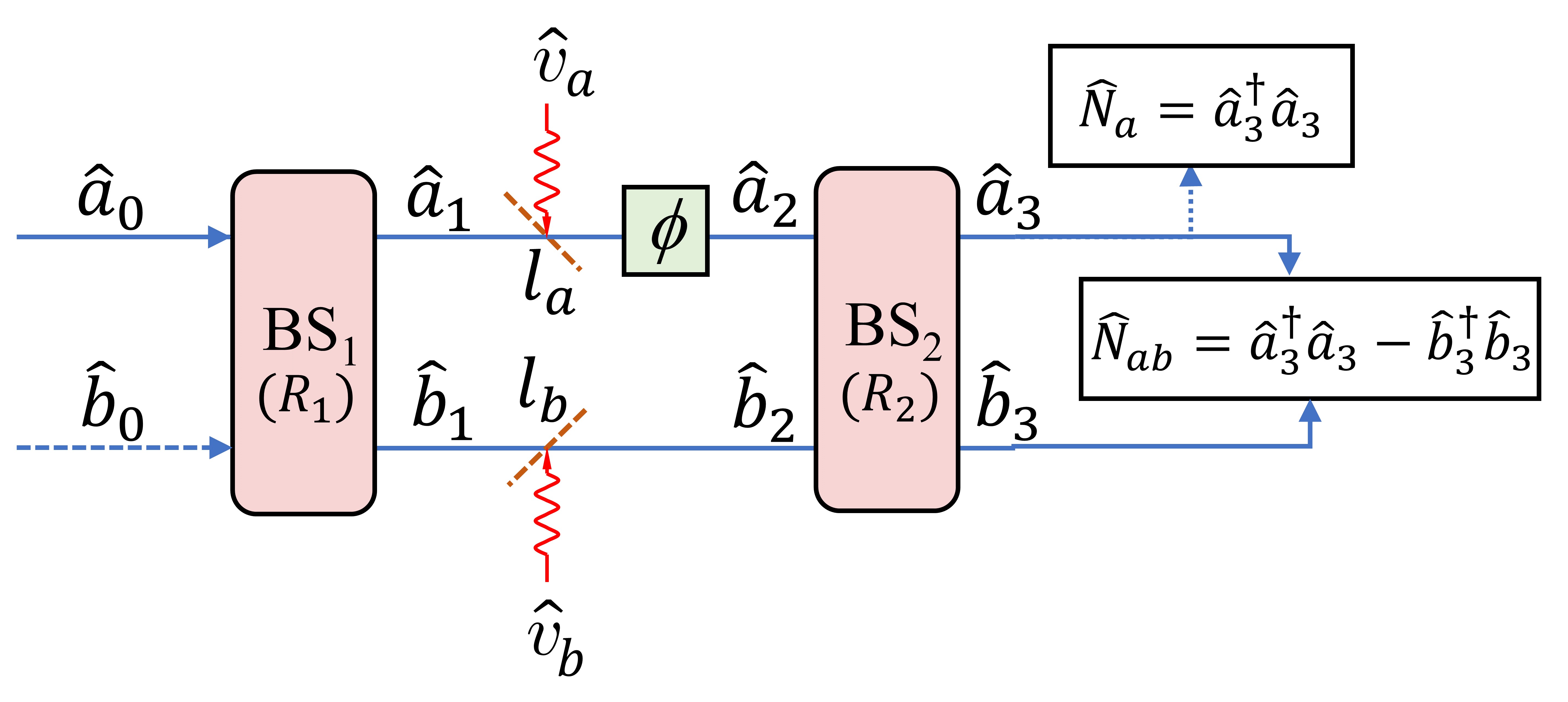
Figure A1: Model of internal losses on two arms of MZI. $l_{a}$,$l_{b}$: loss rates. $\hat{v}_{a},\hat{v}_{b}$: annihilation operators for vacuum fields introduced by losses $l_{a}$,$l_{b}$.

An MZI model with double-arm internal losses ($l_{a}$,$l_{b}$) is illustrated in Fig. A1, which is more general than the simplified model in Fig. 1(a) (only considering single-arm loss $l$ by setting $l_{a}=l,l_{b}=0$). The correspondence between the input and output states is as follows

$$\hat{a}_{3} =\sqrt{1-R_{2}}\hat{a}_{2}+i\sqrt{R_{2}}\hat{b}_{2}$$ (a5)

$$=k_{1}\hat{a}_{0}+k_{2}\hat{b}_{0}+k_{3}\hat{v}_{a}+k_{4}\hat{v}_{b},$$

$$\hat{b}_{3} =\sqrt{1-R_{2}}\hat{b}_{2}+i\sqrt{R_{2}}\hat{a}_{2}$$

$$=h_{1}\hat{a}_{0}+h_{2}\hat{b}_{0}+h_{3}\hat{v}_{a}+h_{4}\hat{v}_{b},$$

where the assumed coefficients are

$$k_{1}=\sqrt{(1-R_{1})(1-R_{2})(1-l_{a})}e^{i\phi}-\sqrt{R_{1}R_{2}(1-l_{b})},$$ (a6)

$$k_{2}=i\sqrt{R_{1}(1-R_{2})(1-l_{a})}e^{i\phi}+i\sqrt{(1-R_{1})R_{2}(1-l_{b})},$$

$$k_{3}=i\sqrt{(1-R_{2})l_{a}}e^{i\phi},$$

$$k_{4}=-\sqrt{R_{2}l_{b}},$$

$$h_{1}=i\sqrt{R_{1}(1-R_{2})(1-l_{b})}+i\sqrt{(1-R_{1})R_{2}(1-l_{a})}e^{i\phi},$$

$$h_{2}=\sqrt{(1-R_{1})(1-R_{2})(1-l_{b})}-\sqrt{R_{1}R_{2}(1-l_{a})}e^{i\phi},$$

$$h_{3}=-\sqrt{R_{2}l_{a}}e^{i\phi},$$

$$h_{4}=i\sqrt{(1-R_{2})l_{b}}.$$

1. Single-intensity detection

When intensity detection is performed at a detector, the signal ($\left|\partial\left\langle\hat{N}_{a}\right\rangle/\partial\phi\right|\Delta\phi$), noise ($\left\langle\Delta\hat{N}_{a}\right\rangle$), and phase sensitivity ($\delta\phi_{\text{sg}}$) can be obtained by the following calculation

$$\left\langle\Delta\hat{N}_{a}\right\rangle=[\left\langle\hat{N}{a}^{2}\right\rangle-\left\langle\hat{N}_{a}\right\rangle^{2}]^{1/2}=\sqrt{(B-C\cos\phi)N},$$ (a7)

$$\left|\partial\left\langle\hat{N}_{a}\right\rangle/\partial\phi\right|=CN\left|\sin\phi\right|,$$

$$\delta\phi_{\text{sg}}=\frac{\left\langle\Delta\hat{N}_{a}\right\rangle}{\left|\partial\left\langle\hat{N}_{a}\right\rangle/\partial\phi\right|}=\frac{\sqrt{B-C\cos\phi}}{C\left|\sin\phi\right|}\cdot\frac{1}{\sqrt{N}},$$

with

$$\left\langle\hat{N}_{a}\right\rangle=\left\langle\hat{a}_{3}^{{\dagger}}\hat{a}_{3}\right\rangle=k_{1}^{\ast}k_{1}N,$$ (a8)

$$\left\langle\hat{N}_{a}^{2}\right\rangle=\left\langle\hat{a}_{3}^{{\dagger}}\hat{a}_{3}\hat{a}_{3}^{{\dagger}}\hat{a}_{3}\right\rangle=(k_{1}^{\ast}k_{1})^{2}N^{2}+k_{1}^{\ast}k_{1}N,$$

$$B=(1-R_{1})(1-R_{2})(1-l_{a})+R_{1}R_{2}(1-l_{b}),$$

$$C=2\sqrt{R_{1}R_{2}(1-R_{1})(1-R_{2})(1-l_{a})(1-l_{b})}.$$

The Phase sensitivity $\delta\phi_{\text{sg}}$ is a function of the parameters $R_{1},R_{2},l_{a},l_{b}$ and $\phi$. From Eq. (a7), we can determine the optimization condition for the minimum phase sensitivity as

$$R_{1}^{opt}=R_{2}^{opt}=\frac{\sqrt{1-l_{a}}}{\sqrt{1-l_{a}}+\sqrt{1-l_{b}}},$$ (a9)

$$\phi^{opt}=\arccos(\frac{B-\sqrt{B^{2}-C^{2}}}{C})=0,2\pi.$$

2. Difference-intensity detection

When using two detectors for difference-intensity detection, the signal, noise and phase sensitivity $\delta\phi_{\text{df}}$ can be expressed as

$$\left\langle\Delta\hat{N}_{ab}\right\rangle=[\left\langle\hat{N}_{ab}^{2}\right\rangle-\left\langle\hat{N}_{ab}\right\rangle^{2}]^{1/2}=\sqrt{BN},$$ (a10)

$$\left|\partial\left\langle\hat{N}_{ab}\right\rangle/\partial\phi\right|=2CN\left|\sin\phi\right|,$$

$$\delta\phi_{\text{df}}=\frac{\left\langle\Delta\hat{N}_{ab}\right\rangle}{\left|\partial\left\langle\hat{N}_{ab}\right\rangle/\partial\phi\right|}=\frac{\sqrt{B}}{2C\left|\sin\phi\right|}\cdot\frac{1}{\sqrt{N}}.$$

with

$$\left\langle\hat{N}_{ab}\right\rangle =\left\langle\hat{a}_{3}^{{\dagger}}\hat{a}_{3}-\hat{b}_{3}^{{\dagger}}\hat{b}_{3}\right\rangle=\left\langle A_{11}\hat{a}_{0}^{{\dagger}}\hat{a}_{0}\right\rangle,$$ (a11)

$$\left\langle\hat{N}_{ab}^{2}\right\rangle =A_{11}^{2}\left\langle\hat{a}_{0}^{{\dagger}}\hat{a}_{0}\hat{a}_{0}^{{\dagger}}\hat{a}_{0}\right\rangle+A_{12}A_{21}\left\langle\hat{a}_{0}^{{\dagger}}\hat{b}_{0}\hat{b}_{0}^{{\dagger}}\hat{a}_{0}\right\rangle$$

$$+A_{13}A_{31}\left\langle\hat{a}_{0}^{{\dagger}}\hat{v}_{a}\hat{v}_{a}^{{\dagger}}\hat{a}_{0}\right\rangle+A_{14}A_{41}\left\langle\hat{a}_{0}^{{\dagger}}\hat{v}_{b}\hat{v}_{b}^{{\dagger}}\hat{a}_{0}\right\rangle$$

$$=A_{11}^{2}N^{2}+(A_{11}^{2}+A_{12}A_{21}+A_{13}A_{31}+A_{14}A_{41})N,$$

$$A_{ij} =k_{i}^{\ast}k_{j}-h_{i}^{\ast}h_{j}(i,j=1,2,3,4).$$

Unlike sg-detection, the phase sensitivity of difference-intensity detection ($\delta\phi_{\text{df}}$) always takes the minimum value at $\phi=\frac{\pi}{2}$ and $R_{2}=0.5$ with reference to Eq. (a12).

$$\frac{\partial(\delta\phi_{\text{df}})}{\partial\phi}\equiv 0|_{\phi=\frac{\pi}{2}},\frac{\partial(\delta\phi_{\text{df}})}{\partial R_{2}}\equiv 0|_{R_{2}=0.5}.$$ (a12)

After setting phase shift $\phi$ to $\frac{\pi}{2}$ and reflectivity $R_{2}$ to $0.5$, the simplified phase sensitivity is

$$\delta\phi_{\text{df}}=\sqrt{\frac{1-l_{a}+R_{1}(l_{a}-l_{b})}{4(1-R_{1})R_{1}(1-l_{a})(1-l_{b})}}\cdot\frac{1}{\sqrt{N}}.$$ (a13)

Using Eq. (a13), we can find the conditions for optimal phase sensitivity

$$R_{1}^{opt}=\frac{\sqrt{1-l_{a}}}{\sqrt{1-l_{a}}+\sqrt{1-l_{b}}},R_{2}^{opt}=0.5,$$ (a14)

$$\phi^{opt}=\frac{\pi}{2},\frac{3\pi}{2}.$$

When both detection methods are under optimal conditions (Eq. a9, Eq. a14), their best phase sensitivities reach SIL.

$$\delta\phi_{\text{df}}^{opt}=\delta\phi_{\text{sg}}^{opt}=\delta\phi_{\text{SIL}}=\frac{\sqrt{1-l_{a}}+\sqrt{1-l_{b}}}{2\sqrt{(1-l_{a})(1-l_{b})N}}.$$ (a15)

The unbalanced loss has the same characteristics for the optimization of sensitivity, whether on a single arm or double arms. For convenience, we consider the case of loss just on a single arm in this paper ($l_{a}=l,l_{b}=0$).

A.2 Measurement

The current of the df-detection is divided into two ways, one as an error signal to lock the phase difference of the MZI at $\pi/2$, and the other for signal measurement.

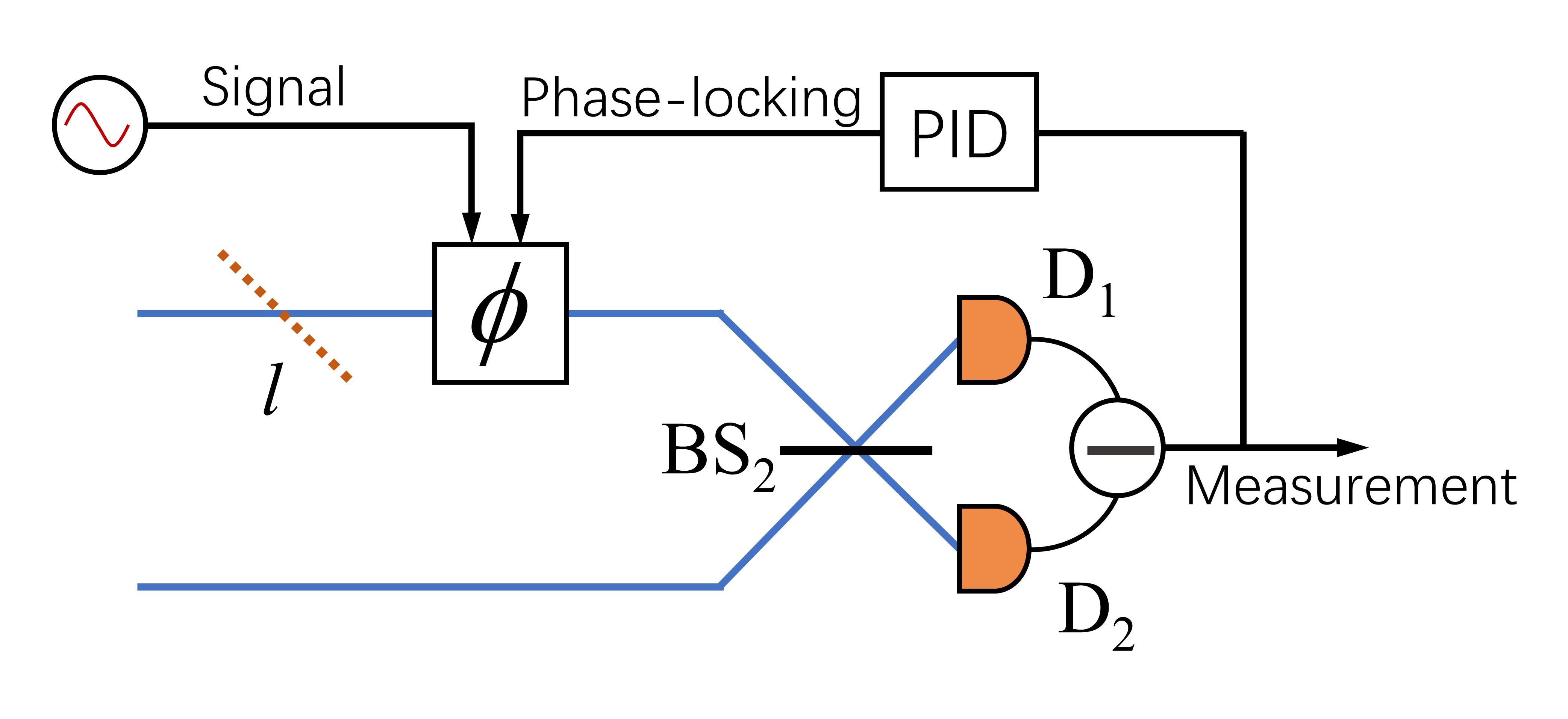
Figure A2: Experimental details. $D_{1}$, $D_{2}$: detectors.

References

- (1) Parameswaran Hariharan. Optical Interferometry, 2e. Elsevier, 2003.
- (2) Chien-ming Wu and Ching-shen Su. Nonlinearity in measurements of length by optical interferometry. Measurement Science and Technology, 7(1):62, 1996.
- (3) Aephraim M. Steinberg, Paul G. Kwiat, and Raymond Y. Chiao. Dispersion cancellation and high-resolution time measurements in a fourth-order optical interferometer. Phys. Rev. A, 45:6659–6665, May 1992.
- (4) M. Fokine, L. E. Nilsson, Å. Claesson, D. Berlemont, L. Kjellberg, L. Krummenacher, and W. Margulis. Integrated fiber mach–zehnder interferometer for electro-optic switching. Opt. Lett., 27(18):1643–1645, Sep 2002.
- (5) Callum M Wilkes, Xiaogang Qiang, Jianwei Wang, Raffaele Santagati, Stefano Paesani, Xiaoqi Zhou, David AB Miller, Graham D Marshall, Mark G Thompson, and Jeremy L O’Brien. 60 db high-extinction auto-configured mach–zehnder interferometer. Optics Letters, 41(22):5318–5321, 2016.
- (6) Matteo G. A. Paris. Entanglement and visibility at the output of a mach-zehnder interferometer. Phys. Rev. A, 59:1615–1621, Feb 1999.
- (7) Chinmoy Taraphdar, Tanay Chattopadhyay, and Jitendra Nath Roy. Mach–zehnder interferometer-based all-optical reversible logic gate. Optics & Laser Technology, 42(2):249–259, 2010.
- (8) Taesoo Kim and Heonoh Kim. Phase sensitivity of a quantum mach-zehnder interferometer for a coherent state input. J. Opt. Soc. Am. B, 26(4):671–675, Apr 2009.
- (9) Jong-Tae Shin, Heo-Noh Kim, Goo-Dong Park, Tae-Soo Kim, and Dae-Yoon Park. The phase-sensitivity of a mach-zehnder interferometer for coherent light. J. Opt. Soc. Korea, 3(1):1–9, Mar 1999.
- (10) Luca Pezzé and Augusto Smerzi. Phase sensitivity of a mach-zehnder interferometer. Phys. Rev. A, 73:011801, Jan 2006.
- (11) Xu Yu, Xiang Zhao, Luyi Shen, Yanyan Shao, Jing Liu, and Xiaoguang Wang. Maximal quantum fisher information for phase estimation without initial parity. Opt. Express, 26(13):16292–16302, Jun 2018.
- (12) R. Demkowicz-Dobrzanski, U. Dorner, B. J. Smith, J. S. Lundeen, W. Wasilewski, K. Banaszek, and I. A. Walmsley. Quantum phase estimation with lossy interferometers. Phys. Rev. A, 80:013825, Jul 2009.
- (13) Rafal Demkowicz-Dobrzański, Marcin Jarzyna, and Jan Kołodyński. Quantum limits in optical interferometry. Progress in Optics, 60:345–435, 2015.
- (14) AD Parks, SE Spence, JE Troupe, and NJ Rodecap. Tripartite loss model for mach-zehnder interferometers with application to phase sensitivity. Review of scientific instruments, 76(4):043103, 2005.
- (15) Jan Kołodyński and Rafał Demkowicz-Dobrzański. Phase estimation without a priori phase knowledge in the presence of loss. Phys. Rev. A, 82:053804, Nov 2010.
- (16) Matthew Wescott, Guangzhou Chen, Yanyun Zhang, Brian G Bagley, and Robert T Deck. All-optical combiner-splitter and gating devices based on straight waveguides. Applied Optics, 46(16):3177–3184, 2007.
- (17) Arpita Srivastava and S Medhekar. Switching of one beam by another in a kerr type nonlinear mach–zehnder interferometer. Optics & Laser Technology, 43(1):29–35, 2011.
- (18) O Glöckl, Ulrik L Andersen, S Lorenz, Ch Silberhorn, N Korolkova, and Gerd Leuchs. Sub-shot-noise phase quadrature measurement of intense light beams. Optics Letters, 29(16):1936–1938, 2004.
- (19) Xiaolong Su, Aihong Tan, Xiaojun Jia, Qing Pan, Changde Xie, and Kunchi Peng. Experimental demonstration of quantum entanglement between frequency-nondegenerate optical twin beams. Optics Letters, 31(8):1133–1135, 2006.
- (20) Gregor Weihs, Michael Reck, Harald Weinfurter, and Anton Zeilinger. All-fiber three-path mach–zehnder interferometer. Optics Letters, 21(4):302–304, 1996.
- (21) Shane L. Larson, William A. Hiscock, and Ronald W. Hellings. Sensitivity curves for spaceborne gravitational wave interferometers. Phys. Rev. D, 62:062001, Aug 2000.
- (22) R Demkowicz-Dobrzański. Multi-pass classical vs. quantum strategies in lossy phase estimation. Laser Physics, 20(5):1197–1202, 2010.
- (23) Brendon L Higgins, Dominic W Berry, Stephen D Bartlett, Howard M Wiseman, and Geoff J Pryde. Entanglement-free heisenberg-limited phase estimation. Nature, 450(7168):393–396, 2007.
- (24) BL Higgins, DW Berry, SD Bartlett, MW Mitchell, HM Wiseman, and GJ Pryde. Demonstrating heisenberg-limited unambiguous phase estimation without adaptive measurements. New Journal of Physics, 11(7):073023, 2009.
- (25) D. W. Berry, B. L. Higgins, S. D. Bartlett, M. W. Mitchell, G. J. Pryde, and H. M. Wiseman. How to perform the most accurate possible phase measurements. Phys. Rev. A, 80:052114, Nov 2009.
- (26) Vinzenz Wand, Johanna Bogenstahl, Claus Braxmaier, Karsten Danzmann, Antonio Garcia, Felipe Guzmán, Gerhard Heinzel, Jim Hough, Oliver Jennrich, Christian Killow, et al. Noise sources in the ltp heterodyne interferometer. Classical and Quantum Gravity, 23(8):S159, 2006.
- (27) Markus Otto, Gerhard Heinzel, and Karsten Danzmann. Tdi and clock noise removal for the split interferometry configuration of lisa. Classical and Quantum Gravity, 29(20):205003, 2012.
- (28) R. Demkowicz-Dobrzanski, U. Dorner, B. J. Smith, J. S. Lundeen, W. Wasilewski, K. Banaszek, and I. A. Walmsley. Quantum phase estimation with lossy interferometers. Phys. Rev. A, 80:013825, Jul 2009.
- (29) J J Cooper and J A Dunningham. Towards improved interferometric sensitivities in the presence of loss. New Journal of Physics, 13(11):115003, nov 2011.
- (30) Stefan Ataman, Anca Preda, and Radu Ionicioiu. Phase sensitivity of a mach-zehnder interferometer with single-intensity and difference-intensity detection. Phys. Rev. A, 98:043856, Oct 2018.