Engineering a Distributed-Memory
Triangle Counting Algorithm

Abstract

Counting triangles in a graph and incident to each vertex is a fundamental and frequently considered task of graph analysis. We consider how to efficiently do this for huge graphs using massively parallel distributed-memory machines. Unsurprisingly, the main issue is to reduce communication between processors. We achieve this by counting locally whenever possible and reducing the amount of information that needs to be sent in order to handle (possible) nonlocal triangles. We also achieve linear memory requirements despite superlinear communication volume by introducing a new asynchronous sparse-all-to-all operation. Furthermore, we dramatically reduce startup overheads by allowing this communication to use indirect routing. Our algorithms scale (at least) up to 32 768 cores and are up to 18 times faster than the previous state of the art.

I Introduction

Graphs are a universally used abstraction to describe relations between objects and thus a key to many applications of computers. With the big-data aspect of the information age, it is therefore clear that processing very large graphs quickly and efficiently is an increasingly important problem. For example, the largest social network, Facebook, had over 2.7 billion active users in the fourth quarter of 2020 [2], and the Common Crawl 2012 web hyperlink graph [3] consists of over 100 billion edges and requires 350GB of memory in uncompressed form. A description of the neural connections of the human brain would have about 10 billion vertices (neurons) and 100 trillion edges (synapses). The need to use supercomputers for processing such large networks is widely recognized as witnessed by the popularity of the Graph 500 benchmark [4]. However, the number of graph problems that can be handled efficiently with many thousands of processing elements (PEs) is quite limited so far. Graph 500 concentrates mostly on breadth-first search (BFS) on a single kind of input that is very easy for BFS.

In this paper we want to improve this situation for one of the most widely used graph-analysis problems – triangle counting. Given an undirected graph $G=(V,E)$, we are looking for the number of sets $\{u,v,w\}\subseteq V$ such that these three vertices are mutually connected in $E$. Since triangles can be very non-uniformly distributed over that graph, one often also wants to know the number of triangles incident to each vertex – normalized to the range $[0,1]$. This is known as the local clustering coefficient (LCC).

Triangles are the smallest non-trivial complete subgraph and often indicative of dense regions of the graph. Therefore, the problem has numerous applications in analyzing complex networks such as social graphs [6] but is also applicable in practice. Becchetti et al. [7] show that analyzing the distribution of the local clustering coefficient may be used to detect spam pages on the web, and Eckmann and Moses [8] identify common topics of web pages using triangle counting. Other applications include database query optimizations [9] and link recommendation [10].

After introducing basic concepts in Section II, we discuss previous approaches in Section III. Our algorithms are described in Section IV and evaluated in Section V. Section VI summarizes the results and outlines possible future work.

Contributions

• All triangles that can be found locally are found locally.

• Only cut edges need to be communicated.

• Linear memory requirements using an asynchronous sparse all-to-all algorithm.

• Fast and highly scalable MPI code.

• Better scalability by indirect communication.

• Extensive experiments with large real-world inputs and massive generated graphs from several families of inputs.

• Comparison with state-of-the art competitors shows up to 18$\times$ better performance for large configurations.

• Generalization to exact and approximate computation of local clustering coefficients.

II Preliminaries

In this section we introduce the basic concepts and notations used in this work. We further provide details of the underlying machine model.

II-A Basic Definitions

We consider undirected graphs $G=(V,E)$ where $V=\{0,\ldots,n-1\}$ and $E\subseteq\binom{V}{2}$ are the sets of vertices and edges, respectively. G has $n=|V|$ vertices and $m=|E|$ edges. For a given vertex $v\in V$ let $N_{v}(G)=\{u\in V\mid\{u,v\}\in E\}$ denote the neighborhood of $v$. The degree of $v$ is $d_{v}\coloneqq|N_{v}(G)|$. If the considered graph $G$ is clear from the context, we simply write $N_{v}$ instead of $N_{v}(G)$.

Two vertices $u,v\in V$ are called adjacent if the edge $\{u,v\}\in E$ exists. An edge $e\in E$ is incident to a vertex $v\in V$ if $v\in e$. The vertices incident to an edge are called endpoints.

For $V^{\prime}\subseteq V$ we define the induced subgraph $G(V^{\prime})=(V^{\prime},E^{\prime})$ of $G$, where $E^{\prime}\coloneqq\{\{u,v\}\in E\mid u\in V^{\prime}\land v\in V^{\prime}\}$. For a set of three distinct vertices $u,v,w\in V$, we call the induced subgraph $G(\{u,v,w\})$ a triangle if and only if it is complete, i.e., each edge $\{u,v\},\{v,w\},\{w,u\}$ exists.

Most triangle counting algorithms depend on orienting undirected graphs, to prevent redundant counting of triangles. This is accomplished by using a total ordering $\prec$ on the vertices. Each edge is directed from the lower to higher ranked vertex. With respect to a total ordering $\prec$, we define the outgoing neighborhood of $v\in V$ as $N_{v}^{+}(G)\coloneqq\{u\in V\mid\{v,u\}\in E\land v\prec u\}$ and the incoming neighborhood as $N_{v}^{-}(G)\coloneqq N_{v}(G)\setminus N_{v}^{+}(G)$. We write a directed edge as an (ordered) tuple $(u,v)$ if $u\prec v$. We define the out-degree $d_{v}^{+}$ of a vertex $v\in V$ as $d_{v}^{+}\coloneqq d_{v}^{+}(G)\coloneqq|N_{v}^{+}(G)|$. As before, we do not mention the considered graph explicitly if it is clear from the context. We call each pair of directed edges $(v,u)$, $(v,w)$ a wedge. A naive triangle counting algorithm would be to enumerate all wedges and check if a closing edge $(u,w)$ or $(w,u)$ exists.

II-B Machine Model and Input Format

We consider a system consisting of $p$ processing elements (PEs) numbered $P_{0},\ldots,P_{p-1}$, which are connected via a network with full-duplex, single-ported communication. Sending a message of length $\ell$ from one PE to another takes time $\alpha+\beta\ell$, where $\alpha$ is the time required to initiate a connection and $\beta$ the subsequent transmission time for sending one machine word. Let the communication volume denote the total number of machine words sent between processors.

We assume that input graphs are stored in the adjacency array format, which stores the set of neighbors $N_{v}$ for each vertex $v$ using two arrays in a compressed form. We use 1D partitioning, which means that each $P_{i}$ is assigned a vertex set $V_{i}$, where all sets $V_{i}$ are disjoint and $V=\bigcup_{i=0}^{p-1}V_{i}$. $P_{i}$ stores the neighborhoods for a subsequence $V_{i}$ of the vertices $\{0,\ldots,n-1\}$. A vertex is called local to $P_{i}$ if it lies in $V_{i}$. For a vertex $v$ the rank is defined as $\operatorname{rank}(v)=i:\Leftrightarrow v\in V_{i}$. We assume that processor $P_{i}$ only has access to vertices in $V_{i}$ and their neighborhoods.

In addition to that we assume that the vertices are globally ordered among the processors by vertex ID. This means that if $\text{rank}(v)<\text{rank}(w)$ for vertices $v\in V_{i}$, $w\in V_{j}$, $i\neq j$ then $w$ has a higher ID than $v$.

Vertices $u$ which are contained in a neighborhood $N_{v}$ for a vertex $v\in V_{i}$, but are not local to $P_{i}$ are called ghost vertices. Local vertices which are adjacent to at least one ghost vertex are called interface vertices. An edge connecting two vertices $v\in V_{i}$, $w\in V_{j}$, $i\neq j$ is called cut edge. We define the cut graph $\partial G$ as the graph only consisting of cut edges, i.e., $\partial G\coloneqq(V,E^{\prime})$, where $E^{\prime}\coloneqq\{{u,v}\in E\mid u\in V_{i},v\in V_{j},i\neq j\}$. For processor $P_{i}$ let $\overline{V_{i}}\coloneqq V_{i}\cup\bigcup_{v\in V_{i}}N_{v}$ denote the set of all local vertices and ghost vertices and let $\partial V_{i}\coloneqq\overline{V_{i}}\setminus V_{i}$ denote the set of ghost vertices.

An example of the terminology used is given in Fig. 1.

Figure 1: Example of the various vertex types for the local graph view from $P_{i}$. The edges and vertices colored in gray are not visible to $P_{i}$.

III Related Work

With growing size of real world input instances, there was a correspondingly rising need for efficient triangle counting algorithms. A large variety of approaches has been proposed, tailored to different models of computation. As for sequential algorithms, Schank’s Ph.D. thesis [11] and a more recent work by Ortmann and Brandes [12] give an extensive overview.

Almost all triangle counting algorithms derive from a single sequential base algorithm, which is often referred to as EdgeIterator. It iterates over all edges $\{u,v\}$ in the graph and intersects the neighborhoods of both endpoints. This counts each triangle three times, once from each contained edge. A practical formulation called compact-forward which avoids redundant counting is attributed to Latapy [13]. The algorithm orients the undirected input graph using a degree-based (total) ordering defined as follows: For $u,v\in V$

$$u\prec v\Leftrightarrow\begin{cases}d_{u}<d_{v}&\text{if }d_{u}\neq d_{v}\\ u<v&\text{if }d_{u}=d_{v}\text{\;.}\end{cases}$$

By only considering outgoing neighborhoods, this avoids finding duplicate triangles and also reduces the overall work, because the out-degree of high-degree vertices is reduced. Pseudocode is given in Algorithm 1.

1

2$T\leftarrow 0$

3 for $v\in V$ do

4      for $u\in N_{v}^{+}$ do

5            $T\leftarrow T+|N_{v}^{+}\cap N_{u}^{+}|$

6            

7      

Algorithm 1 EdgeIterator

The set intersection relies on the neighborhoods being sorted. It is implemented using a procedure similar to the merge phase of merge sort.

III-A Parallel Algorithms

Even carefully tuned sequential algorithms are not enough for today’s massive problem instances. To deal with large inputs, one has to exploit processor and memory parallelism.

III-A1 Shared Memory

On a shared memory machine, EdgeIterator may be easily parallelized. As all set intersections in line 1 are independent of each other they may be carried out in parallel and lock-free, as each thread has random access to the whole graph and does not modify it. Shun and Tangwongsan [14] propose a parallel version of EdgeIterator, where the loops in lines 2-2 over vertices $v\in V$ and vertices $u\in N_{v}^{+}$ are executed in parallel. Dhulipala, Shun and Blelloch [15] extend this approach to work on large compressed graphs. They also parallelize the set intersection.

Other shared memory implementations [16, 17] share the same main idea with Shun and Tangwongsan’s algorithm: They are based on variants of EdgeIterator and execute the two outer loops of the algorithms in parallel.

Green et al. [18] use a different approach. Instead of parallelizing on node level, they iterate over all local edges in parallel and intersect the neighborhoods of the endpoints. They estimate the work required per edge and statically partition the edge list into chunks of equal work. They report that if not taking the partitioning step into account, this approach outperforms the node-centric parallelization strategy.

III-A2 Distributed Memory

While triangle counting is easily parallelized on shared memory machines, the availability of systems with high number of processors and sufficient amount of memory for large graphs is still limited today. Distributed memory machines provide us with a large total amount of memory and abundant parallelism. Under the assumption that the graph is 1D partitioned as described in Section II-B, EdgeIterator can be adapted to this distributed setting as shown in Algorithm 2. When processing a local edge $(v,u)$ the local neighborhoods are intersected as before, but when a cut edge is encountered, the neighborhood $N_{v}^{+}$ of $v$ is sent to the local rank $P_{j}$ of $u$, which then performs the set intersection upon receiving the message. The total number of triangles in the graph is then obtained by reducing over the local triangle counts. Firstly, consider that $P_{i}$ processes two edges $(v,u),(v,u^{\prime})$ with $\operatorname{rank}(u)=\operatorname{rank}(u^{\prime})\neq\operatorname{rank}(v)$. Then $N_{v}^{+}$ would be sent to PE $\operatorname{rank}(u)$ twice. Arifuzzaman et. al [19] address this issue and ensure that each neighborhood is only sent to each PE once by exploiting the sortedness of vertex neighborhoods and require only $\operatorname{\mathcal{O}}(|V_{i}|)$ additional memory per PE.

1 $T_{i}\leftarrow 0$

2 for $v\in V_{i}$ do

3      for $u\in N_{v}^{+}$ do

4            if $u\in V_{i}$ then  $T_{i}\leftarrow T_{i}+|N_{v}^{+}\cap N_{u}^{+}|$

5             else  send $((v,u),N_{v}^{+})$ to $P_{\text{rank}(u)}$

6            

7      

8on receive $((v,u),N_{v}^{+})$ do

9       $T_{i}\leftarrow T_{i}+|N_{v}^{+}\cap N_{u}^{+}|$

10      

11$T\leftarrow\textnormal{{Reduce(}}\textnormal{\emph{$T_{i}$, {{SUM}}}}\textnormal{{)}}$

Algorithm 2 Distributed-memory EdgeIterator

Still, their approach sends many small messages, which may lead to high startup overheads. Ghosh et al. [20] address this by aggregating messages and then finally perform a single all-to-all collective operation. Because they only use a single communication step and never empty the buffer, it may require memory superlinear in the input size.

There also exist distributed algorithms based on matrix multiplication on the adjacency matrix, but it is shown that they only scale up to a couple of hundred PEs [21, 22].

Suri and Vassilvitskii [23] describe two distributed algorithms using the popular MapReduce framework [24] which are both based on EdgeIterator. Park et al. [25] further improve this algorithm, but all algorithms produce large amounts of intermediate data by replicating the input graph and in turn require a lot of communication during the shuffle phase, which hinders scalability [26, 25].

Pearce et al. [27, 28, 29] present a triangle counting algorithm using their distributed vertex-centric framework HavoqGT. On the degree-oriented graph they generate all open wedges $(u,v,w)$ for each vertex $v\in V$, i.e., all pairs of outgoing neighbors $\{u,w\}\in\binom{N_{v}^{+}}{2}$, and create new vertex visitor for these neighbors, which then check for a closing edge $(u,w)$ or $(w,u)$. They partition the neighborhoods of high-degree vertices among multiple PEs and also employ message aggregation. To reduce the number of messages, they first aggregate messages at node level and then reroute them to other compute nodes.

There exist algorithms which avoid communication entirely during the counting phase by replicating complete neighborhoods of ghost vertices during preprocessing [30, 31]. This basically offloads the communication done by other approaches to the preprocessing phase and requires superlinear memory to store the replicated vertex neighborhoods. This limits the overall scalability for large inputs [19].

III-B Approximative Algorithms

For many applications it suffices to only approximate the number of triangles instead of determining the exact result. Approximation algorithms may reduce both the time and memory requirements of triangle counting when an exact result is not required. Tsourakakis et al. [32] introduce Doulion, an edge-sampling-based approximation algorithm that reduces the input size. Instead of sampling edges independently, Pagh and Tsourakakis [33] achieve better approximations by coloring vertices independently and only considering the graph of edges where both endpoints have the same color. Both approaches require a (distributed) triangle counting algorithm as a black box to count the triangles in the reduced graph and scale the result accordingly to obtain an approximation. There also exist semi-streaming algorithms for approximating triangle counts [9, 34].

III-C Miscellaneous

For a broader overview on various other specialized algorithms, we refer the reader to the survey by Al Hasan and Dave [35]. While we focus on message passing based approaches for distributed-memory machines there has also been a lot of work using other models of computation. GPU algorithms [36, 37, 30, 38] focus on parallelizing the set intersection operation using binary search based approaches, which are more suitable to be implemented on GPUs than merge-based approaches. The external memory algorithm by Chu and Cheng [39] uses a locality aware contraction technique which is similar to ours. They use it to load chunks of the input graph from disk, count local triangles, remove internal edges and write the contracted graph chunk back to disk. This is repeated until the whole contracted graph fits into main memory. The advances in GPU and external settings are orthogonal to our approach, because they may be used to count local triangles if each PE is equipped with a GPU or the main memory is limited. Our proposed communication reduction techniques may still be employed.

IV Our Algorithms

We identify reducing communication as one of the key challenges for designing a scalable distributed memory triangle counting algorithm. Recall that sending a single message of length $\ell$ takes time $\alpha+\beta\ell$ in the full-duplex model of communication.

We can therefore reduce communication by addressing two parts of this communication model: By limiting the number of messages and reducing the total startup overhead or by reducing the total communication volume. In this section we present two algorithms which address both.

Ditric (Distributed Triangle Counting) employs message aggregation with linear memory requirements and introduces a network agnostic indirect communication protocol.

Cetric (the communication-efficient variant of Ditric) builds upon this, exploits locality and uses graph contraction such that the communication volume is only dependent on the structure of the cut graph. In section IV-E we show how we can reduce communication even more when an approximation of the triangle count is acceptable.

IV-A Message Aggregation

Figure 2: Running time of the basic distributed algorithm on friendster with and without message aggregation.

As already mentioned in Section III-A2, a direct adaptation of EdgeIterator to a distributed system leads to a high number of messages between PEs. To reduce the startup overhead required for sending a message it is feasible to aggregate multiple small messages designated for the same receiver into a single one.

An example how message aggregation improves on scalability is shown in Fig. 2, where we compare the running time of distributed EdgeIterator with and without message aggregation enabled on the friendster graph.

A challenge for distributed triangle counting is that the total communication volume is superlinear in the input size, because each neighborhood may be sent to multiple other PEs. This is a particular issue when using message aggregation since local buffers can already overflow when just one PE needs to send too many messages.

Our algorithm Ditric uses a dynamically buffered message queue to solve this problem. Let $\delta$ be the threshold upon which the buffer should be emptied. Each PE maintains a hash-map of buffers $B_{j}$ as a dynamic array for each communication partner $P_{j}$. If a send operation of the neighborhood of a vertex $v$ to PE $P_{j}$ is issued, we append the neighborhood to the buffer $B_{j}$. If this operation results in the overall buffer size $B=\sum_{j=0}^{p-1}|B_{j}|$ to become greater than the threshold $\delta$, we send all $B_{j}$ to their corresponding receiver PEs. We do this by using double buffering: We replace each $B_{j}$ with an empty buffer and pass the full buffer to the MPI runtime by issuing a non-blocking send operation. While the send operation is carried out, we can continue writing messages to the now empty buffer $B_{j}$ and only block in the unlikely event that the second buffer overflows while the first buffer has not been completely sent yet.

Each PE continuously polls for incoming messages and processes them.

By setting $\delta\in\operatorname{\mathcal{O}}(|E_{i}|)$ we ensure that the memory required per PE never exceeds the local input size.

IV-B Indirect Message Delivery

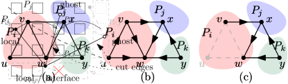
Figure 3: Grid-based indirect message delivery in Cetric.

Message aggregation helps to reduce the startup overhead when a PE sends many small neighborhoods to another communication partner. If a PE owns a high-degree vertex, it has to send and receive many small vertex neighborhoods from/to different communication partners. We propose a simple grid-based indirection scheme, which, combined with aggregation, allows to reduce the communication load.

We therefore arrange the PEs in a logical two-dimensional grid as shown in Fig. 3, and call the PE located in row $i$ and column $j$ $P_{i,j}$. When this PE wants to send a message to $P_{k,l}$, it first sends it along the processor row to the so called proxy PE, $P_{i,l}$. The proxy then forwards the message to $P_{k,l}$ along the processor column.

To give an intuition on how this improves message flow, consider the extreme case that all PEs want to send a message of size $1$ to a single destination PE. Without message indirection, this PE has to receive $p$ messages, therefore requiring time $p(\alpha+\beta)$. If indirection is employed, we double the overall communication volume, but each PE only has $\sqrt{p}$ peers. This results in a overall communication time of $\operatorname{\mathcal{O}}(\sqrt{p}(\alpha+\beta))+p\beta$. This especially comes into play for large values of $p$.

Since each PE maintains a message queue, all messages from a processor row designated to $P_{k,l}$ get aggregated at the proxy. Using a threshold on the message queue as described before, we can still guarantee that each PE only requires $\operatorname{\mathcal{O}}(|E_{i}|)$ space for aggregating messages.

If the number of PEs $p$ is not a square number, we arrange the PEs in a rectangular grid with $\lfloor\sqrt{p}+\frac{1}{2}\rfloor$ columns (i.e., we round to the nearest integer). The last row may not be completely filled. Suppose that $P_{i^{\prime},j^{\prime}}$ wants to send a message to $P_{k,l}$ as depicted in Fig. 3. Then the logical proxy does not exist. We therefore transpose the last row and append it as a column to the right side of the grid and then choose the proxy along the row as described before. Note that this is only necessary when sending from $P_{i^{\prime},j^{\prime}}$ to $P_{k,l}$ and not in the other direction.

While this is somewhat similar to the indirect communication approach used in  [29], our grid-based redirection scheme is network-topology agnostic.

IV-C Exploiting Locality

We now propose a variant of Ditric called Cetric, a contraction based two-phase algorithm which counts triangles locally without using communication whenever possible. The total communication volume of our algorithm is proportional to the size of the contracted graph consisting only of cut edges.

We observe that each triangle $\{u,v,w\}$ in the input graph falls into one of the following categories: If all vertices are local to a single processor $P_{i}$, , i.e., if $u,v,w\in V_{i}$, we call it a type 1 triangle. If any vertex $u\in V_{j}$, $j\neq i$ and both other vertices $v,w\in V_{i}$, we call it a type 2 triangle. If each vertex in the triangle is local to a distinct processor, we call it a type 3 triangle. The different triangle types are depicted in Fig. 4a).

Note that any type 1 triangle may always be found without communication, as all edges of the triangle are “known” to a single PE. While this is also true for type 2 triangles, the basic distributed edge iterator algorithm introduced in section III-A2 does not leverage this due to the orientation of the edges. Consider the type 2 triangle $\{v,w,x\}$ in Fig. 4b). When PE $P_{i}$ examines edges $(v,w)$ the triangle is not found, because the algorithm only intersects outgoing neighborhoods. The triangle is only found by $P_{j}$ after $N_{v}^{+}$ has been sent by $P_{i}$. While this could be fixed by including the in- and outgoing neighborhoods of interface vertices in the set intersection, this would undo the effects of degree orientation, which reduces the out-degree of high-degree vertices.

We propose a two-phase algorithm which finds all type 1 and type 2 triangles using only locally available information while preserving degree orientation. We give a high level description of this approach in Algorithm 3.

Our algorithm leverages this observation by using two phases. In the local phase our algorithm works on the expanded local graph which consists of the set vertex set $\overline{V_{i}}=V_{i}\cup\partial V_{i}$, i.e., all local vertices and ghosts, and all edges which have at least one endpoint in $V_{i}$. Note that constructing this graph requires no communication, as it only consists of edges incident to local vertices. It is easy to see that running any sequential triangle counting algorithm on the expanded graphs yields all type 1 and type 2 triangles.

After the local phase we apply a contraction step, which removes all non-cut edges from the graph as depicted in Fig. 4c).

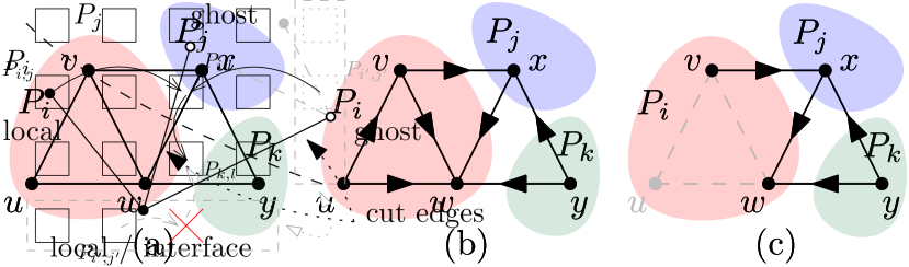
Figure 4: The main idea behind Cetric. (a) shows the different triangle types, $\{u,v,w\}$ is a type 1 triangle, $\{v,w,x\}$ a type 2 triangle and $\{w,x,y\}$ a type 3 triangle. (b) The edges are oriented towards high degree vertices. (c) After the local phase, all non cut edges can be removed from the graph.

In the global phase, we can then use Ditric or any other distributed algorithm on the contracted cut graph to count the remaining type 3 triangles.

1

// Preprocessing (see sec. IV-D)

2 exchange_ghost_degree()

3 $T_{i}\leftarrow 0$

4 foreach $v\in V_{i}$ do $A(v)\leftarrow\{x\in N_{v}\mid x\succ v\}$

5 foreach $v\in\partial V_{i}$ do $A(v)\leftarrow\{x\in N_{v}\mid x\succ v\land x\in V_{i}\}$

// Local Phase

6 foreach $v\in V_{i}\cup\partial V_{i}$ do

7       foreach $u\in A(v)$ do

8             $T_{i}\leftarrow T_{i}+|A(v)\cap A(u)|$

9            

10      

// Contraction

11 foreach $v\in V_{i}$ do $A(v)\leftarrow\{x\in N_{v}\mid x\succ v\}\setminus V_{i}$

// Global Phase

12 foreach $v\in V_{i}$ with $A(v)\neq\emptyset$ do

13       foreach $u\in A(v)$ do

14             $j\leftarrow\operatorname{rank}(u)$

15             if $A(v)$ not sent to $P_{j}$ yet then

16                   send $(v,A(v))$ to $P_{j}$

17                  

18            

19      

20on receive $(v,A(v))$ do

21       for $u\in A(v)$ such that $u\in V_{i}$ do

22             $T_{i}\leftarrow T_{i}+|A(v)\cap A(u)|$

23            

24      

$T\leftarrow\textnormal{{Reduce(}}\textnormal{\emph{$T_{i}$, {{SUM}}}}\textnormal{{)}}$

Algorithm 3 High-level overview Cetric. $i$ is the rank of the PE.

The following Lemma shows that removing all non-cut edges ensures that the global phase only finds type 3 triangles and that our algorithm is correct.

Lemma 1

The vertex set $\{u,v,w\}\subseteq V$ induces a triangle in the cut graph $\partial G$ if and only if it is a type 3 triangle in $G$.

Proof:

• Assume that $\{u,v,w\}$ induces a triangle in $G$ that is not a type 3 triangle. Then there exist at least two endpoints of the triangle which belong to the same processor. W.l.o.g assume that these vertices are $u$ and $v$. Therefore, the edge $\{u,v\}$ connects two local vertices and is not contained in $\partial G$. This implies that at least one edge of the triangle from $G$ is missing in $\partial G$ and the triangle will not be counted.

• Let $\{u,v,w\}$ be a type 3 triangle in $G$. Then each edge of the triangle connects vertices located on different processors. Therefore, each edge of the triangle is a cut edge and also contained in $\partial G$.

∎

Due to the contraction, the communication volume of Cetric is only dependent on the structure of the cut graph, while previous algorithms always send the complete neighborhood of vertices to other PEs.

This can be combined with hybrid parallelism (i.e., using thread parallelism at the compute node level) to achieve higher locality. We discuss this further in section IV-D.

IV-D Implementation Details

In this section we discuss additional aspects of our implementation.

Preprocessing

The preprocessing phase of our algorithms is responsible for applying the degree-based orientation and sorting vertex neighborhoods. Orienting the edges from low to high-degree vertices requires each PE to retrieve the degree of its ghost vertices. This is denoted by the procedure in exchange_ghost_degree in Algorithm 3. This requires an all-to-all message exchange. If the number of communication partners is relatively low, this can benefit from using a sparse all-to-all operation [40], which only sends direct messages to all its communication partners in a non-blocking way while continuously polling for incoming messages. Preliminary experiments have shown that if the input has a skewed degree distribution, this may perform worse than a dense degree exchange. While one could use the indirect communication protocol proposed in section IV-B, we use a simple dense all-to-all operation in our evaluation, because the performance gains from using indirect communication for the initial degree exchanges are often small in the grand scheme.

Once the ghost degrees have been exchanged, we can easily construct the degree oriented graph. For Cetric we also need to expand the adjacency array structure for storing the local neighborhoods of ghost vertices. This requires no additional memory, because it simply means rewiring incoming cut edges to their corresponding ghost vertex.

Avoiding redundant messages

As stated before, extra care has to be taken to avoid sending the neighborhood of a vertex to the same PE multiple times. We use the surrogate approach introduced by Arrifuzzaman et al. [19], which relies on the global sortedness of vertex IDs and neighborhoods. For each local vertex they keep track of the last PE the vertex’s neighborhood has been sent to. When examining a cut edge $(v,u)$ in line 3 in Algorithm 3 we only check if the last PE $A(v)$ has been sent to is not equal to $\operatorname{rank}{u}$. If this is the case, we encountered a new neighbor PE and enqueue the message for sending.

Load Balancing

Arifuzzaman et al. [19] performed an extensive evaluation of load balancing for distributed triangle counting. They evaluate several degree-based cost functions which estimate the amount of work required to process each node and use a prefix-sum based redistribution of vertices among the PEs. When a new vertex distribution has been computed, they reload the graph from disk and do not account for this reloading step in the overall running time. We conducted preliminary experiments using their approach and adapted it to redistribute the graph using message passing, but observed that the overhead of rebalancing does not pay off.

Hybrid parallelism

We are currently working on extending our algorithms to a hybrid approach which uses multiple threads per MPI rank. Recall that our distributed-memory algorithm uses a 1D partitioning of the vertices of the input graph. If a graph has a skewed degree distribution and therefore high-degree vertices, this may lead to work imbalances. To reduce the effects of this, we use an adaptive approach on the thread level. Instead of partitioning the local subgraph based on vertices, we partition the edge list consisting of local edges during the local phase. For each directed edge $(u,v)$ we perform the intersection in Line 3 in Algorithm 3 in parallel.

Previously, Green et al. [18] reported good load balancing using this edge-centric parallelization strategy, but also noted that the preprocessing for distributing work evenly is slower than for a vertex-centric approach. By using work stealing, this can be omitted.

We were already able to achieve good speedups by parallelizing the local phase of Cetric and notice a communication reduction by up to factor of 6 with 48 threads due to improved locality.

The hybridization of the global phase is realized using task stealing with Intel’s Thread Building Blocks library [41]. Due to the limited scalability of current MPI implementations in full multi-threaded environments, we restrict communication to one thread at a time per MPI rank (using MPI’s funneled mode). A pool of worker threads is responsible for handling tasks which write outgoing messages to the message buffer. An additional thread continuously polls for incoming messages and creates set intersections tasks from them which are pushed to the task queue of the workers. They prioritize these tasks over writing additional data.

Preliminary experiments indicate that the communication thread becomes a bottleneck, making the hybrid implementation slower than the plain MPI variant, even though the local phase is faster and the communication volume is lower when using the same number of compute nodes but using fewer MPI rank with multi-threading enabled. The results are show in the Appendix.

IV-E Extensions

So far we have only explained global triangle counting. Since each triangle is found exactly once, this can be easily generalized to the case of triangle enumeration.

We next explain how to determine the number of triangles $\Delta(v)$ incident to each vertex $v$. In turn, this allows us to compute the local clustering coefficient of $v$ as $\mathrm{LCC}(v)=\frac{\Delta(v)}{d_{v}(d_{v}-1)}$. Our algorithms find a triangle $\{v,u,w\}$ when iterating from exactly one incident vertex. Then $\Delta(v)$, $\Delta(u)$, and $\Delta(w)$ have to be incremented. This is trivial for local triangles (type 1). To make this also work for the distributed case, we also define $\Delta(v)$ for ghost vertices where it counts the triangles incident to $v$ that were found on that PE. As a postprocessing phase, we need to aggregate the $\Delta$-values of a vertex, including all its ghosts. This can be implemented with an all-to-all exchange analogous to the initial degree exchange described in Section IV-D.

Cetric can also be made even more communication efficient at the cost of computing only an approximation of the triangle count as follows: Type 1 and 2 triangles are counted exactly. For type 3 triangles, rather than sending a neighborhood $A(v)$ of a node, we only approximate it as $A^{\prime}(v)$ using an approximate membership query data structure (AMQ) A set intersection $A(u)\cap A(v)$ is then approximated by querying all members of $A(u)$ in the AMQ $A^{\prime}(v)$ counting the positive queries. Since AMQs have a certain likelihood of yielding a false-positive result, this will slightly overestimate the number of triangles. If desired, we can correct for this by subtracting the expectation of the number of false-positives from the count, yielding a truthful estimator. This new approach to approximate triangle counting is particularly interesting when we want to approximate local clustering coefficients as the (faster) methods mentioned in Section III-B are only applicable to global triangle counting.

V Evaluation

V-A Experimental Setup

We implemented our algorithm variants in C++. Our implementation is available at https://github.com/niklas-uhl/katric. We conduct our experiments using the thin nodes of the SuperMUC-NG supercomputer at the Leibniz Supercomputing Center. The thin nodes consist of islands and a total of $6336$ nodes, resulting in a total of $304\,128$ cores. Each node is equipped with an Intel Skylake Xeon Platinum 8174 processor with $48$ cores. The available memory per node is limited to $96\text{\,}\mathrm{GB}\text{/}$. Each node runs the SUSE Linux Enterprise Server (SLES) operating system. The internal interconnect is a fast OmniPath network with $100\text{\,}\mathrm{Gbit}\text{/}\mathrm{s}$.

Our code is compiled with g++-11.2.0 and Intel MPI 2021 using optimization level -O3.

V-B Methodology

We analyze the scalability of our algorithm in terms of strong and weak scaling. For strong scaling experiments we choose an input instance with fixed size and measure the running time over all processors with increasing number of processors. Weak scaling measures the variation of running time for a fixed problem size per PE, i.e., we scale the problem size proportional to the number of processors.

We evaluate several variants of our algorithms: Ditric and Cetric denote the simple distributed algorithm using our dynamic message aggregation technique, without and with contraction, respectively. The variants Ditric² and Cetric² additionally use indirect messaging.

We compare our algorithm against the two latest champions of the Static Graph Challenge [5]. HavoqGT [29] uses a vertex-centric approach. They use a topology dependent routing protocol: To reduce the number of messages, they first aggregate messages at node level and then reroute them to other compute nodes. They also employ neighborhood partitioning of high degree vertices among multiple PEs. TriC [20] uses static message aggregation and does not orient the input graph.

If not stated otherwise, we report the total running time of each algorithm excluding the time for reading the input graph and building the graph data structure. For our algorithms, we still include the time for orienting edges and sorting neighborhoods. Due to limitations of the used graph generators, we only use core numbers which are a power of 2. For HavoqGT we only use (and count) 32 cores per compute node instead of 48, because it requires an equal amount of MPI ranks per node. Since restricting all our experiments to 32 cores per node would have resulted in many unused computing resources, we only conducted preliminary experiments restricting our algorithms to 32 cores per node. They indicate that this does not affect scalability in the grand scheme.

V-C Datasets

We consider a variety of real-world and synthetic instances from different graph families which are among the largest publicly available. All instances are listed in Table I.

Table I: Real-world graph instances used in our experiments.

	instance	$n$		$m$		wedges		triangles
social	live-journal	$4\,847\,571$	$\mathrm{M}\text{/}$	$42\,851\,237$	$\mathrm{M}\text{/}$	$681\,198\,612$	$\mathrm{M}\text{/}$	$285\,730\,264$	$\mathrm{M}\text{/}$
	orkut	$3\,072\,441$	$\mathrm{M}\text{/}$	$117\,185\,083$	$\mathrm{M}\text{/}$	$4\,039\,818\,961$	$\mathrm{M}\text{/}$	$627\,584\,181$	$\mathrm{M}\text{/}$
	twitter	$41\,652\,230$	$\mathrm{M}\text{/}$	$1\,202\,513\,046$	$\mathrm{M}\text{/}$	$150\,507\,617\,453$	$\mathrm{M}\text{/}$	$34\,824\,916\,864$	$\mathrm{M}\text{/}$
	friendster	$68\,349\,466$	$\mathrm{M}\text{/}$	$1\,811\,849\,342$	$\mathrm{M}\text{/}$	$82\,285\,678\,111$	$\mathrm{M}\text{/}$	$4\,176\,922\,719$	$\mathrm{M}\text{/}$
web	uk-2007-05	$105\,896\,555$	$\mathrm{M}\text{/}$	$3\,301\,876\,564$	$\mathrm{M}\text{/}$	$389\,061\,279\,654$	$\mathrm{M}\text{/}$	$286\,701\,284\,103$	$\mathrm{M}\text{/}$
	webbase-2001	$118\,142\,155$	$\mathrm{M}\text{/}$	$854\,809\,761$	$\mathrm{M}\text{/}$	$15\,393\,335\,873$	$\mathrm{M}\text{/}$	$12\,262\,060\,053$	$\mathrm{M}\text{/}$
road	europe	$18\,029\,721$	$\mathrm{M}\text{/}$	$22\,217\,686$	$\mathrm{M}\text{/}$	$7\,618\,963$	$\mathrm{M}\text{/}$	$697\,519$
	usa	$23\,947\,347$	$\mathrm{M}\text{/}$	$28\,854\,312$	$\mathrm{M}\text{/}$	$10\,767\,843$	$\mathrm{M}\text{/}$	$438\,804$

We use live-journal and orkut from the SNAP dataset [43], a complete snapshot of follower relationships of the twitter network [44] and friendster from the KONECT collection [45]. We further include large web graphs from the Laboratory for Web Algorithmics dataset collection (LAW), namely uk-2007-05 and webbase-2001 [46, 47]. Graph uk-2007-05 has a size of 50 GB and has over 3 billion edges and is the largest real-world graph used in our experiments. It is the result of a crawl of the .uk domain. webbase-2001 has been originally obtained from the 2001 crawl performed by the WebBase crawler. While having more vertices than uk-2007-05, it only has around 855 million edges. We use road networks of Europe and USA made available during the DIMACS challenge on shortest paths [48]. Road networks typically have low average degree and a uniform degree distribution. Whenever the graphs are directed, we interpret each edge as undirected. We remove vertices with no neighbors from the input.

For our weak scaling experiments we generate synthetic graph instances using KaGen [49, 50]. This allows us to generate very large graphs in a controllable way and without the need to load them from the file system which is quite expensive on a supercomputer. Particularly, we use 2D random geometric graphs (RGG2D), random hyperbolic graphs (RHG), Erdős–Rényi graphs using the $G(n,m)$ model (GNM) and R-MAT graphs.

For all random graph models we generate $16$ times more edges than vertices (on expectation), which is the default used in the Graph 500 benchmark [4]. The 2D random geometric graph model places $n$ vertices at uniform random locations in the unit square. Two vertices are adjacent if their euclidean distance is less than a given radius $r$. We choose $r$ such that the expected number of edges is $16n$. RHG graphs are generated by placing vertices on a disk with fixed radius $R$, which is dependent on the desired average degree and the power-law exponent $\gamma$, which also affects the concentration of points around the center of the disk. For our experiments we choose a power-law exponent of $\gamma=2.8$. In the $G(n,m)$ model, graphs are chosen uniformly at random from the set of all possible graphs with $n$ vertices and $m$ edges. The recursive matrix graph model (R-MAT) is used in the popular Graph 500 benchmark [4]. It recursively subdivides the adjacency array into four equally sized sectors with associated probabilities and recursively descends into one of the sectors. We use the default probabilities from the Graph 500 benchmark.

V-D Weak Scaling Experiments

Figure 5: Weak scaling of our algorithms compared to the competitors using up to $2^{15}$ cores. We report total running time, the maximum number of outgoing messages over all PEs and bottleneck communication volume.

In Fig. 5 we show the results of our weak scaling experiments. We report the total running time of all algorithms without the time for reading the input. We also report the maximum number of outgoing messages over all PEs and the bottleneck communication volume for our algorithms. For RGG2D we set the input size per PE to $\frac{n}{p}=2^{18}$ vertices. We see that all our algorithms clearly outperform TriC and HavoqGT and that they all show similar scaling behavior. TriC fails to scale beyond $2^{14}$ cores. We only report results for HavoqGT up to $2^{14}$ cores, because its preprocessing time exceeded $900\text{\,}\mathrm{s}\text{/}$. TriC only works on RGG2D and GNM. For the other instances it crashes due to high memory consumption. Perhaps this happens because it allocates the complete message buffer upfront and performs a single irregular all-to-all operation. Since the communication volume may be superlinear in the input size, this may exhaust a single PE’s memory.

For random hyperbolic graphs, we choose the same input size as before. We again outperform HavoqGT by an order of magnitude. We also see that both variants of Ditric slightly outperform Cetric, but still show the same scaling behavior. This comes as a surprise, because usually one expects communication volume to be the bottleneck of a distributed memory computation on large complex networks. Further investigation on real-world instances in the following section indicates that this is not always the case on supercomputers with high-performance network interconnects. While our contraction based algorithm Cetric reduces the bottleneck communication volume by up to a factor of 4, it also requires a constant factor more local work, to also process cut edges. On these large graph instances, the local work clearly dominates the overall running time. We still expect Cetric to outperform Ditric on communication networks with higher latency and lower bandwidth. From $2^{12}$ cores onward, we also see that the indirect communication approach employed Ditric² is makes it on average $10\text{\,}\mathrm{\char 37\relax}\text{/}$ faster than plain Ditric. The spike in running time for $2^{15}$ PEs is caused by an increased time for the degree exchange as a result of the skewed degree distribution.

For GNM we choose $\frac{n}{p}=2^{16}$ vertices per core. Up to $2^{11}$ PEs Ditric is the fastest algorithm. We see that the variants of Cetric are up to $50\text{\,}\mathrm{\char 37\relax}\text{/}$ slower than Ditric. This comes at no surprise, because random graphs have no locality. We therefore achieve almost no reduction of communication volume, but require additional local work, which does not pay off. From $2^{11}$ cores onward, HavoqGT needs up to $30\text{\,}\mathrm{\char 37\relax}\text{/}$ less time than our algorithms.

Since the skewed degree distribution leads to high running times, we conducted experiments for RMAT graphs only using smaller scale inputs and lower processor configurations. Our algorithms are an order of magnitude faster than HavoqGT, but all algorithms show worse scaling behavior on RMAT than on the other synthetic graph families. Again, the additional local work for contraction does not pay off.

V-E Strong Scaling Experiments

Figure 6: Strong scaling on real world instances using $2^{9}$ to $2^{15}$ cores.

Figure 7: Running time distribution of our algorithms on selected real world instances. The left bar reports the running times for the best variant of Ditric, the right bar for the best variant of Cetric.

We present the results of the strong scaling experiments in Fig. 6 on a variety of real world graph instances, and Fig. 7 shows a detailed break-down of the algorithm phases for selected instances. We allowed to run each algorithm for 300 seconds on each instance, including I/O and preprocessing. Note that we integrated our I/O routines into the competitors for better comparison.

On the social networks of friendster and twitter, we see that Ditric is up to 8 times faster than HavoqGT. While our algorithm variants with indirect communication are slower than those using direct messages up to $2^{13}$ PEs, they show better scalability for large configurations. The effects of indirect communication become especially visible on friendster. Note that we only were able to run TriC using $2^{14}$ and $2^{15}$ PEs on friendster, where it is 80 times slower than our best algorithm. On other configurations we failed to execute TriC, because it ran out of memory. As stated before, we attribute this to the static buffering. Examining Fig. 7 we see that on friendster, Cetric requires additional preprocessing time to build the expanded graph, but does not achieve to reduce communication by a large order of magnitude. We assume that this is due to the missing locality in the input graphs, which is exploited by Cetric.

On live-journal we are up to two orders of magnitude faster than TriC, and 2 times faster than HavoqGT with our fastest configuration. For more than $2^{11}$ PEs HavoqGT’s preprocessing took more than 300 seconds, which is why we do not report results. From $2^{12}$ PEs onward, indirect communication improves the scalability. Taking a closer look at the differences between Ditric and Cetric in Fig. 7, we see that Cetric halves the time required in the global phase due to the reduced communication volume. Unfortunately, to achieve this, it also requires additional preprocessing and local work, which ultimately does not pay off. We still expect our contraction-based algorithm variant to outperform Ditric on a system with slower networks interconnects. This may for example be the case in large cloud computing environments. We observe similar results for orkut.

On webbase-2001 we see that the variants of Cetric are faster than Ditric up to $2^{11}$ PEs. In Fig. 7 wee observe that while requiring additional local work, the communication reduction by almost a factor of 2 pays off, but only up to a certain number of processors. With increasing number of PEs the cut of the graphs grows bigger, allowing the removal of fewer edges during contraction. From $2^{12}$ PEs onward, we see that almost no reduction of the global phase is visible.

On road networks TriC is initially faster than our variants. The graphs have small average degree and cut size, which leads to a small communication volume. This profits from TriC’s single batch communication, but fails to scale beyond $2^{11}$ cores. From there on Ditric slightly outperforms HavoqGT. This experiment may seem like using a sledgehammer to crack a nut, because counting triangles on europe takes already less than a second using 4 cores, but it shows that our algorithms do not hit a scaling wall, even on small inputs.

VI Conclusion and Future Work

We have engineered triangle counting codes that scale to many thousands of cores and are sufficiently communication efficient that the local computations dominate when using a high performance network. We achieved this by employing message aggregation and reducing the communication volume by exploiting locality.

We think it makes sense to use algorithms with superlinear communication volume such as triangle counting as additional standard benchmarks for high performance graph processing.

Both locality and scalability could be further enhanced by improving the shared-memory part of the code such that it scales to all threads available in a compute node. It would also be interesting to develop a low-overhead load balancing algorithm that allows provable performance guarantees. Further performance could be gained by using GPU-acceleration for local computations. On the software side, it now seems important to achieve a similar level of performance in graph-processing tools that make it easier for non-HPC-experts to implement a variety of graph analysis tasks.

References

- [1] P. Sanders and T. N. Uhl, “Engineering a distributed-memory triangle counting algorithm,” in 2023 IEEE International Parallel and Distributed Processing Symposium (IPDPS), 2023, pp. 702–712.
- [2] Statista, “Number of monthly active facebook users worldwide as of 4th quarter 2020,” https://www.statista.com/statistics/264810/number-of-monthly-active-facebook-users-worldwide/, Jan. 2021.
- [3] R. Meusel, O. Lehmberg, C. Bizer, and S. Vigna, “Web data commons - hyperlink graph,” http://km.aifb.kit.edu/sites/webdatacommons/hyperlinkgraph/index.html.
- [4] The Graph 500 steering commitee, “The Graph 500 benchmark,” https://graph500.org.
- [5] S. Samsi, V. Gadepally, M. Hurley, M. Jones, E. Kao, S. Mohindra, P. Monticciolo, A. Reuther, S. Smith, W. Song, D. Staheli, and J. Kepner, “Static Graph Challenge: Subgraph Isomorphism,” IEEE High Performance Extreme Computing Conf. (HPEC), pp. 1–6, 2017.
- [6] M. E. J. Newman, “The structure and function of complex networks,” SIAM review, vol. 45, no. 2, pp. 167–256, 2003.
- [7] L. Becchetti, P. Boldi, C. Castillo, and A. Gionis, “Efficient semi-streaming algorithms for local triangle counting in massive graphs,” in 19th ACM Conf. on Knowledge Discovery and Data Mining, 2008, pp. 16–24.
- [8] J.-P. Eckmann and E. Moses, “Curvature of co-links uncovers hidden thematic layers in the world wide web,” Proc. of the National Academy of Sciences, vol. 99, no. 9, pp. 5825–5829, 2002.
- [9] Z. Bar-Yossef, R. Kumar, and D. Sivakumar, “Reductions in streaming algorithms, with an application to counting triangles in graphs,” in Symposium on Discrete Algorithms (SODA), vol. 2, 2002, pp. 623–632.
- [10] C. E. Tsourakakis, P. Drineas, E. Michelakis, I. Koutis, and C. Faloutsos, “Spectral counting of triangles via element-wise sparsification and triangle-based link recommendation,” Social Network Analysis and Mining, vol. 1, no. 2, pp. 75–81, 2011.
- [11] T. Schank, “Algorithmic aspects of triangle-based network analysis,” Ph.D. dissertation, University Karlsruhe (TH), 2007.
- [12] M. Ortmann and U. Brandes, “Triangle listing algorithms: Back from the diversion,” in SIAM Symposium on Algorithm Engineering and Experiments (ALENEX), 2014, pp. 1–8.
- [13] M. Latapy, “Main-memory triangle computations for very large (sparse (power-law)) graphs,” Theoretical computer science, vol. 407, no. 1-3, pp. 458–473, 2008.
- [14] J. Shun and K. Tangwongsan, “Multicore triangle computations without tuning,” in IEEE 31st Conf. on Data Engineering, 2015, pp. 149–160.
- [15] L. Dhulipala, G. E. Blelloch, and J. Shun, “Theoretically Efficient Parallel Graph Algorithms Can Be Fast and Scalable,” ACM Transactions on Parallel Computing, vol. 8, pp. 4:1–4:70, 2021.
- [16] A. S. Tom, N. Sundaram, N. K. Ahmed, S. Smith, S. Eyerman, M. Kodiyath, I. Hur, F. Petrini, and G. Karypis, “Exploring optimizations on shared-memory platforms for parallel triangle counting algorithms,” in IEEE High Performance Extreme Computing Conf. (HPEC), 2017, pp. 1–7.
- [17] M. Rahman and M. Al Hasan, “Approximate triangle counting algorithms on multi-cores,” in IEEE Conf. on Big Data, 2013, pp. 127–133.
- [18] O. Green, L.-M. Munguía, and D. A. Bader, “Load balanced clustering coefficients,” in Proc. 1st workshop on Parallel Programming for Analytics Applications, 2014, pp. 3–10.
- [19] S. Arifuzzaman, M. Khan, and M. Marathe, “A space-efficient parallel algorithm for counting exact triangles in massive networks,” in IEEE 17th Intl. Conf. on High Performance Computing and Communications, 2015, pp. 527–534.
- [20] S. Ghosh and M. Halappanavar, “TriC: Distributed-memory triangle counting by exploiting the graph structure,” in IEEE High Performance Extreme Computing Conf. (HPEC), 2020, pp. 1–6.
- [21] A. S. Tom and G. Karypis, “A 2D parallel triangle counting algorithm for distributed-memory architectures,” in 48th ACM Conf. on Parallel Processing, 2019.
- [22] A. Azad, A. Buluç, and J. Gilbert, “Parallel triangle counting and enumeration using matrix algebra,” in IEEE Parallel and Distributed Processing Symposium Workshop, 2015, pp. 804–811.
- [23] S. Suri and S. Vassilvitskii, “Counting triangles and the curse of the last reducer,” in 20th Conf. on World Wide Web, 2011, pp. 607–614.
- [24] J. Dean and S. Ghemawat, “MapReduce: Simplified data processing on large clusters,” in 6th Symposium on Operating Systems Design and Implementation, 2004.
- [25] H.-M. Park, F. Silvestri, U. Kang, and R. Pagh, “Mapreduce triangle enumeration with guarantees,” in 23rd ACM Conf. on Information and Knowledge Management, 2014, pp. 1739–1748.
- [26] F. N. Afrati, A. D. Sarma, S. Salihoglu, and J. D. Ullman, “Upper and lower bounds on the cost of a map-reduce computation,” arXiv preprint arXiv:1206.4377, 2012.
- [27] R. Pearce, M. Gokhale, and N. M. Amato, “Faster parallel traversal of scale free graphs at extreme scale with vertex delegates,” in IEEE Conf. for High Performance Computing, Networking, Storage and Analysis, 2014, pp. 549–559.
- [28] R. Pearce, “Triangle counting for scale-free graphs at scale in distributed memory,” in IEEE High Performance Extreme Computing Conf. (HPEC), 2017, pp. 1–4.
- [29] R. Pearce, T. Steil, B. W. Priest, and G. Sanders, “One Quadrillion Triangles Queried on One Million Processors,” in IEEE High Performance Extreme Computing Conf. (HPEC), 2019, pp. 1–5.
- [30] L. Hoang, V. Jatala, X. Chen, U. Agarwal, R. Dathathri, G. Gill, and K. Pingali, “DistTC: High Performance Distributed Triangle Counting,” in IEEE High Performance Extreme Computing Conf. (HPEC), 2019, pp. 1–7.
- [31] S. Arifuzzaman, M. Khan, and M. Marathe, “PATRIC: A parallel algorithm for counting triangles in massive networks,” in Proceedings of the 22nd ACM international conference on Information & Knowledge Management, 2013, pp. 529–538.
- [32] C. E. Tsourakakis, U. Kang, G. L. Miller, and C. Faloutsos, “Doulion: counting triangles in massive graphs with a coin,” in 15th ACM Conf. on Knowledge Discovery and Data Mining, 2009, pp. 837–846.
- [33] R. Pagh and C. E. Tsourakakis, “Colorful triangle counting and a mapreduce implementation,” Information Processing Letters, vol. 112, no. 7, pp. 277–281, 2012.
- [34] M. Jha, C. Seshadhri, and A. Pinar, “A space efficient streaming algorithm for triangle counting using the birthday paradox,” in 19th ACM Conf. on Knowledge Discovery and Data Mining, 2013, pp. 589–597.
- [35] M. Al Hasan and V. S. Dave, “Triangle counting in large networks: a review,” WIREs Data Mining and Knowledge Discovery, vol. 8, no. 2, 2018.
- [36] O. Green, P. Yalamanchili, and L.-M. Munguía, “Fast triangle counting on the GPU,” in Proc. 4th Workshop on Irregular Applications: Architectures and Algorithms, 2014, pp. 1–8.
- [37] Y. Hu, H. Liu, and H. H. Huang, “TriCore: Parallel Triangle Counting on GPUs,” in Intl. Conf. for High Performance Computing, Networking, Storage and Analysis, 2018, pp. 171–182.
- [38] S. Pandey, X. S. Li, A. Buluc, J. Xu, and H. Liu, “H-INDEX: Hash-Indexing for Parallel Triangle Counting on GPUs,” in IEEE High Performance Extreme Computing Conf. (HPEC), 2019, pp. 1–7.
- [39] S. Chu and J. Cheng, “Triangle listing in massive networks and its applications,” in 17th ACM Conf. on Knowledge Discovery and Data Mining, 2011, pp. 672–680.
- [40] T. Hoefler and J. L. Traff, “Sparse collective operations for MPI,” in IEEE Intl. Symposium on Parallel Distributed Processing, 2009, pp. 1–8.
- [41] “Intel oneAPI Threading Building Blocks.” [Online]. Available: https://github.com/oneapi-src/oneTBB
- [42] F. Putze, P. Sanders, and J. Singler, “Cache-, hash-, and space-efficient bloom filters,” ACM Journal of Experimental Algorithmics, vol. 14, 2009.
- [43] J. Leskovec and A. Krevl, “SNAP Datasets: Stanford large network dataset collection,” http://snap.stanford.edu/data, 2014.
- [44] H. Kwak, C. Lee, H. Park, and S. Moon, “What is Twitter, a social network or a news media?” in 19th Conf. on World Wide Web, 2010, pp. 591–600.
- [45] J. Kunegis, “KONECT – The Koblenz Network Collection,” in Proc. Intl. Conf. on World Wide Web Companion, 2013, pp. 1343–1350.
- [46] P. Boldi and S. Vigna, “The webgraph framework I: compression techniques,” in Intl. World Wide Web Conference (WWW), 2004, pp. 595–602.
- [47] P. Boldi, M. Rosa, M. Santini, and S. Vigna, “Layered label propagation: A multiresolution coordinate-free ordering for compressing social networks,” in 20th Conf. on World Wide Web, 2011, pp. 587–596.
- [48] C. Demetrescu, A. V. Goldberg, and D. S. Johnson, The Shortest Path Problem: Ninth DIMACS Implementation Challenge, ser. Dimacs Series in Discrete Mathematics and Theoretical Computer Science, 2009, vol. 74.
- [49] D. Funke, S. Lamm, U. Meyer, M. Penschuck, P. Sanders, C. Schulz, D. Strash, and M. von Looz, “Communication-free massively distributed graph generation,” Journal of Parallel and Distributed Computing, vol. 131, pp. 200–217, 2019.
- [50] L. Hübschle-Schneider and P. Sanders, “Linear work generation of R-MAT graphs,” Network Science, vol. 8, no. 4, pp. 543–550, 2020.