Green’s function analysis of the Neutron Lloyd interferometer

Abstract

The neutron optical Lloyd interferometer can serve as a potent experiment for probing fundamental physics beyond the standard models of particles and cosmology. In this article, we provide a full Green’s function analysis of a Lloyd interferometer in the limit that the reflecting mirror extends to the screen. We consider two distinct situations: first, we will review the theoretical case of no external fields being present. Subsequently, we will analyze the case in which a gravitational field is acting on the neutrons. The latter case provides the theory necessary for using a Lloyd interferometer as a probe of gravitational fields.

I Introduction

In 1831 Lloyd [1] introduced an interferometry experiment, in which two light beams originating from the same slit source interfer with each other after one of them has been reflected on a mirror and the other one propagated directly to the target screen, see Fig.1. Depending on the differences in distances travelled by both beams, an interference pattern can be observed. Since its invention, the optical Lloyd interferometer has seen ample applications, for example, Refs. [2, 3, 4, 5, 6, 7, 8, 9, 10, 11, 12]. Furthermore, in more recent years, it has been suggested to perform Lloyd interferometry with neutrons instead of light [13, 14, 15]. Such proposals are based on ideas related to neutron interferometry [16, 17], which is a well-established class of experiments.
Ultra-cold neutrons and neutron optical experiments are excellent means for probing fundamental interactions and symmetries [18, 19]. Examples include the neutron lifetime [20, 21, 22, 23, 24, 25, 26, 27] and other decay parameters like $\beta$-decay correlation coefficients [28, 29, 30], measurements of its magnetic moment, quantum mechanical [31, 32] or neutron optical [33, 34] properties, searches for a charge of the neutron [35] and the electric dipole moment. Besides, the search for a permanent electric dipole moment of the neutron investigates a high-energy scale in particle physics that cannot be reached by accelerators on Earth. The present experimental limit on this quantity is $|d_{n}|$$<$1.8$\times$10^-26 $\textnormal{e\,cm}\,\,\mathrm{(90\%\,C.L.)}$ [36].
In addition, ultra-cold neutrons and neutron optical experiments have proven themselves to be powerful tools for probing gravity [37, 38, 39, 40, 41, 42, 43, 44] and physics beyond the standard models of particles and cosmology [45, 46, 47, 48, 49, 50, 51, 52]. Lloyd’s mirror is another promising neutron interferometric setup that has even been considered as a novel way of discovering or constraining fifth forces and new types of scalar fields [53, 54]. However, analyses such as presented in Refs. [53, 54] are strongly approximative since they use simplified geometrical path length differences for determining the phase differences. This cannot be sufficient when discussing gravitational or fifth force-inducing scalar fields since they are known to curve the paths on which the neutrons are propagating. For this reason, inspired by the treatment in Ref. [55], we present a more accurate analysis based on Green’s functions. Green’s functions enable us to fully capture the effects on the neutrons induced by external fields and to compute the resulting neutron wave functions necessary for predicting interference patterns in a Lloyd interferometer.
At first, we will review the hypothetical case of no external fields being present in the limit that the reflecting mirror extends to the screen, as it was already discussed by H. Filter (and M. Pitschmann) in Ref. [15]. Afterwards, we extend the discussion by including an external gravitational field. This analysis then provides the theoretical foundation for using a Lloyd interferometer as a probe of gravitational fields.

Figure 1: Setup of a neutron Lloyd inteferometer; the neutron wave function enters the experiment through a slit $(\mathrm{Sl})$, one path $(\mathrm{I})$ traverses directly to the detection screen, while another path $(\mathrm{II})$ gets reflected at a mirror and subsequently interferes with $(\mathrm{I})$ on the screen.

II Green’s functions

Green’s functions are powerful tools for solving inhomogeneous linear differential equations. Before demonstrating how they can be applied in the context of Lloyd interferometry, we will now shortly review how to solve the general Schrödinger equation for a particle of mass $m$ using them.
We start by making a stationary wave approximation for the wave function

$$\Psi(\mathbf{r},t) = \psi(\mathbf{r})e^{-\mathrm{i}\omega t}\,\,\,$$ (1)

which we then substitute into the Schrödinger equation:

$$\left(-\frac{\hbar^{2}}{2m}\Delta+V(\mathbf{r})\right)\Psi(\mathbf{r},t) = \mathrm{i}\hbar\frac{\partial}{\partial t}\Psi(\mathbf{r},t)\,\,\,.$$ (2)

This leads us to the Helmholtz equation

$$\left(\Delta+k^{2}\right)\psi(\mathbf{r}) = 0\,\,\,,$$ (3)

where $k^{2}=\frac{2m}{\hbar^{2}}(\hbar\omega-V(\mathbf{r}))$. The inhomogeneous Helmholtz equation may be solved via a Green’s function $G(\mathbf{r},\mathbf{r^{\prime}})$ fulfilling

$$\left(\Delta+k^{2}\right)G(\mathbf{r},\mathbf{r^{\prime}}) = -4\pi\delta^{(3)}(\mathbf{r}-\mathbf{r^{\prime}})\,\,\,,$$ (4)

which gives

$$G(\mathbf{r},\mathbf{r^{\prime}}) = \frac{e^{\mathrm{i}k|\mathbf{r}-\mathbf{r^{\prime}}|}}{|\mathbf{r}-\mathbf{r^{\prime}}|}\,\,\,.$$ (5)

Using Eqs. (3) and (4), we can easily show that for $\mathbf{r}\in V$ the following holds:

$$\int_{V}d^{3}r^{\prime}\left\{\psi(\mathbf{r^{\prime}})(\Delta^{\prime}+k^{2})G(\mathbf{r},\mathbf{r^{\prime}})-G(\mathbf{r},\mathbf{r^{\prime}})(\Delta^{\prime}+k^{2})\psi(\mathbf{r^{\prime}})\right\} = -4\pi\psi(\mathbf{r})\,\,\,.$$ (6)

In addition, employing Green’s theorem, we know

$$\int_{V}d^{3}r^{\prime}\left\{\psi(\mathbf{r^{\prime}})(\Delta^{\prime}+k^{2})G(\mathbf{r},\mathbf{r^{\prime}})\right.\,\,\,\,\,\,\,\,$$

$$\left.-G(\mathbf{r},\mathbf{r^{\prime}})(\Delta^{\prime}+k^{2})\psi(\mathbf{r^{\prime}})\right\} = \oint_{\partial V}d\mathbf{S^{\prime}}\left\{\psi(\mathbf{r^{\prime}})\nabla^{\prime}G(\mathbf{r},\mathbf{r^{\prime}})-G(\mathbf{r},\mathbf{r^{\prime}})\nabla^{\prime}\psi(\mathbf{r^{\prime}})\right\}\,\,\,,$$ (7)

where $d\mathbf{S^{\prime}}$ is pointing outwards. Combining Eqs. (6) and (II) finally solves the Helmholtz equation (3) in terms of the Green’s function from Eq. (5):

$$\psi(\mathbf{r}) = \frac{1}{4\pi}\oint_{\partial V}d\mathbf{S^{\prime}}\left\{\psi(\mathbf{r^{\prime}})\nabla^{\prime}G(\mathbf{r},\mathbf{r^{\prime}})-G(\mathbf{r},\mathbf{r^{\prime}})\nabla^{\prime}\psi(\mathbf{r^{\prime}})\right\}\,\,\,.$$ (8)

II.1 No external fields

Finally, we will focus on applications to Lloyd’s interferometer. At first, we will look at the idealistic case of no external field being present and compute the corresponding Green’s function, which we then use to solve for the neutron wave function. We will focus on the setup of a Lloyd interferometer as presented in Fig. 2.

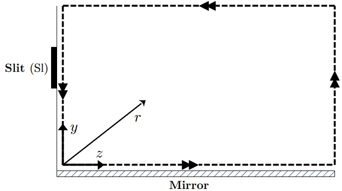
Figure 2: Surface integration for a Lloyd interferometer with corner geometry; the entrance slit is reaching from $(-\delta/2,0)$ to $(+\delta/2,0)$ in the $yz$-plane, and the double arrows follow the dotted closed integration path.

II.1.1 Exact solution

By the method of mirror charges, which is well-known from electrostatics [56], we obtain a Green’s function

$$G(\mathbf{r},\mathbf{r^{\prime}}) = \sum\limits_{a,b=\pm}ab\frac{e^{\mathrm{i}k\sqrt{(x-x^{\prime})^{2}+(y-ay^{\prime})^{2}+(z-bz^{\prime})^{2}}}}{\sqrt{(x-x^{\prime})^{2}+(y-ay^{\prime})^{2}+(z-bz^{\prime})^{2}}}\,\,\,,$$ (9)

which vanishes everywhere along the dotted integration path given in Fig. 2. We introduced $\mathbf{r}=(x,y,z)^{T}$ and $\mathbf{r}^{\prime}=(x^{\prime},y^{\prime},z^{\prime})^{T}$. In addition, the wave function $\psi(\mathbf{r^{\prime}})$ also vanishes everywhere on this path except for the part coinciding with the entrance slit. There we have $\psi(\mathbf{r^{\prime}})=Ce^{\mathrm{i}kz}$ with $C$ being some normalization constant. Using these properties together with the general solution in Eq. (8), we find

$$\psi(\mathbf{r}) = -\frac{1}{4\pi}\int_{\mathrm{Sl}}d\mathbf{S^{\prime}}\psi(\mathbf{r^{\prime}})\nabla^{\prime}G(\mathbf{r},\mathbf{r^{\prime}})$$ (10)

$$= \frac{1}{4\pi}\int_{-\infty}^{\infty}dx^{\prime}\int^{y_{\mathrm{Sl}}+\delta/2}_{y_{\mathrm{Sl}}-\delta/2}dy^{\prime}\psi(\mathbf{r^{\prime}})\frac{\partial}{\partial z^{\prime}}G(\mathbf{r},\mathbf{r^{\prime}})\,\,\,,$$

where $\mathrm{Sl}$ denotes the entrance slit area, and $y_{\mathrm{Sl}}$ and $\delta$ are the slit’s center and length on the $y$-coordinate. Substituting Eq. (9) into Eq. (10), we find

$$\psi(\mathbf{r}) = \frac{C}{2\pi}\frac{\partial}{\partial z}\int^{y_{\mathrm{Sl}}+\delta/2}_{y_{\mathrm{Sl}}-\delta/2}dy^{\prime}\int_{-\infty}^{\infty}dx^{\prime}\left[\frac{e^{\mathrm{i}k\sqrt{(x-x^{\prime})^{2}+(y+y^{\prime})^{2}+z^{2}}}}{\sqrt{(x-x^{\prime})^{2}+(y+y^{\prime})^{2}+z^{2}}}-\frac{e^{\mathrm{i}k\sqrt{(x-x^{\prime})^{2}+(y-y^{\prime})^{2}+z^{2}}}}{\sqrt{(x-x^{\prime})^{2}+(y-y^{\prime})^{2}+z^{2}}}\right]$$ (11)

$$= \frac{C}{2\pi}\frac{\partial}{\partial z}\int^{y_{\mathrm{Sl}}+\delta/2}_{y_{\mathrm{Sl}}-\delta/2}dy^{\prime}\int_{-\infty}^{\infty}dx\left[\frac{e^{\mathrm{i}k\sqrt{x^{2}+(y+y^{\prime})^{2}+z^{2}}}}{\sqrt{x^{2}+(y+y^{\prime})^{2}+z^{2}}}-\frac{e^{\mathrm{i}k\sqrt{x^{2}+(y-y^{\prime})^{2}+z^{2}}}}{\sqrt{x^{2}+(y-y^{\prime})^{2}+z^{2}}}\right]\,\,\,.$$

Next, we evaluate the $x$-integral via the following integral representation of the Hankel function of the first kind [56]:

$$\mathrm{i}\pi H_{0}^{(1)}(k\rho) = \int^{\infty}_{-\infty}dz\frac{e^{\mathrm{i}k\sqrt{\rho^{2}+z^{2}}}}{\sqrt{\rho^{2}+z^{2}}}\,\,\,.$$ (12)

In this way, we obtain

$$\psi(\mathbf{r}) = \frac{\mathrm{i}C}{2}\frac{\partial}{\partial z}\int^{y_{\mathrm{Sl}}+\delta/2}_{y_{\mathrm{Sl}}-\delta/2}dy^{\prime}\left[H_{0}^{(1)}(k\sqrt{(y+y^{\prime})^{2}+z^{2}})-H_{0}^{(1)}(k\sqrt{(y-y^{\prime})^{2}+z^{2}})\right]\,\,\,.$$ (13)

Next, using [57]

$$\frac{d}{dz}H_{n}^{(1)}(z) = \frac{nH_{n}^{(1)}(z)}{z}-H_{n+1}^{(1)}(z)\,\,\,,$$ (14)

we find

$$\psi(\mathbf{r}) = C\frac{\mathrm{i}kz}{2}\int^{y_{\mathrm{Sl}}+\delta/2}_{y_{\mathrm{Sl}}-\delta/2}dy^{\prime}\left[\frac{H_{1}^{(1)}(k\sqrt{(y-y^{\prime})^{2}+z^{2}})}{\sqrt{(y-y^{\prime})^{2}+z^{2}}}-\frac{H_{1}^{(1)}(k\sqrt{(y+y^{\prime})^{2}+z^{2}})}{\sqrt{(y+y^{\prime})^{2}+z^{2}}}\right]\,\,\,,$$ (15)

and ultimately

$$\psi(\mathbf{r}) = C\frac{\mathrm{i}kz}{2}\left[\int^{y_{\mathrm{Sl}}+\delta/2-y}_{y_{\mathrm{Sl}}-\delta/2-y}dy^{\prime}\frac{H_{1}^{(1)}(k\sqrt{y^{\prime 2}+z^{2}})}{\sqrt{y^{\prime 2}+z^{2}}}-\int^{y_{\mathrm{Sl}}+\delta/2+y}_{y_{\mathrm{Sl}}-\delta/2+y}dy^{\prime}\frac{H_{1}^{(1)}(k\sqrt{y^{\prime 2}+z^{2}})}{\sqrt{y^{\prime 2}+z^{2}}}\right]\,\,\,.$$ (16)

II.1.2 Asymptotic expression

We will now find an approximation for Eq. (16) by approximating its integrals in the asymptotic case that $z$ is very large and $\delta\to 0$. For this, we first use the asymptotic expression [56]

$$H_{1}^{(1)}(z) \to \sqrt{\frac{2}{\pi z}}e^{\mathrm{i}(z-3\pi/4)}\,\,\,,$$ (17)

which allows us to write Eq. (16) in the asymptotic case of $z$ being large as

$$\psi(\mathbf{r}) \to Cz\sqrt{\frac{k}{2\pi}}e^{-\mathrm{i}\pi/4}\left[\int^{y_{\mathrm{Sl}}+\delta/2-y}_{y_{\mathrm{Sl}}-\delta/2-y}dy^{\prime}\frac{e^{\mathrm{i}k\sqrt{y^{\prime 2}+z^{2}}}}{(y^{\prime 2}+z^{2})^{3/4}}-\int^{y_{\mathrm{Sl}}+\delta/2+y}_{y_{\mathrm{Sl}}-\delta/2+y}dy^{\prime}\frac{e^{\mathrm{i}k\sqrt{y^{\prime 2}+z^{2}}}}{(y^{\prime 2}+z^{2})^{3/4}}\right]\,\,\,.$$ (18)

Next, we use that for a convergent integrand and a small integration interval the following approximation holds:

$$\int^{A+\delta/2}_{A-\delta/2}dyf(y) = \int^{+\delta/2}_{-\delta/2}dyf(y+A)\,=\,\frac{\delta}{2}\int^{+1}_{-1}dyf\left(\frac{\delta}{2}y+A\right)\,\to\,\delta f(A)\,\,\,.$$ (19)

Applying this to Eq. (18), we find that the wave function for large $z$ and $\delta\to 0$ can be approximated as

$$\psi(\mathbf{r}) \to \delta Cz\sqrt{\frac{k}{2\pi}}e^{-\mathrm{i}\pi/4}\left\{\frac{e^{\mathrm{i}k\sqrt{(y_{\mathrm{Sl}}-y)^{2}+z^{2}}}}{[(y_{\mathrm{Sl}}-y)^{2}+z^{2}]^{3/4}}-\frac{e^{\mathrm{i}k\sqrt{(y_{\mathrm{Sl}}+y)^{2}+z^{2}}}}{[(y_{\mathrm{Sl}}+y)^{2}+z^{2}]^{3/4}}\right\}\,\,\,.$$ (20)

II.2 Gravitational field

Now we will consider a physically realistic situation by introducing an external gravitational field. At first, we will derive a general expression for the Green’s function for this particular case, following the treatment in Ref. [56]. Later, we will apply the result explicitly to Lloyd interferometry.

II.2.1 General solution

We consider a gravitational field in $x$-direction and want to find the Green’s function for the Helmholtz equation

$$\mathfrak{L}\psi(\mathbf{r}) = 0\,\,\,,$$ (21)

where the field operator is given by

$$\mathfrak{L} := \Delta_{\perp}+\partial_{x}^{2}+\frac{2m}{\hbar^{2}}(E-mgx)\,\,\,,$$ (22)

and we use the ansatz

$$G(\mathbf{r},\mathbf{r^{\prime}}) = 4\pi\int\frac{d^{2}k_{\perp}}{(2\pi)^{2}}e^{\mathrm{i}\mathbf{k}_{\perp}\cdot(\mathbf{x}_{\perp}-\mathbf{x^{\prime}}_{\perp})}\mathrm{g}(x,x^{\prime};\mathbf{k}_{\perp})$$ (23)

for the Green’s function. Consequently, acting with the field operator from Eq. (22) on the Green’s function gives us the following condition:

$$\mathfrak{L}G(\mathbf{r},\mathbf{r^{\prime}}) = 4\pi\int\frac{d^{2}k_{\perp}}{(2\pi)^{2}}e^{\mathrm{i}\mathbf{k}_{\perp}\cdot(\mathbf{x}_{\perp}-\mathbf{x^{\prime}}_{\perp})}\left[\partial_{x}^{2}-\mathbf{k}_{\perp}^{2}+\frac{2m}{\hbar^{2}}(E-mgx)\right]\mathrm{g}(x,x^{\prime};\mathbf{k}_{\perp})$$ (24)

$$= 4\pi\int\frac{d^{2}k_{\perp}}{(2\pi)^{2}}e^{\mathrm{i}\mathbf{k}_{\perp}\cdot(\mathbf{x}_{\perp}-\mathbf{x^{\prime}}_{\perp})}\left[\partial_{x}^{2}+\frac{2m}{\hbar^{2}}(\tilde{E}-mgx)\right]\mathrm{g}(x,x^{\prime};\mathbf{k}_{\perp})$$

$$= -4\pi\delta^{(3)}(\mathbf{r}-\mathbf{r^{\prime}})$$

with $\tilde{E}:=E-\hbar^{2}\mathbf{k}_{\perp}^{2}/2m$. Subsequently, we extract

$$\left[\partial_{x}^{2}+\frac{2m}{\hbar^{2}}(\tilde{E}-mgx)\right]\mathrm{g}(x,x^{\prime};\mathbf{k}_{\perp}) = -\delta(x-x^{\prime})\,\,\,.$$ (25)

Assuming that $\mathrm{g}$ has support only on $\{x\!:x\in[x^{\prime}-0,x^{\prime}+0]\}$, integrating Eq. (25) over $x$ gives

$$\left.\partial_{x}\mathrm{g}(x,x^{\prime};\mathbf{k}_{\perp})\right|^{x^{\prime}+0}_{x^{\prime}-0} = -1\,\,\,.$$ (26)

Next, we return to Eq. (25) and multiply it with $x$ from the left, which leads us to

$$\partial_{x}\left[x\partial_{x}\mathrm{g}(x,x^{\prime};\mathbf{k}_{\perp})-\mathrm{g}(x,x^{\prime};\mathbf{k}_{\perp})\right]+\frac{2mx}{\hbar^{2}}(\tilde{E}-mgx)\mathrm{g}(x,x^{\prime};\mathbf{k}_{\perp}) = -x^{\prime}\delta(x-x^{\prime})\,\,\,.$$ (27)

Integrating this over $x$, we find

$$\left.x\partial_{x}\mathrm{g}(x,x^{\prime};\mathbf{k}_{\perp})\right|^{x^{\prime}+0}_{x^{\prime}-0}-\left.\mathrm{g}(x,x^{\prime};\mathbf{k}_{\perp})\right|^{x^{\prime}+0}_{x^{\prime}-0} = -x^{\prime}\,\,\,.$$ (28)

Combining Eqs. (26) and (28), gives

$$\left.\mathrm{g}(x,x^{\prime};\mathbf{k}_{\perp})\right|^{x^{\prime}+0}_{x^{\prime}-0} = 0\,\,\,.$$ (29)

For later convenience, we are now going to prove the reciprocity relation

$$\mathrm{g}(x,x^{\prime};\mathbf{k}_{\perp}) = \mathrm{g}(x^{\prime},x;\mathbf{k}_{\perp})\,\,\,.$$ (30)

For this, we begin by multiplying Eq. (25) by $\mathrm{g}(x,x^{\prime\prime};\mathbf{k}_{\perp})$, and then subtracting a copy of the resulting equation but with $x^{\prime}\leftrightarrow x^{\prime\prime}$, which results in

$$-\mathrm{g}(x,x^{\prime\prime};\mathbf{k}_{\perp})\delta(x-x^{\prime})+\mathrm{g}(x,x^{\prime};\mathbf{k}_{\perp})\delta(x-x^{\prime\prime}) = \mathrm{g}(x,x^{\prime\prime};\mathbf{k}_{\perp})\partial_{x}^{2}\mathrm{g}(x,x^{\prime};\mathbf{k}_{\perp})$$ (31)

$$\,\,\,\,\,\,\,\,\,\,\,\,\,\,\,\,\,\,\,\,\,\,\,\,\,\,\,\,\,\,\,\,-\mathrm{g}(x,x^{\prime};\mathbf{k}_{\perp})\partial_{x}^{2}\mathrm{g}(x,x^{\prime\prime};\mathbf{k}_{\perp})$$

$$= \partial_{x}\left[\mathrm{g}(x,x^{\prime\prime};\mathbf{k}_{\perp})\partial_{x}\mathrm{g}(x,x^{\prime};\mathbf{k}_{\perp})\right.$$

$$\,\,\,\,\,\,\,\,\,\,\,\,\,\,\,\,\,\,\,\,\,\,\,\,\,\,\,\,\,\,\,\,\,\,\,\,\,\,\,\,\,\left.-\mathrm{g}(x,x^{\prime};\mathbf{k}_{\perp})\partial_{x}\mathrm{g}(x,x^{\prime\prime};\mathbf{k}_{\perp})\right]\,\,\,.\,\,\,\,\,\,\,\,\,\,\,\,\,\,\,\,\,\,$$

Integrating this over all of $x$ yields

$$-\mathrm{g}(x^{\prime},x^{\prime\prime};\mathbf{k}_{\perp})+\mathrm{g}(x^{\prime\prime},x^{\prime};\mathbf{k}_{\perp}) = \left[\mathrm{g}(x,x^{\prime\prime};\mathbf{k}_{\perp})\partial_{x}\mathrm{g}(x,x^{\prime};\mathbf{k}_{\perp})-\mathrm{g}(x,x^{\prime};\mathbf{k}_{\perp})\partial_{x}\mathrm{g}(x,x^{\prime\prime};\mathbf{k}_{\perp})\right]|^{+\infty}_{-\infty}\,\,\,.\,\,\,\,\,\,\,\,\,\,\,$$ (32)

Since $\mathrm{g}$ has support only on $\{x\!:x\in[x^{\prime}-0,x^{\prime}+0]\}$, we know that the right-hand side of Eq. (32) must vanish, leaving us with the reciprocity relation

$$\mathrm{g}(x^{\prime},x^{\prime\prime};\mathbf{k}_{\perp}) = \mathrm{g}(x^{\prime\prime},x^{\prime};\mathbf{k}_{\perp})\,\,\,,$$ (33)

which concludes the proof.
Now we continue with the computation of the function $\mathrm{g}(x,x^{\prime};\mathbf{k}_{\perp})$. For this, we use that for $x\neq x^{\prime}$ Eq. (25) takes on the form

$$\left[\partial_{x}^{2}+\frac{2m}{\hbar^{2}}(\tilde{E}-mgx)\right]\mathrm{g}(x,x^{\prime};\mathbf{k}_{\perp}) = 0\,\,\,.$$ (34)

In this way, we can find a solution for the Green’s function via the homogeneous solution. Following Ref. [39], the convergent solution of Eq. (34) for $x\geq x^{\prime}$ is

$$\mathrm{g}(x,x^{\prime};\mathbf{k}_{\perp}) = C_{1}(x^{\prime})\mathrm{Ai}(\sigma)$$ (35)

with a dimensionless variable

$$\sigma := \sqrt[3]{\frac{2m^{2}g}{\hbar^{2}}}\left(x-\frac{\tilde{E}}{mg}\right)\,\,\,,$$ (36)

while for $x\leq x^{\prime}$ it is

$$\mathrm{g}(x,x^{\prime};\mathbf{k}_{\perp}) = C_{2}(x^{\prime})\mathrm{Ai}(\sigma)+C_{3}(x^{\prime})\mathrm{Bi}(\sigma)\,\,\,.$$ (37)

$\mathrm{Ai}$ and $\mathrm{Bi}$ are Airy functions of the first and second kind, respectively. Applying the conditions in Eqs. (26) and (29) to the solutions in Eqs. (35) and (37) leads us to

$$C_{1}(x^{\prime})\mathrm{Ai}^{\prime}(\sigma^{\prime})-C_{2}(x^{\prime})\mathrm{Ai}^{\prime}(\sigma^{\prime})-C_{3}(x^{\prime})\mathrm{Bi}^{\prime}(\sigma^{\prime})\,=\,-\sqrt[3]{\frac{\hbar^{2}}{2m^{2}g}}\,\,\,,$$ (38)

$$C_{1}(x^{\prime})\mathrm{Ai}(\sigma^{\prime})\,-\,C_{2}(x^{\prime})\mathrm{Ai}(\sigma^{\prime})\,-\,C_{3}(x^{\prime})\mathrm{Bi}(\sigma^{\prime})\,\,=\,0\,\,\,,$$ (39)

where

$$\sigma^{\prime} := \sqrt[3]{\frac{2m^{2}g}{\hbar^{2}}}\left(x^{\prime}-\frac{\tilde{E}}{mg}\right)\,\,\,.$$ (40)

Combining Eqs. (38) and (39) gives

$$C_{1}(x^{\prime}) = C_{2}(x^{\prime})+\sqrt[3]{\frac{\hbar^{2}}{2m^{2}g}}\frac{\mathrm{Bi}(\sigma^{\prime})}{W(\mathrm{Ai},\mathrm{Bi})(\sigma^{\prime})}\,\,\,,\,\,\,\,\,\,\,\,\,C_{3}(x^{\prime})\,=\,\sqrt[3]{\frac{\hbar^{2}}{2m^{2}g}}\frac{\mathrm{Ai}(\sigma^{\prime})}{W(\mathrm{Ai},\mathrm{Bi})(\sigma^{\prime})}\,\,\,,$$ (41)

where $W(\mathrm{Ai},\mathrm{Bi})(\sigma)$ is the Wronskian of $\mathrm{Ai}$ and $\mathrm{Bi}$. Using the fact that every Airy function $f(\sigma)$ must fulfill $f^{\prime\prime}(\sigma)=\sigma f(\sigma)$, it is straightforward to show that this Wronskian must be constant:

$$\frac{d}{d\sigma}W(\mathrm{Ai},\mathrm{Bi})(\sigma) = \mathrm{Ai}(\sigma)\mathrm{Bi}^{\prime\prime}(\sigma)-\mathrm{Bi}(\sigma)\mathrm{Ai}^{\prime\prime}(\sigma)$$ (42)

$$= \sigma\mathrm{Ai}(\sigma)\mathrm{Bi}(\sigma)-\sigma\mathrm{Bi}(\sigma)\mathrm{Ai}(\sigma)$$

$$= 0\,\,\,,$$

which implies $W(\mathrm{Ai},\mathrm{Bi})(\sigma)=W(\mathrm{Ai},\mathrm{Bi})(0)$. Taking the values for the Airy functions and their derivatives at $\sigma=0$, we can show that

$$W(\mathrm{Ai},\mathrm{Bi})(\sigma) = \frac{1}{\pi}$$ (43)

holds. So, substituting this into Eqs. (35) and (37) leaves us with

$$\mathrm{g}(x,x^{\prime};\mathbf{k}_{\perp}) = 2C_{2}(x^{\prime})\mathrm{Ai}(\sigma)+\sqrt[3]{\frac{\hbar^{2}\pi^{3}}{2m^{2}g}}\left[\Theta(x-x^{\prime})\mathrm{Bi}(\sigma^{\prime})\mathrm{Ai}(\sigma)+\Theta(x^{\prime}-x)\mathrm{Ai}(\sigma^{\prime})\mathrm{Bi}(\sigma)\right]\,\,\,.\,\,\,\,\,\,\,\,\,\,\,\,$$ (44)

Furthermore, from the reciprocity relation (30) we conclude

$$C_{2}(x^{\prime}) = \frac{\lambda}{2}\mathrm{Ai}(\sigma^{\prime})\,\,\,,$$ (45)

where $\lambda$ is some constant. In consequence, we have

$$\mathrm{g}(x,x^{\prime};\mathbf{k}_{\perp}) = \lambda\mathrm{Ai}(\sigma)\mathrm{Ai}(\sigma^{\prime})+\sqrt[3]{\frac{\hbar^{2}\pi^{3}}{2m^{2}g}}\left[\Theta(x-x^{\prime})\mathrm{Ai}(\sigma)\mathrm{Bi}(\sigma^{\prime})+\Theta(x^{\prime}-x)\mathrm{Ai}(\sigma^{\prime})\mathrm{Bi}(\sigma)\right]\,\,\,.\,\,\,\,\,\,\,\,\,\,\,\,$$ (46)

Substituting Eq. (46) into the ansatz in Eq. (23), we obtain the solution for the Green’s function as

$$G(\mathbf{r},\mathbf{r^{\prime}}) = 4\pi\int\frac{d^{2}k_{\perp}}{(2\pi)^{2}}e^{\mathrm{i}\mathbf{k}_{\perp}\cdot(\mathbf{x}_{\perp}-\mathbf{x^{\prime}}_{\perp})}$$ (47)

$$\times\left\{\lambda\mathrm{Ai}(\sigma)\mathrm{Ai}(\sigma^{\prime})+\sqrt[3]{\frac{\hbar^{2}\pi^{3}}{2m^{2}g}}[\Theta(x-x^{\prime})\mathrm{Ai}(\sigma)\mathrm{Bi}(\sigma^{\prime})+\Theta(x^{\prime}-x)\mathrm{Ai}(\sigma^{\prime})\mathrm{Bi}(\sigma)]\right\}\,\,\,.\,\,\,\,\,\,\,\,\,\,\,\,$$

II.2.2 Lloyd interferometer

We can now take this general result and apply it to the situation in a Lloyd interferometer. For this, we again use the method of mirror charges in order to determine the Green’s function:

$$G(\mathbf{r},\mathbf{r^{\prime}}) = 4\pi\int\frac{d^{2}k_{\perp}}{(2\pi)^{2}}\sum\limits_{a,b=\pm}ab\,e^{\mathrm{i}k_{y}(y-ay^{\prime})+\mathrm{i}k_{z}(z-bz^{\prime})}$$ (48)

$$\times\left\{\lambda\mathrm{Ai}(\sigma)\mathrm{Ai}(\sigma^{\prime})+\sqrt[3]{\frac{\hbar^{2}\pi^{3}}{2m^{2}g}}[\Theta(x-x^{\prime})\mathrm{Ai}(\sigma)\mathrm{Bi}(\sigma^{\prime})+\Theta(x^{\prime}-x)\mathrm{Ai}(\sigma^{\prime})\mathrm{Bi}(\sigma)]\right\}\,\,\,.\,\,\,\,\,\,\,\,\,\,\,\,$$

Again this Green’s function vanishes along the dotted integration path depicted in Fig. 2, and the wave function $\psi(\mathbf{r})$ is only non-vanishing and equals $Ce^{\mathrm{i}kz}$ at the entrance slit. Eq. (10) still holds. Substituting Eq. (48) into Eq. (10) and taking the $z^{\prime}$-derivative, we find

$$\psi(\mathbf{r}) = -4C\int_{-\infty}^{\infty}dx^{\prime}\int^{y_{\mathrm{Sl}}+\delta/2}_{y_{\mathrm{Sl}}-\delta/2}dy^{\prime}\int\frac{d^{2}k_{\perp}}{(2\pi)^{2}}k_{z}\sin(k_{y}y^{\prime})e^{\mathrm{i}\mathbf{k}_{\perp}\cdot\mathbf{x}_{\perp}}$$ (49)

$$\times\left\{\lambda\mathrm{Ai}(\sigma)\mathrm{Ai}(\sigma^{\prime})+\sqrt[3]{\frac{\hbar^{2}\pi^{3}}{2m^{2}g}}[\Theta(x-x^{\prime})\mathrm{Ai}(\sigma)\mathrm{Bi}(\sigma^{\prime})+\Theta(x^{\prime}-x)\mathrm{Ai}(\sigma^{\prime})\mathrm{Bi}(\sigma)]\right\}\,\,\,.\,\,\,\,\,\,\,\,\,\,\,\,$$

Also evaluating the $y^{\prime}$-integral and redefining the constant $\sqrt[3]{\frac{2m^{2}g}{\hbar^{2}}}\lambda\to\lambda$, we are left with

$$\psi(\mathbf{r}) = -8C\int\frac{d^{2}k_{\perp}}{(2\pi)^{2}}\frac{k_{z}}{k_{y}}\sin(k_{y}y_{\mathrm{Sl}})\sin(k_{y}\delta/2)e^{\mathrm{i}\mathbf{k}_{\perp}\cdot\mathbf{x}_{\perp}}$$ (50)

$$\times\int_{-\infty}^{\infty}d\sigma^{\prime}\left\{\lambda\mathrm{Ai}(\sigma)\mathrm{Ai}(\sigma^{\prime})+\pi[\Theta(\sigma-\sigma^{\prime})\mathrm{Ai}(\sigma)\mathrm{Bi}(\sigma^{\prime})+\Theta(\sigma^{\prime}-\sigma)\mathrm{Ai}(\sigma^{\prime})\mathrm{Bi}(\sigma)]\right\}\,\,\,.\,\,\,\,\,\,\,\,\,\,\,\,$$

Since [58]

$$\int_{-\infty}^{\infty}d\sigma^{\prime}\mathrm{Ai}(\sigma^{\prime}) = 1\,\,\,,$$ (51)

and

$$\!\!\!\!\!\!\!\!\!\!\!\!\!\!\!\!\int_{-\infty}^{\infty}d\sigma^{\prime}[\Theta(\sigma-\sigma^{\prime})\mathrm{Ai}(\sigma)\mathrm{Bi}(\sigma^{\prime})+\Theta(\sigma^{\prime}-\sigma)\mathrm{Ai}(\sigma^{\prime})\mathrm{Bi}(\sigma)]$$

$$=\frac{1}{3}\mathrm{Bi}(\sigma)+\frac{\sigma^{2}}{2\pi}\left[{}_{0}F_{1}\bigg{(};\frac{2}{3};\frac{\sigma^{3}}{9}\bigg{)}{}_{1}F_{2}\bigg{(}\frac{2}{3};\frac{4}{3},\frac{5}{3};\frac{\sigma^{3}}{9}\bigg{)}-2{}_{0}F_{1}\bigg{(};\frac{4}{3};\frac{\sigma^{3}}{9}\bigg{)}{}_{1}F_{2}\bigg{(}\frac{1}{3};\frac{2}{3},\frac{4}{3};\frac{\sigma^{3}}{9}\bigg{)}\right]\,\,\,,$$ (52)

we finally obtain

$$\psi(\mathbf{r}) = -8C\int\frac{d^{2}k_{\perp}}{(2\pi)^{2}}\frac{k_{z}}{k_{y}}\sin(k_{y}y_{\mathrm{Sl}})\sin(k_{y}\delta/2)e^{\mathrm{i}\mathbf{k}_{\perp}\cdot\mathbf{x}_{\perp}}$$ (53)

$$\times\left\{\lambda\mathrm{Ai}(\sigma)+\frac{\pi}{3}\mathrm{Bi}(\sigma)+\frac{\sigma^{2}}{2}\bigg{[}{}_{0}F_{1}\bigg{(};\frac{2}{3};\frac{\sigma^{3}}{9}\bigg{)}{}_{1}F_{2}\bigg{(}\frac{2}{3};\frac{4}{3},\frac{5}{3};\frac{\sigma^{3}}{9}\bigg{)}\right.$$

$$\phantom{\times\left\{\lambda\mathrm{Ai}(\sigma)+\frac{\pi}{3}\mathrm{Bi}(\sigma)+[\right.}\,\,\,\,\,\left.-2{}_{0}F_{1}\bigg{(};\frac{4}{3};\frac{\sigma^{3}}{9}\bigg{)}{}_{1}F_{2}\bigg{(}\frac{1}{3};\frac{2}{3},\frac{4}{3};\frac{\sigma^{3}}{9}\bigg{)}\bigg{]}\right\}\,\,\,.\,\,\,\,\,\,\,\,\,\,\,\,$$

III Conclusions

Neutron Lloyd interferometry is a promising experimental setup that can be used to probe effects within and beyond the realms of known physics. However, previous theoretical analyses made use of approximative methods, which are expected to not always be sufficiently accurate. For this reason, in this article, we presented an exact full Green’s functions analysis of Lloyd interferometry. First, we discussed the hypothetical case of no external fields acting on the neutrons while travelling within the experimental setup. For this, we found the corresponding Green’s function for solving the Schrödinger equation and subsequently determined the resulting wave function. Second, we looked at the physically relevant case of having an external gravitational field acting on the neutrons.
The prediction made for the gravitationally modified neutron wave function serves as a theoretical basis for using a neutron Lloyd interferometer to probe gravitational fields. However, it should be stressed that the computations presented here approximate the interferometer’s slit source as being infinitely wide in $x$-direction and the mirror to be infinitely extended. For practically applying the technology developed in this article to a real experiment, a numerical analysis without these approximations would be required. Such a sophisticated numerical evaluation will be subject of future work. Furthermore, in the future, the computation shown in the present article, will serve as a blueprint for predicting neutron wave functions in Lloyd interferometers under the influence of hypothetical gravity-like fifth forces and scalar fields.

References

• [1] H. Lloyd, On a New Case of Interference of the Rays of Light, in The Transactions of the Royal Irish Academy, vol. 17, p. 171–177. 1831.
• [2] P. H. Langenbeck, Lloyd Interferometer Applied to Flatness Testing, Appl. Opt. 6 (1967) 1707.
• [3] P. Langenbeck, Higher-Order Lloyd Interferometer, Appl. Opt. 9 (1970) 1838.
• [4] L. S. Watkins and A. Tvarusko, Lloyd Mirror Laser Interferometer for Diffusion Layer Studies, Review of Scientific Instruments 41 (1970) 1860 [https://doi.org/10.1063/1.1684430].
• [5] J. Kielkopf and L. Portaro, Lloyd’s mirror as a laser wavemeter, Appl. Opt. 31 (1992) 7083.
• [6] J. J. Rocca, C. H. Moreno, M. C. Marconi and K. Kanizay, Soft-x-ray laser interferometry of a plasma with a tabletop laser and a Lloyd’s mirror, Opt. Lett. 24 (1999) 420.
• [7] S. R. Abdullina, A. A. Vlasov and S. A. Babin, Smoothing of the spectrum of fibre Bragg gratings in the Lloyd-interferometer recording scheme, Quantum Electronics 40 (2010) 259.
• [8] I. Wathuthanthri, W. Mao and C.-H. Choi, Two degrees-of-freedom Lloyd–mirror interferometer for superior pattern coverage area, Opt. Lett. 36 (2011) 1593.
• [9] X. Li, Y. Shimizu, S. Ito, W. Gao and L. Zeng, Fabrication of diffraction gratings for surface encoders by using a Lloyd’s mirror interferometer with a 405 nm laser diode, in Eighth International Symposium on Precision Engineering Measurement and Instrumentation (J. Lin, ed.), vol. 8759, p. 87594Q, International Society for Optics and Photonics, SPIE, 2013, DOI.
• [10] Z. Ren, R. Aihara, Y. Shimizu, S. Ito, Y.-L. Chen and W. Gao, Analysis of a Lloyd’s mirror interferometer for fabrication of gratings, in 2016 IEEE 16th International Conference on Nanotechnology (IEEE-NANO), pp. 982–983, 2016, DOI.
• [11] X. Li, H. Lu, Q. Zhou, G. Wu, K. Ni and X. Wang, An Orthogonal Type Two-Axis Lloyd’s Mirror for Holographic Fabrication of Two-Dimensional Planar Scale Gratings with Large Area, Applied Sciences 8 (2018) .
• [12] M. Rani, A. Shankar and R. Kumar, Effect of quality of opto-mechanical components on fringes of diffraction Lloyd mirror interferometer, Results in Optics 8 (2022) 100265.
• [13] V. P. Gudkov, G. I. Opat and A. G. Klein, Neutron reflection interferometry: physical principles of surface analysis with phase information, Journal of Physics: Condensed Matter 5 (1993) 9013.
• [14] Y. N. Pokotilovski, Neutron experiments to search for new spin-dependent interactions, JETP Lett. 94 (2011) 413 [1107.1481].
• [15] H. M. Filter, Interference experiment with slow neutrons: a feasibility study of Lloyd’s mirror at the Institut Laue-Langevin, Ph.D. thesis, Technische Universität Wien, reposiTUm. https://doi.org/10.34726/hss.2018.37910, 2018.
• [16] H. Rauch, W. Treimer and U. Bonse, Test of a single crystal neutron interferometer, Physics Letters A 47 (1974) 369.
• [17] H. Rauch and S. Werner, Neutron Interferometry: Lessons in Experimental Quantum Mechanics, Wave-Particle Duality, and Entanglement. OUP Oxford, 2015.
• [18] H. Abele, The neutron. Its properties and basic interactions, Prog. Part. Nucl. Phys. 60 (2008) 1.
• [19] D. Dubbers and M. G. Schmidt, The Neutron and Its Role in Cosmology and Particle Physics, Rev. Mod. Phys. 83 (2011) 1111 [1105.3694].
• [20] W. Mampe, P. Ageron, C. Bates, J. Pendlebury and A. Steyerl, Neutron lifetime measured with stored ultracold neutrons, Physical Review Letters 63 (1989) 593.
• [21] S. Arzumanov, L. Bondarenko, S. Chernavsky, A. Fomin, V. Morozov, Y. Panin et al., Neutron life time value measured by storing ultracold neutrons with detection of inelastically scattered neutrons, Phys. Lett. B 483 (2000) 15.
• [22] A. P. Serebrov et al., Neutron lifetime measurements using gravitationally trapped ultracold neutrons, Phys. Rev. C 78 (2008) 035505 [nucl-ex/0702009].
• [23] V. Ezhov, A. Andreev, G. Ban, B. Bazarov, P. Geltenbort, F. Hartman et al., Magnetic storage of ucn for a measurement of the neutron lifetime, Nuclear Instruments and Methods in Physics Research Section A: Accelerators, Spectrometers, Detectors and Associated Equipment 611 (2009) 167.
• [24] A. Pichlmaier, V. Varlamov, K. Schreckenbach and P. Geltenbort, Neutron lifetime measurement with the UCN trap-in-trap MAMBO II, Phys. Lett. B 693 (2010) 221.
• [25] A. P. Serebrov et al., Neutron lifetime measurements with a large gravitational trap for ultracold neutrons, Phys. Rev. C 97 (2018) 055503 [1712.05663].
• [26] R. W. Pattie, Jr. et al., Measurement of the neutron lifetime using a magneto-gravitational trap and in situ detection, Science 360 (2018) 627 [1707.01817].
• [27] V. F. Ezhov et al., Measurement of the neutron lifetime with ultra-cold neutrons stored in a magneto-gravitational trap, JETP Lett. 107 (2018) 671 [1412.7434].
• [28] UCNA collaboration, R. W. Pattie et al., First Measurement of the Neutron beta-Asymmetry with Ultracold Neutrons, Phys. Rev. Lett. 102 (2009) 012301 [0809.2941].
• [29] UCNA collaboration, M. P. Mendenhall et al., Precision measurement of the neutron $\beta$-decay asymmetry, Phys. Rev. C 87 (2013) 032501 [1210.7048].
• [30] UCNA collaboration, M. A. P. Brown et al., New result for the neutron $\beta$-asymmetry parameter $A_{0}$ from UCNA, Phys. Rev. C 97 (2018) 035505 [1712.00884].
• [31] V. I. Luschikov and A. I. Frank, Quantum effects occurring when ultracold neutrons are stored on a plane, JETP Lett. (USSR) (Engl. Transl.); (United States) 28:9 (1978) .
• [32] H. Rauch and S. A. Werner, Neutron Interferometry: Lessons in Experimental Quantum Mechanics, Wave-Particle Duality, and Entanglement, vol. 12. Oxford University Press, USA, 2015.
• [33] A. I. i. Frank, P. Geltenbort, G. Kulin, D. Kustov, V. Nosov and A. N. Strepetov, Effect of accelerating matter in neutron optics, JETP letters 84 (2006) 363.
• [34] A. I. i. Frank, P. Geltenbort, M. Jentschel, D. Kustov, G. Kulin and A. N. Strepetov, New experiment on the observation of the effect of accelerating matter in neutron optics, JETP letters 93 (2011) 361.
• [35] K. Durstberger-Rennhofer, T. Jenke and H. Abele, Probing neutron’s electric neutrality with Ramsey Spectroscopy of gravitational quantum states of ultra-cold neutrons, Phys. Rev. D 84 (2011) 036004 [1105.6180].
• [36] C. Abel et al., Measurement of the Permanent Electric Dipole Moment of the Neutron, Phys. Rev. Lett. 124 (2020) 081803 [2001.11966].
• [37] H. Abele, A. Ivanov, T. Jenke, M. Pitschmann and P. Geltenbort, Gravity Resonance Spectroscopy and Einstein-Cartan Gravity, in 11th Patras Workshop on Axions, WIMPs and WISPs, pp. 124–129, 2015, 1510.03063, DOI.
• [38] T. Jenke et al., Testing gravity at short distances: Gravity Resonance Spectroscopy with $q$BOUNCE, EPJ Web Conf. 219 (2019) 05003.
• [39] M. Pitschmann and H. Abele, Schrödinger Equation for a Non-Relativistic Particle in a Gravitational Field confined by Two Vibrating Mirrors, 1912.12236.
• [40] R. I. P. Sedmik et al., Proof of Principle for Ramsey-type Gravity Resonance Spectroscopy with qBounce, EPJ Web Conf. 219 (2019) 05004 [1908.09723].
• [41] T. Jenke, J. Bosina, J. Micko, M. Pitschmann, R. Sedmik and H. Abele, Gravity resonance spectroscopy and dark energy symmetron fields: qBOUNCE experiments performed with Rabi and Ramsey spectroscopy, Eur. Phys. J. ST 230 (2021) 1131 [2012.07472].
• [42] M. Suda, M. Faber, J. Bosina, T. Jenke, C. Käding, J. Micko et al., Spectra of Neutron Wave Functions in Earth’s Gravitational Field, Zeitschrift für Naturforschung A 77 (2022) 875 [2111.02769].
• [43] A. N. Ivanov, M. Wellenzohn and H. Abele, Quantum gravitational states of ultracold neutrons as a tool for probing of beyond-Riemann gravity, Phys. Lett. B 822 (2021) 136640 [2109.09982].
• [44] N. Muto et al., A novel nuclear emulsion detector for measurement of quantum states of ultracold neutrons in the Earth’s gravitational field, JINST 17 (2022) P07014 [2201.04346].
• [45] H. Lemmel, P. Brax, A. N. Ivanov, T. Jenke, G. Pignol, M. Pitschmann et al., Neutron Interferometry constrains dark energy chameleon fields, Phys. Lett. B 743 (2015) 310 [1502.06023].
• [46] A. N. Ivanov, G. Cronenberg, R. Höllwieser, M. Pitschmann, T. Jenke, M. Wellenzohn et al., Exact solution for chameleon field, self-coupled through the Ratra-Peebles potential with $n=1$ and confined between two parallel plates, Phys. Rev. D 94 (2016) 085005 [1606.06867].
• [47] P. Brax and M. Pitschmann, Exact solutions to nonlinear symmetron theory: One- and two-mirror systems, Phys. Rev. D 97 (2018) 064015 [1712.09852].
• [48] G. Cronenberg, P. Brax, H. Filter, P. Geltenbort, T. Jenke, G. Pignol et al., Acoustic Rabi oscillations between gravitational quantum states and impact on symmetron dark energy, Nature Phys. 14 (2018) 1022 [1902.08775].
• [49] A. N. Ivanov, M. Wellenzohn and H. Abele, Probing of violation of Lorentz invariance by ultracold neutrons in the Standard Model Extension, Phys. Lett. B 797 (2019) 134819 [1908.01498].
• [50] M. Pitschmann, Exact solutions to nonlinear symmetron theory: One- and two-mirror systems. II., Phys. Rev. D 103 (2021) 084013 [2012.12752].
• [51] S. Sponar, R. I. P. Sedmik, M. Pitschmann, H. Abele and Y. Hasegawa, Tests of fundamental quantum mechanics and dark interactions with low-energy neutrons, Nature Rev. Phys. 3 (2021) 309 [2012.09048].
• [52] P. Brax, H. Fischer, C. Käding and M. Pitschmann, The environment dependent dilaton in the laboratory and the solar system, Eur. Phys. J. C 82 (2022) 934 [2203.12512].
• [53] Y. N. Pokotilovski, Strongly coupled chameleon fields: Possible test with a neutron Lloyd’s mirror interferometer, Phys. Lett. B 719 (2013) 341 [1203.5017].
• [54] Y. N. Pokotilovski, Potential of the neutron Lloyd‘s mirror interferometer for the search for new interactions, J. Exp. Theor. Phys. 116 (2013) 609 [1311.4679].
• [55] Č. Brukner and A. Zeilinger, Diffraction of matter waves in space and in time, Phys. Rev. A 56 (1997) 3804.
• [56] J. Schwinger, L. L. DeRaad Jr., K. A. Milton and W.-Y. Tsai, Classical Electrodynamics. Perseus Books, 1998.
• [57] G. N. Watson, A Treatise on the Theory of Bessel Functions. Cambridge University Press, 1966.
• [58] F. Olver, D. Lozier, R. Boisvert and C. Clark, The NIST Handbook of Mathematical Functions. Cambridge University Press, New York, NY, 2010-05-12, 2010.