Aligned Diffusion Schrödinger Bridges

Abstract

Diffusion Schrödinger bridges (DSB) have recently emerged as a powerful framework for recovering stochastic dynamics via their marginal observations at different time points. Despite numerous successful applications, existing algorithms for solving diffusion Schrödinger bridges have so far failed to utilize the structure of aligned data, which naturally arises in many biological phenomena. In this paper, we propose a novel algorithmic framework that, for the first time, solves DSBs while respecting the data alignment. Our approach hinges on a combination of two decades-old ideas: The classical Schrödinger bridge theory and Doob’s $h$-transform. Compared to prior methods, our approach leads to a simpler training procedure with lower variance, which we further augment with principled regularization schemes. This ultimately leads to sizeable improvements across experiments on synthetic and real data, including the tasks of predicting conformational changes in proteins and temporal evolution of cellular differentiation processes.

1 Introduction

The task of transforming a given distribution into another lies at the heart of many modern machine learning applications such as single-cell genomics (Tong et al., 2020; Schiebinger et al., 2019; Bunne et al., 2022a), meteorology (Fisher et al., 2009), and robotics (Chen et al., 2021a). To this end, diffusion Schrödinger bridges (De Bortoli et al., 2021; Chen et al., 2022a; Vargas et al., 2021; Liu et al., 2022b) have recently emerged as a powerful paradigm due to their ability to generalize prior deep diffusion-based models, notably score matching with Langevin dynamics (Song and Ermon, 2019; Song et al., 2021) and denoising diffusion probabilistic models (Ho et al., 2020), which have achieved the state-of-the-art on many generative modeling problems.

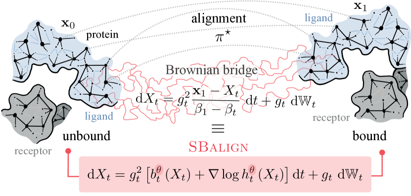
Figure 1: Overview of SBalign: In biological tasks such as protein docking, one is naturally provided with aligned data in the form of unbound and bound structures of participating proteins. Our goal is to therefore recover a stochastic trajectory from the unbound ($\mathbf{x}_{0}$) to the bound ($\mathbf{x}_{1}$) structure. To achieve this, we connect the characterization of an SDE conditioned on $\mathbf{x}_{0}$ and $\mathbf{x}_{1}$ (utilizing the Doob’s $h$-transform) with that of a Brownian bridge between $\mathbf{x}_{0}$ and $\mathbf{x}_{1}$ (classical Schrödinger bridge theory). We show that this leads to a simpler training procedure with lower variance and strong empirical results.

Despite the wide success of DSBs solvers, a significant limitation of existing frameworks is that they fail to capture the alignment of data: If $\hat{\mathbb{P}}_{{0}},\hat{\mathbb{P}}_{{1}}$ are two (empirical) distributions between which we wish to interpolate, then a tacit assumption in the literature is that the dependence of $\hat{\mathbb{P}}_{{0}}$ and $\hat{\mathbb{P}}_{{1}}$ is unknown and somehow has to be recovered. Such an assumption, however, ignores important scenarios where the data is aligned, meaning that the samples from $\hat{\mathbb{P}}_{{0}}$ and $\hat{\mathbb{P}}_{{1}}$ naturally come in pairs $(\mathbf{x}^{i}_{0},\mathbf{x}^{i}_{1})_{i}^{N}$, which is common in many biological phenomena. Proteins, for instance, undergo conformational changes upon interactions with other biomolecules (protein docking, see Fig. 1). The goal is to model conformational changes by recovering a (stochastic) trajectory $\mathbf{x}_{t}$ based on the positions observed at two-time points $\left(\mathbf{x}_{0},\mathbf{x}_{1}\right)$. Failing to incorporate this alignment would mean that we completely ignore information on the correspondence between the initial and final points of the molecules, resulting in a much harder problem than necessary. Beyond, the recent use of SBs has been motivated by an important task in molecular biology: Cells change their molecular profile throughout developmental processes (Schiebinger et al., 2019; Bunne et al., 2022b) or in response to perturbations such as cancer drugs (Lotfollahi et al., 2019; Bunne et al., 2021). As most measurement technologies are destructive assays, i.e., the same cell cannot be observed twice nor fully profiled over time, these methods aim at reconstructing cell dynamics from unpaired snapshots. Recent developments in molecular biology, however, aim at overcoming this technological limitation. For example, Chen et al. (2022b) propose a transcriptome profiling approach that preserves cell viability. Weinreb et al. (2020) capture cell differentiation processes by clonally connecting cells and their progenitors through barcodes (see illustrative Figure in Supplement).

Motivated by these observations, the goal of this paper is to propose a novel algorithmic framework for solving DSBs with (partially) aligned data. Our approach is in stark contrast to existing works which, due to the lack of data alignment, all rely on some variants of iterative proportional fitting (IPF) (Fortet, 1940; Kullback, 1968) and are thus prone to numerical instability. On the other hand, via a combination of the original theory of Schrödinger bridges (Schrödinger, 1931; Léonard, 2013) and the key notion of Doob’s $h$-transform (Doob, 1984; Rogers and Williams, 2000), we design a novel loss function that completely bypasses the iterative proportional fitting (IPF) procedure and can be trained with much lower variance.

To summarize, we make the following contributions:

• To our best knowledge, we consider, for the first time, the problem of interpolation with aligned data. We rigorously formulate the problem in the DSB framework.

• Based on the theory of Schrödinger bridges and $h$-transform, we derive a new loss function that, unlike prior work on DSBs, does not require an IPF-like procedure to train. We also propose principled regularization schemes to further stabilize training.

• We describe how interpolating aligned data can provide better reference processes for use in classical DSBs, paving the way to hybrid aligned/non-aligned Schrödinger bridges.

• We evaluate our proposed framework on both synthetic and real data. For experiments utilizing real data, we consider two tasks where such aligned data is naturally available. The first is the task of developmental processes in single-cell biology, and the second involves protein docking. For the protein docking task, a comprehensive treatment is elusive, owing to lack of appropriate datasets. Instead, we consider two associated subproblems - (i) modelling conformational changes between unbound and bound states of a protein, and (ii) rigid protein docking for identifying the best relative orientation. Our method demonstrates a considerable improvement over prior methods across various metrics, thereby substantiating the importance of taking the data alignment into account.

Related work.

Solving DSBs is a subject of significant interest in recent years and has flourished in a number of different algorithms (De Bortoli et al., 2021; Chen et al., 2022a; Vargas et al., 2021; Bunne et al., 2023; Liu et al., 2022a). However, all these previous approaches focus on unaligned data, and therefore the methodologies all rely on IPF and are hence drastically different from ours. In the experiments, we will demonstrate the importance of taking the alignment of data into consideration by comparing our method to these baselines.

An important ingredient in our theory is Doob’s $h$-transform, which has recently also been utilized by Liu et al. (2023) to solve the problem of constrained diffusion. However, their fundamental motivation is different from ours. Liu et al. (2023) focus on learning the drift of the diffusion model and the $h$-transform together, whereas ours is to read off the drift from the $h$-transform with the help of aligned data. Consequently, there is no overlap between the two algorithms and their intended applications.

To the best of our knowledge, the concurrent work of Tong et al. (2023) is the only existing framework that can tackle aligned data, which, however, is not their original motivation. In the context of solving DSBs, their algorithm can be seen as learning a vector field that generates the correct marginal probability (cf. Tong et al., 2023, Proposition 4.3). Importantly, this is different from our aim of finding the pathwise optimal solution of DSBs: If $(\mathbf{x}^{i}_{0,\textup{test}})_{i=1}^{m}$ is a test data set for which we wish to predict their destinations, then the framework of Tong et al. (2023) can only ensure that the marginal distribution $(\mathbf{x}^{i}_{1,\textup{test}})_{i=1}^{m}$ is correct, whereas ours is capable of predicting that $\mathbf{x}^{i}_{1,\textup{test}}$ is precisely the destination of $\mathbf{x}^{i}_{0,\textup{test}}$ for each $i$. This latter property is highly desirable in tasks like ML-accelerated protein docking.

To solve aligned SB problems, we rely on mixtures of diffusion processes. Like in Peluchetti (2023), we construct them from pairings and define an associated training objective inspired by score-based modeling. However, we represent the learned drift as a sum of the solution to an SB problem ($b$) and a pairing-related term ($\nabla\log h$). We parametrize the second part of the drift with neural networks, unlike Schauer et al. (2017) which use an auxiliary (simpler) process.

2 Background

Problem formulation.

Suppose that we are given access to i.i.d. aligned data $(\mathbf{x}_{0}^{i},\mathbf{x}_{1}^{i})_{i=1}^{N}$, where the marginal distribution of $\mathbf{x}^{i}_{0}$’s is $\hat{\mathbb{P}}_{{0}}$ and of $\mathbf{x}_{1}^{i}$’s is $\hat{\mathbb{P}}_{{1}}$. Typically, we view $\hat{\mathbb{P}}_{{0}}$ as the empirical marginal distribution of a stochastic process observed at time $t=0$, and likewise $\hat{\mathbb{P}}_{{1}}$ the empirical marginal observed at $t=1$. The goal is to reconstruct the stochastic process $\mathbb{P}_{{t}}$ based on $(\mathbf{x}_{0}^{i},\mathbf{x}_{1}^{i})_{i=1}^{N}$, i.e., to interpolate between $\hat{\mathbb{P}}_{{0}}$ and $\hat{\mathbb{P}}_{{1}}$.

Such a task is ubiquitous in biological applications. For instance, understanding how proteins dock to other biomolecules is of significant interest in biology and has become a topic of intense study in recent years (Ganea et al., 2022; Tsaban et al., 2022; Corso et al., 2023). In the protein docking task, $\mathbf{x}_{0}^{i}$ represents the 3D structures of the unbound proteins, while $\mathbf{x}_{1}^{i}$ represents the 3D structure of the bound complex. Reconstructing a stochastic process that diffuses $\mathbf{x}_{0}^{i}$’s to $\mathbf{x}_{1}^{i}$’s is tantamount to recovering the energy landscape governing the docking process. Similarly, in molecular dynamics simulations, we have access to trajectories $\left(\mathbf{x}_{t}^{i}\right)_{t\in[0,1]}$, where $\mathbf{x}_{0}^{i}$ and $\mathbf{x}_{1}^{i}$ represent the initial and final positions of the $i$-th molecule respectively. Any learning algorithm using these simulations should be able to respect the provided alignment.

Diffusion Schrödinger bridges.

To solve the interpolation problem, in Section 3, we will invoke the framework of DSBs, which are designed to solve interpolation problems with unaligned data. More specifically, given two marginals $\hat{\mathbb{P}}_{{0}}$ and $\hat{\mathbb{P}}_{{1}}$, the DSB framework proceeds by first choosing a reference process $\mathbb{Q}_{t}$ using prior knowledge, for instance a simple Brownian motion, and then solve the entropy-minimization problem over all stochastic processes $\mathbb{P}_{{t}}$:

$$\min_{\begin{subarray}{c}\mathbb{P}_{{0}}=\hat{\mathbb{P}}_{{0}},\;\mathbb{P}_{{1}}=\hat{\mathbb{P}}_{{1}}\end{subarray}}D_{\mathrm{KL}}\left(\mathbb{P}_{{t}}\|\mathbb{Q}_{t}\right).$$ (SB)

Despite the fact that many methods exist for solving (SB) (De Bortoli et al., 2021; Chen et al., 2022a; Vargas et al., 2021; Bunne et al., 2023), none of these approaches are capable of incorporating alignment of the data. This can be seen by inspecting the objective (SB), in which the coupling information $(\mathbf{x}_{0}^{i},\mathbf{x}_{1}^{i})$ is completely lost as only its individual marginals $\hat{\mathbb{P}}_{{0}},\hat{\mathbb{P}}_{{1}}$ play a role therein. Unfortunately, it is well-known that tackling the marginals separately necessitates a forward-backward learning process known as the iterative proportional fitting (IPF) procedure (Fortet, 1940; Kullback, 1968), which constitutes the primary reason of high variance training, thereby confronting DSBs with numerical and scalability issues. Our major contribution, detailed in the next section, is therefore to devise the first algorithmic framework that solves the interpolation problem with aligned data without resorting to IPF.

3 Aligned Diffusion Schrödinger Bridges

In this section, we derive a novel loss function for DSBs with aligned data by combining two classical notions: The theory of Schrödinger bridges (Schrödinger, 1931; Léonard, 2013; Chen et al., 2021b) and Doob’s $h$-transform (Doob, 1984; Rogers and Williams, 2000). We then describe how solutions to DSBs with aligned data can be leveraged in the context of classical DSBs.

3.1 Learning aligned diffusion Schrödinger bridges

Static SB and aligned data.

Our starting point is the simple and classical observation that (SB) is the continuous-time analogue of the entropic optimal transport, also known as the static Schrödinger bridge problem (Léonard, 2013; Chen et al., 2021b; Peyré and Cuturi, 2019):

$$\pi^{\star}\vcentcolon=\operatorname*{argmin}_{\begin{subarray}{c}\mathbb{P}_{{0}}=\hat{\mathbb{P}}_{{0}},\;\mathbb{P}_{{1}}=\hat{\mathbb{P}}_{{1}}\end{subarray}}D_{\mathrm{KL}}\left(\mathbb{P}_{0,1}\|\mathbb{Q}_{0,1}\right)$$ (1)

where the minimization is over all couplings of $\hat{\mathbb{P}}_{{0}}$ and $\hat{\mathbb{P}}_{{1}}$, and $\mathbb{Q}_{0,1}$ is simply the joint distribution of $\mathbb{Q}_{t}$ at $t=0,1$. In other words, if we denote by $\mathbb{P}^{\star}_{t}$ the stochastic process that minimizes (SB), then the joint distribution $\mathbb{P}^{\star}_{0,1}$ necessarily coincides with the $\pi^{\star}$ in (1). Moreover, since in DSBs, the data is always assumed to arise from $\mathbb{P}^{\star}_{t}$, we see that:

The aligned data $(\mathbf{x}_{0}^{i},\mathbf{x}_{1}^{i})_{i=1}^{N}$ constitutes samples of $\pi^{\star}$.

This simple but crucial observation lies at the heart of all derivations to come.

Our central idea is to represent $\mathbb{P}^{\star}_{t}$ via two different, but equivalent, characterizations, both of which involve $\pi^{\star}$: That of a mixture of reference processes with pinned end points, and that of conditional stochastic differential equations (SDEs).

$\mathbb{P}^{\star}_{t}$ from $\pi^{\star}$: $\mathbb{Q}_{t}$ with pinned end points.

For illustration purposes, from now on, we will assume that the reference process $\mathbb{Q}_{t}$ is a Brownian motion with diffusion coefficient $g_{t}$:

$$\>\mathrm{d}\mathbb{Q}_{t}=g_{t}\>\mathrm{d}\mathbb{W}_{t}.$$ (2)

In this case, it is well-known that $\mathbb{Q}_{t}$ conditioned to start at $\mathbf{x}_{0}$ and end at $\mathbf{x}_{1}$ can be written in another SDE (Mansuy and Yor, 2008; Liu et al., 2023):

$$\>\mathrm{d}X_{t}=g^{2}_{t}\frac{\mathbf{x}_{1}-X_{t}}{\beta_{1}-\beta_{t}}\>\mathrm{d}t+g_{t}\>\mathrm{d}\mathbb{W}_{t}$$ (3)

where $X_{0}=\mathbf{x}_{0}$ and

$$\beta_{t}\vcentcolon=\int_{0}^{t}g^{2}_{s}\>\mathrm{d}s.$$ (4)

We call the processes in (3) the scaled Brownian bridges as they generalize the classical Brownian bridge, which corresponds to the case of $g_{t}\equiv 1$.

The first characterization of $\mathbb{P}^{\star}_{t}$ is then an immediate consequence the following classical result in Schrödinger bridge theory: Draw a sample $(\mathbf{x}_{0},\mathbf{x}_{1})\sim\pi^{\star}$ and connect them via (3). The resulting path is a sample from $\mathbb{P}^{\star}_{t}$ (Léonard, 2013; Chen et al., 2021b). In other words, $\mathbb{P}^{\star}_{t}$ is a mixture of scaled Brownian bridges, with the mixing weight given by $\pi^{\star}$.

$\mathbb{P}^{\star}_{t}$ from $\pi^{\star}$: SDE representation.

Another characterization of $\mathbb{P}^{\star}_{t}$ is that it is itself given by an SDE of the form (Léonard, 2013; Chen et al., 2021b)

$$\>\mathrm{d}X_{t}=g^{2}_{t}b_{t}(X_{t})\>\mathrm{d}t+g_{t}\>\mathrm{d}\mathbb{W}_{t}.$$ (5)

Here, $b_{t}:\mathbb{R}^{d}\to\mathbb{R}^{d}$ is a time-dependent drift function that we wish to learn.

Now, by Doob’s h-transform, we know that the SDE (5) conditioned to start at $\mathbf{x}_{0}$ and end at $\mathbf{x}_{1}$ is given by another SDE (Doob, 1984; Rogers and Williams, 2000):

$$\>\mathrm{d}X_{t}=g^{2}_{t}\left[b_{t}(X_{t})+\nabla\log h_{t}(X_{t})\right]\>\mathrm{d}t+g_{t}\>\mathrm{d}\mathbb{W}_{t}$$ (6)

where $h_{t}(\mathbf{x})\vcentcolon=\operatorname{\mathbb{P}}(X_{1}=\mathbf{x}_{1}|X_{t}=\mathbf{x})$ is the Doob’s $h$ function. Notice that we have suppressed the dependence of $h_{t}$ on $\mathbf{x}_{0}$ and $\mathbf{x}_{1}$ for notational simplicity.

Loss function.

Since both (3) and (6) represent $\mathbb{P}^{\star}_{t}$, the solution of the DSBs, the two SDEs must coincide.  In other words, suppose we parametrize $b_{t}$ as $b_{t}^{\theta}$, then, by matching terms in (3) and (6), we can learn the optimal parameter $\theta^{\star}$ via optimization of the loss function

$$L(\theta)\vcentcolon=\operatorname{\mathbb{E}}\left[\int_{0}^{1}\left\lVert\frac{\mathbf{x}_{1}-X_{t}}{\beta_{1}-\beta_{t}}-\nabla\log h_{t}^{\theta}(X_{t})\right\rVert^{2}\>\mathrm{d}t\right]$$ (7)

where $h_{t}^{\theta}$ depends on $b_{t}^{\theta}$ as well as the drawn samples $(\mathbf{x}_{0},\mathbf{x}_{1})$. This is the case since $h_{t}$ is defined as an expectation using trajectories sampled under $b_{t}^{\theta}$ with given endpoints. Therefore, assuming that, for each $\theta$, we can compute $h_{t}^{\theta}$ based only on $b_{t}^{\theta}$, we can then backprop through (7) and optimize it using any off-the-shelf algorithm.

A slightly modified (7).

Even with infinite data and a neural network with sufficient capacity, the loss function defined in (7) does not converge to 0. For the purpose of numerical stability, we instead propose to modify (7) to:

$$L(\theta)\vcentcolon=\operatorname{\mathbb{E}}\left[\int_{0}^{1}\left\lVert\frac{\mathbf{x}_{1}-X_{t}}{\beta_{1}-\beta_{t}}-\left(b_{t}^{\theta}+\nabla\log h_{t}^{\theta}(X_{t})\right)\right\rVert^{2}\>\mathrm{d}t\right]$$ (8)

which is clearly equivalent to (7) at the true solution of $b_{t}$. Notice that (8) bears a similar form as the popular score-matching objective employed in previous works (Song and Ermon, 2019; Song et al., 2021):

$$L(\theta)\vcentcolon=\operatorname{\mathbb{E}}\left[\int_{0}^{1}\left\lVert\nabla\log p(\mathbf{x}_{t}|\mathbf{x}_{0})-s^{\theta}(X_{t},t)\right\rVert^{2}\>\mathrm{d}t\right],$$ (9)

where the term $\frac{\mathbf{x}_{1}-X_{t}}{\beta_{1}-\beta_{t}}$ is akin to $\nabla\log p(\mathbf{x}_{t}|\mathbf{x}_{0})$, while $\left(b_{t}^{\theta}+\nabla\log h_{t}^{\theta}(X_{t})\right)$ corresponds to $s^{\theta}(X_{t},t)$.

  Input: Aligned data $(\mathbf{x}^{i}_{0},\mathbf{x}^{i}_{1})_{i=1}^{N}$, learning rates $\gamma_{\theta},\gamma_{\phi}$, number of iterations $K$

  Initialize $\theta\leftarrow\theta_{0}$, $\phi\leftarrow\phi_{0}$.

  for $k=1$ to $K$ do

     Draw a mini-batch of samples from $(\mathbf{x}^{i}_{0},\mathbf{x}^{i}_{1})_{i=1}^{N}$

     Compute empirical average of (12) with mini-batch.

     Update $\phi\leftarrow\phi-\gamma_{\phi}\nabla L(\theta,\phi)$

     Update $\theta\leftarrow\theta-\gamma_{\theta}\nabla L(\theta,\phi)$

  end for

Algorithm 1 SBalign

Computing $h_{t}^{\theta}$.

Inspecting $h_{t}$ in (6), we see that, given $(\mathbf{x}_{0},\mathbf{x}_{1})$, it can be written as the conditional expectation of an indicator function:

$$h_{t}(\mathbf{x})=\operatorname{\mathbb{P}}(X_{1}=\mathbf{x}_{1}|X_{t}=\mathbf{x})=\operatorname{\mathbb{E}}\left[\operatorname{\mathds{1}}_{\{\mathbf{x}_{1}\}}|X_{t}=\mathbf{x}\right]$$ (10)

where the expectation is over (5). Functions of the form (10) lend itself well to computation since it solves simulating the unconditioned paths.  Furthermore, in order to avoid overfitting on the given samples, it is customary to replace the “hard” constraint $\operatorname{\mathds{1}}_{\{\mathbf{x}_{1}\}}$ by its smoothed version (Zhang and Chen, 2022; Holdijk et al., 2022):

$$h_{t,\tau}(\mathbf{x})\vcentcolon=\operatorname{\mathbb{E}}\left[\exp\left(-\frac{1}{2\tau}\lVert X_{1}-\mathbf{x}_{1}\rVert^{2}\right)|X_{t}=\mathbf{x}\right].$$ (11)

Here, $\tau$ is a regularization parameter that controls how much we “soften” the constraint, and we have $\lim_{\tau\to 0}h_{t,\tau}=h_{t}$.

Although the computation of (11) can be done via a standard application of the Feynman–Kac formula (Rogers and Williams, 2000), an altogether easier approach is to parametrize $h_{t,\tau}$ by a second neural network $m^{\phi}$ and perform alternating minimization steps on $b_{t}^{\theta}$ and $m^{\phi}$. This choice reduces the variance in training, since it avoids the sampling of unconditional paths described by (5) (see §A.1 for a detailed explanation).

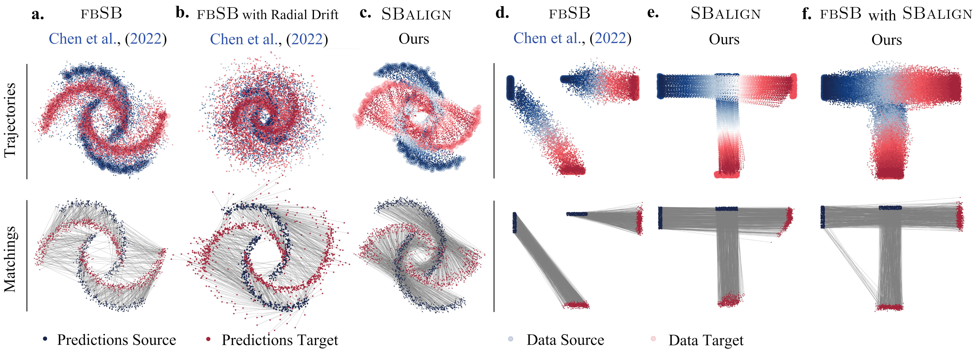
Figure 2: Experimental results on the Moon dataset (a-c) and T-dataset (d-f). The top row shows the trajectory sampled using the learned drift, and the bottom row shows the matching based on the learnt drift. Compared to other baselines, SBalign is able to learn an appropriate drift respecting the true alignment. (f) further showcases the utility of SBalign’s learnt drift as a suitable reference process to improve other training methods.

Regularization.

Since it is well-known that $\nabla\log h_{t}$ typically explodes when $t\to 1$ (Liu et al., 2023), it is important to regularize the behavior of $m^{\phi}$ for numerical stability, especially when $t\to 1$. Moreover, in practice, it is desirable to learn a drift $b_{t}^{\theta}$ that respects the data alignment in expectation: If $(\mathbf{x}_{0},\mathbf{x}_{1})$ is an input pair, then multiple runs of the SDE (5) starting from $\mathbf{x}_{0}$ should, on average, produce samples that are in the proximity of $\mathbf{x}_{1}$. This observation implies that we should search for drifts whose corresponding $h$-transforms are diminishing.

A simple way to simultaneously achieve the above two requirements is to add an $\ell^{2}$-regularization term, resulting in the loss function:

$$L(\theta,\phi) \vcentcolon=\mathbb{E}\Bigg{[}\int_{0}^{1}\left\lVert\frac{\mathbf{x}_{1}-X_{t}}{\beta_{1}-\beta_{t}}-\left(b_{t}^{\theta}+m^{\phi}(X_{t})\right)\right\rVert^{2}$$ (12)

$$\hskip 99.58464pt+\lambda_{t}\lVert m^{\phi}(\mathbf{x}_{t})\rVert^{2}\>\mathrm{d}t\Bigg{]}$$

where $\lambda_{t}$ can either be constant or vary with time. The overall algorithm is depicted in Algorithm 1.

3.2 Paired Schrödinger bridges as prior processes

Our algorithm finds solutions to SBs on aligned data by relying on samples drawn from the (optimal) coupling $\pi^{\star}$. This is what differentiates it from classical SBs –which instead only consider samples from $\hat{\mathbb{P}}_{0}$ and $\hat{\mathbb{P}}_{1}$– and plays a critical role in avoiding IPF-like iterates. However, SBalign reliance on samples from $\pi^{\star}$ may become a limitation, when the available information on alignments is insufficient.

If the number of pairings is limited, it is unrealistic to hope for an accurate solution to the aligned SB problem. However, the interpolation between $\hat{\mathbb{P}}_{0}$ and $\hat{\mathbb{P}}_{1}$ learned by SBalign can potentially be leveraged as a starting point to obtain a better reference process, which can then be used when solving a classical SB on the same marginals. In other words, the drift $b^{\text{aligned}}_{t}(X_{t})$ learned through SBalign can be used as is to construct a data-informed alternative $\tilde{\mathbb{Q}}$ to the standard Brownian motion, defined by paths:

$$\tilde{X}_{t}=b^{\text{aligned}}_{t}(\tilde{X}_{t})dt+g_{t}dW_{t}$$

Intuitively, solving a standard SB problem with $\tilde{\mathbb{Q}}$ as reference is beneficial because the (imperfect) coupling of marginals learned by SBalign ($\tilde{\mathbb{Q}}_{01}$) is, in general, closer to the truth than $\mathbb{Q}_{01}$.

Improving reference processes through pre-training or data-dependent initialization has been previously considered in the literature. For instance, both De Bortoli et al. (2021) and Chen et al. (2022a) use a pre-trained reference process for challenging image interpolation tasks. This approach, however, relies on DSBs trained using the classical score-based generative modeling objective between a Gaussian and the data distribution. It, therefore, pre-trains the reference process on a related –but different– process, i.e., the one mapping Gaussian noise to data rather than $\hat{\mathbb{P}}_{0}$ to $\hat{\mathbb{P}}_{1}$. An alternative, proposed by Bunne et al. (2023) draws on the closed-form solution of SBs between two Gaussian distributions, which are chosen to approximate $\hat{\mathbb{P}}_{0}$ and $\hat{\mathbb{P}}_{1}$, respectively. Unlike our method, these alternatives construct prior drifts by falling back to simpler and related tasks, or approximations of the original problem. We instead propose to shape a coarse-grained description of the drift based on alignments sampled directly from $\pi^{\star}_{01}$.

4 Experiments

In this section, we evaluate SBalign in different settings involving 2-dimensional synthetic datasets, the task of reconstructing cellular differentiation processes, as well as predicting the conformation of a protein structure and its ligand formalized as rigid protein docking problem.

4.1 Synthetic Experiments

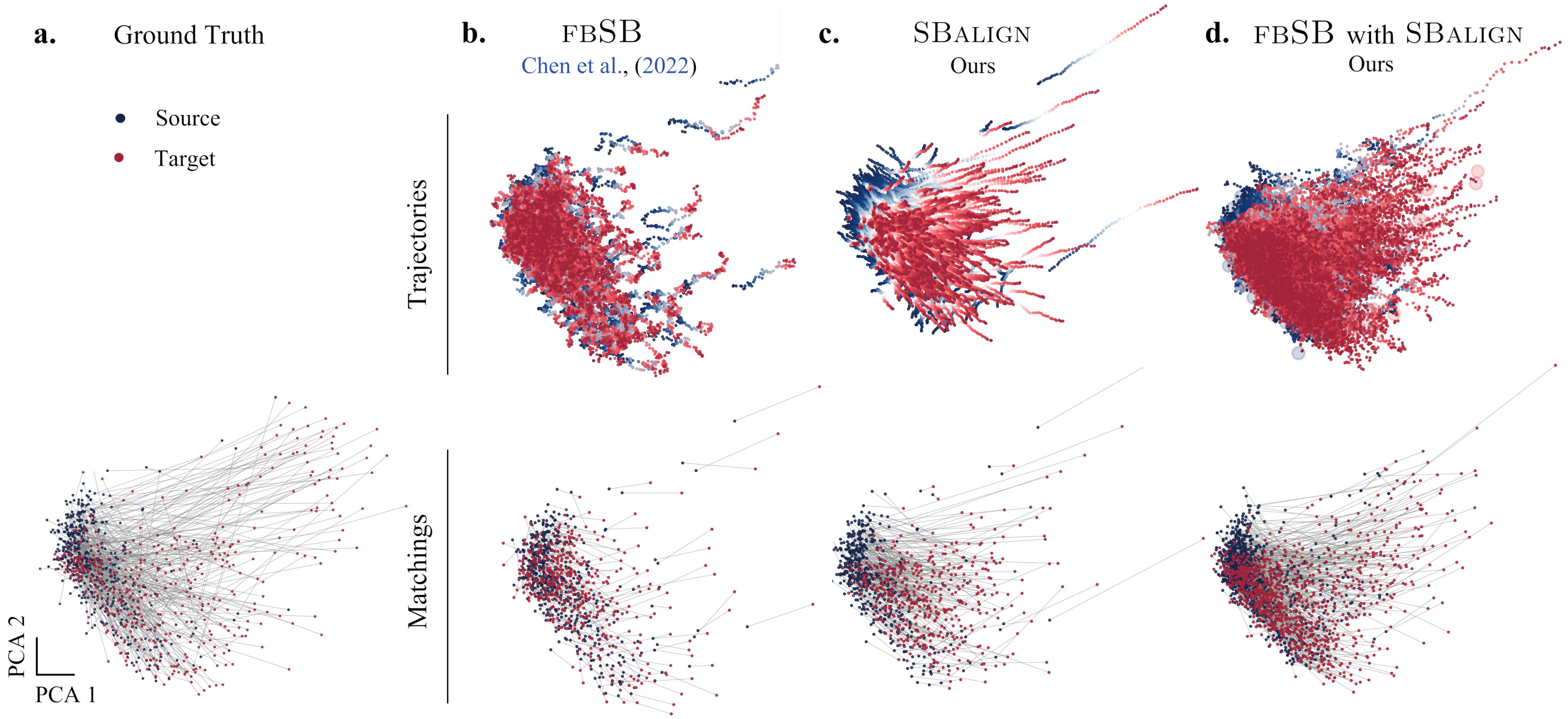
Figure 3: Cell differentiation trajectories based on (a) the ground truth and (b-d) learned drifts. SBalign is able to learn an appropriate drift underlying the true differentiation process while respecting the alignment. (d) Using the learned drift from SBalign as a reference process helps improve the drift learned by other training methods.

We run our algorithm on two synthetic datasets (Figures in § B), and compare the results with classic diffusion Schrödinger bridge models, i.e., the forward-backward SB formulation proposed by Chen et al. (2022a), herein referred to as fbSB. We equip the baseline with prior knowledge, as elaborated below, to further challenge SBalign.

Moon dataset.

The first synthetic dataset (Fig. 2a-c) consists of two distributions, each supported on two semi-circles ($\hat{\mathbb{P}}_{{0}}$ drawn in blue and $\hat{\mathbb{P}}_{{1}}$ in red). $\hat{\mathbb{P}}_{{1}}$ was obtained from $\hat{\mathbb{P}}_{{0}}$ by applying a clockwise rotation around the center, i.e., by making points in the upper blue arm correspond to those in the right red one. This transformation is clearly not the most likely one under the assumption of Brownian motion of particles and should therefore not be found as the solution of a classical SB problem. This is confirmed by fbSB trajectories (Fig. 2a), which tend to map points to their closest neighbor in $\hat{\mathbb{P}}_{{1}}$ (e.g., some points in the upper arm of $\hat{\mathbb{P}}_{{0}}$ are brought towards the left rather than towards the right). While being a minimizer of (SB), such a solution completely disregards our prior knowledge on the alignment of particles, which is instead reliably reproduced by the dynamics learned by SBalign (Fig. 2c).

One way of encoding this additional information on the nature of the process is to modify $\mathbb{Q}_{t}$ by introducing a clockwise radial drift, which describes the prior tangential velocity of particles moving circularly around the center. Solving the classical SB with this updated reference process indeed generates trajectories that respect most alignments (Fig. 2b), but requires a hand-crafted expression of the drift that is only possible in very simple cases.

T dataset.

In most real-world applications, it is very difficult to define an appropriate reference process $\mathbb{Q}_{t}$, which respects the known alignment without excessively distorting the trajectories from a solution to (SB). This is already visible in simple examples like (Fig. 2d-f), in which the value of good candidate prior drifts at a specific location needs to vary wildly in time. In this dataset, $\hat{\mathbb{P}}_{{0}}$ and $\hat{\mathbb{P}}_{{1}}$ are both bi-modal distributions, each supported on two of the four extremes of an imaginary T-shaped area. We target alignments that connect the two arms of the T as well as the top cloud with the bottom one. We succeed in learning them with SBalign (Fig. 2e) but unsurprisingly fail when using the baseline fbSB (Fig. 2d) with a Brownian motion prior.

In this case, however, attempts at designing a better reference drift for fbSB must take into account the additional constraint that the horizontal and vertical particle trajectories intersect (see Fig. 2e), i.e., they cross the same area at times $t_{h}$ and $t_{v}$ (with $t_{h}>t_{v}$). This implies that the drift $b_{t}$, which initially points downwards (when $t<t_{v}$), should swiftly turn rightwards (for $t>t_{h}$). Setting imprecise values for one of $t_{h}$ and $t_{v}$ when defining custom reference drifts for classical SBs would hence not lead to the desired result and, worse, would actively disturb the flow of the other particle group.

As described in § 3.2, in presence of hard-to-capture requirements on the reference drift, the use of SBalign offers a remarkably easy and efficient way of learning a parameterization of it. For instance, when using the drift obtained by SBalign as reference drift for the computation of the SB baseline (fbSB), we find the desired alignments (Fig. 2f).

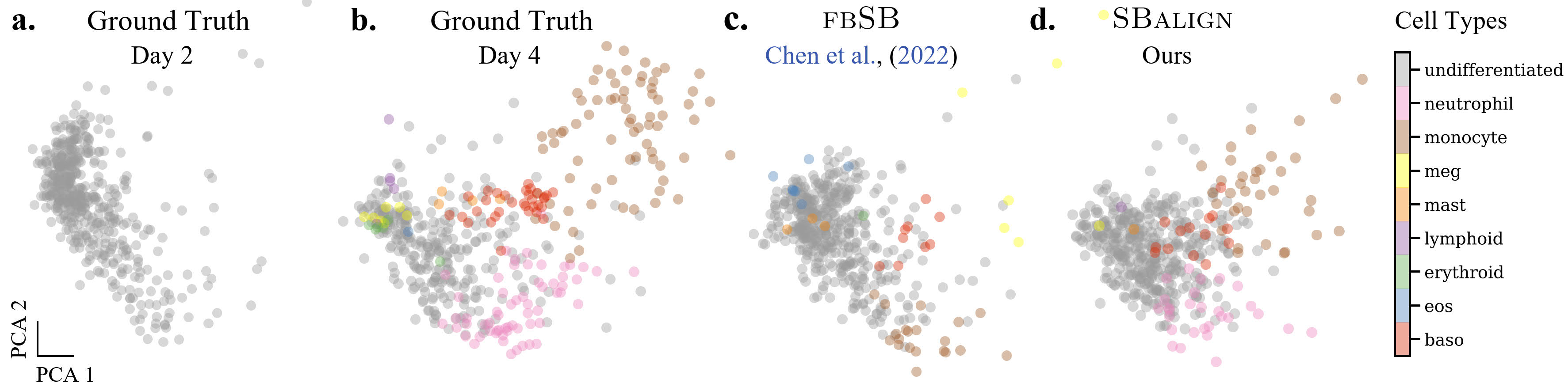
Figure 4: Cell type prediction on the differentiation dataset. All distributions are plotted on the first two principal components. a-b: Ground truth cell types on day 2 and day 4 respectively. c-d: fbSB and SBalign cell type predictions on day 4. SBalign is able to better model the underlying differentiation processes and capture the diversity in cell types.

4.2 Cell Differentiation

Biological processes are determined through heterogeneous responses of single cells to external stimuli, i.e., developmental factors or drugs. Understanding and predicting the dynamics of single cells subject to a stimulus is thus crucial to enhance our understanding of health and disease and the focus of this task. Most single-cell high-throughput technologies are destructive assays —i.e., they destroy cells upon measurement— allowing us to only measure unaligned snapshots of the evolving cell population. Recent methods address this limitation by proposing (lower-throughput) technologies that keep cells alive after transcriptome profiling (Chen et al., 2022b) or that genetically tag cells to obtain a clonal trace upon cell division (Weinreb et al., 2020).

Dataset.

To showcase SBalign’s ability to make use of such (partial) alignments when inferring cell differentiation processes, we take advantage of the genetic barcoding system developed by Weinreb et al. (2020). With a focus on fate determination in hematopoiesis, Weinreb et al. (2020) use expressed DNA barcodes to clonally trace single-cell transcriptomes over time. The dataset consists of two snapshots: the first, recorded on day 2, when most cells are still undifferentiated (see Fig. 4a), and a second, on day 4, comprising many different mature cell types (see Fig. 4b). Using SBalign as well as the baseline fsSB, we attempt to reconstruct cell evolution between day 2 and day 4, all while capturing the heterogeneity of emerging cell types. For details on the dataset, see § B.

Table 1: Cell differentiation prediction results. Means and standard deviations (in parentheses) of distributional metrics (maximum-mean-discrepancy (MMD), $\text{W}_{\epsilon}$), alignment-based metrics ($\ell_{2}$, RMSD), and cell type classification accuracy.

Cell Differentiation Methods MMD $\downarrow$ $\text{W}_{\varepsilon}\downarrow$ $\ell_{2}(\text{PS})\downarrow$ RMSD $\downarrow$ Class. Acc. $\uparrow$ fbSB 1.55e-2 (0.03e-2) 12.50 (0.04) 4.08 (0.04) 9.64e-1 (0.02e-1) 56.2% (0.7%) fbSB with SBalign 5.31e-3 (0.25e-3) 10.54 (0.08) 0.99 (0.12) 9.85e-1 (0.07e-1) 47.0% (1.5%) SBalign 1.07e-2 (0.01e-2) 11.11 (0.02) 1.24 (0.02) 9.21e-1 (0.01e-1) 56.3% (0.7%)

Baselines.

We benchmark SBalign against previous DSBs such as (Chen et al., 2022a, fbSB). Beyond, we compare SBalign in the setting of learning a prior reference process. Naturally, cell division processes and subsequently the propagation of the barcodes are very noisy. While this genetic annotation provides some form of assignment, it does not capture the full developmental process. We thus test SBalign in a setting where it learns a prior from such partial alignments and, plugged into fbSB, is fine-tuned on the full dataset.

Evaluation metrics.

To assess the performance of SBalign and the baselines, we monitor several metrics, which include distributional distances, i.e., MMD (Gretton et al., 2012) and $\text{W}_{\epsilon}$ (Cuturi, 2013), as well as average (perturbation scores), i.e., $\ell_{2}(\text{PS})$ (Bunne et al., 2022a) and RMSD. Moreover, we also train a simple neural network-based classifier to annotate the cell type on day 4 and we report the accuracy of the predicted vs. actual cell type for all the models. See § C.1 for further details.

Results.

SBalign finds matching between cell states on days 2 and 4 (Fig. 3c, bottom) which resemble the observed ones (Fig. 3a) but also reconstructs the entire evolution path of transcriptomic profiles (Fig. 3c, top). It outperforms the baseline fbSB (Table 1) in all metrics: Remarkably, our method exceeds the performances of the baseline also on distributional metrics and not uniquely on alignment-based ones. We also leverage SBalign predictions to recover the type of cells at the end of the differentiation process (Fig. 4d). We do that by training a classifier on differentiated cells observed on day 4, and subsequently classify our predictions. While capturing the overall differentiation trend, SBalign (as well as fbSB) struggles to isolate rare cell types. Lastly, we employ SBalign to learn a prior process from noisy alignments based on genetic barcode annotations. When using this reference process within fbSB, we learn an SB which compensates for inaccuracies stemming from the stochastic nature of cell division and barcode redistribution and which achieves better scores on distributional metrics (see Tab. 1). Further results can be found in § A.

4.3 Protein Docking

Proteins are dynamic, flexible biomolecules that form complexes upon interaction with other biomolecules. This is a central step in many biological processes, namely signal transduction, DNA replication, and repair. The formation of complexes is guided by appropriate energetics, best orienting the participating proteins relative to each other, along with a dynamic alteration in structure (conformational changes) to form a stable complex.

Understanding the mechanistic principles governing this process is thus a central problem in biology, with the goal of engineering protein interactions to achieve a desired functional or therapeutic response. In (computational) protein docking, the goal is to predict the 3D structure of the bound (docked) state of a protein pair, given the unbound states of the corresponding proteins. These proteins are denoted (arbitrarily) as the ligand and receptor respectively.

A comprehensive treatment of the protein docking problem is still elusive, owing to the lack of high-quality large datasets comprising 3D structures of participating proteins in the unbound and bound states. We tackle, instead, two related subproblems: (i) the prediction of conformational changes between unbound and bound states of proteins and (ii) the identification of the best orientation between interacting proteins, modelled as rigid bodies. This separation into related subproblems was also adopted in (Dominguez et al., 2003), one of the earliest works for the full protein docking problem.

4.3.1 Conformational Changes in Proteins

This task involves modeling the conformational changes between the unbound and bound states of proteins. More formally, given the 3D structure of an unbound protein, we predict its 3D structure in the bound state. While it is possible to frame this problem as a (conditional) point cloud translation, an approach using Schrödinger bridges is more natural since it leverages the dynamic and flexible nature of proteins and accounts for the underlying stochasticity in the conformational change process.

Dataset.

The task of modeling conformational changes starting from a given protein structure is largely unexplored, mainly due to the lack of high-quality large datasets. Here we utilize the recently proposed D3PM dataset (Peng et al., 2022) that provides protein structures before (apo) and after (holo) binding, covering various types of protein motions. The dataset was generated by filtering examples from the Protein Data Bank (PDB) corresponding to the same protein but bound to different biomolecules, with additional quality control criteria. For the scope of this work, we only focus on protein pairs where the provided Root Mean Square Deviation (RMSD) of the C$\alpha$ carbon atoms between unbound and bound 3D structures is $>3.0$Å, which amounts to 2370 examples in the D3PM dataset.

For each pair of structures, we first identify common residues, and compute the RMSD between C$\alpha$ carbon atoms of the common residues after superimposing them using the Kabsch (Kabsch, 1976) algorithm, and only accept the structure if the computed C$\alpha$ RMSD is within a certain margin of the provided C$\alpha$ RMSD. The rationale behind this step is to only retain examples where we can reconstruct the RMSD values provided with the dataset. The above preprocessing steps give us a dataset with 1591 examples, which is then divided into a train/valid/test split of 1291/150/150 examples respectively. More details in § B.3.1.

Baselines.

Since the goal of the task is to predict 3D structures, our model must satisfy the relevant SE(3) symmetries of rotation and translations. To this end, we evaluate SBAlign against the EGNN model (Satorras et al., 2021), which satisfies the SE(3) symmetries and is a popular architecture used in many point-cloud transformation tasks (Satorras et al., 2021; Hoogeboom et al., 2022). In particular, we consider the variant of the EGNN model proposed in Xu et al. (2022), owing to its strong performance on the molecule conformer generation task.

Results.

To evaluate our model, we report (Table 2) summary statistics of the RMSD between the C$\alpha$ carbon atoms of the predicted structure and the ground truth, and the fraction of predictions with RMSD values $<2.0,5.0$ and $10.0$Å. SBAlign outperforms EGNN by a large margin and is able to predict almost 70% examples with an RMSD$<5$Å. One of the drawbacks attributed to diffusion models is their slow sampling speed, owing to multiple function calls to a neural network. Remarkably, our model is able to achieve impressive performance with just 10 steps of simulation. We leave it to future work to explore the tradeoff between sampling speed and quality (as measured by RMSD) of the predicted conformations.

Table 2: Conformational changes results. RMSD between predicted and true structures in the bound state. The first term in the parentheses refers to the number of poses sampled, and the second term refers to the simulation steps for the trajectory.

D3PM Test Set RMSD (Å) % RMSD (Å) $<\tau$ Methods Median Mean Std $\tau=2$ $\tau=5$ $\tau=10$ EGNN 19.99 21.37 8.21 1% 1% 3% SBAlign (10, 10) 3.80 4.98 3.95 0% 69% 93% SBAlign (10, 100) 3.81 5.02 3.96 0% 70% 93%

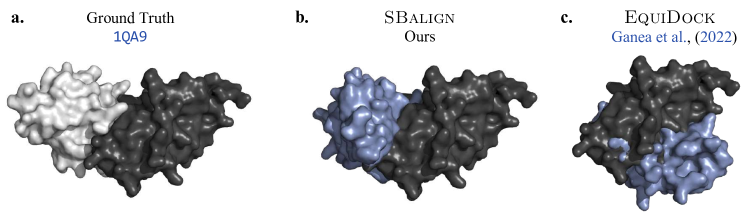
Figure 5: Ground truth and predicted bound structures for the complex with PDB ID: 1QA9. SBalign is able to find the true binding interface compared to EquiDock.

4.3.2 Rigid Protein Docking

Experimental setup.

Our setup follows a similar convention as EquiDock (Ganea et al., 2022). To summarize, the unbound structure of the ligand is derived by applying a random rotation and translation to the corresponding bound structure, while the receptor is held fixed w.l.o.g. Applying a different rotation and translation to each ligand can however result in a different Brownian bridge for each complex, resulting in limited meaningful signal for learning $b_{t}^{\theta}$. To avoid this, we sample a rotation and translation at the start of training and apply the same rotation and translation to all complexes across training, validation, and testing. Additional details regarding this setup can be found in § B.

Dataset.

For our empirical evaluation, we use the DB5.5 dataset (Vreven et al., 2015) which is a standard choice for protein-protein docking but contains only 253 complexes. We utilize the same splits as EquiDock (Ganea et al., 2022), with 203 complexes in the training set, 25 complexes in the validation set, and 25 complexes in the test set. For the evaluation in Table 3, we use the full DB5.5 test set. For ligands in the test set, we generate the corresponding unbound versions by applying the rotation and translation sampled during training. We compare our method to the GNN-based model EquiDock as well as traditional docking software, see § A.2 for details.

Evaluation metrics.

We report two metrics, complex root mean square deviation (Complex RMSD), and interface root mean square deviation (Interface RMSD). Following (Ganea et al., 2022), the ground truth and predicted complex structures are first superimposed using the Kabsch algorithm (Kabsch, 1976), and the Complex RMSD is then computed between the superimposed versions. A similar procedure is used for computing Interface RMSD, but only using the residues from the two proteins that are within $8\,$Å of each other. More details in § C.1.

Results.

SBalign considerably outperforms EquiDock across all metrics (Table 3). Our method also achieves comparable or better performance than traditional docking software without relying on extensive candidate sampling and re-ranking or learning surface templates from parts of the current test set. An example of docked structures, in direct comparison with EquiDock is displayed Fig. 5. Further visualizations and results can be found in § A.

Table 3: Rigid docking results. Complex and interface RMSD between predicted and true bound structures (after Kabsch alignment). Comparison with values reported in (Ganea et al., 2022) can be found in § A.2.

DB5.5 Test Set Complex RMSD Interface RMSD Methods Median Mean Std Median Mean Std EquiDock 14.12 14.73 5.31 11.97 13.23 4.93 SBalign 6.59 6.69 2.04 7.69 8.11 2.39

Future outlook.

In this section, we presented a proof of concept application of SBAlign for the subproblems associated with the protein docking task. While SBAlign provides a principled method to model conformational changes between unbound and bound states of a protein, our setup for rigid protein docking is limited by utilizing the same rotation and translation across training and testing. A combination of SBAlign for conformational change modeling, with more recent methods for rigid-protein docking (Ketata et al., 2023) can provide a complete solution for the protein docking task, which we leave to future work.

5 Conclusion

In this paper, we propose a new framework to tackle the interpolation task with aligned data via diffusion Schrödinger bridges. Our central contribution is a novel algorithmic framework derived from the Schrödinger bridge theory and Doob’s $h$-transform. Via a combination of the two notions, we derive novel loss functions which, unlike all prior methods for solving diffusion Schrödinger bridges, do not rely on the iterative proportional fitting procedure and are hence numerically stable. We verify our proposed algorithm on various synthetic and real-world tasks and demonstrate noticeable improvement over the previous state-of-the-art, thereby substantiating the claim that data alignment is a highly relevant feature that warrants further research.

Appendix A Additional Results

A.1 Variance Reduction

In this paragraph, we elaborate on the need to parametrize also Doob’s $h_{t}$ function, along with the drift $b_{t}$. Introducing $m^{\phi}$ removes the need to evaluate (11) which is difficult to approximate in practice on high-dimensional spaces. This equation amounts, in fact, to a Gaussian Kernel Density Estimation of the conditional probability $\operatorname{\mathbb{P}}(X_{1}=\mathbf{x}_{1}|X_{t}=\mathbf{x})$ along (unconditional) paths obtained from (5). Faithful approximations of (11) would, therefore, require:

• good-quality paths, which are scarce at the beginning of training when the drift $b_{t}^{\theta}$ has not yet been learned;

• exponentially many trajectories (in the dimension of the state space);

• that points $x_{1}$ (obtained from conditional trajectories, Eq. 6) be reasonably close to $x_{1}$ (obtained from unconditional trajectories, Eq. 5);

Even if all the above conditions were satisfied, the quantity $h_{t}(x)=\operatorname{\mathbb{P}}(X_{1}=\mathbf{x}_{1}|X_{t}=\mathbf{x})$ would still be challenging to directly manipulate. It is, in fact, much smaller at earlier times $t$ (see Table 4), since knowledge of the far past has a weaker influence on the location $X_{1}$ of particles at time $t=1$. Precision errors at $t\approx 0$ would then be amplified when computing the score of $h_{t}$ (i.e, $\nabla\log h_{t}$) –which appears in the loss (8)– and accumulate over timesteps, eventually leading trajectories astray. By directly parameterizing the score, we instead sidestep this problem. The magnitude of $m^{\phi}_{t}\approx\nabla\log h_{t}$ can, in fact, be more easily controlled and regularized.

	Time $t$
	0	0.15	0.30	0.45	0.60	0.75	0.90
Mean $h_{t,\tau}$ value	2.92e-14	4.03e-13	2.54e-11	1.72e-09	1.47e-07	2.66e-05	8.53e-3

Table 4: Average $h_{t,\tau}$ values along paths, at different timesteps. $\operatorname{\mathbb{P}}(X_{1}=\mathbf{x}_{1}|X_{t}=\mathbf{x})$ ranges over 11 orders of magnitude across the time interval and is smallest when $t\approx 0$.

A.2 Rigid Protein Docking

Baselines.

We compare our method to EquiDock as well as traditional docking software including Attract (Schindler et al., 2017; de Vries et al., 2015), HDock (Yan et al., 2020), ClusPro (Desta et al., 2020; Kozakov et al., 2017), and PatchDock (Mashiach et al., 2010; Schneidman-Duhovny et al., 2005). As mentioned in the paragraph above, for ligands in the test set, we generate the corresponding unbound versions by applying the rotation and translation sampled during training. We evaluate the trained model from EquiDock and SBalign on these unbound structures and report corresponding evaluation metrics. For the remaining baselines, we include the numbers from (Ganea et al., 2022). These baselines typically sample several candidate complexes by considering small increments of rotation angles. We expect this makes them somewhat invariant to arbitrary initialization, and the corresponding docking scores to not be severely impacted.

Table 5: Rigid docking results. Complex and interface RMSD between predicted and true bound structures (after Kabsch alignment). ^∗ denotes methods for which we use values directly from (Ganea et al., 2022). All other results show the performance on our test set.

DB5.5 Test Set Complex RMSD Interface RMSD Methods Median Mean Std Median Mean Std Attract^∗ 9.55 10.09 9.88 7.48 10.69 10.90 HDock^∗ 0.30 5.34 12.04 0.24 4.76 10.83 ClusPro^∗ 3.38 8.25 7.92 2.31 8.71 9.89 PatchDock^∗ 18.26 18.00 10.12 18.88 18.75 10.06 EquiDock^∗ 14.13 14.72 5.31 11.97 13.23 4.93 EquiDock 14.12 14.73 5.31 11.97 13.23 4.93 SBalign 6.59 6.69 2.04 7.69 8.11 2.39

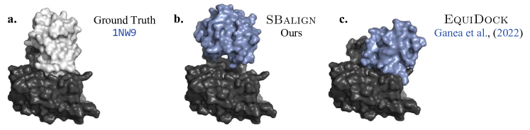
Figure 6: Ground truth and predicted bound structures for the complex with PDB ID: 1NW9. SBalign is able to identify the true binding pocket.

Results.

The model performance is summarized in Table 5. Our method SBalign considerably outperforms EquiDock across all metrics. SBalign also achieves comparable or better performance than traditional docking software without relying on extensive candidate sampling and re-ranking or learning surface templates from parts of the current test set. An example of docked structures, in direct comparison with EquiDock is displayed Fig. 5. Beyond the results in Table 5, we display the ground truth and docked complexes in Figs. 5, 6, and 7.

Figure 7: Ground truth and predicted bound structures for the complex with PDB ID: 1JIW. SBalign is able to find the true binding interface compared to EquiDock.

Appendix B Datasets

B.1 Synthetic Datasets

In the following, we provide further insights and experimental results in order to access the performance of SBalign in comparison with different baselines and across tasks of various nature. For each dataset, we describe in detail its origin as well as preprocessing and featurization steps.

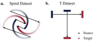
Figure 8: Initial (blue) and final (red) marginals for the two toy datasets (a) moon and (b) T, together with arrows indicating a few alignments

Moon dataset.

The moon toy dataset (Fig. 8a) is generated by first sampling $\hat{\mathbb{P}}_{{1}}$ and then applying a clockwise rotation of $233^{\circ}$ around the origin to obtain $\hat{\mathbb{P}}_{{0}}$. The points on the two semi-circumferences supporting $\hat{\mathbb{P}}_{{1}}$ are initially placed equally-spaced along each semi-circumference and then moved by applying additive Gaussian noise to both coordinates. While classic generative models will choose the shortest path and connect ends of both moons closest in Euclidean distance, only methods equipped with additional knowledge or insight on the intended alignment will be able to solve this task.

T dataset.

This toy dataset (Fig. 8b) is generated by placing an equal amount of samples at each of the four extremes of a T-shaped area having ratio between x and y dimensions equal to 51/55. If run with a Brownian prior, classical SBs also fail on this dataset because they produce swapped pairings: i.e., they match the left (resp. top) point cloud with the bottom (resp. right) one. At the same time, though, this dataset prevents reference drifts with simple analytical forms (such as spatially-symmetric or time-constant functions) from fixing classical SBs runs. It therefore illustrates the need for general, plug-and-play methods capable of generating approximate reference drifts to use in the computation of classical SBs.

B.2 Cell Differentiation Datasets

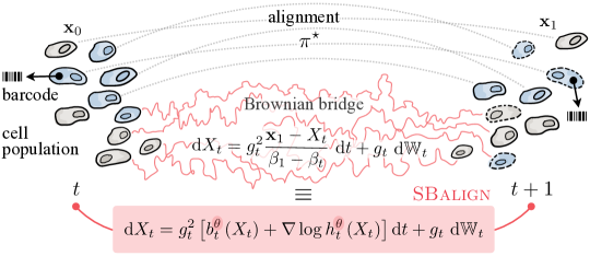
Figure 9: Overview of SBalign in the setting of cell differentiation with the goal of learning the evolutionary process that morphs a population from its stat at $t$ to $t+1$. Through genetic tagging (i.e., barcodes) we are able to trace progenitor cells at time point $t$ into their descendants $t+1$. This provides us with an alignment between populations at consecutive time steps. Our goal is then to recover a stochastic trajectory from $\mathbf{x}_{0}$ to $\mathbf{x}_{1}$. To achieve this, we connect the characterization of a SDE conditioned on $\mathbf{x}_{0}$ and $\mathbf{x}_{1}$ (utilizing the Doob’s $h$-transform) with that of a Brownian bridge between $\mathbf{x}_{0}$ and $\mathbf{x}_{1}$ (classical Schrödinger bridge theory), leading to a simpler training procedure with lower variance and strong empirical results.

Dataset description.

We obtain the datapoints used in our cell differentiation task from the dataset generated by Weinreb et al. (2020), which contains 130861 observations/cells. We follow the preprocessing steps in Bunne et al. (2021) and use the Python package scanpy (Wolf et al., 2018). After processing, each observation records the level of expression of 1622 different highly-variable genes as well as the following meta information per cell:

• a timestamp, expressed in days and taking values in {2, 4, 6};

• a barcode, which is a short DNA sequence that allows tracing the identity of cells and their lineage by means of single-cell sequencing readouts;

• an additional annotation, which describes the current differentiation fate of the cell.

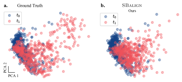
Figure 10: Distribution of the cell population (i.e., marginals) at time $t=t_{0}$ and $t=t_{1}$ for (a) the ground truth, and (b) SBalign, after projection along their first two principal components.

Dataset preparation.

We only retain cells with barcodes that appear both on days 2 and 4, taking care of excluding cells that are already differentiated on day 2. We construct matchings by pairing cells measured at two different times but which share the barcode. Additionally, we filter cells to make sure that no one appears in more than one pair. To reduce the very high dimensionality of these datapoints, we perform a PCA projection down to 50 components.

We end up with a total of 4702 pairs of cells, which we partition into train, validation, and test sets according to the split 80%/10%/10%.

B.3 Protein Docking

B.3.1 Conformational Changes

Dataset description.

For the task of predicting protein conformational changes, we utilize the D3PM dataset. The dataset consists of both unbound and bound structures for 4330 proteins, under different types of protein motions. The PDB IDs were downloaded from https://www.d3pharma.com/D3PM/. For the PDB IDs making up the dataset, we download the corresponding (.cif) files from the Protein Data Bank.

Dataset preparation.

For the scope of this work, we only focus on protein structure pairs, where the provided RMSD between the C$\alpha$ carbon atoms is $>3$Å, amounting to 2370 examples in the D3PM dataset. For each pair of structures, we first identify common residues, and compute the RMSD between C$\alpha$ carbon atoms of the common residues after superimposing them using the Kabsch (Kabsch, 1976) algorithm, and only accept the structure if the computed C$\alpha$ RMSD is within a certain margin of the provided C$\alpha$ RMSD. The rationale behind this step was to only retain examples where we could reconstruct the RMSD values provided with the dataset. Common residues are identified through a combination of residue position and name. This step is however prone to experimental errors, and we leave it to future steps to improve the common residue identification step (using potentially, a combination of common subsequences and/or residue positions).

After applying the above preprocessing steps, we obtain a dataset with 1591 examples, which is then split into a train/valid/test split of 1291/150/150 examples respectively. The structures used in training and inference are the Kabsch superimposed versions, therefore ensuring that the Brownian bridges are sampled between the unbound and bound states of the proteins, and no artifacts are introduced by 3D rotations and translations, which do not contribute to conformational changes.

Featurization.

Following standard practice and for memory and computational efficiency, we only use the C$\alpha$ coordinates of the residues to represent our protein structures instead of the full-atom structures. For each amino acid residue, we compute the following features: a one hot encoding of the amino acid identity $f_{e}$ of size $23$, hydrophobicity $f_{h}\in[-4.5,4.5]$, volume $f_{v}\in[60.1,227.8]$, the charge $f_{c}\in\{-1,0,1\}$, polarity $f_{p}\in\{0,1\}$, and whether the amino acid residue is a hydrogen bond donor $f_{d}\in\{0,1\}$ or acceptor $f_{a}\in\{0,1\}$. The hydropathy and volume features are expanded into a radial basis with interval sizes $0.1$ and $10$ respectively. To equip the model with a notion of time, we use a sinusoidal embedding of time $\phi(t)$ of embedding dimensionality $32$. These are concatenated to the amino acid features to form our input features for the amino acid residues. The edge features consist of a radial basis expansion of the distances between the residues. We also compute the spherical harmonics of the edge vectors between the residues, which is used in the tensor product message passing layers.

Position at t.

For any time $t$, we sample the positions of the C$\alpha$ atoms using the Brownian Bridge - given the coordinates $\mathbf{x}_{0}$ at $t=0$ and the coordinates $\mathbf{x}_{1}$ at $t=1$ with a Brownian bridge between $\mathbf{x}_{0}$ and $\mathbf{x}_{1}$, we know that $x_{t}\sim\mathcal{N}\left(x_{t};(1-t)\mathbf{x}_{0}+t\mathbf{x}_{1},t(1-t)\right)$.

B.3.2 Rigid Protein Docking

Dataset description.

We use the DB5.5 dataset (Vreven et al., 2015) for our empirical evaluation. The DB5.5 dataset is a standard dataset used in protein-protein docking, however, it only has 253 complexes. The dataset was downloaded from https://zlab.umassmed.edu/benchmark/. The dataset consists of both unbound and bound structures, but the structures are largely rigid, with an average complex RMSD of 0.96 between the bound and unbound structures. We utilize the same splits as EquiDock (Ganea et al., 2022), with 203 complexes in the training set, 25 complexes in the validation set, and 25 complexes in the test set. For the evaluation in Table 5, we use the full DB5.5 test set. For ligands in the test set, we generate the corresponding unbound versions by applying the rotation and translation sampled during training.

Dataset preparation.

Following similar convention as EquiDock (Ganea et al., 2022), we treat the receptor as fixed. For each ligand, the final 3D structure corresponds to its bound version, and the unbound version is generated by applying a random rotation $R$ and translation $b$ to the bound version. However, applying a different rotation and translation to each ligand would result in a different Brownian bridge, thus providing limited learning signal for the drift $b_{t}^{\theta}$. To avoid this, we create a rotation matrix $R$ during training by sampling a random angle between $30-45^{\circ}$ along each axis, and a translation $b$ with a maximum magnitude between $5.0-10.0$. The same $R$ and $b$ are also applied to the validation and test sets. We leave it to future work to extend the algorithm to work for arbitrary rotations and translations.

Featurization.

Following standard practice and for memory and computational efficiency, we only use the C$\alpha$ coordinates of the residues to represent our protein structures instead of the full-atom structures. For each amino acid residue, we compute the following features: a one hot encoding of the amino acid identity $f_{e}$ of size $23$, hydrophobicity $f_{h}\in[-4.5,4.5]$, volume $f_{v}\in[60.1,227.8]$, the charge $f_{c}\in\{-1,0,1\}$, polarity $f_{p}\in\{0,1\}$, and whether the amino acid residue is a hydrogen bond donor $f_{d}\in\{0,1\}$ or acceptor $f_{a}\in\{0,1\}$. The hydropathy and volume features are expanded into a radial basis with interval size $0.1$ and $10$ respectively. To equip the model with a notion of time, we use a sinusoidal embedding of time $\phi(t)$ of embedding dimensionality $32$. These are concatenated to the amino acid features to form our input features for the amino acid residues.

Position at t.

For any time $t$, we sample the positions of the C$\alpha$ atoms using the Brownian Bridge - given the coordinates $\mathbf{x}_{0}$ at $t=0$ and the coordinates $\mathbf{x}_{1}$ at $t=1$ with a Brownian bridge between $\mathbf{x}_{0}$ and $\mathbf{x}_{1}$, we know that $x_{t}\sim\mathcal{N}\left(x_{t};(1-t)\mathbf{x}_{0}+t\mathbf{x}_{1},t(1-t)\right)$.

Appendix C Experimental Details

In the following, we provide further experimental details on the chosen evaluation metrics, network architectures, and hyperparameters.

C.1 Evaluation Metrics

C.1.1 Cell Differentiation

For fairness of comparison between our method and the baseline (fbSB) —which only works at the level of distribution of cells— we also consider three evaluation metrics (i.e., $W_{\varepsilon}$, MMD and $\ell_{2}$) that capture the similarity between the end marginal $\hat{\mathbb{P}}_{{1}}$ and our prediction $\pi^{\star}_{1}$, irrespective of matchings.

In what follows, we denote with $\hat{\nu}$ the predicted end marginal $\pi^{\star}_{1}$ —i.e., the predicted status of cells at day 4— and with $\nu$ the distribution of observed transcriptomes.

Wasserstein-2 distance.

We measure accuracy of the predicted target population $\hat{\nu}$ to the observed target population $\nu$ using the entropy-regularized Wasserstein distance (Cuturi, 2013) provided in the OTT library (Bradbury et al., 2018; Cuturi et al., 2022) defined as

(C.1)

where $H(\mathbf{P})\vcentcolon=-\sum_{ij}\mathbf{P}_{ij}(\log\mathbf{P}_{ij}-1)$ and the polytope $U(\hat{\nu},\nu)$ is the set of $n\times m$ matrices $\{\mathbf{P}\in\mathbb{R}^{n\times m}_{+},\mathbf{P}\mathbf{1}_{m}=\hat{\nu},\mathbf{P}^{\top}\mathbf{1}_{n}=\nu\}$.

Maximum mean discrepancy.

Kernel maximum mean discrepancy (Gretton et al., 2012) is another metric to measure distances between distributions, i.e., in our case between predicted population $\hat{\nu}$ and observed one $\nu$. Given two random variables $x$ and $y$ with distributions $\hat{\nu}$ and $\nu$, and a kernel function $\omega$, Gretton et al. (2012) define the squared MMD as:

$$\text{MMD}(\hat{\nu},\nu;\omega)=\mathbb{E}_{x,x^{\prime}}[\omega(x,x^{\prime})]+\mathbb{E}_{y,y^{\prime}}[\omega(y,y^{\prime})]-2\mathbb{E}_{x,y}[\omega(x,y)].$$

We report an unbiased estimate of $\text{MMD}(\hat{\nu},\nu)$, in which the expectations are evaluated by averages over the population particles in each set. We utilize the RBF kernel, and as is usually done, report the MMD as an average over the length scales: $2,1,0.5,0.1,0.01,0.005$.

Perturbation signature $\ell_{2}$.

A common method to quantify the effect of a perturbation on a population is to compute its perturbation signature (Stathias et al., 2018, (PS)), computed via the difference in means between the distribution of perturbed states and control states of each feature, e.g., here individual genes. $\ell_{2}$(PS) then refers to the $\ell_{2}$-distance between the perturbation signatures computed on the observed and predicted distributions, $\nu$ and $\hat{\nu}$. The $\ell_{2}$(PS) is defined as

$$\text{PS}(\nu,\mu)=\frac{1}{m}\sum_{y_{i}\in\nu}{y_{i}}-\frac{1}{n}\sum_{x_{i}\in\mu}{x_{i}},$$

where $n$ is the size of the unperturbed and $m$ of the perturbed population. We report the $\ell_{2}$ distance between the observed signature $\text{PS}(\nu,\mu)$ and the predicted signature $\text{PS}(\hat{\nu},\mu)$, which is equivalent to simply computing the difference in the means between the observed and predicted distributions.

RMSD.

To measure the quality of matchings sampled from SBalign $(\hat{x}^{i}_{0},\hat{x}^{i}_{1})$ —compared to the observed ones $(x^{i}_{0},x^{i}_{1})$— we compute:

$$\text{RMSD}(\{x^{i}_{1}\}^{n},\{\hat{x}^{i}_{1}\}^{n})=\sqrt{\frac{1}{n}\sum^{n}_{i=1}\lVert x^{i}_{1}-\hat{x}^{i}_{1}\rVert^{2}}$$ (C.2)

which, when squared, represents the mean of the square norm of the differences between predicted and observed statuses of the cells on day 4.

Cell type classification accuracy.

We assess the quality of SBalign trajectories by trying to predict the differentiation fate of cells, starting from (our compressed representation of) their transcriptome. For this, we train a simple MLP-based classifier on observed cells and use it on the last time-frame of trajectories sampled from SBalign to infer the differentiation of cells on day 4. We use the classifier MLPClassifier offered by the library scikit-learn with the following parameters:

• 2 hidden layers, each with a hidden dimension of 50,

• the logistic function as non-linearity

• $\ell_{2}$ norm, regularization with coefficient $0.1$.

We report the subset accuracy of the predictions on the test set, measured as the number of labels (i.e., cell types) coinciding with the ground truth.

C.1.2 Rigid Protein Docking

We report two metrics, Complex Root Mean Square Deviation (Complex RMSD), and Interface Root Mean Square Deviation (Interface RMSD). Following (Ganea et al., 2022), the ground truth and predicted complex structures are first superimposed using the Kabsch algorithm (Kabsch, 1976), and the Complex RMSD is then computed between the superimposed versions. A similar procedure is used for computing Interface RMSD, but only using the residues from the two proteins that are within $8\,$Å of each other. Given a ligand with $m$ residues and a receptor with $n$ residues, we denote the predicted bound structures with $\mathbf{Z}^{\prime}\in\mathbb{R}^{(n+m)}$ and the ground truth bound structure with $\mathbf{Z}^{*}\in\mathbb{R}^{(n+m)}$. We first superimpose the predicted and ground truth bound structures using the Kabsch algorithm and then compute the Complex RMSD as $\text{C}_{\text{rmsd}}=\sqrt{\frac{1}{n+m}\left\lVert\mathbf{Z}^{\prime}-\mathbf{Z}\right\rVert_{F}}$. The Interface RMSD $\text{I}_{\text{rmsd}}$ is computed similarly, but only using the residues from the two proteins that are within 8Å of each other.

C.2 Network Architectures

C.2.1 Cell Differentiation and Synthetic Datasets

We parameterize both $b^{\theta}(t,X_{t})$ and $m^{\phi}(t,b_{t},X_{t})$ using a model composed of:

1. x_enc: 3-layer MLP performing the expansion of spatial coordinates (or drift) into hidden states (of dimension 64 to 256);

2. t_enc: sinusoidal embedding of time (on 64 to 256 dimensions), followed by a two layer MLP;

3. mlp: 3-layer MLP which maps the concatenation of embedded spatial and temporal information (output of modules 1 and 2 above) to drift magnitude values along each dimension.

After every linear layer (except the last one), we apply a non-linearity and dropout (level 0.1). In all the experiments, we set the diffusivity function $g(t)$ in (5) to a constant $g$, which is optimized (see § C.3).

C.2.2 Protein Conformational Changes

As our architecture $b^{\theta}_{t}(X_{t})$ suitable for approximating the true drift $b_{t}$, we construct a graph neural networks with tensor-product message passing layers using e3nn (Thomas et al., 2018; Geiger and Smidt, 2022). To build the graph, we consider a maximum of 40 neighbors –located within a radius of 40Å for each residue. The model is SE(3) equivariant and receives node and edge features capturing relevant residue properties, and distance embeddings.

C.2.3 Rigid Protein Docking

For the scope of this paper, we use a MLP as $b_{t}^{\theta}$ and $m^{\phi}$. As inputs, both $b_{t}^{\theta}$ and $m^{\phi}$ receive input node features and the C_α coordinates at time $t$, as described in Section C.3.4, with $m^{\phi}$ receiving the prediction $b_{t}^{\theta}$ as additional input. Both models have $3$ hidden layers, each with a dimension of $64$ and an output dimension of $3$, with around 50K parameters in total. Our current architectures are not equivariant to global rotations and translations, which is a desirable property in protein docking as the structures of the proteins themselves are invariant to the choice of reference coordinates frames. We leave a thorough exploration of other architectures, such as equivariant GNN architectures similar to those adopted in (Ganea et al., 2022) to future work.

C.3 Hyperparameters

In the following, we will provide an overview of the selected hyperparameters as well as chosen training procedures.

C.3.1 Synthetic Tasks

We perform hyper-parameter optimization using the Python package ray.tune (Liaw et al., 2018) on:

• activation, chosen among leaky_relu, relu, selu and silu as implemented in the Python library PyTorch (Paszke et al., 2019). We find selu to achieve marginally better performance on toy datasets.

• g, the value of the diffusivity constant, chosen among $\{1,2,5,10\}$. We find $g=1$ to yield optimal results.

C.3.2 Cell Differentiation

We perform hyper-parameter optimization using the Python package ray.tune (Liaw et al., 2018) on:

• activation, chosen among leaky_relu, relu, selu, and silu as implemented in the Python library PyTorch (Paszke et al., 2019). We observe that silu brings noticeable performance improvements on the cell differentiation dataset.

• g, the value of the diffusivity constant, chosen among $\{0.01,0.1,0.8,1,1.2,2,5\}$. We find $g=1$ to yield optimal results.

C.3.3 Protein Conformational Changes

We use AdamW as our optimizer with a initial learning rate of $0.001$, and training batch size of $2$. For each protein pair, we sample $10$ timepoints in every epoch, so the model sees realizations from different timepoints of the corresponding Brownian Bridge. This was done to improve the training speed. We use a regularization strength of $1.0$ for $m^{\phi}$ for all $t$. Inference on the validation set using training is carried out using the exponential moving average of parameters, and the moving average is updated every optimization step with a decay rate of $0.9$. The model training is set to a maximum of $1000$ epochs but training is typically stopped after $200$ epochs beyond which no improvements in the validation metrics are observed.

Our model has 0.54M parameters and is trained for 200 epochs. After every epoch, we simulate trajectories on the validation set using our model and compute the mean RMSD. The best model selected using this procedure is used for inference on the test set. The baseline EGNN model has 0.76M parameters and is trained for 1000 epochs.

C.3.4 Rigid Protein Docking

We use Adam as our optimizer with a learning rate of $0.001$, and training batch size of $2$. For each ligand, we sample $5$ timepoints during every training epoch so that the model is exposed to different timepoints from the corresponding Brownian Bridge for each ligand. This number was chosen as a tradeoff between CUDA memory and coverage of timepoints between $0$ and $1$. We use a regularization strength of $1.0$ for $m^{\phi}$ for all $t$. Inference on the validation set using training is carried out using the exponential moving average of parameters, and the moving average is updated every optimization step with a decay rate of $0.999$. The model training is set to a maximum of $1000$ epochs but training is typically stopped after $100$ epochs beyond which no improvements in the validation metrics are observed.

Appendix D Reproducibility

Code utilized in this publication can be found at https://github.com/vsomnath/aligned_diffusion_bridges, with a mirror at https://github.com/IBM/aligned_diffusion_bridges.

References

- Bradbury et al. (2018) James Bradbury, Roy Frostig, Peter Hawkins, Matthew James Johnson, Chris Leary, Dougal Maclaurin, George Necula, Adam Paszke, Jake VanderPlas, Skye Wanderman-Milne, and Qiao Zhang. JAX: composable transformations of Python+NumPy programs, 2018. URL http://github.com/google/jax.
- Bunne et al. (2021) Charlotte Bunne, Stefan G Stark, Gabriele Gut, Jacobo Sarabia del Castillo, Kjong-Van Lehmann, Lucas Pelkmans, Andreas Krause, and Gunnar Ratsch. Learning Single-Cell Perturbation Responses using Neural Optimal Transport. bioRxiv, 2021.
- Bunne et al. (2022a) Charlotte Bunne, Andreas Krause, and Marco Cuturi. Supervised Training of Conditional Monge Maps. In Advances in Neural Information Processing Systems (NeurIPS), 2022a.
- Bunne et al. (2022b) Charlotte Bunne, Laetitia Meng-Papaxanthos, Andreas Krause, and Marco Cuturi. Proximal Optimal Transport Modeling of Population Dynamics. In International Conference on Artificial Intelligence and Statistics (AISTATS), volume 25, 2022b.
- Bunne et al. (2023) Charlotte Bunne, Ya-Ping Hsieh, Marci Cuturi, and Andreas Krause. The Schrödinger Bridge between Gaussian Measures has a Closed Form. In International Conference on Artificial Intelligence and Statistics (AISTATS), 2023.
- Chen et al. (2022a) Tianrong Chen, Guan-Horng Liu, and Evangelos A Theodorou. Likelihood Training of Schrödinger Bridge using Forward-Backward SDEs Theory. In International Conference on Learning Representations (ICLR), 2022a.
- Chen et al. (2022b) Wanze Chen, Orane Guillaume-Gentil, Pernille Yde Rainer, Christoph G Gäbelein, Wouter Saelens, Vincent Gardeux, Amanda Klaeger, Riccardo Dainese, Magda Zachara, Tomaso Zambelli, et al. Live-seq enables temporal transcriptomic recording of single cells. Nature, 608, 2022b.
- Chen et al. (2021a) Yongxin Chen, Tryphon T Georgiou, and Michele Pavon. Optimal Transport in Systems and Control. Annual Review of Control, Robotics, and Autonomous Systems, 4, 2021a.
- Chen et al. (2021b) Yongxin Chen, Tryphon T Georgiou, and Michele Pavon. Stochastic Control Liaisons: Richard Sinkhorn Meets Gaspard Monge on a Schrödinger Bridge. SIAM Review, 63(2), 2021b.
- Corso et al. (2023) Gabriele Corso, Hannes Stärk, Bowen Jing, Regina Barzilay, and Tommi Jaakkola. Diffusion Steps, Twists, and Turns for Molecular Docking. In International Conference on Learning Representations (ICLR), 2023.
- Cuturi (2013) Marco Cuturi. Sinkhorn Distances: Lightspeed Computation of Optimal Transport. In Advances in Neural Information Processing Systems (NeurIPS), volume 26, 2013.
- Cuturi et al. (2022) Marco Cuturi, Laetitia Meng-Papaxanthos, Yingtao Tian, Charlotte Bunne, Geoff Davis, and Olivier Teboul. Optimal Transport Tools (OTT): A JAX Toolbox for all things Wasserstein. arXiv Preprint arXiv:2201.12324, 2022.
- De Bortoli et al. (2021) Valentin De Bortoli, James Thornton, Jeremy Heng, and Arnaud Doucet. Diffusion Schrödinger Bridge with Applications to Score-Based Generative Modeling. In Advances in Neural Information Processing Systems (NeurIPS), volume 35, 2021.
- de Vries et al. (2015) Sjoerd J de Vries, Christina EM Schindler, Isaure Chauvot de Beauchêne, and Martin Zacharias. A Web Interface for Easy Flexible Protein-Protein Docking with ATTRACT. Biophysical Journal, 108(3), 2015.
- Desta et al. (2020) Israel T Desta, Kathryn A Porter, Bing Xia, Dima Kozakov, and Sandor Vajda. Performance and Its Limits in Rigid Body Protein-Protein Docking. Structure, 28(9), 2020.
- Dominguez et al. (2003) Cyril Dominguez, Rolf Boelens, and Alexandre MJJ Bonvin. Haddock: a protein- protein docking approach based on biochemical or biophysical information. Journal of the American Chemical Society, 125(7):1731–1737, 2003.
- Doob (1984) Joseph Doob. Classical Potential Theory and Its Probabilistic Counterpart, volume 549. Springer, 1984.
- Fisher et al. (2009) Mike Fisher, Jorge Nocedal, Yannick Trémolet, and Stephen J Wright. Data assimilation in weather forecasting: a case study in PDE-constrained optimization. Optimization and Engineering, 10(3), 2009.
- Fortet (1940) Robert Fortet. Résolution d’un systeme d’équations de M. Schrödinger. J. Math. Pure Appl. IX, 1, 1940.
- Ganea et al. (2022) Octavian-Eugen Ganea, Xinyuan Huang, Charlotte Bunne, Yatao Bian, Regina Barzilay, Tommi S. Jaakkola, and Andreas Krause. Independent SE(3)-Equivariant Models for End-to-End Rigid Protein Docking. In International Conference on Learning Representations (ICLR), 2022.
- Geiger and Smidt (2022) Mario Geiger and Tess Smidt. e3nn: Euclidean neural networks. arXiv preprint arXiv:2207.09453, 2022.
- Gretton et al. (2012) Arthur Gretton, Karsten M Borgwardt, Malte J Rasch, Bernhard Schölkopf, and Alexander Smola. A Kernel Two-Sample Test. Journal of Machine Learning Research, 13, 2012.
- Ho et al. (2020) Jonathan Ho, Ajay Jain, and Pieter Abbeel. Denoising Diffusion Probabilistic Models. In Advances in Neural Information Processing Systems (NeurIPS), 2020.
- Holdijk et al. (2022) Lars Holdijk, Yuanqi Du, Ferry Hooft, Priyank Jaini, Bernd Ensing, and Max Welling. Path Integral Stochastic Optimal Control for Sampling Transition Paths. arXiv preprint arXiv:2207.02149, 2022.
- Hoogeboom et al. (2022) Emiel Hoogeboom, Vıctor Garcia Satorras, Clément Vignac, and Max Welling. Equivariant diffusion for molecule generation in 3d. In International Conference on Machine Learning, pages 8867–8887. PMLR, 2022.
- Kabsch (1976) Wolfgang Kabsch. A solution for the best rotation to relate two sets of vectors. Acta Crystallographica Section A: Crystal Physics, Diffraction, Theoretical and General Crystallography, 32(5), 1976.
- Ketata et al. (2023) Mohamed Amine Ketata, Cedrik Laue, Ruslan Mammadov, Hannes Stärk, Menghua Wu, Gabriele Corso, Céline Marquet, Regina Barzilay, and Tommi S Jaakkola. Diffdock-pp: Rigid protein-protein docking with diffusion models. arXiv preprint arXiv:2304.03889, 2023.
- Kozakov et al. (2017) Dima Kozakov, David R Hall, Bing Xia, Kathryn A Porter, Dzmitry Padhorny, Christine Yueh, Dmitri Beglov, and Sandor Vajda. The ClusPro web server for protein–protein docking. Nature Protocols, 12(2), 2017.
- Kullback (1968) Solomon Kullback. Probability densities with given marginals. The Annals of Mathematical Statistics, 39(4):1236–1243, 1968.
- Léonard (2013) Christian Léonard. A survey of the Schrödinger problem and some of its connections with optimal transport. arXiv preprint arXiv:1308.0215, 2013.
- Liaw et al. (2018) Richard Liaw, Eric Liang, Robert Nishihara, Philipp Moritz, Joseph E Gonzalez, and Ion Stoica. Tune: A Research Platform for Distributed Model Selection and Training. arXiv preprint arXiv:1807.05118, 2018.
- Liu et al. (2022a) Guan-Horng Liu, Tianrong Chen, Oswin So, and Evangelos Theodorou. Deep Generalized Schrödinger Bridge. In Advances in Neural Information Processing Systems (NeurIPS), 2022a.
- Liu et al. (2022b) Guan-Horng Liu, Tianrong Chen, Oswin So, and Evangelos A Theodorou. Deep Generalized Schrödinger Bridge. In Advances in Neural Information Processing Systems (NeurIPS), 2022b.
- Liu et al. (2023) Xingchao Liu, Lemeng Wu, Mao Ye, and qiang Liu. Learning Diffusion Bridges on Constrained Domains. International Conference on Learning Representations (ICLR), 2023.
- Lotfollahi et al. (2019) Mohammad Lotfollahi, F Alexander Wolf, and Fabian J Theis. scGen predicts single-cell perturbation responses. Nature Methods, 16(8), 2019.
- Mansuy and Yor (2008) Roger Mansuy and Marc Yor. Aspects of Brownian motion. Springer Science & Business Media, 2008.
- Mashiach et al. (2010) Efrat Mashiach, Dina Schneidman-Duhovny, Aviyah Peri, Yoli Shavit, Ruth Nussinov, and Haim J Wolfson. An integrated suite of fast docking algorithms. Proteins: Structure, Function, and Bioinformatics, 78(15), 2010.
- Paszke et al. (2019) Adam Paszke, Sam Gross, Francisco Massa, Adam Lerer, James Bradbury, Gregory Chanan, Trevor Killeen, Zeming Lin, Natalia Gimelshein, Luca Antiga, Alban Desmaison, Andreas Kopf, Edward Yang, Zachary DeVito, Martin Raison, Alykhan Tejani, Sasank Chilamkurthy, Benoit Steiner, Lu Fang, Junjie Bai, and Soumith Chintala. PyTorch: An Imperative Style, High-Performance Deep Learning Library. In Advances in Neural Information Processing Systems (NeurIPS), 2019.
- Peluchetti (2023) Stefano Peluchetti. Diffusion bridge mixture transports, schrödinger bridge problems and generative modeling, 2023.
- Peng et al. (2022) Cheng Peng, Xinben Zhang, Zhijian Xu, Zhaoqiang Chen, Yanqing Yang, Tingting Cai, and Weiliang Zhu. D3pm: a comprehensive database for protein motions ranging from residue to domain. BMC bioinformatics, 23(1):1–11, 2022.
- Peyré and Cuturi (2019) Gabriel Peyré and Marco Cuturi. Computational Optimal Transport. Foundations and Trends in Machine Learning, 11(5-6), 2019.
- Rogers and Williams (2000) L Chris G Rogers and David Williams. Diffusions, Markov Processes and Martingales: Volume 2, Itô Calculus, volume 2. Cambridge University Press, 2000.
- Satorras et al. (2021) Victor Garcia Satorras, Emiel Hoogeboom, and Max Welling. E(n)-equivariant graph neural networks. arXiv preprint arXiv:2102.09844, 2021.
- Schauer et al. (2017) Moritz Schauer, Frank van der Meulen, and Harry van Zanten. Guided proposals for simulating multi-dimensional diffusion bridges. Bernoulli, 23(4A), 2017.
- Schiebinger et al. (2019) Geoffrey Schiebinger, Jian Shu, Marcin Tabaka, Brian Cleary, Vidya Subramanian, Aryeh Solomon, Joshua Gould, Siyan Liu, Stacie Lin, Peter Berube, et al. Optimal-Transport Analysis of Single-Cell Gene Expression Identifies Developmental Trajectories in Reprogramming. Cell, 176(4), 2019.
- Schindler et al. (2017) Christina EM Schindler, Isaure Chauvot de Beauchêne, Sjoerd J de Vries, and Martin Zacharias. Protein-protein and peptide-protein docking and refinement using ATTRACT in CAPRI. Proteins: Structure, Function, and Bioinformatics, 85(3):391–398, 2017.
- Schneidman-Duhovny et al. (2005) Dina Schneidman-Duhovny, Yuval Inbar, Ruth Nussinov, and Haim J Wolfson. PatchDock and SymmDock: servers for rigid and symmetric docking. Nucleic Acids Research, 33, 2005.
- Schrödinger (1931) Erwin Schrödinger. Über die Umkehrung der Naturgesetze. Verlag der Akademie der Wissenschaften in Kommission bei Walter De Gruyter u. Company, 1931.
- Song and Ermon (2019) Yang Song and Stefano Ermon. Generative Modeling by Estimating Gradients of the Data Distribution. In Advances in Neural Information Processing Systems (NeurIPS), 2019.
- Song et al. (2021) Yang Song, Jascha Sohl-Dickstein, Diederik P Kingma, Abhishek Kumar, Stefano Ermon, and Ben Poole. Score-Based Generative Modeling through Stochastic Differential Equations. In International Conference on Learning Representations (ICLR), volume 9, 2021.
- Stathias et al. (2018) Vasileios Stathias, Anna M Jermakowicz, Marie E Maloof, Michele Forlin, Winston Walters, Robert K Suter, Michael A Durante, Sion L Williams, J William Harbour, Claude-Henry Volmar, et al. Drug and disease signature integration identifies synergistic combinations in glioblastoma. Nature Communications, 9(1), 2018.
- Thomas et al. (2018) Nathaniel Thomas, Tess Smidt, Steven Kearnes, Lusann Yang, Li Li, Kai Kohlhoff, and Patrick Riley. Tensor field networks: Rotation-and translation-equivariant neural networks for 3d point clouds. arXiv preprint arXiv:1802.08219, 2018.
- Tong et al. (2020) Alexander Tong, Jessie Huang, Guy Wolf, David Van Dijk, and Smita Krishnaswamy. TrajectoryNet: A Dynamic Optimal Transport Network for Modeling Cellular Dynamics. In International Conference on Machine Learning (ICML), 2020.
- Tong et al. (2023) Alexander Tong, Nikolay Malkin, Guillaume Huguet, Yanlei Zhang, Jarrid Rector-Brooks, Kilian Fatras, Guy Wolf, and Yoshua Bengio. Conditional Flow Matching: Simulation-Free Dynamic Optimal Transport. arXiv preprint arXiv:2302.00482, 2023.
- Tsaban et al. (2022) Tomer Tsaban, Julia K Varga, Orly Avraham, Ziv Ben-Aharon, Alisa Khramushin, and Ora Schueler-Furman. Harnessing protein folding neural networks for peptide-protein docking. Nature Communications, 13(1):176, 2022.
- Vargas et al. (2021) Francisco Vargas, Pierre Thodoroff, Neil D Lawrence, and Austen Lamacraft. Solving Schrödinger Bridges via Maximum Likelihood. Entropy, 23(9), 2021.
- Vreven et al. (2015) Thom Vreven, Iain H Moal, Anna Vangone, Brian G Pierce, Panagiotis L Kastritis, Mieczyslaw Torchala, Raphael Chaleil, Brian Jiménez-García, Paul A Bates, Juan Fernandez-Recio, et al. Updates to the integrated protein–protein interaction benchmarks: docking benchmark version 5 and affinity benchmark version 2. Journal of Molecular Biology, 427(19), 2015.
- Weinreb et al. (2020) Caleb Weinreb, Alejo Rodriguez-Fraticelli, Fernando D Camargo, and Allon M Klein. Lineage tracing on transcriptional landscapes links state to fate during differentiation. Science, 367, 2020.
- Wolf et al. (2018) F Alexander Wolf, Philipp Angerer, and Fabian J Theis. SCANPY: large-scale single-cell gene expression data analysis. Genome Biology, 19(1), 2018.
- Xu et al. (2022) Minkai Xu, Lantao Yu, Yang Song, Chence Shi, Stefano Ermon, and Jian Tang. Geodiff: A geometric diffusion model for molecular conformation generation. In International Conference on Learning Representations, 2022.
- Yan et al. (2020) Yumeng Yan, Huanyu Tao, Jiahua He, and Sheng-You Huang. The HDOCK server for integrated protein–protein docking. Nature Protocols, 15(5), 2020.
- Zhang and Chen (2022) Qinsheng Zhang and Yongxin Chen. Path Integral Sampler: A Stochastic Control Approach For Sampling. In International Conference on Learning Representations (ICLR), 2022.