A quantitative comparison of phase-averaged models
for bubbly, cavitating flows

Abstract

We compare the computational performance of two modeling approaches for the flow of dilute cavitation bubbles in a liquid. The first approach is a deterministic model, for which bubbles are represented in a Lagrangian framework as advected features, each sampled from a distribution of equilibrium bubble sizes. The dynamic coupling to the liquid phase is modeled through local volume averaging. The second approach is stochastic; ensemble-phase averaging is used to derive mixture-averaged equations and field equations for the associated bubble properties are evolved in an Eulerian reference frame. For polydisperse mixtures, the probability density function of the equilibrium bubble radii is discretized and bubble properties are solved for each representative bin. In both cases, the equations are closed by solving Rayleigh–Plesset-like equations for the bubble dynamics as forced by the local or mixture-averaged pressure, respectively. An acoustically excited dilute bubble screen is used as a case study for comparisons. We show that observables of ensemble- and volume-averaged simulations match closely and that their convergence is first order under grid refinement. Guidelines are established for phase-averaged simulations by comparing the computational costs of methods. The primary costs are shown to be associated with stochastic closure; polydisperse ensemble-averaging requires many samples of the underlying PDF and volume-averaging requires repeated, randomized simulations to accurately represent a homogeneous bubble population. The relative sensitivities of these costs to spatial resolution and bubble void fraction are presented.

I Introduction

We consider the modeling of a flowing mixture of dilute cavitation bubbles. The associated phenomenologies are often complex: bubbles can oscillate, expand significantly (cavitate), and collapse violently. Notably, the multiphase bulk flow is sensitive to individual bubble motion; the shock-waves emitting from a cavitation event are often comparable to those in the bulk flow (Reisman et al., 1998; Brennen, 1995), and even just a few bubbles are sufficient to modify larger-scale pressure waves (Mettin and Lauterborn, 2003). While the flow of dilute, cavitating bubbles is only one possible bubbly flow scenario in a host of others, such as buoyancy-driven bubble motion (Risso, 2018), the broad natural occurrence and application of this subset motivates further study of their behavior. Such bubbles emerge naturally via, e.g., cavitation nucleation in mantis (Patek et al., 2004; Patek and Caldwell, 2005) and pistol shrimp strikes (Bauer, 2004; Koukouvinis et al., 2017), bubble-net feeding of humpback whales (Leighton et al., 2004, 2007), and vascular plant tissues (Pickard, 1981). Dilute bubbly suspensions are also generated in engineering flow applications; purposefully, bubbles are nucleated in biomedical settings, including shock wave lithotripsy (Coleman et al., 1987; Pishchalnikov et al., 2003; Ikeda et al., 2006), as shielding via bubble screens (Surov, 1999), and during underwater explosions (Etter, 2013; Kedrinskii, 1976). Unfortunately, cavitation is also an undesirable consequence of the flow dynamics in other applications. For example, cavitation causes erosion, noise, and performance loss of pipe systems (Weyler et al., 1971; Streeter, 1983), hydraulic machinery (Brennen, 1995; Naudé and Ellis, 1961), and propellers (Sharma et al., 1990; Ji et al., 2012).

A theoretical understanding of complex bubbly flows is often prohibitive without significant simplifications. Further, a vast range of scales is usually present. The radius of single bubbles can be as small as microns and can grow to as large as millimeters (Brennen, 1995), whereas bubble clouds and turbulent features are often on the order of meters or larger (d’Agostino and Brennen, 1983); the natural frequency and nominal collapse times are usually on the order of microseconds, and the flow observation time scale is on the order of seconds (Brennen, 1995). This makes computer simulations of the fully-resolved flow dynamics prohibitive. Instead, modeling techniques are required to accurately represent the flow.

The first models for dilute bubbly flows include theories for linear scattering (Foldy, 1945) and nonlinear oscillatory systems (Iordanskii, 1960; Kogarko, 1964; Wijngaarden, 1964, 1968). Since then, most models can be broadly classified as either ensemble- (Zhang and Prosperetti, 1994) or volume-averaging (Commander and Prosperetti, 1989). Herein, we focus on two specific examples, one of each model, and assess their relative computational cost and convergence.

We first discuss the technical differences between ensemble- and volume-averaged models in section II. The mathematical formulation of each method is presented in section III and the numerical methods used to solve the associated equations are outlined in section IV. In section V, we consider an acoustically excited bubble screen and compare the computational costs and convergence of the methods. Key points and conclusions are discussed in section VI.

II Outset model comparison

The mixture-averaged flow equations associated with both ensemble- and volume-averaged techniques represent the bubbles as features that interact with the flow. However, the bubbles are tracked and coupled to the liquid phase differently. Volume-averaged models are formulated in an Euler–Lagrange framework, where individual bubbles are Lagrangian particles, each sampled from an underlying spatial distribution (see figure 1 (a)). The volume of gas per-unit-volume of the mixture is obtained locally for each computational cell by projecting the volume of bubbles onto the grid. The disturbances induced by the bubbles on the flow is computed by decomposing the potential generated inside each cell into background and bubble parts: the background flow is constant inside a cell, whereas the potential generated by each bubble decays with the distance from the bubble center (Fuster and Colonius, 2011). The ensemble-averaged approach is an Euler– Euler method and is depicted in figure 1 (b); instead of solving for the dynamics of individual bubbles, it evaluates the statistically-averaged mixture dynamics by assuming a large number of stochastically scattered bubbles dispersed within each computational grid cell (Ando et al., 2011).

Figure 1: Schematic of (a) volume- and (b) ensemble-averaging models.

Besides algorithmic differences, there are also differences in assumptions that lead to their respective closures. In the volume-averaged case, for the mixture dynamics to be considered homogeneous, the length scale of the averaging volume (shown in figure 1 (a)) must be much larger than mean bubble spacing and much smaller than the mixture length scale (Nigmatulin, 1979; Prosperetti, 2001). Ensemble-averaged models are not beholden to this assumption from the outset, though ultimately the separation of scales is still invoked for model closure. In these theoretical limits, ensemble- and volume-averaging are statistically equivalent procedures (Batchelor, 1970; Biesheuvel and Wijngaarden, 1984); however, neither the sensitivity of their respective closures to under-resolution nor their computational costs have been compared for practical simulations. Herein, we formally contrast these observables.

III Mathematical model formulation

We describe the flow of a dilute suspension of dynamically evolving bubbles in a compressible liquid. Ensemble- and volume-averaged models are presented; in addition to the assumptions of section II, we assume that there is no-slip between the gas and liquid phases and that the gas density is much smaller than the liquid density. While phase-slip is required to describe key phenomenologies for some bubbly flows, such as buoyancy-driven mixing flows (Risso, 2018), they are thought to play a lesser role in the cavitating bubble dynamics we consider here (Matsumoto and Kameda, 1996). The average mixture equations of motion take their usual quasi-conservative form (Commander and Prosperetti, 1989):

$$\frac{\partial\mathbf{q}}{\partial t}+\nabla\cdot\mathbf{F}=\mathbf{s}$$ (1)

where $\mathbf{q}=\left\{\rho,\rho\mathbf{u},E\right\}$ are the conservative variables, $\mathbf{F}=\left\{\rho\mathbf{u},\rho\mathbf{u}\mathbf{u}+p\mathbf{I},(E+p)\mathbf{u}\right\}$ are the fluxes, and $\mathbf{s}$ are the source terms associated with bubble modeling. Here, $\rho$, $\mathbf{u}$, $p$, and $E$ are the mixture density, velocity vector, pressure, and total energy, respectively. Mixture variables obey $(\cdot)=(1-\alpha)(\cdot)_{l}+\alpha(\cdot)_{g}$, where $\alpha$ is the void fraction and $l$ and $g$ denote the liquid and gas states, respectively.

III.1 Ensemble-averaged flow equations

Our formulation of the continuum ensemble-averaged equations generally follows that of Zhang and Prosperetti (1994). The equilibrium radii of the bubble population are represented discretely as $\mathbf{R}_{o}$, which are $N_{\text{bin}}$ bins of an assumed log-normal PDF with standard deviation $\sigma_{p}$ (Colonius et al., 2008). The bins are distributed using a Gauss–Hermitian quadrature, though previous works have shown that similar results are obtained with the same number of quadrature points when using Simpson’s rule (Ando, 2010). The instantaneous bubble radii are a function of these equilibrium states as $\mathbf{R}(\mathbf{R}_{o})=\{R_{1},R_{2},\dots,R_{N_{\text{bin}}}\}$. In this case, $\mathbf{s}=\mathbf{0}$. The mixture pressure is

$$p=(1-\alpha)p_{l}+\alpha\left(\frac{\mkern 1.5mu\overline{\mkern-1.5mu\mathbf{R}^{3}\mathbf{p}_{bw}\mkern-1.5mu}\mkern 1.5mu}{\mkern 1.5mu\overline{\mkern-1.5mu\mathbf{R}^{3}\mkern-1.5mu}\mkern 1.5mu}-\rho\frac{\mkern 1.5mu\overline{\mkern-1.5mu\mathbf{R}^{3}\dot{\mathbf{R}}^{2}\mkern-1.5mu}\mkern 1.5mu}{\mkern 1.5mu\overline{\mkern-1.5mu\mathbf{R}^{3}\mkern-1.5mu}\mkern 1.5mu}\right),$$ (2)

where $p_{l}$ is the liquid pressure, which we model using the stiffened-gas equation of state (Menikoff and Plohr, 1989)

$$\Gamma_{l}p_{l}=\frac{1}{1-\alpha}\left(E-\frac{1}{2}\rho v^{2}\right)-\Pi_{\infty,l},$$ (3)

$\dot{\mathbf{R}}$ are the bubble radial velocities, and $\mathbf{p}_{bw}$ are the bubble wall pressures. The equation of state is parameterized by the specific heat ratio $\gamma_{l}=1+1/\Gamma_{l}$ and $\Pi_{\infty}$ is the liquid stiffness. Overbars $\mkern 1.5mu\overline{\mkern-1.5mu\cdot\mkern-1.5mu}\mkern 1.5mu$ denote the usual moments with respect to the log-normal PDF. The void fraction is transported as

$$\mathrm{D}_{t}\alpha=3\alpha\frac{\mkern 1.5mu\overline{\mkern-1.5mu\mathbf{R}^{2}\dot{\mathbf{R}}\mkern-1.5mu}\mkern 1.5mu}{\mkern 1.5mu\overline{\mkern-1.5mu\mathbf{R}^{3}\mkern-1.5mu}\mkern 1.5mu},$$ (4)

where $\mathrm{D}_{t}\equiv\partial_{t}+\mathbf{u}\cdot\nabla$ is the substantial derivative operator. The bubble dynamics are evaluated as

$$\frac{\partial n\boldsymbol{\phi}}{\partial t}+\nabla\cdot(n\boldsymbol{\phi}\mathbf{u})=n\dot{\boldsymbol{\phi}},$$ (5)

where $\boldsymbol{\phi}\equiv\left\{\mathbf{R},\dot{\mathbf{R}},\mathbf{p}_{b},\mathbf{m}_{v}\right\}$ is the vector of bubble dynamic variables ($\mathbf{p}_{b}$ is the bubble pressure and $\mathbf{m}_{v}$ is the vapor mass; model details are described in section III.3) and $n$ is the conserved bubble number density per unit volume

$$n=\frac{3}{4\pi}\frac{\alpha}{\mkern 1.5mu\overline{\mkern-1.5mu\mathbf{R}^{3}\mkern-1.5mu}\mkern 1.5mu}.$$ (6)

III.2 Volume-averaged flow equations

Our volume-averaged approach follows that of Maeda and Colonius (2018). There are $N_{\text{bub}}$ bubbles, each located at $\mathbf{x}_{i}$, $i=1,2,\dots,N_{\text{bub}}$ and tracked as a Lagrangian point. The continuous void fraction field $\alpha(\mathbf{x})$ is defined via volumetric bubble smearing as

$$\alpha(\mathbf{x})=\sum_{i=1}^{N_{\text{bub}}}V_{i}\,\delta(d_{i},h),$$ (7)

where $\delta$ is the Gaussian regularization kernel,

$$\delta(d_{i},h)=\begin{cases}\frac{1}{(2\pi)^{3/2}h^{3}}e^{-\frac{d_{i}^{2}}{2h^{2}}},&0\leq d_{i}<3h,\\ 0,&3h\leq d_{i},\end{cases}$$ (8)

$V_{i}$ is the bubble volume, $d_{i}=|\mathbf{x}-\mathbf{x}_{i}|$, and $h$ is the kernel support width. The void fraction advects as

$$\frac{\partial\alpha(\mathbf{x})}{\partial t}=\frac{\partial}{\partial t}\sum_{i=1}^{N_{\text{bub}}}V_{i}\delta=\sum_{i=1}^{N_{\text{bub}}}\frac{\partial V_{i}}{\partial t}\delta+\sum_{i=1}^{N_{\text{bub}}}V_{i}\frac{\partial\delta}{\partial t},$$ (9)

where

$$\frac{\partial V_{i}}{\partial t}=4\pi R_{i}^{2}\dot{R}_{i}\quad\text{and}\quad\frac{\partial\delta}{\partial t}=-\mathbf{u}\cdot\nabla\delta.$$ (10)

Thus, the source terms of (1) for the volume-averaged method are

$$\mathbf{s}=\frac{\mathbf{q}}{1-\alpha}\mathrm{D}_{t}\alpha,$$ (11)

which transport the void fraction on the mesh, and the mixture pressure is simply $p=p_{l}(1-\alpha)$, for which $p_{l}$ is recovered from (3).

III.3 Single-bubble dynamics

We model the single-bubble dynamics under the assumption that the bubbles remain a spherical, ideal, and spatially uniform gas region, which does not interact with other bubbles, break-up, or coalesce. The bubble dynamics are driven by pressure fluctuations of the surrounding liquid; in our model, their radial accelerations $\ddot{R}$ are computed by the Keller–Miksis equation (Keller and Miksis, 1980):

$$R\ddot{R}\left(1-\frac{\dot{R}}{c}\right)+\frac{3}{2}\dot{R}^{2}\left(1-\frac{\dot{R}}{3c}\right)=\frac{p_{bw}-p_{\infty}}{\rho}\left(1+\frac{\dot{R}}{c}\right)+\frac{R\dot{p}_{bw}}{\rho c},$$ (12)

where $c$ is the speed of sound, $p_{\infty}$ is the bubble forcing pressure, and

$$p_{bw}=p_{b}-\frac{4\mu\dot{R}}{R}-\frac{2\sigma}{R}$$ (13)

is the bubble wall pressure, for which $p_{b}$ is the internal bubble pressure, $\sigma$ is the surface tension coefficient, and $\mu$ is the liquid viscosity. The evolution of $p_{b}$ is evaluated using the model of Ando (2010):

$$\dot{p}_{b}=\frac{3\gamma_{b}}{R}\left(-\dot{R}p_{b}+\mathfrak{R}_{v}T_{bw}\dot{m}_{v}+\frac{\gamma_{b}-1}{\gamma_{b}}k_{bw}\left.\frac{\partial T}{\partial r}\right|_{r=R}\right),$$ (14)

where $T$ is the temperature, $k$ is the thermal conductivity, $\mathfrak{R}_{v}$ is the gas constant, $\gamma_{b}$ is the specific heat ratio of the gas, and subscript $w$ indicates properties evaluated at the bubble wall $r=R$. Mass transfer of the bubble contents follows the reduced model of Preston et al. (2007):

$$\dot{m}_{v}=\frac{\mathcal{D}\rho_{bw}}{1-\chi_{vw}}\left.\frac{\partial\chi_{v}}{\partial r}\right|_{r=R},$$ (15)

where $\chi_{v}$ is the vapor mass fraction and $\mathcal{D}$ is the binary diffusion coefficient. This single-bubble model includes thermal effects, viscous and acoustic damping, and phase change, and its full formulation and ability to represent actual bubble dynamics have been presented elsewhere (Preston et al., 2007; Ando, 2010).

IV Numerical methods

Our numerical scheme generally follows that of Coralic and Colonius (2006). For this, the spatial discretization of (1) in three-dimensional Cartesian coordinates is

$$\frac{\partial\mathbf{q}}{\partial t}+\frac{\mathbf{F}^{x}(\mathbf{q})}{\partial x}+\frac{\mathbf{F}^{y}(\mathbf{q})}{\partial y}+\frac{\mathbf{F}^{z}(\mathbf{q})}{\partial z}=\mathbf{s}(\mathbf{q}),$$ (16)

where $\mathbf{F}^{i}$ are the $i\in(x,y,z)$ flux vectors. We spatially integrate (16) within each cell-centered finite volume as

$$\frac{\text{d}\mathbf{q}_{i,j,k}}{\text{d}t}+\frac{1}{\Delta x_{i}}[\mathbf{F}_{i+1/2,j,k}^{x}-\mathbf{F}_{i-1/2,j,k}^{x}]+\frac{1}{\Delta y_{j}}[\mathbf{F}_{i,j+1/2,k}^{y}-\mathbf{F}_{i,j-1/2,k}^{y}]+\frac{1}{\Delta z_{k}}[\mathbf{F}_{i,j,k+1/2}^{z}-\mathbf{F}_{i,j,k-1/2}^{z}]=\mathbf{s}(\mathbf{q}_{i,j,k}).$$ (17)

We reconstruct the primitive variables at the finite-volume-cell faces via a 5th-order WENO scheme (Coralic and Colonius, 2006) and use the HLLC approximate Riemann solver to compute the fluxes (Toro et al., 1994). The time derivative is computed using the 3rd-order TVD Runge–Kutta algorithm (Gottlieb and Shu, 1998).

V Results

V.1 Dilute bubble screen setup

We consider an acoustically excited dilute bubble screen as a case study of the differences and behaviors of the ensemble- and volume-averaged flow models. Indeed, bubble screens are a practical configuration; they can serve as a reduced model for dilute bubble clouds and have been utilized to mediate structural damage due to underwater explosions (Langefors and Kihlström, 1967; Domenico, 1982), modify the open-channel flow topology (Blackaert et al., 2008), and even manipulate fish behavior (Patrick et al., 1985).

Figure 2: The model flow system.

A schematic of the problem setup is shown in figure 2. The domain is a square prism with $x,y\in[-H/2,H/2]$ and $z\in[-L/2,L/2]$, where $L=$25\text{\,}\mathrm{mm}$$ and $H=L/5$; the boundaries are non-reflective. A bubble screen occupies the cubic region $x,y,z\in[-H/2,H/2]$, wherein the initial void fraction is $\alpha_{o}=4\times 10^{-5}$. In the volume-averaged case, the bubble positions are distributed uniformly in the bubble-screen region via a pseudo-random number generator. The bubbles are initially quiescent with mean (and equilibrium) radii uniformly sampled from a log-normal distribution centered at $R_{o}^{\ast}=$10\text{\,}\mathrm{\SIUnitSymbolMicro m}$$ with standard deviation $\sigma_{p}$. For the volume-averaged method, this distribution must be sampled multiple times via independent simulations to represent the homogeneous mean flow. Ensemble-averaging instead samples the most-probable equilibrium bubble radii $N_{\text{bin}}$ times and solves the corresponding bubble dynamic equations for the statistically-homogeneous flow; the relative costs of these procedures are examined in section V.4. The Cartesian grid has uniform mesh spacing with $N_{z}=250$ and $N_{x}=N_{y}=50$ unless otherwise stated. The initial condition is quiescent at ambient pressure. A plane acoustic source at $z=-3H/2$ excites one cycle of a $300\text{\,}\mathrm{kHz}$, $p_{A}=$100\text{\,}\mathrm{kPa}$$ sinusoidal pressure wave $p_{\infty}$ in the $+z$ direction. The liquid is water with specific heat ratio $\Gamma=0.16$ and stiffness $\Pi_{\infty}=$356\text{\,}\mathrm{MPa}$$ (Maeda and Colonius, 2018).

V.2 Comparison of observables

Figure 3: Pressure $p_{o}$ for (a) monodisperse ($\sigma_{p}=0$) and (b) polydisperse ($\sigma_{p}=0.3$) bubble distributions. Individual volume-averaged simulations, each initialized with a different randomized bubble population, and their mean are shown, as well as the ensemble-averaged result.

We compare the mixture-averaged pressure at the bubble-screen center, $p_{o}\equiv p(\{x,y,z\}=\{0,0,0\})$, for both methods. Figure 3 shows $p_{o}$ for (a) monodisperse and (b) polydisperse bubble screens; the pressure grows then decays with the passage of the wave, with additional oscillatory features present due to the trapping of the wave in the screen region. In the volume-averaged case, multiple simulations are averaged to determine the homogeneous statistics; in figure 3 these are labeled as “single” and “mean”, respectively. We compute the volume-averaged mean from 50 such simulations, which have standard deviation $\sigma_{d}$. In both cases, the volume-averaged mean and ensemble-averaged pressures match closely, with the difference within $2\sigma_{d}$ of the individual volume-averaged pressures almost everywhere.

V.3 Spatial convergence

Figure 4: Spatial convergence of bubble-screen-centered mixture pressure.

We next evaluate the simulation response to spatial under-resolution. From the outset, it is unclear if the response should be regular, as sub-grid modeling can introduce mesh-dependent features. Figure 4 shows the $L_{2}$ difference between the bubble-screen centered mixture pressure and a high-resolution simulation for both methods. In the volume-averaged case, the mean pressure is used for comparisons and is computed via 200 individual simulations at each spatial resolution. This, coupled with the necessity of 3D simulations in the volume-averaged case (due to spatial heterogeneity), limits the largest $N_{z}$ we consider. We see that both methods monotonically and linearly converge. Indeed, only linearity can be expected despite higher-order numerical methods, owing to the material discontinuities present and the truncation errors accumulated in the model assumptions, and thus stochastic closures. While the relative error we show here is smaller for the ensemble-averaged simulations, we emphasize that the methods we use to compute it preclude a direct comparison of their accuracy. Furthermore, the cost of considering a small number of additional spatial mesh points is relatively small compared to that of the stochastic closures discussed next.

V.4 Achieving stochastic closure and convergence

Figure 5: Convergence of bubble-screen-centered statistics with additional simulations $N_{\text{sim}}$; (a) mean pressure and (b) standard deviation

Following the previous discussion, in the volume-averaged case multiple volume-averaged simulations, each initialized with a different sample of the bubble size and position distributions, are required to converge to the homogeneous mean flow. Figure 5 (a) shows the mean bubble-screen-centered pressure $\mathrm{bar}{p}_{o}$ for additional simulations $N_{\text{sim}}$; we see that it converges as $1/N_{\text{sim}}$ for all $N_{\text{sim}}$ and $N_{z}$. The value of the difference is important when considering how many simulations are required for a given accuracy.

Figure 5 (b) shows the standard deviation of the individual simulations associated with $\mathrm{bar}{p}_{o}$, $\lVert\sigma[p_{o}(t)_{N_{\text{sim}}}]$. Its value is transient for $N_{\text{sim}}\lesssim 40$ and all $N_{z}$, and is relatively constant for $N_{\text{sim}}\gtrsim 40$. That is, at least 40 simulations are required for a faithful estimation of $\sigma_{d}$. Generally, $\lVert\sigma_{d}[p_{o}(t)]\rVert$ increases with increasing $N_{z}$, though this change is relatively small.

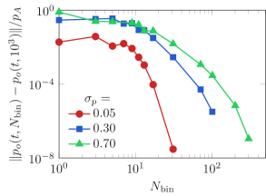
Figure 6: Convergence of ensemble-averaged simulations with $N_{\text{bin}}$ for varying degrees of polydispersity $\sigma_{p}$.

For polydisperse ensemble-averaged simulations, the bubble size distribution, given by a log-normal PDF, must be sampled multiple ($N_{\text{bin}}$) times. Sampling this distribution is expensive, as each sample adds four equations and variables for each grid cell. In figure 6, we show the convergence of bubble-screen-centered pressure with $N_{\text{bin}}$, as compared with a well-resolved $N_{\text{bin}}=10^{3}$ simulation. Convergence appears to be exponential, with generally larger error for larger $\sigma_{p}$ and fixed $N_{\text{bin}}$. This is expected, as larger $\sigma_{p}$ represents a broader bubble size distribution and thus, more samples are required for the same accuracy. Small $N_{\text{bin}}$ entails relatively large error; for $\sigma_{p}=0.3$, $N_{\text{bin}}=11$ gives an error of $8\%$ of $p_{A}$, whereas $N_{\text{bin}}=101$ gives an error of only $10^{-4}\%$. We thus anticipate that, in this case, greater than $N_{\text{bin}}=11$, but less than $N_{\text{bin}}=101$ samples are sufficient for most purposes.

V.5 Computation cost

We compute the computational cost of each method by considering the time-step cost of a simulation configuration. For this benchmarking, simulations were performed with the same three-dimensional grid and matching time-step sizes on a single core of a twelve-core Intel Xeon E5-2670 Haswell $2.3\text{\,}\mathrm{GHz}$ processor. Here, $T_{s}$ is the time-step costs in seconds, which is computed as the average cost of a time-step over 1000 time steps of a single simulation. We emphasize that both methods have the same simulation platform, following the general implementation of Coralic and Colonius (2006), which ensures that the relative costs computed for each method are restricted to the computational bubble model itself.

Figure 7: Time-step cost $T_{s}$ for simulations of varying polydispersity resolution $N_{\text{bin}}$ and initial void fraction $\alpha_{o}$.

Figure 7 shows the relative cost of polydisperse simulations. Polydisperse volume-averaged simulations are no more costly than monodisperse simulations, so $T_{s}$ is independent of $N_{\text{bin}}$. The dashed lines show their cost for different initial void fractions, $\alpha_{o}$, vary because larger $\alpha_{o}$ entails more bubbles, each of which is evolved via the Keller–Miksis equation. For the ensemble-averaged simulations, $T_{s}$ is independent of $\alpha_{o}$, since it is represented as an Eulerian variable on the mesh. Instead, following the previous subsection, the cost is paid when considering polydispersity. Indeed, this cost is significant with $T_{s}$ going as $N_{\text{bin}}$ for $N_{\text{bin}}\gtrsim 10$. Another consideration for the volume-averaged case is that multiple simulations are required for stochastic closure; following figure 5 (a), at least 40 simulations are likely required for most purposes and the dashed lines of figure 7 should be ascended by this factor, accordingly. Thus, for monodisperse simulations, the ensemble-averaging method is cheaper for all $\alpha_{o}$. For the $\alpha_{o}=4\times 10^{-5}$ bubble screen of previous sections, if the bubble population is considered polydisperse with $\sigma_{p}=0.3$ and we accept $1\%$ relative errors in the stochastic closures of both methods, then the methods have nearly the same cost, with ensemble-averaging costing $81\%$ that of volume-averaging. Of course, smaller $\alpha_{o}$ will instead favor volume-averaging.

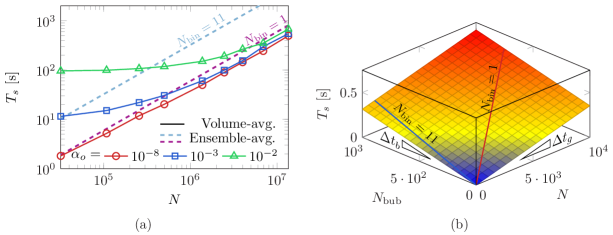
Figure 8: Time-step cost $T_{s}$ for simulations of varying spatial resolution $N=N_{x}N_{y}N_{z}$, polydispersity resolution $N_{\text{bin}}$, and either (a) void fraction $\alpha_{o}$ or (b) number of bubbles $N_{\text{bub}}$ for the volume-averaged simulations.

Our final consideration is the dependence of $T_{s}$ on the spatial grid resolution, and how it couples to the relative costs of polydispersity and number of bubbles $N_{\text{bub}}$, where

$$N_{\text{bub}}=\frac{3\alpha_{o}}{4\pi}\left(\frac{H}{R_{o}}\right)^{3}.$$ (18)

Figure 8 (a) shows this computational cost for several example cases. In the volume-averaged case, $T_{s}$ is linear with $N$ for small $\alpha_{o}$, and plateaus for small $N$ if $\alpha_{o}$ is sufficiently large. This is because increasing $N$ decreases the relative cost of computing the bubble dynamics of volume-averaged simulations, as most of the time is spent reconstructing variables and computing fluxes on the grid. For ensemble-averaged simulations, $T_{s}$ increases linearly with $N$, as the bubble variables are computed in an Eulerian framework. For small $\alpha_{o}=10^{-8}$, the volume-average cost of the bubbles is small, and the ensemble-averaged simulations are more expensive for any $N_{\text{bin}}$. For larger $\alpha_{o}$, the ensemble-average simulations are generally cheaper, except for cases with sufficiently large $N_{\text{bin}}$.

The relative cost of simulating individual bubbles in the volume-averaged case is shown in figure 8 (b). Here, $\Delta t_{b}$ is the additional time-step cost of simulating one additional bubble for fixed $N$, and $\Delta t_{g}$ is this cost for one additional grid point for fixed $N_{\text{bub}}$. We compute $\Delta t_{b}=3.15\times 10^{-4}\,\text{s}/N_{\text{bub}}$ and $\Delta t_{g}=3.53\times 10^{-5}\,\text{s}/N$, and confirm that these values are independent within $1\%$ for varying $N$ and $N_{\text{bub}}$, respectively. From these, the total time-step cost of a volume-averaged simulation is simply $\Delta t=N_{\text{bub}}\Delta t_{b}+N\Delta t_{g}$, which we confirm for independently selected cases is within $2\%$ of the actual cost. In figure 8 (b) we also label the intersection of this curve with the cost of an ensemble-averaged simulation with polydisperse resolution $N_{\text{bin}}$ (which is independent of $N_{\text{bub}}$). Volume-averaged cases with larger $N_{\text{bub}}$ for constant $N_{\text{bin}}$ are more expensive. For example, for $N_{\text{bin}}=11$ and $N=10^{3}$, a single ensemble-averaged simulation is cheaper than a single volume-averaged simulation when $N_{\text{bub}}>916$.

VI Discussion and conclusions

We presented a computational analysis of ensemble- and volume-averaged dilute bubbly flow models in the context of an acoustically excited dilute bubble screen. Results showed, for the first time, that the mixture pressure at the bubble screen center closely matched for both the mean volume-averaged and ensemble-averaged methods.

As a step towards assessing the relative computational cost of each method, we focused on the cost of closing the stochastic part of the models. The volume-averaged numerical model requires multiple, deterministic simulations of heterogeneous, randomized dilute bubble populations to converge to the homogeneous averaged flow. We showed that the error in the mean flow approximation decreased as $\mathcal{O}(N_{\text{sim}}^{-1})$, with the associated coefficient setting the required number of simulations for stochastic closure within a given error bound. In the case of an acoustically excited bubble screen, error in the bubble-screen averaged pressure was about $1\%$ for $N_{\text{sim}}=40$, and independent of the spatial resolution. Polydisperse ensemble-averaged simulations require multiple ($N_{\text{bin}}$) samples of the log-normal PDF of most-probable equilibrium bubble radii. We showed that the error associated with undersampling this PDF decreased approximately exponentially with increasing $N_{\text{bin}}$, with slower decay for larger PDF standard deviations. Ultimately, $N_{\text{bin}}\gtrsim 10$ was required for faithful representation of the polydisperse flow physics. Together, these analyses provided a framework for computing total computational effort.

In the polydisperse case, the cost of ensemble-averaged simulations was dominated by its stochastic closure. That is, the additional reconstructed variables and computed fluxes on the Eulerian grid associated with the underlying PDF were the primary time-cost of simulation for $N_{\text{bin}}>5$. In such cases, ensemble-averaged simulations were generally more expensive than their volume-averaged counterparts. However, monodisperse simulations were generally cheaper for the ensemble-averaged case, as only four additional equations were added to the governing system and no individual bubble dynamics needed to be resolved. These relative costs were complicated by the separate costs of computing single-bubble dynamics and the Euler flow equations in the volume-averaged case. For this, we linearly decomposed these costs such that the relative cost of each method could be assessed for any combination of $N$, $\alpha_{o}$ (or $N_{\text{bub}}$), and $N_{\text{bin}}$. For low void fraction simulations on large spatial grids, the relative cost of computing single-bubble dynamics was small and volume-averaged simulations were preferable. For larger void fractions on relatively coarse meshes, the relative cost of computing the bubble-dynamic equations was large and ensemble-average simulations were preferable.

References

- Reisman et al. (1998) G. E. Reisman, Y.-C. Wang, and C. E. Brennen, J. Fluid Mech. 355, 255 (1998).
- Brennen (1995) C. E. Brennen, Cavitation and bubble dynamics (Oxford University Press, 1995).
- Mettin and Lauterborn (2003) R. Mettin and W. Lauterborn, J. Appl. Mech. Tech. Phys. 44, 17 (2003).
- Risso (2018) F. Risso, Ann. Rev. Fluid Mech. 50, 25 (2018).
- Patek et al. (2004) S. N. Patek, W. L. Korff, and R. Caldwell, Nature 428, 819 (2004).
- Patek and Caldwell (2005) S. Patek and R. Caldwell, J. Exp. Biol. 208, 3655 (2005).
- Bauer (2004) R. T. Bauer, Remarkable shrimps: adaptations and natural history of the carideans, Vol. 7 (University of Oklahoma Press, 2004).
- Koukouvinis et al. (2017) P. Koukouvinis, C. Bruecker, and M. Gavaises, Sci. Rep. 7, 13994 (2017).
- Leighton et al. (2004) T. G. Leighton, S. D. Richards, and P. R. White, in Acoustics Bulletin, Vol. 29 (2004) pp. 24–29.
- Leighton et al. (2007) T. G. Leighton, D. Finfer, E. Grover, and P. R. White, in Acoustics Bulletin, Vol. 22 (2007) pp. 17–21.
- Pickard (1981) W. Pickard, Prog. Biophy. Molec. Biol. 37, 181 (1981).
- Coleman et al. (1987) A. J. Coleman, J. E. Saunders, L. Crum, and M. Dyson, Ultrasound Med. Biol. 13, 69 (1987).
- Pishchalnikov et al. (2003) Y. A. Pishchalnikov, O. A. Sapozhnikov, M. R. Bailey, J. C. Williams, R. O. Cleveland, T. Colonius, L. A. Crum, A. P. Evan, and J. A. McAteer, J. Endourol. 17, 435 (2003).
- Ikeda et al. (2006) T. Ikeda, S. Yoshizawa, T. Masakata, J. S. Allen, S. Takagi, N. Ohta, T. Kitamura, and Y. Matsumoto, Ultrasound Med. Biol. 32, 1383 (2006).
- Surov (1999) V. Surov, Tech. Phys. 44, 37 (1999).
- Etter (2013) P. C. Etter, Underwater acoustic modeling and simulation (CRC Press, 2013).
- Kedrinskii (1976) V. Kedrinskii, Acta Astro. 3, 623 (1976).
- Weyler et al. (1971) M. Weyler, V. Streeter, and P. Larsen, J. Basic Eng. 93, 1 (1971).
- Streeter (1983) V. Streeter, J. Hydraulic Eng. 109, 1407 (1983).
- Naudé and Ellis (1961) F. Naudé and A. Ellis, J. Basic Eng. 83, 648 (1961).
- Sharma et al. (1990) S. Sharma, K. Mani, and V. Arakeri, J. Sound Vib. 138, 255 (1990).
- Ji et al. (2012) B. Ji, X. Luo, X. Peng, Y. Wu, and H. Xu, Int. J. Mult. Flow 43, 13 (2012).
- d’Agostino and Brennen (1983) L. d’Agostino and C. E. Brennen, in Cavitation and Multiphase Flow Forum, Vol. 2 (American Society of Mechanical Engineers, 1983) pp. 72–75.
- Foldy (1945) L. L. Foldy, Phys. Rev. 67, 107 (1945).
- Iordanskii (1960) S. V. Iordanskii, Zh. Prikl. Mekh. Tekhn. Fiz. 3, 102 (1960).
- Kogarko (1964) B. S. Kogarko, Dokl. Akad. Nauk SSSR 115, 779 (1964).
- Wijngaarden (1964) L. V. Wijngaarden, in 11th Int. Cong. Appl. Mech (1964) pp. 854–861.
- Wijngaarden (1968) L. V. Wijngaarden, J. Fluid Mech. 33, 465 (1968).
- Zhang and Prosperetti (1994) D. Z. Zhang and A. Prosperetti, Phys. Fluids 6 (1994).
- Commander and Prosperetti (1989) K. W. Commander and A. Prosperetti, J. Acoustic. Soc. Am. 85 (1989).
- Fuster and Colonius (2011) D. Fuster and T. Colonius, J. Fluid Mech. 688, 352 (2011).
- Ando et al. (2011) K. Ando, T. Colonius, and C. E. Brennen, Int. J. Mult. Flow 37, 596 (2011).
- Nigmatulin (1979) R. I. Nigmatulin, Int. J. Heat Mass Transfer 5, 353 (1979).
- Prosperetti (2001) A. Prosperetti, in Handbook of Elastic Properties of Solids, Liquids, and Gases, Vol. 4, edited by M. Levy, H. E. Bass, and R. Stern (Academic Press, 2001).
- Batchelor (1970) G. K. Batchelor, J. Fluid Mech. 41, 545 (1970).
- Biesheuvel and Wijngaarden (1984) A. Biesheuvel and L. V. Wijngaarden, J. Fluid Mech. 148, 301 (1984).
- Matsumoto and Kameda (1996) Y. Matsumoto and M. Kameda, JSME Int. J. Ser. B 39, 264 (1996).
- Colonius et al. (2008) T. Colonius, R. Hagmeijer, K. Ando, and C. E. Brennen, Phys. Fluids 20 (2008).
- Ando (2010) K. Ando, Effects of polydispersity in bubbly flows, Ph.D. thesis, California Institute of Technology (2010).
- Menikoff and Plohr (1989) R. Menikoff and B. J. Plohr, Rev. Mod. Phys. 61, 75 (1989).
- Maeda and Colonius (2018) K. Maeda and T. Colonius, J. Comp. Phys. 371, 994 (2018).
- Keller and Miksis (1980) J. B. Keller and M. Miksis, J. Acoustic. Soc. Am. 68 (1980).
- Preston et al. (2007) A. Preston, T. Colonius, and C. E. Brennen, Phys. Fluids 19 (2007).
- Coralic and Colonius (2006) V. Coralic and T. Colonius, J. Comp. Phys. 219, 715 (2006).
- Toro et al. (1994) E. Toro, M. Spruce, and W. Speares, Shock waves 4, 25 (1994).
- Gottlieb and Shu (1998) S. Gottlieb and C.-W. Shu, Math. Comput. 67, 73 (1998).
- Langefors and Kihlström (1967) U. Langefors and B. Kihlström, The modern technique of rock blasting (New York, John Wiley & Sons, 1967).
- Domenico (1982) S. N. Domenico, Geophysics 47, 345 (1982).
- Blackaert et al. (2008) K. Blackaert, F. A. Buschman, R. Schielen, and J. H. A. Wijbenga, J. Hydraulic Eng. 134, 184 (2008).
- Patrick et al. (1985) P. H. Patrick, A. Christie, D. Sager, C. Hocutt, and J. Stauffer, Fish. Res. 3, 157 (1985).