Measurement of telescope transmission using a Collimated Beam Projector

Abstract

With the increasingly large number of type Ia supernova being detected by current-generation survey telescopes, and even more expected with the upcoming Rubin Observatory Legacy Survey of Space and Time, the precision of cosmological measurements will become limited by systematic uncertainties in flux calibration rather than statistical noise. One major source of systematic error in determining SNe Ia color evolution (needed for distance estimation) is uncertainty in telescope transmission, both within and between surveys. We introduce here the Collimated Beam Projector (CBP), which is meant to measure a telescope transmission with collimated light. The collimated beam more closely mimics a stellar wavefront as compared to flat-field based instruments, allowing for more precise handling of systematic errors such as those from ghosting and filter angle-of-incidence dependence. As a proof of concept, we present CBP measurements of the StarDICE prototype telescope, achieving a standard ($1\sigma$) uncertainty of $3$ % on average over the full wavelength range measured with a single beam illumination.

*Nicholas Mondrik, nmondrik@gmail.com

1 Introduction

Multi-band photometry permits measurements of much fainter sources than spectroscopy while still preserving low spectral resolution components of the observed SED (spectral energy distribution). In general, there is a large number of desirable photometric measurements that are useful to astronomers, including, but not limited to: top-of-atmosphere (TOA) flux, flux corrected for Galactic extinction, and flux corrected for both Galactic and host-galaxy extinction, for supernova (SNe) cosmology in particular[1, 2]. Only instrumental magnitudes are directly measured, and include contributions from telescope transmission idiosyncrasies and atmospheric transmission variations that serve to obscure astrophysically interesting features[3].

Knowledge of instrumental passbands is particularly useful when attempting to determine magnitudes of sources having SEDs that are dissimilar to standard flux calibration stars, as in the case of SNe Ia cosmology. With the advent of large-scale transient surveys such as Rubin Legacy Survey of Space and Time[4, 5] (LSST) undertaken by Rubin Observatory, the number of Type Ia supernovae will be large enough that systematic calibration uncertainty will become the limiting factor in the determination of cosmological parameters[6]. Additionally, state of the art survey calibration schemes, such as the Forward Global Calibration Method[7], can take passband measurements as inputs, thereby increasing the accuracy and precision of survey measurements by accounting for the variations in the spectra of field stars.

The goal of photometric calibration is to arrive at a measure of brightness that is an accurate measurement of the source SED integrated over a given bandpass and that accounts for temporal variations in the atmospheric and optical transmission functions. The material presented here is focused on the problem of determining the optical transmission function of the telescope, but an overview of factors impacting photometric calibration of surveys can be found in Ref. 8. By optical transmission function, we mean the fraction of photons that enter the telescope, are converted to photo-electrons, and subsequently read out of the CCD (charge-coupled device). The simplest method of measuring this quantity would then be to send a known number of photons down the telescope’s optics, and compare the number measured on the CCD to the number originally emitted.

The usual way to accomplish this mapping in astronomy is by tying back to almost pure hydrogen white dwarfs stars, for which we believe we are able to estimate the flux based on spectral line measurements and radiative transfer calculations [9]. Tying to standards that can actually be built on Earth has also been tried, either by creating a proxy of a black body that can be directly observed by the telescope [10], or by creating a calibrated stable light source using a calibrated detector, usually a photodiode provided by the National Institute of Standards and Technology (NIST)[3]. While this latter approach relies on a metrology chain with more intermediate steps, it capitalizes on the fact that NIST photodiode’s quantum efficiency (QE) can be calibrated with an uncertainty on the order of $0.1\%$ over the full optical range (400nm-1000nm).

This is the approach we choose for the Collimated Beam Projector: By using a NIST-calibrated photodiode to normalize away the variations in the calibration light source, we are seeking to transfer a known flux scale, such as the one defined by the Primary Optical Watt Radiometer[11] (POWR) at NIST, onto a telescope CCD which can then transfer that calibration to an astrophysical source. Technically speaking, POWR provides an optical-watt power scale, which is distinct from a flux scale by a factor of area (Flux $\equiv$ Power/Area). Because we are interested here only in chromatic variations, and not absolute calibration, we may treat the two as equivalent. Although an absolute flux scale is desirable (transmission of the system is known exactly at all wavelengths), in many practical cases a relative flux scale is sufficient. By relative flux scale, we mean that the transmission ratio $T(\lambda)/T(\lambda^{\prime})$ is known between any two generic wavelengths, but the overall grayscale normalization is unknown. Said more simply, we need to ensure that there are no temporal or spatial (over the detector) variations in observed ratios of fluxes (colors), and that these ratios are consistent with the true flux ratios.

1.1 Extant transmission measurement devices

Astronomers have wrangled with the challenges of calibrating CCD-based observations since the advent of the devices in the late 20^th century. Bias frames, flat field exposures, star flats, and many other types of data are frequently used by astronomers to contend with the temporal and spatial non-uniformity of telescope optical systems. The flat field is of particular interest to the challenge of determining instrumental passbands because it is an attempt to standardize the response of each pixel in a telescope system. A typical flat field system uses a white-light source to illuminate a lambertian reflecting screen, usually far out-of-focus, which is observed by the telescope, with the end result being a “flat” (constant surface brightness) image on the detector. The flat field obtained, which has different scattered and stray light behavior than a start field science beam, generally tends to homogenize variability arising from the screen construction, and is used to normalize away pixel-to-pixel variations in images of astrophysical sources.

However, as has been pointed out (e.g., Refs. 12, 13), naive application of flat fields may introduce systematic errors that limit the ultimate uncertainty of the measurement. A flat field may not perfectly mimic the response to astronomical sources due to several factors such as delineating the difference between variations in pixel size, caused by departure from a rectilinear grid (due, for example, to lateral electric fields within the sensor that distort pixel gridlines) from true variations in pixel QE. One of the fundamental issues with conflating these two processes is that variations in pixel size are flux-conserving (although a given photo-electron may end up in a neighboring pixel, it is still present and can be counted), while variations in QE are not (the photo-electron is never generated in the first place).

The sheer ubiquity of flat field screens at observatories does however, make them a tantalizing component to leverage in the challenge of measuring telescope throughputs. It remains then, to concoct a scheme by which variations in pixel size can be decoupled from variations in QE. One method is to use tunable, narrowband light to illuminate a flat field screen, generating a data cube of flats at each wavelength over the spectral range of interest. By looking at the signal variation of each pixel with wavelength, one can remain agnostic to the average size of the pixel. We stress average, because the method is still sensitive to the wavelength-dependent component of pixel size variations. As an example, in the presence of a static lateral electric field (for example, from impurity gradients), a photo-electron from a blue photon, which converts near the back surface of the CCD, will experience greater deflection than a red photon, which converts deeper in the device. This would make the pixel in question appear less responsive in the blue than the red, and again the flux-conserving pixel size variations can be mistaken for QE variation. Overall, this type of method reduces confusion between pixel size and QE, becoming instead limited by the wavelength-derivative of pixel size variations. More appropriately, they might be said to be limited by the differential size-derivative of pixels, since leakage of photo-electrons out of a pixel can be compensated for by leakage into the pixel from its neighbors.

Several experiments and devices have been constructed along these lines, for example, the method proposed in Ref. 3 and implemented in Ref. 14 used a photodiode-monitored, monochromatic, tunable laser source reflected off of a flat field screen to measure the transmission function of the PanSTARRS telescope. The DECal system[15, 16] on the Cerro Tololo Inter-American Observatory’s Blanco telescope, similarly illuminates a flat field screen with a combination of LEDs and a white-light powered monochromator, which is monitored by a photodiode.

Challenges remain for flat-field based systems, however. In particular, there are systematic differences in scattered light paths between flat field and stellar illumination patterns. These differences would result in systematic errors when deriving transmission measurements for point sources. It would be ideal, then, to illuminate the telescope with a wavefront similar to that of a star: i.e., full-pupil and planar. This would effectively side-step the challenging task of deriving corrections for point-source images from surface-brightness based flats.

The SCALA system[17] on the University of Hawaii 88-inch Telescope uses a white-light powered monochromator as its illumination source, which is fed into a series of integrating spheres attached to a frame mounted on the interior of the telescope dome. Apertures on the outputs of the integrating spheres are collimated by mirrors and re-imaged onto the focal plane of the SuperNova Integral Field Spectrograph (SNIFS). Two of the collimated beams is monitored by a Cooled Large Area Photodiode[18], which provides normalization. In this case, full pupil illumination is traded off against using a collimated beam re-imaging system to project large (1^∘) spots onto the focal plane. Tying the calibration of SNIFS to the NIST definition of the optical Watt in turn permits the SNfactory to provide, by repeated observations of standard stars over more than a decade, a well calibrated star network covering a large fraction of the sky observable from Hawaii[19].

The NIST Stars project uses a spectrograph to observe a NIST-calibrated light source and standard stars alternately, thereby transferring the light source calibration to the standard stars. When the light source is placed sufficiently far away, the wavefront is effectively parallel when entering the telescope, thus generating a full-pupil collimated beam.

The StarDICE project is of the same flavor, but uses a stable calibrated poly-chromatic source made of LEDs placed at $\sim 200$ m from a $\sim 1$ m focal length telescope as an artificial star. It aims at providing a network of stars of magnitude between 10 and 13 calibrated with traceability to the SI (Système International d’Unités) through the NIST POWR scale by observing in turn the artificial star and the CALSPEC stars. This procedure makes the measurement of the transmission of the StarDICE telescope mandatory.

In this paper, we present the Collimated Beam Projector (CBP) instrument, a telescope throughput measurement system[20, 21, 22]. In Sec. 2, we explore design considerations in general, and in Sec. 3 we describe the design and components of our CBP system in particular. Section 4 outlines the method for tying CBP measurements back to the flux scale established at NIST, Sec. 5 describes the StarDICE experiment and CBP setup, and Sec. 6 describes the data reduction procedure. Section 7 presents transmission curves for the StarDICE prototype telescope, taken at the Laboratoire de Physique Nucléaire et des Hautes Énergies (LPNHE), and presents lessons learned during this phase. Finally Sec. 8 reviews planned upgrades and revisions to the system.

2 Design Considerations for Optical Transmission Measurement

To design an instrument to measure the optical throughput of an imaging system, we must first understand both the optical properties and measurement goals of the system. Using $t$ for time, $\lambda$ for wavelength, $\mathbf{x}$ for the vector position, $\boldsymbol{\gamma}$ for a given altitude and azimuth, and $\mathbf{r}$ the location on the primary mirror, the flux arriving from a given source on the focal plane, $\phi(t,\mathbf{x},\boldsymbol{\gamma})$, can be expressed as

$$\phi(t,\mathbf{x},\gamma)=C(t)\int A(t,\lambda,\boldsymbol{\gamma})\,T(t,\lambda,\mathbf{x},\mathbf{r},\boldsymbol{\alpha})\,S(t,\lambda,\boldsymbol{\alpha})\,d\lambda\,d^{2}\boldsymbol{\alpha}\,d^{2}\mathbf{r},$$ (1)

where $C(t)$ is a constant with respect to focal plane position, telescope pointing, and wavelength (e.g., collecting area, electronic gain), $A(t,\lambda,\boldsymbol{\gamma})$ is the instantaneous atmospheric transmission function, $T(t,\lambda,\textbf{x},\textbf{r},\boldsymbol{\alpha})$ is the instrumental transmission function, and $S(t,\lambda,\boldsymbol{\alpha})$ is the total TOA photon flux incident on the primary from sources at angle $\boldsymbol{\alpha}$ relative to the pointing of the telescope. The integrals are over all wavelengths, relative angles, and the entirety of the primary, respectively.

To measure the transmission of a telescope, we must contend with all of the terms above, with a few modifications. Relative to standard astronomical measurements, $A$ is much suppressed due to shorter path-lengths and $S$ is instead the spectrum of the calibration light. Our ultimate goal is to estimate $T$, the transmission function of the telescope imposed on astrophysical point-source wavefronts. Armed with this expression, we can begin to explore the design requirements for our transmission measurement systems.

2.1 Motivation for using collimated beams

A planar wavefront incident on the primary at a defined angle $\boldsymbol{\alpha}$ has a fixed ghosting pattern as a function of wavelength set by the geometry of a given optical system. When a telescope is illuminated with a non-planar wavefront, ghosts and other scattered light are superimposed on the target region, resulting in a subtly different transmission function than the one experienced by an astrophysical source. For this reason, flat fields, which illuminate the telescope at all angles, are not ideal calibrators for point sources.

Beyond the angle of incidence, the location of a photon’s impact on the telescope primary, $\mathbf{r}$, can play a major role in transmission measurements, particularly for interference filter-based systems that are not designed with variable multi-layer coating thicknesses to account for geometrically-related shifts in bandpasses. For these systems, the incidence angle $\theta$ at which the light passes through the filter changes the effective transmission of the filter. An approximation of the shift in transmission for a filter for a given incidence angle $\theta$ and index of refraction $n$ is[23]

$$T(\lambda,\,\theta)=T\Big{(}\lambda\,(1-\frac{\sin^{2}{\theta}}{n^{2}})^{-\frac{1}{2}},\,\theta=0\Big{)}.$$ (2)

where we see that the effect is essentially a blueshift of the filter transmission at $\theta=0$.

If the wavefront injected into the telescope is non-planar, there will be a difference in the measured filter transmission and transmission function experienced by a star, the scope of which is dependent on telescope geometry (in particular, the measured filter passband will be broadened according to the above equation, weighted by the relative photon flux density at each angle $\theta$).

The location of filter edges is of particular concern, so it is worth understanding their impact on transmission measurement devices. Photons with a wavelength located within an edge are highly likely to experience internal reflection within the filter because the transmission significantly deviates from unity and from zero, by definition. These internal reflections can escape the filter and land on the detector, contributing significantly to scattered light. For a collimated system, there is some hope that these scattering patterns approximate (to a degree) that of a stellar wavefront. For a flat field system, whose photon phase-space distribution is different than that of a plane wave illumination (with a single phase and direction), there is additional systematic uncertainty.

Together, these two concerns motivate the use of collimated light, rather than flat fields. It is important to note that here we have assumed that the goal of the survey is to measure point sources – if measurements of surface brightness are required, then projecting a planar wavefront onto the telescope is not a requirement anymore, and flat-field based methods are more appropriate.

2.2 Light source requirements

A first requirement is based on the tautology that the light source used to measure the transmission function must be capable of emitting light over the entire wavelength range of interest (roughly 300 nm - 1100 nm for optical systems). Assuming negligible attenuation from atmospheric effects ($A$ is small in setups where the light source is close to the telescope), the relevant wavelength-dependent transmission variations to be measured are those in $T$. This motivates an additional property of the light source: that the optical bandwidth should be small compared to variations expected in $T$. For interference filter based systems, this scale is set naturally by the filter edges, which transition from opaque to transparent over roughly a 20 nm span. This results in a filter transmission change ratio of around 1% per $0.2$ nm. Properly sampling smoothly if rapidly varying filter edges at the percent level therefore suggests optical bandwidths of order 1 nm, which is readily achievable by devices such as monochromators and tunable lasers. In addition to the wavelength requirement, the output flux of the light source, $S$, must be known at the sub-percent level.

3 Design of the Collimated Beam Projector (CBP)

We present here an overview of the CBP system; see Refs. 20, 21 for additional details on CBP design.

The CBP consists of two components: an imaging system and a light source. A tunable laser (with associated coupling optics) provides high-power, narrowband light for the CBP imaging system. The imaging system is composed of a collimating optic, a focal plane mask, and an integrating sphere, with a fiber optic cable connecting the output of the laser to the integrating sphere. This system is then attached to an alt-az mount that allows the CBP to be pointed remotely. By coordinating the alt-az pointing of the CBP and the telescope, it is possible to point the CBP beam at a different section of the primary while leaving the position on the detector fixed. This process, which we dub “pupil stitching”, allows the CBP to scan the full primary mirror (and by extension, the different paths taken by photons en route to the same detector pixels). This in theory enables a synthetic full-pupil measurement with a collimated beam (essentially emulating a stellar wavefront). Given hard time constraints in particular due to the limited availability of the laser at LPNHE, we defer the full pupil measurement to a forthcoming paper (Souverin et al. in prep.).

Taking the constraints imposed above and re-writing Eqn. 1 for an input photon distribution provided a single CBP pointing, we obtain

$$\phi_{\mathrm{CBP}}(t,\textbf{x},\lambda)=C(t)\int_{\mathrm{CBP}}T(t,\lambda,\textbf{x},\textbf{r},\boldsymbol{\alpha})\,S(t,\lambda,\boldsymbol{\alpha})\,d^{2}\textbf{r},$$ (3)

where the integral is over the CBP’s footprint on the primary, and we have assumed the CBP’s output flux $S(t,\lambda,\boldsymbol{\alpha})$ can be described as $S(t,\lambda^{\prime},\boldsymbol{\alpha^{\prime}})\,\delta(\lambda^{\prime}-\lambda)\,\delta(\boldsymbol{\alpha}^{\prime}-\boldsymbol{\alpha})$, i.e. the CBP output is monochromatic with a well-defined angle relative to the telescope (indicated by the Dirac delta functions $\delta(\dots)$), and that atmospheric attenuation is negligible. In the case where the CBP’s footprint is small relative to the primary, one can additionally multiply by another factor of $\delta(\textbf{r}^{\prime}-\textbf{r})$, and assume that the measurement is a point-like sampling of the primary. Alternatively, one might make the assertion that the system’s optical transmission is not a strong function of the input beam’s location on the primary, and thereby absorb the (now constant) integral into $C(t)$. In all generality, this latter assertion is untrue since different input beam locations on the primary result usually in different angles of the converging beam passing through an interference filter before hitting the detector, though the level of deviation is dependent on telescope geometry and is generally smaller for slower optical systems, which operate at smaller angles.

This assumption leaves for a later work (Souverin et al. in prep) the discussion about the fact that different areas on a primary mirror can have very different reflectivity properties. The actual measurement of this variability will be part of the strategy developped in forthcomming papers (StarDICE collaboration 2023-2024) in order to reconstruct the full pupil transmission from CBP patch measurements.

3.1 Tunable Laser

The light source for the CBP is an EKSPLA NT-242 tunable laser, which outputs 3 ns to 6 ns laser pulses at a 1 kHz repetition rate, with a total output power of 0.5 W at roughly 450 nm. The tunable laser uses a non-linear optical process (spontaneous parametric down-conversion, SPDC) inside of a crystal (called an optical parametric oscillator, or OPO) to convert an incident photon of frequency $\nu_{1}$ (the OPO pump beam) into two photons such that $\nu_{1}=\nu_{2}+\nu_{3}$, where energy and momentum remain conserved. In the case of the NT-242, these two photons are cross-polarized (formally, this means the process is type-II SPDC), which allows for separation of the “signal” and “idler” beams (the high- and low-frequency output beams, respectively) via a Rochon prism within the laser. In the case of the NT-242 laser used here, the pump beam is provided by a Nd:YAG laser at 1064 nm. This pump beam is tripled in frequency to 355 nm before reaching the OPO, meaning the OPO itself is pumped by a 355 nm beam, which allows access to wavelengths above 355 nm. In order to reach wavelengths below the OPO pump wavelength, the beam is sent through a second harmonic generator (SHG), which doubles the frequency of the incoming light. The SHG allows access to wavelengths below 355 nm, at the cost of much-reduced efficiency. In the end, the NT-242 laser is tunable from below 300 nm to over 2 $\mu$m, which is well matched to the sensitivity range of CCDs. The tunable laser provides high flux in a narrow bandpass, $\lesssim 5$ cm^-1, which corresponds to approximately $\delta\lambda=0.13$ nm at 500 nm, and $\delta\lambda=0.5$ nm at 1 $\mu$m. These are upper limits quoted by the manufacturer, and measurements taken using these systems show bandwidths of 0.08 nm to 0.48 nm between 350 nm and 1100 nm[24]. As these bandpasses are small compared to the accuracy achieved at this stage, we treat the output of the laser as monochromatic.

There are additional concerns that must be addressed when using tunable lasers, and we present here the major challenges; for an overview of tunable lasers in optical calibration applications, see Ref. 24. There are three primary obstacles to overcome: excessive brightness in some regions, low efficiency near the degeneracy point of the system, and incomplete separation of the signal and idler beams in the degeneracy region (around 710 nm for the EKSPLA NT-242). To address brightness concerns, we added a reflective neutral density (ND) filter to the fiber coupling system so that the beam can be attenuated. The degeneracy region occurs when $\nu_{\mathrm{signal}}\simeq\nu_{\mathrm{idler}}\simeq\nu_{\mathrm{pump}}/2$, and is characterized by low output power and poor separation of the signal and idler beams. Low efficiency in the degnereracy region can be overcome either by increasing integration times, or by using a different light source. For example, an OPO pumped at 532 nm would have its degeneracy point at 1064 nm, in a part of the spectrum farther from filter edges. Enhanced separation of the signal and idler beams can be achieved in several ways, for example, with the addition of rotating polarizers or short-/long-pass filters with cut-off/-on wavelengths equal to the OPO pump beam wavelength. Such optical elements are not present in our current fiber coupling scheme, but will be installed for our next iteration.

The light first passes through a flip mirror, which optionally steers the beam into a beam dump, shuttering the laser. Afterwards, the beam passes through a variable ND filter mounted on a rotation stage. This filter allows for attenuation of the beam in regions where the laser is so bright as to require sub-second exposure times. The beam then is coupled into a reflective fiber collimator, which is connected to the integrating sphere via an optical fiber. Figure 2 summarizes this setup.

3.2 CBP imaging system

The CBP imaging system is comprised of a Sonnar^® CFE Superachromat 5.6/250 mm lens, which images a mask held by a Finger Lakes Instrumentation (FLI) CL1-10 filter wheel backlit by a Labsphere integrating sphere. The lens’ focus is not strongly chromatic, which should allow us to forgo re-focusing the CBP optics at each wavelength. The FLI filter wheel contains two internal wheels; one holds the masks to be re-imaged, and another holds an f-stop aperture, which prevents injection of light at angles too extreme to be focused by the lens. The CBP currently holds 3 imaging masks: a 20 $\mu$m pinhole, a 5x5 grid of 20 $\mu$m pinholes at 200 $\mu$m spacing, and a large 500 $\mu$m pinhole. The single 20 $\mu$m allows for precise determination of ghost locations without confusion from nearby pinholes, while the pinhole grid allows for multiplexing of transmission measurements as a function of sensor location. Using the CBP with no pinhole allows for coarse alignment of the CBP and telescope, while the 500 $\mu$m pinhole is useful in achieving fine alignment and for providing a resolved, locally flat region on the detector. The 500 $\mu$m pinhole is also required for calibrating the CBP, as the smaller pinholes do not provide sufficient brightness. It should be noted that such small pinholes tend to have large variations in their diameters, and the manufacturer of the masks used here, Lenox Laser, quotes $\pm 10$ % tolerance on the diameter, which implies variations in pinhole area of up to 50 % in the worst-case scenario.

In addition to the output port and light injection port, there are two devices attached to the integrating sphere. The first is the monitor photodiode, a Thorlabs SM1PD2A, which normalizes away temporal variations in laser power. The photodiode is connected to a Keithley 6514 charge-integrating electrometer, which measures the amount of charge collected by the photodiode during an exposure. Because there is a saturation limit to the collection capacity of the electrometer’s measurement capacitor, an aperture of 1 mm is placed in front of the photodiode, allowing for use of integration times commensurate with those needed for telescope measurements. The second device connected to the integrating sphere is an Ocean Optics QE65000 fiber-fed universal serial bus spectrograph, which monitors the wavelength emitted by the laser. The integrating sphere itself is necessary to ensure that all pinholes are illuminated homogenously and achromatically with respect to the spectrograph and the monitoring photodiode, since we cannot monitor the flux emitted by each individual pinhole. If the surface brightness seen by the pinhole grid varied with wavelength across the grid, it would imprint itself as a focal plane transmission gradient on the telescope. The integrating sphere also ensures that the light seen by the monitoring equipment (photodiode, spectrograph) has the same surface brightness as the light illuminating the pinhole grid. It has to be noted that these desirable features come at the price of decreasing the surface brightness of the pinholes in direct proportion of the size of the integrating sphere used. In the current design, the integrating sphere diameter (6 inches) has been fixed by the desire to multiplex the transmission measurement using a grid of multiple pinholes. This in turn resulted in a large flux dillution that required such a powerful light source as the laser.

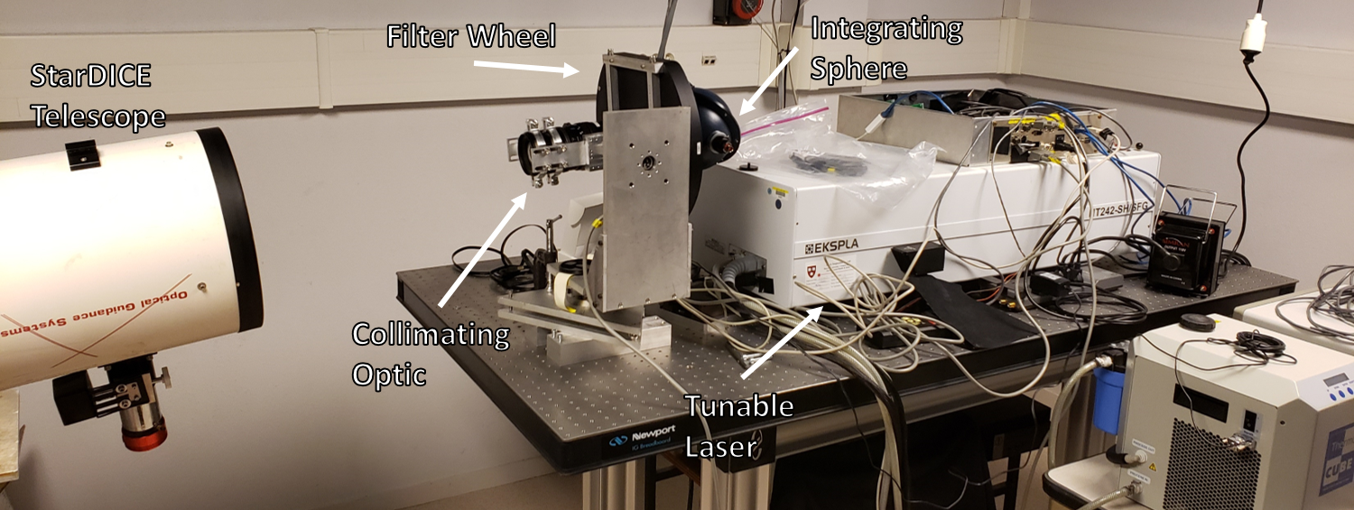
Figure 1: An image of the CBP installed in the StarDICE lab at LPNHE.

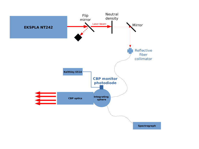
Figure 2: Schematic of the CBP light injection. The telescope measured is placed in front of the CBP optics.

4 Establishing the CBP flux scale

In order to transfer the detector-based flux scale established at NIST to the CBP, the CBP optics were sent to NIST to be calibrated against one of the trap detectors used to hold the POWR optical watt scale. This step is necessary because the CBP input flux is monitored inside the integrating sphere, but the light must pass through an additional strongly chromatic element (the collimating lens) prior to entering the telescope. It is therefore necessary to have an additional calibration at each wavelength of interest between the integrating sphere flux measured by the CBP monitoring photodiode and the actual light emitted by the system.

This calibration took place in three steps. An overview of the calibration process is shown in Fig. 3. The reason why the CBP was not directly calibrated using the calibrated photodiode is because the calibrated photodiode alone is too small to sample the entire CBP output beam, and had poor signal-to-noise when only subsampling the beam. A different calibration scheme, using larger solar cells tied to the NIST optical watt definition[25] is currently being implemented and will be presented in a forthcoming publication (Souverin et al. in prep.).

During all steps, all optics and photodiodes were in a light-tight box, and the laser was coupled into the box through a fiber-optic cable. During each step of measurement, the laser was tuned automatically across the spectral range for calibration. Because the laser delivers light pulses of $\sim 10~{}ns$ at a frequency of 1 kHz, we choose to operate the Keithley 6514 in charge accumulation mode. For this mode of operation, a computer-controlled shutter at the laser output limits the exposure time (typically 1 sec.) of the laser to the fiber. The two photodiodes (the CBP monitor photodiode and the calibrated photodiode, see below) were connected to a separate charge accumulation electrometer, and both electrometers started charge accumulation just before the opening of the laser shutter and stopped accumulation just after closing of the laser shutter. Subsequently, the total amount of accumulated charge, in Coulombs, was read out from each electrometer.

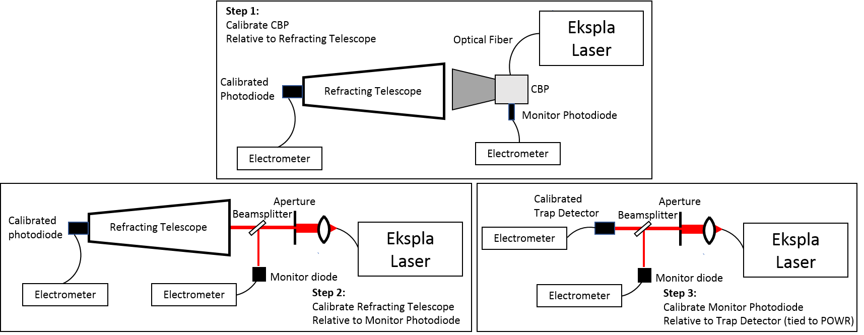
Figure 3: A schematic illustrating the three-step process used to transfer the POWR-traceable calibration of a NIST trap detector to the CBP. Step 1 measures the ratio $Q_{\mathrm{CBP}}/Q_{\mathrm{Telescope}}$ measured respectively by the CBP monitor photodiode and the NIST calibrated photodiode. Likewise the ratios $Q_{\mathrm{Telescope}}/Q_{\mathrm{Monitor}}$ and $Q_{\mathrm{Monitor}}/Q_{\mathrm{Trap}}$ for steps 2 and 3 are obtained by comparing the measurements of the Monitor diode with the NIST calibrated photodiode and the Calibrated Trap detector respectively. The product of the ratios, multiplied by the responsivity of the trap detector, gives the responsivity of the CBP in units of [A W^-1]. The inverse of the CBP responsivity is defined to be the CBP calibration factor. The calibrated photodiode refered to in step 1 and 2 is a NIST-calibrated photodiode with respect to POWR.

In step 1, the CBP illuminated the entrance pupil of a 100 mm diameter refracting telescope with a NIST-calibrated photodiode (referred to as the “calibrated photodiode” in the following and in step 1 and 2 of Fig. 3) at its focus. The focused beam underfilled the calibrated photodiode, ensuring the full collection of the incoming beam. The charge $Q_{\mathrm{CBP}}$ on the CBP monitor photodiode, and the charge $Q_{\mathrm{Telescope}}$ on the calibrated photodiode, were read out after one laser exposure cycle at each wavelength. The ratio $Q_{\mathrm{CBP}}/Q_{\mathrm{Telescope}}$ then references the CBP photodiode to the calibrated photodiode. Data for this step, plotted as $Q_{\mathrm{Telescope}}/Q_{\mathrm{CBP}}$, is shown in Fig. 4a.

The next two steps reference the calibrated photodiode to the POWR-calibrated trap detector through an intermediate monitor photodiode. The trap detector used here is a 3-element arrangement of photodiodes such that a plane-parallel beam of incoming light must make 5 reflections before escaping, boosting the effective quantum efficiency of the trap relative to a single photodiode. These two steps use a different fiber optic cable than the first step, and the fiber optic transmitting the laser light was passed through a speckle reducer that modulated a section of the fiber at high frequency to mix the modes. Within the light-tight box, the fiber output port was placed at the focus of a 100 mm, f/2.8 refractive collimator. The resulting collimated beam was passed first through an aperture to reduce its diameter to 5 mm, then through a beamsplitter with an intermediate monitor photodiode (10 mm x 10 mm called monitor diode in Fig. 4a-c) set to capture the reflected beam.

For step 2, the beam transmitted through the beamsplitter illuminated the refracting telescope with the calibrated photodiode at its focus. The charge $Q_{\mathrm{Telescope}}$ on the calibrated photodiode and the charge $Q_{\mathrm{Monitor}}$ on the intermediate monitor photodiode were read out at each wavelength, so the ratio $Q_{\mathrm{Telescope}}/Q_{\mathrm{Monitor}}$ references the calibrated photodiode to the intermediate monitor.

For the step 3, the beam transmitted through the beamsplitter illuminated and completely underfilled the trap detector. The charge $Q_{\mathrm{Monitor}}$ on the intermediate monitor photodiode and the charge $Q_{\mathrm{Trap}}$ references the intermediate monitor to the trap. Data for the combined results of these two steps are plotted as $Q_{\mathrm{Telescope}}/Q_{\mathrm{Trap}}$ in Fig. 4b.

We therefore measure at each wavelength, three charge ratios: $Q_{\mathrm{CBP}}/Q_{\mathrm{Telescope}}$, $Q_{\mathrm{Telescope}}/Q_{\mathrm{Monitor}}$, and $Q_{\mathrm{Monitor}}/Q_{\mathrm{Trap}}$, each ratio corresponding to one of the three measurements steps. The product of these gives $Q_{\mathrm{CBP}}/Q_{\mathrm{Trap}}$,

$$\frac{Q_{\mathrm{CBP}}}{Q_{\mathrm{Trap}}}=\frac{Q_{\mathrm{CBP}}}{Q_{\mathrm{Telescope}}}\frac{Q_{\mathrm{Telescope}}}{Q_{\mathrm{Monitor}}}\frac{Q_{\mathrm{Monitor}}}{Q_{\mathrm{Trap}}}$$ (4)

The CBP calibration factor $T_{\mathrm{CBP}}(\lambda)$, defined at each wavelength as the number of photons out of the CBP per number of photoelectrons measured by the CBP monitor photodiode, is thus given by:

$$T_{\mathrm{CBP}}(\lambda)=\frac{Q_{\mathrm{Trap}}}{Q_{\mathrm{CBP}}}\frac{1}{EQE_{\mathrm{Trap}}}$$ (5)

where $EQE_{\mathrm{Trap}}$ is the external quantum efficiency of the trap detector at each wavelength as calibrated by POWR. The resulting calibration factor is plotted in Fig.4c.

Since this paper aims at demonstrating the ability of a CBP to measure the chromatic variations of telescope and filter transmissions, we don’t keep track of the absolute grey scale but only of $T_{\mathrm{CBP}}$ up to an arbitrary grey scale, without propagating the ratios of the photodiodes quantum efficiencies.

The NIST trap responsivity is known with a standard uncertainty of about 0.1 %. Statistical standard uncertainty of the charge ratio measurements in each of the three steps of CBP calibration described above were 0.1 %, 0.5 %, and 0.5 %, respectively, in the region between 400 nm and 700 nm, and 0.1 %, 1 %, and 1 %, respectively, in the region $\lambda>$ 700 nm. Uncertainty from systematic effects such as CBP scattered light, telescope uniformity and scattered light, spectral purity, and wavelength calibration have not been estimated carefully, but could add another few percent. An other potential source of systematic error is that this procedure uses the 500 $\mu$m pinhole, and thus relies on the assumption that changing from a large, 500 $\mu$m pinhole in the CBP to a different pinhole setup with different sizes is achromatic. We list these effects for completeness but don’t add them to the quantitative estimate of systematics of the later telescope transmission measurements with this CBP.

We believe the periodic structure seen in the telescope-trap ratio for $\lambda<400$ nm and $\lambda>700$ nm to be due to interference in the AR (anti-reflection) coating of the telescope lenses. This is not seen in the first step of measurements because the collimated laser beam used in the second step of measurements is significantly smaller (5 mm) than the exit pupil diameter of the CBP (approximately 45 mm). The larger illumination region in the first step averages the signal over enough different de-phased regions such that the periodic structure is undetectable. To reduce the effect of this systematic on our analysis, we apply a low-pass filter to the data in the affected regions, with the result shown in red in Fig. 4c. The sharp cutoff for $\lambda<400$ nm likely arises due to the AR coating of the CBP collimating lens. As we will show, the uncertainty in the CBP’s calibration becomes the dominant term for wavelengths longer than approximately 800 nm, and represents an area of significant potential improvement where we expect our new scheme using solar cells to yield significatively better results.

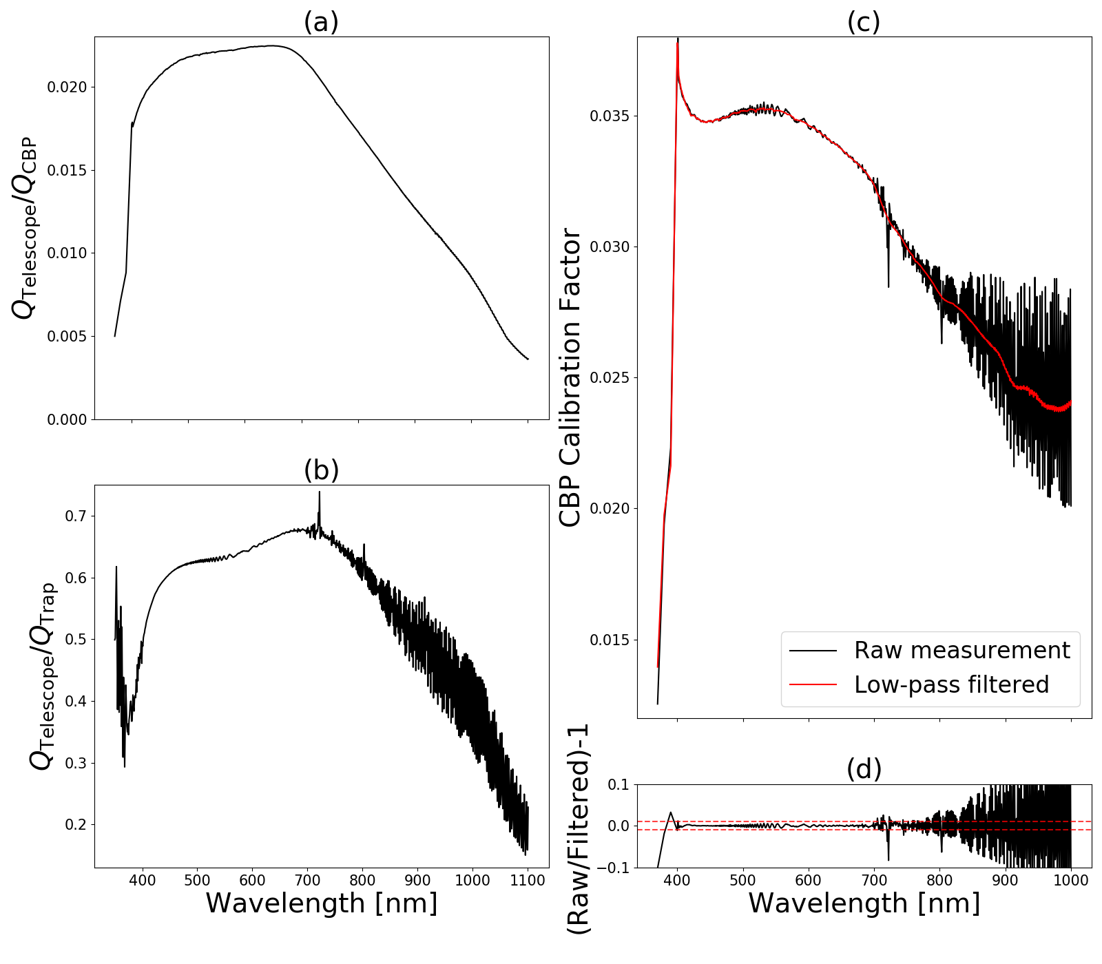
Figure 4: Results from the calibration chain described in Sec. 4. (a): Ratio between calibrated photodiode response and CBP monitor photodiode response. (b): Ratio between calibrated photodiode response and trap detector response. (c): The calibration factor of the CBP. The red curve has been low-pass filtered to suppress the interference fringe signal from the calibration telescope-trap measurement. (d): The relative difference between the raw and low-pass filtered CBP system throughputs, with dashed red lines drawn at $+/-1$ %. The sharp cutoff at approximately 400 nm seen in (a) and (c) is attributed to the AR coating on the CBP lens. The residuals in (d) are used to estimate the systematic CBP calibration uncertainty due to fringing.

5 CBP measurements of the StarDICE telescope transmission

5.1 The StarDICE experiment

The StarDICE experiment aims at anchoring fluxes of currently used spectrophotometric standard stars (SPSS) to the scale defined by POWR. In order to reconstruct fluxes that are free of atmospheric effects, the experiment envisions a long duration follow-up of SPSS ground level fluxes with a dedicated telescope, whose absolute full pupil transmission is monitored for the duration by observations of a calibrated artificial star with NIST traceability. The strategy is to average out the atmospheric transmission variations, given a long enough lever arm in time, and to use slitless spectro-photometry to constrain the absorption spectrum of the atmosphere. The details of this procedure will be left to a set of forthcoming papers (StarDICE collaboration, 2023-2024), but are expected to build up on the successed achieved by cosmological supernovae surveys, as for exampled described in [7].

A simple approach for the artificial star is to achieve quasi-perfect plane-wave illumination of the telescope by the observation of spherical waves emitted by small light sources in the long (but finite) distance range. In practice, the exercise is easier to achieve for small apertures, for which the long range remains within 200 m.

A test of the proposed concept was performed in 2018 at the Observatoire de Haute Provence (OHP) with a 10” f/4 Newtonian telescope. The focal plane of the telescope was equipped with a SBIG ST-7XME camera behind a 5 slot filter wheel with $bvRI$ filters and 1 empty slot. The $b$ and $v$ filters were interference filters, while the $R$ and $I$ filters were colored glass. The camera sensor is a grade 1 front-illuminated Kodak kaf-0402ME CCD, cooled to $\sim-10~{}^{\circ}$C using a Peltier junction for cooling. The $6.91$ mm$\times 4.6$ mm active area is divided into $765\times 510$ regions of $9~{}\mu$m$\times 9~{}\mu$m pixels.

A set of 18 narrow-spectrum LEDs, attached 113.4 m away from the primary mirror vertex, were observed at the beginning and end of each observation night to monitor the evolution of the instrument throughput around 18 different wavelengths, the rest of the night being devoted to the photometric follow-up of SPSS in 4 $bvRI$ filters. The test demonstrated a sub-percent precision of the nightly calibration by the point-like artificial star, while collecting photometry for a handful of SPSS with $\sim 0.01$ mag photon statistics on individual images. The test was put to a halt by a sudden and rapid change in the apparent instrument throughput. The subsequent analysis of calibration data demonstrated that the evolution was entirely attributable to a change of the sensor readout electronic gain, with no apparent change of the detector quantum efficiency according to the artificial star observations.

We present here a measurement of the monochromatic throughput of this test instrument that is necessary to interpret the broadband stellar and LEDs measurements. The measurement is occuring a posteriori, using the impaired sensor. The sensor readout gain appears to have settled at a different but stable value, so that the most adverse effect is an increased readout noise, to around 16 e^-. We stress for clarity that none of the measurements done at OHP are discussed here. We only report the procedure done a posteriori at the lab to characterize the telescope and filters used in the StarDICE demonstration program.

5.2 Experimental setup

The CBP system was set up in the StarDICE lab at LPNHE, with the CBP collimator approximately 1.5 m away from the StarDICE primary (see Fig. 1). Images were taken in dark/light pairs – for “dark” images, the StarDICE camera shutter was opened, but the laser shutter remained closed. Subtraction of these image pairs then corrects for scattered light from contaminating sources. For charge measurement, the CBP electrometer was configured to take 10 readings before and after closing the laser shutter, which permits measurement of background photodiode charge levels. During exposures, the monitor spectrograph was continually read out and saved at a fixed rate, typically 1 Hz or 10 Hz, depending on total exposure time. The telescope CCD’s exposure time includes an additional $t_{\mathrm{buffer}}=10$ seconds relative to the requested exposure time from the CBP ($t_{exp}$), in order to allow for communication between the telescope and CBP systems. Upon completing the exposure, the photodiode and spectrograph time-series are stored alongside the image. The CBP scan procedure can be summarized as

1. Open StarDICE camera shutter, laser shutter remains closed. Expose for time $t_{\mathrm{exp}}+t_{\mathrm{buffer}}$. Close camera shutter. Used as background subtraction image for following exposure.

2. Open StarDICE camera shutter. Reset electrometer charge and take 10 charge measurements. Begin taking spectrometer measurements.

3. Open laser shutter, expose for time $t_{\mathrm{exp}}$. The exposure time is chosen in order to yield enough signal in the camera detector without saturating the photodiode. As will be discussed later on, this didn’t ensure the spectrograph signal to be unsaturated. This issue has been taken care of in the new setup.

4. Close laser shutter, take final 10 readings on electrometer, stop spectrometer integration.

5. Close StarDICE shutter, move to next wavelength, repeat.

In this setup the grid of pinholes is used, in order to test the multiplexing of the transmission measurement at many different locations on the camera detector.

6 Data reduction

6.1 Photometry

To measure the amount of photons collected by the CCD, we perform aperture photometry on the grid of points imaged onto the focal plane. The magnification ratio between the telescope and the CBP collimating optic is roughly 4; this means the 20 $\mu$m holes in the CBP mask become 80 $\mu$m diameter spots on the StarDICE focal plane, which translates to about 9 pixels. Because there are refractive optical elements in the telescope beam (e.g., filters, dewar window), the focus of the system will change slightly with wavelength though the amount of defocus is not large relative to the size of the spots. Beyond simple defocus, during the telescope’s trip back to LPNHE from its first calibration run at OHP (Observatoire de Haute Provence) , we believe that the telescope was knocked slightly out of collimation, leading to moderate aberrations in the images generated by the CBP. These aberrations are not prohibitively large, and can be accommodated by slightly increasing the aperture size used for photometric measurements. Fig. 5 shows an example of a bias corrected, dark frame subtracted image, with the individual aperture and background subtraction regions marked. In the analyses that follow, only spots whose entire photometry and sky background apertures lie entirely within the frame are used. We use an aperture of 45 pixels, with a background annulus of inner radius 50 pixels, and a width of 10 pixels. When measuring regions of very low transmission, forced aperture photometry is performed at the last known location of the pinholes.

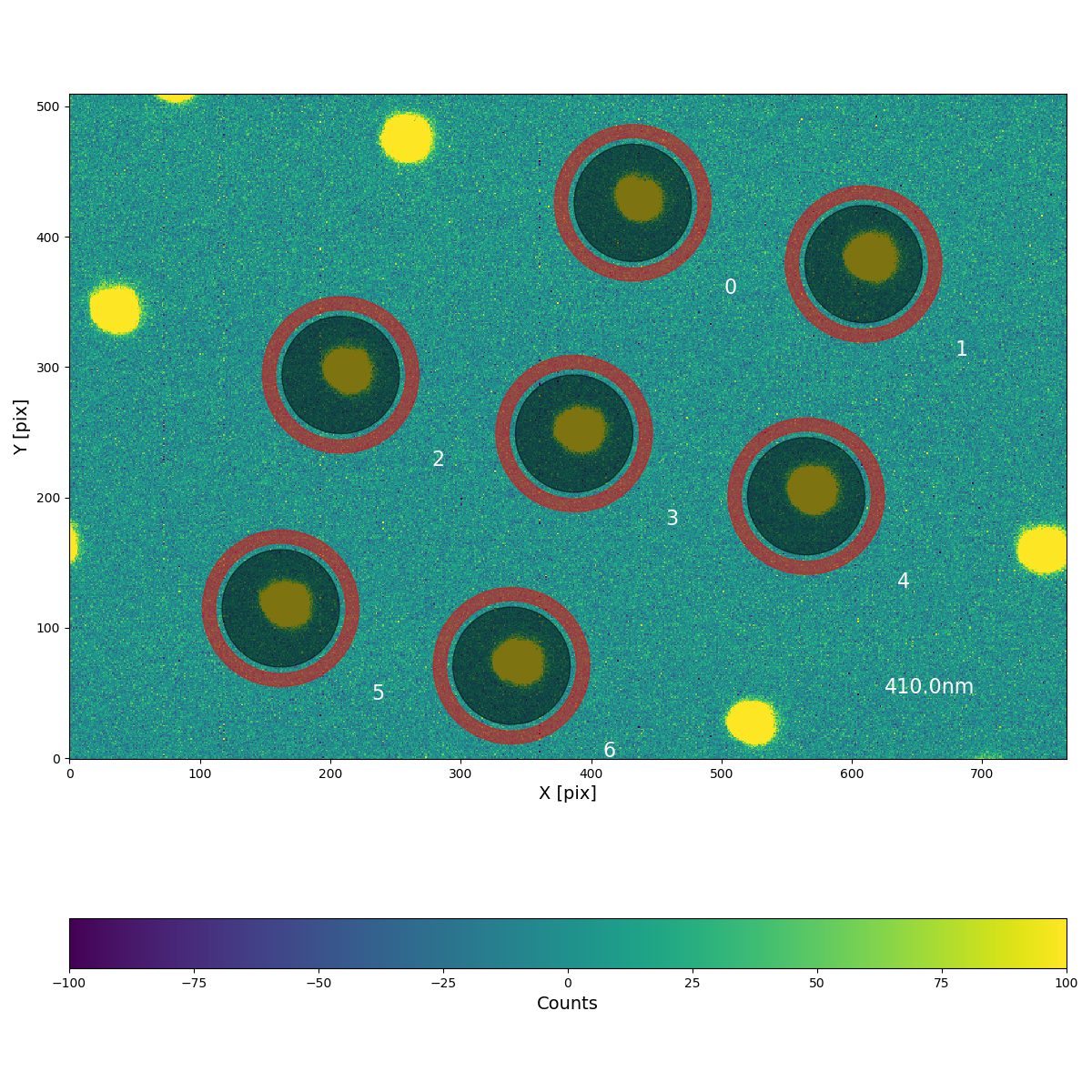
Figure 5: An image of the 5x5 20 $\mu$m pinhole mask as seen by the StarDICE CCD. The image has been bias corrected and differenced with a dark frame. Note that a very aggressive stretch is applied in order to see the wings of the spots, and that their size in terms of their full-width at half-max (FWHM) is much smaller. The black shaded regions indicate the apertures used for photometry, while the red annuli indicate regions used for background subtraction. White numbers label each spot, and the wavelength of the laser is shown in the lower right.

On occasion, we have noticed changes of a few pixels in the positions of the pinhole grid across the focal plane. These arise in particular when changing filters, though on occasion they seem to arise from presumed slippage in the alt/az motors driving the CBP pointing. We compensate for this by allowing the apertures to move as a fixed grid, with the new locations being determined via peak finding after convolving the image with a 2-d gaussian with a standard deviation of 10 pixels in x and y. Only in the case where all pinholes move uniformly is the pixel grid allowed to move. This prevents wandering apertures in cases where the transmission is effectively zero.

6.2 Charge measurement

Photocurrent generated in the monitor photodiode is integrated by the electrometer, and afterwards is used to normalize away variations in the input laser light intensity. We integrate charge rather than measure current in order to better account for the laser’s pulse-to-pulse instability, which can be of order 10 % or more. Measurements are made with the electrometer range fixed to 2 $\mu$C to avoid spurious jumps in charge levels that arise when the measurement range is changed. Typical charge levels reached by the CBP during an integration are (0.1 to 2) $\times 10^{-7}$ C. Bias current for the Keithley 6514 is specified to be $<4$ fA, which is negligible given our signal levels and integration times ($\leq 300$ s). Although the specification published in the 6514 datasheet provides only measurement accuracy (not precision), the manufacturer indicates that the value is intended to be understood as total measurement uncertainty, including both precision and accuracy. We therefore use the datasheet’s uncertainty formula for the 2 $\mu$C range given by

$$\sigma_{\mathrm{PD}}=0.01Q_{\mathrm{PD}}+500~{}\mathrm{pC}$$ (6)

as the uncertainty on the photodiode charge measurement. We keep the bias part of the formula in order to account for its variation throughout the experiment time span. We decided at this level to be conservative and defer the estimate of the non linearities and stability of the response to the next paper.

6.3 Spectroscopic Data and Calibration

The laser’s output wavelength is monitored by an Ocean Optics QE65000 spectrograph. The spectrograph is attached to the CBP integrating sphere by a 600 $\mu$m core diameter optical fiber, which also serves to define the entrance slit to the spectrograph. We read the device out at a rate of either 10 Hz or 1 Hz, depending on the brightness of the laser at the specified wavelength. The original choice of the fiber diameter was made in order to maximize the signal to noise ratio of the spectrograph readings over the full wavelength range.

To calibrate the spectrograph, an Ocean Optics HG-1 wavelength calibration lamp was shone into the CBP’s integrating sphere via an optical fiber, using the same integrating sphere entrance port as the laser input fiber.

The spectrograph calibration data has been analysed at the end of our data taking, after returning the laser to NIST. It was then noticed that the 600 $\mu$m diameter fiber was too broad to properly resolve the lines generated by the calibration source. Furthermore, we found that there was a systematic, wavelength-dependent shift in the PSF location between the small and large fiber, preventing a posteriori recalibration.

Since it was impossible to redo a full telescope scan with a smaller spectrograph fiber at that time, we were forced to rely on the stability of the wavelength provided by the laser given a fixed requested wavelength. Futher tests on a later CBP implementation with a similar but more recent laser showed that the relationship between the requested wavelength and the wavelength provided by the laser is extremely stable. Yet, for this paper we have no quantitative assessment of a potential shift of the wavelength calibration.

In summary, the wavelength calibration we use for the current analysis is as follows:

1. Spectrograph calibration using spectral lamps

2. Calibration of the relation between requested wavelength and the wavelength provided by the laser, using the spectrograph with the 100 $\mu$m fiber.

3. Use of this relation to transform requested wavelength into actual wavelength throughout our analysis of CBP data.

6.3.1 Spectrograph Calibration Procedure

We calibrate the spectrograph by directly linking it to an Ocean Optics Hg-1 lamp with a 100 $\mu$m diameter fiber.

We fit the calibration lamp spectra in pixel space using a model that is the sum of 20 gaussians (one per emission line) and a 0^th order polynomial for background estimation, and the results of the fit are shown in Fig. 6. We also note that there is a distinct lack of calibrated emission lines in the HG-1 lamp for $\lambda\gtrsim 950$ nm, thus the wavelength solution should not be trusted much beyond these values. Because our CBP calibration data set does not presently extend beyond 1000 nm, we mask the data for which $\lambda>1000$ nm (estimated a priori from the spectrograph’s built-in wavelength solution). To determine a wavelength-pixel mapping for the spectrograph, we fit the centers of the gaussians against the known calibration lines using a 3^rd order Chebyshev polynomials. The per-line residuals of this fit are shown in the lower panel, and the standard deviation of the lines about 0 indicates that the wavelength solution is good to approximately 0.3 nm.

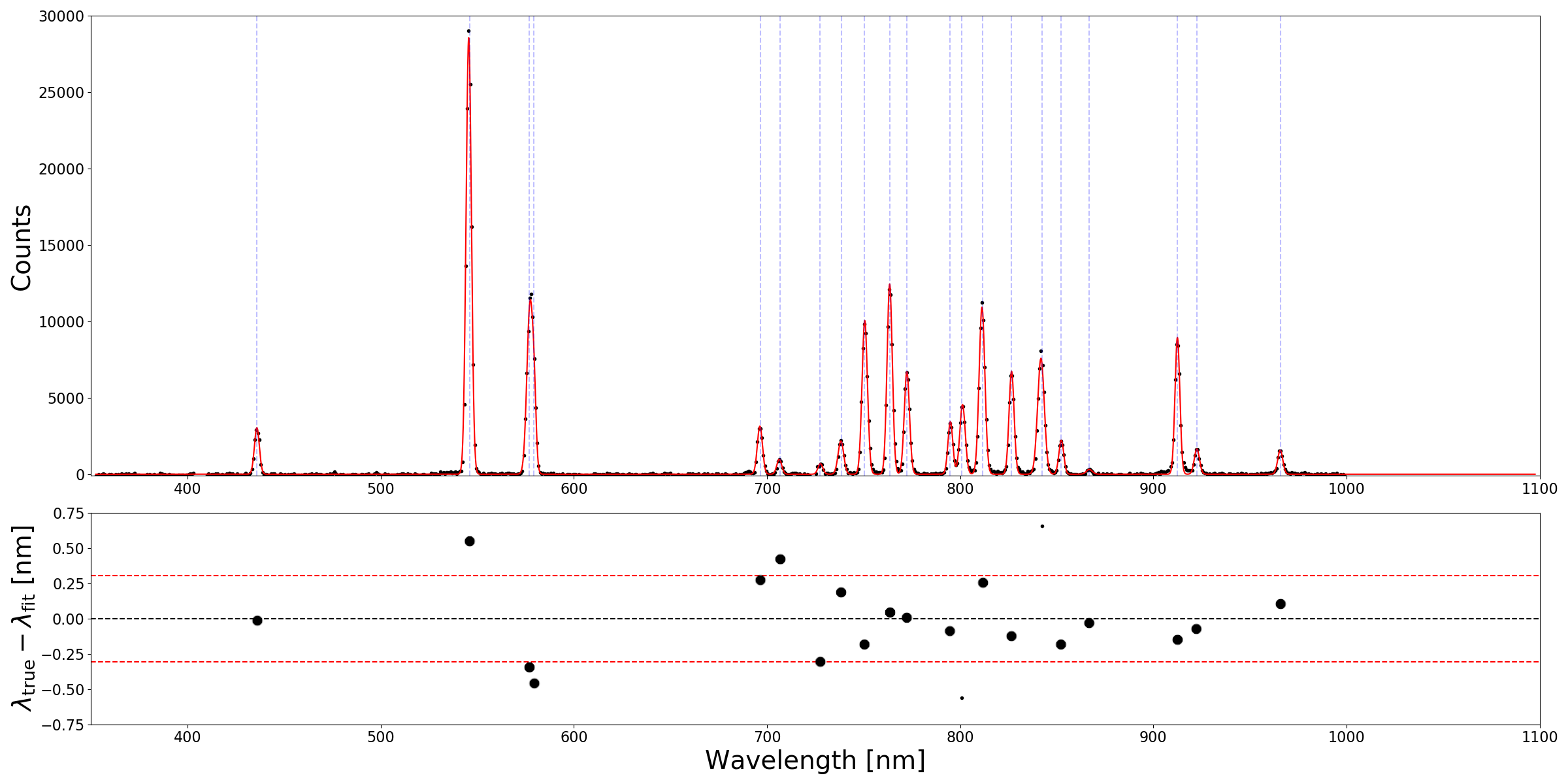
Figure 6: Calibration of the CBP monitor spectrograph with an Ocean Optics HG-1 calibration lamp. On the upper figure, data (black points) is plotted as a function of fitted wavelength and the red curve shows the fitted model. Pale blue dashed lines denote the true wavelengths of the calibration lines used in the fit. Data for $\lambda>1000$ nm are masked. The lower figure shows the difference between true and best-fit wavelengths for the calibration lines. Red dashed lines are drawn at $+/-1\sigma$ (= 0.32 nm) from the mean (dashed black line).

6.3.2 Calibration of the requested wavelength to calibrated wavelength relationship for the laser

We transfer this wavelength calibration to the laser by taking a series of laser output spectra, changing the laser wavelength by 20 nm between each spectra. We fit a gaussian to the laser line and then use a 3rd order Chebyshev polynomial to generate a mapping between requested laser wavelength and spectrograph measured wavelength. The results of this fitting process are shown in Fig. 7.

After applying the polynomial relationship between requested and measured wavelength, the residuals improve to approximately the 0.1 nm level. For the rest of the data presented here we use this polynomial calibration to infer the true output wavelength of the laser for a given requested wavelength.

We are aware of, and note the fact that the wavelength calibration uncertainty quoted here is but an estimate, that suffers from the limited amount of time and data available to write this report. A more detailed propagation of the wavelength calibration errors will be included in the next version of the experiment, that will be reported in the next forthcoming paper (Souverin et al. in prep.).

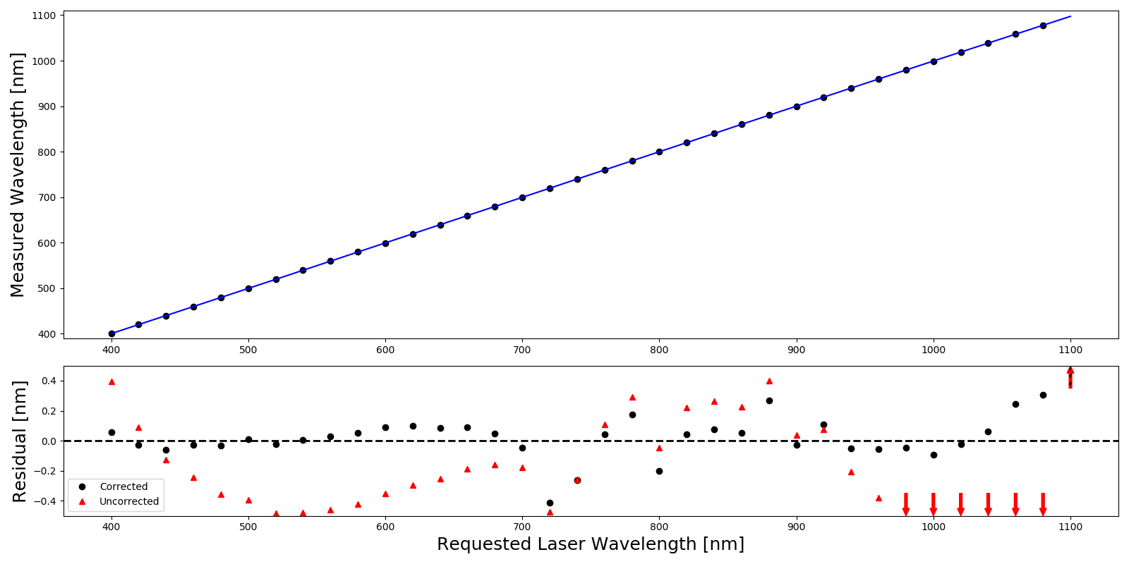
Figure 7: Upper panel: raw data (black dots) and fitted Chebyshev polynomial (blue line) showing the spectrograph measured wavelength as a function of wavelength requested from the laser. Lower panel: residuals from the fit (black points) as well as the original difference between resquested and measured wavelength (red triangles). The fit shows residuals at around the 0.1 nm level for most of the wavelength range of interest. Residuals that lie outside the bounds of the lower plot are denoted with arrows. The black and red hatched arrow indicates that the residual at 1100 nm lies outside the plot for both the corrected and uncorrected case.

6.4 Throughput Calculation

Mathematically, $T_{i}(t,\lambda,\textbf{x})=Q_{\mathrm{CCD,i}}(t,\lambda,\textbf{x})/(Q_{\mathrm{PD}}(\lambda)T_{\mathrm{CBP}}(\lambda))$, where $T_{i}$ is the (unnormalized) telescope transmission as seen by pinhole $i$, $Q_{\mathrm{CCD},i}$ is the charge collected by the CCD for pinhole $i$, $Q_{\mathrm{PD}}(\lambda)$ is the charge collected by the CBP monitor photodiode, and $T_{\mathrm{CBP}}(\lambda)$ is the transmission correction for the CBP system as outlined in Section 4. Because the true quantum efficiency of the CBP monitor photodiode is rolled into our CBP calibration term, there is no correction factor for the CBP monitor photodiode. The different pinholes allow for a degree of focal plane multiplexing by sampling different sections of the system within a single exposure. This provides potentially the ability to measure grey and chromatic variations of the full detector response.

To show the derivation for this form of $T_{i}$, we can first use Eqn. 3 to write

$$Q_{\mathrm{CCD},i}=\sum_{\mathrm{pix},i}\phi_{\mathrm{CBP}}(t,\textbf{x},\lambda)\Delta\,t$$ (7)

where the sum is over the pixels belonging to the image of pinhole $i$, which serves to localize the measurement to the region around point x on the focal plane, and $\Delta t$ is the integration time. We then arrive at the expression

$$Q_{\mathrm{CCD},i}(t,\lambda,\textbf{x})=\sum_{\mathrm{pixels},i}C(t)T(t,\lambda,\textbf{x})S_{\mathrm{pixel}}(t,\lambda,\textbf{x})\Delta\,t$$ (8)

where $S_{\mathrm{pixel}}$ is the photon flux seen by a given pixel in aperture $i$ such that $\sum_{\mathrm{pixels}}S_{\mathrm{pixel}}(t,\lambda,\textbf{x})=S(t,\lambda,)$, and we have invoked the approximation that the CBP is sampling a representative weighting of the StarDICE primary (allowing us to drop the r dependence), enabled by the coincidence that the CBP output beam size is roughly the size of the StarDICE primary annulus (We define the primary annulus as the primary disc hollowed out of the shade of the secondary). The calibration factor of the CBP monitor photodiode $T_{\mathrm{CBP}}$ has been transformed up to an arbitrary grey term, that we set to one for simplicity, asserting that each photoelectron corresponds to a single unique detected photon. The total number of photons entering the StarDICE telescope for a given pinhole, written as $S(\lambda,t)\Delta\,t\,K_{\mathrm{i}}$, is also given by $Q_{\mathrm{PD}}T_{\mathrm{CBP}}$, where $K_{i}$ is an unknown constant reflecting our ignorance of the true size of the emitting pinhole. By assuming that the transmission of the telescope system is reasonably flat over the size of the pinhole image on the detector, we can write the ratio $Q_{\mathrm{CCD,i}}/(Q_{\mathrm{PD}}T_{\mathrm{CBP}})$ as

$$\frac{Q_{\mathrm{CCD,i}}}{Q_{\mathrm{PD}}T_{\mathrm{CBP}}}=\frac{C(t)T(t,\lambda,\textbf{x}_{\mathrm{center}})\sum_{\mathrm{pixels,i}}S_{\mathrm{pixel}}(t,\lambda)\Delta\,t}{K_{\mathrm{i}}S(t,\lambda)\Delta\,t}=\frac{C(t)}{K_{\mathrm{i}}}T(t,\lambda,\textbf{x}_{\mathrm{center}})$$ (9)

where the term $\frac{C(t)}{K_{\mathrm{i}}}$ is a constant with respect to wavelength.

Under the assumption that the temporal variability of $C(t)$ (which is mostly related to variables such as electronic gain and grey extinction due to e.g., dust on the primary) is slow compared to the time needed to measure the transmission, we can treat the ratio as a constant, $C$. This constant is the same for all measurements of a given pinhole $i$ at location x for a given scan, and we can normalize it away by dividing by the transmission at a fiducial wavelength or by the average transmission over all wavelengths. This gives us a measurement of system transmission at time $t$ and focal plane position x relative to another wavelength, thus reaching our goal of measuring the relative throughput of the system.

In summary, the process of measuring throughputs with a CBP consists of performing aperture photometry on each of the pinhole images, dividing by the photodiode charge measurement and CBP calibration factor at that wavelength, and then normalizing by, for example, the average of that quantity over all wavelengths. We then obtain a set of relative transmissions, one per pinhole $i$, covering the entire detector, allowing to trace both the average transmission for a given CBP partial illumination of the primary mirror, and potential chromatic transmission variations over the field of view.

6.5 Throughput uncertainty calculation

Using the standard method for uncertainty propagation, the uncertainty on the throughput measurement $T=Q_{\mathrm{CCD}}/(Q_{\mathrm{PD}}T_{\mathrm{CBP}})$ is given by

$$\sigma_{T}=\big{(}(\frac{\partial T}{\partial Q_{\mathrm{CCD}}}\sigma_{\mathrm{CCD}})^{2}+(\frac{\partial T}{\partial Q_{\mathrm{PD}}}\sigma_{\mathrm{PD}})^{2}+(\frac{\partial T}{\partial T_{\mathrm{CBP}}}\sigma_{\mathrm{CBP}})^{2}\big{)}^{\frac{1}{2}}$$ (10)

where $\partial T/\partial Q_{\mathrm{CCD}}=1/(Q_{\mathrm{PD}}T_{\mathrm{CBP}})$, $\partial T/\partial Q_{\mathrm{PD}}=-Q_{\mathrm{CCD}}/(Q_{\mathrm{PD}}^{2}T_{\mathrm{CBP}})$, and $\partial T/\partial T_{\mathrm{CBP}}=-Q_{\mathrm{CCD}}/(Q_{\mathrm{PD}}T_{\mathrm{CBP}}^{2})$. The uncertainty budget for the CBP’s measurement of the StarDICE telescope’s no-filter throughput is shown in Fig. 8. For wavelengths below approximately 800 nm, the uncertainty is dominated by uncertainty in the charge measurement. From the definitions given above (equations 6 and 10), it is easy to show that the minimum uncertainty contribution from the photodiode term is 1%, in the limit that $50\mathrm{nC}<<Q_{\mathrm{PD}}$. Once the prescribed limit is reached, the photodiode uncertainty is not a function of total charge, and therefore decouples from our ability to reduce it by exposing longer, or using a brighter source. It can be reduced only by making more measurements. At wavelengths longer than $\sim 790$ nm, the CBP’s flux calibration (Section 4) is the limiting factor. In particular, the uncertainty ascribed to the interference fringing in the calibration transfer telescope.

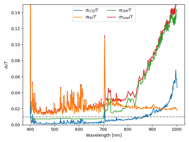
Figure 8: The uncertainty budget for the CBP measurement of StarDICE throughput. Contributions to the total uncertainty budget (red) are shown for the 3 main components: aperture photometry (blue), photodiode charge measurement (orange), and CBP calibration (green). The spike seen near 700 nm is due to the degeneracy region in the laser, and the spike near 400 nm is due to low laser brightness combined with low CBP optical throughput. The gradual rise from approx. 850 nm onward is believed to be due to the interference fringing effect discussed in Sec. 4.

7 Results and Discussion

7.1 StarDICE telescope transmission

Fig. 9 shows the transmission of the StarDICE telescope as measured by the average over all pinholes within a single CBP pointing. In order to examine the relative throughput of the system, we normalize each pinhole by its peak value with no filter in the beam, thereby allowing us to directly compare transmission variations across pinholes. The periodic variations seen in the transmission curves in the blue ($\lambda\lesssim 600$ nm) are believed to be real, and due to interference fringing in the microlens array mounted on the StarDICE CCD. Although not visible on the results plotted, we mention for completeness that there is also one point (810 nm, $I$ band) that is excised due to laser issues during the exposure.

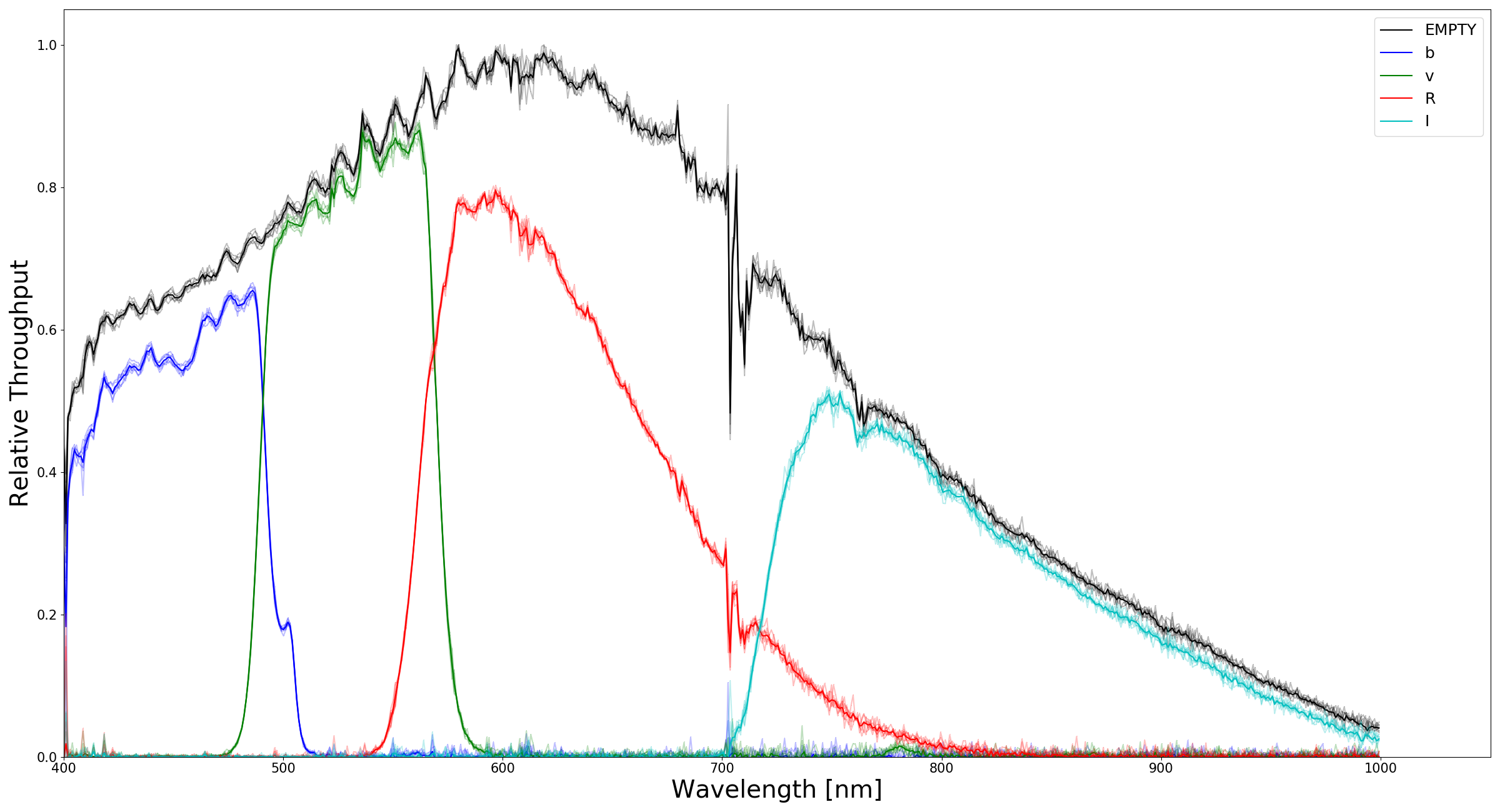
Figure 9: A multi-pinhole CBP scan of the StarDICE telescope. Each color represents a different filter placed in the beam of the telescope. The transparent curves show the measured transmissions for each of the pinholes in the grid, while the solid curves are the means across all pinholes. Each pinhole is normalized relative to its own peak value in the no-filter scan. The sharp features seen around 710 nm are due to extremely low SNR (signal-to-noise ratio), on account of the degeneracy region of the laser.

The data ends at 1 $\mu$m, as this is the cutoff wavelength for the trap detector calibration we currently have in hand. As the goal of this paper is to outline the performance of the CBP, we do not extrapolate the curve farther, nor implement an interpolation scheme for the degeneracy region and instead leave these elements of the StarDICE bandpass analysis to the forthcoming StarDICE experiment paper (StarDICE collaboration 2023-2024). In general the filters are well-behaved with one exception being a small leak in the $v$ filter around 790 nm. The sharp features around 710 nm are due to the degeneracy region of the laser, and are not true features of the StarDICE bandpass.

7.2 Evidence for variation across StarDICE focal plane

In addition to the average transmission measurement of Fig. 9, we report a chromatic variation of roughly 5 % for the CBP open transmission measurement (no filter) on a per-pinhole basis. This is shown on Fig. 10, where the crosses represent CBP measurements of the StarDICE telescope transmission over the full optical range, colored by pinhole number. They have been integrated over narrow ($\sim 30$ nm) bands for later comparison with LED flat field measurements of the camera transmission. We see that, relative to the measurement for pinhole 0, every other pinhole displays a chromatic evolution of the open transmission of about 5 % from 400 nm to 950 nm.

We also observe a systematic difference between pinholes, with pinholes 4-6 being more transmissive than others at 400 nm and less transmissive at 950 nm. This corresponds to a spatial evolution over the field of view of about 5 %.

Part of these effects can be accounted for by the camera response, as shown by the round coloured dots on the same figure. Those points represent the open transmission of the camera measured by flat field illumination using LEDs of narrow ($\sim 30$ nm) spectra. The flat fields obtained are integrated over spatial regions corresponding to each pinhole and displayed in the same color coding as the CBP measurements. We see that both the chromatic trend of all pinholes and the spatial trend between pinholes are partially accounted for by the response of the camera. A more quantitative assessment of the spatial variation detected would need a full range of new measurements, both with the CBP and with the flat field illumination system, which is beyond the scope of this paper. It nonetheless shows that a CBP is a promising tool to measure the response of the full telescope system down to the camera, even at the level of variations within the field of view.

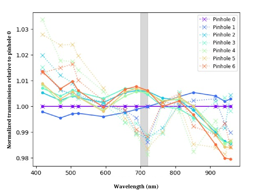
Figure 10: Normalized transmissions for each of the pinholes from the CBP scan of the StarDICE telescope. Xs denote CBP measurements integrated over the wavelength width of the LEDs used in the flat field study of the CCD. Circles signify LED flat field illumination measurements of the camera, integrated over 10 x 10 pixel squares at the position of the CBP pinholes. The grey strip denotes the degeneracy region, where CBP measurements are less reliable. Some evidence for spatial variability in the transmission function is seen, particularly in the blue end of the spectrum.

7.3 Reproducibility

In addition to the uncertainty calculations given in Section 6.5, we also obtained repeated measurements of the transmission function of the telescope at a fixed subset of wavelengths to test the robustness of the CBP results. Fig. 11 shows the results of 10 measurements of the StarDICE system throughput taken at 13 different wavelengths (50 nm intervals from 400 nm to 1000 nm) on a per-pinhole basis. Note that the pinholes and focal plane locations are not the same as those in Fig. 9. The measurements were taken as 10 sets of 13 measurements (i.e., the wavelength was changed between each measurement), which temporally separates the measurements at each wavelength by several minutes. Each pinhole-wavelength combination is normalized to its mean value, and horizontal colored lines are drawn at $+/-1\sigma$. Black horizontal lines denote the calibration uncertainty goal of 1 % (standard uncertainty), which is generally met between approximately 450 nm to 850 nm. This is in line with the theoretical predictions, which say that uncertainty should decrease by $1/\sqrt{N}$. For $N=10$ measurements, we would expect 1 % precision for measurements with individual uncertainties of $\sim 3~{}\%$ – this corresponds roughly to the 450 nm to 800 nm region in Fig. 8. This is because the uncertainty of the CBP photodiode charge measurements is statistics dominated in that spectral region. Where the systematic error due to the CBP transmission uncertainty dominates, the uncertainty doesn’t decrease with repeated measurements.

The grey shaded regions are visualizations of this uncertainty for each wavelength. The under-estimation of the predicted uncertainty and the observed scatter is likely due to the very sharp nature of the AR coating cutoff around 400  nm, and the calibration consequences thereof.

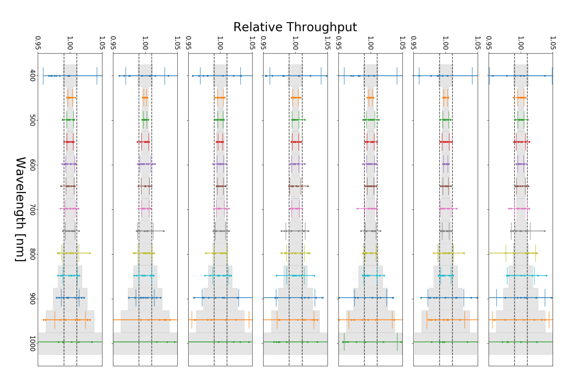
Figure 11: Repeatability test of the telescope transmission measurement from 400 nm - 1000 nm at 50 nm intervals. Each plot represents an individual pinhole on the StarDICE focal plane. The horizontal colored bars at each wavelength represent +/-1$\sigma$ from the mean of the measurements. Each data point is normalized by the mean of the measurements at that wavelength for that pinhole spot. For some of the measurements, the +/-1$\sigma$ lines fall slightly outside the limits of the graph. The dashed grey lines denote +/-1 % deviation from the mean. Solid grey regions denote predicted uncertainty using the total uncertainty budget from Fig. 8.

7.4 Additional Sources of Systematic Error

We have attempted, where practical, to maintain an accurate uncertainty budget for the CBP system. Here we discuss other possible sources of systematic uncertainty which might affect our measurements, and offer some possible future avenues of estimation or suppression.

One assumption we have made in the design of the CBP is the achromaticity of the pinhole grid illumination by the integrating sphere. If the back illumination of the grid is chromatic across the grid, that would directly translate to spurious chromatic evolution across the detector on the StarDICE system. Examining this would involve rotating or translating the detector under examination with respect to the CBP grid. By comparing data taken with the same spot at different areas of the focal plane (or different spots at the same area of the focal plane), we can place constraints on the achromaticity of the CBP pinhole illumination. Alternatively, if one wishes to quash this source of uncertainty at the expense of multiplexing, a single on-axis pinhole can be used, which will not suffer from this effect. We have plans to continue to explore this potential systematic on the StarDICE system in the future.

Another assumption is that the CBP calibration factor, which was measured at NIST with a single on-axis 500 $\mu$m pinhole (for SNR reasons), is directly transferable to the pinhole grid, with pinholes of significantly smaller sized and with most (if not all) of them at least slightly off axis. Measuring transfer achromaticity directly is challenging because the 500 $\mu$m pinhole has an area, and therefore signal, that is 25x larger than the total pinhole area of the 5x5 20 $\mu$m pinhole grid (and 625x larger than any individual pinhole). Repeating the NIST calibration process with this much less flux is a challenging proposition, and out of the scope of this paper. The assumption of calibration invariability with pinhole size will be a source of systematics investigated in details in the forthcoming paper (Souverin et al. in prep.).

Electronic gain variation represents another axis of systematic uncertainty. Gain drifts might occur in either the CCD readout electronics or in the electrometer; in either case, if the gain varies systematically over the course of a CBP scan, it would show up as a change in system response with wavelength. There is a method to counter this, which is to consistently return to a reference configuration (in both pointing and wavelength) during the scan. By taking data in the exact same configuration, any temporal drift in the electronics during the scan can be monitored and regressed away.

8 Conclusion

We have presented here the Collimated Beam Projector (CBP) which is a telescope transmission calibration device. The CBP uses collimated light to illuminate a telescope, mimicking a stellar wavefront over a subsection of the primary. By calibrating the output of the CBP relative to a NIST trap detector, the CBP can propagate the state-of-the-art POWR calibration to a telescope detector.

To demonstrate this, we have measured the throughput of the StarDICE telescope, with uncertainties between 3 % ($400$ nm $\lesssim\lambda\lesssim 800$ nm) and 14 % ($800$ nm $\lesssim\lambda\lesssim 1000$ nm). Over the full wavelength range, the wavelength calibration achieved, relying on the stability of the laser, is estimated to be of the order of 0.1 nm.

In its present form, precision for the CBP is limited by different factors in each of the regimes mentioned. In the short wavelength regime, the accuracy of the electrometer used to measure charge deposited on the monitor photodiode limits single-exposure uncertainties to 1 %, even at high flux. For the long wavelength region, we are limited by systematics in the calibration of the CBP, which arise due to interference fringing in the transfer telescope used in the calibration process.

To address the former limitation, two possibilities exist: make $N$ measurements and average, or procure a different, higher precision, electrometer. As an example, the Keithley 6517B electrometer has a per-measurement precision of 0.4 % + 50 pC for the 2 $\mu$C measurement range, which is a significant improvement over the 6514 used in this work. Making $N$ measurements to improve SNR is one of the improvements that have been implemented with success in futher work.

In the long wavelength regime, we are considering two avenues of approach: recalibration at NIST using a different optical setup using a reflective instead of refractive telescope to avoid fringing issues, or re-designing the collimation scheme for the CBP such that a monitor photodiode can be inserted directly to the output beam (rather than the integrating sphere). This latter scheme also has the advantage in that it requires only the calibration of the monitor photodiode relative to POWR, and not the calibration of the full CBP instrument, and is the path we have selected for our further developments. The main issue of having an output flux largely diluted at the output of the CBP, resulting on a signal too low to be accurately measured has been overcome by the use of a large surface solar cell that collects the entire output beam. The calibration of such a solar cell is described in [25] and its use will be discussed in a forthcoming paper (Souverin et al. in prep.).

In general, this implementation of a CBP in front of a telescope in a controled laboratory setting has provided many useful venues for improvement. Those have been implemented and will be presented in the forthcoming paper (Souverin et al. in prep.).

A calibration system that can be taken to different telescopes is of critical importance to supernova cosmology in particular, as photometric calibration has been and remains a major factor in determining cosmological parameters[2, 6, 26, 27]. In support of this mission, our group intends to undertake a series of measurements on a representative group of telescopes that have played significant roles in supernova measurements. In addition to our CBP, Rubin Observatory has also procured a CBP. Measurements and techniques learned here will be directly translated to support observations taken by the Rubin Observatory, and ultimately support the transfer of the NIST optical flux scale to astrophysical objects.

Biographies and photographs of the other authors are not available.