Recall, Robustness, and Lexicographic Evaluation

Abstract.

Researchers use recall to evaluate rankings across a variety of retrieval, recommendation, and machine learning tasks. While there is a colloquial interpretation of recall in set-based evaluation, the research community is far from a principled understanding of recall metrics for rankings. The lack of principled understanding of or motivation for recall has resulted in criticism amongst the retrieval community that recall is useful as a measure at all. In this light, we reflect on the measurement of recall in rankings from a formal perspective. Our analysis is composed of three tenets: recall, robustness, and lexicographic evaluation. First, we formally define ‘recall-orientation’ as sensitivity to movement of the bottom-ranked relevant item. Second, we analyze our concept of recall orientation from the perspective of robustness with respect to possible searchers and content providers. Finally, we extend this conceptual and theoretical treatment of recall by developing a practical preference-based evaluation method based on lexicographic comparison. Through extensive empirical analysis across 17 TREC tracks, we establish that our new evaluation method, lexirecall, is correlated with existing recall metrics and exhibits substantially higher discriminative power and stability in the presence of missing labels. Our conceptual, theoretical, and empirical analysis substantially deepens our understanding of recall and motivates its adoption through connections to robustness and fairness.

1. Introduction

Researchers use the concept of ‘recall’ to evaluate rankings across a variety of retrieval, recommendation (Zhao et al., 2022), and machine learning tasks (Sajjadi et al., 2018; Rudinger et al., 2015; Flach and Kull, 2015). ‘Recall at $k$ documents’ ($\text{R}_{k}$) and R-Precision (RP) are popular metrics used for measuring recall in rankings. And, while there is a colloquial interpretation of recall as measuring coverage (as it might be rightfully interpreted in set retrieval), the research community is far from a principled understanding of recall metrics for rankings. Nevertheless, authors continue to informally refer to evaluation metrics as more or less ‘recall-oriented’ or ‘precision-oriented’ without a formal definition of what this means or quantifying how existing metrics relate to these constructs (Kazai and Lalmas, 2006; Montazeralghaem et al., 2020; Dai et al., 2017; Mohammad et al., 2018; Li et al., 2014; Diaz, 2015).

The lack of a principled understanding of or motivation for recall has caused some to question whether recall is useful as a construct at all. Cooper (1968) argues that recall-orientation is inappropriate because user search satisfaction depends on the number of items the user is looking for, which may be fewer than all of the relevant items. Zobel et al. (2009) refute several informal justifications for recall: persistence (the depth a user is willing to browse), cardinality (the number of relevant items found), coverage (the number of user intents covered), density (the rank-locality of relevant items), and totality (the retrieval of all relevant items). So, while many ranking experiments compute recall metrics, precisely what and why we are measuring remains vague.

In this light, we approach the measurement of recall in rankings from a formal perspective, with an objective of proposing a new interpretation of recall with precise conceptual and theoretical grounding. Our analysis is composed of three interrelated tenets: recall, robustness, and lexicographic evaluation. First, we formally define ‘recall-orientation’ as sensitivity to movement of the bottom-ranked relevant item. Although simple, this definition of recall connects to both early work in position-based evaluation as well as recent work in technology-assisted review. Moreover, by formally defining recall orientation, we can design a new metric, total search efficiency, that precisely measures recall. Second, we analyze our concept of recall orientation from the perspective of robustness with respect to possible searchers and content providers in a disaggregated, population-based metric. Inspired by recent work in fairness, we define a notion of worst-case retrieval performance across all possible users. We further demonstrate that recall—and total search efficiency specifically—measures worst-case robustness. Finally, we extend this conceptual and theoretical treatment of recall by developing a practical preference-based evaluation method based on lexicographic comparison. Through extensive empirical analysis across 17 TREC tracks, we establish that our new evaluation method, lexirecall, is correlated with existing recall metrics but exhibits substantially higher discriminative power and stability in the presence of missing labels. While conceptually and theoretically grounded in notions of robustness and fairness, lexirecall pragmatically is appropriate when we are concerned with understanding system behavior for users who are focused on finding all relevant items in the same way that experiments adopt reciprocal rank as a high-precision metric. Our conceptual, theoretical, and empirical analysis substantially deepens our understanding of recall as a construct and motivates its adoption through connections to robustness and fairness constructs.

2. Preliminaries

We begin by defining our core concepts and notation in order to provide a clear foundation for our analysis. While many of these concepts will be familiar to those with a background in the information retrieval, we adopt a specific mathematical framework that will be important when proving properties of recall, robustness, and lexicographic evaluation.

We consider information retrieval systems that are designed to satisfy searchers with a specific information need in mind. Although a searcher’s information need is never directly revealed to the retrieval system, the searcher expresses an observable request to information retrieval system. A request can be explicit (e.g., a query or question in the context of text-based search) or implicit (e.g., engagement or rating history in the context of recommendation).

A system attempts to satisfy an information need by ranking all of the items in a corpus $\mathcal{D}$. A corpus might consist of text documents (e.g., a web crawl) or cultural media (e.g., a music catalog). And so, if $n=|\mathcal{D}|$, a retrieval system is a function that, given a request, produces a permutation of the $n$ items in the collection. As such, the space of possible system outputs is the set of all permutations of $n$ items, also known as the symmetric group of degree $n$ or $S_{n}$.

The objective of ranked retrieval evaluation is to determine the quality of a ranking $\pi\in S_{n}$ for the searcher. In the remainder of this section, we will detail precisely how we do this.

2.1. Relevance

The relevance of an item refers to its value with respect to a searcher’s information need. We adopt the notion of topical relevance, the match between an item and the general topic of the request (Boyce, 1982; Cooper, 1971). Specifically, we use binary topical relevance, where an item is considered relevant if any portion of the item–often a text document–would be valuable with respect to the information need. This is a conservative notion of relevance used by NIST’s Text Retrieval Conference (TREC) (Ruthven, 2014). Let $\mathcal{R}\subset\mathcal{D}$ be the set of documents labeled relevant to the request where $m=|\mathcal{R}|$.

Given a ranking $\pi$, then we define $p$ as the $m\times 1$ vector where $p_{i}$ is the position of the $i$th ranked relevant item in $\pi$. We present an example of how to construct $p$ in Figure 1. We will use $\overline{p}$ to represent the $m\times 1$ vector where $\overline{p}_{i}\in\mathcal{D}$ is the identity of the $i$th ranked relevant item. There are a total of $n\choose m$ unique $p$ and each unique $p$ corresponds to a subset of $C=m!(n-m)!$ unique permutations in $S_{n}$.

Figure 1. Relevance Projection with Imputation. Given set of relevant item ids $\mathcal{R}=\{083,107,511,668,820,977\}$, relevance projection of an incomplete top-10 ranking $\pi$ and relevant set $\mathcal{R}$ to a $m\times 1$ vector of positions $p$. We also show the inverse projection vector $\overline{p}$ of items at specific recall levels.

2.2. Permutation Imputation

Many ranking systems only provide a ranking on the top $\tilde{n}\ll n$ items, which may not include all relevant items, leaving elements of $p$ undefined. In order to use many metrics, especially recall-oriented metrics, we need to impute the positions of the unranked relevant items. An optimistic imputation would place the unranked relevant items immediately after the last retrieved items (i.e. $\tilde{n}+1,\tilde{n}+2,\ldots$). Such a protocol would be susceptible to manipulation by returning few or no items. Alternatively, we consider pessimistic imputation, placing the unretrieved relevant items at the bottom of the total order over the corpus. For example, if a system returns only three of six relevant items in the top $\tilde{n}$ at positions 2, 3, and 8, then we would define $p$ as,

$$p =\underbrace{2,3,8}_{\text{top $\tilde{n}$}},\underbrace{n-2,n-1,n}_{\text{bottom $n-\tilde{n}$}}$$

Pessimistic imputation is a conservative placement of the unretrieved relevant items and is well-aligned with our interest in robust performance. Moreover, it is consistent with behavior of metrics like rank-biased precision, which implicitly applies an exposure of 0 for unretrieved relevant items (i.e., for large $n$, $\lim_{i\rightarrow n}\gamma^{i}\approx 0$); and average precision, which implicitly applies an exposure of 0 for unretrieved relevant items (i.e., for large $n$, $\lim_{i\rightarrow n}\frac{1}{i}\approx 0$). We show an example of projection with imputation in Figure 1.

2.3. Measuring Effectiveness

When evaluating an information retrieval system, we consider two sets of important stakeholders: searchers and providers. Searchers approach the system with information needs and requests and ultimately define what is relevant. Providers contribute items to the search system which serve to satisfy searchers. Each item in the corpus is attributable, explicitly or not, to a content provider. In this section, we will characterize a broad family of evaluation metrics for these two sets of users that will allow us, in subsequent sections, to define formal notions of recall and robustness.

2.3.1. Measuring Effectiveness for Searchers

For a fixed information need and ranking $\pi$, an evaluation metric is a function that scores rankings, $\mu:S_{n}\times\mathcal{D}^{+}\rightarrow\mathbb{R}^{*}$ where $\mathcal{D}^{+}$ is set of all subsets of $\mathcal{D}$ excluding the empty set. An evaluation metric, then, is a function whose domain is the joint space of all corpus permutations and possible relevance judgments and whose range is a non-negative scalar value. We are specifically interested in a class of metrics that can be expressed in terms of a summation over recall levels.

Definition 2.1.

Given a ranking $\pi\in S_{n}$ and relevant items $\mathcal{R}\in\mathcal{D}^{+}$, a recall-level metric is an evaluation metric defined as a summation over $m$ recall levels,

(1) $$\mu(\pi,\mathcal{R}) =\sum_{i=1}^{m}e(p_{i})z(i,m)$$

where $e:\mathbb{Z}^{+}\rightarrow\mathbb{R}^{*}$ is a strictly monotonically decreasing exposure function proportional to the probability that the searcher reaches rank position $i$ in their scan of the list; and $z:\mathbb{Z}^{+}\times\mathbb{Z}^{+}\rightarrow\mathbb{R}^{*}$ is a metric-specific normalization function of recall level and size of $\mathcal{R}$.

The product $e(p_{i})z(i,m)$ is a decomposition of what Carterette refers to as a ‘discount function’ into an explicit function that models exposure and another that addresses any recall normalization.

Within the set of recall-level metrics, we are further interested in the sub-class of metrics that satisfy the following criteria for ‘top-heaviness’.

Definition 2.2.

We refer to a recall-level metric as top-heavy if, for $j\in[0\mathrel{{.}\,{.}}\nobreak m)$,

$$\sum_{i=1}^{m}e(p_{i})z(i,m) \geq\sum_{i=j+1}^{m}e(p_{i})z(i-j,m-j)$$

Top-heaviness indicates that, in the event that there are unjudged, relevant items above the currently highest-ranked relevant items, the metric value must be greater than or equal to the metric value computed over the incomplete judgments. Because we deal with metrics that include functions of $m$, this is not an obvious property, but one that will be important as we consider incomplete judgments and relationships between possible users in Section 4.

Top-heavy recall-level metrics are a precise subclass of discounted metrics, covering a broad class of existing metrics such as average precision (AP), reciprocal rank ($\mathrm{RR}$), normalized discounted cumulative gain ($\mathrm{NDCG}$), and rank-biased precision ($\mathrm{RBP}$), where we define the exposure and normalization as,

$$e_{\text{AP}}(i) =\frac{1}{i} z_{\text{AP}}(i,m) =\frac{i}{m}$$

$$e_{\mathrm{RR}}(i) =\frac{1}{i} z_{\mathrm{RR}}(i,m) =\begin{cases}1&\text{if $i=1$}\\ 0&\text{otherwise}\end{cases}$$

$$e_{\mathrm{NDCG}}(i) =\frac{1}{\log_{2}(i+1)} z_{\mathrm{NDCG}}(i,m) =\left(\sum_{k=1}^{m}\frac{1}{\log_{2}(k+1)}\right)^{-1}$$

$$e_{\mathrm{RBP}}(i) =(1-\gamma)\gamma^{i-1} z_{\mathrm{RBP}}(i,m) =1$$

Beyond classic retrieval metrics, top-heavy recall-level metrics include non-traditional metrics such those based on linear discounting (e.g., $e_{\text{lin}}(i)=1-\frac{i}{n}$). This results in a much broader class of metrics than those normally considered, for example, in the formal analysis of retrieval metrics (Moffat, 2013; Amigó et al., 2013; Ferrante et al., 2015). As a result, while all top-heavy recall-level metrics satisfy some formal properties retrieval evaluation metrics, large subsets of top-heavy recall-level metrics may satisfy more. A detailed analysis of formal properties of top-heavy recall-level metrics can be found in Appendix A. As mentioned before, we can contrast this with Carterette’s decomposition which focuses on the decomposition of metrics into gain and discount components. In our case, we do not model gain, since we deal with binary relevance. Our exposure and normalization functions, then, precisely define a subset of Carterette’s discount functions that do not fit into his metric taxonomy since they do not consider recall normalization.

We focus on this class of metrics in order to prove properties of robustness in Section 4.

2.3.2. Measuring Effectiveness for Providers

For content providers, we define the utility they receive from a ranking $\pi$ as a function of their items’ cumulative positive exposure, defined as exposure of a provider’s relevant content. Let $\mathcal{R}^{\prime}\subseteq\mathcal{R}$ be the subset of relevant items belonging to a specific provider. Since $e$ captures the likelihood that a searcher inspects a specific rank position, we can compute the cumulative positive exposure as,

(2) $$\eta_{e}(\pi,\mathcal{R},\mathcal{R}^{\prime}) =\sum_{i=1}^{m}e(p_{i})\text{I}(\overline{p}_{i}\in\mathcal{R}^{\prime})$$

where $m$ and $p$ are based on $\mathcal{R}$. Unless necessary, we will drop the subscript $e$ from $\eta$ for clarity. We summarize our notation in Table 1.

Table 1. Notation

$\mathbb{Z}^{+}$	positive integers
$\mathbb{Z}^{*}$	non-negative integers
$\mathbb{R}^{+}$	positive reals
$\mathbb{R}^{*}$	non-negative reals
$S_{k}$	set of all permutations of $k$ items
$\mathcal{A}^{+}$	non-empty subsets of $\mathcal{A}$
$\mathcal{A}^{+}$	non-empty subsets of $\mathcal{A}$
$\text{I}:X\rightarrow\{0,1\}$	indicator function (i.e., returns 1 if $X$ is true; 0 otherwise)
$x_{-i}$	reverse index (i.e., $x_{k-i+1}$ for the $k$-dimensional vector $x$)
$\mathcal{D}$	corpus
$\mathcal{R}$	relevant set
$n$	size of corpus (i.e., $|\mathcal{D}|$)
$m$	size of relevant set (i.e., $|\mathcal{R}|$)
$\tilde{n}$	number of documents retrieved
$S_{n}$	set of all permutations of $\mathcal{D}$
$\tilde{S}_{n}$	subset of $S_{n}$ generated by multiple systems for a fixed request
$\pi$	permutation of $\mathcal{D}$
$p$	sorted positions of relevant items
$\overline{p}$	item ids of relevant items sorted by position
$C$	number of unique permutations in $S_{n}$ for a given $p$ (i.e., $m!(n-m)!$)
$\mu:S_{n}\times\mathcal{D}^{+}\rightarrow\mathbb{R}^{*}$	searcher evaluation metric
$\eta:S_{n}\times\mathcal{D}^{+}\rightarrow\mathbb{R}^{*}$	provider evaluation metric
$\mu(\pi,\mathcal{R})\mathrel{\stackrel{{\scriptstyle\makebox[0.0pt]{\mbox{\tiny rank}}}}{{=}}}\mu^{\prime}(\pi,\mathcal{R})$	$\mu$ and $\mu^{\prime}$ rank $S_{n}$ identically
$e:\mathbb{Z}^{+}\rightarrow\mathbb{R}^{*}$	exposure of position
$z:\mathbb{Z}^{+}\times\mathbb{Z}^{+}\rightarrow\mathbb{R}^{*}$	normalization function
$\mathcal{U}$	set of possible searcher information needs for a request
$\mathcal{V}$	set of possible providers for a request

2.4. Metric Desiderata

Because there is no consensus on a single approach to validate a new evaluation method, we adopt a collection of desiderata that capture both theoretical and empirical properties, including

• Theoretical justification. Are the formal foundations of the evaluation clearly grounded in a normative value? (Sections 4.1, 4.2)

• Theoretical novelty. Is the evaluation theoretically different from existing methods? (Section 4.3)

• Empirical correlation with existing metrics. Is the evaluation method empirically correlated with existing methods? (Section 6.2.1)

• Ability to distinguish between rankings. Is the evaluation method better able to distinguish between rankings compared to existing methods? (Section 6.2.2)

• Ability to distinguish between systems. Is the evaluation method better able to distinguish between systems compared to existing methods? (Section 6.2.3)

• Robust to missing labels. Is the evaluation method more robust to missing labels compared to existing methods? (Section 6.2.4)

Throughout this article, when we assess or compare evaluation methods, we will focus on these properties.

We note that, since the evaluation methods we develop in Sections 3 and 5 are based on non-utilitarian population-level aggregates of individually-focused utility metrics, validation with, for example, behavioral feedback (Carterette et al., 2012) or user studies (Sanderson et al., 2010) is not possible. In lieu of empirical validation, we emphasize both conceptual and theoretical properties of our evaluation methods, grounding them in the relevant work in philosophy and economics. This normative design of an evaluation method is consistent with recent work in the recommender system community (Ferraro et al., 2022; Vrijenhoek et al., 2021, 2022, 2023).

3. Recall

As mentioned in Section 1, the description of ranked retrieval metrics as ‘recall-oriented’ remains poorly defined, leaving the formal analysis of metrics for recall-orientation difficult. From a technical point of view, some work considers recall-orientation to be a binary criteria, dependent on whether a metric includes the recall base (i.e., $\mathcal{R}$) in order to be computed (Kazai and Lalmas, 2006; Sakai, 2006). This would include metrics that compute set-based recall at some rank cutoff (Tomlinson and Hedin, 2017; Cormack and Grossman, 2017) as well as metrics like AP and $\mathrm{NDCG}$. Using a set-based recall metric is particularly well-suited for recall-orientation in early stages of multi-stage ranking (Macdonald et al., 2013; Mohammad et al., 2018). A binary notion of recall-orientation does not capture that some metrics may be more recall-oriented than others. This captured, in part, by references to recall-orientation as related to the depth in the ranking considered by the searcher (Diaz, 2015). More frequently, authors appeal to metrics like AP and $\text{R}_{1000}$ as being recall-oriented without clear discussion of what this means (Montazeralghaem et al., 2020; Dai et al., 2017; Li et al., 2014; Hashemi et al., 2020). On the other hand, both Mackie et al. (2023) and (Magdy and Jones, 2010b) refer to $\text{R}_{1000}$ as recall-oriented but AP being precision-oriented. In light of the lack of consensus on recall-orientation, in Section 3.1, we propose a new quantitative view of recall-orientation based on the how sensitive a metric is for a searcher interested in finding every relevant item. This allows us to see recall-orientation along a spectrum and compare the degrees of recall-orientation of different metrics. In Section 3.2, based on this definition, we derive a new recall metric, total search efficiency.

3.1. Metric Orientation

We are interested in more precisely defining precision and recall as constructs to be measured in information retrieval evaluation. Although most evaluation metrics colloquially capture some aspects of both precision and recall, understanding the sensitivity to each remains vague. We can address this vagueness by approaching precision and recall as two extremes of recall requirements. At one extreme, precision as a construct reflects the satisfaction of a searcher who only needs exactly one relevant item, the minimum amount of retrievable content. We might find this in domains like web search. At the other extreme, recall as a construct reflects the satisfaction of a searcher who needs every relevant item, the maximum amount of retrievable content. Zobel et al. (2009) refers to this as the totality interpretation of recall, found in many technology-assisted review domains. Indeed, this perspective is supported by evaluation programs like the TREC Total Recall Track (Roegiest et al., 2015) and patent search (Lupu et al., 2017); and by metrics like ‘position of the last relevant ’ (Zou and Kanoulas, 2020).

We begin by defining the precision valence of a ranking of $n$ items as how efficiently a searcher can find the first relevant item. For a fixed request, assume that we have $m$ relevant items. The ideal precision valence occurs when the first relevant item is at rank position 1. The worst precision valence occurs when the first relevant item is at rank position $n-m+1$, just above the remaining $m-1$ relevant items. Similarly, we refer to the recall valence of a ranking as how efficiently a searcher can find all of the relevant items. The ideal recall valence occurs when the last relevant item is at position $m$ (i.e., below the other $m-1$ relevant items) and the worst precision valence when it is at position $n$.

In order to define the precision orientation of a metric, we measure the difference in the best case precision valence and worst-case precision valence for a given metric. Although there is only one arrangement of positions of relevant items where the top-ranked item is at position $n-m+1$, there are $n-1\choose m-1$ arrangements of positions of relevant items where the top-ranked item is at position 1. In order to control for the contribution of higher recall levels, we can consider, for the best case precision valence, the ranking with a relevant item at the first position and the remaining $m-1$ relevant items at the bottom of the ranking. Precision orientation, then, measures sensitivity for a searcher interested in one relevant item. We depict this graphically in Figure 2(a). Similarly, in order to define the recall orientation of a metric, we measure the difference in the best case recall valence and worst-case recall valence for a given metric. Although there is only one arrangement of positions of relevant items where the bottom-ranked item is at position $m$, there are $n-1\choose m-1$ arrangements of positions of relevant items where the bottom-ranked item is at position $n$. In order to control for the contribution of lower recall levels, we can consider, for the worst-case recall valence, the ranking with a relevant item at position $n$ and the remaining $m-1$ relevant items at the top of the ranking. Recall orientation, then, measures sensitivity for a searcher interested in all relevant items. We depict this graphically in Figure 2(b).

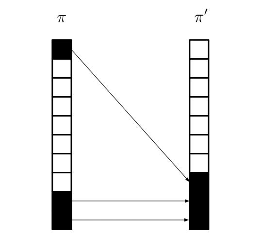
(a) Precision.

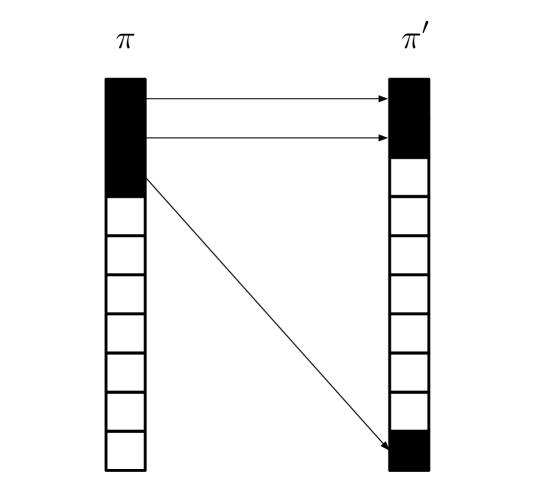
(b) Recall.

Figure 2. Metric orientation. Each ranking $\pi$ of ten items represented with a vector of cells ordered from top to bottom with shaded cells representing relevant items $\mathcal{R}$. Precision orientation (left) measures the degradation in a metric when the highest ranked relevant item is moved to the bottom of the ranking while holding all other positions fixed. Recall orientation (right) measures the degradation in a metric when the lowest ranked relevant item is moved to the bottom of the ranking while holding all other positions fixed. We measure the precision and recall orientation of a metric $\mu$ by the difference between $\mu(\pi,\mathcal{R})-\mu(\pi^{\prime},\mathcal{R})$.

In order to understand the intuition behind this definition of metric orientation, we can think about the recall requirements of precision-oriented or recall-oriented users. The prototypical precision-oriented user is satisfied by a single relevant item. Precision-orientation quantifies how sensitive a metric is at measuring the best-case and worst-case for this precision-oriented user. The prototypical recall-oriented user is only satisfied when they find all of the relevant items. Recall-orientation quantifies how sensitive a metric is at measuring the best-case and worst-case for this recall-oriented user. These prototypical users intentionally represent extremes in order to characterize existing metrics and control for any contribution from other recall requirements (e.g., those greater than one for precision and less than $m$ for recall).

Figure 3 shows the recall and precision orientation for several well-known evaluation metrics for a ranking of $n=10^{5}$ items. Because both precision and recall orientation are functions of the number of relevant items, we plot values for $m\in[1\mathrel{{.}\,{.}}\nobreak 15]$.

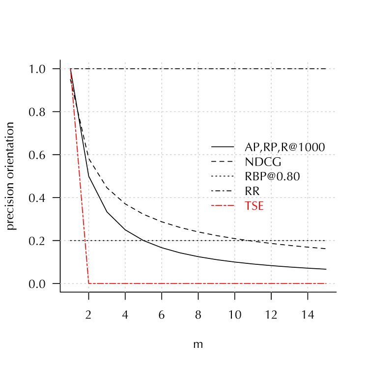
(a) Precision.

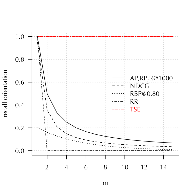
(b) Recall.

Figure 3. Metric orientation of ranking metrics of $10^{5}$ items with $m\in[1\mathrel{{.}\,{.}}\nobreak 15]$ relevant items. The vertical axis reflects, for $m\in[1,15]$, the change in metric value when (3(a)) moving top-ranked item from position 1 to position $n-m+1$ or (3(b)) moving bottom-ranked item from position $m$ to position $n$. The values for TSE (Equation 3) are scaled by the lower and upper bound given a fixed $m$ and therefore apply to any exposure model. See Figure 2 for details. This figure best rendered in color.

.

In terms of precision orientation, the ordering of metrics follows conventional wisdom. $\mathrm{RR}$ is often used for known-item or other high-precision tasks where the searcher is satisfied by the first relevant item. Across all values of $m$, $\mathrm{RR}$ dominates other metrics. $\mathrm{NDCG}$, often used for web search evaluation, is next more precision-oriented metric. AP, ‘recall at 1000’ ($\text{R}_{1000}$), and R-precision (RP) all have the same precision-orientation and are dominated by $\mathrm{NDCG}$. Rank-biased precision ($\mathrm{RBP}$) dominates $\mathrm{NDCG}$ and AP once we reach a modest number of relevant items. Both $\mathrm{RR}$ and $\mathrm{RBP}$ are not sensitive to the number of relevant items because neither is a function of $m$.

In terms of recall orientation, the ordering of metrics follows conventional wisdom in the information retrieval community. $\text{R}_{1000}$, AP, and RP all dominate other metrics for all values of $m$. This family of metrics is followed by metrics often used for precision tasks, $\mathrm{NDCG}$ and $\mathrm{RBP}$. $\mathrm{RR}$, the least recall-oriented metric, only considers the top-ranked relevant item and shows no recall orientation unless there is only one relevant item. We should note that, except for $\mathrm{RR}$, the recall orientation decreases with the number of relevant items because all of these metrics aggregate an increasing number of positions as $m$ increases. When evaluating over a set of requests with varying values of $m$, mis-calibrated recall valences may result in requests with lower values of $m$ dominating any averaging.

In this analysis, $\mathrm{RR}$ is a precision-oriented ‘basis’ metric insofar as it is only dependent on the position of the highest-ranked relevant item. We are interested in designing a symmetric recall-oriented ‘basis’ metric that only depends on the position of the lowest-ranked relevant item. We depict this desired metric as the red line in Figure 3. Traditional recall-oriented metrics do not satisfy this since they depend on the position of the higher-ranked relevant items, especially as $m$ grows. In this paper, we identify the missing metric that captures recall-orientation while being well-calibrated across values of $m$.

3.2. Total Search Efficiency

Although metrics such as AP are often referred to as ‘recall-oriented’, in this section, we focus on metrics that explicitly define recall as a construct.

Such recall metrics for ranked retrieval systems come in two flavors. The first flavor of recall metrics measures the fraction of relevant items found after a searcher terminates their scan of the ranked list. Metrics like $\text{R}_{1000}$ and RP use a model of search depth to simulate how deep a searcher will scan. We can define exposure and normalization functions for $\text{R}_{k}$ and RP,

$$e_{\text{R}_{k}}(i) =\text{I}(i\leq k) z_{\text{R}_{k}}(j,m) =\frac{1}{m}$$

$$e_{\text{RP}}(i) =\text{I}(i\leq m) z_{\text{RP}}(j,m) =\frac{1}{m}$$

Note that, although we decompose these metrics using the notation of recall-level metrics, neither of these exposure functions strictly monotonically decrease in rank, so they are not recall-level metrics.

The second flavor of recall metrics measures the effort to find all $m$ relevant items. Cooper (1968) refers to this as a the Type 3 search length and is measured by,

$$\text{SL}_{3}(\pi,\mathcal{R}) =p_{m}-m$$

$$\mathrel{\stackrel{{\scriptstyle\makebox[0.0pt]{\mbox{\tiny rank}}}}{{=}}}p_{m}$$

Similarly, Zou and Kanoulas (2020) uses ‘position of the last relevant document’ to evaluate high-recall tasks. By contrast, Rocchio (1964) proposed recall error, a metric based on the average rank of relevant items,

$$\text{RE}(\pi,\mathcal{R}) =\frac{1}{m}\sum_{i=1}^{m}p_{i}-\frac{m+1}{2}$$

$$\mathrel{\stackrel{{\scriptstyle\makebox[0.0pt]{\mbox{\tiny rank}}}}{{=}}}\sum_{i=1}^{m}p_{i}$$

Recall error can be sensitive to outliers at very low ranks, which occur frequently in even moderately-sized corpora (Magdy and Jones, 2010a).

Inspired by Cooper’s $\text{SL}_{3}$, we define a new recall-oriented top-heavy recall-level metric by looking at exposure of relevant items at highest recall level (i.e. $i=m$ in Equation 1). We can define a recall-oriented metric based on any top-heavy recall-level metric by replacing its normalization function with the following,

$$z_{\text{SL}_{3}}(i,m)=\begin{cases}1&\text{if $i=m$}\\ 0&\text{otherwise}\end{cases}$$

We refer to this as the efficiency of finding all relevant items or the total search efficiency, defined as,

(3) $$\operatorname{TSE}_{e}(\pi,\mathcal{R}) =\sum_{i=1}^{m}e(p_{i})z_{\text{SL}_{3}}(i,m)$$

$$=e(p_{m})$$

where the specific exposure function depends on base top-heavy recall-level metric (e.g., AP, $\mathrm{NDCG}$). TSE, then, is a family of metrics parameterized by a specific exposure function with properties defined in Section 2.3.1. Although computing $\operatorname{TSE}_{e}$ depends on the exposure model $e$, unless necessary, we will drop the subscript for clarity.

We demonstrate the precision and recall orientation of $\operatorname{TSE}$ in Figure 3. Since TSE with an AP base behaves identically to $\mathrm{RR}$, except from the perspective of recall-orientation, we consider it $\mathrm{RR}$’s recall-oriented counterpart. In the next section, we will connect this notion of recall to concepts of robustness and fairness.

4. Robustness

In the context of a single ranking, we are interested in measuring its robustness in terms of its effectiveness for different possible users who might have issued the same request. This is related to work in search engine auditing that empirically studies how effectiveness varies across different searchers issuing the same request (Mehrotra et al., 2017). In our work, we define robustness as the effectiveness of a ranking for the worst-off user who might have issued a request.

Underlying our notion of robustness is a population-based perspective on retrieval evaluation. Classic effectiveness measures can be interpreted as expected values over different user populations defined by different browsing behavior (Robertson, 2008; Sakai and Robertson, 2008; Carterette, 2011). For example, Robertson (2008) demonstrated that AP can be interpreted as the expected precision over a population of users with different recall requirements. More generally, Carterette (2011) demonstrated this for a large class of metrics. We can contrast this with online evaluation production environments where systems observe individual user behavior and do not need to resort to statistical models to capture different user behavior. So, just as recent work in the fairness literature disaggregates evaluation metrics to understand how performance varies across groups (Mehrotra et al., 2017; Ekstrand et al., 2018, 2022; Neophytou et al., 2022), we can disaggregate traditional evaluation metrics to understand how performance varies across implicit subpopulations of users such searchers or providers.

From an ethical perspective, when considered the expected value over a population of users, traditional metrics make assumptions aligned with average utilitarianism, where the expected utility over some population is used to make decisions (Sidgwick, 2011). While this reduces, in production environments, to averaging a performance metric across all logged requests, in offline evaluation, this is captured by the distribution underlying the metric, as suggested by Robertson (2008) and Carterette (2011). This means that if there are certain types of user behavior that are overrepresented in the data (online evaluation) or the user model (offline evaluation), they will dominate the expectation. Users whose behaviors or needs have low probability in the data or the user model will be overwhelmed and effectively be obscured from measurement.

For robustness, instead of measuring the effectiveness of a system by adopting average utilitarianism and computing the expected performance over users, we can summarize the distribution of performance over users using alternative traditions based on distributive justice. This follows recent literature in value-sensitive, normative design of evaluation metrics (Ferraro et al., 2022; Vrijenhoek et al., 2021, 2022, 2023). Specifically, inspired by related work in fair classification (Heidari et al., 2019; Hashimoto et al., 2018; Shah et al., 2021; Memarrast et al., 2021), we can adopt Rawls’ difference principle which evaluates a decision based on its value to the worst-off individual (Rawls, 2001). In the context of a single ranking, this means the worst-off searcher or provider. As such, our worst-case analysis is aligned with Rawlsian versions of 1 equality of information access (for searchers) and 2 fairness of the distribution of exposure (for providers) . Even from a utilitarian perspective, systematic under-performance can cost retrieval system providers as a result of user attrition (Hashimoto et al., 2018; Zhang et al., 2019; Mladenov et al., 2020) or negative impacts to a system’s brand (Srinivasan and Sarial-Abi, 2021).

Although motivated by similar societal goals (e.g., equity, justice), existing methods of measuring fairness in ranking are normatively very different from worst-case robustness. First, the majority of fair ranking measures emphasize equal exposure amongst providers (Ekstrand et al., 2022) and is based on strict egalitarianism, a different ethical foundation than Rawls’ difference principle (Rawls, 1974). Pragmatically, in order to satisfy this within a single ranking, authors restrict analysis to stochastic ranking algorithms (Singh and Joachims, 2018; Diaz et al., 2020) or amortized evaluation (Biega et al., 2018, 2019). Second, fair ranking analyses that focus on searchers tend be restricted to disaggregated evaluation, without reaggregating (Mehrotra et al., 2017; Ekstrand et al., 2018). This is different from our focus on disaggregating and then summarizing the distribution of effectiveness with the worst-off user. Most importantly, while most fairness work looks at either searchers or providers, in our analysis, we demonstrate that both worst-case searcher and provider robustness are simultaneously captured by recall, as measured by $\operatorname{TSE}$.

4.1. Searcher Robustness

Given a ranking $\pi$, we would like to measure the worst-case effectiveness over a population of possible searchers.

4.1.1. Possible Information Needs

Although topical relevance (Section 2.1) can be useful for evaluating generic information needs, a unique request can be submitted by a searcher as a result of any number of possible information needs. Harter (1992) uses the expression psychological relevance to refer to the extent to which, in the course of a search session, an item changes the searcher’s cognitive state with respect to their information need. Otherwise relevant items may stop being useful as a searcher’s anomalous state of knowledge changes (Belkin et al., 1982). Moreover, as Harter (1996) notes, because searchers approach a system from a variety of backgrounds (i.e., states of knowledge), two searchers issuing the same request might find quite different utility from items in the catalog. Empirically, we observe the variation in utility in controlled experiments (Voorhees, 1998; Voorhees and Harman, 1997) as well as production environments (Dou et al., 2007; Teevan et al., 2010). So, from this perspective, $\mathcal{R}$ should be considered the union of relevant items over all possible states of knowledge a searcher might have when approaching the system.

Indeed, multiple authors describe topical relevance as necessary but not sufficient for psychological relevance (Boyce, 1982; Ruthven, 2014; Cooper, 1971). These papers suggest that rather than seeing a retrieval system as acting to directly provide psychologically relevant items, it provides topically relevant items that are candidates to be scanned for psychologically relevant items by the searcher (Boyce, 1982).

There are numerous ways in which psychologically relevant items may manifest as a subset of topically relevant items. First, note that editorial relevance labels often are quite broadly defined, capturing notions of relevance that vary across different searchers or contexts. For example, the standard TREC relevance guidelines stipulate that, ‘a document is judged relevant if any piece of it is relevant (regardless of how small the piece is in relation to the rest of the document)’ (National Institute for Standards and Technology, 2000). Previous research has found that this liberal criteria, while surfacing most relevant documents, includes substantial marginally relevant content (Sormunen, 2002). As a result, some searchers may find a marginally relevant item irrelevant, effectively switching its label for that searcher. Or, a searcher may already be familiar with a judged relevant item in the ranking, which, in some cases, will, for that searcher, make the item irrelevant. For example, in the context of a literature review, a previously-read relevant article may not be useful to the search task; in the context of recommendation of entertainment content, the desirability of a previously-consumed relevant item may degrade due to satiation effects (Bookstein, 1979; Boyce, 1982; Leqi et al., 2021). Second, even if editorial relevance labels are accurate (i.e. all searchers would consider labeled items as relevant), the utility of items may be isolated to a subset of $\mathcal{R}$. For example, in the context of decision support, including legal discovery and systematic review, topical relevance is the first step in finding critical information (Cooper, 2016). In some cases, there will be a single useful ‘smoking gun’ document amongst the larger set of relevant content. In other cases, a single subset of relevant documents will allow one to ‘connect the dots.’ In a patent context, Trippe and Ruthven (2017) describe situations where there is risk to missing items that may turn out to be critical to assessing the validity of a patent.

So, while topical relevance is important, it only reflects the possible usefulness to the searcher (The Sedona Conference, 2009).

In light of this discussion, instead of considering any item in $\mathcal{R}$ as definitely satisfying the searcher’s information need, we consider it as only having a nonzero probability of satisfying the searcher’s information need.

Given that binary relevance reflects the possibility of psychological relevance, we are interested in considering all searchers such that the union of their relevance criteria is $\mathcal{R}$. We can enumerate all such searchers over items as $\mathcal{U}=\mathcal{R}^{+}$, the power set of $\mathcal{R}$ excluding the empty set. This means that, for a given request, we have $m^{+}=|\mathcal{U}|=2^{m}-1$ possible searchers interested in at least one relevant item (Figure 4). This conservative definition of $\mathcal{U}$ captures all possible satisfiable searchers.

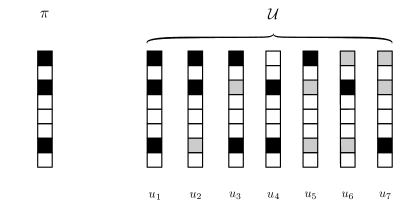
Figure 4. Population of possible searchers $\mathcal{U}$ based on all combinations of relevant items from $\mathcal{R}$ for a system ranking $\pi$.

4.1.2. Robustness Across Possible Information Needs

Given a set of possible information needs $\mathcal{U}$ based on $\mathcal{R}$, we define the robustness of a ranking $\pi$ as the effectiveness of the ranking for the worst-off searcher,

(4) $$\operatorname{WC}_{\mu}(\pi,\mathcal{R}) =\min_{u\in\mathcal{U}}\mu(\pi,u)$$

This is close to the notion of robustness proposed by Memarrast et al. (2021), who consider a worst-case searcher for whom relevant items have a marginal distribution of features that matches the distribution in the full training set. In comparison, our analysis considers the full set of worst-case situations, including those that do not match the training data.

One problem with this definition of robustness is that, because $m^{+}$ is exponential in $m$, computing the minimum is impractical even for modest $m$. Fortunately, using the properties of top-heavy recall-level metrics, we can prove that,

(5) $$\operatorname{WC}_{\mu}(\pi,\mathcal{R}) =\operatorname{TSE}(\pi,\mathcal{R})$$

In other words, the worst-off searcher is the one associated with $p_{m}$, the lowest-ranked relevant item. We present a proof in Appendix B.1. This result implies that recall orientation captures the utility of a ranking for the worst-off searcher.

4.2. Provider Robustness

Providers are individuals who contribute content to the information retrieval system’s catalog $\mathcal{D}$. Given a ranking $\pi$, we would like to measure the worst-case effectiveness over a population of possible providers.

4.2.1. Possible Provider Preferences

Just as with information needs, each ranking consists of exposure of multiple possible providers.

Consider the domains like job applicant ranking systems or dating platforms, where each item in the catalog is associated with an individual person. We assume that each relevant provider $i\in\mathcal{R}$ is interested in its cumulative positive exposure in the ranking (Section 2.3.2), $\eta(\pi,\mathcal{R},\{i\})$. In the more general case, providers can possibly be associated with multiple relevant items in $\mathcal{R}$. This might occur if a creator contributes multiple items to the catalog (e.g. multiple songs, videos, documents); or, a provider may aggregate content from multiple individual creators (e.g. publishers, labels). Even if we have metadata attributing groups of items to specific providers or creators, their preferences for exposure of those items may be unobserved. Provider preferences can themselves complex, covering a broad set of commercial, artistic, and societal values (Hadida, 2015; Eikhof and Haunschild, 2006).

Given the uncertainty and ambiguity over providers and their preferences, as with information needs, we can consider the full set of latent providers and their preferences, $\mathcal{V}=\mathcal{R}^{+}$ to reflect the set of possible provider preferences.

4.2.2. Robustness Across Possible Provider Preferences

Just as with searchers, we are interested in the utility of the worst-off provider. In the simple case where each provider is associated with a single item in $\mathcal{R}$, because exposure monotonically decreases with rank position, we know that the worst-off provider will be the one at the lowest rank; this is exactly $\operatorname{TSE}(\pi,\mathcal{R})$. This is similar to earlier provider fairness definition (Zhu et al., 2021). More generally, if, like information needs, we consider $\mathcal{V}=\mathcal{R}^{+}$, we define the worst-off provider as,

(6) $$\operatorname{WC}_{\eta}(\pi,\mathcal{R}) =\min_{v\in\mathcal{V}}\eta(\pi,\mathcal{R},v)$$

Given this definition, we can show that $\operatorname{TSE}$ is equal to the utility of the worst-case provider (proof in Appendix B.1).

Together, the results in Sections 4.1 and 4.2 provide a new interpretation of recall when viewed from the perspective of population-based evaluation. (Zobel et al., 2009)’s notion of totality shifts from being the desire of an individual searcher to being a measure of worst-off individual user.

Table 2. Agreement with $\operatorname{WC}_{\mu}(\pi,\mathcal{R})<\operatorname{WC}_{\mu}(\pi^{\prime},\mathcal{R})$. Probability of agreement over 10,000 simulated queries and pairs of random rankings for various corpus sizes. For each query, we selected $m\sim U(5,50)$ relevant items. We include the fraction of rankings tied under $\operatorname{WC}_{\mu}(\pi,\mathcal{R})=\operatorname{WC}_{\mu}(\pi^{\prime},\mathcal{R})$. The values for TSE apply to any exposure model.

$n$	tied	$\operatorname{TSE}$	$\text{R}@1000$	RP	AP	$\mathrm{NDCG}$	random
$10^{3}$	0.012	1.000	0.000	0.285	0.541	0.535	0.492
$10^{4}$	0.001	1.000	0.420	0.077	0.552	0.549	0.497
$10^{5}$	0.000	1.000	0.179	0.008	0.554	0.555	0.498
$10^{6}$	0.000	1.000	0.026	0.001	0.547	0.554	0.499

Figure 5. Dependence between $p_{1}$ and $p_{m}$. The gray region indicates the possible values of each.

4.3. Robustness and Existing Metrics

We have demonstrated that whenever $\operatorname{WC}_{\mu}(\pi,\mathcal{R})<\operatorname{WC}_{\mu}(\pi^{\prime},\mathcal{R})$, then $\operatorname{TSE}(\pi,\mathcal{R})<\operatorname{TSE}(\pi^{\prime},\mathcal{R})$. In order to understand the relationship between other metrics and worst-case performance, we simulate 10,000 requests by sampling 10,000 pairs of rankings $\pi$ and $\pi^{\prime}$. We can then compute the evaluation metric for each ranking and compare $\mu(\pi,\mathcal{R})<\mu(\pi^{\prime},\mathcal{R})$ with $\operatorname{WC}_{\mu}(\pi,\mathcal{R})<\operatorname{WC}_{\mu}(\pi^{\prime},\mathcal{R})$. We conduct this simulation for $n\in\{10^{3},10^{4},10^{5},10^{6}\}$ and present results in Table 2. We observe that, while $\operatorname{TSE}$ has perfect sign agreement with $\operatorname{WC}_{\mu}$, other recall-oriented metrics have worse agreement than random, largely because they only look at a prefix of $p$. The sign agreement of AP and $\mathrm{NDCG}$ is slightly better than random for two reasons. First, their aggregation (Equation 1) includes $p_{m}$ and will subtly affect the value, despite making a small contribution to the total sum. Second, $p_{i}$ values depend on each other because $\pi$ is a permutation. In Figure 5, we compare the possible joint values of $p_{1}$ and $p_{m}$. This means that we should expect there to be some dependence between purely precision-oriented metrics (e.g. $\mathrm{RR}$) and purely recall-oriented metrics (e.g. $\operatorname{TSE}$). That said, AP and $\mathrm{NDCG}$ agree less than $\operatorname{TSE}$ because their aggregation includes the positions of relevant items above $p_{m}$. In whole, this result suggests that, even compared to traditional recall metrics, $\operatorname{TSE}$ is better able to measure the robustness of a ranking.

5. Lexicographic Evaluation

In Section 3, we defined recall-orientation from the perspective of searchers interested finding in the totality of relevant items and then proposed a new metric, $\operatorname{TSE}$, based on this interpretation. In Section 4, we demonstrated how $\operatorname{TSE}$ measures the worst-case utility for multiple definitions of searchers and providers, connecting it to notions of robustness and fairness, through Rawls’ difference principle. In this section, we will further develop the fairness perspective by combining recent work in preference-based evaluation with classic work in social choice theory, improving the nuance in worst-case analysis and allowing it to be useful as an evaluation tool. We will begin by discussing the practical limitations of $\operatorname{TSE}$ for evaluation (Section 5.1) before developing a preference-based evaluation method derived from social choice theory that generalizes $\operatorname{TSE}$ and improves its practical use (5.2).

5.1. Low Sensitivity of Total Search Efficiency

Although measuring worst-case performance and, as a result, Rawlsian fairness, $\operatorname{TSE}$ may not satisfy our desiderata for an evaluation method (Section 2.4). To understand why, consider two rankings $\pi$ and $\pi^{\prime}$ for the same request. When comparing a pair of systems, we are interested if defining a preference relation $\pi\succ\pi^{\prime}$. The worst-case preference $\pi\succ_{\text{WC}}\pi^{\prime}$, is defined as,

(7) $$\pi\succ_{\text{WC}}\pi^{\prime} \leftrightarrow\min_{u\in\mathcal{U}}\mu(\pi,u)>\min_{u\in\mathcal{U}}\mu(\pi^{\prime},u)$$

We know from Section 4.1.2 that this can be efficiently computed as $\operatorname{TSE}(\pi)>\operatorname{TSE}(\pi^{\prime})$. Unfortunately, in situations where the worst-off user is tied (i.e. $\min_{u\in\mathcal{U}}\mu(\pi,u)=\min_{u\in\mathcal{U}}\mu(\pi^{\prime},u)$), we cannot derive a preference between $\pi$ and $\pi^{\prime}$. Because we assume that unretrieved items occur at the bottom of the ranking and because most runs do not return all of the relevant items, an evaluation based on $\operatorname{TSE}$ will observe many ties between $\pi$ and $\pi^{\prime}$, limiting its effectiveness at distinguishing runs and use for system development (Cañamares and Castells, 2020). In Figure 6, we simulated random pairs of rankings of 250,000 items and computed the number of metric ties for a variety of retrieval cutoffs. We observe that $\text{R}_{1000}$ and RP both have a large number of ties across all retrieval depths. Despite having few ties for very deep retrievals, $\operatorname{TSE}$ quickly observes many ties. This is due to our conservative permutation imputation method (Section 2.2). We can compare all of these measures to AP, which exhibits high sensitivity across most cutoffs. In this section, we will improve the sensitivity of $\operatorname{TSE}$ to be comparable to AP using methods from social choice theory.

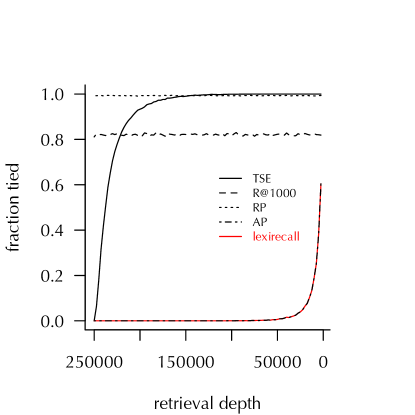
Figure 6. Fraction tied rankings as retrieval depth $\tilde{n}$ decreases for $n=250,000$ and 25 requests. For each query, we selected $m\sim U(5,50)$ relevant items. This figure best rendered in color.

5.2. Lexicographic Recall

We can address the lack of sensitivity of $\operatorname{TSE}$ by turning to recent work on preference-based evaluation (Diaz and Ferraro, 2022; Clarke et al., 2023). As mentioned earlier, in many evaluation scenarios, our objective is to compute $\pi\succ\pi^{\prime}$. In metric-based evaluation, we compute this preference by first computing the value of an evaluation metric for each ranking. That is,

(8) $$\mu(\pi)>\mu(\pi^{\prime})\implies\pi\succ\pi^{\prime}$$

Preference-based evaluation (Diaz and Ferraro, 2022) is a quantitative evaluation method that directly computes the preference between two rankings $\pi$ and $\pi^{\prime}$ without first computing an evaluation metric.

Diaz and Ferraro (2022) show that preference-based evaluation can achieve much higher statistical sensitivity compared to standard metric-based evaluation.

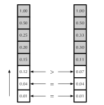
Figure 7. Lexicographic relation between two sorted vectors with the same dimension. In leximin ordering, we compare pairs of elements from the bottom up and define the preference between vectors based on the first difference in values. In this example, the last element in both vectors is $0.01$ and the second to last element is $0.04$ in both. The third to last elements differ and we say that we prefer the ranking on the left because $0.12>0.07$.

We can convert $\operatorname{TSE}$ into a much more sensitive preference-based evaluation by returning to our discussion of fairness and robustness. In the context of social choice theory, the number of ties in Rawlsian fairness can be addressed by adopting a recursive procedure known as leximin, originally proposed by Sen (1970).

Consider the problem of distributing a resource to $m$ individuals, in our case searchers or providers. Further consider two different allocations $x$ and $y$ represented by two $m\times 1$ vectors where $x_{i}$ is the amount of resource allocated to the $i$th highest ranked individual, similarly for $y$. In other words, $x$ and $y$ are the resource allocations in decreasing order. Given these two allocations, we begin by inspecting the allocation to the lowest-ranked items, as we did with Rawlsian fairness. If $x_{m}>y_{m}$, then the bottom-ranked item of $x$ is better off and $x\succ y$; if $x_{m}<y_{m}$, then the bottom-ranked item of $y$ is better off and $x\prec y$; otherwise, the bottom-ranked items are equally well-off and we inspect the position of the next lowest item, $m-1$. If $x_{m-1}>y_{m-1}$, then we say $x\succ y$; if $x_{m-1}>y_{m-1}$, then we say $x\prec y$; otherwise, we inspect the position of the next lowest item $m-2$. We continue this procedure until we return a preference or, if we exhaust all $m$ positions, we say that we are indifferent between the two rankings. Formally,

(9) $$x\succ_{\text{leximin}}y\leftrightarrow x_{i}>y_{i}$$

where $i=\max\{j\in[1\mathrel{{.}\,{.}}\nobreak m]:x_{i}\neq y_{j}\}$. We show a example of this process in Figure 7. This way of comparing rankings generates a total lexicographic ordering over vectors of the same dimensionality and is often used in the fairness literature to address ties when adopting Rawls’ difference principle.

We can use leximin to define the lexicographic recall or lexirecall preference between $\pi$ and $\pi^{\prime}$. For a fixed request and ranking $\pi$, let $\varrho$ be the $m^{+}\times 1$ vector of metric values for $\mathcal{U}$ sorted in decreasing order. In other words, $\varrho_{i}=\mu(\pi,u^{i})$, where $u^{i}$ is the user with the $i$th-highest metric value. We define $\varrho^{\prime}$ equivalently for $\pi^{\prime}$. Lexicographic recall is defined as,

(10) $$\pi\succ_{\text{LR}}\pi^{\prime}\leftrightarrow\varrho\succ_{\text{leximin}}\varrho^{\prime}$$

Using lexirecall, we can define a ordering over unique rankings, which addresses the ties observed in $\operatorname{TSE}$.

Although operating over $\mathcal{U}$ grounds our evaluation in possible user information needs, scoring and ranking $m^{+}$ subsets of $\mathcal{R}$ can be computationally intractable. So, just as we demonstrated that we only need to inspect the position of the last relevant item to compute $\succ_{\text{WC}}$, we can demonstrate that we only need to compare the rank positions of the relevant items to compute $\pi\succ_{\text{LR}}\pi^{\prime}$ (proof in Appendix B.2) and, therefore,

(11) $$\pi\succ_{\text{LR}}\pi^{\prime}\leftrightarrow p_{i}<p^{\prime}_{i}$$

where $i=\max\{j\in[1\mathrel{{.}\,{.}}\nobreak m]:p_{i}\neq p^{\prime}_{j}\}$. Moreover, although defined as a searcher-oriented metric, we can also demonstrate that this results in provider leximin as well (proof in Appendix B.2),

We can better understand lexirecall by returning to our discussion of robustness in Section 4. While $\operatorname{TSE}$ provided one way to distinguish robustness of two rankings, it is very insensitive and unlikely to be of practical use. In order to address this, we adopted leximin, a well-studied method for addressing insensitivity in applying Rawls’ difference principle. That said, lexirecall is still a measure of robustness. A lexirecall preference is simply claiming that one ranking is more fair or more robust than another. Over a population of requests, then, we can compute the probability that one system’s rankings are fairer or more robust than another.

5.3. Sensitivity of Lexicographic Recall

We can demonstrate the higher sensitivity of lexirecall through simulation and analysis of the total space of permutations. In Figure 6, we demonstrated that, for a set of random paired rankings, the number of ties was high for traditional metrics and grew quickly for $\operatorname{TSE}$ as the cutoff $\tilde{n}$ decreased. Figure 6 also includes lexirecall, which exhibits substantially fewer ties than traditional metrics and $\operatorname{TSE}$.

Independent of simulation, we are also interested in the probability of a tie over for randomly sampled pairs of complete rankings $\pi,\pi^{\prime}\in S_{n}$ (i.e. $\tilde{n}=n$). We can derive these probabilities (see Appendix D) as functions of $m$, $n$, and any parameters of the metric (e.g. $k$),

$$\text{Pr}(\pi=_{\operatorname{TSE}}\pi^{\prime}) ={n\choose m}^{-2}\sum_{i=m}^{n}{i-1\choose m-1}^{2}$$

$$\text{Pr}(\pi=_{\text{R}_{k}}\pi^{\prime}) ={n\choose m}^{-2}\sum_{i=0}^{m}{{k\choose i}^{2}{n-k\choose m-i}^{2}}$$

$$\text{Pr}(\pi=_{\text{RP}}\pi^{\prime}) ={n\choose m}^{-2}\sum_{i=0}^{m}{{m\choose i}^{2}{n-m\choose m-i}^{2}}$$

$$\text{Pr}(\pi=_{\text{LR}}\pi^{\prime}) =\frac{m!(n-m)!}{n!}$$

To better understand the relationship between these probabilities, we display probabilities of ties for several retrieval depths in Table 3. Although Figure 6 demonstrated that $\operatorname{TSE}$ exhibited poor sensitivity when $\tilde{n}<n$, it is much more sensitive for complete rankings, in part because random complete rankings are less likely to share $p_{m}$ than imputed rankings. Both traditional recall metrics exhibit many more ties, especially as the retrieval depth grows. Amongst methods, lexirecall and AP demonstrate the few or no ties across corpus sizes. Table 4 presents the same results for varying numbers of relevant items. The results are consist with Table 3, where traditional recall metrics exhibit a large number of ties, which decreases slowly with the number of relevant items. By comparison, $\operatorname{TSE}$, lexirecall, and AP show higher sensitivity with a negligible number of ties.

Table 3. Probability of a metric tie $\text{Pr}(\pi=_{\mu}\pi^{\prime})$ for randomly sampled permutations and $m=10$.

$n$	$\operatorname{TSE}$	$\text{R}_{1000}$	RP	AP	LR
$10^{3}$	0.005	1.000	0.825	0.000	0.000
$10^{4}$	0.001	0.313	0.980	0.000	0.000
$10^{5}$	0.000	0.826	0.998	0.000	0.000
$10^{6}$	0.000	0.980	1.000	0.000	0.000

Table 4. Probability of a metric tie $\text{Pr}(\pi=_{\mu}\pi^{\prime})$ for randomly sampled permutations and $n=10^{6}$.

$m$	$\operatorname{TSE}$	$\text{R}_{1000}$	RP	AP	LR
1	0.000	0.998	1.000	0.000	0.000
5	0.000	0.990	1.000	0.000	0.000
10	0.000	0.981	1.000	0.000	0.000
25	0.000	0.952	0.999	0.000	0.000
50	0.000	0.907	0.995	0.000	0.000

6. Empirical Analysis

In this section, we empirically assess lexirecall with respect to the associated empirical desiderata from Section 2.4: 1 correlation with existing metrics, 2 ability to distinguish between rankings, 3 ability to distinguish between systems, and 4 robustness to missing labels.

6.1. Methods and Materials

6.1.1. Data

We evaluated retrieval runs across a variety of conditions (Table 5). For each dataset, we have a set of evaluation requests and associated relevance judgments. In addition, each dataset involved a number of competing systems, each of which produced a ranking for every request. All datasets were downloaded from NIST.

In order to demonstrate results for different retrieval depths, we categorized datasets as deep ($\tilde{n}>1000$), standard ($\tilde{n}\in(100\mathrel{{.}\,{.}}\nobreak 1000]$), or shallow ($\tilde{n}\leq 100$).

Table 5. Datasets used in empirical analysis. Runs submitted to the associated TREC track. Tracks labeled according to the depth of runs: deep ($\tilde{n}>1000$), standard ($\tilde{n}\in(100\mathrel{{.}\,{.}}\nobreak 1000]$), shallow ($\tilde{n}\leq 100$).

	requests	runs	rel/request	docs/request	depth
legal (2006)	39	34	110.85	4835.07	deep
legal (2007)	43	68	101.023	22240.30	deep
core (2017)	50	75	180.04	8853.11	deep
core (2018)	50	72	78.96	7102.61	deep
deep-docs (2019)	43	38	153.42	623.77	standard
deep-docs (2020)	45	64	39.27	99.55	shallow
deep-docs (2021)	57	66	189.63	98.83	shallow
deep-pass (2019)	43	37	95.40	892.51	standard
deep-pass (2020)	54	59	66.78	978.01	standard
deep-pass (2021)	53	63	191.96	99.95	shallow
web (2009)	50	48	129.98	925.31	standard
web (2010)	48	32	187.63	7013.21	deep
web (2011)	50	61	167.56	8325.07	deep
web (2012)	50	48	187.36	6719.53	deep
web (2013)	50	61	182.42	7174.38	deep
web (2014)	50	30	212.58	6313.98	deep
robust (2004)	249	110	69.93	913.82	standard

6.1.2. Evaluation Methods

We computed lexirecall using pessimistic imputation. We compare LR with two traditional recall metrics ($\text{R}_{1000}$ and RP) and two metrics that combine recall and precision (AP and $\mathrm{NDCG}$). Definitions for metrics can be found in Section 2. An implementation can be found at https://github.com/diazf/pref_eval.

6.2. Results

6.2.1. Agreement with Existing Metrics

To understand the similarity of lexirecall and traditional metrics, we measured its preference agreement with traditional metrics. Specifically, given an observed a metric difference, $\mu(\pi)\neq\mu(\pi^{\prime})$, for a traditional metric in our datasets, we computed how often lexirecall agreed with the ordering of $\pi$ and $\pi^{\prime}$,

$$\frac{\sum_{\pi,\pi^{\prime}\in\tilde{S}_{n}}\text{I}\left(\pi\succ_{\mu}\pi^{\prime}\land\pi\succ_{\text{LR}}\pi^{\prime}\right)}{\sum_{\pi,\pi^{\prime}\in\tilde{S}_{n}}\text{I}\left(\pi\succ_{\mu}\pi^{\prime}\right)}$$

where $\tilde{S}_{n}$ is the set of rankings in our dataset. We present results in Figure 8. For reference, we include high precision metrics $\mathrm{RR}$ and $\mathrm{NDCG}_{10}$, which expectedly have the weakest agreement with lexirecall across all retrieval depths. Similarly, across all depths, we observed highest sign agreement with $\text{R}_{1000}$, indicating an alignment between lexirecall and traditional notions of recall. Note that in the standard and shallow conditions, where $\tilde{n}\leq 1000$, if there is a difference in $\text{R}_{1000}$, then there is a difference in lexirecall due to pessimistic imputation; the converse is not true since lexirecall can distinguish rankings that are tied under $\text{R}_{1000}$. The agreement with $\mathrm{NDCG}$ increases to match that of $\text{R}_{1000}$ with increased depth, perhaps due to the weaker position discounting in NDCG and higher likelihood of including a value based on the lowest ranked relevant item as depth increases (see Section 4.3). Both RP and AP show comparable agreement higher relative to $\mathrm{RR}$ and $\mathrm{NDCG}_{10}$.

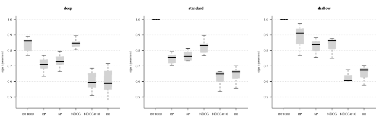
Figure 8. Agreement between lexirecall and traditional metrics over rankings $\pi,\pi^{\prime}$ in TREC datasets. Fraction of ranking pairs where the lexirecall preference agrees with the sign of the metric difference.

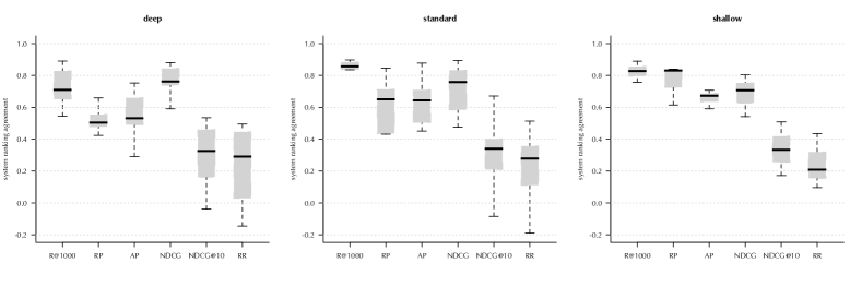
Figure 9. Agreement of TREC system ranking between lexirecall and traditional metrics using Kendall’s $\tau$.

Figure 9 shows the agreement between the ranking of systems by lexirecall and traditional metrics for each dataset, as measured by Kendall’s $\tau$. We aggregated per-query lexirecall system ordering using MC4 (Dwork et al., 2001), as suggested by earlier work in preference-based evaluation (Diaz and Ferraro, 2022). The results are largely consistent with Figure 8. We do not observe perfect correlation with $\text{R}_{1000}$ as we did Figure 8 because 1 scalar $\text{R}_{1000}$ values introduce noise and 2 aggregated lexirecall includes preferences when $\text{R}_{1000}$ is tied. Nevertheless, the agreement is still high relative to other metrics.

6.2.2. Detection of Difference Between Rankings

In Section 5.3, we observed that, for pairs of rankings $\pi,\pi^{\prime}\in S_{n}$ sampled uniformly at random, lexirecall resulted in fewer ties than RP and $\text{R}_{1000}$. Figure 10 presents the empirical fraction of ties when sampling from rankings in our dataset (i.e. $\tilde{S}_{n}$). First, consider traditional recall metrics $\text{R}_{1000}$ and RP. The empirical fraction of ties is substantially lower than suggested by Figure 6 (different $\tilde{n}$) and Table 3 (different $n$). This can be explained by the concentration of relevant items in the top positions $\tilde{S}_{n}$ compared to $S_{n}$, resulting in fewer ties. That said, the fraction of ties for both of these metrics is substantially higher than observed for lexirecall, something consistent with results in Section 4.3. Although AP and $\mathrm{NDCG}$ capture both precision and recall valance, we can see that lexirecall is comparable in fraction of ties.

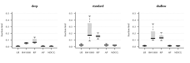
Figure 10. Fraction of tied comparisons of rankings $\pi,\pi^{\prime}$ in TREC datasets.

6.2.3. Statistical Sensitivity

We are also interested in ability of lexirecall to detect statistical differences between pairs of runs (i.e. sets of rankings generated by a single system for a shared set of queries). To do so, we adopted Sakai’s method of measuring the discriminative power of a metric (Sakai, 2014). This approach measures the fraction of pairs of systems that the method detects statistical differences with $p<0.05$. We use two methods to compute $p$-values. In the first, we compute a standard statistical test and, correcting for multiple comparisons, measure the fraction of $p$-values below $0.05$. For lexirecall, we adopt a binomial test since we have binary outcomes. For other metrics, we adopt a Student’s $t$-test, as recommended in the literature (Smucker et al., 2007). We also conducted experiments using incorrect-but-consistent statistical tests with similar outcomes. In order to correct for multiple comparisons for all tests, we use the conservative Holm-Bonferroni method (Boytsov et al., 2013). Our second method of computing $p$-values uses Tukey’s honestly significant difference (HSD) test as proposed by Carterette (2012). This method is considered a more appropriate approach to addressing multiple comparisons compared to our first approach. The goal of this analysis is to understand the statistical sensitivity of lexirecall compared to other recall-oriented metrics, while presenting non-recall metrics for reference.

We present the results of this analysis in Figure 11. When using standard tests (Figure 11(a)), lexirecall is slightly better at detecting significant differences compared to existing recall metrics at deeper retrievals. We can refine this analysis by inspecting the HSD results (Figure 11(b)). In this case, the sensitivity of lexirecall manifests more strongly, clearly more discriminative than existing recall metrics for deep retrievals, although losing this power as retrieval depth decreases. This is consistent with previous observations for preference-based evaluation (Diaz and Ferraro, 2022).

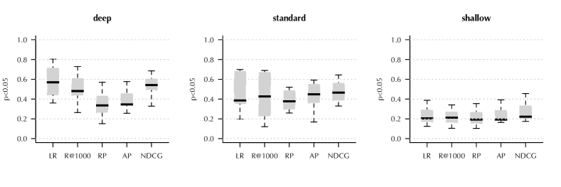
(a) Paired Test

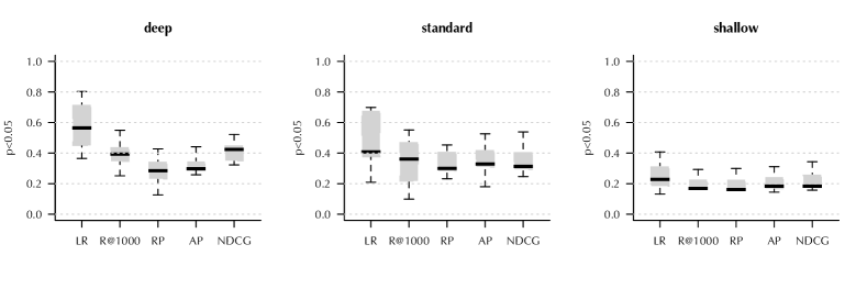
(b) HSD

Figure 11. Statistical sensitivity. Fraction of run pairs where we observe a statistically significant difference (i.e. $p<0.05$).

6.2.4. Label Degradation

Effective evaluation methods are robust to missing relevance labels. In this analysis, we held the number of queries fixed and randomly removed a fraction of relevant items per query, leaving at least one relevant item per query. We consider two ways to sample items to remove. First, we uniformly sample from all relevant items $\mathcal{R}$ to remove. Second, we sample from $\mathcal{R}$ based on the number of rankings in $\tilde{S}_{n}$ the item appears in. We expect metrics to degrade in performance more quickly when removing ‘popular’ items. We present results for the effect of label degradation on the fraction of ties (we expect more ties with fewer labels) and preference agreement with full data (we expect lower agreement with fewer labels). As with the previous section, the goal of this analysis is to compare lexirecall to other recall-oriented metrics, while presenting non-recall metrics for reference.

In terms of fraction of ties (Figure 12), lexirecall degrades comparably to metrics like AP and $\mathrm{NDCG}$ and substantially more gracefully compared to existing recall metrics $\text{R}_{1000}$ and RP. While the importance of relevance labels for recall-oriented evaluation is important, this result suggests that existing metrics are extremely brittle when labels are missing. All methods observed more ties at shallower retrieval depths with degradation more pronounced for traditional recall-oriented metrics.

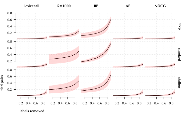
(a) Uniform Label Degradation

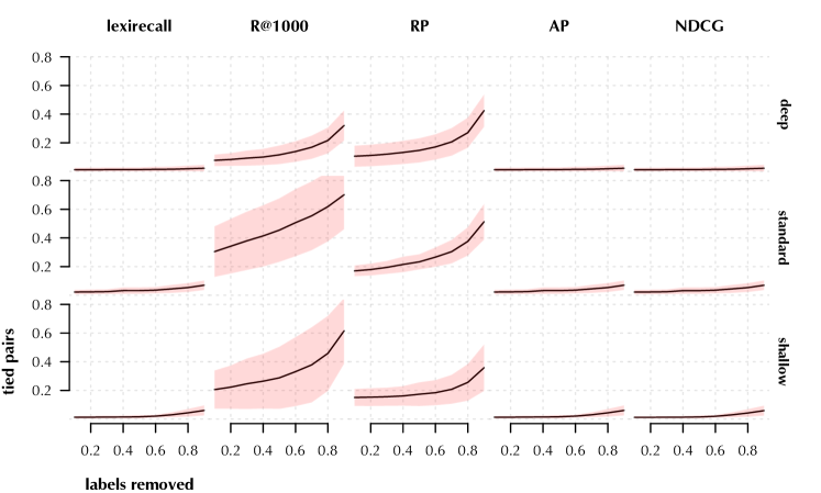
(b) Ranking Frequency Label Degradation

Figure 12. Number of ties as labels removed. For each query, we removed a fraction of items from $\mathcal{R}$ and counted the number of tied rankings. Relevant items were either (12(a)) sampled uniformly at random or (12(b)) weighted by their frequency in amongst the submitted rankings $\tilde{S}_{n}$. Average over ten samples.

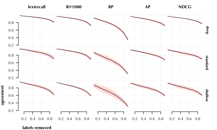
(a) Uniform Label Degradation

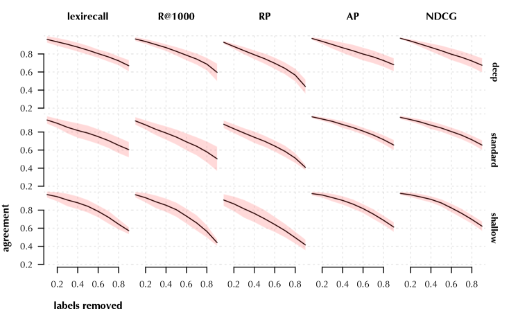
(b) Ranking Frequency Label Degradation

Figure 13. Preference agreement between metric based on degraded labels and complete labels. For each query, we removed a fraction of items from $\mathcal{R}$ and measured the fraction of preferences $\succ_{\mu}$ based on the incomplete relevance judgments that agreed with the preference when using the complete set of relevant items. Relevant items were either (13(a)) sampled uniformly at random or (13(b)) weighted by their frequency in amongst the submitted rankings $\tilde{S}_{n}$. Average over ten samples.

In terms of agreement with preferences based on full data (Figure 13), lexirecall again degrades comparably to AP and $\mathrm{NDCG}$ while RP is much more sensitive across degradation levels. On the other hand, $\text{R}_{1000}$ behaves similar to lexirecall when preserving most labels, but, for drastically sparse labels, the agreement drops. We again see slightly worse degradations with shallower retrieval depths across all metrics. RP in particular demonstrates significantly worse degradation compared to all metrics, while $\text{R}_{1000}$ shows worse degradation when removing relevant items based on ranking frequency.

7. Discussion

We begin our discussion by returning to the desiderata in Section 2.4. We originally sought to define and understand recall from a more formal grounding, allowing us to draw connections to recent literature in fairness and robustness, supporting our first desideratum. Moreover, our definition of recall orientation both directly implied the appropriate recall metric and differentiated it from existing metrics, supporting our second desideratum. Finally, our empirical analysis demonstrated that lexirecall captures many of the properties of existing metrics, while being substantially more sensitive and robust to missing labels, supporting our remaining desideratum. Collectively, we find strong support for investigating lexirecall as a method for assessing our robustness perspective of recall.

In light of our conceptual, theoretical, and empirical analysis, we can make a number of other observations about recall, robustness, and lexicographic evaluation.

7.1. Recall

7.1.1. Labeling

Although lexirecall appears more robust to missing labels than existing recall-oriented metrics, the performance of recall and robustness evaluation depends critically on having comprehensive relevance labels. While time-consuming, we believe that, in order to develop robust and fair systems, new techniques for expanding labeled sets for recall evaluation are necessary. Initiatives like TREC adopt pooling as a strategy to achieve more complete judgments. Unfortunately, in situations where relevance is derived from behavioral feedback (e.g. (Kelly and Teevan, 2003; Chandar et al., 2020)), comprehensiveness of relevance is often not the focus. Moreover, the transience of information needs in production environments makes reliable detection of $\mathcal{R}$ an open problem. This situation is exacerbated in recommender system environments where judgments, while often highly personalized and based on psychological relevance, can be extremely incomplete (see (Herlocker et al., 2004) for a discussion).

7.1.2. Depth Considerations for Recall-Oriented Evaluation

All of our recall-oriented evaluations (e.g. lexirecall, RP, $\text{R}_{1000}$) suffer when operating within a shallow retrieval environment. We recommend that, especially for recall-oriented evaluation, retrieval depths be high, regardless of the specific evaluation method. Moreover, as labels become sparser, both RP and $\text{R}_{1000}$ show substantially more ties (Figure 12) and poor robustness (Figure 13). We recommend that, for shallow retrieval with sparse labels, RP should be avoided altogether.

7.2. Robustness

7.2.1. Number of Ties and Metric-Based Evaluation

The high number of ties from RP and $\text{R}_{1000}$ arises when collapsing all permutations that share the same recall value. Top-heavy recall-level metrics that have nonzero weight over all relevant items effectively encode the $n\choose m$ permutations onto the real line. We should expect more ties and lower statistical sensitivity for metrics that have low cutoffs (e.g. $\tilde{n}<100$). This includes $\mathrm{RR}$ and variants of top-heavy recall-level metrics with rank cutoffs (e.g. $\mathrm{NDCG}_{10}$). Even for top-heavy recall-level metrics, we expect ties if $e(i)\approx 0$ for unretrieved items or if the numerical precision limits the ability to represent all $n\choose m$ positions of relevant items. Because of their top-heaviness, these ties are more likely to occur for differences at the lower ranks, precisely the positions worst-case performance emphasizes. As a result, even though some top-heavy metrics may theoretically include worst-case performance, they will not emphasize it in the metric value.

7.2.2. Mixed Orientation Metrics

We saw agreement between lexirecall and $\mathrm{NDCG}$, even though the latter captures precision orientation (Figure 3). In Section 4.3, we explained that this may be due to either the inclusion of $p_{m}$ in top-heavy recall-level metric computation (Equation 1) or because of structural dependencies between rank positions of $p_{i}$ and $p_{j}$. Alternatively, since we observed strong empirical agreement between lexirecall and $\mathrm{NDCG}$, the position of the last ranked relevant item may be predictable because of systematic behavior in the model. For example, for many scenarios, performance higher in the ranking may be predictive of worst-case performance. Even if this is case for many systems or domains, we caution against presuming that performance at the top of the ranking is predictive of worst-case performance. If the worst-case performance is systematic and amongst smaller-sized groups (i.e. those unlikely to appear at the top), then the performance will not be well-predicted by larger, systematically-higher ranked items from dominant groups. We recommend lexirecall to detect worst-case performance in isolation of other criteria (e.g. precision).

7.2.3. A Comment on Graded Metrics

Although we have focused on binary topical relevance, many retrieval scenarios use graded or ordinal relevance. Consider relevance labels represented as an ordinal scale, where higher grades reflect a higher probability of satisfying the information need according to the rater’s subjective opinion.

Under such a grading scheme, an item labeled with the minimum grade has a probability of relevance of $0$ (i.e. no user would ever find the item relevant) and an item labeled with the maximum grade has a probability of relevance of $1-\epsilon$ (i.e. almost every user would find the item relevant).

We can determine grades that reflect the probability of relevance through 1 labeling instructions (e.g. ‘an item with a high grade should satisfy many users; an item with a medium grade should satisfy some users; an item with a low grade should satisfy few users’), 2 voting schemes (Gordon et al., 2021), or 3 aggregated behavioral data (e.g., clickthrough rate) (Zheng et al., 2010). No matter how grades are determined, for a fixed request, a searcher with a less popular intent may not be satisfied by an item relevant to a more popular intent. This implies that notions of optimality in graded retrieval evaluation (i.e. that higher grades should be ranked above lower grades) explicitly values dominant group intents over minority intents. From the perspective of robustness, this means that, for graded judgments, we should consider $\mathcal{R}$ to include all items with a non-zero chance of satisfying a searcher. This is precisely the approach adopted for $\operatorname{TSE}$ and lexirecall.

7.2.4. Robustness of Optimal Rankings

In the case of binary relevance, Robertson (1977)’s Probability Ranking Principle suggests that an optimal ranking will place all relevant items above nonrelevant items. If $S_{n}^{*}$ is the set of optimal permutations, then it consists of permutations that rank all of the items in $\mathcal{R}$ above $\mathcal{D}-\mathcal{R}$. Traditional information retrieval methods have largely been deterministic insofar as, given a request, they always return a fixed $\pi\in S_{n}$. The optimal deterministic ranker, then, is any ranker that selects a fixed $\pi\in S_{n}^{*}$ and, therefore, for any optimal deterministic ranker, the worst-case performance is $e(m)$.

The situation changes if we consider stochastic rankers (Radlinski and Joachims, 2007; Bruch et al., 2020; Diaz et al., 2020; Singh and Joachims, 2018; Oosterhuis and de Rijke, 2020), systems that, in response to a request, sample a ranking $\pi$ from some distribution over $S_{n}$. Such systems have been proposed in the context of online learning (Radlinski and Joachims, 2007) and fair ranking (Diaz et al., 2020). An optimal stochastic ranker would, in response to a request, uniformly sample a ranking from $S_{n}^{*}$.

We can show that the worst-case expected performance of the optimal stochastic ranker is better than the worst-case expected performance for any optimal deterministic ranker,

$$\min_{u\in\mathcal{U}}\mathbb{E}_{\pi\sim S_{n}^{*}}\left[\mu(\pi,u)\right] \geq\min_{u\in\mathcal{U}}\mu(\pi^{*},u),\forall\pi^{*}\in S_{n}^{*}$$

We present a proof in Appendix C.

Figure 14 displays the difference in worst-case performance between optimal deterministic and stochastic rankings for $m\in[1\mathrel{{.}\,{.}}\nobreak 25]$. This result provides evidence from a robustness perspective that information retrieval system design should explore the design space of stochastic rankers.

Figure 14. Worst-case performance of optimal deterministic and stochastic rankings for $m\in[1\mathrel{{.}\,{.}}\nobreak 25]$.

7.3. Lexicographic Evaluation

7.3.1. Beyond Recall

Worst-case performance directly influenced the design of lexirecall. Using binary relevance was based on possible information needs; adopting leximin was based on focusing on the worst-off individuals. This same formalism allows us to introduce a notion of lexicographic precision or lexiprecision, defined using the leximax relation. The idea is identical to leximin, except that we start from the top of the ranking.

Just as lexirecall proceeds from the lowest-ranked relevant item upward, lexiprecision proceeds from the highest-ranked relevant item downward. While we can motivate lexiprecision from best-case analysis, we can also use it as a version of the $\mathrm{RR}$ that more gracefully deals with tied rankings. To see why, we can observe that, whenever $\mathrm{RR}$ detects a difference in performance, lexiprecision will agree,

$$\mathrm{RR}(\pi,\mathcal{R}) >\mathrm{RR}(\pi^{\prime},\mathcal{R})\rightarrow\pi\succ_{\text{LP}}\pi^{\prime}$$

When there is a tie in $\mathrm{RR}$ between two rankings, lexiprecision falls back to lower ranked relevant items. Beyond high precision, we believe criteria such as diversity, group fairness, and graded judgments can also be incorporated into lexicographic retrieval.

7.3.2. Recovering an Evaluation Metric

In contrast with preference-based evaluation like lexirecall, metric-based evaluation can be performed efficiently for each ranking independently, moving the complexity from $O(|\tilde{S}_{n}|\log|\tilde{S}_{n}|)$ to $O(|\tilde{S}_{n}|)$. Fortunately, existing results in the computation of leximin point to how to design such a metric.

Yager (1997) demonstrates one can construct a leximin representation of a ranking such that $\text{leximin}(x)>\text{leximin}(y)\leftrightarrow x\succ_{\text{leximin}}y$. Specifically, if $x$ is a $m\times 1$ allocation vector sorted in decreasing order,

(12) $$\text{leximin}(x) =\sum_{i=1}^{m}w_{i}x_{i}$$

where $w$ is a bottom-heavy weight vector such that $w_{1}\ll w_{2}\ll\ldots\ll w_{m}$. In our situation, a system ‘allocates’ exposure but, because $e(p_{i})$ is a monotonically decreasing function of $p_{i}$, we only need to compare the rank positions $p$. As such, we can define our allocation vectors as $x_{i}=\frac{n-p_{i}}{n}$. We can use this to define the recall level weight vector $w$ as,

$$w_{i} =\begin{cases}\frac{\Delta^{m-1}}{(1+\Delta)^{m-1}}&i=1\\ \frac{\Delta^{m-i}}{(1+\Delta)^{m+1-i}}&i>1\end{cases}$$

where $\Delta=(n+\epsilon)^{-1}$ and $\epsilon\in(0,1)$ is a free parameter.

We can then define metric lexirecall as,

$$\text{LR}(p) =\text{leximin}(x)$$

$$\propto-\sum_{i=1}^{m}w_{i}p_{i}$$

We can then compare rankings directly using $\text{leximin}(p)$. Since $\sum_{i}w_{i}=1$, this can be interpreted as the bottom-heavy weighted average of the positions of relevant items. We contrast this with uniform weighting found in the recall error metric (Rocchio, 1964) or top-heavy weighting found in precision-oriented metrics.

While providing interesting theoretical connection to existing top-heavy recall-level metrics, in practice, due to the large values of $n$ and $p_{i}$, computing the metric lexirecall can suffer from numerical precision issues. When $n$ is unknown—for example in dynamic or extremely large corpora—metric lexirecall cannot be calculated at all. In these situations, computing lexirecall is feasible due to our imputation procedure and the fact that we only care about relative positions.

7.3.3. Optimization

Although our focus has been on evaluation, optimizing for lexicographic criteria may be an alternative method for designing recall-oriented algorithms, for example for technology-assisted review or candidate generation. One way to accomplish this is to optimize for metric lexirecall discussed in the previous section. Since learning to rank methods often optimize for functions of positions of relevant items (e.g. (Qin et al., 2010)), standard approaches may suffice. Alternatively, in Section 7.2.4, we observed that optimal stochastic rankers outperformed optimal deterministic rankers in terms of worst-case performance. This suggests that stochastic ranking techniques similar to those developed in the context of other fairness notions (e.g. (Diaz et al., 2020)) can be used for recall-oriented tasks.

8. Related Work

8.1. Recall

Given its history in information retrieval, recall, like precision, has several different ways of being measured. In classic set-based retrieval, recall is measured as the fraction of relevant items in the retrieved set. Recent work on set-based recall prove that, unlike many rank-based metrics, it is an interval scale (Ferrante et al., 2017, 2019, 2020, 2021). In technology-assisted review, a system-determined cutoff can be used to compute set-based recall metrics (Cormack and Grossman, 2016; Lewis et al., 2021). However, most ranked retrieval systems do not provide such a cutoff, requiring ranked recall metrics. Many of these metrics compute functions of the rank positions of the relevant items. For example, Rocchio (1964) proposed recall error, a metric based on the average rank of the relevant items, which Robertson (1969) proved was equal to Swets’ A measure (Swets, 1969). Zou and Kanoulas (2020), in the context of technology-assisted review, measure recall as the position of the lowest ranked relevant item, which is identical to our TSE metric. Unfortunately, as we noted, for very large collections, the average or last rank can be sensitive to outliers. In response, Magdy and Jones (2010a) introduced a correction for this recall error to address this instability.

As mentioned in Section 1, rank-based metrics are often compared as more or less ‘recall-oriented’ without a formal description of what that means (Kazai and Lalmas, 2006; Montazeralghaem et al., 2020; Dai et al., 2017; Mohammad et al., 2018; Li et al., 2014; Diaz, 2015). While there has been work on theoretical properties of metric properties in general (Moffat, 2013; Busin and Mizzaro, 2013; Ferrante et al., 2019), there has not been a formal treatment of what it means for a metric to be recall-oriented. As such, our discussion in Section 3.1 contributes to the literature on formally understanding metrics.

Despite its persistance in evaluation, recall has been a contentious concept. Cooper (1968) argued that recall-orientation is inappropriate because user search satisfaction depends on the number of items the user is looking for, which may be fewer than all of the relevant items. This is an observation noted by several other authors (Moffat, 2013; Ferrante et al., 2015). Zobel et al. (2009) refute several justifications for recall: persistence (the depth a user is willing to browse), cardinality (the number of relevant items found), coverage (the number of user intents covered), density (the rank-locality of relevant items), and totality (the retrieval of all relevant items). In each of these cases, they note that recall is either the inappropriate measure or that the justification is unfounded.

8.2. Robustness

In the context of information retrieval, robustness has often focused on performance across unique queries. For example, the TREC Robust track emphasized evaluation on difficult queries (Voorhees, 2004). Risk-based robust evaluation seeks to ensure that performance improvements are robust across all queries with respect to a baseline (Wang et al., 2012; Collins-Thompson et al., 2013). Meanwhile, Goren et al. (2018) propose robustness in light of adversarial document manipulation. In the context of recommender systems, robustness has analogously focused on cross-user robustness (Xu et al., 2020; Wen et al., 2022) and adversarial content providers (Mobasher et al., 2007). From a simulation perspective, Ovaisi et al. (2022) developed a system to consider system robustness in light of distribution shift. Finally, Valcarce et al. (2020) evaluate the robustness of evaluation metrics themselves.

Although these earlier dimensions of robustness are important, they differ from our focus on robust performance across possible users issuing the same request. Mehrotra et al. (2017), in the context of auditing a search engine, introduce the concept of ‘differential satisfaction’, the difference in performance for different users issuing the same query. This is close to the notion of robustness proposed by Memarrast et al. (2021), who consider a worst-case user for whom relevant items have a marginal distribution of features that matches the distribution in the full training set. While similar to our notion of robustness, we consider the full set of worst-case situations, including those that do not match the training data. Unlike two-sided worst-case fairness (Do et al., 2021), we study these properties within a ranking as opposed to across rankings.

Finally, in the context of fair ranking, robustness has focused on the equal exposure of content providers (e.g. document authors, item creators) (Biega et al., 2018; Singh and Joachims, 2018; Diaz et al., 2020; Ekstrand et al., 2022). Mathematically, this can look like the $\ell_{2}$ norm of the exposure vector (Diaz et al., 2020) which is different from the minimum exposure we adopt for TSE based on Rawls’ difference principle (Rawls, 2001). The focus on the Rawls’ difference principle, in turn, allows us to adopt more sensitive, lexicographic comparison (Sen, 1970). Understanding the appropriate definition of fairness depends on the particular sociotechnical context (Barocas et al., 2019). That said, the expected exposure metric for a deterministic ranker (i.e., those we consider in our experiments) will be equivalent to classic precision metrics such as NDCG and RBP (Diaz et al., 2020, Equation 2) rather than recall metrics, as we focus on.

8.3. Preference-Based Evaluation

Although the original presentation of preference-based evaluation focused on aggregating a population of position-based preferences (Diaz and Ferraro, 2022), this is not the first work study pairwise preferences or partial orders of rankings. For example, we can contrast our work with evaluation using item preferences (Clarke et al., 2021, 2020, 2023), which is still a metric-based evaluation but based on pairwise preferences between items.

(Ferrante et al., 2019) use an explicit ordering of systems in order to analyze existing metrics, including set-based recall metrics. Instead of using an ordering to analyze metrics, we abandon metrics altogether and focus on simply generating an ordering of systems, in this case by lexicographic ordering. This total order may then be amenable to construction of an interval metric (e.g., a linear transform of the position in the ranking of $S_{n}$ by lexirecall).

9. Conclusion

This paper investigated recall, its connection to robust evaluation, and how to effectively measure it through lexicographic evaluation. By providing a clear formal visualization of recall-orientation, we could both directly capture the recall-orientation of existing metrics and recognize a missing ‘basis metric’ for recall. By developing $\operatorname{TSE}$ as the counterpart to $\mathrm{RR}$, we could directly connect recall-orientation to robustness and Rawlsian fairness. This provides a strong motivation—from a fairness perspective—for improving techniques for gathering complete relevance judgments, to ensure the effective computation of recall and, in turn, address potential unfairness. To effectively deploy $\operatorname{TSE}$, we developed lexicographic evaluation and the lexirecall preference-based evaluation method, which we empirically demonstrated was preferable to existing recall metrics. We anticipate that variants of lexicographic evaluation can be applied for other constructs, such as precision. These three themes of recall, robustness, and lexicographic evaluation, while each individually potentially being interesting areas of theoretical analysis, work collectively to substantially improve our understanding of a metric that may be as old as the field of information retrieval: recall.

Appendix A Metric Properties

We can connect our proposed metrics to prior work by leveraging several properties defined in the community. Drawing on fundamental contributions from Moffat (2013), Ferrante et al. (2015), and Amigó et al. (2013), we produced a synthesized list of properties. These properties should be considered descriptive—not prescriptive—since 1 they can be in tension, and 2 there are valid metrics (e.g., high-precision, diversity, fairness) that do not satisfy all of them. Let $\tilde{\pi}$ be a top-$\tilde{n}$ from which we impute a total ranking using pessimistic imputation (Section 2.2).

Consistent with our setup, we assume that the evaluator has access to a set of fixed relevance assessments $\mathcal{R}$ over a fixed corpus $\mathcal{D}$ and pessimistic imputation of a top-$\tilde{n}$ ranking $\tilde{\pi}$. Given a ranking $\pi$, let $y_{i}$ refer to the relevance of $\pi_{i}$. Finally, we assume that the number of unretrieved $n-\tilde{n}$ items is larger than the number of relevant items $m$, which is the case in most retrieval tasks.

1. Monotonicity in retrieval size (Moffat, 2013; Amigó et al., 2013). This property refers to the behavior of $\mu$ as we append items to $\tilde{\pi}$. Following Moffat (2013), a metric is monotonically increasing in retrieval size if it is non-decreasing as $\tilde{n}$ is increased by appending either relevant or nonrelevant items to $\tilde{\pi}$. Following Amigó et al. (2013), a metric is (strictly) monotonically decreasing in nonrelevance if it (strictly) decreases as $\tilde{n}$ is increased by appending nonrelevant items to $\tilde{\pi}$; Amigó et al. (2013) refer to the strict version of this as ‘Confidence’. Note that the Moffat (2013) and Amigó et al. (2013) properties are in tension. For completeness, we refer to a a metric as (strictly) monotonically increasing in relevance if it (strictly) increases as $\tilde{n}$ is increased by appending relevant items to $\tilde{\pi}$.

2. Monotonicity in swapping up (Moffat, 2013; Amigó et al., 2013; Ferrante et al., 2015). A metric is (strictly) monotonically increasing in swapping up if, when $i<j$ and $y_{i}<y_{j}$, we observe a (strictly) monotonic increase in $\mu$ when we swap the documents at positions $i$ and $j$. Ferrante et al. (2015) refers to the non-decreasing property as ‘Swap’. When $j>\tilde{n}$, Moffat (2013) refers to the strictly increasing property as ‘Convergence’ and Ferrante et al. (2015) refers to the non-decreasing property as ‘Replacement’. When $j\leq\tilde{n}$, Moffat (2013) refers to the strictly increasing property as ‘Top-weightedness’. For contiguous swaps (i.e., $j=i+1$), Amigó et al. (2013) refer to the strictly increasing property as ‘Priority’.

3. Concavity in contiguous swap depth (Amigó et al., 2013). A metric is (strictly) concave in contiguous swap depth if, when $i<j$ and $y_{i}<y_{i+1}$ and $y_{j}<y_{j+1}$, swapping $i$ and $i+1$ will lead to a (strictly) larger improvement in $\mu$ compared to swapping $j$ and $j+1$. Amigó et al. (2013) refer this to ‘Deepness’.

4. Suffix Invariance (Amigó et al., 2013). Given two rankings $\pi$ and $\pi^{\prime}$ that have relevant items in same positions in the top-$\tilde{n}$ prefix, a metric is suffix invariant if, no matter the positions of the remaining relevant documents, the metric values will be the same. Amigó et al. (2013) refer this to ‘Deepness Threshold’.

5. Prefix Invariance (Amigó et al., 2013). Given two rankings $\pi$ and $\pi^{\prime}$ that have relevant items in same positions in the bottom-$k$ suffix, a metric is prefix invariant if, no matter the positions of the remaining relevant documents, the metric values will be the same. Amigó et al. (2013) refer this to ‘Closeness Threshold’.

6. Boundedness (Moffat, 2013). A metric is bounded if it is of the form $\mu:S_{n}\times\mathcal{D}^{+}\rightarrow[0,1]$.

7. Localization (Moffat, 2013). A metric is localized if can be computed only with the information in the top-$\tilde{n}$; in other words, the metric value is independent of the positions or number of unretrieved relevant items.

8. Completeness (Moffat, 2013). A metric is complete if it is defined when $m=0$.

9. Realizability (Moffat, 2013). If $m>0$, then the metric can reach its upper bound with a top-$\tilde{n}$ retrieval where $\tilde{n}>0$.

In some cases, we have adopted a property name different from the original to help with clarity. In subsequent sections, we will be demonstrate which of these properties are present for top-heavy recall-level metrics, TSE, and lexirecall.

Several properties were not present in any of our evaluation methods. None of our methods are strictly decreasing in nonrelevance. Amigó et al. (2013) note also that, “[a]s far as we know, current evaluation measures do not consider this aspect.” None of our methods are prefix or suffix invariant. This is largely due to the fact that 1 exposure is strictly monotonically decreasing, and 2 normalization is a function of recall level (and the number of relevant items). As a result, any position-based ‘flatness’ in the computation is missing. None of our methods are guaranteed to be bounded to allow maximal flexibility in our analysis; this also means that none of our methods are guaranteed to be realizable. None of our methods are localized because we explicitly use $m$ and $n$ in pessimistic imputation; while lexirecall does not need $n$, it does still requite $m$.

We summarize the properties for top-heavy recall-level metrics, total search efficiency, and lexirecall in Table 6.

Table 6. Metric Properties. 1: if the second derivative of the exposure function is strictly positive. 2: if normalization function is defined for $m=0$. The properties concavity, boundedness, localization, completeness, and realizability are specific to metric-based evaluation and therefore cannot be analyzed for preference-based evaluation like lexirecall.

	THRL	THRL	$\operatorname{TSE}$	LR
		$z(i,m)>0$
increasing in retrieval size (Moffat, 2013)	$\checkmark$	$\checkmark$	$\checkmark$	$\checkmark$
decreasing in nonrelevance	$\checkmark$	$\checkmark$	$\checkmark$	$\checkmark$
strictly decreasing in nonrelevance (Amigó et al., 2013)
increasing in relevance	$\checkmark$	$\checkmark$	$\checkmark$	$\checkmark$
strictly increasing in relevance		$\checkmark$		$\checkmark$
increasing in swapping up (Ferrante et al., 2015)	$\checkmark$	$\checkmark$	$\checkmark$	$\checkmark$
strictly increasing in swapping up (Moffat, 2013; Amigó et al., 2013)		$\checkmark$
concavity in contiguous swap depth	$\checkmark$	$\checkmark$	$\checkmark$	NA
strict concavity in contiguous swap depth (Amigó et al., 2013)		$\checkmark^{1}$		NA
suffix invariance (Amigó et al., 2013)
prefix invariance (Amigó et al., 2013)
boundedness (Moffat, 2013)				NA
localization (Moffat, 2013)				NA
completeness (Moffat, 2013)	$\checkmark^{2}$	$\checkmark^{2}$	$\checkmark^{2}$	NA
realizability (Moffat, 2013)				NA

A.1. Properties of Top-Heavy Recall-Level Metrics

Let $\mu$ be a top-heavy recall-level metric with exposure function $e$ and normalization function $z$.

Theorem A.1.

$\mu$ is monotonically increasing in retrieval size.

Proof.

Let $\tilde{\pi}^{\prime}$ be $\tilde{\pi}$ with another item appended, with pessimistically imputed rankings $\pi^{\prime}$ and $\pi$. If the new item is nonrelevant, then $\forall i,p_{i}=p^{\prime}_{i}$ and, therefore, $\mu(\pi,\mathcal{R})=\mu(\pi^{\prime},\mathcal{R})$ and $\mu$ is trivially non-decreasing. Next, consider the case where the new item is relevant. This can only happen if $\tilde{\pi}$ includes $\tilde{m}<m$ relevant items. As such, this is equivalent to swapping a relevant item in the imputed ranking $\pi$ from position $n-(m-\tilde{m}-1)$ to position $\tilde{n}+1$. Let $\Delta_{i,j}\mu(\pi,\mathcal{R})$ be the difference in metric value from swapping a relevant item in position $j$ to position $i$.

$$\Delta_{\tilde{n}+1,n-(m-\tilde{m}-1)}\mu(\pi,\mathcal{R}) =\mu(\pi^{\prime},\mathcal{R})-\mu(\pi,\mathcal{R})$$

$$=\sum_{i=1}^{m}e(p^{\prime}_{i})z(i,m)-\sum_{i=1}^{m}e(p_{i})z(i,m)$$

$$=e(p^{\prime}_{\tilde{m}+1})z(\tilde{m}+1,m)-e(p_{\tilde{m}+1})z(\tilde{m}+1,m)$$

(13) $$=z(\tilde{m}+1,m)(e(\tilde{n}+1)-e(n-(m-\tilde{m}-1)))$$

Since $z(i,m)\geq 0$ and $e(\tilde{n}+1)>e(n-(m-\tilde{m}-1))$, we know that Equation 13 will always be non-negative. ∎

Theorem A.2.

$\mu$ is monotonically decreasing in nonrelevance.

Proof.

See the first case in the proof Theorem A.1. ∎

Theorem A.3.

If $z(i,m)$ is (strictly) positive, $\mu$ is (strictly) monotonically increasing in relevance.

Proof.

See the second case in the proof Theorem A.1. Moreover, if $z(i,m)$ is strictly positive, then Equation 13 will always be strictly positive. ∎

Theorem A.4.

If $z(i,m)$ is (strictly) positive, $\mu$ is (strictly) monotonically increasing in swapping up.

Proof.

Given a ranking $\pi\in S_{n}$, let $j$ be the $j$th relevant item and $k<p_{j}$ the position of an arbitrary nonrelevant item ranked above it. Let $\ell$ be the recall level of the first relevant item below position $k$ (i.e., $\ell=\min\{i:p_{i}>k\}$).

$$\Delta_{p_{j},k}\mu(\pi,\mathcal{R}) =z(\ell,m)(e(k)-e(p_{\ell}))+\sum_{i=\ell}^{j-1}z(i+1,m)(e(p_{i})-e(p_{i+1}))$$

Since $z(i,m)\geq 0$ and $e(p^{\prime}_{i})>e(p_{i})$ for $i\in[\ell,j]$, we know that this difference will always be non-negative. Moreover, if $z(i,m)$ is strictly positive, then the difference will always be strictly positive. ∎

Theorem A.5.

If $z(i,m)$ strictly positive and the second derivative of $e$ is (strictly) positive, then $\mu$ is (strictly) concave in contiguous swap depth.

Proof.

Let $\pi,\pi^{\prime}\in S_{n}$ be two rankings whose relevant position vectors differ in one element $j$ (i.e., $\forall i\neq j,p_{i}=p^{\prime}_{i}$) and $p_{j}<p^{\prime}_{j}$. The metric difference for moving the $j$th relevant item up one positions in $\pi$ is,

$$\Delta_{p_{j},p_{j}-1}\mu(\pi,\mathcal{R}) =z(j,m)(e(p_{j}-1)-e(p_{j}))$$

If the second derivative of $e$ is positive, since $p_{j}<p^{\prime}_{j}$,

$$(e(p_{j}-1)-e(p_{j})) \geq(e(p^{\prime}_{j}-1)-e(p^{\prime}_{j}))$$

Moreover, because $z(i,m)>0$,

$$z(j,m)(e(p_{j}-1)-e(p_{j})) \geq z(j,m)(e(p^{\prime}_{j}-1)-e(p^{\prime}_{j}))$$

$$\Delta_{p_{j},p_{j}-1}\mu(\pi,\mathcal{R}) \geq\Delta_{p^{\prime}_{j},p^{\prime}_{j}-1}\mu(\pi,\mathcal{R})$$

Where the inequality is strict if the second derivative of $e$ is strictly positive. ∎

Theorem A.6.

If $z(i,m)$ is defined for $m=0$, then $\mu$ is complete.

Proof.

The only factor in Equation 1 that depends on $m$ is $z$. If it is defined for $m=0$, then $\mu$ is defined as well. ∎

We note that, of the remaining properties, although we cannot prove every top-heavy recall-level metric will satisfy them, there are top-heavy recall-level metrics that do.

A.2. Properties of Total Search Efficiency

Let $\mu$ be TSE with an arbitrary exposure function $e$ and normalization function $z$. Because TSE is a top-heavy recall-level metric, we know that it satisfies all of the properties in Section A.1 except those conditional on $z(i,m)>0$, since $z_{\text{SL}_{3}}(i,m)=0$ when $i<m$.

A.3. Properties of lexirecall

Theorem A.7.

lexirecall is monotonically increasing in retrieval size.

Proof.

Let $\tilde{\pi}^{\prime}$ be $\tilde{\pi}$ with another item appended, with pessimistically imputed rankings $\pi^{\prime}$ and $\pi$. If the new item is nonrelevant, then $\forall i,p_{i}=p^{\prime}_{i}$ and, therefore, $\mu(\pi,\mathcal{R})=\mu(\pi^{\prime},\mathcal{R})$ and lexirecall is trivially non-decreasing. Next, consider the case where the new item is relevant. This can only happen if $\tilde{\pi}$ includes $\tilde{m}<m$ relevant items. As such, this is equivalent to swapping a relevant item in the imputed ranking $\pi$ from position $n-(m-\tilde{m}-1)$ to position $\tilde{n}+1$. Because of pessimistic imputation, the bottom $m-\tilde{m}-1$ relevant items will be tied. However, $p^{\prime}_{m+1}=\tilde{n}+1$ and $p_{m+1}=n-(m-\tilde{m}-1)$. If $m-\tilde{m}<n-\tilde{n}$, then lexirecall will be positive. ∎

Theorem A.8.

lexirecall is monotonically decreasing in nonrelevance.

Proof.

Let $\tilde{\pi}^{\prime}$ be $\tilde{\pi}$ with a nonrelevant item appended. Since the new item is nonrelevant, $p$ will be unchanged and lexirecall will be the same and is trivially non-increasing. ∎

Theorem A.9.

lexirecall is strictly monotonically increasing in relevance.

Proof.

See the second case in the proof Theorem A.7. ∎

Theorem A.10.

$\mu$ is monotonically increasing in swapping up.

Proof.

Given a ranking $\pi\in S_{n}$, let $j$ be the $j$th relevant item and $k<p_{j}$ the position of an arbitrary nonrelevant item ranked above it. Since $\forall i>j,p_{i}=p^{\prime}_{i}$, we only need to compare $p_{j}$ and $p^{\prime}_{j}$. If $k>p_{j-1}$, then, because $k<p_{j}$, $\pi^{\prime}\succ\pi$. If $k<p_{j-1}$, then $p^{\prime}_{j}=p_{j-1}$. Because $p_{j-1}<p_{j}$, $\pi^{\prime}\succ\pi$. ∎

The properties concavity, boundedness, localization, completeness, and realizability are specific to metric-based evaluation and therefore cannot be analyzed for preference-based evaluation like lexirecall.

Appendix B Robustness

In order to demonstrate the relationship between the order of relevant items $p$ and the order of either $\mathcal{U}$ or $\mathcal{V}$, we first introduce a representation of subsets of positions of relevant items. Let $\mathcal{W}=[1\mathrel{{.}\,{.}}\nobreak m]^{+}$ be the set of all non-empty sorted lists of integers between $1$ and $m$. Moreover, let $\mathcal{W}_{>i}=[i+1\mathrel{{.}\,{.}}\nobreak m]^{+}$ and $\mathcal{W}_{\geq i}=[i\mathrel{{.}\,{.}}\nobreak m]^{+}$. This is a way to represent each individual $u\in\mathcal{U}$, for example, in Figure 4. To see how, notice that, because both $\mathcal{U}$ and $\mathcal{V}$ are also power sets of $m$ distinct integers, there is a one to one correspondence with $\mathcal{W}$. Specifically,

$$\forall w\in\mathcal{W},u =\{i\in w|\pi_{p_{i}}\}$$

$$\forall u\in\mathcal{U},w =\operatorname{sort}(\{\pi_{p_{j}}\in u|j\})$$

and similar for $\mathcal{V}$.

Given a way to represent each $u\in\mathcal{U}$, we need to sort these users according to their utility. We can use our metric definitions $\mu(\pi,u)$ and $\eta(\pi,\mathcal{R},v)$ to define a partial ordering over $\mathcal{W}$. This naturally can be represented as a graph where edges reflect that the utility of one user is greater than another. We present an example based on $m=5$ of the transitive reduction of the partially ordered set for both $\mathcal{U}$ and $\mathcal{V}$ in Figure 15. Although we will present formal proofs, these visualizations help understand the utility structure behind these sets of users.

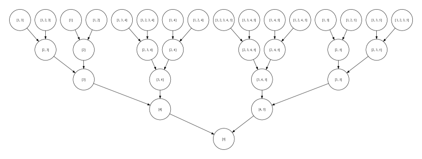
(a) Searchers

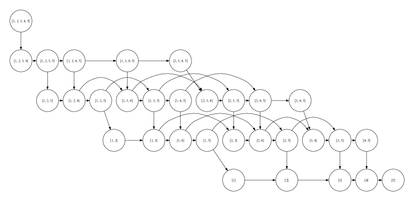
(b) Providers

Figure 15. Transitive reduction of the partially ordered set $\mathcal{W}$ and $m=5$. Nodes correspond to elements in $\mathcal{W}$. A directed edge from $w$ to $w^{\prime}$ if $\mu(\pi,b)>\mu(\pi,b^{\prime})$ (Figure 15(a)) or $\eta(\pi,\mathcal{R},b)>\eta(\pi,\mathcal{R},b^{\prime})$ (Figure 15(b)) based on the properties of top-heavy recall-level metrics (Definition 2.2).

B.1. Worst Case and Total Search Efficiency

Notice that, in our example, there is a single, unique minimal element for both $\mathcal{U}$ and $\mathcal{V}$. In this section, we will prove that this element will always be associated with the lowest-ranked relevant item, $\operatorname{TSE}(\pi,\mathcal{R})$. Throughout these proofs, we will use abbreviations for top-heavy recall-level metric properties defined in Section 2.

Theorem B.1.

If $\mu$ is a top-heavy recall-level metric and $z(1,1)=1$, then

$$\operatorname{WC}_{\mu}(\pi,\mathcal{R}) =\operatorname{TSE}(\pi,\mathcal{R})$$

Proof.

We want to show that, for any $u\in\mathcal{U}$, the performance $\mu(\pi,u)$ is greater than or equal to $\operatorname{TSE}(\pi,\mathcal{R})$, with equality for the user associated with the lowest-ranked relevant item.

Recall that each $w\in\mathcal{W}$ is associated with a $u\in\mathcal{U}$,

$$\mu(\pi,w) \geq e(p_{w_{-1}})z(1,1)$$ top-heaviness

$$=e(p_{w_{-1}}) z(1,1)=1$$

$$\geq e(p_{m}) p_{w_{-1}}\leq p_{m} e(i)>e(i^{\prime}),\forall i<i^{\prime}$$ and

$$=\operatorname{TSE}(\pi,\mathcal{R})$$

∎

Theorem B.2.

If $\eta$ is associated with a top-heavy recall-level metric $\mu$, then

$$\operatorname{WC}_{\eta}(\pi,\mathcal{R}) =\operatorname{TSE}(\pi,\mathcal{R})$$

Proof.

Because all summands of Equation 2 are positive, we know that the minimum $v\in\mathcal{V}$ will correspond to the smallest summand. Moreover, because of the monotonically decreasing exposure, this is the exposure of the lowest ranked relevant item, which is exactly $\operatorname{TSE}(\pi,\mathcal{R})$. ∎

B.2. Leximin and Lexicographic Recall

Let $q_{i}=e(p_{i})$. Since $p$ is sorted in increasing order and $e(x)$ is monotonically decreasing in $x$, $q$ is monotonically decreasing. Assuming we measure the performance of a ranking $\pi$ for a user $u$ as $\mu(\pi,u)$, then we define $\varrho$ to be the $m^{+}\times 1$ vector containing the value of $\mu(\pi,u)$ for each $u\in\mathcal{U}$. We will assume that $\varrho$, like $q$, is sorted in decreasing order.

Lemma B.3.

If $q\succ_{\text{\emph{leximin}}}q^{\prime}$ and $z(1,1)=1$, then the minimum non-tied user is in $\mathcal{W}_{\geq k}-\mathcal{W}_{>k}$, where $k=\min\{i\in[1\mathrel{{.}\,{.}}\nobreak m]|q_{i}\neq q^{\prime}_{i}\}$.

Proof.

Let $k=\min\{i\in[1\mathrel{{.}\,{.}}\nobreak m]|q_{i}\neq q^{\prime}_{i}\}$. Because each $w\in\mathcal{W}_{>k}$ is comprised of indices $i>k$ and because $\forall i>k,p_{i}=p^{\prime}_{i}$, for each associated user $u$, $\mu(p,u)=\mu(p^{\prime},u)$. When computing leximin, by the axiom of the Independence of Identical Consequences (Barbarà and Jackson, 1988), we can remove all of the elements from $\varrho$ and $\varrho^{\prime}$ associated with the $\mathcal{W}_{>k}$. This means that the minimum non-tied pair will be in $\mathcal{W}-\mathcal{W}_{>k}$.

Now we need to show that $\mathcal{W}_{\geq k}-\mathcal{W}_{>k}$ is the set of minimal elements of $\mathcal{W}-\mathcal{W}_{>k}$. This holds if we can show that for every element $w\in\mathcal{W}-\mathcal{W}_{\geq k}$, there exists $w^{\prime}\in\mathcal{W}_{\geq k}-\mathcal{W}_{>k}$, such that $\mu(\pi,w)\geq\mu(\pi,w^{\prime})$.

If $w_{-1}\leq k$ (as depicted by the pink nodes Figure 15), then let $w^{\prime}=\{k\}$,

$$\mu(\pi,w) \geq e(p_{w_{-1}})z(1,1)$$ top-heaviness

$$=e(p_{w_{-1}}) z(1,1)=1$$

$$\geq e(p_{k}) p_{w_{-1}}\leq p_{k} e(i)>e(i^{\prime}),\forall i<i^{\prime}$$ and

$$=\mu(\pi,w^{\prime})$$

If $w_{-1}>k$ and $k\in w$ (as depicted by the blue nodes Figure 15), then we can let $w^{\prime}=\{j\in w:j\geq k\}$.

Let $j=|w|-|w^{\prime}|$,

$$\mu(\pi,w) \geq\sum_{i=j+1}^{|w|}e(p_{w_{i}})z(i-j,|w|-j)$$ top-heaviness

$$=\sum_{i=1}^{|w^{\prime}|}e(p_{w^{\prime}_{i}})z(i,|w^{\prime}|) w^{\prime}$$ definition of

$$=\mu(\pi,w^{\prime})$$

If $w_{-1}>k$ and $k\not\in w$ (as depicted by the green nodes Figure 15), then $w^{\prime}=\{k\}\cup\{j\in w:j>k\}$. Let $j=|w|-|w^{\prime}|$,

$$\mu(\pi,w) \geq\sum_{i=j+1}^{|w|}e(p_{w_{i}})z(i-j,|w|-j)$$ top-heaviness

$$=e(p_{w_{j+1}})z(1,|w|-j)+\sum_{i=j+2}^{|w|}e(p_{w_{i}})z(i-j,|w|-j)$$

$$=e(p_{w_{j+1}})z(1,|w^{\prime}|)+\sum_{i=2}^{|w^{\prime}|}e(p_{w^{\prime}_{i}})z(i,|w^{\prime}|) j w^{\prime}$$ definition of and

$$>e(p_{w^{\prime}_{1}})z(1,|w^{\prime}|)+\sum_{i=2}^{|w^{\prime}|}e(p_{w^{\prime}_{i}})z(i,|w^{\prime}|) p_{w_{j+1}}<p_{k} e(i)>e(i^{\prime}),\forall i<i^{\prime}$$ and

$$=\sum_{i=1}^{|w^{\prime}|}e(p_{w^{\prime}_{i}})z(i,|w^{\prime}|)$$

$$=\mu(\pi,w^{\prime})$$

∎

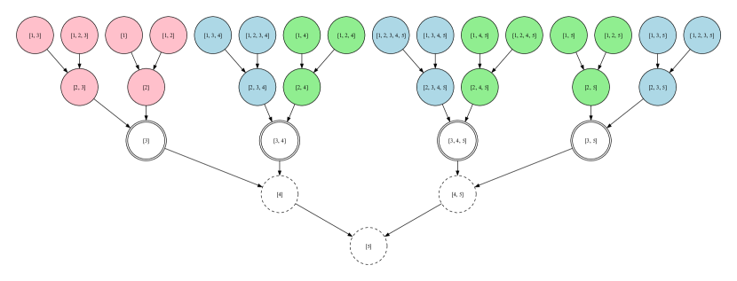
(a) Users. Partitioning $\mathcal{W}$ when $k=3$. $\mathcal{W}$ is partitioned into $\mathcal{W}_{\geq k}-\mathcal{W}_{>k}$ (double circle), $\mathcal{W}_{>k}$ (dashed circle), and $\mathcal{W}-\mathcal{W}_{\geq k}$ (colored circles, described in the proof of Lemma B.3). This figure best rendered in color.

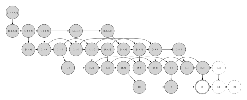
(b) Providers. Assuming $k=3$, then the provider with the minimum exposure is $w=[k]$.

Figure 16. Leximin

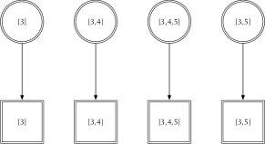
Figure 17. Domination of $\mathcal{W}_{\geq k}-\mathcal{W}_{>k}$. Let $\pi$ be represented by circles and $\pi^{\prime}$ be represented by squares.

Theorem B.4.

$$q\succ_{\text{\emph{leximin}}}q^{\prime}\rightarrow\varrho\succ_{\text{\emph{leximin}}}\varrho^{\prime}$$

Proof.

Case 1 ($q_{m}>q^{\prime}_{m}$).

Theorem B.1 means that $\varrho_{m^{+}}=q_{m}$ and $\varrho^{\prime}_{m^{+}}=q^{\prime}_{m}$ and the implication is true.

Case 2 ($q_{m}=q^{\prime}_{m}$).

Because $q\succ_{\text{leximin}}q^{\prime}$, we know that there exists a $k$ such that $q_{k}>q^{\prime}_{k}$ and $\forall i\in[k+1\mathrel{{.}\,{.}}\nobreak m],q_{i}=q^{\prime}_{i}$ (as depicted in Figure 17). We know from Lemma B.3 that the lowest-ranked, non-tied users are in $\mathcal{W}_{\geq k}-\mathcal{W}_{>k}$.

We want to show that, for every element $w\in\mathcal{W}_{\geq k}-\mathcal{W}_{>k}$, $\pi$ is preferred to $\pi^{\prime}$.

$$\mu(\pi,w) =\sum_{i=1}^{|w|}e(p_{w_{i}})z(i,|w|)$$

$$=e(p_{k})z(1,|w|)+\sum_{i=2}^{|w|}e(p_{w_{i}})z(i,|w|)$$

$$=e(p_{k})z(1,|w|)+\sum_{i=2}^{|w|}e(p^{\prime}_{w_{i}})z(i,|w|) \forall i>k,p_{i}=p^{\prime}_{i}$$

$$>e(p^{\prime}_{k})z(1,|w|)+\sum_{i=2}^{|w|}e(p^{\prime}_{w_{i}})z(i,|w|) p_{k}<p^{\prime}_{k} e(i)>e(i^{\prime}),\forall i<i^{\prime}$$ and

$$=\sum_{i=1}^{|w|}e(p^{\prime}_{w_{i}})z(i,|w|)$$

$$=\mu(\pi^{\prime},w)$$

∎

Theorem B.5.

$$q=_{\text{\emph{leximin}}}q^{\prime}\rightarrow\varrho=_{\text{\emph{leximin}}}\varrho^{\prime}$$

Proof.

The only way that $q=_{\text{leximin}}q^{\prime}$ is when $\forall i\in[1\mathrel{{.}\,{.}}\nobreak m],q_{i}=q^{\prime}_{i}$. If this is the case, then $\forall u\in\mathcal{U},\mu(\pi,u)=\mu(\pi^{\prime},u)$ and, therefore, $\varrho=_{\text{leximin}}\varrho^{\prime}$. ∎

Theorem B.6.

$$q\succ_{\text{\emph{leximin}}}q^{\prime}\rightarrow\phi\succ_{\text{\emph{leximin}}}\phi^{\prime}$$

where, for $v\in\mathcal{V}$, $\phi_{v}=\eta(\pi,\mathcal{R},v)$.

Proof.

Case 1 ($q_{m}>q^{\prime}_{m}$).

We know from the proof of Theorem B.2, the lowest ranked items in $\phi$ and $\phi^{\prime}$ correspond to $e(p_{m})=q_{m}$ and $e(p^{\prime}_{m})=q^{\prime}_{m}$, respectively, and so the proof holds in this case.

Case 2 ($q_{m}=q^{\prime}_{m}$).

Because $q\succ_{\text{leximin}}q^{\prime}$, we know that there exists a $k$ such that $q_{k}>q^{\prime}_{k}$ and $\forall i\in[k+1,m],q_{i}=q^{\prime}_{i}$. The provider $w=[k]$ must be the worst-off non-tied element. Assume that there exists a worse-off non-tied provider. Because $w$ is a singleton and because of monotonically decreasing exposure, this worse off provider must be in $\mathcal{W}_{>k}$. However, we know that these providers are all tied and therefore we have a contradiction.

∎

Appendix C Optimal Rankings

Let $S_{n}^{*}$ be the set of permutations that rank all of the items in $\mathcal{R}$ above $\mathcal{D}-\mathcal{R}$.

Theorem C.1.

Given $\pi^{*}\in S_{n}^{*}$,

$$\min_{u\in\mathcal{U}}\mathbb{E}_{\pi\sim S_{n}^{*}}\left[\mu(\pi,u)\right] \geq\min_{u\in\mathcal{U}}\mu(\pi^{*},u)$$

Proof.

Let $\tilde{u}=\text{argmin}_{u\in\mathcal{U}}\mathbb{E}_{\pi\sim S_{n}^{*}}\left[\mu(\pi,u)\right]$ be the worst-off user for a stochastic ranking and $\check{\pi}=\text{argmin}_{\pi\sim S_{n}^{*}}\mu(\pi,\tilde{u})$ the worst deterministic ranking in $S_{n}^{*}$ for $\tilde{u}$,

$$\mathbb{E}_{\pi\sim S_{n}^{*}}\left[\mu(\pi,\tilde{u})\right] =\frac{1}{C}\sum_{\pi\sim S_{n}^{*}}\mu(\pi,\tilde{u})$$

$$\geq\mu(\check{\pi},\tilde{u})$$

$$\geq\min_{u\in\mathcal{U}}\mu(\check{\pi},u)$$

$$=\min_{u\in\mathcal{U}}\mu(\pi^{*},u)$$

where the final equality follows because $\check{\pi},\pi^{*}\in S_{n}^{*}$ and, therefore, have isometric distributions of user utility. ∎

Appendix D Number of Ties

Theorem D.1.

$$\text{\emph{Pr}}(\pi=_{\text{\emph{LR}}}\pi^{\prime}) =\frac{m!(n-m)!}{n!}$$

Proof.

If we sample a ranking uniformly from $S_{n}$, the probability of any specific $p$ is,

$$\text{Pr}(p) =\frac{C}{|S_{n}|}$$

$$={n\choose m}^{-1}$$

Let $\mathcal{P}_{m}^{n}$ be the set of all size $m$ samples of unique integers from $[1\mathrel{{.}\,{.}}\nobreak n]$.

$$\text{Pr}(\pi=_{\text{LR}}\pi^{\prime}) =\text{Pr}(p=p^{\prime})$$

$$=\sum_{p,p^{\prime}\in\mathcal{P}_{m}^{n}}\text{Pr}(p)\text{Pr}(p^{\prime})\text{I}(p=p^{\prime})$$

$$=\sum_{p\in\mathcal{P}_{m}^{n}}\text{Pr}(p)^{2}$$

$$={n\choose m}\times\frac{1}{{n\choose m}}\times\frac{1}{{n\choose m}}$$

$$=\frac{m!(n-m)!}{n!}$$

∎

Theorem D.2.

$$\text{\emph{Pr}}(\pi=_{\operatorname{TSE}}\pi^{\prime}) ={n\choose m}^{-2}\sum_{i=m}^{n}{i-1\choose m-1}^{2}$$

Proof.

First, we will compute the probability of ranking $\pi$ where the position of the last relevant item is $i$,

$$\text{Pr}(p_{m}=i) =\frac{{i-1\choose m-1}}{{n\choose m}}$$

We can use this to compute the probability of a tie,

$$\text{Pr}(\pi=_{\operatorname{TSE}}\pi^{\prime}) =\text{Pr}(p_{m}=p^{\prime}_{m})$$

$$=\sum_{p,p^{\prime}\in\mathcal{P}_{m}^{n}}\text{Pr}(p)\text{Pr}(p^{\prime})\text{I}(p_{m}=p^{\prime}_{m})$$

$$=\sum_{i=m}^{n}\text{Pr}(p_{m}=i)^{2}$$

$$=\sum_{i=m}^{n}\frac{{i-1\choose m-1}^{2}}{{n\choose m}^{2}}$$

∎

Theorem D.3.

$$\text{\emph{Pr}}(\pi=_{\text{R}_{k}}\pi^{\prime}) ={n\choose m}^{-2}\sum_{i=0}^{m}{{k\choose i}^{2}{n-k\choose m-i}^{2}}$$

Proof.

Let $\text{Rel}(p,k)=\sum_{i=1}^{m}\text{I}(p_{i}\leq k)$. First, we will compute the probability of ranking $\pi$ where $i$ items are ranked above position $k$,

$$\text{Pr}\left(\text{Rel}(p,k)=i\right) =\frac{{k\choose i}{n-k\choose m-i}}{{n\choose m}}$$

We can use this to compute the probability of a tie,

$$\text{Pr}(\pi=_{\text{TSE}}\pi^{\prime}) =\text{Pr}(\text{Rel}(p,k)=\text{Rel}(p^{\prime},k))$$

$$=\sum_{p,p^{\prime}\in\mathcal{P}_{m}^{n}}\text{Pr}(p)\text{Pr}(p^{\prime})\text{I}(\text{Rel}(p,k)=\text{Rel}(p^{\prime},k))$$

$$=\sum_{i=0}^{m}\text{Pr}(\text{Rel}(p,k)=i)^{2}$$

$$=\sum_{i=0}^{m}\frac{{k\choose i}^{2}{n-k\choose m-i}^{2}}{{n\choose m}^{2}}$$

∎

Theorem D.4.

$$\text{\emph{Pr}}(\pi=_{\text{RP}}\pi^{\prime}) ={n\choose m}^{-2}\sum_{i=0}^{m}{{m\choose i}^{2}{n-m\choose m-i}^{2}}$$

Proof.

The proof follows that of Theorem D.3, substituting $m$ for $k$. ∎

References

- (1)
- Amigó et al. (2013) Enrique Amigó, Julio Gonzalo, and Felisa Verdejo. 2013. A General Evaluation Measure for Document Organization Tasks. In Proceedings of the 36th International ACM SIGIR Conference on Research and Development in Information Retrieval (SIGIR ’13). Association for Computing Machinery, New York, NY, USA, 643–652.
- Barbarà and Jackson (1988) Salvador Barbarà and Matthew Jackson. 1988. Maximin, leximin, and the protective criterion: Characterizations and comparisons. Journal of Economic Theory 46, 1 (1988), 34–44. https://doi.org/10.1016/0022-0531(88)90148-2
- Barocas et al. (2019) Solon Barocas, Moritz Hardt, and Arvind Narayanan. 2019. Fairness and Machine Learning: Limitations and Opportunities. fairmlbook.org. http://www.fairmlbook.org.
- Belkin et al. (1982) N. J. Belkin, R. N. Oddy, and H. M. Brooks. 1982. ASK for information retrieval: part I. background and theory. Journal of Documentation 38, 2 (June 1982), 61–71.
- Biega et al. (2019) Asia J. Biega, Fernando Diaz, Michael D. Ekstrand, and Sebastian Kohlmeier. 2019. Overview of the TREC 2019 Fair Ranking Track. In The Twenty-Eighth Text REtrieval Conference (TREC 2019) Proceedings.
- Biega et al. (2018) Asia J. Biega, Krishna P. Gummadi, and Gerhard Weikum. 2018. Equity of Attention: Amortizing Individual Fairness in Rankings. In The 41st International ACM SIGIR Conference on Research & Development in Information Retrieval (SIGIR ’18). ACM, New York, NY, USA, 405–414.
- Bookstein (1979) Abraham Bookstein. 1979. Relevance. Journal of the American Society for Information Science 30, 5 (1979), 269–273. https://doi.org/10.1002/asi.4630300505
- Boyce (1982) Bert Boyce. 1982. Beyond topicality: A two stage view of relevance and the retrieval process. Information Processing & Management 18, 3 (1982), 105–109. https://doi.org/10.1016/0306-4573(82)90033-4
- Boytsov et al. (2013) Leonid Boytsov, Anna Belova, and Peter Westfall. 2013. Deciding on an Adjustment for Multiplicity in IR Experiments. In Proceedings of the 36th International ACM SIGIR Conference on Research and Development in Information Retrieval (SIGIR ’13). Association for Computing Machinery, New York, NY, USA, 403–412. https://doi.org/10.1145/2484028.2484034
- Bruch et al. (2020) Sebastian Bruch, Shuguang Han, Mike Bendersky, and Marc Najork. 2020. A Stochastic Treatment of Learning to Rank Scoring Functions. In Proceedings of the 13th ACM International Conference on Web Search and Data Mining (WSDM 2020).
- Busin and Mizzaro (2013) Luca Busin and Stefano Mizzaro. 2013. Axiometrics: An Axiomatic Approach to Information Retrieval Effectiveness Metrics. In Proceedings of the 2013 Conference on the Theory of Information Retrieval (ICTIR ’13). Association for Computing Machinery, New York, NY, USA, 22–29.
- Cañamares and Castells (2020) Rocío Cañamares and Pablo Castells. 2020. On Target Item Sampling in Offline Recommender System Evaluation. In Proceedings of the 14th ACM Conference on Recommender Systems (RecSys ’20). Association for Computing Machinery, New York, NY, USA, 259–268. https://doi.org/10.1145/3383313.3412259
- Carterette (2011) Ben Carterette. 2011. System effectiveness, user models, and user utility: a conceptual framework for investigation. In Proceedings of the 34th international ACM SIGIR conference on Research and development in Information Retrieval (SIGIR ’11). ACM, New York, NY, USA, 903–912.
- Carterette et al. (2012) Ben Carterette, Evangelos Kanoulas, and Emine Yilmaz. 2012. Incorporating variability in user behavior into systems based evaluation. In Proceedings of the 21st ACM international conference on Information and knowledge management (CIKM ’12). ACM, New York, NY, USA, 135–144.
- Carterette (2012) Benjamin A. Carterette. 2012. Multiple testing in statistical analysis of systems-based information retrieval experiments. ACM Trans. Inf. Syst. 30, 1 (March 2012), 4:1–4:34. https://doi.org/10.1145/2094072.2094076
- Chandar et al. (2020) Praveen Chandar, Fernando Diaz, and Brian St. Thomas. 2020. Beyond Accuracy: Grounding Evaluation Metrics for Human-Machine Learning Systems. https://github.com/pchandar/beyond-accuracy-tutorial. In Advances in Neural Information Processing Systems.
- Clarke et al. (2020) Charles L.A. Clarke, Alexandra Vtyurina, and Mark D. Smucker. 2020. Offline Evaluation without Gain. In Proceedings of the 2020 ACM SIGIR on International Conference on Theory of Information Retrieval (ICTIR ’20). Association for Computing Machinery, New York, NY, USA, 185–192.
- Clarke et al. (2023) Charles L. A. Clarke, Fernando Diaz, and Negar Arabzadeh. 2023. Preference-Based Offline Evaluation. In Proceedings of the Sixteenth ACM International Conference on Web Search and Data Mining (WSDM ’23). Association for Computing Machinery, New York, NY, USA, 1248–1251.
- Clarke et al. (2021) Charles L. A. Clarke, Alexandra Vtyurina, and Mark D. Smucker. 2021. Assessing Top-k Preferences. ACM Trans. Inf. Syst. 39, 3 (may 2021). https://doi.org/10.1145/3451161
- Collins-Thompson et al. (2013) Kevyn Collins-Thompson, Paul Bennett, Fernando Diaz, Charlie Clarke, and Ellen Voorhees. 2013. TREC 2013 Web Track Overview. In The 22nd Text Retrieval Conference Proceedings (TREC 2013). NIST. Special Publication.
- Cooper (2016) Harris M Cooper. 2016. Research synthesis and meta-analysis: a step-by-step approach. SAGE Publications.
- Cooper (1971) W.S. Cooper. 1971. A definition of relevance for information retrieval. Information Storage and Retrieval 7, 1 (1971), 19–37. https://doi.org/10.1016/0020-0271(71)90024-6
- Cooper (1968) William S. Cooper. 1968. Expected search length: A single measure of retrieval effectiveness based on the weak ordering action of retrieval systems. American Documentation 19, 1 (1968), 30–41. https://doi.org/10.1002/asi.5090190108
- Cormack and Grossman (2016) Gordon V. Cormack and Maura R. Grossman. 2016. Engineering Quality and Reliability in Technology-Assisted Review. In Proceedings of the 39th International ACM SIGIR Conference on Research and Development in Information Retrieval (SIGIR ’16). Association for Computing Machinery, New York, NY, USA, 75–84. https://doi.org/10.1145/2911451.2911510
- Cormack and Grossman (2017) Gordon V. Cormack and Maura R. Grossman. 2017. Navigating Imprecision in Relevance Assessments on the Road to Total Recall: Roger and Me. In Proceedings of the 40th International ACM SIGIR Conference on Research and Development in Information Retrieval (SIGIR ’17). Association for Computing Machinery, New York, NY, USA, 5–14.
- Dai et al. (2017) Zhuyun Dai, Yubin Kim, and Jamie Callan. 2017. Learning To Rank Resources. In Proceedings of the 40th International ACM SIGIR Conference on Research and Development in Information Retrieval (SIGIR ’17). Association for Computing Machinery, New York, NY, USA, 837–840.
- d’Aspremont and Gevers (1977) Claude d’Aspremont and Louis Gevers. 1977. Equity and the Informational Basis of Collective Choice. Review of Economic Studies 44, 2 (1977), 199–209.
- Diaz (2015) Fernando Diaz. 2015. Condensed List Relevance Models. In Proceedings of the 2015 International Conference on The Theory of Information Retrieval (ICTIR ’15). ACM, New York, NY, USA, 313–316.
- Diaz and Ferraro (2022) Fernando Diaz and Andres Ferraro. 2022. Offline Retrieval Evaluation Without Evaluation Metrics. In Proceedings of the 45th Annual International ACM SIGIR Conference on Research and Development in Information Retrieval.
- Diaz et al. (2020) Fernando Diaz, Bhaskar Mitra, Michael D. Ekstrand, Asia J. Biega, and Ben Carterette. 2020. Evaluating Stochastic Rankings with Expected Exposure. In Proceedings of the 29th ACM International Conference on Information & Knowledge Management (CIKM ’20). Association for Computing Machinery, New York, NY, USA, 275–284. https://doi.org/10.1145/3340531.3411962
- Do et al. (2021) Virginie Do, Sam Corbett-Davies, Jamal Atif, and Nicolas Usunier. 2021. Two-sided fairness in rankings via Lorenz dominance. In Advances in Neural Information Processing Systems, M. Ranzato, A. Beygelzimer, Y. Dauphin, P.S. Liang, and J. Wortman Vaughan (Eds.), Vol. 34. Curran Associates, Inc., 8596–8608. https://proceedings.neurips.cc/paper/2021/file/48259990138bc03361556fb3f94c5d45-Paper.pdf
- Dou et al. (2007) Zhicheng Dou, Ruihua Song, and Ji-Rong Wen. 2007. A large-scale evaluation and analysis of personalized search strategies. In Proceedings of the 16th international conference on World Wide Web (WWW ’07). ACM, New York, NY, USA, 581–590. https://doi.org/10.1145/1242572.1242651
- Dwork et al. (2001) Cynthia Dwork, Ravi Kumar, Moni Naor, and D. Sivakumar. 2001. Rank Aggregation Methods for the Web. In Proceedings of the 10th International Conference on World Wide Web (WWW ’01). Association for Computing Machinery, New York, NY, USA, 613–622.
- Eikhof and Haunschild (2006) Doris Ruth Eikhof and Axel Haunschild. 2006. Lifestyle Meets Market: Bohemian Entrepreneurs in Creative Industries. Creativity and Innovation Management 15, 3 (2006), 234–241. https://doi.org/10.1111/j.1467-8691.2006.00392.x
- Ekstrand et al. (2022) Michael D. Ekstrand, Anubrata Das, Robin Burke, and Fernando Diaz. 2022. Fairness and Discrimination in Information Access Systems. Foundations and Trends in Information Retrieval.
- Ekstrand et al. (2018) Michael D. Ekstrand, Mucun Tian, Ion Madrazo Azpiazu, Jennifer D. Ekstrand, Oghenemaro Anuyah, David McNeill, and Maria Soledad Pera. 2018. All The Cool Kids, How Do They Fit In?: Popularity and Demographic Biases in Recommender Evaluation and Effectiveness. In Proceedings of the 1st Conference on Fairness, Accountability and Transparency (Proceedings of Machine Learning Research, Vol. 81), Sorelle A. Friedler and Christo Wilson (Eds.). PMLR, New York, NY, USA, 172–186.
- Ferrante et al. (2021) Marco Ferrante, Nicola Ferro, and Norbert Fuhr. 2021. Towards Meaningful Statements in IR Evaluation: Mapping Evaluation Measures to Interval Scales. IEEE Access 9 (2021), 136182–136216.
- Ferrante et al. (2020) Marco Ferrante, Nicola Ferro, and Eleonora Losiouk. 2020. How do interval scales help us with better understanding IR evaluation measures? Information Retrieval Journal 23, 3 (2020), 289–317.
- Ferrante et al. (2015) Marco Ferrante, Nicola Ferro, and Maria Maistro. 2015. Towards a Formal Framework for Utility-Oriented Measurements of Retrieval Effectiveness. In Proceedings of the 2015 International Conference on The Theory of Information Retrieval (ICTIR ’15). Association for Computing Machinery, New York, NY, USA, 21–30.
- Ferrante et al. (2017) Marco Ferrante, Nicola Ferro, and Silvia Pontarollo. 2017. Are IR Evaluation Measures on an Interval Scale?. In Proceedings of the ACM SIGIR International Conference on Theory of Information Retrieval (ICTIR ’17). Association for Computing Machinery, New York, NY, USA, 67–74.
- Ferrante et al. (2019) Marco Ferrante, Nicola Ferro, and Silvia Pontarollo. 2019. A General Theory of IR Evaluation Measures. IEEE Transactions on Knowledge and Data Engineering 31, 3 (2019), 409–422. https://doi.org/10.1109/TKDE.2018.2840708
- Ferraro et al. (2022) Andres Ferraro, Gustavo Ferreira, Fernando Diaz, and Georgina Born. 2022. Measuring Commonality in Recommendation of Cultural Content: Recommender Systems to Enhance Cultural Citizenship. In Proceedings of the 16th ACM Conference on Recommender Systems.
- Flach and Kull (2015) Peter Flach and Meelis Kull. 2015. Precision-Recall-Gain Curves: PR Analysis Done Right. In Advances in Neural Information Processing Systems, C. Cortes, N. Lawrence, D. Lee, M. Sugiyama, and R. Garnett (Eds.), Vol. 28. Curran Associates, Inc.
- Gordon et al. (2021) Mitchell L. Gordon, Kaitlyn Zhou, Kayur Patel, Tatsunori Hashimoto, and Michael S. Bernstein. 2021. The Disagreement Deconvolution: Bringing Machine Learning Performance Metrics In Line With Reality. Association for Computing Machinery, New York, NY, USA. https://doi.org/10.1145/3411764.3445423
- Goren et al. (2018) Gregory Goren, Oren Kurland, Moshe Tennenholtz, and Fiana Raiber. 2018. Ranking Robustness Under Adversarial Document Manipulations. In The 41st International ACM SIGIR Conference on Research & Development in Information Retrieval (SIGIR ’18). Association for Computing Machinery, New York, NY, USA, 395–404. https://doi.org/10.1145/3209978.3210012
- Hadida (2015) Allègre Hadida. 2015. Performance in the Creative Industries. In The Oxford Handbook of Creative Industries. Oxford University Press. https://doi.org/10.1093/oxfordhb/9780199603510.013.018
- Harman (2011) Donna Harman. 2011. Information Retrieval Evaluation. Springer Cham.
- Harter (1992) Stephen P. Harter. 1992. Psychological relevance and information science. Journal of the American Society for Information Science 43, 9 (1992), 602–615.
- Harter (1996) Stephen P. Harter. 1996. Variations in relevance assessments and the measurement of retrieval effectiveness. Journal of the American Society for Information Science 47, 1 (1996), 37–49.
- Hashemi et al. (2020) Helia Hashemi, Mohammad Aliannejadi, Hamed Zamani, and W. Bruce Croft. 2020. ANTIQUE: A Non-factoid Question Answering Benchmark. In Advances in Information Retrieval, Joemon M. Jose, Emine Yilmaz, João Magalhães, Pablo Castells, Nicola Ferro, Mário J. Silva, and Flávio Martins (Eds.). Springer International Publishing, Cham, 166–173.
- Hashimoto et al. (2018) Tatsunori Hashimoto, Megha Srivastava, Hongseok Namkoong, and Percy Liang. 2018. Fairness Without Demographics in Repeated Loss Minimization. In Proceedings of the 35th International Conference on Machine Learning (Proceedings of Machine Learning Research, Vol. 80), Jennifer Dy and Andreas Krause (Eds.). PMLR, Stockholmsmässan, Stockholm Sweden, 1929–1938. http://proceedings.mlr.press/v80/hashimoto18a.html
- Heidari et al. (2019) Hoda Heidari, Michele Loi, Krishna P. Gummadi, and Andreas Krause. 2019. A Moral Framework for Understanding Fair ML through Economic Models of Equality of Opportunity. In Proceedings of the Conference on Fairness, Accountability, and Transparency (FAT* ’19). Association for Computing Machinery, New York, NY, USA, 181–190.
- Herlocker et al. (2004) Jonathan L. Herlocker, Joseph A. Konstan, Loren G. Terveen, and John T. Riedl. 2004. Evaluating Collaborative Filtering Recommender Systems. ACM Trans. Inf. Syst. 22, 1 (jan 2004), 5–53. https://doi.org/10.1145/963770.963772
- Kazai and Lalmas (2006) Gabriella Kazai and Mounia Lalmas. 2006. EXtended Cumulated Gain Measures for the Evaluation of Content-Oriented XML Retrieval. ACM Trans. Inf. Syst. 24, 4 (oct 2006), 503–542.
- Kelly and Teevan (2003) Diane Kelly and Jaime Teevan. 2003. Implicit feedback for inferring user preference: a bibliography. SIGIR Forum 37, 2 (Sept. 2003), 18–28. https://doi.org/10.1145/959258.959260
- Kolm (2002) Serge-Christophe Kolm. 2002. Justice and Equity. MIT Press.
- Leqi et al. (2021) Liu Leqi, Fatma Kilinc-Karzan, Zachary C. Lipton, and Alan L. Montgomery. 2021. Rebounding Bandits for Modeling Satiation Effects.
- Lewis et al. (2021) David D. Lewis, Eugene Yang, and Ophir Frieder. 2021. Certifying One-Phase Technology-Assisted Reviews. Association for Computing Machinery, New York, NY, USA, 893–902. https://doi.org/10.1145/3459637.3482415
- Li et al. (2014) Cheng Li, Yue Wang, Paul Resnick, and Qiaozhu Mei. 2014. ReQ-ReC: High Recall Retrieval with Query Pooling and Interactive Classification. In Proceedings of the 37th International ACM SIGIR Conference on Research & Development in Information Retrieval (SIGIR ’14). Association for Computing Machinery, New York, NY, USA, 163–172.
- Lupu et al. (2017) Mihai Lupu, Katja Mayer, Noriko Kando, and Anthony J. Trippe. 2017. Current Challenges in Patent Information Retrieval. Springer Berlin, Heidelberg.
- Macdonald et al. (2013) Craig Macdonald, Rodrygo L. T. Santos, and Iadh Ounis. 2013. The whens and hows of learning to rank for web search. Information Retrieval 16, 5 (2013), 584–628.
- Mackie et al. (2023) Iain Mackie, Shubham Chatterjee, and Jeffrey Dalton. 2023. Generative and Pseudo-Relevant Feedback for Sparse, Dense and Learned Sparse Retrieval. arXiv:2305.07477 [cs.IR]
- Magdy and Jones (2010a) Walid Magdy and Gareth J.F. Jones. 2010a. PRES: A Score Metric for Evaluating Recall-Oriented Information Retrieval Applications. In Proceedings of the 33rd International ACM SIGIR Conference on Research and Development in Information Retrieval (SIGIR ’10). Association for Computing Machinery, New York, NY, USA, 611–618. https://doi.org/10.1145/1835449.1835551
- Magdy and Jones (2010b) Walid Magdy and Gareth J. F. Jones. 2010b. Examining the Robustness of Evaluation Metrics for Patent Retrieval with Incomplete Relevance Judgements. In Multilingual and Multimodal Information Access Evaluation, Maristella Agosti, Nicola Ferro, Carol Peters, Maarten de Rijke, and Alan Smeaton (Eds.). Springer Berlin Heidelberg, Berlin, Heidelberg, 82–93.
- Mehrotra et al. (2017) Rishabh Mehrotra, Amit Sharma, Ashton Anderson, Fernando Diaz, Hanna Wallach, and Emine Yilmaz. 2017. Auditing Search Engines for Differential Satisfaction Across Demographics. In Proceedings of the 26th International Conference on World Wide Web.
- Memarrast et al. (2021) Omid Memarrast, Ashkan Rezaei, Rizal Fathony, and Brian D. Ziebart. 2021. Fairness for Robust Learning to Rank. CoRR abs/2112.06288 (2021). https://arxiv.org/abs/2112.06288
- Mladenov et al. (2020) Martin Mladenov, Elliot Creager, Omer Ben-Porat, Kevin Swersky, Richard S. Zemel, and Craig Boutilier. 2020. Optimizing Long-term Social Welfare in Recommender Systems: A Constrained Matching Approach. In Proceedings of the 37th International Conference on Machine Learning, ICML 2020, 13-18 July 2020, Virtual Event (Proceedings of Machine Learning Research, Vol. 119). PMLR, 6987–6998. http://proceedings.mlr.press/v119/mladenov20a.html
- Mobasher et al. (2007) Bamshad Mobasher, Robin Burke, Runa Bhaumik, and Chad Williams. 2007. Toward Trustworthy Recommender Systems: An Analysis of Attack Models and Algorithm Robustness. ACM Trans. Internet Technol. 7, 4 (oct 2007), 23–38. https://doi.org/10.1145/1278366.1278372
- Moffat (2013) Alistair Moffat. 2013. Seven Numeric Properties of Effectiveness Metrics. In Information Retrieval Technology, Rafael E. Banchs, Fabrizio Silvestri, Tie-Yan Liu, Min Zhang, Sheng Gao, and Jun Lang (Eds.). Springer Berlin Heidelberg, Berlin, Heidelberg, 1–12.
- Mohammad et al. (2018) Hafeezul Rahman Mohammad, Keyang Xu, Jamie Callan, and J. Shane Culpepper. 2018. Dynamic Shard Cutoff Prediction for Selective Search. In The 41st International ACM SIGIR Conference on Research & Development in Information Retrieval (SIGIR ’18). Association for Computing Machinery, New York, NY, USA, 85–94.
- Montazeralghaem et al. (2020) Ali Montazeralghaem, Hamed Zamani, and James Allan. 2020. A Reinforcement Learning Framework for Relevance Feedback. In Proceedings of the 43rd International ACM SIGIR Conference on Research and Development in Information Retrieval (SIGIR ’20). Association for Computing Machinery, New York, NY, USA, 59–68.
- Moulin (2003) Hervé Moulin. 2003. Fair Division and Collective Welfare. MIT Press.
- National Institute for Standards and Technology (2000) National Institute for Standards and Technology. 2000. Data - English Relevance Judgements. https://trec.nist.gov/data/reljudge_eng.html
- Neophytou et al. (2022) Nicola Neophytou, Bhaskar Mitra, and Catherine Stinson. 2022. Revisiting Popularity and Demographic Biases in Recommender Evaluation and Effectiveness. In Advances in Information Retrieval, Matthias Hagen, Suzan Verberne, Craig Macdonald, Christin Seifert, Krisztian Balog, Kjetil Nørvåg, and Vinay Setty (Eds.). Springer International Publishing, Cham, 641–654.
- Oosterhuis and de Rijke (2020) Harrie Oosterhuis and Maarten de Rijke. 2020. Policy-Aware Unbiased Learning to Rank for Top-k Rankings. In Proceedings of the 43rd International ACM SIGIR Conference on Research and Development in Information Retrieval (SIGIR ’20). Association for Computing Machinery, New York, NY, USA, 489–498.
- Ovaisi et al. (2022) Zohreh Ovaisi, Shelby Heinecke, Jia Li, Yongfeng Zhang, Elena Zheleva, and Caiming Xiong. 2022. RGRecSys: A Toolkit for Robustness Evaluation of Recommender Systems. In Proceedings of the Fifteenth ACM International Conference on Web Search and Data Mining (WSDM ’22). Association for Computing Machinery, New York, NY, USA, 1597–1600.
- Qin et al. (2010) Tao Qin, Tie-Yan Liu, and Hang Li. 2010. A general approximation framework for direct optimization of information retrieval measures. Information Retrieval 13, 4 (2010), 375–397. https://doi.org/10.1007/s10791-009-9124-x
- Radlinski and Joachims (2007) Filip Radlinski and Thorsten Joachims. 2007. Active exploration for learning rankings from clickthrough data. In Proceedings of the 13th ACM SIGKDD International Conference on Knowledge Discovery and Data Mining. Association for Computing Machinery, New York, NY, USA, 570–579.
- Rawls (1974) John Rawls. 1974. Some Reasons for the Maximin Criterion. The American Economic Review 64, 2 (1974), 141–146.
- Rawls (2001) John Rawls. 2001. Justice as Fairness: A Restatement. Harvard University Press.
- Robertson (1977) Stephen Robertson. 1977. The Probability Ranking Principle. Journal of Documentation (1977).
- Robertson (2008) Stephen Robertson. 2008. A New Interpretation of Average Precision. In Proceedings of the 31st Annual International ACM SIGIR Conference on Research and Development in Information Retrieval (SIGIR ’08). Association for Computing Machinery, New York, NY, USA, 689–690.
- Robertson (1969) S. E. Robertson. 1969. The Parametric Description of Retrieval Tests II: Overall Measures. Journal of Documentation 25, 2 (July 1969), 93–107.
- Rocchio (1964) Joseph John Rocchio. 1964. Performance Indices for Document Retrieval Systems. In Information Storage and Retrieval, Gerald Salton (Ed.). Number ISR-8. Harvard University, Chapter III.
- Roegiest et al. (2015) Adam Roegiest, Gordon V. Cormack, Charles L. A. Clarke, and Maura R. Grossman. 2015. TREC 2015 Total Recall Track Overview. In Proceedings of The Twenty-Fourth Text REtrieval Conference, TREC 2015, Gaithersburg, Maryland, USA, November 17-20, 2015 (NIST Special Publication, Vol. 500-319), Ellen M. Voorhees and Angela Ellis (Eds.). National Institute of Standards and Technology (NIST).
- Rudinger et al. (2015) Rachel Rudinger, Pushpendre Rastogi, Francis Ferraro, and Benjamin Van Durme. 2015. Script Induction as Language Modeling. In Proceedings of the 2015 Conference on Empirical Methods in Natural Language Processing. Association for Computational Linguistics, Lisbon, Portugal, 1681–1686.
- Ruthven (2014) Ian Ruthven. 2014. Relevance behaviour in TREC. Journal of Documentation 70, 6 (2022/12/02 2014), 1098–1117. https://doi.org/10.1108/JD-02-2014-0031
- Sajjadi et al. (2018) Mehdi S. M. Sajjadi, Olivier Bachem, Mario Lucic, Olivier Bousquet, and Sylvain Gelly. 2018. Assessing Generative Models via Precision and Recall. In Proceedings of the 32nd International Conference on Neural Information Processing Systems (NIPS’18). Curran Associates Inc., Red Hook, NY, USA, 5234–5243.
- Sakai (2006) Tetsuya Sakai. 2006. A Further Note on Evaluation Metrics for the Task of Finding One Highly Relevant Document. Technical Report 33(2006-DD-054). Toshiba Corporate R&D Center.
- Sakai (2014) Tetsuya Sakai. 2014. Metrics, statistics, tests. In Bridging Between Information Retrieval and Databases - PROMISE Winter School 2013, Revised Tutorial Lectures (Lecture Notes in Computer Science (including subseries Lecture Notes in Artificial Intelligence and Lecture Notes in Bioinformatics)). Springer Verlag, 116–163. https://doi.org/10.1007/978-3-642-54798-0_6 2013 PROMISE Winter School: Bridging Between Information Retrieval and Databases ; Conference date: 04-02-2013 Through 08-02-2013.
- Sakai and Robertson (2008) Tetsuya Sakai and Stephen Robertson. 2008. Modelling A User Population for Designing Information Retrieval Metrics. In Proceedings of The Second International Workshop on Evaluating Information Access (EVIA).
- Sanderson et al. (2010) Mark Sanderson, Monica Lestari Paramita, Paul Clough, and Evangelos Kanoulas. 2010. Do User Preferences and Evaluation Measures Line Up?. In Proceedings of the 33rd International ACM SIGIR Conference on Research and Development in Information Retrieval (SIGIR ’10). Association for Computing Machinery, New York, NY, USA, 555–562.
- Sen (1970) Amartya Sen. 1970. Collective Choice and Social Welfare. Holden-Day.
- Sen (1976) Amartya Sen. 1976. Welfare inequalities and Rawlsian axiomatics. Theory and Decision 7, 4 (1976), 243–262.
- Sen (1977) Amartya Sen. 1977. On Weights and Measures: Informational Constraints in Social Welfare Analysis. Econometrica 45, 7 (1977), 1539–1572.
- Shah et al. (2021) Kulin Shah, Pooja Gupta, Amit Deshpande, and Chiranjib Bhattacharyya. 2021. Rawlsian Fair Adaptation of Deep Learning Classifiers. In Proceedings of the 2021 AAAI/ACM Conference on AI, Ethics, and Society (AIES ’21). Association for Computing Machinery, New York, NY, USA, 936–945.
- Sidgwick (2011) Henry Sidgwick. 2011. The Methods of Ethics. Cambridge University Press.
- Singh and Joachims (2018) Ashudeep Singh and Thorsten Joachims. 2018. Fairness of Exposure in Rankings. In Proceedings of the 24th ACM SIGKDD International Conference on Knowledge Discovery & Data Mining (KDD ’18). ACM, New York, NY, USA, 2219–2228. https://doi.org/10.1145/3219819.3220088
- Smucker et al. (2007) Mark D. Smucker, James Allan, and Ben Carterette. 2007. A Comparison of Statistical Significance Tests for Information Retrieval Evaluation. In Proceedings of the Sixteenth ACM Conference on Conference on Information and Knowledge Management (CIKM ’07). Association for Computing Machinery, New York, NY, USA, 623–632. https://doi.org/10.1145/1321440.1321528
- Sormunen (2002) Eero Sormunen. 2002. Liberal Relevance Criteria of TREC - Counting on Negligible Documents?. In Proceedings of the 25th Annual International ACM SIGIR Conference on Research and Development in Information Retrieval (SIGIR ’02). Association for Computing Machinery, New York, NY, USA, 324–330. https://doi.org/10.1145/564376.564433
- Srinivasan and Sarial-Abi (2021) Raji Srinivasan and Gülen Sarial-Abi. 2021. When Algorithms Fail: Consumers’ Responses to Brand Harm Crises Caused by Algorithm Errors. Journal of Marketing 85, 5 (2021), 74–91.
- Swets (1969) John A. Swets. 1969. Effectiveness of information retrieval methods. American Documentation 20, 1 (1969), 72–89.
- Teevan et al. (2010) Jaime Teevan, Susan T. Dumais, and Eric Horvitz. 2010. Potential for Personalization. ACM Trans. Comput.-Hum. Interact. 17, 1 (April 2010), 4:1–4:31. https://doi.org/10.1145/1721831.1721835
- The Sedona Conference (2009) The Sedona Conference. 2009. Commentary on Achieving Quality in the E-Discovery Process. The Sedona Conference Journal 10 (2009).
- Tomlinson and Hedin (2017) Stephen Tomlinson and Bruce Hedin. 2017. Measuring Effectiveness in the TREC Legal Track. Springer Berlin Heidelberg, Berlin, Heidelberg, 163–182.
- Trippe and Ruthven (2017) Anthony Trippe and Ian Ruthven. 2017. Evaluating Real Patent Retrieval Effectiveness. Springer Berlin Heidelberg, Berlin, Heidelberg, 143–162.
- Valcarce et al. (2020) Daniel Valcarce, Alejandro Bellogín, Javier Parapar, and Pablo Castells. 2020. Assessing ranking metrics in top-N recommendation. Information Retrieval Journal 23, 4 (2020), 411–448.
- Voorhees (2004) E.M. Voorhees. 2004. Overview of the TREC 2004 Robust Track. In Proceedings of the 13th Text REtrieval Conference (TREC 2004).
- Voorhees (1998) Ellen M. Voorhees. 1998. Variations in Relevance Judgments and the Measurement of Retrieval Effectiveness. In Proceedings of the 21st Annual International ACM SIGIR Conference on Research and Development in Information Retrieval (SIGIR ’98). Association for Computing Machinery, New York, NY, USA, 315–323. https://doi.org/10.1145/290941.291017
- Voorhees and Harman (1997) Ellen M. Voorhees and Donna K. Harman. 1997. Overview of the Fifth Text REtrieval Conference (TREC-5). In Proceedings of the Fifth Text REtrieval Conference (TREC-5).
- Vrijenhoek et al. (2022) Sanne Vrijenhoek, Gabriel Bénédict, Mateo Gutierrez Granada, Daan Odijk, and Maarten De Rijke. 2022. RADio – Rank-Aware Divergence Metrics to Measure Normative Diversity in News Recommendations. In Proceedings of the 16th ACM Conference on Recommender Systems (RecSys ’22). Association for Computing Machinery, New York, NY, USA, 208–219.
- Vrijenhoek et al. (2021) Sanne Vrijenhoek, Mesut Kaya, Nadia Metoui, Judith Möller, Daan Odijk, and Natali Helberger. 2021. Recommenders with a Mission: Assessing Diversity in News Recommendations. In Proceedings of the 2021 Conference on Human Information Interaction and Retrieval (CHIIR ’21). Association for Computing Machinery, New York, NY, USA, 173–183.
- Vrijenhoek et al. (2023) Sanne Vrijenhoek, Lien Michiels, Johannes Kruse, Jordi Viader Guerrero, Alain Starke, and Nava Tintarev (Eds.). 2023. Proceedings of the First Workshop on Normative Design and Evaluation of Recommender Systems.
- Wang et al. (2012) Lidan Wang, Paul N. Bennett, and Kevyn Collins-Thompson. 2012. Robust Ranking Models via Risk-Sensitive Optimization. In Proceedings of the 35th International ACM SIGIR Conference on Research and Development in Information Retrieval (SIGIR ’12). Association for Computing Machinery, New York, NY, USA, 761–770. https://doi.org/10.1145/2348283.2348385
- Wen et al. (2022) Hongyi Wen, Xinyang Yi, Tiansheng Yao, Jiaxi Tang, Lichan Hong, and Ed H. Chi. 2022. Distributionally-Robust Recommendations for Improving Worst-Case User Experience. In Proceedings of the ACM Web Conference 2022 (WWW ’22). Association for Computing Machinery, New York, NY, USA, 3606–3610. https://doi.org/10.1145/3485447.3512255
- Xu et al. (2020) Da Xu, Chuanwei Ruan, Evren Korpeoglu, Sushant Kumar, and Kannan Achan. 2020. Adversarial Counterfactual Learning and Evaluation for Recommender System. In Proceedings of the 34th International Conference on Neural Information Processing Systems (NIPS’20). Curran Associates Inc., Red Hook, NY, USA.
- Yager (1997) Ronald R. Yager. 1997. On the analytic representation of the Leximin ordering and its application to flexible constraint propagation. European Journal of Operational Research 102, 1 (1997), 176–192. https://doi.org/10.1016/S0377-2217(96)00217-2
- Zhang et al. (2019) Xueru Zhang, Mohammadmahdi Khaliligarekani, Cem Tekin, and mingyan liu. 2019. Group Retention when Using Machine Learning in Sequential Decision Making: the Interplay between User Dynamics and Fairness. In Advances in Neural Information Processing Systems 32, H. Wallach, H. Larochelle, A. Beygelzimer, F. d'Alché-Buc, E. Fox, and R. Garnett (Eds.). Curran Associates, Inc., 15269–15278. http://papers.nips.cc/paper/9662-group-retention-when-using-machine-learning-in-sequential-decision-making-the-interplay-between-user-dynamics-and-fairness.pdf
- Zhao et al. (2022) Wayne Xin Zhao, Zihan Lin, Zhichao Feng, Pengfei Wang, and Ji-Rong Wen. 2022. A Revisiting Study of Appropriate Offline Evaluation for Top-N Recommendation Algorithms. ACM Trans. Inf. Syst. 41, 2, Article 32 (dec 2022), 41 pages. https://doi.org/10.1145/3545796
- Zheng et al. (2010) Hua Zheng, Dong Wang, Qi Zhang, Hang Li, and Tinghao Yang. 2010. Do Clicks Measure Recommendation Relevancy? An Empirical User Study. In Proceedings of the Fourth ACM Conference on Recommender Systems (RecSys ’10). Association for Computing Machinery, New York, NY, USA, 249–252. https://doi.org/10.1145/1864708.1864759
- Zhu et al. (2021) Ziwei Zhu, Jingu Kim, Trung Nguyen, Aish Fenton, and James Caverlee. 2021. Fairness among New Items in Cold Start Recommender Systems. In Proceedings of the 44th International ACM SIGIR Conference on Research and Development in Information Retrieval (SIGIR ’21). Association for Computing Machinery, New York, NY, USA, 767–776. https://doi.org/10.1145/3404835.3462948
- Zobel et al. (2009) Justin Zobel, Alistair Moffat, and Laurence A.F. Park. 2009. Against Recall: Is It Persistence, Cardinality, Density, Coverage, or Totality? SIGIR Forum 43, 1 (June 2009), 3–8. https://doi.org/10.1145/1670598.1670600
- Zou and Kanoulas (2020) Jie Zou and Evangelos Kanoulas. 2020. Towards Question-Based High-Recall Information Retrieval: Locating the Last Few Relevant Documents for Technology-Assisted Reviews. ACM Trans. Inf. Syst. 38, 3 (may 2020). https://doi.org/10.1145/3388640