A Gradient Boosting Approach for Training Convolutional and Deep Neural Networks

Abstract

Deep learning has revolutionized the computer vision and image classification domains. In this context Convolutional Neural Networks (CNNs) based architectures are the most widely applied models. In this article, we introduced two procedures for training Convolutional Neural Networks (CNNs) and Deep Neural Network based on Gradient Boosting (GB), namely GB-CNN and GB-DNN. These models are trained to fit the gradient of the loss function or pseudo-residuals of previous models. At each iteration, the proposed method adds one dense layer to an exact copy of the previous deep NN model. The weights of the dense layers trained on previous iterations are frozen to prevent over-fitting, permitting the model to fit the new dense as well as to fine-tune the convolutional layers (for GB-CNN) while still utilizing the information already learned. Through extensive experimentation on different 2D-image classification and tabular datasets, the presented models show superior performance in terms of classification accuracy with respect to standard CNN and Deep-NN with the same architectures.

Keywords Convolutional Neural Network  $\cdot$ Deep Neural Network  $\cdot$ Gradient Boosting Machine

The well-known deep learning technique designs a framework using Artificial Neural Network systems (ANNs). The concept of deep learning after introducing the AlexNet [1] model gained even more attention. A high variety of architectures and topologies of deep network models can be constructed by combining different layer types in the model. Likewise, Convolutional Neural Networks (CNNs) have been widely adopted for diverse computer vision tasks, including image classification [2], object detection [3], anomaly detection [4] and segmentation [5]. These models have demonstrated impressive performance. Convolutional models have proven successful in image classification and object recognition, as demonstrated in recent studies such as ResNet [6], Very Deep Convolutional Networks [7], and Understanding Convolutional Networks [8]. These studies show that by increasing the number of convolutional layers, the model becomes more robust in the feature extraction process [7], however, deeper models present numerical difficulties during training [6, 9]. The non-linearity of the network at each layer reduces the gradients and that could lead to a very slow training [9, 10]. One solution for this is to use batch normalization [9] as an intermediate layer for the networks, which helps to stabilize training and reduce the number of training epochs. Another solution is given by Residual neural network (ResNet) [6], which can stack even hundreds of layers skipping the non-linearity by passing information of previous layers directly. It is worthy noting that ResNet also uses batch normalization layers.

In another line of work, the Gradient Boosting Machines (GBMs) decision tree ensembles [11, 12, 13, 14] have become the state of the art for solving tabular classification and regression tasks [15, 16]. GBMs work by training a sequence of regressor models that sequentially learn the information not learnt by previous models. This is done by computing the gradients of the training data with respect to the previous iteration and by fitting the following model to those gradient values or pseudo-residuals. The final model combines all generated models in an additive manner. These ideas have also been applied to sequentially train Neural Networks [17, 18, 19, 20]. In [19], a gradient boosting based approach that uses a weight estimation model to classify image labels is proposed. The model is designed to mimic the ResNet deep neural network architecture and uses boosting functional gradient minimization [12]. In addition, it also involves formulating linear classifiers and feature extraction, where the feature extraction produces input for the linear classifiers, and the resulting approximated values are stacked in a ResNet layer.

In this paper, we propose a novel deep learning training architecture framework based on gradient boosting, which includes two structures: GB-CNN and GB-DNN. GB-CNN, or Gradient Boosted Convolutional Neural Network, is a CNN training architecture based on convolutional layers. On the other hand, GB-DNN is a simpler architecture based only on dense layers more specific for tabular data. Both architectures explicitly use the gradient boosting procedure to build a set of embedded NNs in depth. The approach adds one dense layer at each iteration to a copy of the previous network. Then, the previous dense layers are frozen and the weights of the new added dense layer are trained on the residuals of the previous iteration. In the case of GB-CNN, also the previously trained convolutional layers are fine-tuned at each boosting iteration. The weights of previous layers are frozen to simplify the training of the network and to avoid overfitting to the residuals.

The rest of the paper is organized as follows: In Section II, we review related works in the field. In Section III, we provide an overview of our proposed approach. In Section IV, we describe our experimental setup and present the results of our experiments in Section V, finally, we conclude the paper in the last section.

1 Related Works

Several studies have used the ideas of gradient boosting optimization to build Neural Networks. For instance, in [20] they propose a convex optimization model for training a shallow Neural Network that could reach the global optimum. This is done by adding one hidden neuron at a time to the network, and re-optimizing the whole network by including a $L^{1}$ regularization on the top layer. This top layer serves as a regularizer to effectively remove neurons. However, the model is computationally feasible only for very small number of inputs attributes. In fact, the method is tested experimentally only for 2D datasets. In another line of work, a shallow neural network is sequentially trained as an additive expansion using gradient boosting [21]. The weights of the trained models are stored to form a final neural network. Their idea is to build a single network using a sequential approach avoiding having an ensemble of networks. The work is specific for tabular multi-output regression problems whether the method proposed in this article is a deep architecture valid for both tabular and structured datasets, such as image datasets.

Furthermore, a development of ResNet in the context of boosting theory was proposed in [18]. This model, called BoostResNet, uses residual blocks that are trained during boosting iterations based on [22]. The BoostResNet builds an ensemble of shallow blocks. In a similar proposal, a deep ResNet-like model (ResFGB) is developed in depth by using a linear classifier and gradient-boosting loss minimization [19]. The proposed method is different from these studies in distinct aspects. In contrast to the work presented in [18, 19] the proposed method is based on gradient boosting [11]. Contrary to [19], the underlying architecture of our work can work with any standard deep architecture (with or without convolutional layers) rather than an ad-hoc specific network block. When trained with convolutional layers, the proposed method includes a series of dense layers trained sequentially while jointly fine-tuning previously fitted convolutional layers. In addition, the proposed method reduces the non-linearity complexity by freezing the previously trained dense layers. On the other hand, ResFGB uses a combination of a linear classifiers and a feature extractor, which is updated by stacking a resnet-type layer at each iteration. The [18] study built layer-by-layer a ResNet boosting (BoostResNet) over features. BoostResNet offers a computational advantage over the conventional ResNet due to its reduced complexity, even though the reported performance is not consistently superior.

2 Methodology

In this paper we propose a methodology to train a set of Deep Neural Network models as an additive expansion trained on the residual of a given loss function. The procedure works by adding a new dense layer sequentially to a copy of the previously trained deep regression NN with all dense layers from previous iterations frozen. The motivation behind freezing the trained dense layers is that the model is less likely to adapt to the noise in the data and avoid overfitting. Based on this idea two deep architectures are proposed: one using convolutional layers (GB-CNN) and one with only dense layers (GB-DNN). In the case of GB-CNN, at each iteration, the model learns from the errors made by the previous dense layers also fine-tuning the parameters of the convolutional layers. In GB-DNN architecture, only the newly inserted dense layer is trained at each iteration while simultaneously freezing all previously trained dense layers. In this section, we described the backbone of the proposed methods alongside with its mathematical framework, followed by the used structure for the convolutional layers. In the first subsection, we defined the mathematical framework of the GB-CNN and GB-DNN, followed by the description of the CNN structure used in the GB-CNN method.

2.1 Gradient Boosted Convolutional and Deep Neural Network

For the GB-CNN architecture, we assume the training and test instances with $D={(\mathbf{X}_{i},\mathbf{y}_{i})}_{1}^{N}$ distribution on input $\textbf{X}_{i}\in\mathbb{R}^{B\times{P_{H}}\times{P_{W}}\times{Ch}}$ a 4-dimensional tensor, where the first dimension $\mathbb{R}^{B}$ corresponds to the batch size, the second and third dimensions $\mathbb{R}^{{P_{H}}\times{P_{W}}}$ represent the height and width of each image respectively, and the fourth dimension $\mathbb{R}^{Ch}$ represents the number of color channels. The labels $\mathbf{y}_{i}$ are characterized by a one-hot encoding vector $y_{i}=[y_{i,1},y_{i,2},\dots,y_{i,K}]$, where $K$ is the number of classes, and $y_{i,j}=1$ if the $i^{th}$ data point belongs to class $j$, and $y_{i,j}=0$ otherwise. For the GB-DNN model, we assume the training and test instances with $D={(\mathbf{X}_{i},\mathbf{y}_{i})}_{1}^{N}$ distribution on input $X_{i}\in\mathbb{R}^{F}e$ with $Fe$ features and Response variables with $K$ attributes $y_{i}\in[1,K]$ respectively.

The idea is to learn and update the trainable parameters of the model to accurately estimate the class of unseen data by minimizing the cross-entropy $\ell(\mathbf{y},p)$ loss function

$$\ell(\mathbf{y}_{i},\mathbf{P}_{i})=-\sum_{k=0}^{K}y_{i,k}\log p_{i,k},$$ (1)

where $\mathbf{P}=\{\{p_{i,k}\}_{k=1}^{K}\}_{i=1}^{N}$ is a probability matrix where $p_{i,k}$ is the estimate of the probability for the $i$-th instance of belonging to class $k$. These probabilities are obtained from the raw outputs of the trained regression networks, $F_{k}$, by applying a softmax function to the outputs of the additive model

$$p_{k}(\cdot)=\frac{\exp(F_{k}(\cdot))}{\sum_{l=1}^{K}\exp(F_{l}(\cdot))}.$$ (2)

The final model is built as an additive model of the outputs by combining several networks $S_{t}$ iteratively

$$F_{t}(\mathbf{X}_{i})=F_{t-1}(\mathbf{X}_{i})+\mathbf{\rho_{t}}S_{t}(\mathbf{X}_{i}),$$ (3)

where $\mathbf{\rho_{t}}$ is a vector of weights for each class of the $t-{th}$ additive model $S_{t}(\mathbf{X}_{i})$.

This additive model is built in a step-wise manner. In the GB-CNN, first, a series of layers, including convolution, activation, pooling, batch normalization, dense and flattening layers, is defined as the function $C$

$$C(\mathbf{X}_{i};\mathbf{\Omega})=H(\mathbf{X}_{i}),$$ (4)

where $\mathbf{\Omega}$ is the set of trainable parameters of the model that include weights and biases of all layers, and the function $H(\mathbf{X}_{i})$ represents the output of the network, which is obtained by applying the set of learnable parameters $\mathbf{\Omega}$ to the input $\mathbf{X}_{i}$. While in GB-DNN a first dense layer is initialized with random weights. The model construction is followed by adding a new linear transformation with an activation function, representing the $t$-th dense layer (boosting iteration)

$$S_{t}(\mathbf{M}_{i};\mathbf{W}_{t})=ReLU_{t}(\mathbf{W}_{t}\mathbf{M}_{i}+\mathbf{b}_{i}),$$ (5)

where $\mathbf{W}_{t}$ is the weight matrix and $\mathbf{b}_{t}$ is the bias vector for the $t$-th dense layer respectively, $\mathbf{M}_{i}$ is the feature mapped output from the previous dense layer output for $i$-th instance, and $ReLU(x)=max(0,x)$ is the activation function for the $t$-th dense layer.

Hence, we can define the additive model of the $t$-th boosting iteration to train the parameters for the proposed model

$$S_{t}=S_{t}(S_{t-1} \bigl{(}C(\mathbf{X}_{i};\mathbf{\Omega}_{t}));\mathbf{W}_{t}\bigl{)}.$$ (6)

by minimizing the loss function $\ell$ (Eq.1), using the following objective function,

$$\begin{split}\bigl{(}\rho_{t},S_{t}\bigl{)}=\operatorname*{\arg\!\min}_{(\rho_{t},S_{t})}\sum_{i=1}^{N}\ell(y_{i},F_{t-1}(\mathbf{X}_{i})+\rho_{t}S_{t}).\end{split}$$ (7)

where the trainable parameters of $S_{t-1}$ were trained in the $(t-1)$-th iteration and are now frozen. The optimization process is the same for GB-CNN and GB-DNN although the GB-CNN fine-tunes the convolutional layer at each iteration whether GB-DNN only trains the newly added layer.

The optimization problem (Eq. 7) continues by training the new model on the pseudo-residuals of the previous epoch, $r_{i,t-1}$, which are parallel to the gradient of the loss for step $t-1$

$$r_{i,t-1} =-\left.\frac{\partial\ell(y_{i},F(\mathbf{X}_{i}))}{\partial F(\mathbf{X}_{i})}.\right|_{F(\mathbf{X}_{i})=F_{t-1}(\mathbf{X}_{i})}.$$ (8)

This is done using a regression neural network optimized using the square loss. Since the network is trained using a loss that is different from the desired cross-entropy loss (Eq. 1), we then update the weights of the output layer for each $K$ class label. This is done by computing the $\mathbf{\rho}_{t}$ vector for the $K$ class labels with a line search optimization

$$f(\rho_{t})=\sum_{i=1}^{N}\sum_{k=1}^{K}y_{i,k}ln\left(\frac{exp(F_{t-1,k}(X_{i})+\rho_{t,k}S_{t,k}(X_{i})}{\sum_{j}^{K}exp(F_{t-1,j}(X_{i})+\rho_{t,j}S_{t,j}(X_{i})}\right),$$ (9)

With this line search, a value of $\mathbf{\rho}_{k}$ is obtained for each class. These values are then integrated into the neural network model by multiplying all the weight values from the last layer to the $k$-th output neuron by $\rho_{k}$ for $k=1\dots K$.

In addition, an additional regularization term is included in the proposed models, namely shrinkage rate, which is a constant value $\nu\in(0,1]$ that reduces the contribution of each additive model in the training procedure by $\nu$ in order to prevent overfitting [11]. The schematic description of the proposed GB-CNN method is shown in Algorithm. 1.

Algorithm 1 Training procedure of GB-CNN.

0:  Input image data and related labels $D=\{\mathbf{x}_{i},y_{i}\}_{1}^{N}$

0:  Number of boosting iterations $T$.

0:  Training epoch on mini-batches $E$.

0:  Gradient Boosting loss function $\ell$ (Eq.1).

  Image batch generator $G(D)=\{(\mathbf{x}_{i},y_{i})\}_{1}^{N}$.

  for $e=0$ to $E$ do

     Fit the GB-CNN with one dense layer to images-residual.

     if if the training additive loss converges then

        break

     end if

  end for

  Update the trainable parameters $\mathbf{W}_{0}$.

  Freeze the added dense layer’s parameters $\mathbf{W}_{0}$.

  for $t=1$ to $T-1$ do

     Add a new dense layer.

     for $e=0$ to $E$ do

        Fit the GB-CNN to images-residual.

        if if the training additive loss converges then

           break

        end if

     end for

     Update the trainable parameters $\mathbf{W}_{t}$.

     Freeze the added dense layer’s parameters $\mathbf{W}_{t}$.

     if if the training Gradient Boosting loss converges then

        break

     end if

  end for

  Update the CNNs’ weights.

  return  A fully trained and fine-tuned GB-CNN network.

2.2 Convolutional layers design

Despite the fact that the proposed method could be applied to different CNN architectures, in the following, we describe the design of convolutional and dense layers for the model applied in the experiments.

The applied CNN architecture consists of a sequence of three blocks. Each block has two 2D-convolutional layers, a batch normalization, max pooling and a dropout layer. The dense layers are then connected to the last of these three layers. The configuration of the blocks is the following. The two 2D-convolutional layers in the first block consists of $32\times 3\times 3$ filters and ReLU as the activation function. The subsequent block has two more 2D-convolutional layers with 64 filters. The convolutional layers of the final block are of size 128. The concatenated layers are two 2D-convolutional layers with 128 filters. All 2D-convolutional layers use filters of size (3x3). After the second convolutional layer of each block, batch normalization is applied to stabilize the distribution of activations. Then a max pooling layer of size (2, 2) is applied to the output to reduce the spatial dependence of the feature maps and increase the invariance to small translations, and finally a dropout layer is included to prevent overfitting with 0.2, 0.3 and 0.4 for each block respectively. Finally, the output is flatten and connected to fully connected dense layers. The dense layers are added and trained iteratively while freezing previous dense layers. This model is compared to the same architecture trained jointly as a standard CNN model. The second proposed architecture considers only the iterative training of a network composed only of dense layers.

This process is illustrated in Fig. 1 in which only the dense layers are shown (Note, that the figure is not representing the actual size of the used dense layers). In the first, iteration, one single dense (and output) layer is trained (dark grey units in left diagram of Fig. 1). This layer is the first fully connected layer. After fitting this model, the model is copied and a second dense layer is added (iteration 1 and second diagram in Fig. 1) freezing the weights of the first dense layer froze (shown in the Fig. 1 with light gray neurons). This second step fine-tunes the parameters of the convolutional layers (if present), skips the training of the previous dense layer, and trains the newly added dense layer (dark gray units). Each new model, fits the last dense layers and the convolutional blocks to the corresponding pseudo-residuals. The training procedure continues until convergence.

We carried out several preliminary analysis in which we compared the performance of the presented method with respect to the same procedure but without applying the freezing of previous layers. These experiments showed that freezing improved the performance. This could be explained as new models are trained on smaller residuals and including more complex models (i.e. unfrozen) could lead to overfitting.

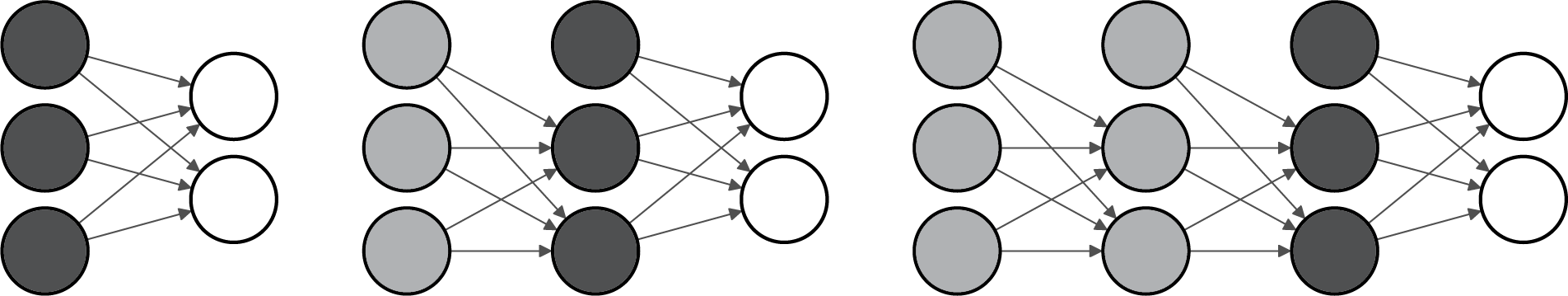
Figure 1: A snippet of the iterative model training procedure. Light-gray indicates that the layer is frozen, dark gray that the layer is being trained and white indicates output layer (also being trained)

3 Experiments

In order to evaluate the proposed new methods structure for Convolutional (GB-CNN) and Deep Neural Networks (GB-DNN), several supervised 2D-image classification tasks and tabular datasets were considered. In the image datasets, the proposed model (GB-CNN) is compared with respect to a CNN model that uses the same architecture and configuration, although with more dense layers (more details below). In the tabular datasets, GB-DNN is compared with a deep neural network with same settings and layers. The objective of our experiments was to evaluate the performance of the tested methods in terms of accuracy and to determine its usefulness for solving the 2D-image and tabular classification problems. The code of the proposed models is made available on github as GB-CNN.

Table 1: Dataset Properties for Image Classification Tasks

Name	train/test	$P_{H}\times P_{W}$	$K$	$Ch$
MNIST [23]	60,000/10,000	$28\times 28$	10	$1$
CIFAR-10 [24]	50,000/10,000	$32\times 32$	10	$3$
Rice varieties [25]	56,250/18,750	$32\times 32$	5	$3$
Fashion-MNIST [26]	60,000/10,000	$28\times 28$	10	$1$
Kuzushiji-MNIST [27]	60,000/10,000	$28\times 28$	10	$1$
MNIST-Corrupted [27]	60,000/10,000	$28\times 28$	10	$1$
Rock-Paper-Scissors [28]	2,520/370	$32\times 32$	3	3

Regarding the 2D-image classification problem, seven 2D-image datasets of various areas of application, class labels, instances, pixel resolution, and color channels are used in this study, as described in Table 1 for the convolutional models. In this experiment, a data generator was used to generate batches of training data on-the-fly during the training process. This allowed us to train the model on a large dataset, without having to load the entire dataset into GPU memory. Moreover, the generator shuffled the data, applied data augmentation techniques (including rescaling the pixel values), and yielded batches with a size of 128. The common hyperparameters and settings of the used GB-CNN and CNN were the same, including the structure of the convolutional layers (described before), the number of hidden neurons in each dense (set to 20), a learning rate of 0.001, and 200 epochs for training with early stopping to prevent overfitting. The shrinkage rate of GB-CNN, used to combine the different generated CNNs, was set to 0.1. As previously described, the proposed method adds one dense layer at each iteration to a copy of the model of the previous iteration. The maximum number of dense layers/iterations was set to 10. Although, GB-CNN generally converges after 2 or 3 iterations. This will be shown in the first experiment in which we analyze the evolution of the loss and accuracy for the tested models. The number of dense layers for CNN was left at 10. Furthermore, we conducted an additional experiment wherein three images (MNIST, Fashion-MNIST, and CIFAR-10) were analyzed using two dense layers, each with a size of 128 and identical settings, in order to investigate the impact of the size of the dense layers in the experimental outcomes.

Table 2: Dataset Properties for Image Classification Tasks

Name	instances	Features	class labels
Digits [29]	1797	64	10
Ionosphere [29]	351	34	2
Letter-26 [29]	20,000	16	26
Sonar	208	2	60
USPS [30]	9,298	256	10
Vowel [29]	990	10	11
Waveform [29]	5,000	21	3

Moreover, in this work, tabular classification datasets from different sources [29, 30] were also tested. The characteristics of these datasets are shown in Table 2. The classifications tasks are of different types, ranging from radar data to handwritten digits and vowel pronunciation. The hyperparameter values of the proposed GB-DNN and the standard Deep-NN are identical. For these datasets, the training was performed using 10-fold cross-validation. In order to determine the optimal values for hyper-parameter of the models, a with-in train grid search process was applied. The test values for the hyper-parameters are: learning rate of both models (ranging from 0.1 to 0.001) and shrinkage rate $\nu$ (ranging from 0.1 to 1.0) of the GB-DNN model. Both models are composed of three dense layers, each with a size of 100 neurons and ReLU as the activation function.

4 Results

In order to analyze the convergence rate of the proposed method, a first batch of experiments was carried out that registered the loss and accuracy of the method after each iteration. We further monitored the loss function across various additive models during training for GB-CNN. The experiment was conducted using the CIFAR-10 dataset, and the evolution of the loss and accuracy was measured in both training and test data points. Also the standard CNN was monitored in the same way. Both models were configured with the same hyperparameters, including identical convolutional layers as outlined in Section III subsection B, and 10 dense layers with a size of 20. The learning rate was set to $0.001$, with a batch size of $128$, and $100$ training epochs for both models. In the case of GB-CNN, the shrinkage was set to $0.01$. The results are shown in Figures 2–5, and Figures 6 and 7).

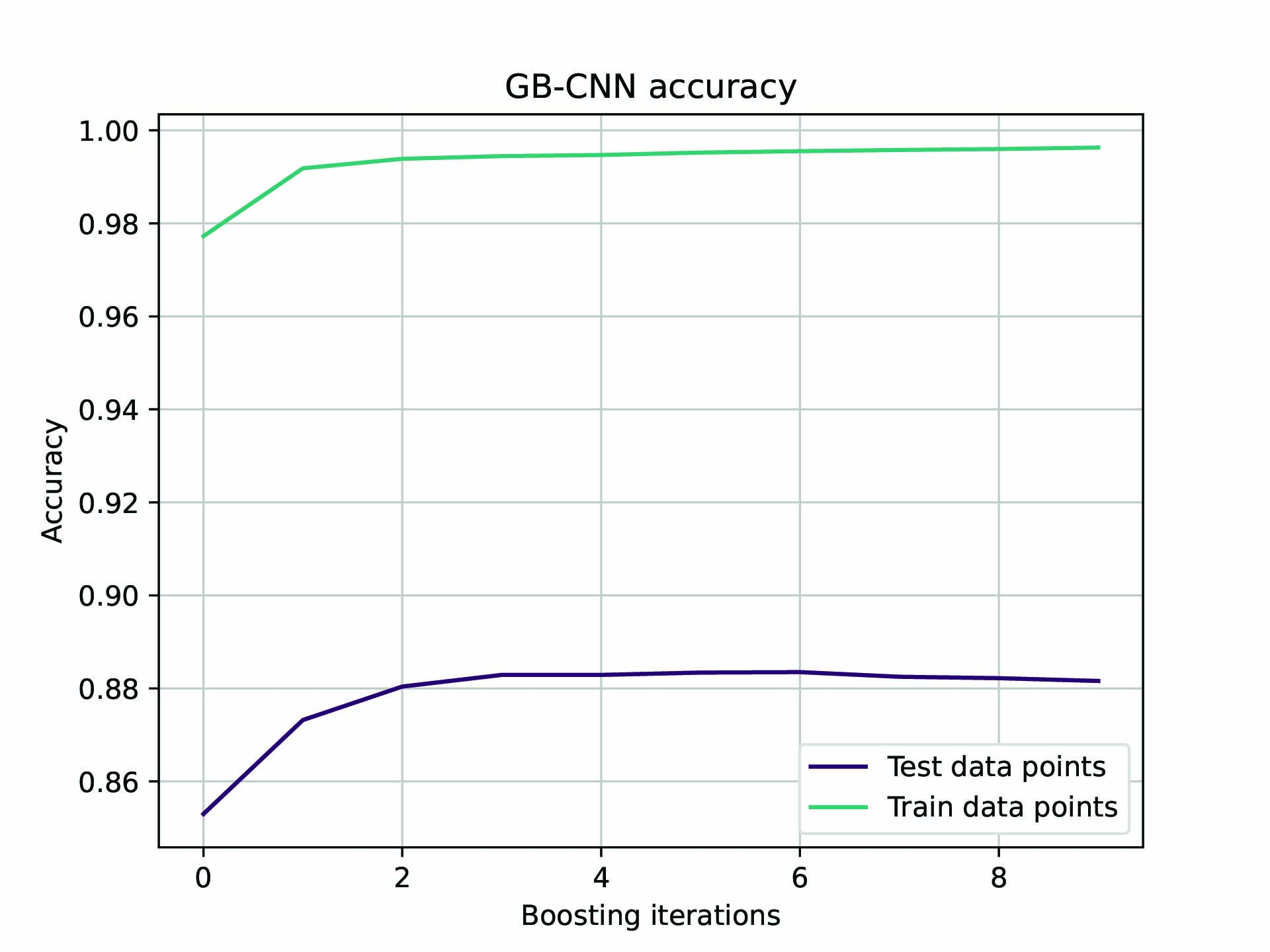
Figure 2: GB-CNN train and test accuracy on CIFAR10 with respect to the number of boosting iterations

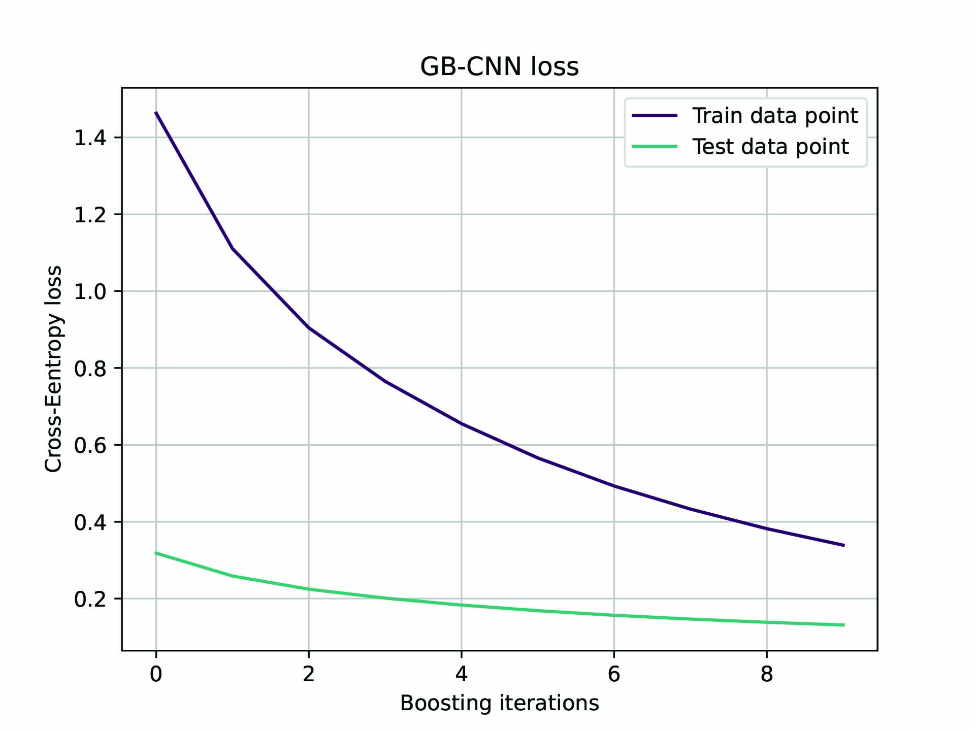
Figure 3: GB-CNN train and test cross-entropy loss on CIFAR10 with respect to the number of boosting iterations

The evolution performance for GB-CNN is shown in Figs. 2–5. Fig. 2 illustrates the train and test accuracy of the model with respect to the number of boosting iterations. In Fig. 3, the average cross-entropy loss across various boosting iterations is shown. Additionally, Figs. 4 and 5 provide an overview of the evolution of the mean square error (MSE) of the additive models created during the boosting iterations with respect to the number of epochs. Note that the loss here is measured as MSE since the individual models trained during boosting are regression networks. From plots in Figs. 2 and 3, it can be observed that the proposed model converges after few booting iterations. Specifically, after three boosting iterations the model has converged and the training process could be stopped. A similar tendency can be observed from the learning evolution of the individual trained networks shown in Figs. 4 for train and 5 for test. We can observe that the first models reduce the loss more significantly. Again, after a few iterations the benefit of adding more models is reduced. Based on these results, for the next experiments we will limit the number of boosting iterations to 2-3.

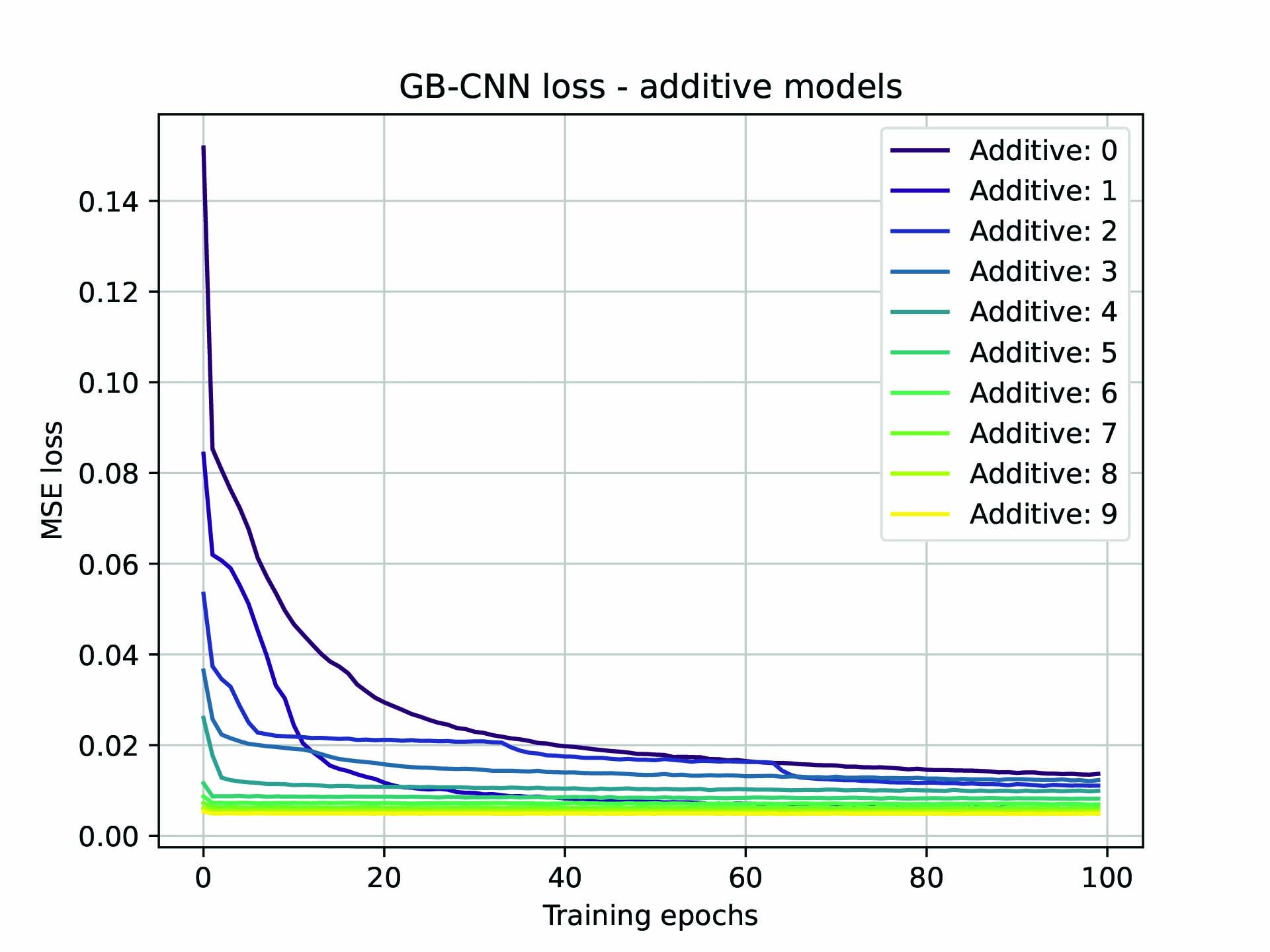
Figure 4: GB-CNN - Additive model train MSE loss on CIFAR10 with respect to the number of boosting iterations

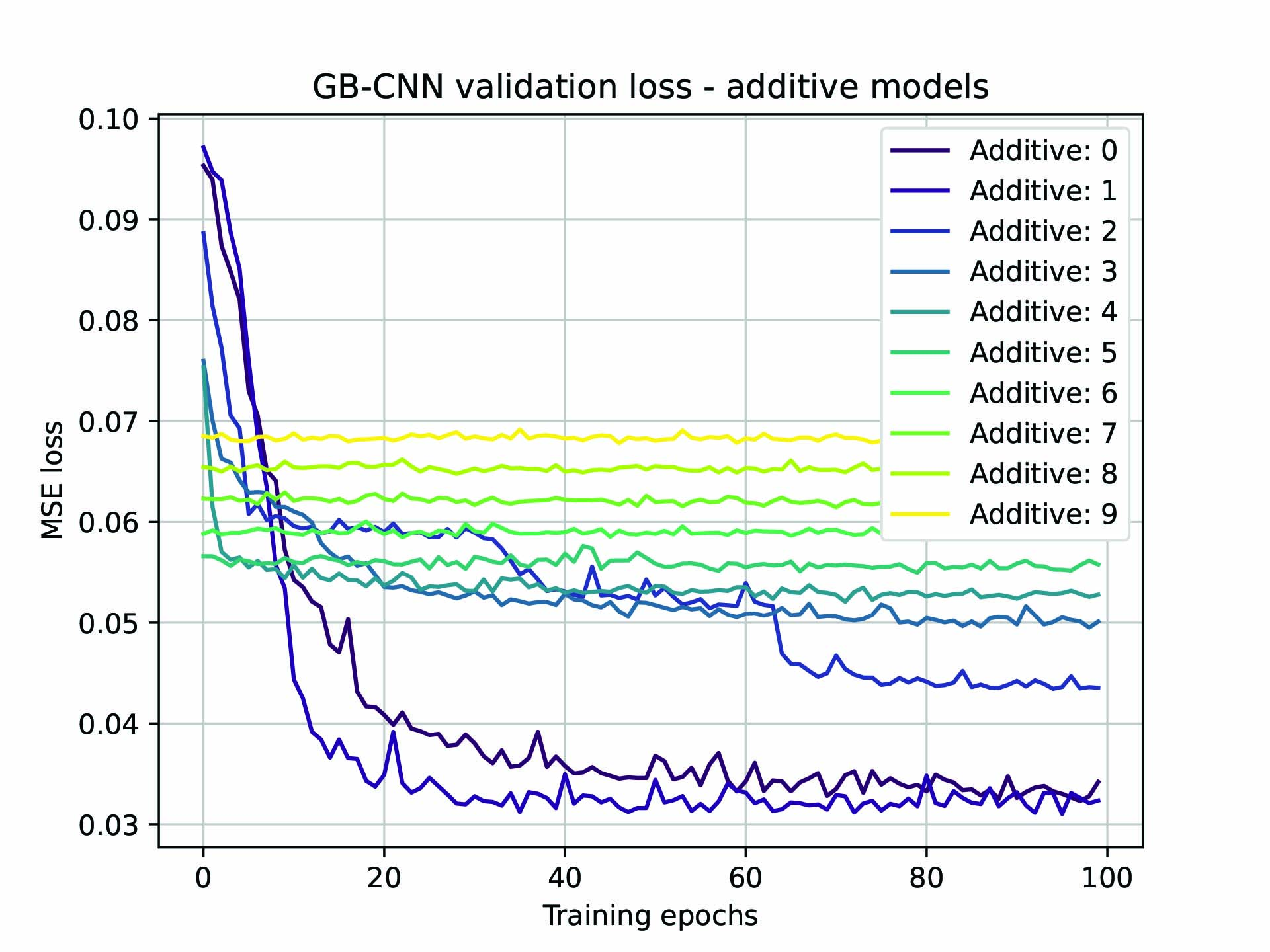
Figure 5: GB-CNN - Additive model test MSE loss on CIFAR10 with respect to the number of boosting iterations

On the other hand, Figs. 6 and 7 present the performance of the CNN model with respect to the training epochs. Specifically, the train and test accuracy and cross-entropy loss of the model are depicted in Figs. 6 and Figs. 7, respectively. As it can be observed from these plots, the CNN model has converged in terms of test accuracy and loss after 100 epochs. This final performance is slightly better to the one achieved by GB-CNN after the first iteration (see Figs. 2 and 3). This makes sense since the first boosting iteration is also a CNN model, although simpler since it has only one dense layer. The most interesting point is that when more layers are included (and models), the proposed GB-CNN architecture manages to further learn at the point where the CNN has converged. In this way, the final performance of the proposed method is better than that of the CNN. In the following a more comprehensive comparison is carried out including the described datasets.

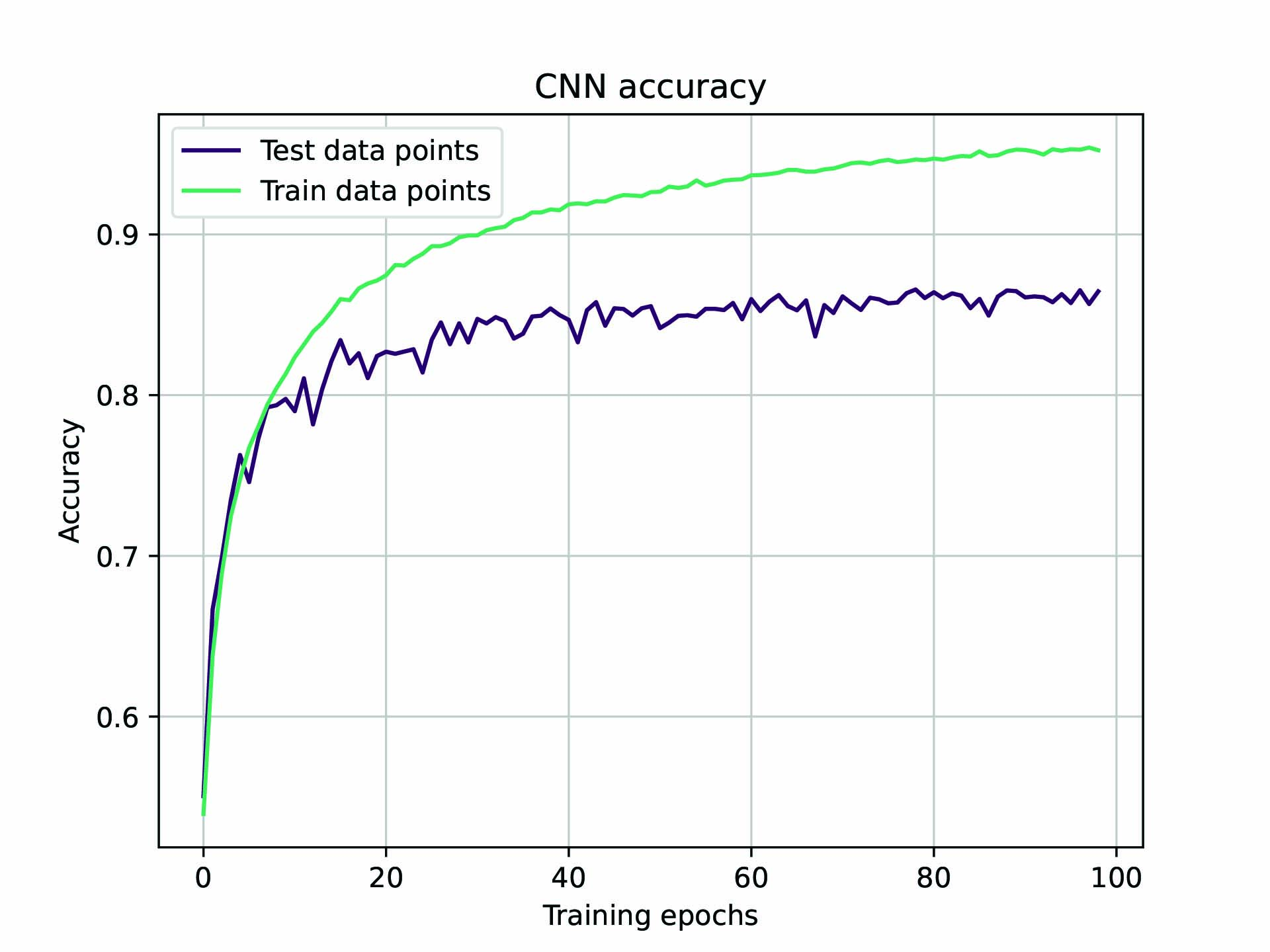
Figure 6: CNN train and test accuracy on CIFAR10 with respect to the training epochs

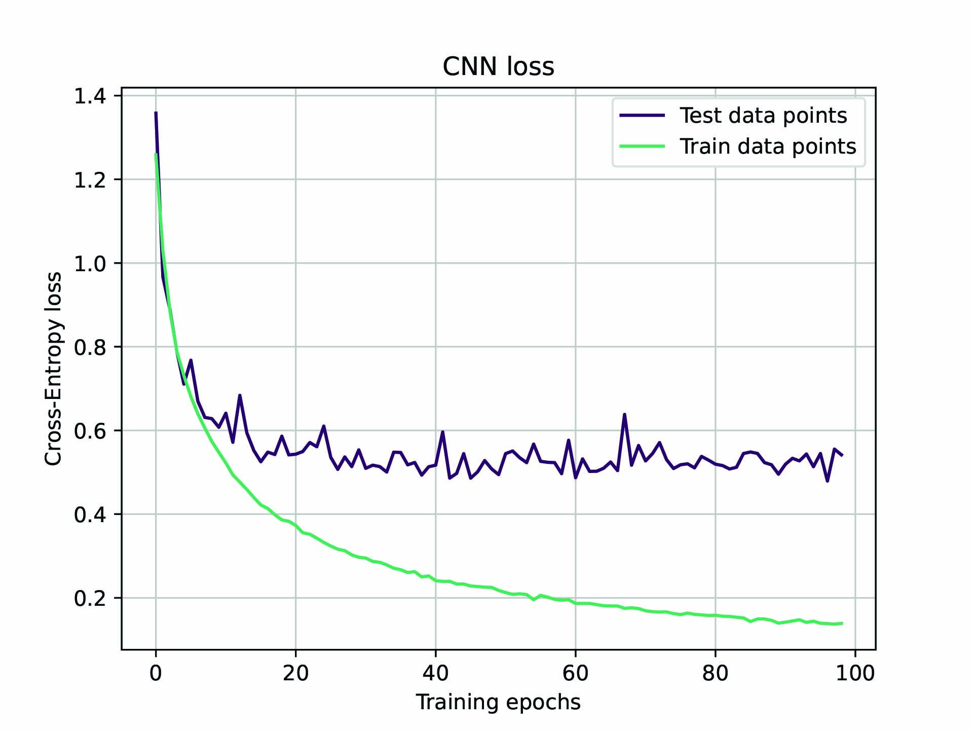
Figure 7: CNN train and test cross-entropy loss on CIFAR10 with respect to the training epochs

Tables 3, 4 and 5 show the generalization accuracy results estimated in the test subsets for the analyzed datasets and models. Table 3 show the results for the convolutional models (GB-CNN and CNN) using 20 neuron in the dense hidden layers. Table 4 include the results for selected image datasets and with larger dense layers of 128 neurons. Finally, Table 5 portray the results for the deep models (GB-DNN and DNN) in the tabular datasets. The best results of the tables are highlighted using a gray background.

As it can be observed in Table 3, the generalization accuracy of the proposed convolutional model (GB-CNN) is higher than that of the baseline CNN model across all tested datasets. The difference is specially large on the Rock-Paper-Scissors. The proposed model achieved an accuracy of $87.37\%$, which is $19.36\%$ higher than the accuracy of CNN ($68.01\%$). On the other datasets the differences are small but consistently in favor of the proposed architecture. For instance, in CIFAR-10, the proposed model achieved an accuracy of $87.65\%$ with respect to the $86.71\%$ that achieves the CNN. In the MNIST dataset, well-known for its simplicity and high accuracy that the CNN models obtain, GB-CNN was able to achieve a remarkable accuracy of $99.61\%$, which is higher than the accuracy of CNN by a very small margin ($0.06$).

Table 3: Accuracy of GB-CNN and CNN models on the experiment with a 20-neuron dense layer. The best results are highlighted in gray

2D-Image dataset	GB-CNN	CNN
MNIST	$99.61\%$	$99.55\%$
CIFAR-10	$87.65\%$	$86.71\%$
Rice varieties	$99.82\%$	$98.37\%$
Fashion-MNIST	$94.34\%$	$93.61\%$
Kuzushiji-MNIST	$98.40\%$	$96.70\%$
MNIST-Corrupted	$99.58\%$	$99.35\%$
Rock-Paper-Scissors	$87.37\%$	$68.01\%$

In relation to the experiment involving the utilization of a dense layer with a larger size (128), the accuracy results for the GB-CNN and CNN models are presented in Table 4. These models were trained and evaluated on three distinct datasets: MNIST, CIFAR-10, and Fashion-MNIST. The findings demonstrate that the GB-CNN model outperformed the CNN model across all these three datasets. Nonetheless, closer examination of the table reveals that the results obtained using 128 dense layers (as shown in Table 4) are slightly inferior to those using 20 neuron layers (as shown in Table 3). This implies that for these particular datasets, employing a greater number of smaller layers may be more effective for capturing the information of the tasks.

Table 4: Accuracy of GB-CNN and CNN models on the experiment with a 128-neuron dense layer. The best results are highlighted in gray

2D-Image dataset	GB-CNN	CNN
MNIST	$99.66\%$	$99.40\%$
CIFAR-10	$86.72\%$	$86.30\%$
Fashion-MNIST	$94.02\%$	$92.38\%$

The results for the tabular datasets summarized in Table 5 for GB-DNN and Deep-NN. The results demonstrate that GB-DNN outperforms Deep-NN in most of the datasets. In particular, GB-DNN achieved the highest accuracy in the Digits, Ionosphere, Letter-26, USPS, Vowel, and Waveform datasets. Deep-NN, on the other hand, achieved the highest accuracy in the Sonar dataset. As in previous results, the differences are in general small with higher difference in Waveform in favor of GB-CNN ($2.82$-point difference) and in Sonar in favor of Deep-NN ($1.45$-point difference). Finally, comparing the results of the proposed method with respect to the work of [19], it can be observed that in the three common tasks our method outperforms ResFGB in two tasks (MNIST and USPS) and is outperformed in one (Letter-26) with the advantage of our method of being much simpler and composed of standard network layers.

Table 5: Accuracy of GB-DNN and Deep-NN models. The best results are highlighted in gray

Tabular dataset	GB-DNN	Deep-NN
Digits	$98.22\%$ $\pm$1.24	$97.55\%$ $\pm$1.06
Ionosphere	$94.87\%$ $\pm$3.08	$94.60\%$ $\pm$3.66
Letter-26	$95.50\%$ $\pm$0.49	$95.29\%$ $\pm$0.63
Sonar	$86.55\%$ $\pm$9.03	$88.00\%$ $\pm$3.78
USPS	$97.39\%$ $\pm$0.40	$96.95\%$ $\pm$0.62
Vowel	$98.08\%$ $\pm$1.59	$97.47\%$ $\pm$2.08
Waveform	$85.20\%$ $\pm$1.89	$82.38\%$ $\pm$2.37

5 Conclusion

This paper presents a novel training approach for training a set of deep neural networks based on convolutional (CNNs) and deep (DNNs) architectures, called GB-CNN and GB-DNN respectively. The proposed training procedures are based on gradient boosting algorithm, which trains iteratively a set of models in order to learn the information not captured in previous iterations. Additionally, both proposed models employ an inner dense layer freezing approach to reduce model complexity and non-linearity.

To evaluate the effectiveness of the proposed models, we conducted experiments on various 2D-images and tabular datasets, ranging from radar data to handwritten digits, fashion, and agriculture areas. Our results demonstrate that the proposed GB-CNN model outperforms traditional CNN models using the same architecture in terms of accuracy in all the analyzed image datasets. Moreover, the GB-DNN model outperforms DNN models in terms of accuracy on most of the studied tabular datasets.

An analysis of the convergence of the proposed model showed that it converges after few boosting iterations. More interestingly, during these iterations the proposed methodology is able to improve the performance of the previous models after the point in which a standard single CNN has converged. This shows that the proposed GB-CNN and GB-DNN models represent a robust and effective solution for 2D-image and tabular classification tasks. Further research and analysis of these models need to be carried out for practical applications in the future.

References

- [1] Alex Krizhevsky, Ilya Sutskever, and Geoffrey E. Hinton. Imagenet classification with deep convolutional neural networks. In F. Pereira, C. J. C. Burges, L. Bottou, and K. Q. Weinberger, editors, Advances in Neural Information Processing Systems 25, pages 1097–1105. Curran Associates, Inc., 2012.
- [2] Dongmei Han, Qigang Liu, and Weiguo Fan. A new image classification method using cnn transfer learning and web data augmentation. Expert Systems with Applications, 95:43–56, 2018.
- [3] Shaoqing Ren, Kaiming He, Ross Girshick, and Jian Sun. Faster r-cnn: Towards real-time object detection with region proposal networks. Advances in neural information processing systems, 28, 2015.
- [4] Taejoon Kim, Sang C Suh, Hyunjoo Kim, Jonghyun Kim, and Jinoh Kim. An encoding technique for cnn-based network anomaly detection. In 2018 IEEE International Conference on Big Data (Big Data), pages 2960–2965. IEEE, 2018.
- [5] Konstantinos Kamnitsas, Christian Ledig, Virginia FJ Newcombe, Joanna P Simpson, Andrew D Kane, David K Menon, Daniel Rueckert, and Ben Glocker. Efficient multi-scale 3d cnn with fully connected crf for accurate brain lesion segmentation. Medical image analysis, 36:61–78, 2017.
- [6] Kaiming He, Xiangyu Zhang, Shaoqing Ren, and Jian Sun. Deep residual learning for image recognition. In Proceedings of the IEEE conference on computer vision and pattern recognition, pages 770–778, 2016.
- [7] Karen Simonyan and Andrew Zisserman. Very deep convolutional networks for large-scale image recognition. arXiv preprint arXiv:1409.1556, 2014.
- [8] Matthew D Zeiler and Rob Fergus. Visualizing and understanding convolutional networks. In European conference on computer vision, pages 818–833. Springer, 2014.
- [9] Sergey Ioffe and Christian Szegedy. Batch normalization: Accelerating deep network training by reducing internal covariate shift. In International conference on machine learning, pages 448–456. PMLR, 2015.
- [10] Xavier Glorot and Yoshua Bengio. Understanding the difficulty of training deep feedforward neural networks. In Proceedings of the thirteenth international conference on artificial intelligence and statistics, pages 249–256. JMLR Workshop and Conference Proceedings, 2010.
- [11] Jerome H Friedman. Greedy function approximation: a gradient boosting machine. Annals of statistics, pages 1189–1232, 2001.
- [12] Llew Mason, Jonathan Baxter, Peter Bartlett, and Marcus Frean. Boosting algorithms as gradient descent. Advances in neural information processing systems, 12, 1999.
- [13] Guolin Ke, Qi Meng, Thomas Finley, Taifeng Wang, Wei Chen, Weidong Ma, Qiwei Ye, and Tie-Yan Liu. Lightgbm: A highly efficient gradient boosting decision tree. Advances in neural information processing systems, 30, 2017.
- [14] Tianqi Chen, Tong He, Michael Benesty, Vadim Khotilovich, Yuan Tang, Hyunsu Cho, Kailong Chen, et al. Xgboost: extreme gradient boosting. R package version 0.4-2, 1(4):1–4, 2015.
- [15] Ravid Shwartz-Ziv and Amitai Armon. Tabular data: Deep learning is not all you need. Information Fusion, 81:84–90, 2022.
- [16] Candice Bentéjac, Anna Csörgő, and Gonzalo Martínez-Muñoz. A comparative analysis of gradient boosting algorithms. Artificial Intelligence Review, 54:1937–1967, 2021.
- [17] Seyedsaman Emami and Gonzalo Martínez-Muñoz. Multioutput regression neural network training via gradient boosting. pages 145–150, 01 2022.
- [18] Furong Huang, Jordan Ash, John Langford, and Robert Schapire. Learning deep resnet blocks sequentially using boosting theory. In International Conference on Machine Learning, pages 2058–2067. PMLR, 2018.
- [19] Atsushi Nitanda and Taiji Suzuki. Functional gradient boosting based on residual network perception. In International Conference on Machine Learning, pages 3819–3828. PMLR, 2018.
- [20] Yoshua Bengio, Nicolas Roux, Pascal Vincent, Olivier Delalleau, and Patrice Marcotte. Convex neural networks. Advances in neural information processing systems, 18, 2005.
- [21] Seyedsaman Emami and Gonzalo Martínez-Muñoz. Sequential training of neural networks with gradient boosting. arXiv preprint arXiv:1909.12098, 2019.
- [22] Yoav Freund and Robert E Schapire. A decision-theoretic generalization of on-line learning and an application to boosting. Journal of computer and system sciences, 55(1):119–139, 1997.
- [23] Norman Mu and Justin Gilmer. Mnist-c: A robustness benchmark for computer vision. arXiv preprint arXiv:1906.02337, 2019.
- [24] Alex Krizhevsky. Learning multiple layers of features from tiny images. Technical report, 2009.
- [25] Murat Koklu, Ilkay Cinar, and Yavuz Selim Taspinar. Classification of rice varieties with deep learning methods. Computers and electronics in agriculture, 187:106285, 2021.
- [26] Han Xiao, Kashif Rasul, and Roland Vollgraf. Fashion-mnist: a novel image dataset for benchmarking machine learning algorithms. arXiv preprint arXiv:1708.07747, 2017.
- [27] Tarin Clanuwat, Mikel Bober-Irizar, Asanobu Kitamoto, Alex Lamb, Kazuaki Yamamoto, and David Ha. Deep learning for classical japanese literature. arXiv preprint arXiv:1812.01718, 2018.
- [28] Laurence Moroney. Rock, paper, scissors dataset, feb 2019.
- [29] M. Lichman. UCI machine learning repository, 2013.
- [30] Jonathan J. Hull. A database for handwritten text recognition research. IEEE Transactions on pattern analysis and machine intelligence, 16(5):550–554, 1994.