The AGNIFS survey: spatially resolved observations of hot molecular and ionised outflows in nearby active galaxies

Abstract

We present the hot molecular and warm ionised gas kinematics for 33 nearby ($0.001\lesssim z\lesssim 0.056$) X-ray selected active galaxies using the H${}_{2}\,2.1218\,\mu$m and Br$\gamma$ emission lines observed in the K-band with the Gemini Near-Infrared Field Spectrograph (NIFS). The observations cover the inner 0.04–2 kpc of each AGN at spatial resolutions of 4-250 pc with a velocity resolution of $\sigma_{\rm inst}\approx$20 ${\rm km\,s^{-1}}$. We find that 31 objects (94 per cent) present a kinematically disturbed region (KDR) seen in ionised gas, while such regions are observed in hot molecular gas for 25 galaxies (76 per cent). We interpret the KDR as being due to outflows with masses of 10²–10⁷ M_⊙ and 10⁰–10⁴ M_⊙ for the ionised and hot molecular gas, respectively. The ranges of mass-outflow rates ($\dot{M}_{\rm out}$) and kinetic power ($\dot{E}_{\rm K}$) of the outflows are 10^-3–10¹ M_⊙ yr^-1 and $\sim$10³⁷–10⁴³ erg s^-1 for the ionised gas outflows, and 10^-5–10^-2 M_⊙ yr^-1 and 10³⁵–10³⁹ erg s^-1 for the hot molecular gas outflows. The median coupling efficiency in our sample is $\dot{E}_{K}/L_{\rm bol}\approx 1.8\times 10^{-3}$ and the estimated momentum fluxes of the outflows suggest they are produced by radiation-pressure in low-density environment, with possible contribution from shocks.

1 Introduction

The co-evolution of galaxies and their super massive black holes (SMBHs) is supported by a large number of recent observational and theoretical studies (e.g. Magorrian et al., 1998; Ferrarese & Merritt, 2000; Gebhardt et al., 2000; Murray et al., 2005; Di Matteo et al., 2005; Gültekin et al., 2009; Heckman & Kauffmann, 2011; Kormendy & Ho, 2013; Harrison, 2017; Harrison et al., 2018; Costa et al., 2018; Storchi-Bergmann & Schnorr-Müller, 2019; Caglar et al., 2020). This co-evolution is due to both feeding and feedback processes in Active Galactic Nuclei (AGNs). The feedback processes comprise jets of relativistic particles emitted from the inner rim of the accretion disc, winds emanating from outer regions of the disc and radiation emitted by the hot gas in the disc or by its corona (e.g. Elvis, 2000; Frank et al., 2002; Ciotti et al., 2010), which is believed to play an important role in shaping galaxies in all mass ranges by quenching star formation in the hosts during cycles of nuclear activity (e.g. Di Matteo et al., 2005; Hopkins & Elvis, 2010; Schaye et al., 2015; Weinberger et al., 2017; Silk, 2017; Penny et al., 2018; Xu et al., 2022).

AGN feedback is strongly dependent on luminosity. For instance, quasars may inject enough energy into the galactic medium so that the wind can overcome the inertia of the gas in the galactic potential. In low luminosity AGNs (LLAGN), on the other hand, the outflows may not be powerful enough to affect the large scale recent star formation in their hosts, in spite of some simulations predict that LLAGN can produce significantly feedback (Ward et al., 2022). In these LLAGN, the connection seems to be rather related to the feeding process of the AGN – inflow of gas to the inner region – in the sense that recent studies have revealed an excess of intermediate age stellar components, that can be interpreted as due to a delay between the onset of star formation and triggering of the AGN (e.g. Riffel et al., 2010, 2011; Riffel et al., 2022; Storchi-Bergmann et al., 2012; Diniz et al., 2017; Mallmann et al., 2018; Burtscher et al., 2021). Although AGN feedback may had a more profound impact on galaxy evolution at the cosmic noon ($z\approx 2-3$), AGN winds extending from hundred of parsecs to a few kiloparsecs (e.g. Fischer et al., 2018; Förster Schreiber et al., 2019; Mingozzi et al., 2019; Santoro et al., 2020; Avery et al., 2021; Trindade Falcão et al., 2021a; Lamperti et al., 2021; Vayner et al., 2021; Luo et al., 2021; Speranza et al., 2021; Deconto-Machado et al., 2022; Kakkad et al., 2020, 2022; Singha et al., 2022) are hardly spatially resolved at these distances. Thus, it is nearby galaxies that offer the only opportunity to test in detail the prescriptions used in models of galaxy and SMBH co-evolution.

Near-infrared (hereafter, near-IR) integral field spectroscopy (IFS) observations – and in particular with adaptive optics – provide resolutions of a few tens of parsecs in nearby AGN hosts, allowing to spatially resolve the gas emission structure and kinematics. Near-IR observations are less affected by dust extinction, probing more obscured regions than observations in optical bands. In addition, the near-IR spectra of AGN hosts typically present emission lines, both from hot molecular ($\sim$2000 K) and ionised gas (e.g. Rodríguez-Ardila et al., 2004; Riffel et al., 2006; Riffel et al., 2021b; Lamperti et al., 2017; U et al., 2019; den Brok et al., 2022), allowing observations of multi-phase AGN winds (e.g. Santoro et al., 2018; Shimizu et al., 2019; Ramos Almeida et al., 2019; Riffel, 2021; Bianchin et al., 2022), fundamental to understand the role of AGN feedback in galaxy evolution.

The physical properties of outflows (e.g. mass-outflow rate and kinetic power) have been estimated using distinct methods and assumptions. These include using: (i) single component fits of the line profiles and comparison with the rest-frame stellar velocity in single aperture spectra (e.g. Kovačević-Dojčinović et al., 2022) and IFS (e.g. Ilha et al., 2019; Deconto-Machado et al., 2022); (ii) decomposition of the emission lines in multiple-kinematic components using nuclear spectra (e.g. Perrotta et al., 2019) and Hubble Space Telescope long slit data (e.g. Revalski et al., 2021), and IFS observations (e.g. Fischer et al., 2019; Bianchin et al., 2022; Kakkad et al., 2022; Speranza et al., 2022); (iii) and non-parametric measurements of the emission lines using both single aperture (e.g. Zakamska & Greene, 2014) and IFS (e.g. Wylezalek et al., 2020; Ruschel-Dutra et al., 2021) data. A precise determination of outflow properties requires high quality data to spatially and spectrally resolve the outflow component, as well as detailed photoionisation models to calculate the gas masses and a correct determination of the gas density (e.g. Baron & Netzer, 2019; Davies et al., 2020; Revalski et al., 2022). However, this procedure is time-demanding and hard to be applied for large samples. On the other hand, non-parametric measurements do not depend on details of the line-profile fitting procedure (e.g. choice of the number of components and their physical interpretations), can be applied to large samples and result in estimates of outflow properties consistent with those obtained with other methods (e.g. Ruschel-Dutra et al., 2021).

Here, we use use non-parametric measurements to map the hot molecular and ionised gas kinematics in a sample of 33 X-ray selected AGN of the local Universe, observed with the Gemini Near-Infrared Integral Field Spectrograph (NIFS). Our sample is drawn from Riffel et al. (2021b), who presented the NIFS data of 36 objects, 34 of them with extended emission observed in H${}_{2}\,2.1218\,\mu$m and Br$\gamma$ emission lines. In this previous work, we found that the H₂ emission is mainly due to thermal processes – X-ray heating and shocks – and its flux distribution is more extended than that of Br$\gamma$. In addition, regions of H₂ emission due to shocks are observed in about 40 per cent of the sample. The estimated masses of hot molecular and ionised gas in the inner 250 pc diameter are in the ranges $10^{1}-10^{4}$ M_⊙ and $10^{4}-10^{6}$ M_⊙, respectively. Finally, the only difference found between type 1 and type 2 AGN is that the nuclear emission-line equivalent widths of type 1 objects are smaller than in type 2, attributed to a larger contribution of hot dust emission to the galaxy continuum in the former. In the present paper, we analyse the molecular and ionised gas kinematics using non-parametric measurements of the H${}_{2}\,2.1218\,\mu$m and Br$\gamma$ emission lines, define the kinematically disturbed region (hereafter KDR) as the region where the AGN significantly affects the gas kinematics (e.g. through AGN winds). The identification of KDRs allow to spot locations where the gas is strongly impacted by outflows, and estimate the outflow properties for both gas phases.

This work is organized as follows: Section 2 summarizes the sample properties, observations and measurement procedures. Sec. 3 presents the selection criteria to identify KDRs and regions where the gas motions are dominated by the gravitational potential of the galaxies. In Sec. 4, we estimate the outflow properties, which are discussed in Sec. 5. Our conclusions are listed in Sec. 6. Additional maps of the gas kinematics for individual objects are included as Supplementary Materials.

2 Data and Measurements

2.1 The sample and data

The sample used in this work is the same from Riffel et al. (2021b), which is composed of 36 AGN observed with Gemini Near-Infrared Integral Field Spectrograph (NIFS) in the K band. In short, the sample was defined by cross-correlating the list of objects included in the 105 month catalogue of the Swift Burst Alert Telescope (BAT) survey (Oh et al., 2018) at redshifts $z<0.12$, with the objects from the Gemini Science Archive with K-band NIFS data available. As the main aim of this paper is to identify KDRs by the AGN, we have excluded the advanced stage merger NGC 6240 from the analysis performed in this study, as the disturbed gas may be mainly due to shocks from the interaction process. This object has been extensively studied, including by near-IR IFS (Ilha et al., 2016; Müller-Sánchez et al., 2018). In addition, no extended H₂ or Br$\gamma$ emission is detected with the NIFS data for two galaxies in the sample of Riffel et al. (2021b) – NGC 3393 and Mrk 352. Thus, in this paper we present the molecular and ionised gas kinematics for 33 AGN hosts, 16 classified as type 2 AGN and 17 as type 1 (Oh et al., 2018).

In Figure 1 we present the AGN bolometric luminosity (top panel) and redshift (bottom panel) distributions of our sample. The AGN bolometric luminosities are obtained from the hard X-ray (14-195 keV) intrinsic luminosities presented in Ricci et al. (2017) using the relation $\log{L_{\rm bol}}=0.0378(\log{L_{\rm X}})^{2}-2.03\log{L_{\rm X}}+61.6$ from (Ichikawa et al., 2017). For Mrk607 and Mrk1066, which are not in the sample of Ricci et al. (2017), we use the observed X-ray luminosities from Oh et al. (2018). For most galaxies we adopt distances based on their redshifts, except for those with accurate distance determinations: NGC 3227 (20.5 Mpc; Tonry et al., 2001) , NGC 4051 (16.6 Mpc; Yuan et al., 2021), NGC 4151 (15.8 Mpc; Yuan et al., 2020), NGC 4258 (7.6 Mpc; Reid et al., 2019), NGC 4395 (4.0 Mpc; Thim et al., 2004) and NGC 6814 (21.65 Mpc; Bentz et al., 2019).

The comparison of the luminosity and redshift distributions of our sample with those from the whole 105 month BAT catalogue (Oh et al., 2018) for the same redshift range (Fig. 1) shows that these distributions are distinct. In comparison to the BAT catalogue, our sample is biased to lower redshifts and distinct luminosity distribution. The results presented in this paper should not be considered as statisticaly significant for a complete, volume limited sample of nearby AGN. The different luminosity and redshift distributions between the BAT catalogue and our sample is due to the fact that we have used archival data with observations obtained to address distinct scientific goals. However, it should be mentioned that the sample used in this work provides one of the largest comparisons of hot molecular and ionized gas kinematics available in the literature, which can provide important information about the emission structure and gas dynamics in these phases in the central region of AGN hosts.

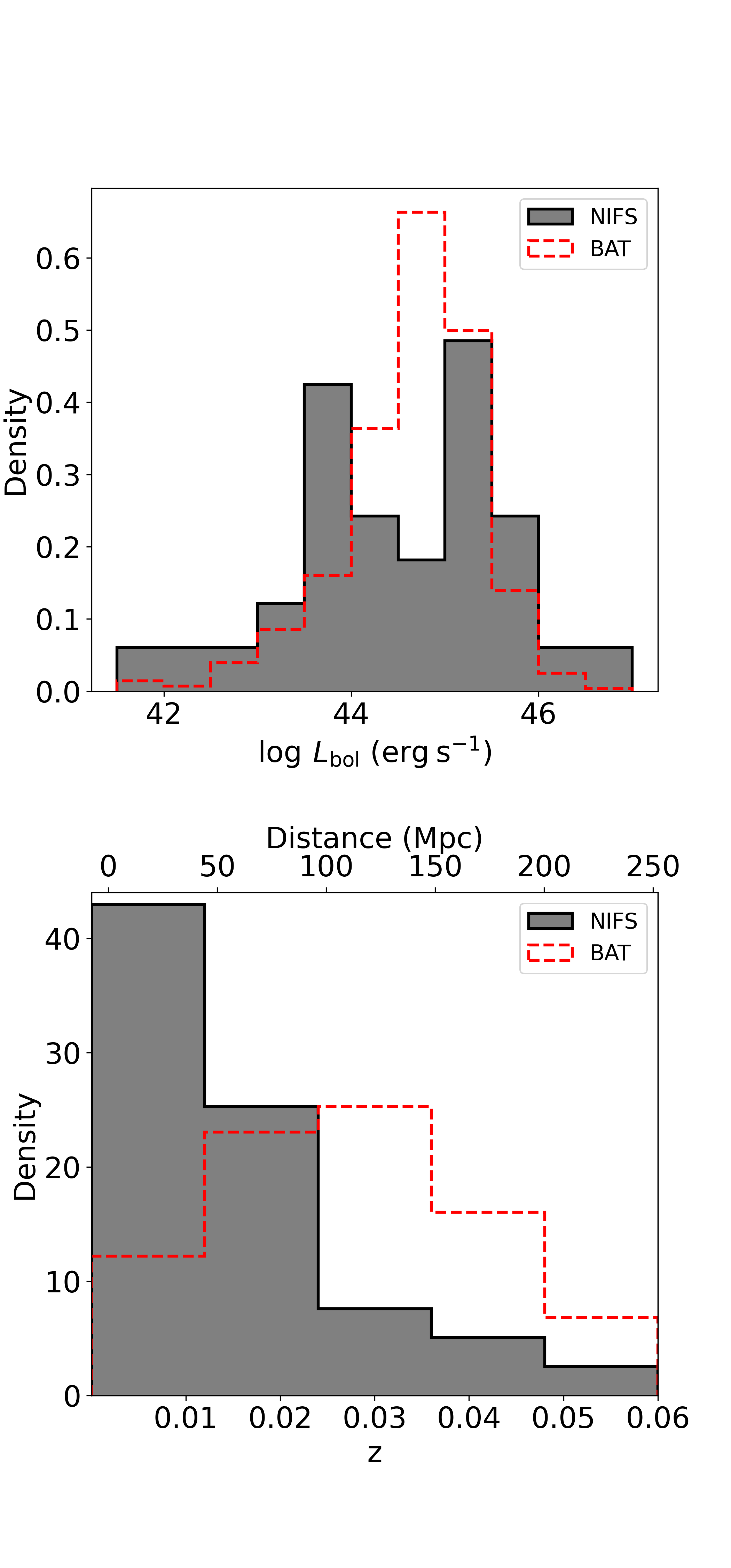
Figure 1: AGN bolometric (top) and redshift (bottom) distribution of our sample (gray) and BAT survey (red; Oh et al., 2018) for the same redshift range.

The data were obtained with the Gemini NIFS (McGregor et al., 2003), which has a square field of view of 3$\times$3 arcsec². The angular resolution of the observations is in the range 0$\aas@@fstack{\prime\prime}$11–0$\aas@@fstack{\prime\prime}$44 and velocity resolution of $\sigma_{\rm inst}\sim$20 km s^-1 (see Riffel et al., 2018b, 2021b). The data reduction followed the standard procedures, as described in Riffel et al. (2017), resulting in a single datacube for each galaxy at angular sampling of 0$\aas@@fstack{\prime\prime}$05$\times$0$\aas@@fstack{\prime\prime}$05. More details about the sample, observational strategy and data reduction can be found in Riffel et al. (2017, 2018b, 2021b).

2.2 Measurements

We characterise the hot molecular and ionised gas kinematics by measuring the $W_{\rm 80}$, $V_{\rm peak}$ and $V_{\rm cen}$ parameters for the H${}_{2}\>2.1218\,\mu$m and Br$\gamma$ emission lines, respectively. The $W_{\rm 80}$ is defined as the smalest width of the line that contains 80 per cent of its total flux and has been used to look for signatures of ionised gas outflows in AGN hosts (Zakamska & Greene, 2014; McElroy et al., 2015; Wylezalek et al., 2017; Wylezalek et al., 2020; Riffel et al., 2020; Kakkad et al., 2020). $V_{\rm peak}$ is the velocity corresponding to the peak of the emission line, which is expected to trace emission from gas in the galaxy disc, while $V_{\rm cen}$ is the centroid velocity, which is expected to be different from $V_{\rm peak}$ for asymmetric profiles. These properties are computed by using the fits of the spectra performed by Riffel et al. (2021b) using the ifscube code (Ruschel-Dutra, 2020; Ruschel-Dutra et al., 2021), where the H${}_{2}\>2.1218\,\mu$m and Br$\gamma$ emission lines are represented by up to three Gaussian components and the underlying continuum is reproduced by a first order polynomial function. The measurements of $W_{\rm 80}$ and $V_{\rm cen}$ are also obtained with the ifscube code, while $V_{\rm peak}$ is obtained directly from the modelled spectra by computing the velocity corresponding to the maximum flux value within a spectral window of 1500 km s^-1 centred at the peak of each emission line.

In Fig. 2 we present examples of the resulting line flux and kinematic maps. Besides the maps for $W_{\rm 80}$, $V_{\rm peak}$ and $V_{\rm cen}$ for H${}_{2}\>2.1218\,\mu$m and Br$\gamma$, we also present the flux maps for these emission lines, obtained by integrating the line profiles within a spectral window of 1500 km s^-1 centred at each emission line and a continuum image in the K-band – already presented in Riffel et al. (2021b), as well as maps identifying the KDRs and virially-dominated region (VDRs; see Sec. 3). In the bottom row of Fig. 2 we also present histograms for the distributions of $W_{\rm 80}$ values and residual velocities, $V_{\rm res}$, defined as $V_{\rm res}=V_{\rm cen}$-$V_{\rm peak}$ for both emission lines, as well as representative line profiles that will be discussed in the forthcoming sections. In all maps, we masked out regions where the peak of the line profile is not above 3 times the noise in the neighbouring continuum. These regions are shown as grey areas in the maps.

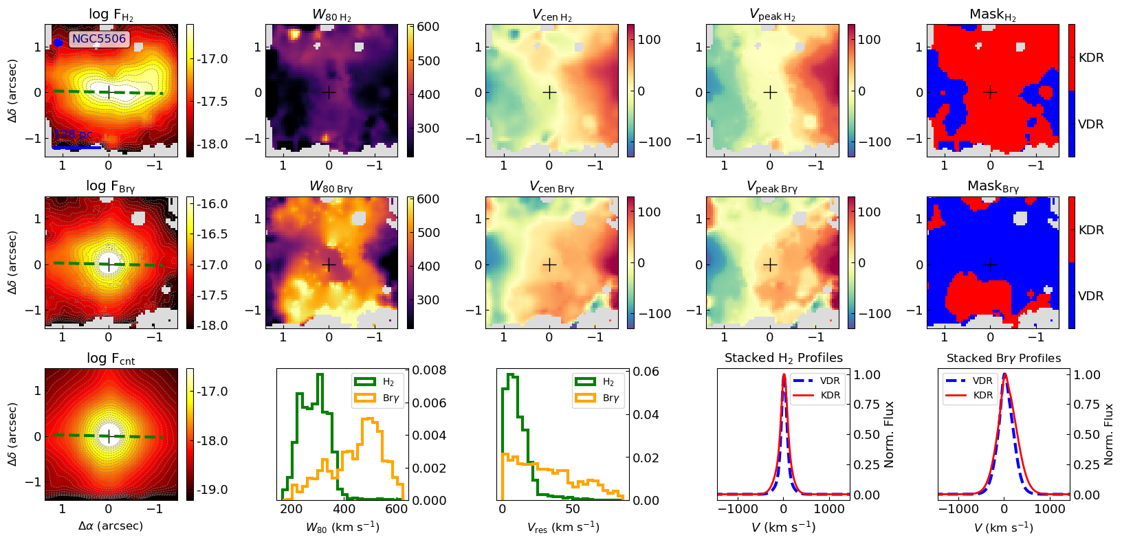
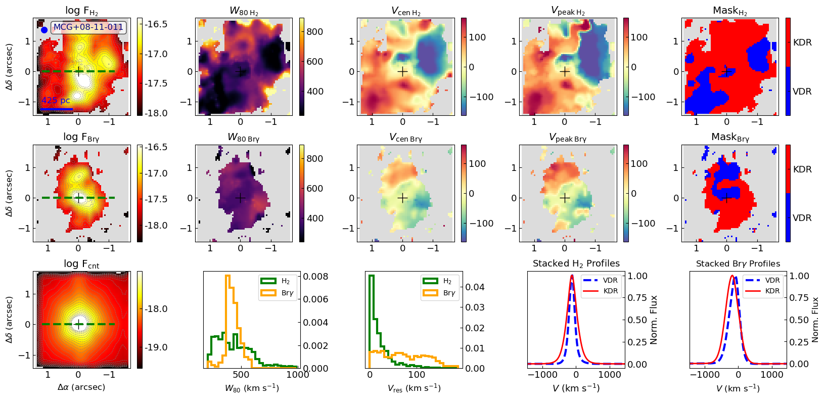
Figure 2: Examples of maps for NGC 5506 (top panels) and MCG+08-11-011 (bottom panels). For each galaxy, the first row shows the results for the H${}_{2}\>2.1218\,\mu$m  and second row show results for the the Br$\gamma$ emission line. From left to right: emission line flux distribution, $W_{\rm 80}$, $V_{\rm cen}$, $V_{\rm peak}$, and a “kinematic map” identifying the kinematically disturbed region (KDR) in red and the virially-dominated region (VDR) in blue. The colour bars show fluxes in erg s^-1 cm^-2 spaxel^-1 and velocities in km s^-1. The grey areas identify locations where the emission-line amplitude is below 3 times the continuum noise amplitude (3$\sigma$). The bottom rows show a K-band continuum image in erg s^-1 cm^-2 Å^-1 spaxel^-1, the density distributions of $W_{\rm 80}$ and $V_{\rm res}=|V_{\rm cen}-V_{\rm peak}|$ and stacked profiles of the H₂ and Br$\gamma$ emission lines from the VDR and KDR. Stacked profiles for the KDR are presented only if it corresponds to at least 10 per cent of the spaxels with detected emission. The green dashed lines in the leftmost panels show the orientation of the major axis of the large-scale disk, as presented in Riffel et al. (2021b). In all maps, North is up and East is to the left.

3 The kinematically disturbed region – KDR

Ionised outflows have been extensively studied in AGN hosts, mostly by using the [O iii]$\lambda$5007 emission line as its tracer (e.g. Zakamska & Greene, 2014; Wylezalek et al., 2017; Wylezalek et al., 2020; Riffel et al., 2020; Kakkad et al., 2020; Ruschel-Dutra et al., 2021). The $W_{\rm 80}$ parameter can be used to identify the KDR, defined as the region where the AGN significantly affects the gas kinematics (e.g through AGN winds or in situ acceleration of the clouds via radiation pressure). Usually $W_{\rm 80}>$600 km s^-1, observed in the [O iii]$\lambda$5007 line is associated with ionised outflows in quasars (e.g. Kakkad et al., 2020), while in lower luminosity AGN hosts $W_{\rm 80}>$500 km s^-1 may already be tracing the KDR emission and consistent with radiatively or mechanically driven AGN outflows (e.g. Wylezalek et al., 2020). The justification for the choice of this threshold is that even for the deepest galaxy gravitational potential of the most massive galaxies, normal orbital velocities and velocity dispersions correspond to lower $W_{\rm 80}$ values.

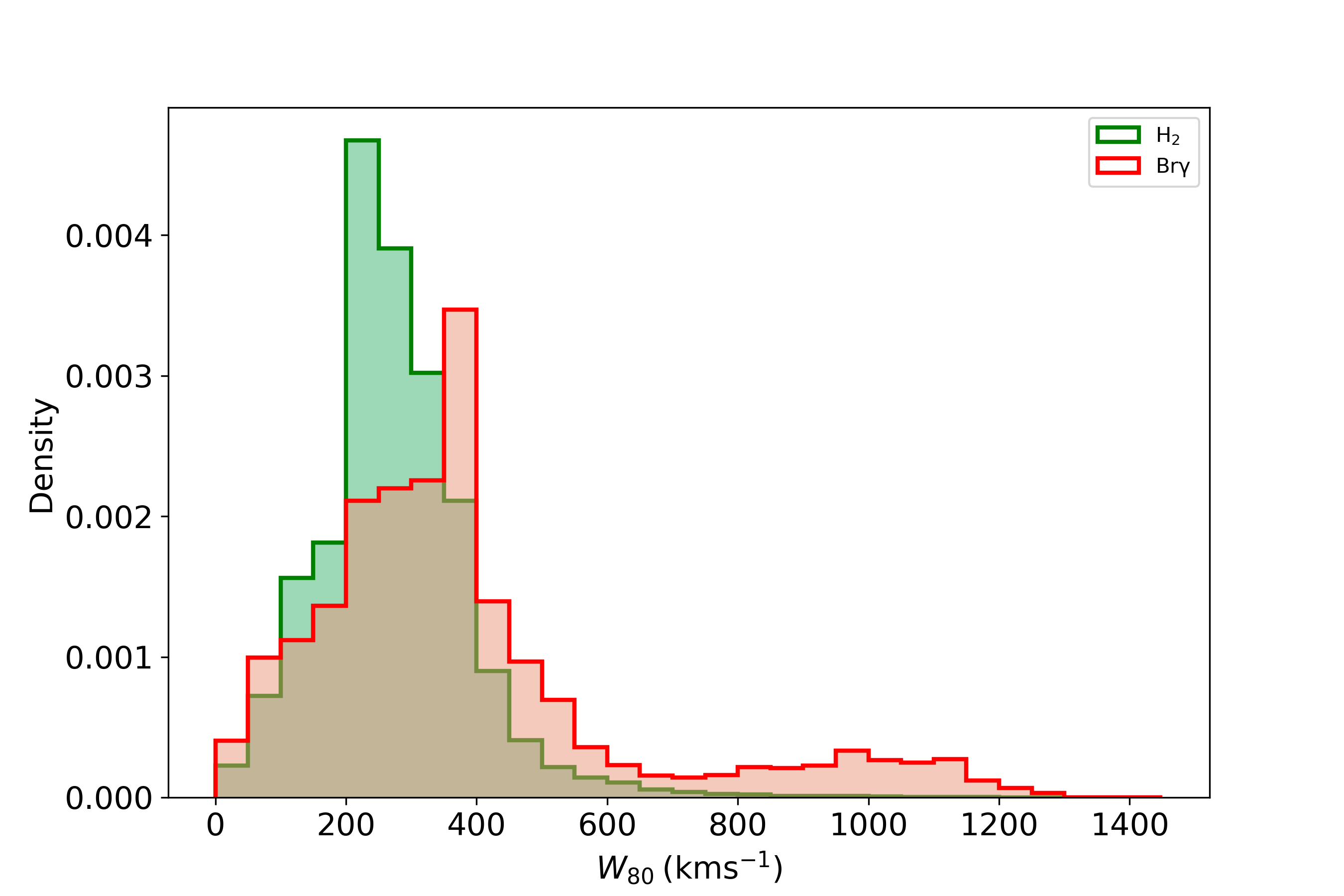
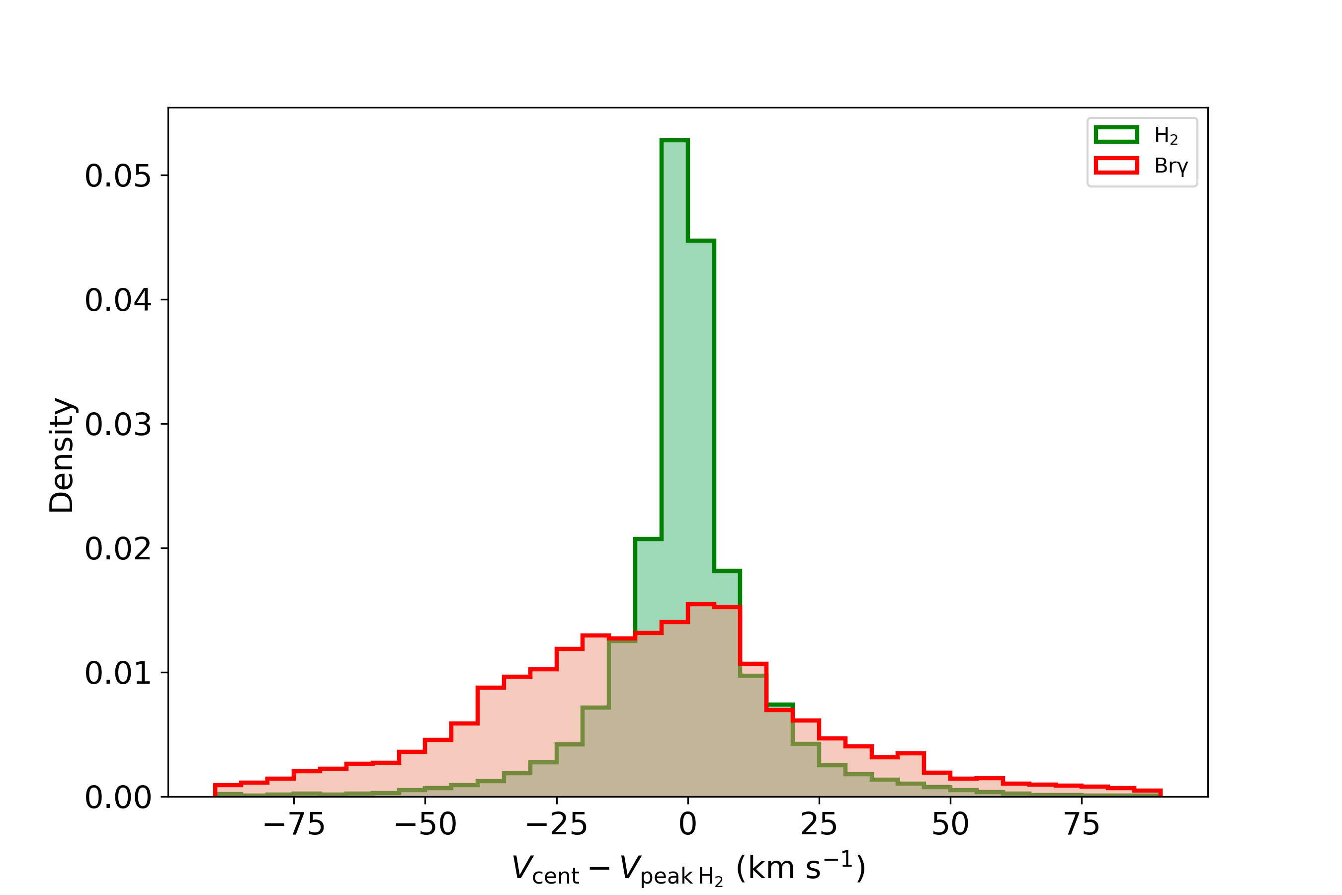
Figure 3: Left: Br$\gamma$ (in red) and H${}_{2}\>2.1218\,\mu$m (in green) $W_{\rm 80}$ distributions for our sample in bins of 50 km s^-1 using measurements in all spaxels. Right: Br$\gamma$ (in red) and H${}_{2}\>2.1218\,\mu$m (in green) residual centroid velocity distributions for our sample in bins of 5 km s^-1.

The $W_{\rm 80}$ cuts mentioned above are determined using the [O iii]$\lambda$5007 emission as a tracer of the KDR, and different cuts may be used for distinct tracers, considering the multiple gas phases in the KDR. The Br$\gamma$ emission line is more sensitive to star-formation for which narrower profiles are usually observed, compared to [O iii] which is a better tracer of the highest ionization gas. Thus, if an outflow component is superimposed to a disc component, the $W_{\rm 80}$ cutoff value for Br$\gamma$ is expected to be smaller than that for [O iii]. Similarly, the H₂ near-IR emission from the inner region of nearby Seyfert galaxies originates mostly from gas rotating in the disc, also resulting in narrower line profiles compared to those from ionised gas emission lines (e.g. Riffel et al., 2018b). Figure 3 presents the $W_{\rm 80}$ distributions of the H₂ 2.1218 $\mu$m (in green) and Br$\gamma$ (in red) emission lines for our sample. Overall, higher $W_{\rm 80}$ values are observed for Br$\gamma$ than for H${}_{2}\>2.1218\,\mu$m, confirming previous results. In addition, the Br$\gamma$ $W_{\rm 80}$ distribution clearly presents a tail of high values. A less prominent tail is also observed in the H₂ distribution, but with smaller values. Furthermore, a more accurate way of identifying the KDR requires defining different $W_{\rm 80}$ thresholds not only for each line but also for each object.

For the definition of the KDR we also use the galaxies nuclear spectra to measure the emission-line and stellar kinematics. We extract an spectrum within a circular aperture of 0$\aas@@fstack{\prime\prime}$25 radius centred at the peak of the continuum emission. The size of the aperture is comparable to the angular resolution of the data (Riffel et al., 2021b) and so, the measured kinematics is representative of the nucleus of each galaxy. We measure the stellar line-of-sight velocity distribution (LOSVD) of each galaxy by fitting the CO absorption band-heads ($\sim$2.29–2.40 $\mu$m – rest wavelengths) with the penalized Pixel-Fitting ppxf method (Cappellari & Emsellem, 2004; Cappellari, 2017) using the Gemini library of late spectral type stars observed with the Gemini Near-Infrared Spectrograph (GNIRS) IFU and NIFS (Winge et al., 2009). We were able to obtain measurements of the stellar kinematics for 14 objects (Mrks 1066, 348, 607 and NGCs 1052, 1125, 1241, 2110, 3227, 3516, 4051, 4258, 4388, 5899 and 788) in our sample. For the other objects the CO absorption bands are not detected (or are too weak), mainly due to the dilution of the bands by dust emission (Burtscher et al., 2015; Riffel et al., 2017). We measure the emission-line properties using the same procedure described in the previous section, using the ifscube code.

The near-IR H₂ emission in nearby AGN hosts is usually dominated by emission of gas in rotation in the plane of the galaxy (e.g. Hicks et al., 2013; Mazzalay et al., 2014; Riffel et al., 2018b), thus the peak velocity measured from the H${}_{2}\>2.1218\,\mu$m is expected to be similar to that of the stars. Indeed, the comparison between the nuclear H₂ peak velocities and the stellar velocities show that they are consistent with an average difference of $\langle V_{\rm peak\,H_{2}}-V_{\rm stars}\rangle=-6$ km s^-1, which is within NIFS velocity resolution of $\sim$50 km s^-1, and a standard deviation of 34 km s^-1. The velocity differences are in the range from $-45\pm 13$ km s^-1 (for NGC 1241) and $70\pm 9$ km s^-1 (for NGC 1052). This indicates that both the peak H${}_{2}\>2.1218\,\mu$m velocity and stellar velocity trace the systemic velocities of the galaxies and that $V_{\rm peak\,H_{2}}$ can be used as a proxy of the bulk velocity of the virially-dominated region.

If the gas motions are dominated by the gravitational potential, it is expected that the velocity dispersion (measured here by the $W_{\rm 80}$ parameter) decreases with the distance to the nucleus, so that the nuclear value can be used as the maximum velocity dispersion that can be attributed to the gravitational potential. We fit the emission line profiles in the nuclear spectra by a single Gaussian curve. In order to minimize the inclusion of outflows in this nuclear spectrum, we restrict the centroid velocity of the Gaussian to differ by at most 50 km s^-1 from the stellar velocity (50 km s^-1 is roughly the NIFS velocity resolution – FWHM). If this condition does not apply, we include another Gaussian component in the fit and adopt as representative of the orbital motion the one with centroid velocity closer to the stellar one. For galaxies with no stellar kinematics measurements, we use the peak H${}_{2}\>2.1218\,\mu$m velocity as reference. If the line profile is well reproduced by a single Gaussian function, we use its $W_{\rm 80}$ plus the corresponding uncertainty as a threshold to define the KDR. Spaxels with $W_{\rm 80}$ values larger than this threshold are associated to the KDR, while spaxels with smaller values are attributed to virialized gas motions, corresponding to the VDR. In Fig. 4 we present examples of the line profile fits and in Table 1 we show the maximum $W_{\rm 80}$ values attributed to motions under the gravitational potentials for each galaxy.

Table 1: $W_{\rm 80}$ values for the disc component in our sample (see text) for an aperture of 0$\aas@@fstack{\prime\prime}$25 radius centred at the peak of the continuum emission. (1) Object, (2) Number of Gaussian functions used to represent the H${}_{2}\>2.1218\,\mu$m emission line, (3) $W_{\rm 80}$ measured for the H₂ from the Gaussian component that represents the disc and (4) its uncertainty. (5)–(7) Same as (2)–(4), but for the Br$\gamma$ emission line. We consider spaxels with $W_{\rm 80}$ values larger than the nuclear values plus their uncertainties as a signature of kinematically disturbed gas. For objects with no nuclear emission, we adopt a $W_{\rm 80}$ threshold of 500 km s^-1 as a lower limit to identify the KDR, following Wylezalek et al. (2020). We identify these objects with the superscript ^∗.

(1)	(2)	(3)	(4)	(5)	(6)	(7)
	H${}_{2}\>2.1218\,\mu$m			Br$\gamma$
Type 2
NGC788	1	197	30	2	227	29
NGC1052	1	345	36	1	329	65
NGC1068	1	200	50	1	444	68
NGC1125	2	212	37	2	228	30
NGC1241	1	262	29	1	305	41
NGC2110	2	347	47	2	230	61
NGC4258	1	294	47	1	521	52
NGC4388	1	226	28	1	220	29
NGC5506	1	197	42	2	580	33
NGC5899	1	239	26	2	366	43
Mrk3	2	275	55	2	330	47
Mrk348	2	156	54	2	167	69
Mrk607	3	237	43	3	350	43
Mrk1066	1	232	26	2	222	27
ESO578-G009	–	500∗	–	–	500∗	–
Cygnus A	2	365	35	2	551	42
Type 1
NGC1275	3	408	26	2	412	45
NGC3227	2	224	34	2	356	42
NGC3516	2	193	54	1	220	53
NGC4051	1	158	32	2	211	38
NGC4151	1	355	91	1	393	41
NGC4235	1	371	52	–	500∗	–
NGC4395	1	84	24	1	101	25
NGC5548	1	311	46	2	384	64
NGC6814	1	161	30	2	291	43
Mrk79	1	315	48	1	250	53
Mrk509	–	500∗	–	–	500∗	–
Mrk618	1	199	46	1	360	43
Mrk766	1	155	38	2	169	32
Mrk926	2	201	52	2	382	52
Mrk1044	–	500∗	–	–	500∗	–
Mrk1048	2	191	44	1	148	47
MCG+08-11-011	1	279	43	1	445	43

In some cases, instead of a significant enhancement of the gas velocity dispersion, an outflow produces only a deviation of the centroid velocity of the gas with respect to that corresponding to the galaxy rest frame. This may occur, for instance, in a bipolar outflow launched from the galaxy nucleus at an angle almost perpendicular to the galaxy disc, so that the outflow just weakly interacts with the gas in the disc (e.g. Riffel et al., 2013a; Bianchin et al., 2022). In order to account for this possibility, we consider that the $V_{\rm peak}$ parameter traces virially-dominated motion and compute the residual velocity $V_{\rm res}=|V_{\rm cen}-V_{\rm peak}|$. As the H₂ is a better tracer of the emission of the disc, we use the $V_{\rm peak}$ measured for the H${}_{2}\>2.1218\,\mu$m to compute the $V_{\rm res}$ for both lines. If $V_{\rm res}>{\rm 50\>km\,s^{-1}}$, we assume that the gas motions are not dominated by the gravitational potential. We point out that only a few spaxels are selected using this criteria. The fraction of spaxels with $V_{\rm res}>{\rm 50\>km\,s^{-1}}$ correspond to only 1 percent of the total number of spaxels for the H₂ and about 4 percent for the Br$\gamma$.

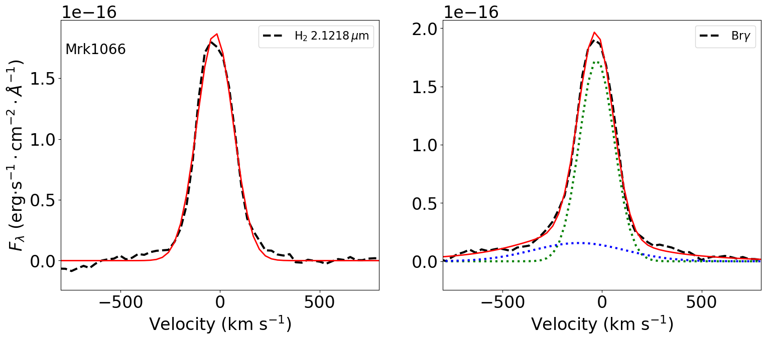
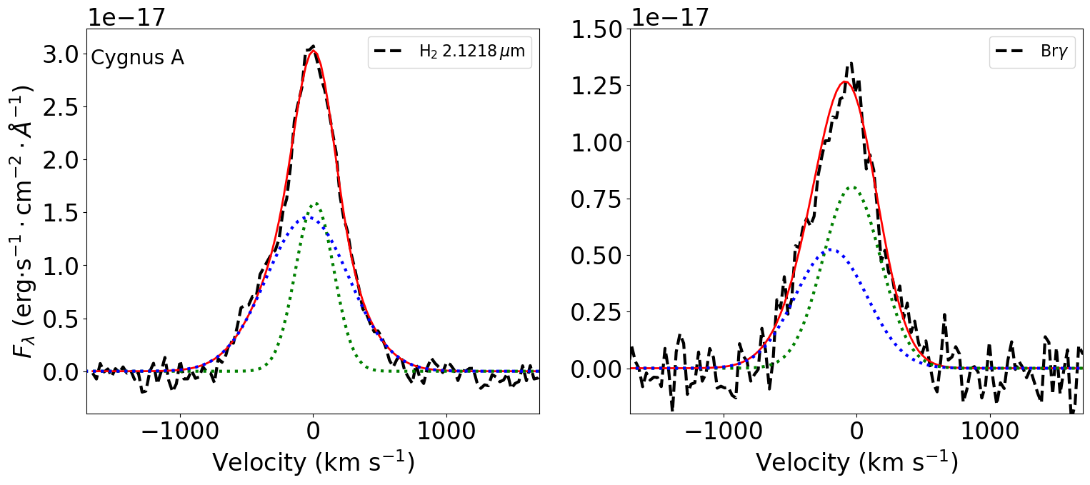
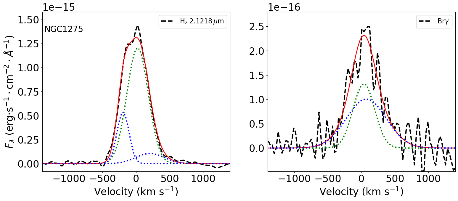
Figure 4: Examples of fits of the nuclear emission-line profiles, within an aperture of 0$\aas@@fstack{\prime\prime}$25 radius. Left panels show the fits of the H${}_{2}\>2.1218\,\mu$m and right panels show results for the Br$\gamma$ for Mrk 1066 (top), Cygnus A (middle) and NGC 1275 (bottom). The observed profiles are shown in black and the best-fit model in red. If more than one Gaussian function is used to represent the line profile, the dotted green line shows the component attributed to VDR, while the blue dotted lines represents the KDR emission.

In summary, throughout this paper, locations where $W_{\rm 80}$ are larger than the values listed in Table 1 plus their uncertainties or $V_{\rm res}>{\rm 50\>km\,s^{-1}}$ are identified as the gas KDR. The KDR is assumed to be produced by outflows. Other regions are identified as the VDRs. In the next section we derive the outflow properties and discuss their uncertainties.

4 Properties of the outflows

The origin of the KDR in central region of AGN hosts may be due to gas outflows (e.g. Wylezalek et al., 2020; Ruschel-Dutra et al., 2021; Deconto-Machado et al., 2022) and thus, we can use the flux and kinematic measurements to determine the properties of the hot molecular and ionised gas outflows, traced by the H₂ and Br$\gamma$ emission lines, respectively. In the two-bottom right panels for each galaxy in Fig. 2 we present stacked emission line profiles for the KDR (in red) and VDR (blue). These profiles were constructed by summing up all spaxels of each region using the peak velocity of the line as reference. Such profiles are shown for all objects in the supplementary material. In order to avoid possible spurious measurements, we only plot the stacked profile for the KDR if this region corresponds to at least 10 per cent of the spaxels with detection of the corresponding emission line. As expected (by definition) the profiles from the KDR are broader and in several cases present distinctly different peak velocities than those from the VDR.

We find that 31 galaxies (94 per cent) present at least 10 per cent of the spaxels in the KDR considering only spaxels with detected Br$\gamma$ emission. For the H₂, the number of objects with more than 10 per cent of the spaxels in the KDR is 25 (76 per cent). We estimate the outflow properties only for these objects, in each gas phase.

4.1 Estimates of the outflows properties

We estimated the mass of hot H₂ and H ii using the fluxes of the H${}_{2}\>2.1218\,\mu$m and Br$\gamma$ emission lines, respectively. The mass of hot molecular gas can be derived by

$$\left(\frac{M_{\rm H_{2}}}{M_{\odot}}\right)=5.0776\times 10^{13}\left(\frac{F_{\rm H_{2}\,2.1218}}{\rm erg\,s^{-1}\,cm^{-2}}\right)\left(\frac{D}{\rm Mpc}\right)^{2},$$ (1)

where $F_{\rm H_{2}\,2.1218}$ is the H${}_{2}\,2.1218\mu$m emission-line flux and $D$ is the distance to the galaxy. Local thermal equilibrium is assumed with an excitation temperature of 2000 K (e.g. Scoville et al., 1982; Riffel et al., 2014).

The mass of ionised gas is obtained by

$$\left(\frac{M_{\rm H\,II}}{M_{\odot}}\right)=3\times 10^{19}\left(\frac{F_{\rm Br\gamma}}{\rm erg\,cm^{-2}\,s^{-1}}\right)\left(\frac{D}{\rm Mpc}\right)^{2}\left(\frac{N_{e}}{\rm cm^{-3}}\right)^{-1},$$ (2)

where $F_{\rm Br\gamma}$ is the Br$\gamma$ flux and $N_{e}$ is the electron density (Osterbrock & Ferland, 2006; Storchi-Bergmann et al., 2009). We adopt an electron density of $N_{e}=1000\,{\rm cm^{-3}}$, which is a typical value measured in AGN hosts from the [S ii]$\lambda\lambda$6717,6730 lines (e.g. Dors et al., 2014, 2020; Brum et al., 2017; Freitas et al., 2018; Kakkad et al., 2018).

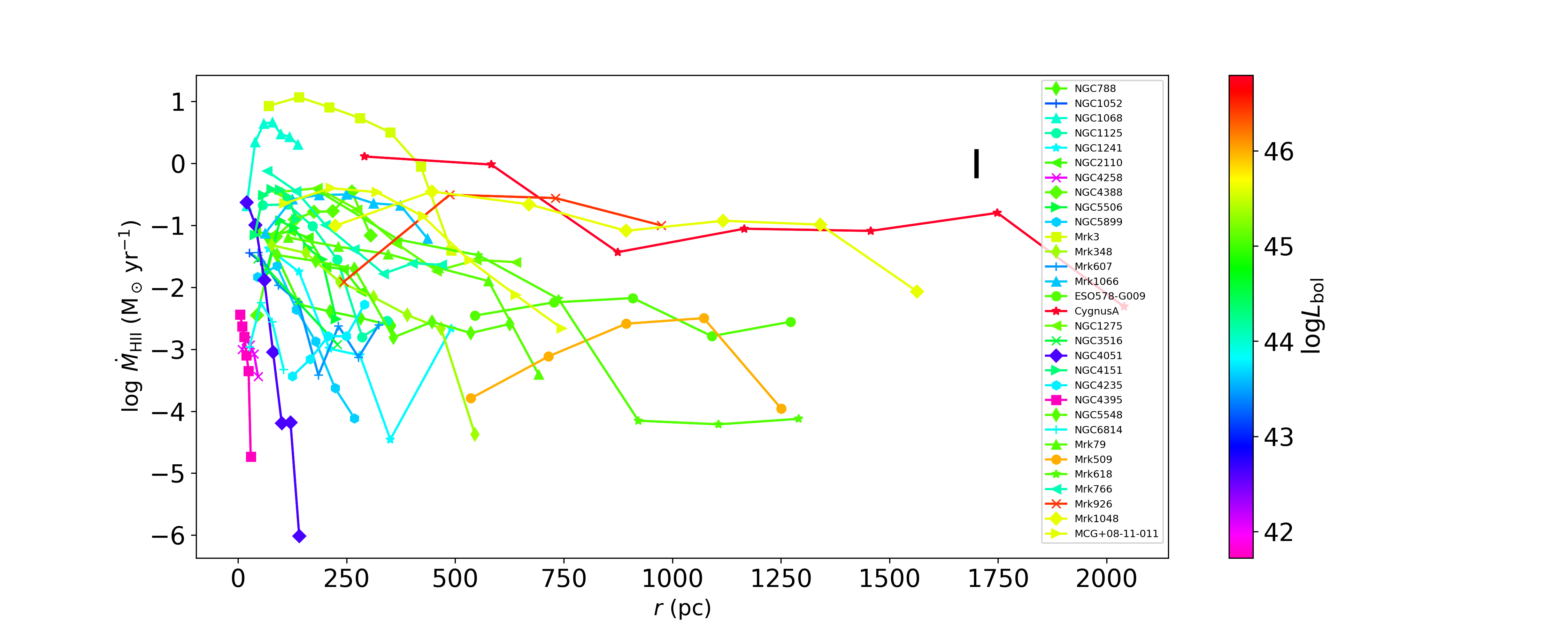
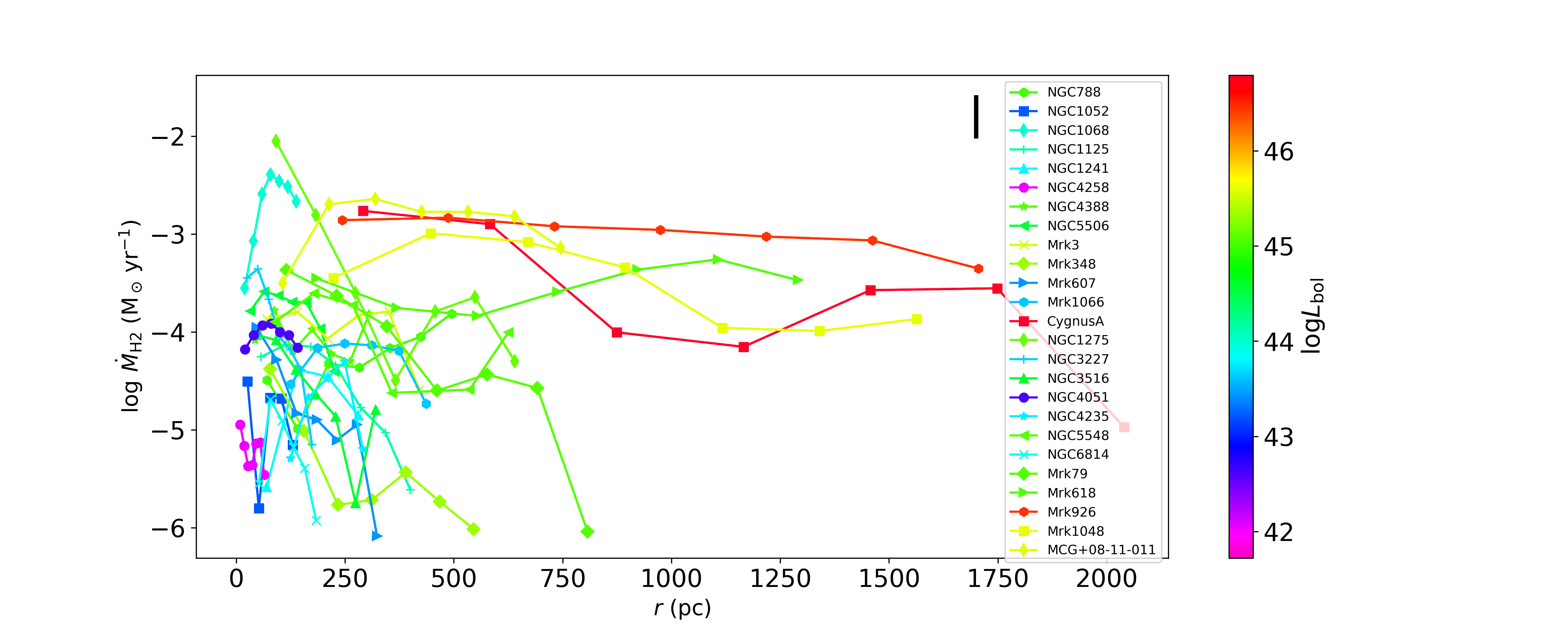
Figure 5: Radial profiles of the mass-outflow rates in ionised (top) and hot molecular (middle) gas for the galaxies in our sample with detected outflows. The vertical bar in the top-right corner shows typical uncertainties in the mass-outflow rates. The bottom panel show radial profiles of the normalized ratio between the ionised and molecular outflow rates, plus an arbitrary constant, for objects with outflows in both phases. All profiles are colour coded by the AGN bolometric luminosity, as indicated by the colour bars.

Many assumptions are needed to estimate the properties of outflows, which can lead to different results. These properties are affected mainly by the choice of geometries and densities (e.g. Harrison et al., 2018; Baron & Netzer, 2019; Lutz et al., 2020; Kakkad et al., 2020, 2022; Davies et al., 2020; Ruschel-Dutra et al., 2021; Revalski et al., 2021, 2022). Here, we estimate the mass of the gas in the outflow ($M_{\rm out}$) by

$$M_{\rm out}=\sum_{i}M_{\rm out}^{i},$$ (3)

where the sum is done over all spaxels whose emission is dominated by the outflow as defined above and $M_{\rm out}^{i}$ is the mass of the outflow calculated for each spaxel $i$, using Eqs. 1 and 2 for the molecular and ionised gas, respectively. Following Ruschel-Dutra et al. (2021), to compute the masses of the gas in the outflow, instead of using the total flux of the emission lines from the spaxels in the KDR ($F_{\rm KDR}$), we use only the fraction of the flux corresponding to absolute velocities larger than $W_{\rm 80}/2$ from the peak velocity. Then, we characterise the outflows in two different ways: (i) adopting a spherical shell geometry and (ii) obtaining radial profiles of the properties and then using them to estimate their peak values. These outflow properties are calculated as follows:

i. Spherical geometry: Global outflow properties
In this method, we estimate the global or integrated outflow properties.

• Velocity of the bulk of the outflow ($V_{\rm out}$), defined as

  $$V_{\rm out}=\frac{\langle W_{\rm 80\>KDR}F_{\rm KDR}\rangle}{\langle F_{\rm KDR}\rangle},$$ (4)

  which is an average velocity over the region dominated by outflows where $W_{\rm 80\>KDR}$ and $F_{\rm KDR}$ are the $W_{\rm 80}$ values and fraction of the flux corresponding to absolute velocities larger than $W_{\rm 80}/2$ from the peak velocity of the corresponding emission lines for spaxels in the KDR.

• Radius of the bulk of the outflow ($R_{\rm out}$), defined as

  $$R_{\rm out}=\frac{\langle R_{\rm KDR}F_{\rm KDR}\rangle}{\langle F_{\rm KDR}\rangle},$$ (5)

  where $R_{\rm KDR}$ are the distances of outflow-dominated spaxels from the galaxy’s nucleus.

• Mass outflow rate computed by assuming a spherical geometry ($\dot{M}_{\rm out}^{\rm b}$), given by

  $$\dot{M}_{\rm out}^{\rm b}=\frac{M_{\rm out}V_{\rm out}}{R_{\rm out}}.$$ (6)

• Kinetic power of the outflow for a spherical geometry ($\dot{E}_{\rm out}^{\rm b}$), given by

  $$\dot{E}_{\rm out}^{\rm b}=\frac{1}{2}\dot{M}_{\rm out}^{\rm b}V_{\rm out}^{2}.$$ (7)

ii. Radial profiles: peak outflow properties

In this method, we calculate the properties as a function of distance from the nucleus and adopt as mass outflow rate and power their peak values. We compute the mass-outflow rates within circular apertures of 0$\aas@@fstack{\prime\prime}$25 width centred at the nucleus considering only spaxels whose line emission are dominated by the outflow component. For each shell, the mass rate [$\dot{M}_{\rm out}^{\rm sh}(r)$] and kinetic power [$\dot{E}_{\rm out}^{\rm sh}(r)$] of the outflow are computed by:

$$\dot{M}_{\rm out}^{\rm sh}(r)=\frac{M_{\rm out}^{\rm sh}V_{\rm out}^{\rm sh}}{\Delta\,R},$$ (8)

and

$$\dot{E}_{\rm out}^{\rm sh}(r)=\frac{1}{2}\dot{M}_{\rm out}^{\rm sh}(r)(V_{\rm out}^{\rm sh})^{2},$$ (9)

respectively. In these equations, $r$ corresponds to the distance of the centre of the shell from the nucleus, $M_{\rm out}^{\rm sh}$ is the mass of the gas in the outflow in the shell obtained using Eqs. 1 and 2 and $V_{\rm out}^{\rm sh}$ is the outflow velocity defined as the median of the $W_{\rm 80}$ values within the shell, and $\Delta\,R$ is the width of the shell (0$\aas@@fstack{\prime\prime}$25). Then, we define the outflow properties using the parameters below.

• Radius corresponding to the peak of the outflow ($R_{\rm peak}$): The $R_{\rm peak}$ is defined as the radius where the mass-outflow rate radial profile reaches its maximum value. In Fig. 5 we present the resulting radial profiles for the ionised and molecular gas mass outflow rate.

• Maximum value of the mass-outflow rate ($\dot{M}_{\rm peak}$): defined as the peak of the values computed within circular apertures of 0$\aas@@fstack{\prime\prime}$25 width (i.e. the maximum value of $\dot{M}_{\rm out}^{\rm sh}$).

• Maximum value of the kinetic power of the outflow ($\dot{E}_{\rm peak}$): defined as the peak of the values computed circular apertures of 0$\aas@@fstack{\prime\prime}$25 width (i.e. the maximum value of $\dot{E}_{\rm out}^{\rm sh}$).

In Figure 5 we present the radial profiles of the mass-outflow rates in ionised (top panel) and hot molecular (bottom panel) gas. For most galaxies, the radial distribution of the mass outflow rates in both molecular and ionised gas shows an increase with radius from the nucleus until reaching a maximum value at $R_{\rm peak}$, then decreasing with radius. A similar behaviour was obtained by Revalski et al. (2021) for six luminous Seyfert galaxies (including NGC 1068, NGC 4151 and Mrk 3) based on observations of the [O iii] emission line using long slit spectra obtained with the Space Telescope Imaging Spectrograph (STIS) and accurate determinations of radial density profiles.

4.2 Uncertainties

The uncertainties in the properties of AGN outflows are usually high because of the number of assumptions that have to be made to estimate them, such as the geometry, the electron density and velocity of the outflow. The electron density represents one of the major source of uncertainties in computing the mass-outflow rates in ionised gas due to different assumptions or tracers used to measure it. Depending on tracer of the electron density used, uncertainties of approximately one order of magnitude are expected for the derived mass outflow rates, as extensively discussed in recent works (e.g. Baron & Netzer, 2019; Davies et al., 2020; Revalski et al., 2022).

The electron density in the AGN narrow line region is a strong function of the distance to the nucleus and calculating the masses of ionized gas require multicomponent photoionization models to reproduce the observed emission-line intensities, as done by Revalski et al. (2022) for a sample of nearby Seyfert galaxies using HST STIS spectra. These authors found that using a constant density value of 10² cm^-3 overestimates the mass of ionised gas, while adopting a value of 10³ cm^-3 results in an agreement within $\pm$1 dex between the masses estimated from H recombination lines and those obtained from photoionization models. As mentioned above, in this work we adopt $N_{e}=1\,000\,{\rm cm^{-3}}$, which is a typical value for AGN hosts using the [S ii] doublet (e.g. Dors et al., 2014, 2020; Perna et al., 2017; Freitas et al., 2018; Kakkad et al., 2018), and thus the expected uncertainty regarding the density choice is $\sim$1 dex in the outflow properties.

The uncertainty associated to the geometry of the outflow is smaller, with distinct geometries (e.g. conical and shells) resulting in overall similar values of the mass-outflow rates, and with typical standard deviations of the differences of $<$0.5 dex between the estimates using distinct geometries (e.g. Kakkad et al., 2022).

Another source of uncertainty in the estimate of outflow properties using spatially resolved observations is associated to the selection criteria of the outflow dominated spaxels and the emission-line fluxes used to compute the mass of gas in the outflow. In order to estimate the effect of different assumptions, we estimate the global mass outflow rates using three sets of assumptions. The assumptions are the following: Method 1 – we assume that spaxels with $W_{\rm 80}$ larger than the values presented in Tab. 1 are associated to outflows as in the calculation described in Sec. 4 (which we will refer to as the adopted method for comparison purposes), but we use the total line flux of the spaxel instead of only the fluxes of its wings as done in Sec. 4. A fraction of the emission-line flux may be due to the emission of the gas in the disc (at lower velocities), resulting in an overestimation of the gas mass in the outflow. Thus, method 1 likely results in upper limits for the outflow properties. Method 2 – the spaxels corresponding to outflows are selected using a single $W_{\rm 80}$ threshold of 500 km s^-1 as defined by Wylezalek et al. (2020), and the total flux of the line in each spaxel is used to compute the mass of gas. Method 3 – the same $W_{\rm 80}$ threshold of method 2 is used, and the mass of ionized gas is calculated using the flux corresponding to absolute velocities larger than $W_{\rm 80}/2$ from the peak velocity of the corresponding emission line. These assumptions will likely result in a lower limit of the mass outflow rate, as it does not include lower velocity outflows.

In Figure 6, we present the comparison among the mass-outflow rates in ionized (left) and hot molecular (right) gas derived using the different set of assumptions, for each object. The mean differences between the maximum and minimum values are 1.0$\pm$0.5 dex for the ionized gas and 0.7$\pm$0.4 dex for the hot molecular gas. The highest discrepancies are of about two orders of magnitude for the ionized gas and one order of magnitude for the molecular gas, with the adopted method resulting in values between the maximum and minimum estimates for most objects.

With these caveats in mind, we summarise the outflow properties and compare with values available in the literature, most of which share the same sources of uncertainty in measurements as ours.

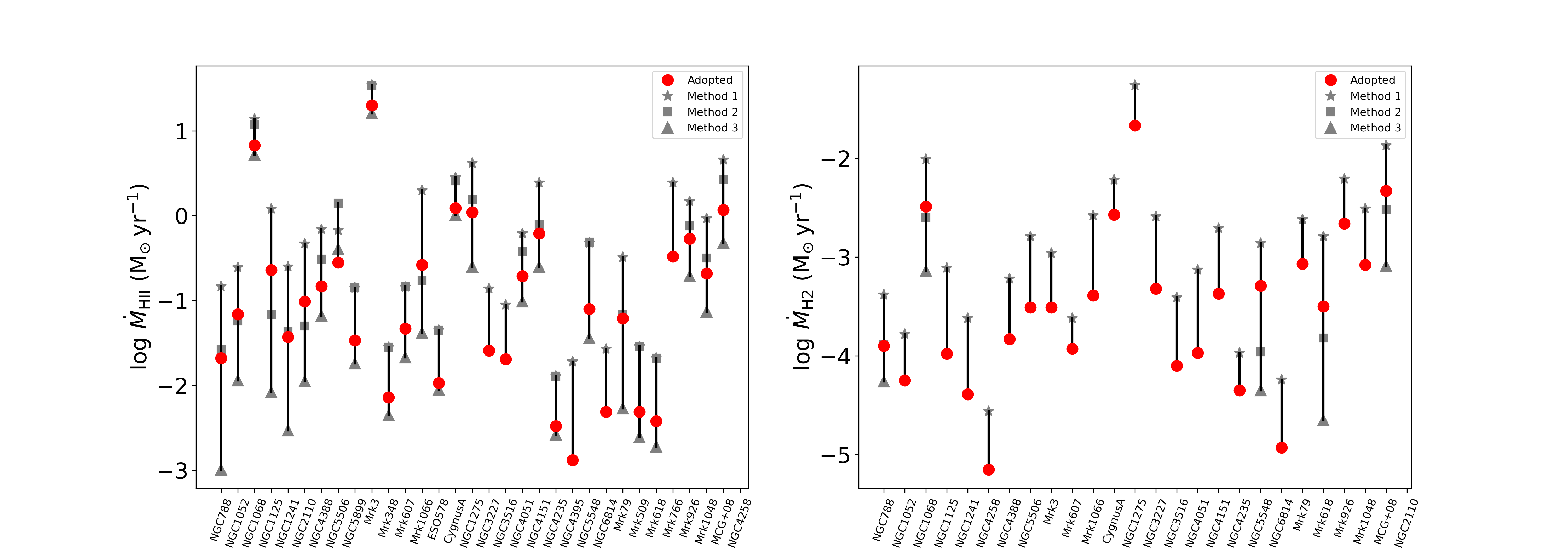
Figure 6: Comparison of the global mass outflow rates in ionized (left) and hot molecular (right) gas obtained using different assumptions (see Sec. 6).

4.3 Summary of derived outflow properties and comparison with the literature

In Tables 2 and 3 we present the derived properties of the ionised and molecular outflows, respectively. The uncertainties in the outflow parameters quoted in the table are estimated by propagating the uncertainties in the fluxes of the H${}_{2}\>2.1218\,\mu$m and Br$\gamma$ emission lines, the uncertainties in the radius (estimated as the the standard error of the radii of individual spaxels in the KDR) and velocity of the outflow (estimated as the standard error of $W_{\rm 80}$ values in the KDR). This uncertainties can be considered as lower limits, as systematic errors regarding the assumptions (e.g. densities and geometry) used to calculate the outflow properties may be the dominant source of uncertainties in deriving outflow properties, as discussed in Sec. 5. The masses of ionised gas in the outflow are in the range 10³–10⁷ M_⊙, while the molecular outflows show masses in the range 10¹–10⁴ M_⊙. Figure 7 shows the distributions of the mass fraction of the gas in the outflow relative to the total mass of molecular and ionised gas ($f_{\rm out}=M_{\rm out}/M_{\rm gas}$), obtained using Eq. 1 and 2. The mass of the gas in the outflow is estimated by considering only spaxels from the KDR, while the total gas masses are obtained by summing the contributions of all spaxels within the observed field-of-view with detected emission. For galaxies with no detected outflows, we assume $f_{\rm out}=0$. The $f_{\rm out}$ in ionised and molecular gas are listed in Tabs. 2 and 3, respectively. For most galaxies, the amount of outflowing gas corresponds to less than 30 per cent of the total gas reservoir in the central region of the galaxies, both in ionised and molecular gas.

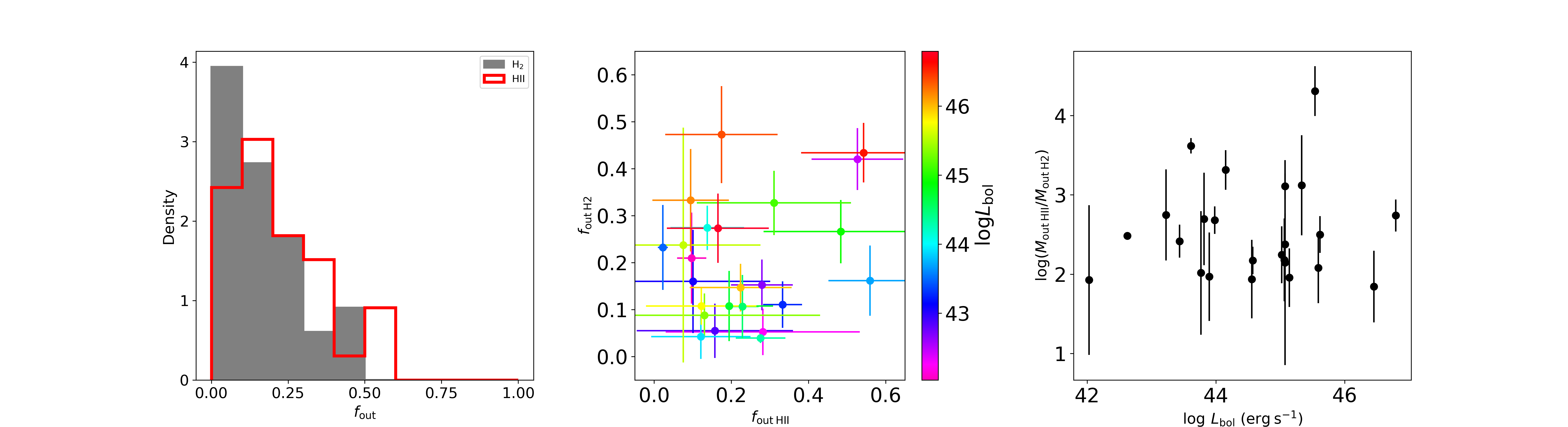
Figure 7: Left: Distribution of the fraction of gas in the outflow ($f_{\rm out}=\frac{M_{\rm out}}{M_{\rm total}}$), compared to the total masses of ionised (in red) and molecular (in grey) gas. Middle: Plot of the $f_{\rm out}$ observed in H₂ (y-axis) vs. those seen in H ii (x-axis), colour coded by the AGN bolometric luminosity. Right: Plot of the ratio of mass of ionised and molecular gas in the outflow versus the AGN bolometric luminosity.

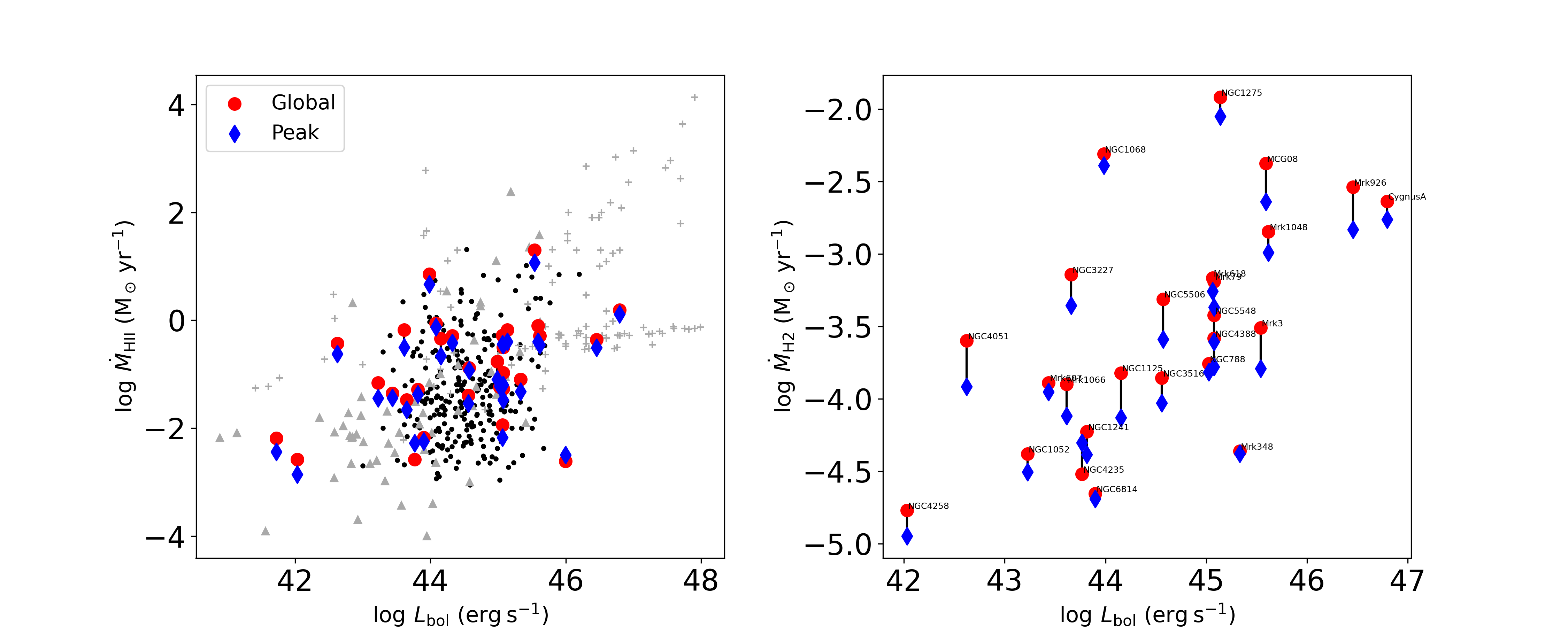
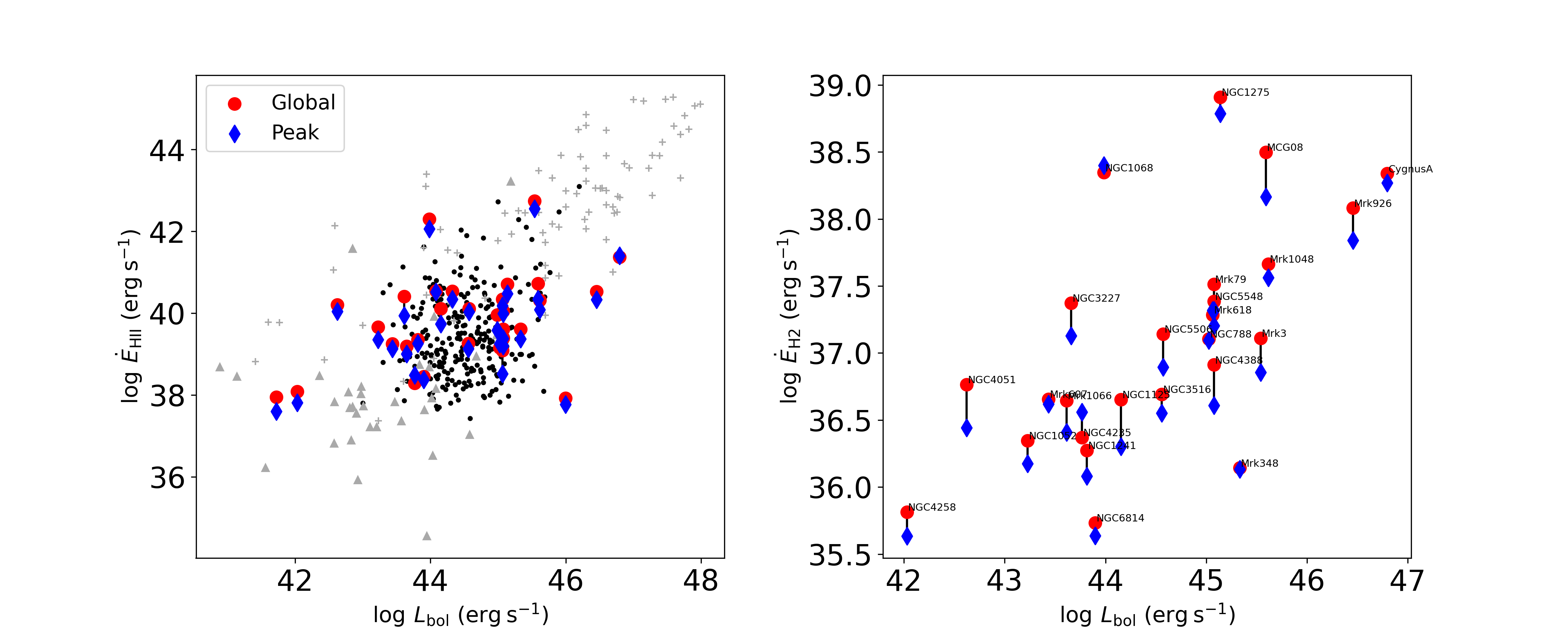
Figure 8: Top panels: plot of mass-outflow rates vs. AGN bolometric luminosity. Mass-outflow rates for the ionised (left) and hot molecular gas (right) obtained by assuming a spherical shell geometry (red circles) and peak from radial profiles (blue diamonds) are shown for each object. The grey and black points are a compilation of values from the literature, as described in the text. Bottom panels: same as top panels, but for the kinetic power of the outflows. Typical uncertainties in both parameters are 0.2 dex for both gas phases, as shown in Tabs. 2 and 3.

In the top panels of Figure 8 we show the plots of the mass outflow rates obtained for the ionised (left panel) and molecular gas against the AGN bolometric luminosity. For each object, we present estimates using the two approaches described above, for the global properties of the outflow (red circles) and peak value of the radial profile (blue diamond). The black points represent a compilation of measurements available in the literature for ionised outflows for nearby AGN, adopting various values of electron density for the outflow. These points include estimates for low luminosity AGN based on SDSS-III spectra using densities based on the ionisation parameter (Baron & Netzer, 2019), luminous Seyferts based on nuclear spectra using densities measurements from auroral and transauroral lines (Davies et al., 2020) and on long-slit HST spectra and photoionisation models (Revalski et al., 2021), and nearby QSOs based on HST spectra and photoionisation models (Trindade Falcão et al., 2021b).

As discussed in recent works, the choice of the method used to estimate the density of ionised outflows is one of the main sources of uncertainty to estimate their mass-outflow rates (Baron & Netzer, 2019; Davies et al., 2020; Revalski et al., 2022), resulting in values that can differ by approximately one order of magnitude. For example, the most common method used in the optical to estimate the electron density, based on the [S ii]$\lambda\lambda$6717,6731 doublet, provides values significantly lower than the real densities of ionised ouflows (Davies et al., 2020). In Fig. 8, we include mass-outflow rates from Ruschel-Dutra et al. (2021), Deconto-Machado et al. (2022) and Kakkad et al. (2022, for their estimates using a circular 3 arcsec diameter aperture), estimated using densities based on the [S ii] lines, measured from spatially resolved spectra. These estimates are shown as grey triangles.

Table 2: Properties of the ionised gas Outflows. (1) Name of the galaxy; (2) Adopted distance: for most galaxies, the distances are estimated from the redshift, except for except for those with accurate distance determinations: NGC 3227 (Tonry et al., 2001) , NGC 4051 (Yuan et al., 2021), NGC 4151 (Yuan et al., 2020), NGC 4258 (Reid et al., 2019), NGC 4395 (Thim et al., 2004) and NGC 6814 (Bentz et al., 2019). (3) AGN bolometric luminosity; (4) Radius of the bulk of the outflow (spherical geometry); (5) Radius of the peak of the outflow (spherical shells geometry); (6) Total mass of the outflow considering only spaxels in the KDR; (7) Mass fraction of the gas in the outflow; (8–12) Properties of the outflows estimated using the two methods described in the text.

(1)	(2)	(3)	(4)	(5)	(6)	(7)	(8)	(9)	(10)	(11)	(12)
							Global/Bulk outflow			Radial profiles
Galaxy	$D$	$\log L_{\rm bol}$	$R_{\rm out}$	$R_{\rm peak}$	$\log M_{\rm out}$	$f_{\rm out}$	$V_{\rm out}$	$\log\dot{M}_{\rm out}^{\rm b}$	$\log\dot{E}_{\rm out}^{\rm b}$	$\log\dot{M}_{\rm peak}$	$\log\dot{E}_{\rm peak}$
	[Mpc]	[${\rm erg\>s}^{-1}$]	[pc]	[pc]	[M⊙]		[${\rm km\>s}^{-1}$]	[M${}_{\odot}{\rm yr^{-1}}$]	[${\rm erg\>s}^{-1}$]	[M${}_{\odot}{\rm yr^{-1}}$]	[${\rm erg\>s}^{-1}$]
Type 2
NGC788	58.3	45.02	165$\pm$39	70$\pm$30	3.93$\pm$0.49	0.04$\pm$0.04	284$\pm$49	-1.68$\pm$0.50	38.73$\pm$0.50	-1.66$\pm$0.50	38.82$\pm$0.50
NGC1052	21.4	43.23	97$\pm$34	25$\pm$34	3.54$\pm$0.46	0.28$\pm$0.25	459$\pm$37	-1.16$\pm$0.47	39.66$\pm$0.47	-1.45$\pm$0.52	39.36$\pm$0.52
NGC1068	16.3	43.98	414$\pm$29	78$\pm$24	5.74$\pm$0.19	0.50$\pm$0.13	922$\pm$42	0.83$\pm$0.19	42.26$\pm$0.19	0.61$\pm$0.21	41.97$\pm$0.22
NGC1125	47.1	44.15	168$\pm$104	114$\pm$102	4.83$\pm$0.14	0.14$\pm$0.07	302$\pm$32	-0.64$\pm$0.24	39.82$\pm$0.24	-0.95$\pm$0.33	39.43$\pm$0.34
NGC1241	57.9	43.82	149$\pm$40	70$\pm$31	4.00$\pm$0.68	0.12$\pm$0.20	371$\pm$45	-1.43$\pm$0.68	39.21$\pm$0.68	-1.51$\pm$0.68	39.12$\pm$0.68
NGC2110	33.4	44.99	283$\pm$41	121$\pm$33	4.39$\pm$0.32	0.18$\pm$0.09	424$\pm$37	-1.01$\pm$0.32	39.75$\pm$0.32	-1.36$\pm$0.33	39.32$\pm$0.33
NGC4258	7.6	42.03	–	–	–	–	–	–	–	–	–
NGC4388	36.0	45.08	495$\pm$80	261$\pm$41	4.90$\pm$0.28	0.16$\pm$0.07	366$\pm$39	-0.83$\pm$0.29	39.80$\pm$0.29	-0.69$\pm$0.29	39.76$\pm$0.29
NGC5506	26.6	44.57	334$\pm$46	96$\pm$40	4.70$\pm$0.08	0.05$\pm$0.01	552$\pm$42	-0.55$\pm$0.10	40.44$\pm$0.10	-0.57$\pm$0.17	40.38$\pm$0.18
NGC5899	36.9	43.65	153$\pm$33	89$\pm$29	3.74$\pm$0.43	0.16$\pm$0.13	381$\pm$42	-1.47$\pm$0.44	39.19$\pm$0.44	-1.65$\pm$0.44	39.00$\pm$0.44
Mrk3	57.9	45.54	239$\pm$31	140$\pm$29	6.51$\pm$0.15	0.56$\pm$0.11	939$\pm$48	1.30$\pm$0.16	42.74$\pm$0.16	1.07$\pm$0.17	42.56$\pm$0.18
Mrk348	64.3	45.33	346$\pm$60	233$\pm$40	3.57$\pm$0.42	0.02$\pm$0.04	474$\pm$50	-2.14$\pm$0.43	38.71$\pm$0.43	-2.15$\pm$0.43	38.59$\pm$0.43
Mrk607	38.1	43.44	146$\pm$35	46$\pm$33	3.93$\pm$0.18	0.13$\pm$0.09	352$\pm$53	-1.33$\pm$0.20	39.27$\pm$0.21	-1.44$\pm$0.29	39.13$\pm$0.29
Mrk1066	51.4	43.61	365$\pm$40	249$\pm$33	5.16$\pm$0.15	0.11$\pm$0.06	374$\pm$31	-0.58$\pm$0.16	40.06$\pm$0.16	-0.85$\pm$0.17	39.62$\pm$0.17
ESO578-G009	150.0	45.06	576$\pm$178	909$\pm$78	4.26$\pm$0.53	0.04$\pm$0.05	564$\pm$143	-1.97$\pm$0.54	39.03$\pm$0.54	-2.17$\pm$0.54	38.52$\pm$0.54
CygnusA	240.4	46.80	268$\pm$41	291$\pm$39	6.19$\pm$0.25	0.28$\pm$0.10	574$\pm$45	0.09$\pm$0.25	41.11$\pm$0.25	-0.01$\pm$0.26	41.28$\pm$0.26
Type 1
NGC1275	75.4	45.14	168$\pm$50	91$\pm$49	5.52$\pm$0.35	0.28$\pm$0.16	480$\pm$46	0.04$\pm$0.36	40.90$\pm$0.36	-0.13$\pm$0.38	40.67$\pm$0.38
NGC3227	20.5	43.66	201$\pm$38	49$\pm$27	3.47$\pm$0.33	0.03$\pm$0.05	402$\pm$46	-1.59$\pm$0.34	39.12$\pm$0.34	-1.60$\pm$0.36	39.09$\pm$0.36
NGC3516	37.7	44.56	67$\pm$35	45$\pm$35	3.21$\pm$0.76	0.21$\pm$0.20	381$\pm$46	-1.69$\pm$0.76	38.97$\pm$0.76	-1.89$\pm$0.76	38.78$\pm$0.76
NGC4051	16.6	42.62	109$\pm$43	20$\pm$40	4.04$\pm$0.81	0.17$\pm$0.20	371$\pm$50	-0.71$\pm$0.42	39.93$\pm$0.31	-0.90$\pm$0.37	39.77$\pm$0.28
NGC4151	15.8	44.32	393$\pm$44	76$\pm$39	5.00$\pm$0.17	0.28$\pm$0.06	430$\pm$30	-0.21$\pm$0.18	40.56$\pm$0.18	-0.48$\pm$0.24	40.21$\pm$0.24
NGC4235	34.3	43.77	603$\pm$84	290$\pm$30	3.21$\pm$0.65	0.17$\pm$0.28	472$\pm$80	-2.48$\pm$0.65	38.37$\pm$0.65	-2.21$\pm$0.65	38.55$\pm$0.65
NGC4395	4.0	41.72	195$\pm$48	4$\pm$44	1.70$\pm$0.40	0.07$\pm$0.05	233$\pm$31	-2.88$\pm$0.41	37.36$\pm$0.41	-3.15$\pm$1.02	36.89$\pm$1.02
NGC5548	73.7	45.08	215$\pm$49	89$\pm$45	4.57$\pm$1.13	0.11$\pm$0.20	383$\pm$37	-1.10$\pm$1.13	39.56$\pm$1.13	-1.32$\pm$1.13	39.36$\pm$1.13
NGC6814	21.6	43.90	188$\pm$44	52$\pm$40	2.78$\pm$0.64	0.09$\pm$0.14	364$\pm$44	-2.31$\pm$0.64	38.31$\pm$0.64	-2.38$\pm$0.65	38.24$\pm$0.65
Mrk79	95.1	45.08	205$\pm$58	115$\pm$55	4.59$\pm$0.50	0.13$\pm$0.13	347$\pm$38	-1.21$\pm$0.50	39.37$\pm$0.50	-1.43$\pm$0.51	39.14$\pm$0.51
Mrk509	147.4	46.00	505$\pm$67	1072$\pm$31	4.10$\pm$0.68	0.01$\pm$0.06	318$\pm$50	-2.31$\pm$0.68	38.19$\pm$0.68	-2.22$\pm$0.68	38.05$\pm$0.68
Mrk618	152.1	45.06	336$\pm$68	553$\pm$40	3.78$\pm$0.77	0.00$\pm$0.02	354$\pm$58	-2.42$\pm$0.77	38.18$\pm$0.77	-2.15$\pm$0.77	38.47$\pm$0.77
Mrk766	55.3	44.08	222$\pm$57	67$\pm$42	5.11$\pm$0.44	0.15$\pm$0.13	359$\pm$44	-0.48$\pm$0.44	40.13$\pm$0.44	-0.49$\pm$0.46	40.15$\pm$0.46
Mrk926	201.0	46.45	225$\pm$42	487$\pm$38	5.73$\pm$0.39	0.21$\pm$0.14	493$\pm$38	-0.27$\pm$0.39	40.61$\pm$0.39	-0.42$\pm$0.39	40.42$\pm$0.39
Mrk1044	70.7	44.01	–	–	–	–	–	–	–	–	–
Mrk1048	184.3	45.62	287$\pm$56	446$\pm$48	5.51$\pm$0.47	0.21$\pm$0.19	374$\pm$39	-0.68$\pm$0.47	39.96$\pm$0.47	-0.90$\pm$0.47	39.64$\pm$0.47
MCG+08-11-011	87.9	45.59	206$\pm$45	212$\pm$43	5.73$\pm$0.42	0.25$\pm$0.19	439$\pm$36	0.07$\pm$0.42	40.86$\pm$0.43	-0.26$\pm$0.43	40.45$\pm$0.43

Table 3: Properties of the molecular outflows. (1) Name of the galaxy; (2) Adopted distance: for most galaxies, the distances are estimated from the redshift, except for except for those with accurate distance determinations: NGC 3227 (Tonry et al., 2001) , NGC 4051 (Yuan et al., 2021), NGC 4151 (Yuan et al., 2020), NGC 4258 (Reid et al., 2019), NGC 4395 (Thim et al., 2004) and NGC 6814 (Bentz et al., 2019). (3) AGN bolometric luminosity; (4) Radius of the bulk of the outflow (spherical geometry); (5) Radius of the peak of the outflow (spherical shells geometry); (6) Total mass of the outflow considering only spaxels in the KDR; (7) Mass fraction of the gas in the outflow; (8–12) Properties of the outflows estimated using the two methods described in the text.

(1)	(2)	(3)	(4)	(5)	(6)	(7)	(8)	(9)	(10)	(11)	(12)
							Global/Bulk outflow			Radial profiles
Galaxy	$D$	$\log L_{\rm bol}$	$R_{\rm out}$	$R_{\rm peak}$	$\log M_{\rm out}$	$f_{\rm out}$	$V_{\rm out}$	$\log\dot{M}_{\rm out}^{\rm b}$	$\log\dot{E}_{\rm out}^{\rm b}$	$\log\dot{M}_{\rm peak}$	$\log\dot{E}_{\rm peak}$
	[Mpc]	[${\rm erg\>s}^{-1}$]	[pc]	[pc]	[M⊙]		[${\rm km\>s}^{-1}$]	[M${}_{\odot}{\rm yr^{-1}}$]	[${\rm erg\>s}^{-1}$]	[M${}_{\odot}{\rm yr^{-1}}$]	[${\rm erg\>s}^{-1}$]
Type 2
NGC788	58.3	45.02	557$\pm$54	494$\pm$29	1.95$\pm$0.42	0.15$\pm$0.11	516$\pm$47	-3.90$\pm$0.42	37.02$\pm$0.42	-3.88$\pm$0.43	37.03$\pm$0.43
NGC1052	21.4	43.23	257$\pm$41	25$\pm$36	0.92$\pm$0.39	0.07$\pm$0.05	408$\pm$44	-4.25$\pm$0.40	36.47$\pm$0.40	-4.37$\pm$0.49	36.31$\pm$0.49
NGC1068	16.3	43.98	530$\pm$29	78$\pm$24	2.92$\pm$0.08	0.29$\pm$0.08	375$\pm$27	-2.49$\pm$0.08	38.16$\pm$0.09	-2.56$\pm$0.14	38.18$\pm$0.15
NGC1125	47.1	44.15	251$\pm$104	114$\pm$102	1.65$\pm$0.32	0.11$\pm$0.05	309$\pm$28	-3.98$\pm$0.33	36.50$\pm$0.33	-4.29$\pm$0.39	36.16$\pm$0.39
NGC1241	57.9	43.82	230$\pm$33	140$\pm$31	1.28$\pm$0.32	0.04$\pm$0.06	317$\pm$30	-4.39$\pm$0.32	36.11$\pm$0.32	-4.56$\pm$0.34	35.91$\pm$0.34
NGC2110	33.4	44.99	–	–	–	–	–	–	–	–	–
NGC4258	7.6	42.03	412$\pm$73	–	-0.22$\pm$0.31	0.06$\pm$0.09	418$\pm$54	-5.15$\pm$0.32	35.59$\pm$0.32	-5.07$\pm$0.39	35.54$\pm$0.39
NGC4388	36.0	45.08	419$\pm$77	305$\pm$42	1.87$\pm$0.23	0.06$\pm$0.06	332$\pm$45	-3.83$\pm$0.24	36.71$\pm$0.25	-3.93$\pm$0.25	36.49$\pm$0.25
NGC5506	26.6	44.57	291$\pm$43	64$\pm$39	1.92$\pm$0.14	0.12$\pm$0.07	318$\pm$28	-3.51$\pm$0.16	36.99$\pm$0.16	-3.73$\pm$0.21	36.76$\pm$0.21
NGC5899	36.9	43.65	–	–	–	–	–	–	–	–	–
Mrk3	57.9	45.54	294$\pm$40	350$\pm$30	2.21$\pm$0.30	0.16$\pm$0.08	363$\pm$31	-3.51$\pm$0.30	37.11$\pm$0.30	-3.79$\pm$0.31	36.86$\pm$0.31
Mrk348	64.3	45.33	–	–	–	–	–	–	–	–	–
Mrk607	38.1	43.44	178$\pm$36	46$\pm$32	1.44$\pm$0.17	0.22$\pm$0.05	333$\pm$40	-3.93$\pm$0.18	36.61$\pm$0.19	-4.01$\pm$0.27	36.56$\pm$0.28
Mrk1066	51.4	43.61	361$\pm$37	186$\pm$33	2.53$\pm$0.11	0.15$\pm$0.06	243$\pm$26	-3.39$\pm$0.12	36.88$\pm$0.13	-3.59$\pm$0.13	36.61$\pm$0.14
ESO578-G009	150.0	45.06	–	–	–	–	–	–	–	–	–
CygnusA	240.4	46.80	218$\pm$42	291$\pm$39	3.48$\pm$0.14	0.14$\pm$0.07	527$\pm$44	-2.57$\pm$0.15	38.38$\pm$0.16	-2.70$\pm$0.16	38.33$\pm$0.17
Type 1
NGC1275	75.4	45.14	165$\pm$51	91$\pm$49	3.88$\pm$0.12	0.33$\pm$0.05	402$\pm$45	-1.67$\pm$0.16	39.04$\pm$0.17	-1.81$\pm$0.23	38.94$\pm$0.24
NGC3227	20.5	43.66	210$\pm$29	49$\pm$27	1.85$\pm$0.13	0.09$\pm$0.04	330$\pm$32	-3.32$\pm$0.14	37.22$\pm$0.15	-3.56$\pm$0.23	36.99$\pm$0.23
NGC3516	37.7	44.56	255$\pm$49	45$\pm$34	1.40$\pm$0.30	0.15$\pm$0.07	336$\pm$35	-4.10$\pm$0.30	36.45$\pm$0.30	-4.27$\pm$0.35	36.30$\pm$0.35
NGC4051	16.6	42.62	404$\pm$42	80$\pm$39	1.46$\pm$0.13	0.14$\pm$0.07	278$\pm$25	-3.97$\pm$0.14	36.42$\pm$0.14	-4.29$\pm$0.48	36.07$\pm$0.48
NGC4151	15.8	44.32	396$\pm$42	76$\pm$39	1.98$\pm$0.17	0.20$\pm$0.05	310$\pm$25	-3.37$\pm$0.17	37.12$\pm$0.18	-3.66$\pm$0.23	36.70$\pm$0.24
NGC4235	34.3	43.77	512$\pm$45	249$\pm$29	1.25$\pm$0.23	0.13$\pm$0.04	492$\pm$36	-4.35$\pm$0.23	36.54$\pm$0.23	-4.15$\pm$0.24	36.71$\pm$0.24
NGC4395	4.0	41.72	–	–	–	–	–	–	–	–	–
NGC5548	73.7	45.08	229$\pm$48	178$\pm$44	2.33$\pm$0.69	0.27$\pm$0.25	445$\pm$31	-3.29$\pm$0.69	37.51$\pm$0.69	-3.48$\pm$0.70	37.19$\pm$0.70
NGC6814	21.6	43.90	500$\pm$77	78$\pm$38	0.68$\pm$0.40	0.06$\pm$0.04	289$\pm$38	-4.93$\pm$0.40	35.49$\pm$0.40	-4.99$\pm$0.43	35.34$\pm$0.43
Mrk79	95.1	45.08	164$\pm$56	115$\pm$55	2.58$\pm$0.19	0.19$\pm$0.05	398$\pm$39	-3.07$\pm$0.22	37.63$\pm$0.22	-3.25$\pm$0.26	37.44$\pm$0.26
Mrk509	147.4	46.00	–	–	–	–	–	–	–	–	–
Mrk618	152.1	45.06	404$\pm$44	922$\pm$39	2.81$\pm$0.34	0.13$\pm$0.07	335$\pm$28	-3.50$\pm$0.34	37.05$\pm$0.34	-3.61$\pm$0.34	37.01$\pm$0.35
Mrk766	55.3	44.08	–	–	–	–	–	–	–	–	–
Mrk926	201.0	46.45	313$\pm$41	487$\pm$38	3.64$\pm$0.23	0.32$\pm$0.10	354$\pm$29	-2.66$\pm$0.23	37.94$\pm$0.23	-2.94$\pm$0.23	37.74$\pm$0.23
Mrk1044	70.7	44.01	–	–	–	–	–	–	–	–	–
Mrk1048	184.3	45.62	299$\pm$51	446$\pm$48	3.21$\pm$0.19	0.26$\pm$0.07	316$\pm$28	-3.08$\pm$0.20	37.42$\pm$0.20	-3.23$\pm$0.20	37.32$\pm$0.20
MCG+08-11-011	87.9	45.59	366$\pm$47	425$\pm$42	3.58$\pm$0.20	0.35$\pm$0.10	439$\pm$28	-2.33$\pm$0.20	38.45$\pm$0.21	-2.60$\pm$0.21	38.11$\pm$0.22

In addition, a wide range of densities – mostly in the range 10²–10⁴ cm^-3 (e.g. Liu et al., 2013; Diniz et al., 2019; Kakkad et al., 2020) – have been adopted to determine the properties of outflows over the last decade, in case it cannot be directly estimated from the data used. As can be seen in Eq. 2, the mass of ionised gas is inversely proportional to the electron density and thus, we scale the mass outflow-rates from the literature to the adopted density in this work ($N_{e}=1\,000\,{\rm cm^{-3}}$) and show them as grey crosses in Fig. 8. This compilation is available as supplementary material and includes the estimates presented in Fiore et al. (2017), and based on IFS of nearby Seyfert galaxies (Riffel et al., 2009, 2013b, 2015; Riffel et al., 2018a; Riffel, 2021; Riffel & Storchi-Bergmann, 2011a, b; Müller-Sánchez et al., 2011; Barbosa et al., 2014; Schnorr-Müller et al., 2014; Schnorr-Müller et al., 2016; Mingozzi et al., 2019; Shimizu et al., 2019; Diniz et al., 2019; Couto et al., 2020; Avery et al., 2021; Bianchin et al., 2022; Kakkad et al., 2022), QSOs at $z\approx 0.3$ (Dall’Agnol de Oliveira et al., 2021), and $z=2-3$ (Kakkad et al., 2020; Vayner et al., 2021).

The ionised mass-outflow rates estimated for our sample span two orders of magnitude, ranging from 10^-3 to 10¹ M_⊙ yr^-1, in agreement with the values available in the literature (Fig. 8). The top-right panel of Fig. 8 shows a plot of the mass-outflow rate in hot molecular gas vs. the bolometric luminosity for our sample. Hot molecular gas outflows are scarce in the literature and trace only a small fraction of the molecular gas reservoir in the central region of galaxies (e.g. Dale et al., 2005; Mazzalay et al., 2013). We find outflow rates in the range from 10^-5 to 10^-2 M_⊙ yr^-1, considering estimates using the two methods. These values are consistent with the estimates for the hot molecular gas, available in the literature (e.g. Diniz et al., 2015; Riffel et al., 2020; Bianchin et al., 2022).

The bottom panels of Fig. 8 show plots of the kinetic power of the outflows for the ionised (left panel) and molecular (right panel) gas versus the AGN bolometric luminosity. We include estimates of the kinetic power from the literature, obtained from the same references used to compile the values of mass-outflow rates, described above. The kinetic powers of the ionised outflows in our sample are in the range $\sim$10³⁷–10⁴³ erg s^-1, in good agreement with values from the literature at the same range of bolometric luminosity. The kinetic powers of the hot molecular outflows are on average three orders of magnitude lower than those in ionised gas, with values ranging from 10³⁵ to 10³⁹ erg s^-1.

5 Discussion

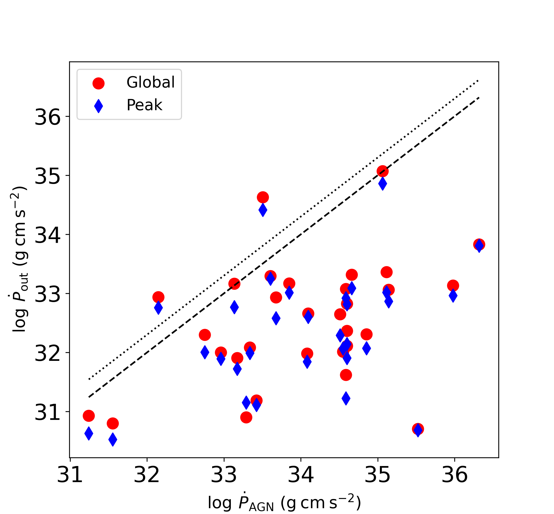
Figure 9: Momentum flux of the ionised outflows versus the AGN photon momentum flux for our sample. Red circles represent estimates obtained by assuming a spherical shell geometry and blue diamonds represent peak estimates from radial profiles. The dotted and dashed lines correspond to constant ratios of 2:1 and 1:1, respectively,useful to investigate the origin of the outflows.

In luminous quasars, the gas emission is usually dominated by outflowing gas (e.g. Kakkad et al., 2020; Vayner et al., 2021). Although ionised outflows are also frequently reported in lower luminosity AGN, a significant fraction of line emission in the inner kpc arises from gas with motions dominated by the gravitational potential of the galaxy (e.g. Davies et al., 2007; Schönell et al., 2019; Ruschel-Dutra et al., 2021; Fonseca-Faria et al., 2021; Bianchin et al., 2022). We find that 79 per cent of our sample present ionised outflows. Recently, Ruschel-Dutra et al. (2021) found outflows in 70 per cent of their sample composed of 30 AGN at $z\leq 0.02$ using optical Gemini GMOS-IFU observations, while Kakkad et al. (2022) studied ionised outflows in a sample of 22 X-ray selected AGN at $z\leq 0.1$ observed with the MUSE instrument at the VLT.

We find that the ionised outflows correspond to a median of 15 per cent of the mass of ionised gas in our sample. As shown in Table 2 and Fig. 7, our sample spans a wide range in fraction of gas in the outflow relative to the total gas mass, which is consistent with previous observations (e.g. Müller-Sánchez et al., 2011; Riffel et al., 2013b, 2020; Riffel, 2021; May et al., 2018; Bianchin et al., 2022). As shown in Fig. 7, there is a positive trend between the fraction of the gas in the outflow in ionised and molecular gas phases (middle panel), but there is no clear relation bewteen the masses of the gas in the outflow in both phases with the luminosity (right panel).

The fraction of objects with hot molecular outflows in our sample is 76 per cent. The contribution of hot molecular outflows to the total mass of hot molecular gas in the inner region of the observed galaxies is 13 per cent, while if we consider only galaxies with outflows, this contribution slightly increases to 15 per cent. This is consistent with previous observations of nearby active galaxies, which indicate that the hot molecular hydrogen in the inner kpc of nearby AGN hosts is more restricted to the galaxy disc, while the ionised gas usually presents an ouflowing component traced by gas that extends to higher latitudes above the disc (e.g. Riffel et al., 2015; Riffel et al., 2018b, 2021b; Ramos Almeida et al., 2017; Storchi-Bergmann & Schnorr-Müller, 2019; Speranza et al., 2022).

We can compare the properties of the outflows observed in both, hot molecular and ionised gas, phases. Wind scaling relations suggest that the molecular gas phases are relatively more important in lower luminosity objects, but similar to the ionised gas phase in higher luminosity AGN, as indicated by the higher slopes of the correlations of winds properties with the AGN bolometric luminosity observed in ionised gas, relative to those seen in cold molecular gas (Fiore et al., 2017). As shown in Fig. 7, we do not find a clear relation between the ratio of the gas masses of ionised and hot molecular gas with the luminosity. In addition, simulations aimed at investigating outflow properties as a function of radius for different gas phases, indicate that the molecular phase of the outflow is generated from the cooling of the gas trapped into the outflow, and so one would expect that the molecular phase is more important at larger radii, relative to the ionised phase (e.g. Ferrara & Scannapieco, 2016; Costa et al., 2018; Richings & Faucher-Giguère, 2018; Richings et al., 2021). As shown in the bottom panel of Fig. 5, we do not find a clear relation between the mass-outflow rates in ionised and hot molecular gas with the distance from the centre. A possible explanation for the absence of relations between the relative outflow properties in both phases with the luminosity and radius, is that the hot molecular gas phase observed via the H₂ emission lines represents only the heated surface of a much larger colder molecular gas reservoir (Dale et al., 2005; Mazzalay et al., 2013), considered in the simulations.

The mass-outflow rates and kinetic powers of the outflows estimated for our sample are in agreement with previous measurements for AGN of similar luminosity. However, as can be seen in Fig. 8, the scatters of the relations of $\log\>\dot{M}_{\rm out}$ versus $\log L_{\rm bol}$ and $\log\>\dot{E}_{\rm out}$ versus $\log L_{\rm bol}$ are high, if we consider all measurements available in the literature and used for comparison here. The density of the outflow is a function of the radius, as well as the ionised gas density at a given radius is a function of the AGN luminosity (Davies et al., 2020; Revalski et al., 2022), and thus the use of a fixed density value to estimate the mass-outflow rate may reduce the scatter of the correlation between $\log\>\dot{M}_{\rm out}$ and $\log L_{\rm bol}$. In the luminosity range of our sample, the mass-outflow rates in ionised gas cover four orders of magnitude, while the kinetic powers spans three orders of magnitude. The wide ranges of values observed for $\log\>\dot{M}_{\rm out}$ and $\log\>\dot{E}_{\rm out}$ are in good agreement with previous works and are partially due to the assumptions made to calculate the outflow properties by distinct works, which include assumptions on the electron density estimates, geometry, and velocity of the outflows (see Davies et al., 2020, for a detailed discussion). An important caveat is that outflow rates are defined as the amount of material passing through a common radius, so they may be estimated globally for the entire outflow, or outflow rates measured from individual spaxels, may be added azimuthally to produce radial outflow rate profiles (see Figure 5 and Revalski et al., 2021). However, outflow rates cannot be added radially. These instantaneous outflow rates are directly related to the spatial resolution of the data, such that higher spatial sampling yields larger instantaneous rates, because they account for material passing through multiple boundaries for a fixed evacuation time (Veilleux et al., 2017; Kakkad et al., 2022). This can explain why mass outflow rates and kinetic powers estimated by radially summing the individual spaxels are systematically larger by up to two orders of magnitude as compared to the global and radial estimates (e.g. Kakkad et al., 2022)

We can compare the kinetic coupling efficiencies ($\dot{E}_{K}/L_{\rm bol}$) for observed ionised outflows in our sample with theoretical predictions. For AGN feedback to become efficient in suppressing star formation, the models require a minimum coupling efficiency ($\varepsilon_{f}$) in the range of 0.5–20 per cent (Di Matteo et al., 2005; Hopkins & Elvis, 2010; Dubois et al., 2014; Schaye et al., 2015; Weinberger et al., 2017). However, as discussed in Harrison et al. (2018), it is unlikely that all the injected energy becomes kinetic power in the outflow and a direct comparison between observed $\dot{E}_{K}/L_{\rm bol}$ and predicted $\varepsilon_{f}$ is not straightforward. Indeed, recent numerical simulations indicate that the kinetic energy of the outflows represents less than 20 per cent of the total emitted outflow energy (Richings & Faucher-Giguère, 2018).

With the above caveat in mind, we estimate the kinetic coupling efficiencies for the ionised gas in our sample. We find that none object in our sample present outflows with kinetic powers corresponding to more than 0.5 per cent of the AGN bolometric luminosity. The median value of the kinetic coupling efficiency using the global kinetic power of the ionised outflows is $\dot{E}_{K}/L_{\rm bol}\approx 1.8\times 10^{-3}$. The kinetic powers of the hot molecular outflows are about 2 orders of magnitude lower than those of the ionised gas, and thus they are also not powerful enough to suppress star formation in the galaxies. However, besides the fact that $\dot{E}_{K}/L_{\rm bol}<\varepsilon_{f}$ mentioned above, the outflows in AGN are seen in multiple gas phases and the kinetic power of dense cold molecular outflows are expected to be larger. Thus, even if the ionised outflows seen here are not powerful enough to suppress star formation in the host galaxies, we cannot discard AGN feedback as an important mechanism in shaping the evolution of the galaxies in our sample.

In order to investigate the physical mechanism that drives the outflows observed in our sample, we compute the momentum flux of the outflow by $\dot{P}_{\rm out}=\dot{M}\times v_{\rm out}$, where $v_{\rm out}$ is the velocity of the outflow. In Figure 9, we present a plot of $\dot{P}_{\rm out}$ versus the photon momentum flux ($\dot{P}_{\rm AGN}=L_{\rm AGN}/c$, where $L_{\rm AGN}$ is the AGN bolometric luminosity), which can yield insights into the origin of winds (Murray et al., 2005; Thompson et al., 2015; Costa et al., 2018; Veilleux et al., 2020; Vayner et al., 2021). To estimate $\dot{P}_{\rm out}$, we use the same definition for the velocity of the outflow previously used to calculate the mass-outflow rates. The dotted and dashed lines show a 2:1 and 1:1 constant relations respectively, that can be used to investigate the the driving mechanism of the outflows. Theoretical studies suggest that $\dot{P}_{\rm out}\gtrsim 2\dot{P}_{\rm AGN}$ on scales $\lesssim$1 kpc are due to radiation pressure driven winds in a high-density, optically thick environment, where far-infrared photons are scattered multiple times (Thompson et al., 2015; Costa et al., 2018). Values of $\dot{P}_{\rm out}\lesssim 1\dot{P}_{\rm AGN}$ are usually attributed to radiation-pressure driven winds in low density environments or shocked AGN winds (Faucher-Giguère & Quataert, 2012). Most objects in our sample are below the 1:1 line in Fig. 9, indicating that the winds are driven by radiation-pressure in low-density environment, with possible contribution from shocks as suggested also in our previous studies (e.g. Riffel et al., 2021b; Riffel et al., 2021a).

6 Conclusions

We have studied the molecular and ionised gas kinematics of the inner 0.04–2 kpc of a sample of 33 AGN hosts with $0.001\lesssim z\lesssim 0.056$ and hard X-ray luminosities of $41\lesssim\log L_{\rm X}/({\rm erg\,s^{-1}})\lesssim 45$. The K-band observations were performed with the Gemini NIFS instrument, with a field of view covering from the inner 75$\times$75 pc² to 3.6$\times$3.6 kpc² at spatial resolutions of 6 to 250 pc and velocity resolution of $\sigma_{\rm inst}\sim$20 km s^-1. We use the $W_{\rm 80}$, $V_{\rm peak}$ and $V_{\rm cen}$ parameters for the H${}_{2}\>2.1218\,\mu$m and Br$\gamma$ emission lines to identify regions where the gas motions are dominated by kinematic disturbances due to the AGN and regions where the gas motions are due the gravitational potential of galaxies. Our main conclusions are:

• We identify ionised gas kinematically disturbed regions (KDRs) in 31 galaxies (94 per cent) of our sample, while 25 objects (76 per cent) present KDRs in molecular gas.

• We attribute the KDR as being produced by AGN outflows and estimate their mass-outflow rates and kinetic powers in two ways: (i) by assuming an spherical geometry, resulting in global outflow properties and (ii) adopting the peak outflow properties, derived from their radial profiles.

• The masses of the outflowing gas are in the ranges 10²–10⁷ M_⊙ and 10⁰–10⁴ M_⊙ for the ionised and hot molecular gas, respectively. These values correspond to median fractions of the gas in the outflow relative to the total amount of gas of about 15 per cent for both ionised and hot molecular gas (within a typical covered region of a few 100 pc radius at the galaxies).

• The mass-outflow rates in ionised gas are in the range 10^-3–10¹ M_⊙ yr^-1. The kinetic powers of the ionised outflows are in the range $\sim$10³⁷–10⁴³ erg s^-1, being smaller than 0.5 per cent of the AGN bolometric luminosity for most objects, with a median kinetic coupling efficiency in our sample is $\dot{E}_{K}/L_{\rm bol}\approx 1.8\times 10^{-3}$. The estimated mass-outflow rates and kinetic powers of the outflows are consistent with previous estimates for objects in the same luminosity range, but a large scatter of the wind scaling relations is seen in the lower luminosity range.

• The mass-outflow rates in molecular gas range from 10^-5 to 10^-2 M_⊙ yr^-1, and the kinetic power of the outflows are in the range 10³⁵–10³⁹ erg s^-1. Both mass outflow rates and powers present positive correlations with the AGN bolometric luminosity.

• The momentum flux of the ionised outflows are lower than the photon momentum flux of the accretion disc in most objects, indicating that the observed outflows are consistent with radiation-pressure driven winds in low density environments including possible contribution of shocked AGN winds.

In summary, our results support the presence of kinematic disturbances produced by the AGN in most sources, with a higher impact in the galaxy produced by the ionised gas outflows as compared to that of the hot molecular gas. This can be attributed mostly to the small mass in this latter gas phase, but its kinematics is also dominated by lower velocities than observed in the ionised gas. Observations in cold molecular gas should be made to investigate the presence of outflows in this gas phase.

Data availability

The data used in this paper is available in the Gemini Science Archive at https://archive.gemini.edu/searchform. Processed datacubes used will be shared on reasonable request to the corresponding author.

Supplementary Materials

Appendix A Results for individual galaxies

In figures 10 to 42, we present the maps, distributions and stacked profiles for all galaxies in our sample.

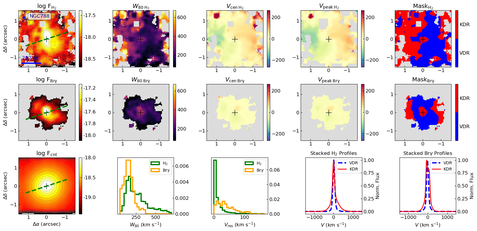
Figure 10: Results for NGC788. The first row shows the results for the H${}_{2}\>2.1218\,\mu$m  and second row show results for the the Br$\gamma$ emission line. From left to right: emission line flux distribution, $W_{\rm 80}$, $V_{\rm cen}$, $V_{\rm peak}$, and a “kinematic map” identifying the kinematically disturbed region (KDR) in red and the virially-dominated region (VDR) in blue. The colour bars show fluxes in erg s^-1 cm^-2 spaxel^-1 and velocities in km s^-1. The grey areas identify locations where the emission-line amplitude is below 3 times the continuum noise amplitude (3$\sigma$). The bottom rows show a K-band continuum image in erg s^-1 cm^-2 Å^-1 spaxel^-1, the density distributions of $W_{\rm 80}$ and $V_{\rm res}=|V_{\rm cen}-V_{\rm peak}|$ and stacked profiles of the H₂ and Br$\gamma$ emission lines from the VDR and KDR. Stacked profiles for the KDR are presented only if it corresponds to at least 10 per cent of the spaxels with detected emission. The green dashed lines in the leftmost panels show the orientation of the major axis of the large-scale disk, as presented in Riffel et al. (2021b). In all maps, North is up and East is to the left.

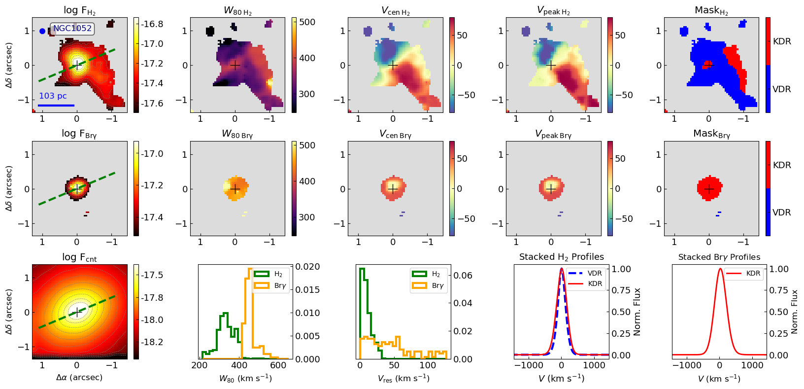
Figure 11: Same as Fig. 10, but for NGC 1052.

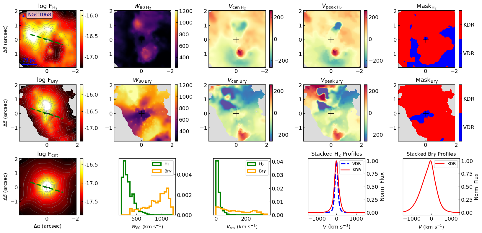
Figure 12: Same as Fig. 10, but for NGC 1068.

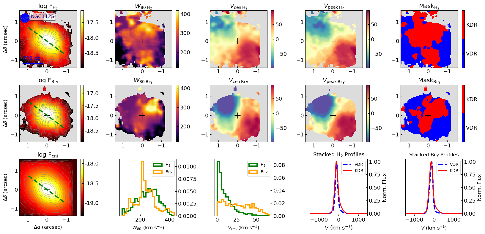
Figure 13: Same as Fig. 10, but for NGC 1125.

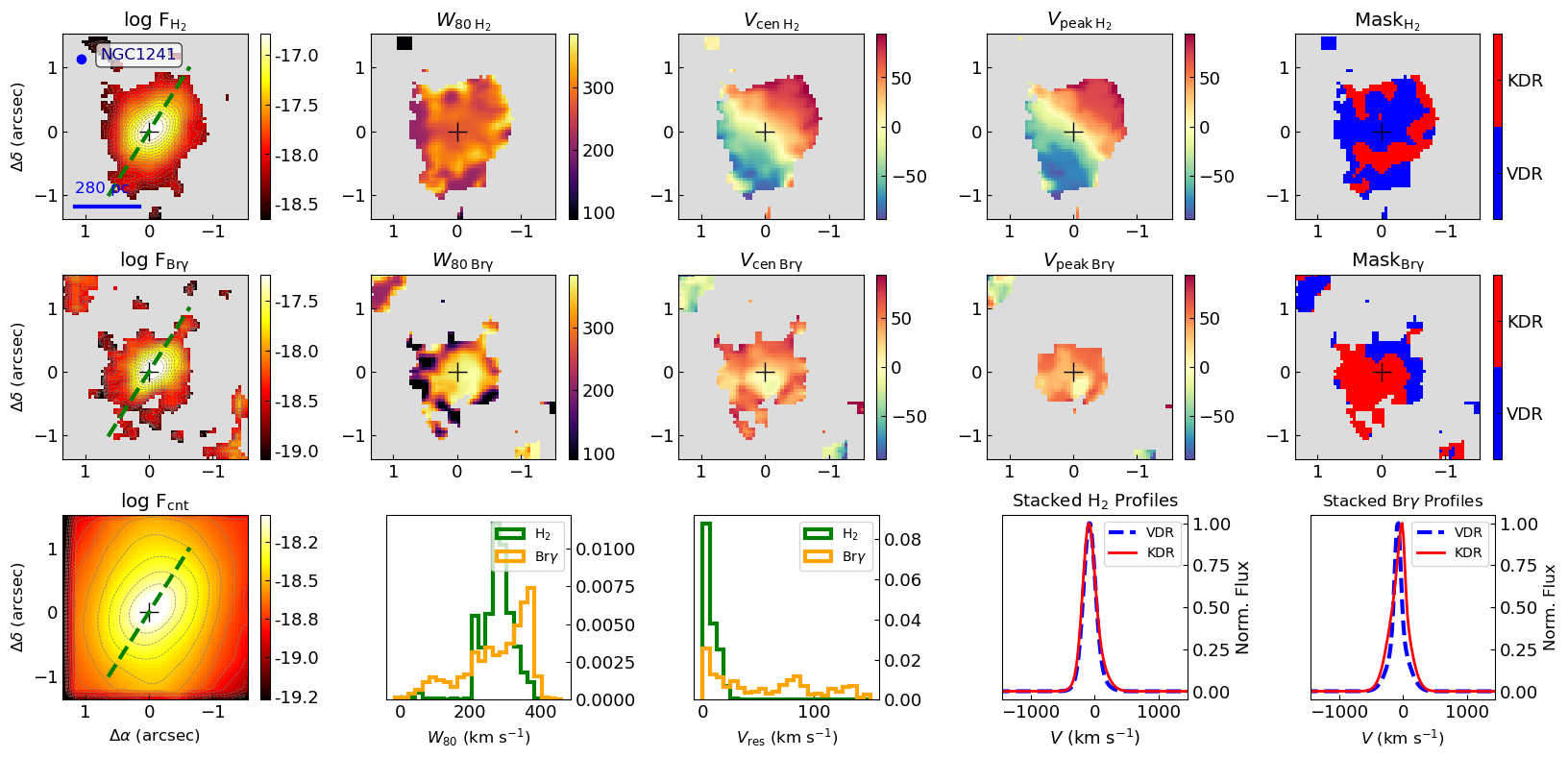
Figure 14: Same as Fig. 10, but for NGC 1241.

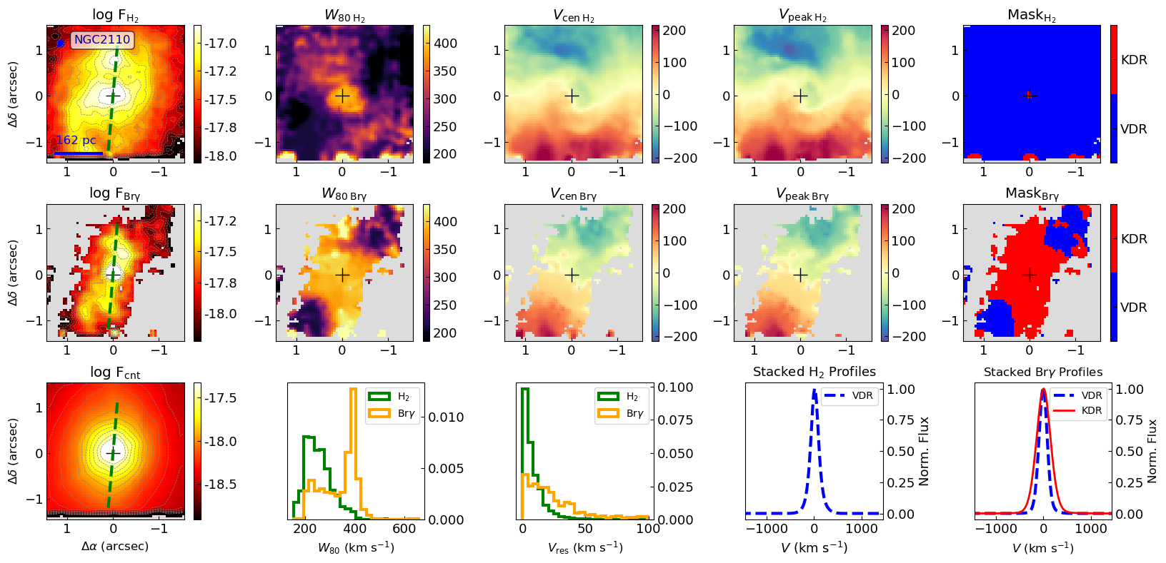
Figure 15: Same as Fig. 10, but for NGC 2110.

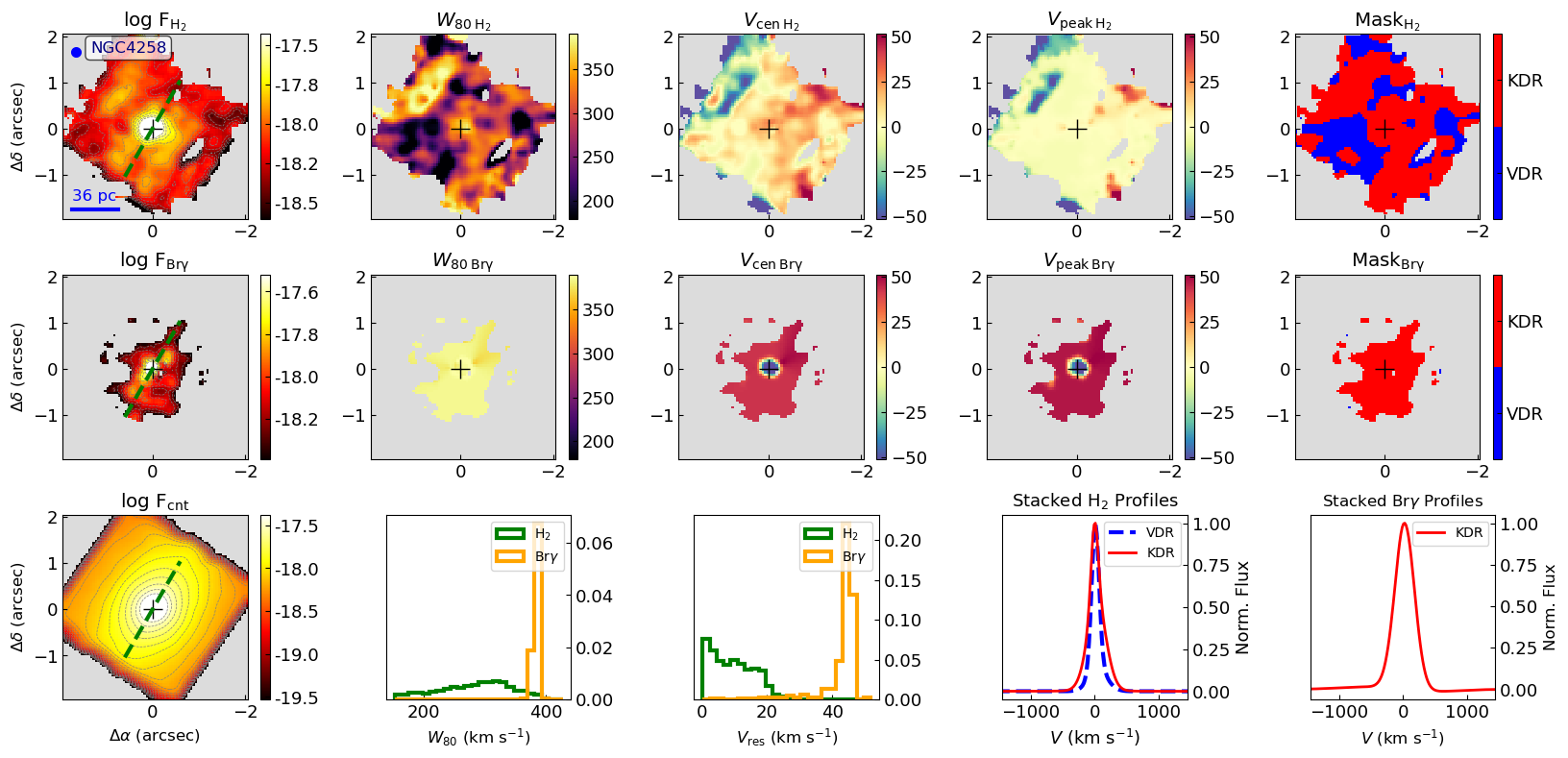
Figure 16: Same as Fig. 10, but for NGC 4258.

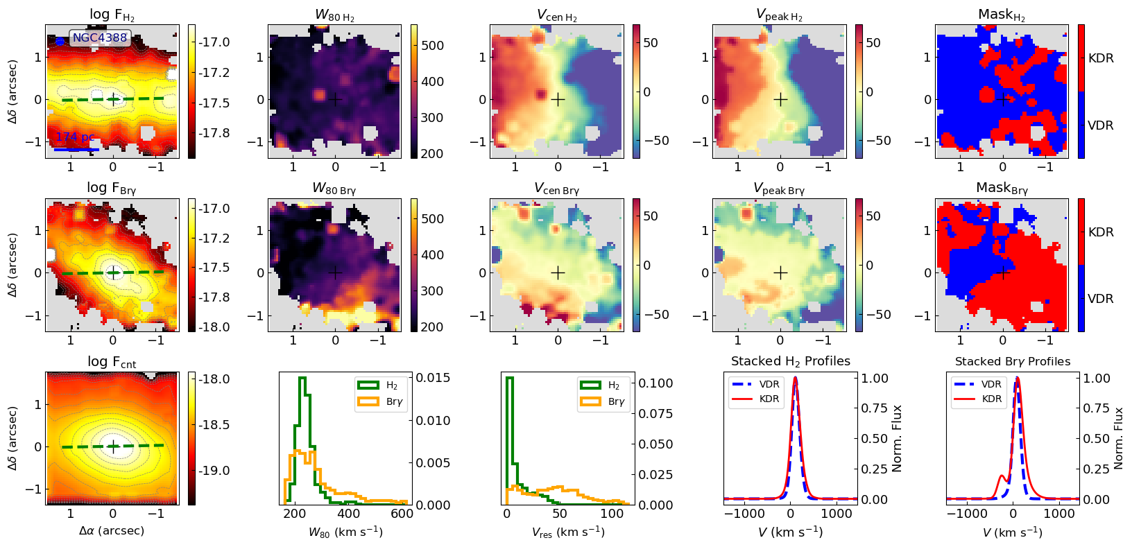
Figure 17: Same as Fig. 10, but for NGC 4388.

Figure 18: Same as Fig. 10, but for NGC 5506.

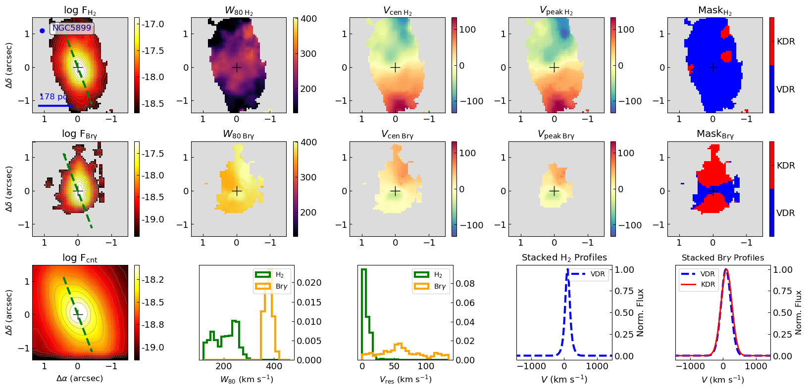
Figure 19: Same as Fig. 10, but for NGC 5899.

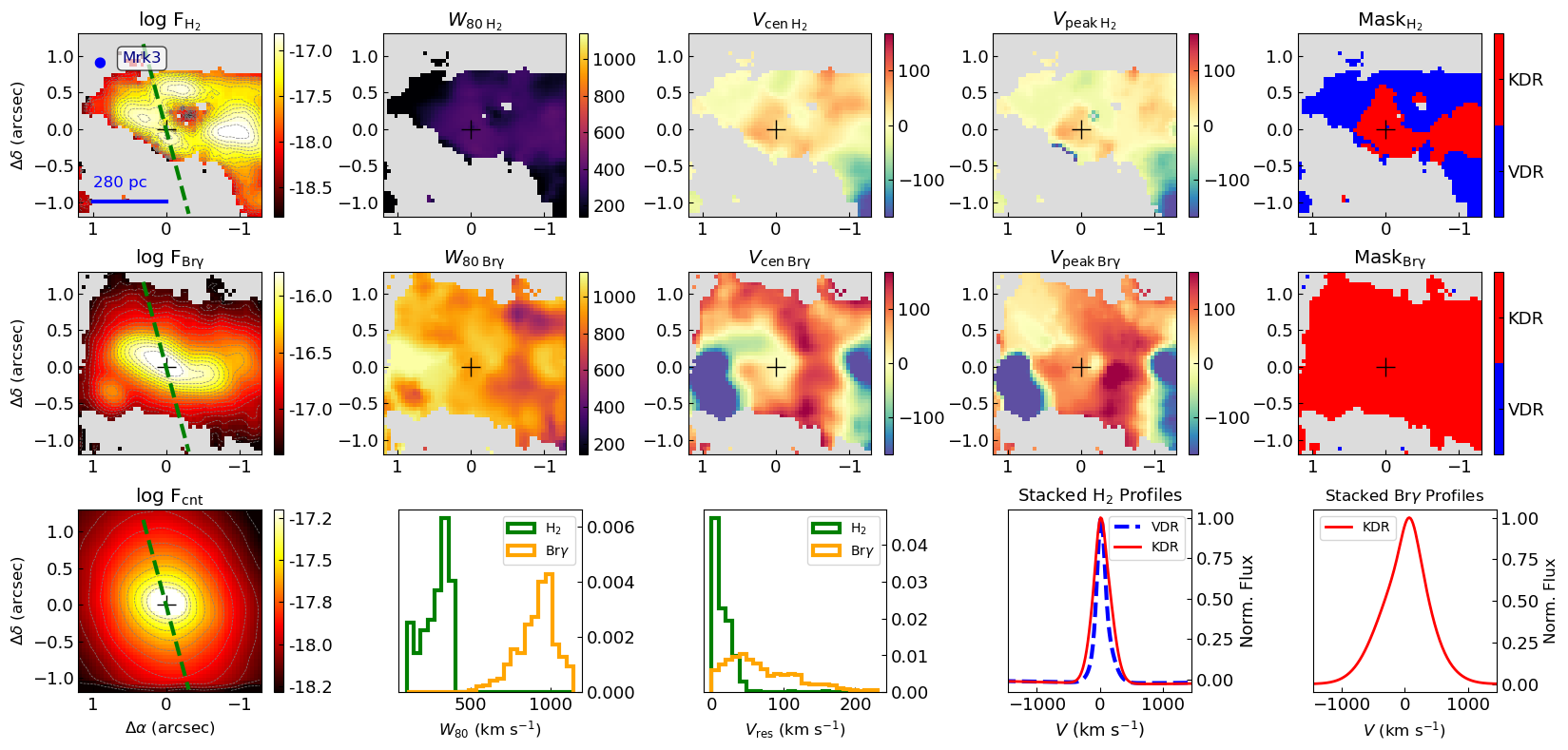
Figure 20: Same as Fig. 10, but for Mrk 3.

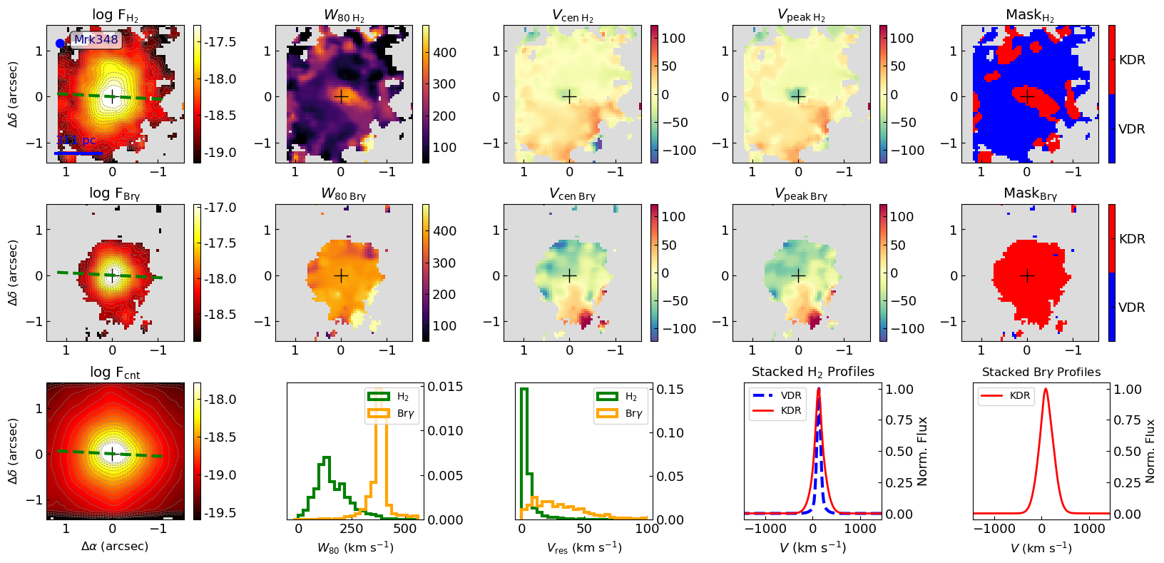
Figure 21: Same as Fig. 10, but for Mrk 348.

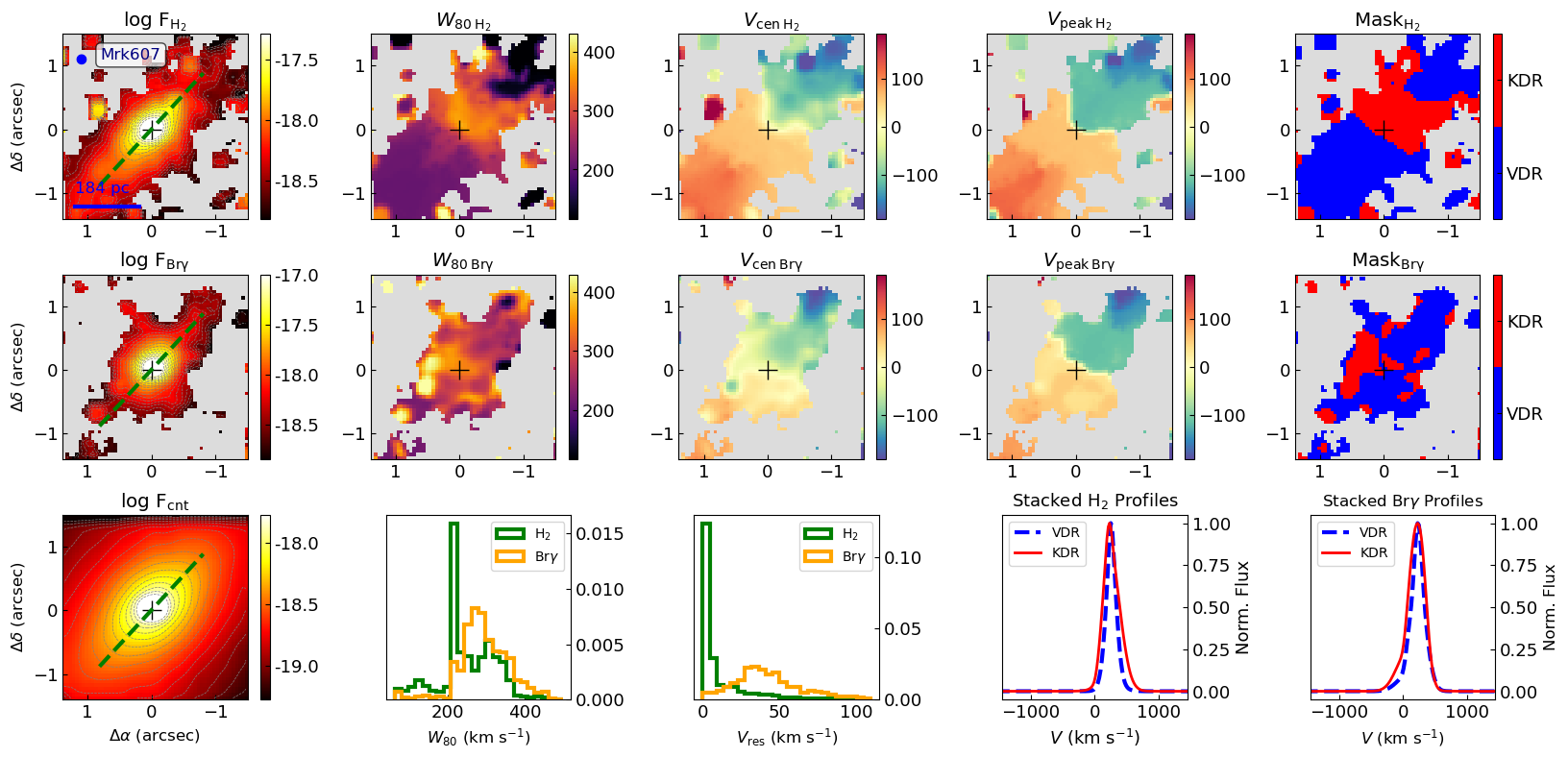
Figure 22: Same as Fig. 10, but for Mrk 607.

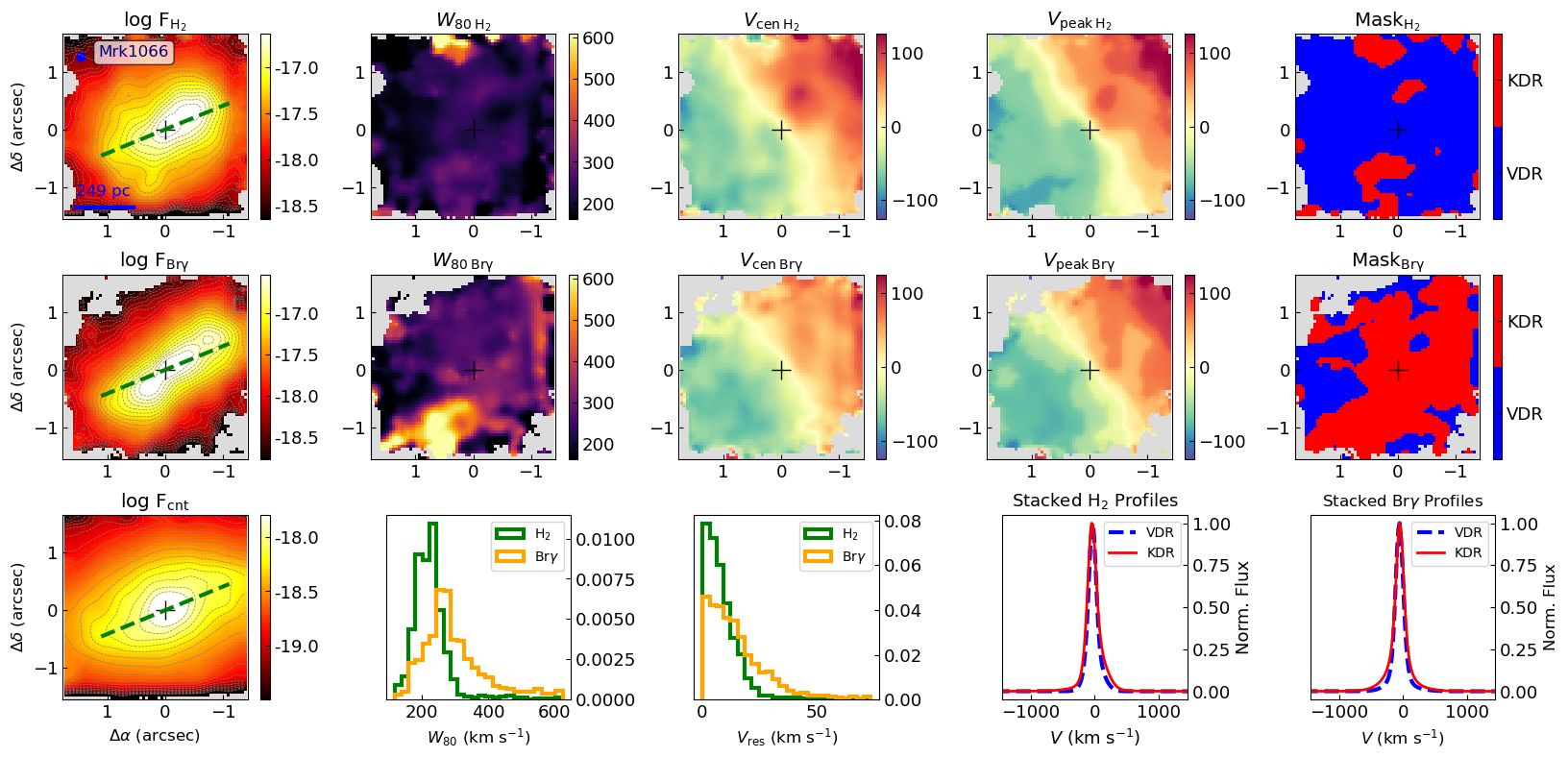
Figure 23: Same as Fig. 10, but for Mrk 1066.

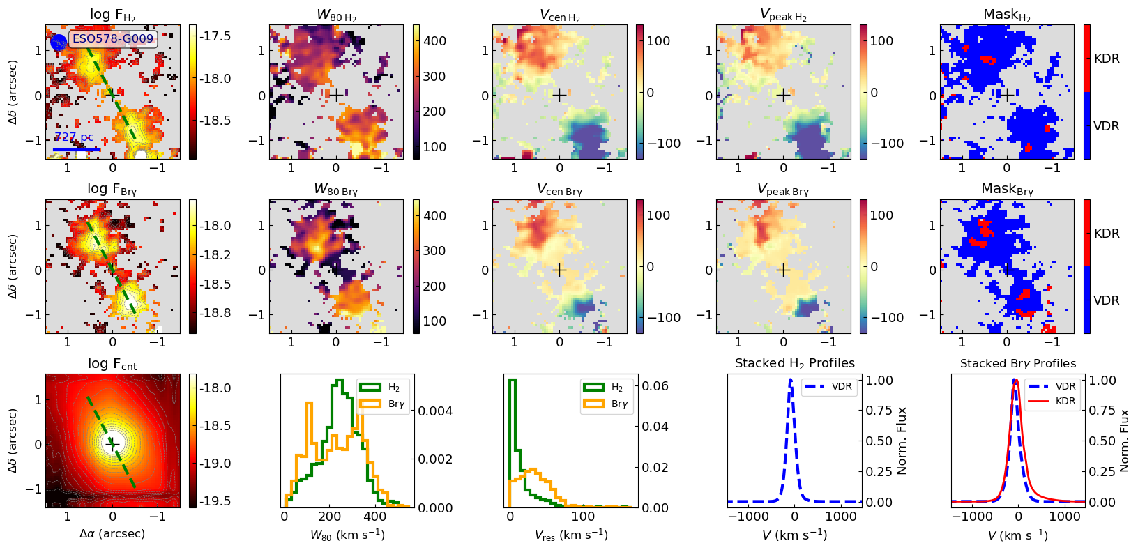
Figure 24: Same as Fig. 10, but for ESO 578-G009.

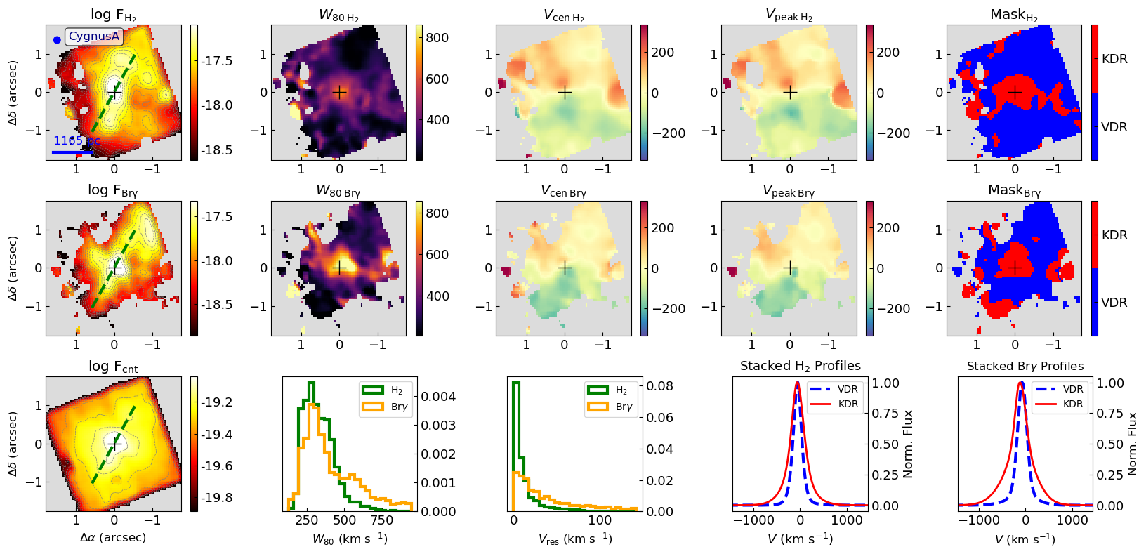
Figure 25: Same as Fig. 10, but for Cygnus A.

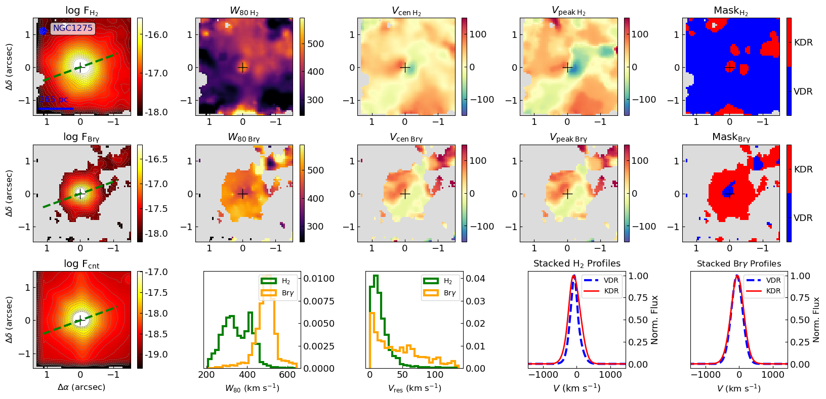
Figure 26: Same as Fig. 10, but for NGC 1275.

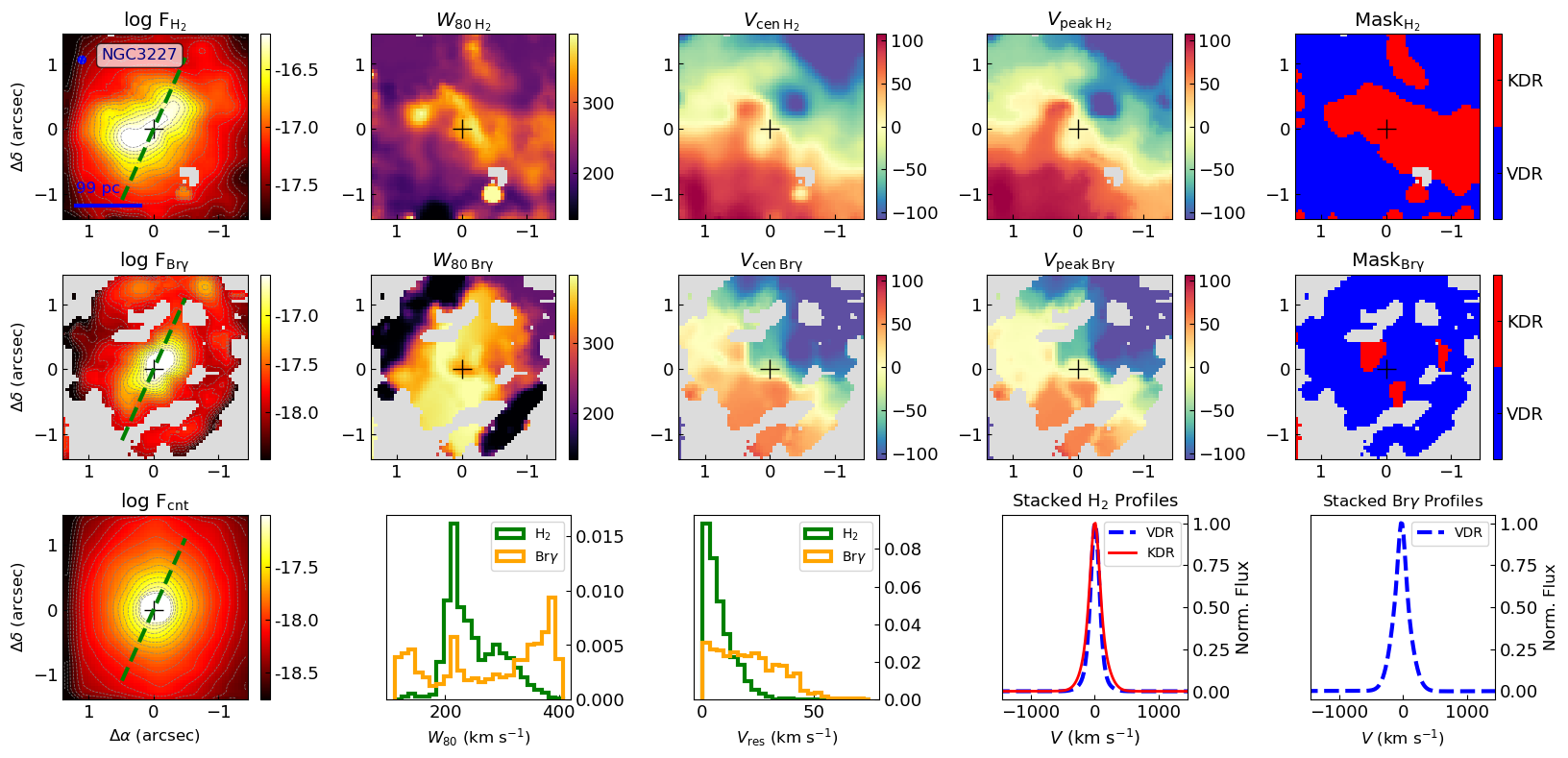
Figure 27: Same as Fig. 10, but for NGC 3227.

Figure 28: Same as Fig. 10, but for NGC 3516.

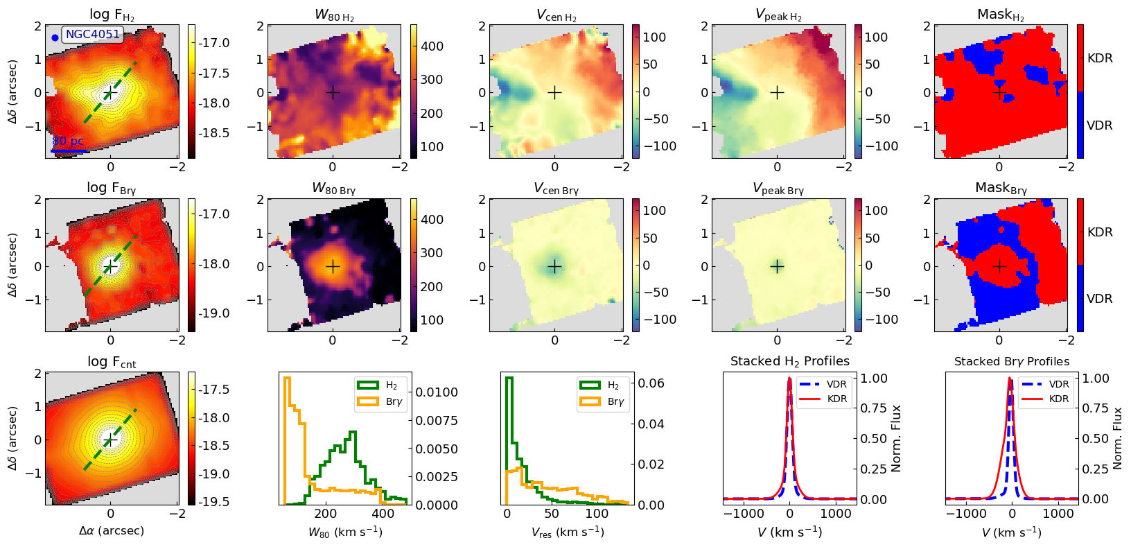
Figure 29: Same as Fig. 10, but for NGC 4051.

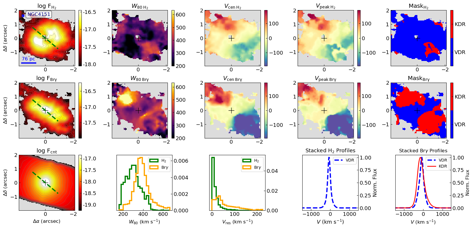
Figure 30: Same as Fig. 10, but for NGC 4151.

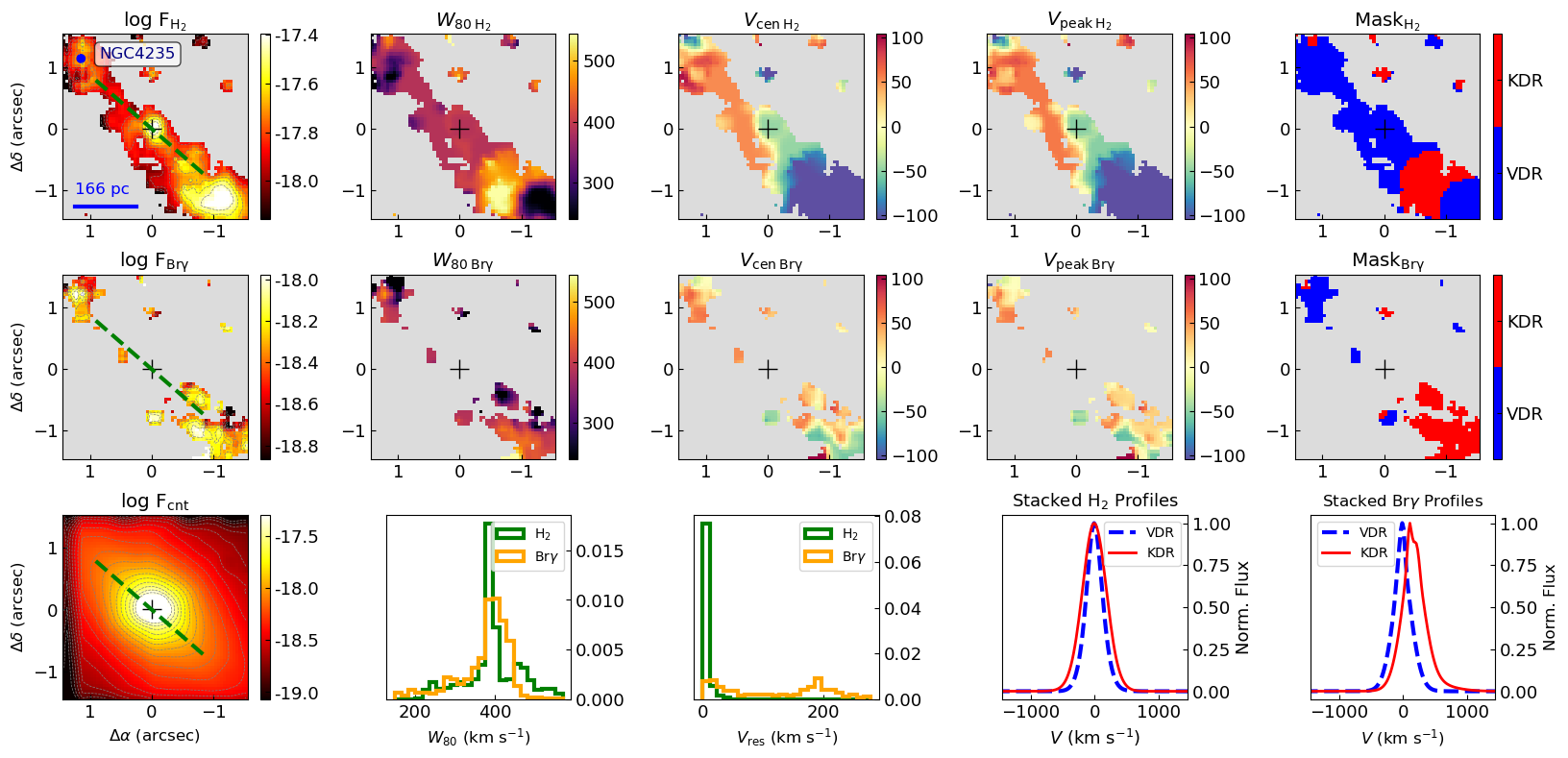
Figure 31: Same as Fig. 10, but for NGC 4325.

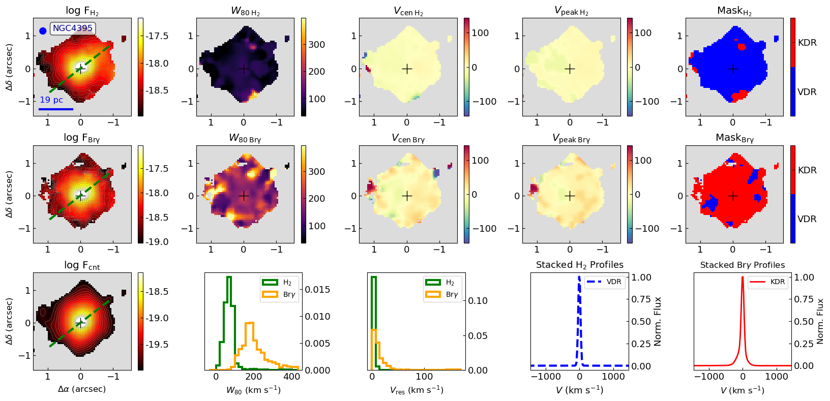
Figure 32: Same as Fig. 10, but for NGC 4395.

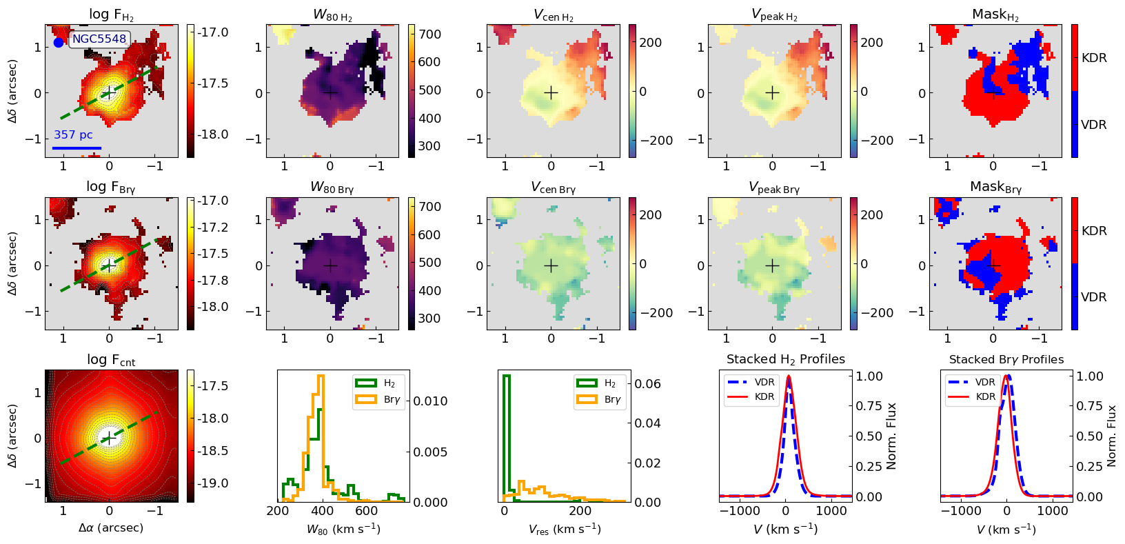
Figure 33: Same as Fig. 10, but for NGC 5548.

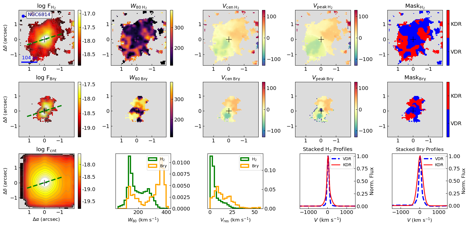
Figure 34: Same as Fig. 10, but for NGC 6814.

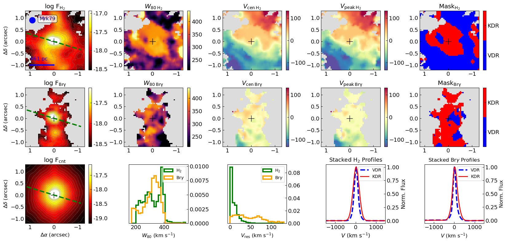
Figure 35: Same as Fig. 10, but for Mrk 79.

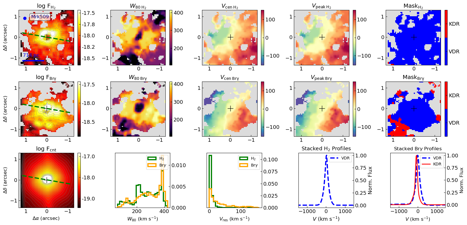
Figure 36: Same as Fig. 10, but for Mrk 509.

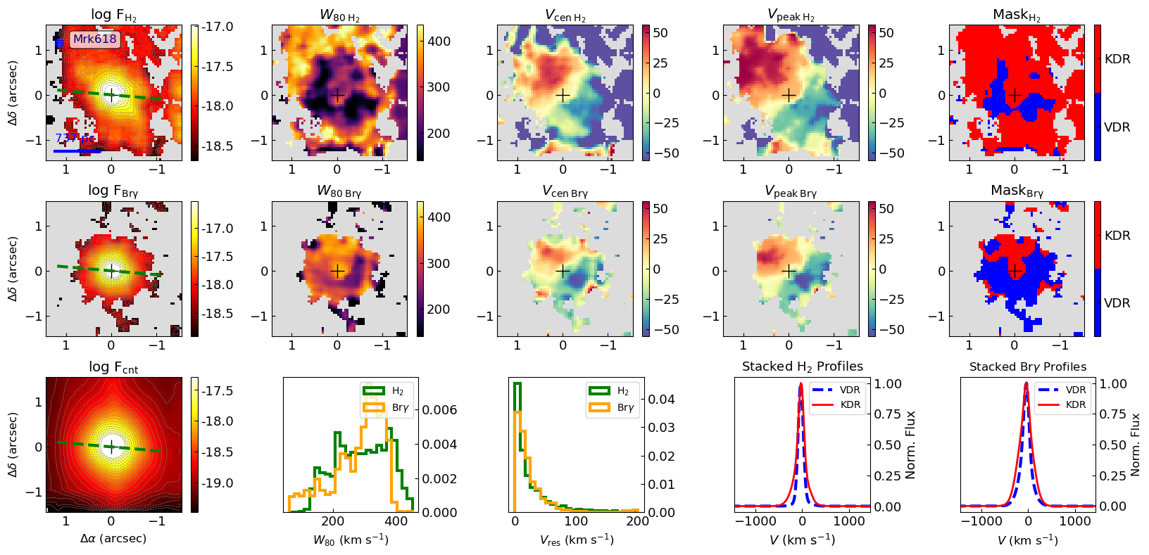
Figure 37: Same as Fig. 10, but for Mrk 618.

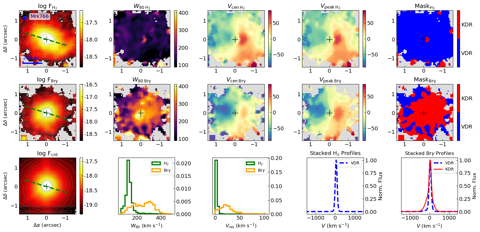
Figure 38: Same as Fig. 10, but for Mrk 766.

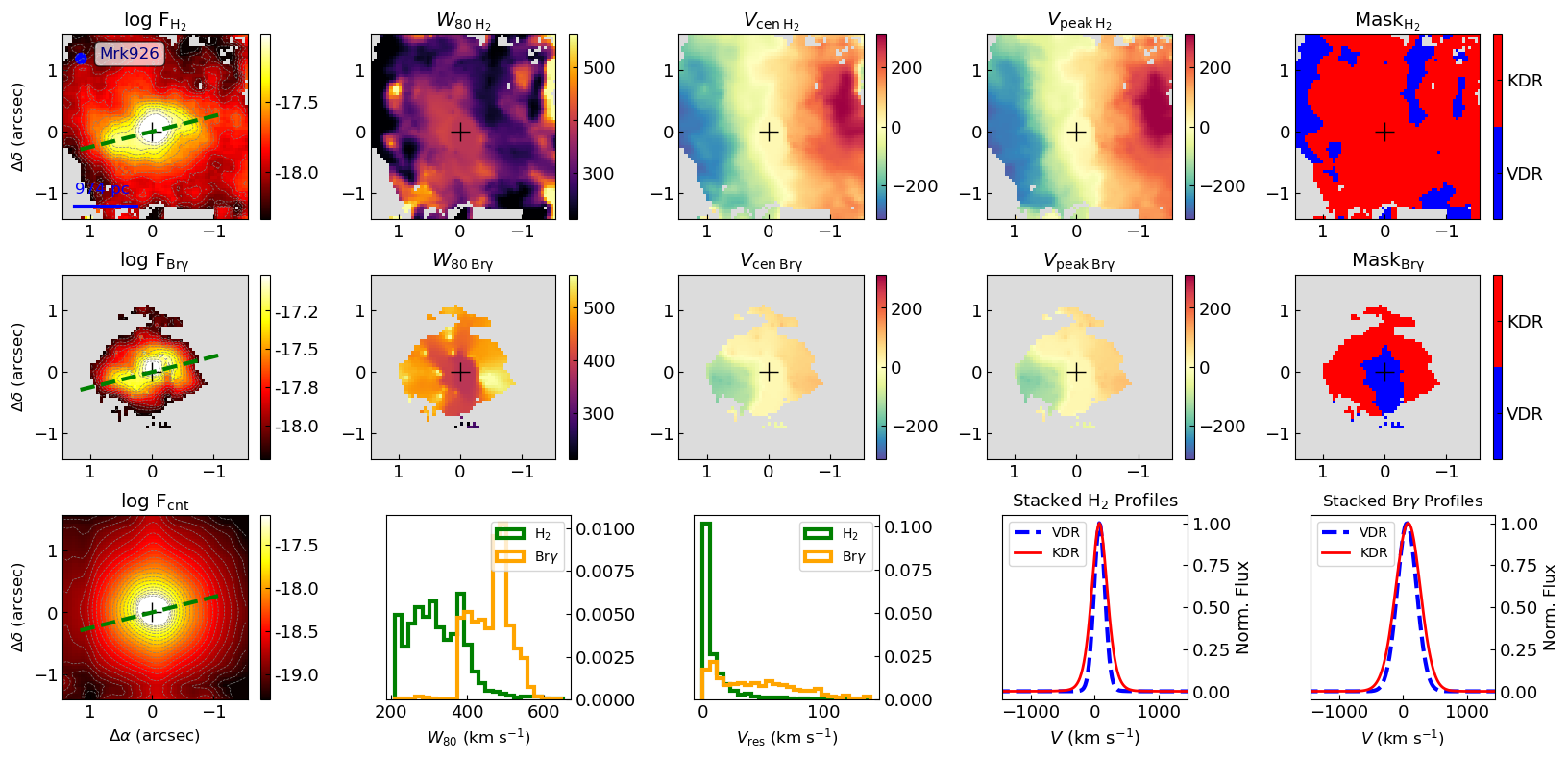
Figure 39: Same as Fig. 10, but for Mrk 926.

Figure 40: Same as Fig. 10, but for Mrk 1044.

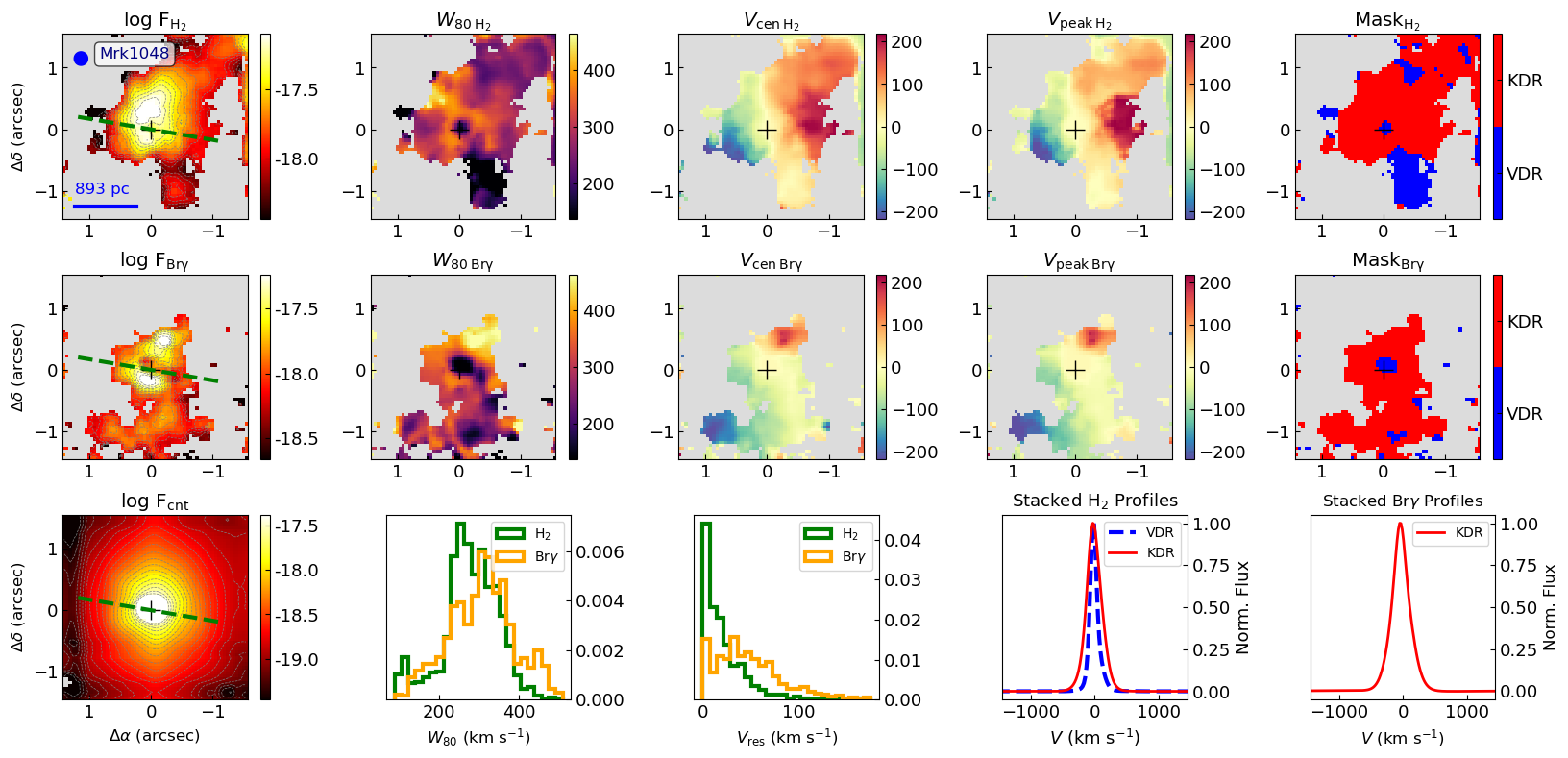
Figure 41: Same as Fig. 10, but for Mrk 1048.

Figure 42: Same as Fig. 10, but for MCG+08-11-011.

References

- Avery et al. (2021) Avery C. R., et al., 2021, MNRAS, 503, 5134
- Barbosa et al. (2014) Barbosa F. K. B., Storchi-Bergmann T., McGregor P., Vale T. B., Rogemar Riffel A., 2014, MNRAS, 445, 2353
- Baron & Netzer (2019) Baron D., Netzer H., 2019, MNRAS, 486, 4290
- Bentz et al. (2019) Bentz M. C., Ferrarese L., Onken C. A., Peterson B. M., Valluri M., 2019, ApJ, 885, 161
- Bianchin et al. (2022) Bianchin M., et al., 2022, MNRAS, 510, 639
- Brum et al. (2017) Brum C., Riffel R. A., Storchi-Bergmann T., Robinson A., Schnorr Müller A., Lena D., 2017, MNRAS, 469, 3405
- Burtscher et al. (2015) Burtscher L., et al., 2015, A&A, 578, A47
- Burtscher et al. (2021) Burtscher L., et al., 2021, A&A, 654, A132
- Caglar et al. (2020) Caglar T., et al., 2020, A&A, 634, A114
- Cappellari (2017) Cappellari M., 2017, MNRAS, 466, 798
- Cappellari & Emsellem (2004) Cappellari M., Emsellem E., 2004, PASP, 116, 138
- Ciotti et al. (2010) Ciotti L., Ostriker J. P., Proga D., 2010, ApJ, 717, 708
- Costa et al. (2018) Costa T., Rosdahl J., Sijacki D., Haehnelt M. G., 2018, MNRAS, 479, 2079
- Couto et al. (2020) Couto G. S., Storchi-Bergmann T., Siemiginowska A., Riffel R. A., Morganti R., 2020, MNRAS, 497, 5103
- Dale et al. (2005) Dale D. A., Sheth K., Helou G., Regan M. W., Hüttemeister S., 2005, AJ, 129, 2197
- Dall’Agnol de Oliveira et al. (2021) Dall’Agnol de Oliveira B., et al., 2021, MNRAS, 504, 3890
- Davies et al. (2007) Davies R. I., Müller Sánchez F., Genzel R., Tacconi L. J., Hicks E. K. S., Friedrich S., Sternberg A., 2007, ApJ, 671, 1388
- Davies et al. (2020) Davies R., et al., 2020, MNRAS,
- Deconto-Machado et al. (2022) Deconto-Machado A., et al., 2022, arXiv e-prints, p. arXiv:2201.01690
- Di Matteo et al. (2005) Di Matteo T., Springel V., Hernquist L., 2005, Nature, 433, 604
- Diniz et al. (2015) Diniz M. R., Riffel R. A., Storchi-Bergmann T., Winge C., 2015, MNRAS, 453, 1727
- Diniz et al. (2017) Diniz M. R., Riffel R. A., Riffel R., Crenshaw D. M., Storchi-Bergmann T., Fischer T. C., Schmitt H. R., Kraemer S. B., 2017, MNRAS, 469, 3286
- Diniz et al. (2019) Diniz M. R., Riffel R. A., Storchi-Bergmann T., Riffel R., 2019, MNRAS, 487, 3958
- Dors et al. (2014) Dors O. L., Cardaci M. V., Hägele G. F., Krabbe Â. C., 2014, MNRAS, 443, 1291
- Dors et al. (2020) Dors O. L., Maiolino R., Cardaci M. V., Hägele G. F., Krabbe A. C., Pérez-Montero E., Armah M., 2020, MNRAS,
- Dubois et al. (2014) Dubois Y., et al., 2014, MNRAS, 444, 1453
- Elvis (2000) Elvis M., 2000, ApJ, 545, 63
- Faucher-Giguère & Quataert (2012) Faucher-Giguère C.-A., Quataert E., 2012, MNRAS, 425, 605
- Ferrara & Scannapieco (2016) Ferrara A., Scannapieco E., 2016, ApJ, 833, 46
- Ferrarese & Merritt (2000) Ferrarese L., Merritt D., 2000, ApJ, 539, L9
- Fiore et al. (2017) Fiore F., et al., 2017, A&A, 601, A143
- Fischer et al. (2018) Fischer T. C., et al., 2018, ApJ, 856, 102
- Fischer et al. (2019) Fischer T. C., et al., 2019, ApJ, 875, 102
- Fonseca-Faria et al. (2021) Fonseca-Faria M. A., Rodríguez-Ardila A., Contini M., Reynaldi V., 2021, MNRAS, 506, 3831
- Förster Schreiber et al. (2019) Förster Schreiber N. M., et al., 2019, ApJ, 875, 21
- Frank et al. (2002) Frank J., King A., Raine D. J., 2002, Accretion Power in Astrophysics: Third Edition
- Freitas et al. (2018) Freitas I. C., et al., 2018, MNRAS, 476, 2760
- Gebhardt et al. (2000) Gebhardt K., et al., 2000, ApJ, 539, L13
- Gültekin et al. (2009) Gültekin K., et al., 2009, ApJ, 698, 198
- Harrison (2017) Harrison C. M., 2017, Nature Astronomy, 1, 0165
- Harrison et al. (2018) Harrison C. M., Costa T., Tadhunter C. N., Flütsch A., Kakkad D., Perna M., Vietri G., 2018, Nature Astronomy, 2, 198
- Heckman & Kauffmann (2011) Heckman T. M., Kauffmann G., 2011, Science, 333, 182
- Hicks et al. (2013) Hicks E. K. S., Davies R. I., Maciejewski W., Emsellem E., Malkan M. A., Dumas G., Müller-Sánchez F., Rivers A., 2013, ApJ, 768, 107
- Hopkins & Elvis (2010) Hopkins P. F., Elvis M., 2010, MNRAS, 401, 7
- Ichikawa et al. (2017) Ichikawa K., Ricci C., Ueda Y., Matsuoka K., Toba Y., Kawamuro T., Trakhtenbrot B., Koss M. J., 2017, ApJ, 835, 74
- Ilha et al. (2016) Ilha G. d. S., Bianchin M., Riffel R. A., 2016, Ap&SS, 361, 178
- Ilha et al. (2019) Ilha G. S., et al., 2019, MNRAS, 484, 252
- Kakkad et al. (2018) Kakkad D., et al., 2018, A&A, 618, A6
- Kakkad et al. (2020) Kakkad D., et al., 2020, A&A, 642, A147
- Kakkad et al. (2022) Kakkad D., et al., 2022, MNRAS, 511, 2105
- Kormendy & Ho (2013) Kormendy J., Ho L. C., 2013, ARA&A, 51, 511
- Kovačević-Dojčinović et al. (2022) Kovačević-Dojčinović J., Dojčinović I., Lakićević M., Popović L. Č., 2022, A&A, 659, A130
- Lamperti et al. (2017) Lamperti I., et al., 2017, MNRAS, 467, 540
- Lamperti et al. (2021) Lamperti I., et al., 2021, A&A, 654, A90
- Liu et al. (2013) Liu G., Zakamska N. L., Greene J. E., Nesvadba N. P. H., Liu X., 2013, MNRAS, 436, 2576
- Luo et al. (2021) Luo R., et al., 2021, ApJ, 908, 221
- Lutz et al. (2020) Lutz D., et al., 2020, A&A, 633, A134
- Magorrian et al. (1998) Magorrian J., et al., 1998, AJ, 115, 2285
- Mallmann et al. (2018) Mallmann N. D., et al., 2018, MNRAS, 478, 5491
- May et al. (2018) May D., Rodríguez-Ardila A., Prieto M. A., Fernández-Ontiveros J. A., Diaz Y., Mazzalay X., 2018, MNRAS, 481, L105
- Mazzalay et al. (2013) Mazzalay X., et al., 2013, MNRAS, 428, 2389
- Mazzalay et al. (2014) Mazzalay X., et al., 2014, MNRAS, 438, 2036
- McElroy et al. (2015) McElroy R., Croom S. M., Pracy M., Sharp R., Ho I. T., Medling A. M., 2015, MNRAS, 446, 2186
- McGregor et al. (2003) McGregor P. J., et al., 2003, Gemini near-infrared integral field spectrograph (NIFS). Proceedings of the SPIE, pp 1581–1591, doi:10.1117/12.459448
- Mingozzi et al. (2019) Mingozzi M., et al., 2019, A&A, 622, A146
- Müller-Sánchez et al. (2011) Müller-Sánchez F., Prieto M. A., Hicks E. K. S., Vives-Arias H., Davies R. I., Malkan M., Tacconi L. J., Genzel R., 2011, ApJ, 739, 69
- Müller-Sánchez et al. (2018) Müller-Sánchez F., Nevin R., Comerford J. M., Davies R. I., Privon G. C., Treister E., 2018, Nature, 556, 345
- Murray et al. (2005) Murray N., Quataert E., Thompson T. A., 2005, ApJ, 618, 569
- Oh et al. (2018) Oh K., et al., 2018, ApJS, 235, 4
- Osterbrock & Ferland (2006) Osterbrock D. E., Ferland G. J., 2006, Astrophysics of gaseous nebulae and active galactic nuclei. University Science Books
- Penny et al. (2018) Penny S. J., et al., 2018, MNRAS, 476, 979
- Perna et al. (2017) Perna M., Lanzuisi G., Brusa M., Cresci G., Mignoli M., 2017, A&A, 606, A96
- Perrotta et al. (2019) Perrotta S., Hamann F., Zakamska N. L., Alexandroff R. M., Rupke D., Wylezalek D., 2019, MNRAS, 488, 4126
- Ramos Almeida et al. (2017) Ramos Almeida C., Piqueras López J., Villar-Martín M., Bessiere P. S., 2017, MNRAS, 470, 964
- Ramos Almeida et al. (2019) Ramos Almeida C., Acosta-Pulido J. A., Tadhunter C. N., González-Fernández C., Cicone C., Fernández-Torreiro M., 2019, MNRAS, 487, L18
- Reid et al. (2019) Reid M. J., Pesce D. W., Riess A. G., 2019, ApJ, 886, L27
- Revalski et al. (2021) Revalski M., et al., 2021, ApJ, 910, 139
- Revalski et al. (2022) Revalski M., et al., 2022, arXiv e-prints, p. arXiv:2203.07387
- Ricci et al. (2017) Ricci C., et al., 2017, ApJS, 233, 17
- Richings & Faucher-Giguère (2018) Richings A. J., Faucher-Giguère C.-A., 2018, MNRAS, 478, 3100
- Richings et al. (2021) Richings A. J., Faucher-Giguère C.-A., Stern J., 2021, MNRAS, 503, 1568
- Riffel (2021) Riffel R. A., 2021, MNRAS, 506, 2950
- Riffel & Storchi-Bergmann (2011a) Riffel R. A., Storchi-Bergmann T., 2011a, MNRAS, 411, 469
- Riffel & Storchi-Bergmann (2011b) Riffel R. A., Storchi-Bergmann T., 2011b, MNRAS, 417, 2752
- Riffel et al. (2006) Riffel R., Rodríguez-Ardila A., Pastoriza M. G., 2006, A&A, 457, 61
- Riffel et al. (2009) Riffel R. A., Storchi-Bergmann T., Dors O. L., Winge C., 2009, MNRAS, 393, 783
- Riffel et al. (2010) Riffel R. A., Storchi-Bergmann T., Riffel R., Pastoriza M. G., 2010, ApJ, 713, 469
- Riffel et al. (2011) Riffel R., Riffel R. A., Ferrari F., Storchi-Bergmann T., 2011, MNRAS, 416, 493
- Riffel et al. (2013a) Riffel R. A., Storchi-Bergmann T., Winge C., 2013a, MNRAS, 430, 2249
- Riffel et al. (2013b) Riffel R. A., Storchi-Bergmann T., Winge C., 2013b, MNRAS, 430, 2249
- Riffel et al. (2014) Riffel R. A., Vale T. B., Storchi-Bergmann T., McGregor P. J., 2014, MNRAS, 442, 656
- Riffel et al. (2015) Riffel R. A., Storchi-Bergmann T., Riffel R., 2015, MNRAS, 451, 3587
- Riffel et al. (2017) Riffel R. A., Storchi-Bergmann T., Riffel R., Dahmer-Hahn L. G., Diniz M. R., Schönell A. J., Dametto N. Z., 2017, MNRAS, 470, 992
- Riffel et al. (2018a) Riffel R. A., Hekatelyne C., Freitas I. C., 2018a, Publ. Astron. Soc. Australia, 35, e040
- Riffel et al. (2018b) Riffel R. A., et al., 2018b, MNRAS, 474, 1373
- Riffel et al. (2020) Riffel R. A., Storchi-Bergmann T., Zakamska N. L., Riffel R., 2020, MNRAS, 496, 4857
- Riffel et al. (2021a) Riffel R. A., Bianchin M., Riffel R., Storchi-Bergmann T., Schönell A. J., Dahmer-Hahn L. G., Dametto N. Z., Diniz M. R., 2021a, MNRAS,
- Riffel et al. (2021b) Riffel R. A., et al., 2021b, MNRAS, 504, 3265
- Riffel et al. (2022) Riffel R., et al., 2022, MNRAS, 512, 3906
- Rodríguez-Ardila et al. (2004) Rodríguez-Ardila A., Pastoriza M. G., Viegas S., Sigut T. A. A., Pradhan A. K., 2004, A&A, 425, 457
- Ruschel-Dutra (2020) Ruschel-Dutra D., 2020, danielrd6/ifscube v1.0, doi:10.5281/zenodo.3945237, https://doi.org/10.5281/zenodo.3945237
- Ruschel-Dutra et al. (2021) Ruschel-Dutra D., et al., 2021, MNRAS, 507, 74
- Santoro et al. (2018) Santoro F., Rose M., Morganti R., Tadhunter C., Oosterloo T. A., Holt J., 2018, A&A, 617, A139
- Santoro et al. (2020) Santoro F., Tadhunter C., Baron D., Morganti R., Holt J., 2020, A&A, 644, A54
- Schaye et al. (2015) Schaye J., et al., 2015, MNRAS, 446, 521
- Schnorr-Müller et al. (2014) Schnorr-Müller A., Storchi-Bergmann T., Nagar N. M., Robinson A., Lena D., Riffel R. A., Couto G. S., 2014, MNRAS, 437, 1708
- Schnorr-Müller et al. (2016) Schnorr-Müller A., Storchi-Bergmann T., Robinson A., Lena D., Nagar N. M., 2016, MNRAS, 457, 972
- Schönell et al. (2019) Schönell A. J., Storchi-Bergmann T., Riffel R. A., Riffel R., Bianchin M., Dahmer-Hahn L. G., Diniz M. R., Dametto N. Z., 2019, MNRAS, 485, 2054
- Scoville et al. (1982) Scoville N. Z., Hall D. N. B., Ridgway S. T., Kleinmann S. G., 1982, ApJ, 253, 136
- Shimizu et al. (2019) Shimizu T. T., et al., 2019, MNRAS, 490, 5860
- Silk (2017) Silk J., 2017, ApJ, 839, L13
- Singha et al. (2022) Singha M., et al., 2022, A&A, 659, A123
- Speranza et al. (2021) Speranza G., et al., 2021, A&A, 653, A150
- Speranza et al. (2022) Speranza G., et al., 2022, A&A, 665, A55
- Storchi-Bergmann & Schnorr-Müller (2019) Storchi-Bergmann T., Schnorr-Müller A., 2019, Nature Astronomy, 3, 48
- Storchi-Bergmann et al. (2009) Storchi-Bergmann T., McGregor P. J., Riffel R. A., Simões Lopes R., Beck T., Dopita M., 2009, MNRAS, 394, 1148
- Storchi-Bergmann et al. (2012) Storchi-Bergmann T., Riffel R. A., Riffel R., Diniz M. R., Borges Vale T., McGregor P. J., 2012, ApJ, 755, 87
- Thim et al. (2004) Thim F., Hoessel J. G., Saha A., Claver J., Dolphin A., Tammann G. A., 2004, AJ, 127, 2322
- Thompson et al. (2015) Thompson T. A., Fabian A. C., Quataert E., Murray N., 2015, MNRAS, 449, 147
- Tonry et al. (2001) Tonry J. L., Dressler A., Blakeslee J. P., Ajhar E. A., Fletcher A. B., Luppino G. A., Metzger M. R., Moore C. B., 2001, ApJ, 546, 681
- Trindade Falcão et al. (2021a) Trindade Falcão A., et al., 2021a, MNRAS, 500, 1491
- Trindade Falcão et al. (2021b) Trindade Falcão A., et al., 2021b, MNRAS, 500, 1491
- U et al. (2019) U V., et al., 2019, ApJ, 871, 166
- Vayner et al. (2021) Vayner A., et al., 2021, MNRAS, 504, 4445
- Veilleux et al. (2017) Veilleux S., Bolatto A., Tombesi F., Meléndez M., Sturm E., González-Alfonso E., Fischer J., Rupke D. S. N., 2017, ApJ, 843, 18
- Veilleux et al. (2020) Veilleux S., Maiolino R., Bolatto A. D., Aalto S., 2020, A&ARv, 28, 2
- Ward et al. (2022) Ward S. R., Harrison C., Costa T., Mainieri V., 2022, arXiv e-prints, p. arXiv:2204.13712
- Weinberger et al. (2017) Weinberger R., et al., 2017, MNRAS, 465, 3291
- Winge et al. (2009) Winge C., Riffel R. A., Storchi-Bergmann T., 2009, ApJS, 185, 186
- Wylezalek et al. (2017) Wylezalek D., et al., 2017, MNRAS, 467, 2612
- Wylezalek et al. (2020) Wylezalek D., Flores A. M., Zakamska N. L., Greene J. E., Riffel R. A., 2020, MNRAS, 492, 4680
- Xu et al. (2022) Xu Y., Luo Y., Kang X., Li Z., Li Z., Wang P., Libeskind N., 2022, ApJ, 928, 100
- Yuan et al. (2020) Yuan W., et al., 2020, ApJ, 902, 26
- Yuan et al. (2021) Yuan W., et al., 2021, ApJ, 913, 3
- Zakamska & Greene (2014) Zakamska N. L., Greene J. E., 2014, MNRAS, 442, 784
- den Brok et al. (2022) den Brok J. S., et al., 2022, ApJS, 261, 7