Causal inference with misspecified interference structure

Abstract

Interference occurs when the potential outcomes of a unit depend on the treatments assigned to other units. That is frequently the case in many domains, such as in the social sciences and infectious disease epidemiology. Often, the interference structure is represented by a network, which is typically assumed to be given and accurate. However, correctly specifying the network can be challenging, as edges can be censored, the structure can change over time, and contamination between clusters may exist. Building on the exposure mapping framework, we derive the bias arising from estimating causal effects under a misspecified interference structure. To address this problem, we propose a novel estimator that uses multiple networks simultaneously and is unbiased if one of the networks correctly represents the interference structure, thus providing robustness to the network specification. Additionally, we propose a sensitivity analysis that quantifies the impact of a postulated misspecification mechanism on the causal estimates. Through simulation studies, we illustrate the bias from assuming an incorrect network and show the bias-variance tradeoff of our proposed network-misspecification-robust estimator. We demonstrate the utility of our methods in two real examples.

Keywords: Networks, SUTVA, spillovers, peer effects, contamination.

1 Introduction

A common assumption in causal inference is that there is no interference (Cox,, 1958). However, interference between units is present in many settings, e.g., in studying the effect of preventive measures on the spread of infectious diseases (Halloran and Struchiner,, 1995). Removing the no-interference assumption allows for testing the null hypothesis of no treatment effects (Rosenbaum,, 2007), but not for unbiased estimation of treatment effects (Basse and Airoldi,, 2018). Thus, relaxing the no-interference assumption must be accompanied by an assumed interference structure. There is partial interference when the interaction between units is assumed to occur only within well-separated clusters (Hudgens and Halloran,, 2008; Tchetgen Tchetgen and VanderWeele,, 2012). A more general form of interference is network interference, in which relationships between units are represented by edges in a postulated network (Ugander et al.,, 2013; Aronow and Samii,, 2017; Forastiere et al.,, 2020; Leung,, 2020; Tchetgen Tchetgen et al.,, 2020; Ogburn et al.,, 2022).

Correctly specifying the network can be challenging due to the complicated interactions between units that often accompany scenarios with interference. One example is Paluck et al., (2016), who studied the spread of a randomized educational intervention in a social network of students. They derived the network through questionnaires that asked students to list up to ten friends they spend time with. However, if the answers do not accurately reflect actual social interactions or if some students interact with more than ten friends, the network constructed from the questionnaire answers will misrepresent the actual social interactions and lead to a misspecified interference structure. Another example is Hayek et al., (2022) who estimated the indirect protective effect of parental vaccination against children’s SARS-CoV-2 infection. Their model specification assumed that indirect vaccine effects occur only within family households. Since infection between households is possible, the assumed interference structure is also misspecified, as the vaccination status of other community members should affect infection (Halloran and Struchiner,, 1991). These examples demonstrate that correctly specifying the network interference structure is a difficult task. Nevertheless, in practice the interference structure is typically assumed to be given, unique, and correctly specified (e.g., Aronow and Samii,, 2017; Forastiere et al.,, 2020; Ogburn et al.,, 2022).

In this paper, we extend the exposure mapping framework (Ugander et al.,, 2013; Aronow and Samii,, 2017) to explicitly account for the possibility of a misspecified network interference structure. We develop a formal framework that highlights that the correctly specified network interference structure might not be unique, i.e., different networks can map the same effective interference structure, and show that uniqueness arises under limitations on the exposure mapping and on the potential outcomes. We consider a randomized experiment on a network of units and derive the bias of commonly used estimators when an incorrect interference structure is assumed. Then, we propose solutions for two common scenarios: (1) when researchers have multiple networks but are uncertain which one is correctly specified, and (2) when a single network is readily available but researchers are concerned about deviations from it.

For the first scenario, we propose a novel estimator that incorporates multiple networks simultaneously and prove its robustness to network misspecification, that is, the estimator is unbiased if one of the networks is correctly specified. We also illustrate that this unbiasedness may come with a price of increased variance, where the magnitude of the increase depends on the number of networks and their relative (dis)similarity. For the second scenario, we develop a sensitivity analysis framework that uses an induced probability distribution over the given network and examines how sensitive the causal estimates are to misspecification of the interference structure.

The rest of the paper is organized as follows. Section 2 reviews relevant literature on causal inference with interference. Section 3 introduces notations and formalizes the problem by providing assumptions, definitions, and causal estimands. Section 4 lists examples of misspecified networks and shows that commonly used estimators are biased when the network is misspecified. Section 5 presents a novel network-misspecification-robust estimator and develops a sensitivity analysis framework. Section 6 conducts simulation studies to illustrate the bias from using a misspecified network and the bias-variance tradeoff of the network-misspecification-robust estimator. Section 7 analyzes a social network field experiment and a cluster-randomized trial with the proposed methods. Finally, Section 8 discusses the findings and potential areas for future research.

The R package MisspecifiedInterference implementing our methodology is available from https://github.com/barwein/Misspecified_Interference. Simulations and data analyses reproducibility materials of the results are available from https://github.com/barwein/CI-MIS. All the proofs and derivations are given in online Appendix A.

2 Related literature

Causal estimands under interference can be defined in different ways. One option is to define the effects as the expected potential outcomes marginalized by the impact of other units’ treatment (Hudgens and Halloran,, 2008; Tchetgen Tchetgen and VanderWeele,, 2012; Sävje et al.,, 2021; Hu et al.,, 2022). Another assumes structural causal models (Tchetgen Tchetgen et al.,, 2020; Ogburn et al.,, 2022), such as the linear-in-means model (Manski,, 1993). In this paper, we build on the exposure mapping approach (Ugander et al.,, 2013; Aronow and Samii,, 2017) which uses exposure values to define causal effects, similar to the summarizing functions assumed in other papers (e.g., Hong and Raudenbush,, 2006; Manski,, 2013; Forastiere et al.,, 2020; Leung,, 2020; Ogburn et al.,, 2022).

There are various methods for estimating causal effects under uncertain or partially-measured interference structures. These methods typically either impute missing edges or assume a specific measurement error model. Bhattacharya et al., (2020) used a causal discovery method to estimate causal effects in partial interference settings with unknown within-clusters network structure. Tortú et al., (2021) suggested imputing missing edges with a network model that is first trained on the available edges. When interference between units occurs within both online and offline networks, Egami, (2020) proposed a sensitivity analysis that examines the impact of not observing the offline network on the causal estimates. Under the linear-in-means model, Boucher and Houndetoungan, (2022) considered estimation when only a distribution of the network is available, and Griffith, (2021) illustrated the impact of edge censoring (see Example 2 in Section 4). Building on the exposure mapping framework, Li et al., (2021) considered networks that are measured with random error and constructed unbiased estimators that require assumptions on the measurement error and at least three noisy network measurements. In a similar setting, Hardy et al., (2019) assumed a parametric model for the exposure mapping and suggested an EM algorithm for the estimation of causal effects. In comparison to both Li et al., (2021) and Hardy et al., (2019) which assumed a specific network measurement error model and implicitly regard the true network as unique, our approach acknowledges the possibility that the correct network is not unique and does not view the network specification problem as a measurement error problem, thus it can be viewed as complementary.

3 Notations, assumptions and causal estimands

Consider a sample of $n$ units, indexed by $i=1,\dots,n$. Let $\boldsymbol{Z}$ be the treatment assignment vector of the entire sample and let $\mathcal{Z}$ denote the treatments’ space, e.g., for binary treatments $\mathcal{Z}=\{0,1\}^{n}$. Let $Y_{i}(\boldsymbol{z})$ be the potential outcome for each $\boldsymbol{z}\in\mathcal{Z}$. In our framework, $Y_{i}(\boldsymbol{z})$ are fixed, hence randomness arises solely from the assignment of $\boldsymbol{Z}$.

We focus on network interference that is represented by an undirected and unweighted network. The network is a collection of nodes and edges, where each node represents a unit and the edges indicate the interference between units, as we define below. We represent the network by its symmetric adjacency matrix $\boldsymbol{A}\in\mathbb{R}^{n\times n}$, with $A_{ij}=1$ only if an edge exists between units $i$ and $j$, and by convention $A_{ii}=0$. Let $\mathcal{N}_{i}(\boldsymbol{A})=\{j:A_{ij}=1\}$ be the set of neighbors of unit $i$. Let $\mathscr{A}$ denote the space of all undirected and unweighted networks of size $n$. We take the common neighborhood network interference assumption (Forastiere et al.,, 2020; Ogburn et al.,, 2022) which states that interference occurs only between neighbors, that is, for $\boldsymbol{z},\boldsymbol{z}^{\prime}\in\mathcal{Z}$

$$\text{If}\;\;z_{i}=z^{\prime}_{i}\;\;\text{and}\;\;z_{j}=z^{\prime}_{j}\;\;\forall j\in\mathcal{N}_{i}(\boldsymbol{A}),\;\;\text{then}\;\;Y_{i}(\boldsymbol{z})=Y_{i}(\boldsymbol{z}^{\prime}).$$ (1)

For binary treatments, Equation (1) implies that each unit has $2^{d_{i}+1}$ potential outcomes, where $d_{i}=|\mathcal{N}_{i}(\boldsymbol{A})|$ is the degree of unit $i$. It is plausible that some structure can be put on the similarity between the different $2^{d_{i}+1}$ potential outcomes thus reducing their effective number. To this end, we assume that the treatments affect the outcomes only through values of an exposure mapping (Ugander et al.,, 2013; Aronow and Samii,, 2017). The exposure mapping $f$ is a function that maps from the treatments and networks spaces into $L>0$ different exposure levels $f:\mathcal{Z}\times\mathscr{A}\to\mathcal{C}=\{c_{1},\dots,c_{L}\}.$ Adapting the neighborhood network interference structure, we assume that for any unit $i$ the values of $f$ depends only on the treatments assigned to its neighbors (Aronow and Samii,, 2017). Formally, let $\boldsymbol{A}_{i}$ be the $i$-th row of $\boldsymbol{A}$. We assume that for all $\boldsymbol{z}\in\mathcal{Z}$ and $\boldsymbol{A}\in\mathscr{A}$, $f(\boldsymbol{z},\boldsymbol{A})=f(\boldsymbol{z},\boldsymbol{A}_{i})$.

Turning to the treatments’ assignment, we assume that the experimental design $\Pr(\boldsymbol{Z}=\boldsymbol{z})$ is known. Let $\mathbb{I}\{\cdot\}$ denote the indicator function. We define the probability that unit $i$ has exposure value $c_{\ell}$ under $\boldsymbol{A}$ by

$$p_{i}^{(\boldsymbol{A})}(c_{\ell})\vcentcolon=\Pr[f(\boldsymbol{Z},\boldsymbol{A}_{i})=c_{\ell}]=\sum_{\boldsymbol{z}\in\mathcal{Z}}\Pr(\boldsymbol{Z}=\boldsymbol{z})\mathbb{I}\{f(\boldsymbol{z},\boldsymbol{A}_{i})=c_{\ell}\}.$$

Calculating $p_{i}$ is computationally intensive due to the large dimension of $\mathcal{Z}$, but approximating it by re-sampling from $\Pr(\boldsymbol{Z}=\boldsymbol{z})$ is possible (see online Appendix F). Moving on, we will treat $p_{i}$ as given and ignore its estimation error, which can be easily bounded (Aronow and Samii,, 2017). The following definition is the exposure mapping analogue of the standard positivity assumption.

Definition 1 (Positivity).

We say that $\boldsymbol{A}\in\mathscr{A}$ satisfies positivity if $p_{i}^{(\boldsymbol{A})}(c_{\ell})>0$ for all units $i=1,...,n$ and exposure values $\ell=1,...,L$.

Given the experimental design and the exposure mapping, positivity is a property of the network. There are scenarios when positivity will not hold for some networks. For instance, if $f$ indicates whether a unit is treated and at least one of its neighbors is treated as well (Aronow and Samii,, 2017), then if a unit is isolated ($\mathcal{N}_{i}(\boldsymbol{A})=\emptyset$) there will be a structural violation of positivity for some exposure values.

To connect the exposure values to the potential outcomes, the researcher must specify a network that accurately represents the interference structure, as expressed in the following definition.

Definition 2.

(Correctly specified interference structure) For an exposure mapping $f$, we say that the interference structure is correctly specified by $\boldsymbol{A}\in\mathscr{A}$, if $\boldsymbol{A}$ satisfies Definition 1, and for $i=1,..,n$ and all $\boldsymbol{z}\in\mathcal{Z}$,

$$\text{if}\;f(\boldsymbol{z},\boldsymbol{A}_{i})=c_{\ell},\;\text{then}\;Y_{i}(\boldsymbol{z})=Y_{i}(c_{\ell}),$$

where $Y_{i}(c_{1}),\dots,Y_{i}(c_{L})$ are the $L$ induced potential outcomes expressed in terms of exposure values.

If some $\boldsymbol{A}$ satisfies Definition 2, then for all $\boldsymbol{z},\boldsymbol{z}^{\prime}$, if $f(\boldsymbol{z},\boldsymbol{A}_{i})=f(\boldsymbol{z}^{\prime},\boldsymbol{A}_{i})$ then $Y_{i}(\boldsymbol{z})=Y_{i}(\boldsymbol{z}^{\prime})$. Therefore, Definition 2 formalizes the role of the exposure mapping as a bridge between the network $\boldsymbol{A}$ and treatments $\boldsymbol{z}$ on one side and the potential outcomes on the other side. We assume there exists at least one network that satisfies Definition 2, i.e., the exposure mapping is correctly specified (Aronow and Samii,, 2017; Sävje,, 2021).

Typically, it is explicitly or implicitly assumed that a unique network correctly specifies the interference structure (Aronow and Samii,, 2017; Hardy et al.,, 2019; Li et al.,, 2021). We now show that this property only holds under further assumptions on the exposure mapping and the potential outcomes. The following two assumptions are required only for the purpose of illustrating the uniqueness of the correct network and are not needed for the theoretical guarantees we provide in subsequent sections.

Assumption 1.

For all $\boldsymbol{A},\boldsymbol{A}^{\prime}$ that satisfy Definition 1, if $\boldsymbol{A}\neq\boldsymbol{A}^{\prime}$, there exists $\boldsymbol{z}\in\mathcal{Z}$ such that for some $i$, $f(\boldsymbol{z},\boldsymbol{A}_{i})\neq f(\boldsymbol{z},\boldsymbol{A}^{\prime}_{i})$.

Assumption 1 states that for any two different networks, there is a treatment vector that results in two different exposure values for at least one unit. In online Appendix A, we show that an extended version of the commonly assumed exposure mapping (Aronow and Samii,, 2017), which we also utilize in this paper, satisfies Assumption 1. The following assumption states that the strong and weak null hypotheses do not hold.

Assumption 2.

$Y_{i}(c_{\ell})\neq Y_{i}(c_{k})$ , for all $\ell\neq k=1,\dots,L,\;i=1,\dots,n$.

Assumption 2 is strong and is only needed for the following proposition.

Proposition 1.

Assume there exists a network $\boldsymbol{A}^{\ast}\in\mathscr{A}$ that satisfies Definition 2. Then, under Assumptions 1-2, $\boldsymbol{A}^{\ast}$ is unique.

If Assumption 1 does not hold, there exist at least two different networks under which $f$ maps to identical values for all treatment vectors, making the networks indistinguishable in terms of the exposure values. If Assumption 2 does not hold, then two different networks that yield two different exposure values $c_{\ell},c_{k}$, for some $\boldsymbol{z}$, will result in the same potential outcomes $Y_{i}(c_{\ell})=Y_{i}(c_{k})$ for some unit $i$. Both cases highlight that different networks can represent the same interference structure. In what follows, we let $\boldsymbol{A}^{\ast}$ be a network that correctly specifies the interference structure. $\boldsymbol{A}^{\ast}$ can be unique or part of an equivalence class of networks that yield tantamount interference structures which we denote by $\mathscr{A}^{\ast}\subseteq\mathscr{A}$. That is, $\mathscr{A}^{\ast}$ is the set of all networks that satisfy Definition 2 and $\boldsymbol{A}^{\ast}\in\mathscr{A}^{\ast}$.

Turning to the observed data, we denote by $\boldsymbol{Z}^{obs}=(Z_{1}^{obs},\dots,Z_{n}^{obs})$ and $\boldsymbol{Y}^{obs}=\left(Y_{1}^{obs},\dots,Y_{n}^{obs}\right)$ the observed treatments and outcomes vector, respectively. We assume that the observed outcomes are related to the potential outcomes in the following manner (VanderWeele,, 2009).

Assumption 3 (Consistency).

The observed outcomes are generated from one of the potential outcomes by $Y_{i}^{obs}=\sum_{j=1}^{L}\mathbb{I}\{f(\boldsymbol{Z}^{obs},\boldsymbol{A}^{\ast}_{i})=c_{j}\}Y_{i}(c_{j})$, $i=1,\dots,n$, where $\boldsymbol{A}^{\ast}\in\mathscr{A}^{\ast}$.

Notice that even if $\mathscr{A}^{\ast}$ is not a singleton, any two networks in it will result in the same observed outcomes. That is, the sum $\sum_{j=1}^{L}\mathbb{I}\{f(\boldsymbol{Z}^{obs},\boldsymbol{A}^{\ast}_{i})=c_{j}\}Y_{i}(c_{j})$ is equal for any $\boldsymbol{A}^{\ast}\in\mathscr{A}^{\ast}$.

To define causal effects under the above-described framework, we first define the mean potential outcomes $\mu(c_{\ell})=\frac{1}{n}\sum_{i=1}^{n}Y_{i}(c_{\ell}),\;\ell=1,\dots,L$. Causal effects are defined as the difference in the mean potential outcomes,

$$\tau(c_{\ell},c_{k})=\mu(c_{\ell})-\mu(c_{k}).$$ (2)

The causal effects are defined on the sample of $n$ units and can thus be viewed as “data-adaptive” (Hubbard et al.,, 2016). This definition is common in the literature of causal inference in networks (e.g., Aronow and Samii,, 2017; Ogburn et al.,, 2022). Nevertheless, the causal effects (2) are not defined in terms of the experiment design (e.g., as in, Hudgens and Halloran,, 2008; Tchetgen Tchetgen and VanderWeele,, 2012).

4 Bias from using a misspecified network

Let $\boldsymbol{A}^{sp}$ be the network specified by the researchers. In this section, we study the bias resulting from using a misspecified network, i.e., when $\boldsymbol{A}^{sp}\notin\mathscr{A}^{\ast}$. We first provide conceivable examples for networks that incorrectly specify the interference structure.

Example 1 (Incorrect reporting of social connections).

Networks can be created from participant self-reported surveys listing frequently interacted friends (Paluck et al.,, 2016; Cai et al.,, 2015) or through epidemiological contact tracing (Nagarajan et al.,, 2020). However, determining the interference structure through questionnaires and surveys can be susceptible to inaccuracies. For instance, if participants omit friends they actually interact with or if listed friends are not relevant for interference, the specified network edges may fail to reflect the actual interference structure. A misspecified network due to incorrect reporting of social interactions is illustrated in Figure 1(A).

Example 2 (Censoring).

Questionnaires often request participants to list their top $K>0$ friends, but this limitation can result in neglected social connections, known as censoring of edges (Griffith,, 2021). For example, Cai et al., (2015) and Paluck et al., (2016) asked participants to list five and ten friends, respectively. To assess the extent of censoring present, one can look at the percentage of participants that listed the maximum number of friends, which were $91\%$ in Cai et al., (2015) and $46\%$ in Paluck et al., (2016). An illustration of censoring can be seen in Figure 1(B).

Example 3 (Reciprocity).

Undirected network edges are mutual, meaning if participant $j$ treatment interferes with participant $i$, then participant $i$ also interferes with participant $j$. When constructing undirected networks from questionnaire data, researchers can assume an edge exists between two participants if one of them listed the other as a friend or, alternatively, if both participants listed each other. These two options will likely result in different network structures. Cai et al., (2015) analyzed the same dataset under both options and found moderate differences.

Example 4 (Temporality).

Social interactions between people are constantly changing and evolve over time (Ebel et al.,, 2002). Derived social networks are often only a “snapshot” of these interactions. Typically, the network is specified from data collected before treatment allocation. However, specifying the network using data from later periods often results in different network structures (e.g., Schaefer et al.,, 2012; Paluck et al.,, 2016). Paluck et al., (2016) specified networks from questionnaires in the pre- and post-intervention periods which lasted a year. They estimated that only $42.2\%$ of reported ties in the pre-intervention period persisted in the post-intervention one.

Example 5 (Cross-clusters contamination).

In partial interference settings, interference is assumed to occur only between units within the same cluster. The resulting network is composed of well-separated clusters, but contamination can occur between clusters, leading to unaccounted-for interference. For example, Hayek et al., (2022) estimated the indirect effect of vaccination against SARS-CoV-2 while implicitly assuming that the protective effect was limited to households. However, if infection can occur outside the household, then the vaccination status of individuals from different households may affect household members, resulting in contamination between clusters. The network structure of clusters with possible contamination is illustrated in Figure 1(C).

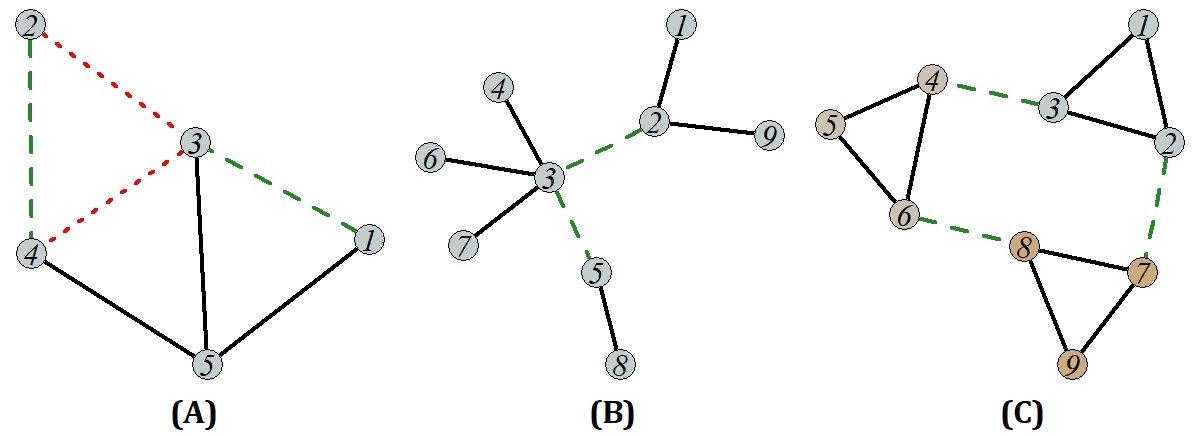
Figure 1: Schematic view of network misspecification. Edges in dashed lines are missing whereas edges in dotted lines are assumed to be present but should be removed. (A) Network with an incorrect list of edges. (B) Network with edges censored at $K=3$. Node $3$ has five edges but two are censored ($2-3,3-5$). (C) Cross-clusters contamination with three clusters.

4.1 Estimation bias

Given the specified network $\boldsymbol{A}^{sp}$, the mean potential outcomes $\mu$ are often estimated by the Horvitz-Thompson (HT) estimator (Ugander et al.,, 2013; Aronow and Samii,, 2017)

$$\hat{\mu}_{\boldsymbol{A}^{sp}}(c_{\ell})=\frac{1}{n}\sum_{i=1}^{n}\frac{\mathbb{I}\{f(\boldsymbol{Z}^{obs},\boldsymbol{A}^{sp}_{i})=c_{\ell}\}}{p_{i}^{(\boldsymbol{A}^{sp})}(c_{\ell})}Y_{i}^{obs}.$$ (3)

Alternatively, the Hajek estimator,

$$\hat{\mu}^{H}_{\boldsymbol{A}^{sp}}(c_{\ell})=\frac{\sum_{i=1}^{n}\frac{\mathbb{I}\{f(\boldsymbol{Z}^{obs},\boldsymbol{A}^{sp}_{i})=c_{\ell}\}}{p_{i}^{(\boldsymbol{A}^{sp})}(c_{\ell})}Y_{i}^{obs}}{\sum_{i=1}^{n}\frac{\mathbb{I}\{f(\boldsymbol{Z}^{obs},\boldsymbol{A}^{sp}_{i})=c_{\ell}\}}{p_{i}^{(\boldsymbol{A}^{sp})}(c_{\ell})}},$$ (4)

was shown to have a better finite-sample accuracy (Särndal et al.,, 2003). Subsequently, $\tau(c_{\ell},c_{k})$ is estimated by the plug-in HT estimator $\hat{\tau}_{\boldsymbol{A}^{sp}}(c_{\ell},c_{k})=\hat{\mu}_{\boldsymbol{A}^{sp}}(c_{\ell})-\hat{\mu}_{\boldsymbol{A}^{sp}}(c_{k})$, and similarly for Hajek estimator $\hat{\tau}^{H}_{\boldsymbol{A}^{sp}}$. Now, the researcher estimates the causal effects with $\boldsymbol{A}^{sp}$, which, as previously indicated, may or may not be in $\mathscr{A}^{\ast}$, i.e., might fail to correctly represent the interference structure. By replacing $Y_{i}^{obs}$ in (3) with its definition under consistency (Assumption 3), we can write the HT estimator as

$$\hat{\mu}_{\boldsymbol{A}^{sp}}(c_{\ell})=\frac{1}{n}\sum_{i=1}^{n}\bigg{[}\underbrace{\frac{\mathbb{I}\{f(\boldsymbol{Z}^{obs},\boldsymbol{A}^{sp}_{i})=c_{\ell}\}}{p_{i}^{(\boldsymbol{A}^{sp})}(c_{\ell})}}_{\text{Selection and weighting}}\underbrace{\sum_{j=1}^{L}\mathbb{I}\{f(\boldsymbol{Z}^{obs},\boldsymbol{A}^{\ast}_{i})=c_{j}\}Y_{i}(c_{j})}_{\text{Observation}}\bigg{]},$$ (5)

where $\boldsymbol{A}^{\ast}$ is some network in $\mathscr{A}^{\ast}$ (Section 3). Equation (5) clarifies that the selection and weighting of units are performed with $\boldsymbol{A}^{sp}$, whereas the observed outcomes are generated by $\mathscr{A}^{\ast}$. Thus, if $\boldsymbol{A}^{sp}\notin\mathscr{A}^{\ast}$, estimation using a misspecified network $\boldsymbol{A}^{sp}$ could yield erroneous results due to selecting the wrong units and weighing their observed outcomes with possibly wrong weights. We now provide a formal result to reflect this intuition.

For exposure values $c_{\ell},c_{k}$ and networks $\boldsymbol{A},\boldsymbol{A}^{\prime}$, define the joint probability that unit $i$ is exposed to $c_{\ell}$ under $\boldsymbol{A}$ and to $c_{k}$ under $\boldsymbol{A}^{\prime}$ by

$$\begin{split}p_{i}^{(\boldsymbol{A},\boldsymbol{A}^{\prime})}(c_{\ell},c_{k})&\vcentcolon=\mathbb{E}_{\boldsymbol{Z}}\Big{[}\mathbb{I}\{f(\boldsymbol{Z},\boldsymbol{A}_{i})=c_{\ell}\}\mathbb{I}\{f(\boldsymbol{Z},\boldsymbol{A}^{\prime}_{i})=c_{k}\}\Big{]}\\ &=\sum_{\boldsymbol{z}\in\mathcal{Z}}\Pr(\boldsymbol{Z}=\boldsymbol{z})\mathbb{I}\{f(\boldsymbol{z},\boldsymbol{A}_{i})=c_{\ell}\}\mathbb{I}\{f(\boldsymbol{z},\boldsymbol{A}^{\prime}_{i})=c_{k}\}.\end{split}$$ (6)

The following theorem shows that the HT estimator $\hat{\tau}_{\boldsymbol{A}^{sp}}$ is a possibly biased estimator of $\tau$, and, given the exposure mapping, the bias depends on the specification of $\boldsymbol{A}^{sp}$ and on the potential outcomes.

Theorem 1.

Let $\boldsymbol{A}^{\ast}$ be an arbitrarily chosen network from $\mathscr{A}^{\ast}$, and let $\boldsymbol{A}^{sp}\in\mathscr{A}$ be a network satisfying Definition 1. Under Assumption 3, for any $c_{\ell},c_{k}$

$$\mathbb{E}_{\boldsymbol{Z}}\Big{[}\hat{\tau}_{\boldsymbol{A}^{sp}}(c_{\ell},c_{k})\Big{]}=\tau(c_{\ell},c_{k})+B(c_{\ell},c_{k};\boldsymbol{A}^{sp}),$$

with $B(c_{\ell},c_{k};\boldsymbol{A}^{sp})=\frac{1}{n}\sum_{i=1}^{n}\sum_{j=1}^{L}\Big{[}q_{i}(c_{j};\boldsymbol{A}^{\ast}|c_{\ell};\boldsymbol{A}^{sp})-q_{i}(c_{j};\boldsymbol{A}^{\ast}|c_{k};\boldsymbol{A}^{sp})\Big{]}Y_{i}(c_{j})$, and where

$$q_{i}(c_{j};\boldsymbol{A}^{\ast}|c_{k};\boldsymbol{A}^{sp})=\begin{cases}\frac{p_{i}^{(\boldsymbol{A}^{\ast},\boldsymbol{A}^{sp})}(c_{j},c_{k})}{p_{i}^{(\boldsymbol{A}^{sp})}(c_{k})},&j\neq k\\ \frac{p_{i}^{(\boldsymbol{A}^{\ast},\boldsymbol{A}^{sp})}(c_{j},c_{k})}{p_{i}^{(\boldsymbol{A}^{sp})}(c_{k})}-1,&j=k\end{cases}$$

Moreover, $B(c_{\ell},c_{k};\boldsymbol{A}^{sp})$ is equal for any $\boldsymbol{A}^{\ast}\in\mathscr{A}^{\ast}$.

Notice that $\frac{p_{i}^{(\boldsymbol{A}^{\ast},\boldsymbol{A}^{sp})}(c_{j},c_{k})}{p_{i}^{(\boldsymbol{A}^{sp})}(c_{k})}$ is the conditional probability that unit $i$ is exposed to $c_{j}$ under $\boldsymbol{A}^{\ast}$, given it is exposed to $c_{k}$ under $\boldsymbol{A}^{sp}$. Thus, the bias of the HT estimator $\hat{\tau}_{\boldsymbol{A}^{sp}}$, as shown in Theorem 1, can be viewed as a linear combination of all potential outcomes with weights that relate to the aforementioned conditional probabilities. Hardy et al., (2019) and Li et al., (2021) derived the bias from using an incorrect network for a specific exposure mapping while assuming $\boldsymbol{A}^{\ast}$ is unique. The following corollary states that the bias is zero when $\boldsymbol{A}^{sp}\in\mathscr{A}^{\ast}$.

Corollary 1.

Under the conditions stated in Theorem 1, if $\boldsymbol{A}^{sp}\in\mathscr{A}^{\ast}$, $\mathbb{E}_{\boldsymbol{Z}}\Big{[}\hat{\tau}_{\boldsymbol{A}^{sp}}(c_{\ell},c_{k})\Big{]}=\tau(c_{\ell},c_{k}),\;\ell,k=1,\dots,L.$

The corollary follows from the fact that if $\boldsymbol{A}^{sp}\in\mathscr{A}^{\ast}$, then in Theorem 1 we can choose $\boldsymbol{A}^{\ast}=\boldsymbol{A}^{sp}$. Thus, the conditional probabilities satisfies $\frac{p_{i}^{(\boldsymbol{A}^{\ast},\boldsymbol{A}^{\ast})}(c_{j},c_{k})}{p_{i}^{(\boldsymbol{A}^{\ast})}(c_{k})}=\mathbb{I}\{j=k\}$, $q_{i}$ are all equal to zero, and $B(c_{\ell},c_{k};\boldsymbol{A}^{\ast})=0$. Ugander et al., (2013) and Aronow and Samii, (2017) proved a similar version of Corollary 1 without considering the class $\mathscr{A}^{\ast}$. Regarding the Hajek estimator (4), being a ratio estimator, it is biased even if $\boldsymbol{A}^{sp}\in\mathscr{A}^{\ast}$, but the bias can be bounded (online Appendix B).

In the specific case of the strong null, $Y_{i}(c_{k})=Y_{i}(c_{\ell})\;(\forall\ell,k$, for all $i$), the interference structure is correctly specified by any network, i.e., $\mathscr{A}^{\ast}=\mathscr{A}$. Thus, Corollary 1 implies that any network structure will yield an unbiased estimation (Sävje et al.,, 2021).

5 Dealing with misspecified interference structure

As established in the previous section, a misspecified network may lead to biased estimation. To address this bias, we suggest solutions for two common scenarios. In the first scenario, the researchers have a collection of possible networks but are unsure which is the correct one. Section 5.1 presents an estimator that simultaneously incorporates multiple networks and is unbiased if one of them is correctly specified. In the second scenario, the researchers have a single network but suspect it might be misspecified. For this scenario, Section 5.2 introduces a sensitivity analysis framework.

5.1 Network-misspecification-robust estimator

Assume that a researcher has a collection $\mathcal{A}$ of $M$ possible networks but is uncertain which of the networks in $\mathcal{A}$, if any, correctly specify the interference structure. Typically, $\mathcal{A}$ includes networks that are natural to consider (e.g., different encoding of questionnaire answers). Define $I_{i}^{(\mathcal{A})}(\boldsymbol{Z},c_{\ell})=\prod_{\boldsymbol{A}\in\mathcal{A}}\mathbb{I}\{f(\boldsymbol{Z},\boldsymbol{A}_{i})=c_{\ell}\}$ to be the indicator that equals to one only if the exposure value equals to $c_{\ell}$ under each of the networks in $\mathcal{A}$. Extending the joint probability (6), we define the joint probability that unit $i$ has exposure value $c_{\ell}$ under all $\boldsymbol{A}\in\mathcal{A}$ by $p_{i}^{(\mathcal{A})}(c_{\ell})\vcentcolon=\mathbb{E}_{\boldsymbol{Z}}\left[I_{i}^{(\mathcal{A})}(\boldsymbol{Z},c_{\ell})\right].$ Our proposed modified HT estimator of $\mu(c_{\ell})$ that simultaneously utilizes the $M$ different networks is

$$\hat{\mu}_{\mathcal{A}}(c_{\ell})=\frac{1}{n}\sum_{i=1}^{n}\frac{I_{i}^{(\mathcal{A})}(\boldsymbol{Z}^{obs},c_{\ell})}{p_{i}^{(\mathcal{A})}(c_{\ell})}Y_{i}^{obs}.$$ (7)

That is, $\hat{\mu}_{\mathcal{A}}(c_{\ell})$ selects only units that has exposure value $c_{\ell}$ under all the networks in $\mathcal{A}$ and weights them with the inverse of the joint probability $p_{i}^{(\mathcal{A})}(c_{\ell})$. The modified estimator of the causal effects $\tau(c_{k},c_{\ell})$ is the plug-in estimator $\hat{\tau}_{\mathcal{A}}(c_{\ell},c_{k})=\hat{\mu}_{\mathcal{A}}(c_{\ell})-\hat{\mu}_{\mathcal{A}}(c_{k})$. As we now show, $\hat{\tau}_{\mathcal{A}}$ is an unbiased estimator of $\tau$ if at least one of the networks in $\mathcal{A}$ correctly specifies the interference structure.

Theorem 2.

Let $\mathcal{A}$ be a collection of $M$ networks such that each of the networks satisfies Definition 1. Under Assumption 3, if $\mathcal{A}\cap\mathscr{A}^{\ast}\neq\emptyset$, then

$$\mathbb{E}_{\boldsymbol{Z}}\Big{[}\hat{\tau}_{\mathcal{A}}(c_{\ell},c_{k})\Big{]}=\tau(c_{\ell},c_{k}),\;\ell,k=1,\dots,L.$$

The key property of the estimator $\hat{\tau}_{\mathcal{A}}$ is that by selecting only units with the same exposure values under each of the networks in $\mathcal{A}$, we are guaranteed to observe the correct exposure values if one of the networks is correctly specified, but agnostic to which network it is. Therefore, we term $\hat{\tau}_{\mathcal{A}}$ a network misspecification robust (NMR) estimator. Similarly to $\hat{\mu}_{\mathcal{A}}$, we also propose the NMR Hajek estimator

$$\hat{\mu}^{H}_{\mathcal{A}}(c_{\ell})=\frac{\sum_{i=1}^{n}\frac{I_{i}^{(\mathcal{A})}(\boldsymbol{Z}^{obs},c_{\ell})}{p_{i}^{(\mathcal{A})}(c_{\ell})}Y_{i}^{obs}}{\sum_{i=1}^{n}\frac{I_{i}^{(\mathcal{A})}(\boldsymbol{Z}^{obs},c_{\ell})}{p_{i}^{(\mathcal{A})}(c_{\ell})}}.$$ (8)

$\hat{\mu}^{H}_{\mathcal{A}}$ selects the same subset of units as $\hat{\mu}_{\mathcal{A}}$, but is biased since it is a ratio estimator (Särndal et al.,, 2003). In online Appendix B we derive the bias bounds. In the simulation study (Section 6.1), we found that HT and Hajek NMR estimators had a similar bias.

The NMR estimators offer greater flexibility in the network selection as they allow simultaneously taking any combination of networks. However, this flexibility poses a bias-variance tradeoff. Using more networks (large $M$) can lower the bias (if a correct network is included), but it also increases variance due to the reduction in the number of units used and the joint probabilities $p_{i}^{(\mathcal{A})}$ values. The tradeoff magnitude depends on the number of networks and their relative similarity. In Section 6.2, we illustrate this bias-variance tradeoff via a simulation study.

We now discuss how the NMR estimator can be applied in some of the previously discussed examples.

Example 1 (continued).

When data on social connections from different reporting is available (e.g., by asking different questions in the questionnaire), multiple networks can be derived. If the researchers are unsure which of the networks is correctly specified, they can estimate the causal effects with the NMR estimator taking all the networks simultaneously.

Example 3 (continued).

When the researchers are not sure which type of reciprocity is relevant, the estimation can be done with the NMR estimator that simultaneously utilizes all available networks from all possible reciprocity choices.

Example 4 (continued).

When networks are specified from data gathered in different time periods, the researchers can estimate the causal effect with the NMR estimator and all the networks together.

In Section 7.1 we apply the NMR estimator to a social network field experiment in which four available networks can be derived from two different questions in questionnaires that are measured in two time periods, thus highlighting Examples 1 and 4.

Building on previous work (Aronow and Samii,, 2013) based on Young’s inequality, we derive a conservative variance estimator $\savestack{\tmpbox}{\stretchto{\scaleto{\scalerel*[\widthof{Var}]{\kern-0.6pt\bigwedge\kern-0.6pt}{\rule[-628.74876pt]{4.30554pt}{628.74876pt}}}{}}{0.5ex}}\stackon[1pt]{Var}{\tmpbox}\big{(}\hat{\tau}_{\mathcal{A}}\big{)}$, i.e., its expected value is not smaller than $Var_{\boldsymbol{Z}}\big{(}\hat{\tau}_{\mathcal{A}}\big{)}$. Variance estimation of Hajek NMR is similarly obtained with Taylor linearization. Full details are provided in online Appendix C. In online Appendix F, we demonstrate in simulations the conservativeness property.

5.2 Sensitivity analysis

When researchers doubt whether the specified network $\boldsymbol{A}^{sp}$ correctly represents the interference structure, investigating the sensitivity of the causal estimates to deviations from $\boldsymbol{A}^{sp}$ is of great interest. To that end, we propose a sensitivity analysis for the specified network. Our proposal builds on the idea that misspecification concerns can be represented by a probability distribution.

The researchers represent their suspected deviations from $\boldsymbol{A}^{sp}$ by a probability distribution $P_{\theta}$. Formally, this distribution is the conditional distribution $\boldsymbol{A}^{\theta}|\boldsymbol{A}^{sp}\sim P_{\theta}$ for some parameter $\theta$. For each $\theta$ value, the random variable $\boldsymbol{A}^{\theta}$ can be viewed as a random network obtained by perturbing $\boldsymbol{A}^{sp}$. For example, if $\theta_{t}=\Pr(A^{\theta}_{ij}=1-t|A^{sp}_{ij}=t),\;t\in\{0,1\}$, then $P_{\theta}$ is an induced distribution that randomly removes each of the edges in $\boldsymbol{A}^{sp}$ with probability $\theta_{1}$ and adds an edge that is not present in $\boldsymbol{A}^{sp}$ with probability $\theta_{0}$ (per edge). E.g., a value of $\theta_{1}=0.01$ implies that about $1$ out of $100$ assumed edges are incorrect. It is also possible to take $P_{\theta}=P_{\theta}(\boldsymbol{x})$ for covariates $\boldsymbol{x}$ thus allowing for data-based heterogeneity in $P_{\theta}$, as we discuss in the examples below.

Let $\hat{\tau}_{\boldsymbol{A}^{\theta}}$ be the causal effect estimates when replacing $\boldsymbol{A}^{sp}$ with $\boldsymbol{A}^{\theta}$. Given the observed treatments $\boldsymbol{Z}^{obs},$ the estimators $\hat{\tau}_{\boldsymbol{A}^{\theta}}$ are functions of the random variable $\boldsymbol{A}^{\theta}$ and are thus random. That is, $P_{\theta}$ gives rise for a distribution of $\hat{\tau}_{\boldsymbol{A}^{\theta}}$ as a function of $\theta$, which is obtained by perturbing $\boldsymbol{A}^{sp}$ with the induced distribution $P_{\theta}$. Thus, learning about the distribution of $\hat{\tau}_{\boldsymbol{A}^{\theta}}$ is akin to understanding how sensitive the estimates are to deviations from $\boldsymbol{A}^{sp}$.

However, given $P_{\theta}$, deriving the closed-form distribution of $\hat{\tau}_{\boldsymbol{A}^{\theta}}$ is not possible in general, and obtaining all the networks in $\boldsymbol{A}^{\theta}$ domain is computationally infeasible, therefore an approximation is required. To this end, we propose a Monte Carlo routine. For a given parameter value $\theta$ and $B$ number of draws, the routine is as follows.

1. Repeat for $b=1,\dots,B$

   1. Sample $\boldsymbol{A}^{\theta,b}|\boldsymbol{A}^{sp}\sim P_{\theta}$.

   2. Calculate $\hat{\tau}_{\boldsymbol{A}^{\theta,b}}(c_{\ell},c_{k}),\;\ell,k=1,\dots,L$.

2. Return $\Big{\{}\hat{\tau}_{\boldsymbol{A}^{\theta,b}}\Big{\}}_{b=1}^{B}$.

The HT estimator $\hat{\tau}_{\boldsymbol{A}^{\theta}}$ in Step 1(b) can be replaced with the Hajek estimator $\hat{\tau}^{H}_{\boldsymbol{A}^{\theta}}$. A natural way to display the results is by plotting the distribution of $\hat{\tau}_{\boldsymbol{A}^{\theta}}$ for a sequence of $\theta$ values and comparing it with the estimate $\hat{\tau}_{\boldsymbol{A}^{sp}}$. Alternatively, summary measures of $\hat{\tau}_{\boldsymbol{A}^{\theta}}$ can be presented (e.g., mean, median, other quantiles, or maximal and minimal values).

To illustrate the practical utility of the proposed sensitivity analysis, consider again the previously mentioned examples.

Examples 1-2 (continued). Inspecting how sensitive the causal estimates are to possible incorrect reporting of social connections (Example 1) can be accomplished by postulating that a proportion of edges are missing or superfluous. For example, as previously discussed, the researchers can take $P_{\theta}=(\theta_{0},\theta_{1})$ where $\theta_{t}=\Pr(A_{ij}^{\theta}=1-t|A^{sp}_{ij}=t)$. When the concern is censoring of edges (Example 2), the researchers can take $\theta_{1}=0$ and $\theta_{0}>0$ only for units with degrees equal to the censoring threshold.

Example 5 (continued). Studying how causal estimates are sensitive to cross-clusters contamination can be performed by letting $P_{\theta}$ represent the distribution of cross-clusters edge creations. For example, by postulating that the probability of cross-clusters contamination is inversely related to the spatial distance between clusters, the researchers can take $P_{\theta}=P_{\theta}(\boldsymbol{x})$ for a spatial measure $\boldsymbol{x}$.

In Section 7.2 we apply the sensitivity analysis for a cluster-randomized trial (CRT) (Venturo-Conerly et al.,, 2022) in which cross-clusters contamination is suspected.

6 Simulations

We performed a simulation study consisting of two parts. Section 6.1 illustrates the bias resulting from using a misspecified network. Section 6.2 shows the bias-variance tradeoff of the NMR estimators in practice.

For all simulations, the exposure mapping was defined as follows. For network $\boldsymbol{A}$ and binary treatment vector $\boldsymbol{z}$, denote the proportion of treated neighbors of unit $i$ by $g(\boldsymbol{z},\boldsymbol{A}_{i})=\lvert\mathcal{N}_{i}(\boldsymbol{A})\rvert^{-1}\sum_{j=1}^{n}A_{ij}z_{j}$. The heterogeneous thresholds exposure mapping is defined by

$$f(\boldsymbol{z},\boldsymbol{A}_{i})=\begin{cases}c_{11},&z_{i}\cdot\mathbb{I}\{g(\boldsymbol{z},\boldsymbol{A}_{i})>\nu_{i}\}=1\\[-10.0pt] c_{01},&(1-z_{i})\cdot\mathbb{I}\{g(\boldsymbol{z},\boldsymbol{A}_{i})>\nu_{i}\}=1\\[-10.0pt] c_{10},&z_{i}\cdot(1-\mathbb{I}\{g(\boldsymbol{z},\boldsymbol{A}_{i})>\nu_{i}\})=1\\[-10.0pt] c_{00},&(1-z_{i})\cdot(1-\mathbb{I}\{g(\boldsymbol{z},\boldsymbol{A}_{i})>\nu_{i}\})=1,\end{cases}$$ (9)

where $\nu_{i}\in[0,1)$ is a known, possibly unit-specific, threshold. The exposure mapping (9) implies the exposure is a result of two components: whether unit $i$ is treated, and whether the proportion of its treated neighbors surpassed the threshold $\nu_{i}$. If it is further assumed that $\nu_{i}=0\;\forall i,$ (9) reduces to a commonly used exposure mapping (Aronow and Samii,, 2017). We generated the potential outcomes by taking $Y_{i}(c_{00})\sim U[0.5,1.5]$ and $Y_{i}(c_{11})=2\cdot Y_{i}(c_{00}),\;Y_{i}(c_{10})=1.5\cdot Y_{i}(c_{00}),\;Y_{i}(c_{01})=1.25\cdot Y_{i}(c_{00})$. Thresholds were sampled from $\nu_{i}\sim U[0,1]$ and are assumed to be known. Treatment assignment mechanisms varied between the different scenarios; details are given below. All simulations were repeated for $1000$ iterations in each setup. We present and discuss our main findings. Additional details, specifications, results, and a study focused on the proposed conservative variance estimators are all provided in online Appendix F.

6.1 Illustrations of the estimation bias

We considered three scenarios of network misspecification: incorrect reporting of social connections (Example 1); censoring (Example 2); and cross-clusters contamination (Example 5). In the first two scenarios, we examined how estimating the causal effects using misspecified networks biases the results. For the contamination scenario, we studied the bias resulting from naively assuming the structure of well-separated clusters (i.e., partial interference) when cross-clusters contamination is present.

Scenario (I) (Incorrect reporting of social connections).

A single true network $\boldsymbol{A}^{\ast}$ was sampled from a preferential attachment (PA) random network (Barabási and Albert,, 1999) with $n=3000$ nodes. We created several misspecified networks $\widetilde{\boldsymbol{A}}$ by independently adding and removing edges from $\boldsymbol{A}^{\ast}$ with probability $\eta_{1-t,t}=\Pr(\widetilde{A}_{ij}=1-t|A^{\ast}_{ij}=t),\;t=0,1$, for $i\neq j$. We took $\eta:=\eta_{0,1}$, fixed $\eta_{1,0}=\eta/100$, and repeated for $\eta\in\{0.025,\dots,0.25\}$. Treatments were assigned with Bernoulli allocation $\Pr(\boldsymbol{Z}=\boldsymbol{z})=0.5^{n}$. For each $\eta$ value we generated one misspecified network and used it for the estimation of causal effects.

Scenario (II) (Censoring).

For the same $\boldsymbol{A}^{\ast}$ as in Scenario (I), the censoring of edges in $\boldsymbol{A}^{\ast}$ was obtained by randomly removing edges of units with more than $K$ edges to obtain a maximum degree of $K\in\{1,\dots,7\}$. Treatments were assigned with Bernoulli allocation. For each $K$ value, one censored network was created and used in the estimation.

Scenario (III) (Cross-clusters contamination).

We illustrate the impact of contamination in spatial settings. We sampled $V$ clusters uniformly on the unit cube $[0,1]^{2}$ such that each cluster is fully connected. Let $\boldsymbol{A}^{CRT}$ denote the resulting network. Let $d(v,v^{\prime})=\lVert v_{c}-v_{c}^{\prime}\rVert_{L_{1}}$ be the spatial distance between clusters $v$ and $v^{\prime}$ with $v_{c}$ being the coordinates of cluster $v$. Contamination is generated by letting two units in clusters $v\neq v^{\prime}$ form an edge independently with probability $p_{v,v^{\prime}}(\gamma)=\exp\left(-\frac{d(v,v^{\prime})}{\gamma\cdot\bar{D}}\right)$, where $\bar{D}=\binom{V}{2}^{-1}\sum_{v\neq v^{\prime}}d(v,v^{\prime})$ is the mean of pairwise clusters distances and $\gamma\geq 0$ controls the magnitude, i.e., $p_{v,v^{\prime}}(\gamma)$ is monotonically increasing in $\gamma$. We let $p_{v,v^{\prime}}(0)=\mathbb{I}\{v=v^{\prime}\}$. Thus, $p_{v,v^{\prime}}$ decays as the distance between clusters increases. For each $\gamma$ value we created one contaminated network $\boldsymbol{A}^{\ast}$, according to which the potential outcomes were generated. We studied how wrongly assuming no contamination ($\boldsymbol{A}^{CRT}$) biases the overall treatment effect $\tau(c_{11},c_{00})$. Clusters were independently assigned to treatment with probability $0.5$. We repeated the simulation for $V=500$ clusters of $20$ units each (fixed sizes), and for $V=2000$ clusters with sizes between $3$ and $7$ (varied sizes).

Figure 2 displays the relative bias in each of the three scenarios. For Scenarios (I)-(II), we report here the results for the HT (3) and Hajek (4) estimators of the direct effect $\tau(c_{10},c_{00})$. For Scenario (I), the magnitude of misspecification was controlled by $\eta$. When $\eta=0$, the true network was used, and, as expected from Corollary 1, the bias was close to zero. As one might expect, the relative bias increased with $\eta$. In Scenario (II), as the censoring threshold $K$ decreased, the censoring increased, and accordingly so was the bias. Turning to Scenario (III), when there was no contamination ($\gamma=0$) the bias was around zero, and as contamination increased the bias grew as well. In both Scenarios (I) and (II), the relative bias was larger for the indirect effects $\tau(c_{01},c_{00})$ and $\tau(c_{11},c_{10})$ (online Appendix F). These results can be intuitively explained by recognizing that, under the exposure mapping (9), network misspecification may lead us to classify a person with true exposure level $c_{j0}$ to exposure level $c_{j1}$ (and vice versa), but will not affect $j$.

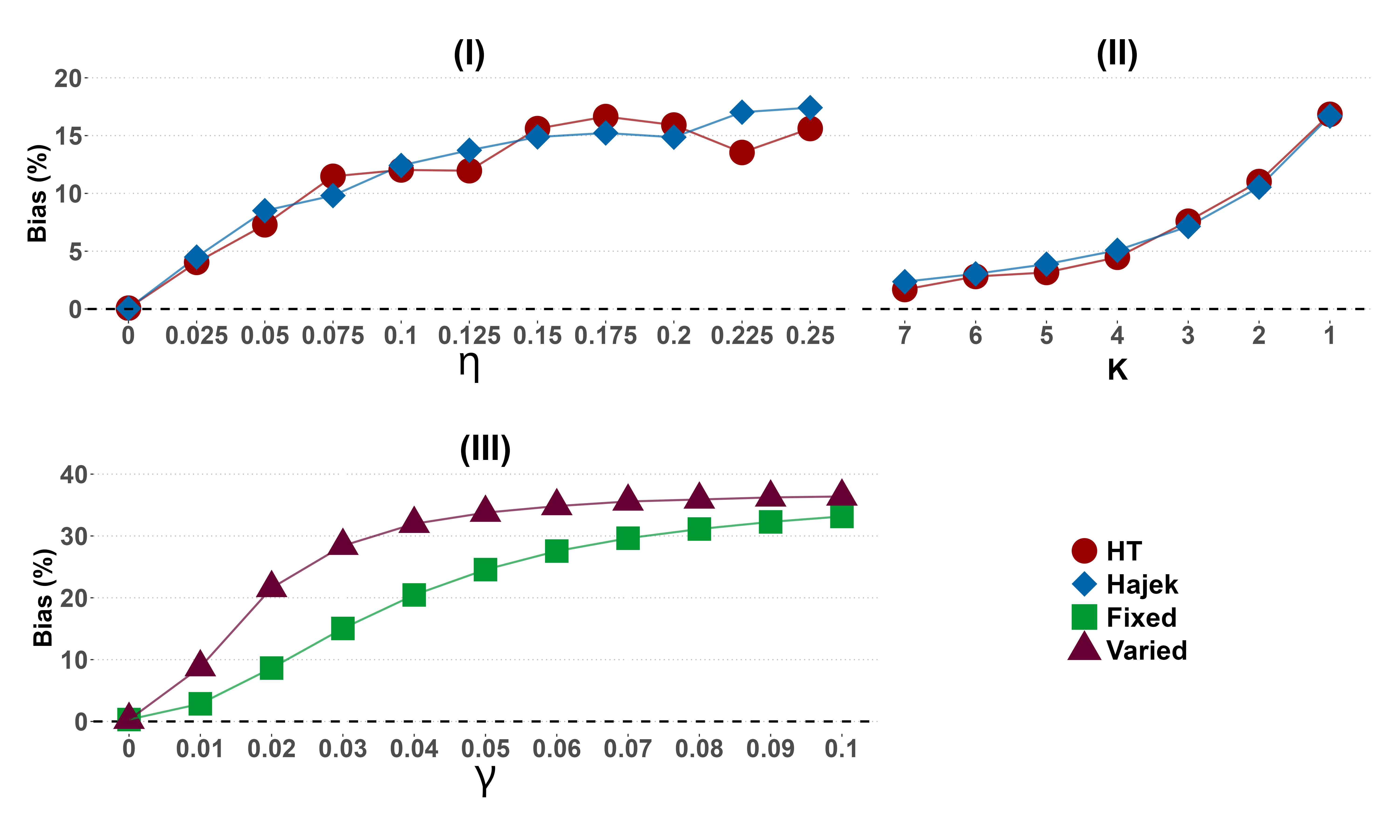
Figure 2: Relative bias $(100(mean(\hat{\tau})-\tau)/\tau)$ due to misspecified network. In Scenarios (I) and (II), $\tau(c_{10},c_{00})$ was estimated with both HT (circles) and Hajek (diamonds) estimators. In Scenario (I), $\eta$ controls the misspecification level. In Scenario (II), $K$ is the censoring threshold. Scenario (III) shows how contamination level $\gamma$ impacts the bias of $\tau(c_{11},c_{00})$ in a CRT with fixed (squares) and varied (triangles) clusters size. True causal effects are $\tau(c_{10},c_{00})=0.5,\tau(c_{11},c_{00})=1$.

6.2 Bias-variance tradeoff of the NMR estimators

The second simulation study illustrates the bias-variance tradeoff of the NMR estimators. Taking the true network $\boldsymbol{A}^{\ast}$ to be the same as in Scenarios (I) and (II) of Section 6.1, we generated from $\boldsymbol{A}^{\ast}$ five misspecified networks $\boldsymbol{A}^{a},\dots,\boldsymbol{A}^{e}$ by independently adding and removing edges using $\eta_{0,1}=0.25$ and $\eta_{1,0}=\eta_{0,1}/100$ with $\eta_{1-t,t}$ as defined in Section 6.1. In total, there were six available networks. After assigning treatments with Bernoulli allocation, we calculated the NMR estimators under each of the $\binom{6}{M}$ possible combinations of $\mathcal{A}$ specifications for each $M=1,\dots,6$. For example, if $M=2$, these possible $\mathcal{A}$ combinations are $\bigg{\{}\{\boldsymbol{A}^{\ast},\boldsymbol{A}^{a}\},\{\boldsymbol{A}^{\ast},\boldsymbol{A}^{b}\},\dots,\{\boldsymbol{A}^{d},\boldsymbol{A}^{e}\}\bigg{\}}$.

Figure 3 shows the relative bias, standard deviation (SD), and root-mean-squared-error (RMSE) of the Hajek NMR estimator for $\tau(c_{11},c_{10})$. The bias was practically zero whenever $\boldsymbol{A}^{\ast}\in\mathcal{A}$, and larger than zero when it was not the case. The SD increased with $M$, regardless if $\boldsymbol{A}^{\ast}$ was included or not, due to the smaller effective sample size. Results for additional estimands and measures of the networks’ similarity can be found in online Appendix F. The results are qualitatively the same as those reported here.

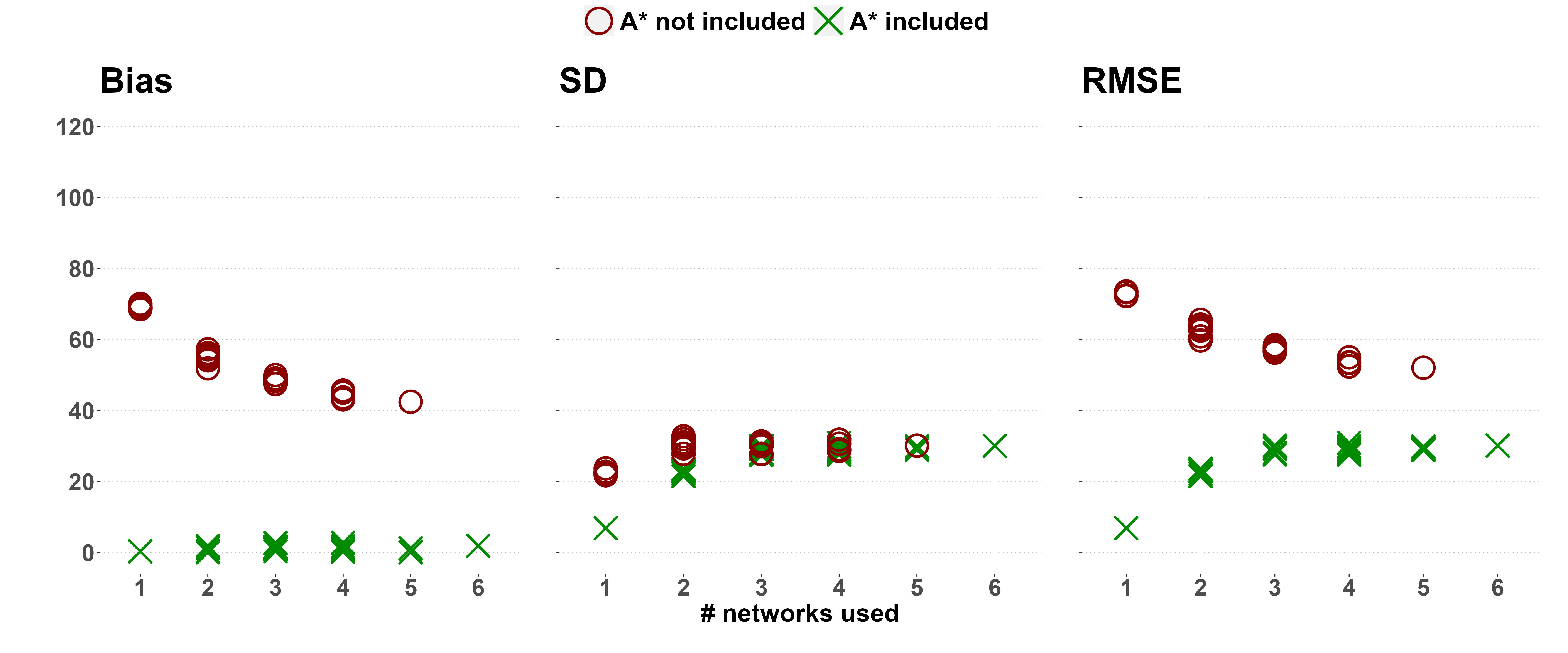
Figure 3: Bias-variance tradeoff of the NMR Hajek estimator for $\tau(c_{11},c_{10})$ as captured by bias, SD, and RMSE (all reported in % relative to the true $\tau(c_{11},c_{10})$ for ease of presentation). $X$’s indicate that the true network $\boldsymbol{A}^{\ast}$ is included in $\mathcal{A}$, and $O$’s otherwise. True causal effect is $\tau(c_{11},c_{10})=0.5$.

7 Data analyses

7.1 Social network field experiment

We analyzed a field experiment that tested how anti-conflict norms spread in middle school social networks. Key information is provided below; full details are given in Paluck et al., (2016). Following previous analyses (Aronow and Samii,, 2017), we analyzed a subset of $n=2983$ eligible students from $56$ schools. Half of the schools were randomly assigned to the intervention arm, and within each selected school, half of the eligible students were given a year-long anti-conflict educational intervention. To derive the within-school social network, students were asked to list ten students they spend time (ST) with. The questionnaires were given during the pre- and post-intervention periods. As previously discussed (Example 4), a social network of middle school students is dynamic and probably changed in the span of a year. Moreover, students’ questionnaire answers might not be an accurate representation of the interference structure (Example 1). Specifically, students were also asked to list their two best friends (BF). A network structure based on this list is different from the network structure derived from the ST list. Thus, the researchers can choose between four different network specifications: either the ST or BF networks from either the measurement in the pre- or post-intervention periods.

We proceed to estimate the effect of the intervention on a behavior outcome (an indicator of wearing a wristband endorsing the program). Following Aronow and Samii, (2017), we use the exposure mapping defined below, which is in the nature of (9), but also indicates whether the school was assigned to the intervention arm. Let $s_{i}$ be an indicator of whether the school of unit $i$ was included in the intervention arm. The exposure mapping is

$$f(\boldsymbol{z},\boldsymbol{A}_{i})=\begin{cases}c_{111},&z_{i}\mathbb{I}\{g(\boldsymbol{z},\boldsymbol{A}_{i})>0\}s_{i}=1\\[-10.0pt] c_{011},&(1-z_{i})\mathbb{I}\{g(\boldsymbol{z},\boldsymbol{A}_{i})>0\}s_{i}=1\\[-10.0pt] c_{101},&z_{i}(1-\mathbb{I}\{g(\boldsymbol{z},\boldsymbol{A}_{i})>0\})s_{i}=1\\[-10.0pt] c_{001},&(1-z_{i})(1-\mathbb{I}\{g(\boldsymbol{z},\boldsymbol{A}_{i})>0\})s_{i}=1\\[-10.0pt] c_{000},&(1-s_{i})=1\end{cases}$$

In our analysis, we estimated the causal effects with each of the four networks separately, and with all four networks simultaneously with the NMR estimators.

Table 1 displays the estimated school participation effect $\tau(c_{001},c_{000})$ and the direct isolated effect $\tau(c_{101},c_{000})$ coupled with conservative standard errors (SEs) estimates. The BF network resulted in a larger estimated SE than the ST network due to the sparser network structure. The Hajek point estimates were larger and had smaller SEs than HT estimators across all setups. A surprising result is that for the Hajek estimator, the point estimates were similar using the four networks separately and simultaneously, but those estimates varied more in HT, perhaps due to the instability of the weights. Looking at the Hajek estimates, we can conclude that both $\tau(c_{001},c_{000})$ and $\tau(c_{101},c_{000})$ were found to have a small positive value, and the results were robust to the four possible specifications of the network structure. Results from different network combinations and on additional estimands are given in online Appendix F.

	$\tau(c001,c000)$		$\tau(c101,c000)$
Networks	HT	Hajek	HT	Hajek
ST-pre	0.061 (0.217)	0.146 (0.164)	0.096 (0.272)	0.271 (0.19)
BF-pre	0.084 (0.254)	0.123 (0.195)	0.169 (0.361)	0.265 (0.254)
ST-post	0.06 (0.214)	0.131 (0.164)	0.116 (0.298)	0.252 (0.212)
BF-post	0.09 (0.262)	0.135 (0.2)	0.17 (0.362)	0.258 (0.256)
ALL	0.04 (0.177)	0.178 (0.131)	0.046 (0.19)	0.227 (0.137)

Table 1: Estimated causal effects in the social network field experiment. Results are reported as point estimates (SE). “ALL” is the four networks combined and is estimated with the NMR estimators.

7.2 Cluster-randomized trial

We analyzed a CRT that tested how educational intervention affects depression and anxiety symptoms among secondary school students in Kenya (Venturo-Conerly et al.,, 2022). The study included $895$ students from two schools with $12$ classes each. Classes were randomly assigned to one of four different treatment arms: Growth, Value, Gratitude, and Control. The outcomes are the differences in the Generalized Anxiety Disorder Screener (GAD) and the Patient Health Questionnaire (PHQ) metrics. The experiment consisted of a single-session educational intervention followed by a re-measurement of GAD and PHQ two weeks later. Venturo-Conerly et al., (2022) found a significant effect only with the Growth and Value interventions, thus we defined binary treatment $z_{i}$ that equal to one only if student $i$ was assigned to Growth or Value interventions.

We addressed the concern that students from different classes, at the same school, can interact and share insights from the intervention, thus leading to contamination between clusters (classes). Therefore, we applied the sensitivity analysis proposed in Section 5.2 to examine how cross-clusters contamination may have changed the results. The baseline network $\boldsymbol{A}^{CRT}$ has the structure of $24$ well-separated clusters, where all units are fully connected within each cluster. Contamination is postulated to be possible only within the school and is represented by the cross-clusters edge creation probability $\theta=\Pr(A_{ij}=1|A^{CRT}_{ij}=0)$ for units $i,j$ that are in different classes but in the same school, and $\boldsymbol{A}$ is the contaminated network. We assumed the exposure mapping (9) with $\nu_{i}=0$ and focused on estimating the overall treatment effect $\tau(c_{11},c_{00})$ (see online Appendix D for more details on estimands in CRTs).

Figure 4 displays the distribution of point estimates from the sensitivity analysis for $\theta=0,\dots,0.01$ with $500$ Monte Carlo iterations per $\theta$ value. This choice of $\theta$ values reflects a belief that up to $1\%$ of the edges assumed to be absent may in fact exist. Estimates (SE) assuming no contamination for GAD and PHQ were $-0.97\;(0.3)$ and $-0.65\;(0.18)$, respectively. For both outcomes, the median estimate over the different networks was relatively stable across all $\theta$ values. However, as $\theta$ increased, the estimates for more networks crossed zero and changed sign, thus the estimated effects when assuming no-contamination might be diluted. Since the network-related uncertainty in the estimates increased with $\theta$, we can conclude that the estimates assuming no contamination should be interpreted with caution.

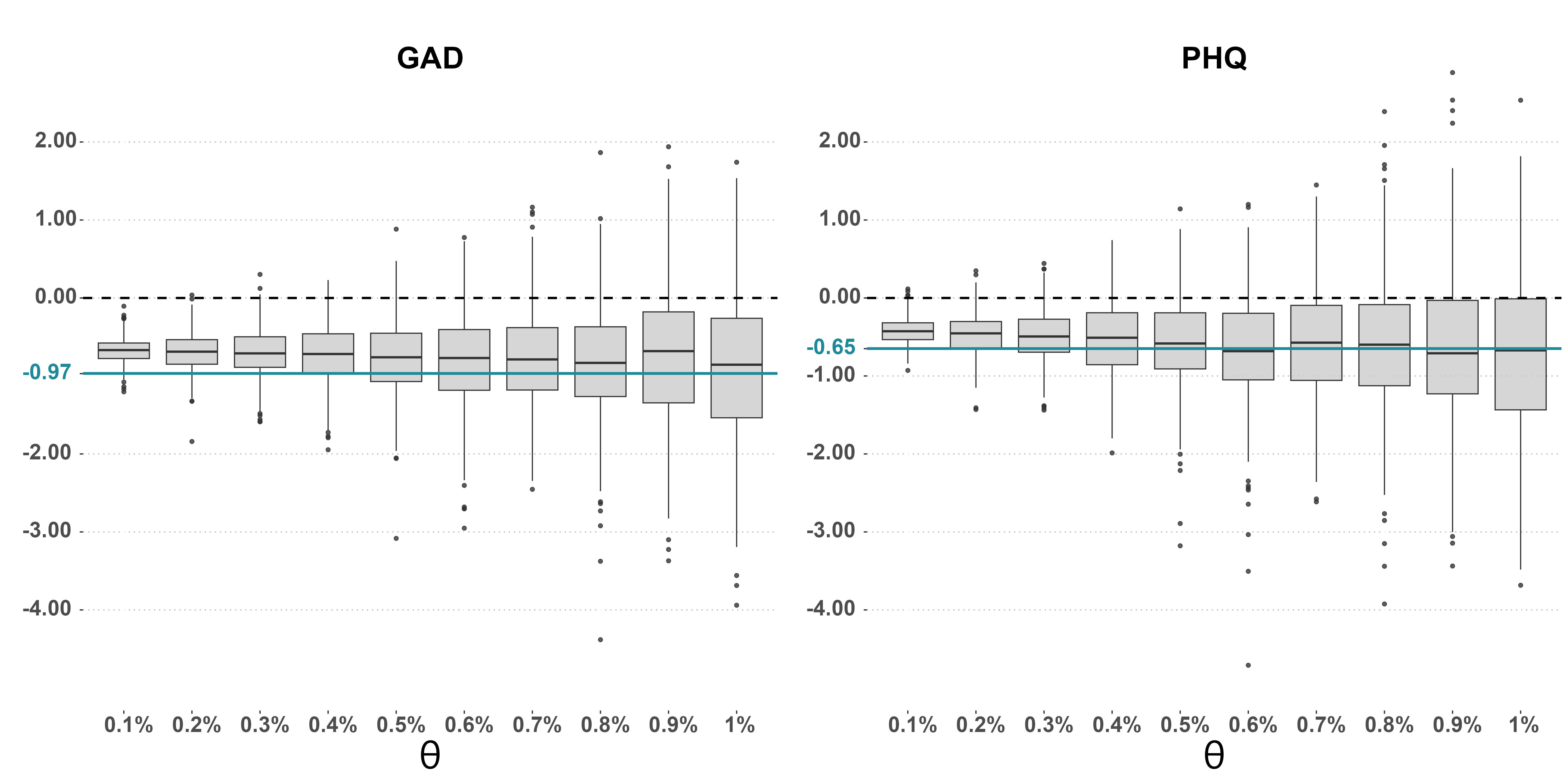
Figure 4: Sensitivity analysis for cross-clusters contamination in an educational intervention CRT. $\theta$ is the between-clusters’ contamination probability. The boxplots visualize the distribution of point estimates across $500$ iterations. Estimates assuming no contamination are displayed as solid horizontal lines.

8 Discussion

In this paper, we studied the estimation of causal effects with a misspecified network interference structure. Building on the exposure mapping framework, we found that the correctly specified network is not necessarily unique, and that uniqueness is guaranteed under certain conditions. Motivated by our results on the bias arising from using a wrong network, we proposed two practical solutions. We first proposed the NMR estimator that allows estimation using multiple networks simultaneously and showed that it is unbiased if at least one of the networks is correctly specified. The bias-variance tradeoff of the NMR estimators was demonstrated in a simulation study. As a second practical tool, we also proposed a sensitivity analysis framework when researchers have a single network and can postulate a suspected misspecification mechanism. Such an approach is attractive when researchers have in mind potential deviations from the assumed network and would like to examine the sensitivity of their estimates to these deviations. One prominent scenario is a CRT with possible cross-clusters contamination, for which we provided a data analysis example illustrating our proposed approach.

In the simulation study, we considered the heterogeneous thresholds exposure mapping (9). Estimation of the thresholds is an interesting area for future research and has only been done in linear parametric settings (Tran and Zheleva,, 2022). Furthermore, throughout the paper, we assumed that the exposure mapping is correctly specified (Aronow and Samii,, 2017; Sävje,, 2021). Accounting for both misspecified exposure mapping and network interference structure is an important area for future research.

Misspecification of the interference network might result from a partial set of nodes (units) or from an incorrect set of edges (for a given set of nodes). Using a subsample of units in a network yields a bias even when treatment is randomized (Chandrasekhar and Lewis,, 2011). In this paper, we focused only on the impact of an incorrect set of edges. Causal inference with misspecification of the network’s structure due to missing nodes is another area for future research.

Recent literature suggests that unbiased and consistent estimation of the total treatment effect is possible even when no network interference structure is available (Sävje et al.,, 2021; Cortez et al.,, 2022; Yu et al.,, 2022). However, studying more intricate channels of interference requires a network measurement (Yu et al.,, 2022).

Interference is the norm rather than the exception in many social domains, such as economics, political science, sociology, and infectious disease epidemiology. However, causal inference with interference raises various technical and conceptual difficulties. To address these challenges, rigorous applications must acknowledge and address the limitations that arise from interference. Our work is a step towards achieving this goal.

Online Appendix

Appendix A Proofs

A.1 Proof of Proposition 1

Proof.

Assume in contradiction there exists another network $\boldsymbol{A}\in\mathscr{A}$ that satisfies Definition 2, which is not $\boldsymbol{A}^{\ast}$ (i.e., $\boldsymbol{A}^{\ast}\neq\boldsymbol{A}$). Assumption 1 implies there exists $\boldsymbol{z}\in\mathcal{Z}$ such that $f(\boldsymbol{z},\boldsymbol{A}^{\ast}_{i})=c_{\ell}$ and $f(\boldsymbol{z},\boldsymbol{A}_{i})=c_{k}$, for some $i$ and some $\ell\neq k$. By Definition 2, we have that $Y_{i}(\boldsymbol{z})=Y_{i}(c_{\ell})$ and $Y_{i}(\boldsymbol{z})=Y_{i}(c_{k})$, i.e., $Y_{i}(c_{\ell})=Y_{i}(c_{k})$. However this is in contradiction to Assumption 2, thus it must be that $\boldsymbol{A}^{\ast}=\boldsymbol{A}$. ∎

A.2 The heterogeneous thresholds exposure mapping satisfies Assumption 1

Proposition A.1.

Assumption 1 holds for the exposure mapping (9).

Proof.

Let $\boldsymbol{A}\neq\boldsymbol{A}^{\prime}\in\mathscr{A}$. Since $\boldsymbol{A}\neq\boldsymbol{A}^{\prime}$, there exists some unit $i$ with $\boldsymbol{A}_{i}\neq\boldsymbol{A}^{\prime}_{i}$. The difference between $\boldsymbol{A}_{i}$ and $\boldsymbol{A}^{\prime}_{i}$ can be due to the addition or removal of at least one edge. Let $d_{i}(\boldsymbol{A})=|\mathcal{N}_{i}(\boldsymbol{A})|$ be the degree of unit $i$ in network $\boldsymbol{A}$. Assume that $d_{i}(\boldsymbol{A})=a$ and $d_{i}(\boldsymbol{A}^{\prime})=a^{\prime}$, for some scalars $a,a^{\prime}\in\mathbb{N}$. Assume WLOG that $a\geq a^{\prime}$.

Denote the set of joint edges of $i$ in the two networks by $\mathcal{M}_{i}(\boldsymbol{A},\boldsymbol{A}^{\prime})=\mathcal{N}_{i}(\boldsymbol{A})\cap\mathcal{N}_{i}(\boldsymbol{A}^{\prime})$. Denote the complementary set of $\mathcal{N}_{i}(\boldsymbol{A})$, excluding $i$ itself, by $\mathcal{N}_{i}(\boldsymbol{A})^{c}=\{j\neq i:A_{ij}=0\}$, and similarly for $\mathcal{N}_{i}(\boldsymbol{A}^{\prime})^{c}$. Denote the edges difference set by $\mathcal{N}_{i}(\boldsymbol{A})\setminus\mathcal{N}_{i}(\boldsymbol{A}^{\prime})=\mathcal{N}_{i}(\boldsymbol{A})\cap\mathcal{N}_{i}(\boldsymbol{A}^{\prime})^{c}$. We may write $\mathcal{N}_{i}(\boldsymbol{A})$ as

$$\begin{split}\mathcal{N}_{i}(\boldsymbol{A})&=\left[\mathcal{N}_{i}(\boldsymbol{A})\cap\mathcal{N}_{i}(\boldsymbol{A}^{\prime})^{c}\right]\cup\left[\mathcal{N}_{i}(\boldsymbol{A})\cap\mathcal{N}_{i}(\boldsymbol{A}^{\prime})\right]\\ &=\left[\mathcal{N}_{i}(\boldsymbol{A})\cap\mathcal{N}_{i}(\boldsymbol{A}^{\prime})^{c}\right]\cup\mathcal{M}_{i}(\boldsymbol{A},\boldsymbol{A}^{\prime})\end{split}$$

Since $\mathcal{N}_{i}(\boldsymbol{A})\cap\mathcal{N}_{i}(\boldsymbol{A}^{\prime})^{c}$ and $\mathcal{M}_{i}(\boldsymbol{A},\boldsymbol{A}^{\prime})$ are disjoint, we can write $g(\boldsymbol{z},\boldsymbol{A}_{i})$ as

$$g(\boldsymbol{z},\boldsymbol{A}_{i})=\frac{1}{a}\bigg{(}\sum_{j\in\mathcal{N}_{i}(\boldsymbol{A})\cap\mathcal{N}_{i}(\boldsymbol{A}^{\prime})^{c}}z_{j}+\sum_{j\in\mathcal{M}_{i}(\boldsymbol{A},\boldsymbol{A}^{\prime})}z_{j}\bigg{)},$$

and similarly for $g(\boldsymbol{z},\boldsymbol{A}^{\prime}_{i})$,

$$g(\boldsymbol{z},\boldsymbol{A}^{\prime}_{i})=\frac{1}{a^{\prime}}\bigg{(}\sum_{j\in\mathcal{N}_{i}(\boldsymbol{A}^{\prime})\cap\mathcal{N}_{i}(\boldsymbol{A})^{c}}z_{j}+\sum_{j\in\mathcal{M}_{i}(\boldsymbol{A},\boldsymbol{A}^{\prime})}z_{j}\bigg{)}.$$

Since $a\geq a^{\prime}$, the set $\mathcal{N}_{i}(\boldsymbol{A})\cap\mathcal{N}_{i}(\boldsymbol{A}^{\prime})^{c}$ is not empty. Now, taking $\boldsymbol{z}$ with $z_{i}=1$, the possible exposure values are only $c_{10}$ and $c_{11}$. We separate the proof for the two possible cases and further separate as needed. We show that in each of these (sub) cases, one can choose a treatments vector $\boldsymbol{z}$ such that $f(\boldsymbol{z},\boldsymbol{A}_{i})\neq f(\boldsymbol{z},\boldsymbol{A}^{\prime}_{i})$ (e.g., under one network we obtain exposure level $c_{11}$ and under the other one $c_{10}$). Turning to the different cases, we start with separating the cases $\nu_{i}=0$ and $\nu_{i}>0$

1. Case 1: $\nu_{i}=0$. Here we can take $z_{j}=0$ for all $j\in\left[\mathcal{N}_{i}(\boldsymbol{A}^{\prime})\cap\mathcal{N}_{i}(\boldsymbol{A})^{c}\right]\cup\mathcal{M}_{i}(\boldsymbol{A},\boldsymbol{A}^{\prime})$, and $z_{j}=1$ for at least one $j\in\mathcal{N}_{i}(\boldsymbol{A})\cap\mathcal{N}_{i}(\boldsymbol{A}^{\prime})^{c}$, to obtain a specific treatment vector $\boldsymbol{z}$ that results with $g(\boldsymbol{z},\boldsymbol{A}_{i})>0$ and $g(\boldsymbol{z},\boldsymbol{A}^{\prime}_{i})=0$, and therefore $f(\boldsymbol{z},\boldsymbol{A}_{i})=c_{11}$, while $f(\boldsymbol{z},\boldsymbol{A}^{\prime}_{i})=c_{10}$, as required.

2. Case 2: $0<\nu_{i}<1$. Denote the number of edges in each of the aforementioned sets by $n_{i,a}=|\mathcal{N}_{i}(\boldsymbol{A})\cap\mathcal{N}_{i}(\boldsymbol{A}^{\prime})^{c}|,\;n_{i,a^{\prime}}=|\mathcal{N}_{i}(\boldsymbol{A}^{\prime})\cap\mathcal{N}_{i}(\boldsymbol{A})^{c}|,\;n_{i,a\cap a^{\prime}}=|\mathcal{M}_{i}(\boldsymbol{A},\boldsymbol{A}^{\prime})|$. We obtain that $n_{i,a}+n_{i,a\cap a^{\prime}}=a$, $n_{i,a^{\prime}}+n_{i,a\cap a^{\prime}}=a^{\prime}$, and $n_{i,a}\geq 1$. We differentiate between two cases.

   1. If $\frac{n_{i,a}}{a}>\nu_{i}$ then for $z_{j}=1$ for all $j\in\mathcal{N}_{i}(\boldsymbol{A})\cap\mathcal{N}_{i}(\boldsymbol{A}^{\prime})^{c}$, and $z_{j}=0$ for the rest, we obtain $g(\boldsymbol{z},\boldsymbol{A}_{i})>\nu_{i}$ while $g(\boldsymbol{z},\boldsymbol{A}^{\prime}_{i})=0<\nu_{i}$, as required.

   2. If $\frac{n_{i,a}}{a}\leq\nu_{i}$, from positivity of all exposure values under both $\boldsymbol{A}$ and $\boldsymbol{A}^{\prime}$, there must exist a set of units in $\mathcal{N}_{i}(\boldsymbol{A})$ such that $g(\boldsymbol{z},\boldsymbol{A}_{i})>0$. Since $\frac{n_{i,a}}{a}\leq\nu_{i}$, we have to add treated units from $\mathcal{M}_{i}(\boldsymbol{A},\boldsymbol{A}^{\prime})$ for $g(\boldsymbol{z},\boldsymbol{A}_{i})$ to be larger than $\nu_{i}$, thus $\mathcal{M}_{i}(\boldsymbol{A},\boldsymbol{A}^{\prime})$ is not an empty set. Define the minimal number of such units by

      $$\tilde{n}_{i,a\cap a^{\prime}}=\min_{\tilde{n}\in\{1,\dots,n_{i,a\cap a^{\prime}}\}}\tilde{n},\;\text{s.t.}\;\frac{n_{i,a}+\tilde{n}}{a}>\nu_{i}$$ (A.1)

      Here we also have two options.

      • If $\frac{\tilde{n}_{i,a\cap a^{\prime}}}{a^{\prime}}\leq\nu_{i}$, we can take, $z_{j}=1$ for all $j\in\mathcal{N}_{i}(\boldsymbol{A})\cap\mathcal{N}_{i}(\boldsymbol{A}^{\prime})^{c}$ and for $\tilde{n}_{i,a\cap a^{\prime}}$ units from $\mathcal{M}_{i}(\boldsymbol{A},\boldsymbol{A}^{\prime})$ to obtain $g(\boldsymbol{z},\boldsymbol{A}_{i})>\nu_{i}$ and $g(\boldsymbol{z},\boldsymbol{A}^{\prime}_{i})\leq\nu_{i}$, as required.

      • If $\frac{\tilde{n}_{i,a\cap a^{\prime}}}{a^{\prime}}>\nu_{i}$, now the previous treatments selection yields $g(\boldsymbol{z},\boldsymbol{A}^{\prime}_{i})>\nu_{i}$. However, notice that $\tilde{n}_{i,a\cap a^{\prime}}$ as defined in (A.1), is minimal, i.e., $\frac{n_{i,a}+\tilde{n}_{i,a\cap a^{\prime}}}{a}>\nu_{i}$ and $\frac{n_{i,a}+\tilde{n}_{i,a\cap a^{\prime}}-1}{a}\leq\nu_{i}$. Therefore,

        $$\frac{\tilde{n}_{i,a\cap a^{\prime}}}{a}\ \leq\ \nu_{i}-\frac{n_{i,a}-1}{a}\ {\leq}\ \nu_{i},$$ (A.2)

        where the last inequality in (A.2) holds since $n_{i,a}\geq 1$. Thus, if we take $z_{j}=1$ for $\tilde{n}_{i,a\cap a^{\prime}}$ units from $\mathcal{M}_{i}(\boldsymbol{A},\boldsymbol{A}^{\prime})$, and $z_{j}=0$ for the rest, we obtain $g(\boldsymbol{z},\boldsymbol{A}_{i})\leq\nu_{i}$ and $g(\boldsymbol{z},\boldsymbol{A}^{\prime}_{i})>\nu_{i}$, as required.

∎

A.3 Proof of Theorem 1

Proof.

Let $\boldsymbol{A}^{sp}$ be the specified network. Let $\boldsymbol{A}^{\ast}\in\mathscr{A}^{\ast}$ be some correctly specified network. By consistency,

$$\begin{split}\mathbb{E}_{\boldsymbol{Z}}\left[\hat{\mu}_{\boldsymbol{A}^{sp}}(c_{k})\right]&=\mathbb{E}_{\boldsymbol{Z}}\left[\frac{1}{n}\sum_{i=1}^{n}\mathbb{I}\{f(\boldsymbol{Z},\boldsymbol{A}^{sp}_{i})=c_{k}\}\frac{1}{p_{i}^{(\boldsymbol{A}^{sp})}(c_{k})}\sum_{j=1}^{L}\mathbb{I}\{f(\boldsymbol{Z},\boldsymbol{A}^{\ast}_{i})=c_{j}\}Y_{i}(c_{j})\right]\\ &=\frac{1}{n}\mathbb{E}_{\boldsymbol{Z}}\left[\sum_{i=1}^{n}\sum_{j=1}^{L}\frac{1}{p_{i}^{(\boldsymbol{A}^{sp})}(c_{k})}\mathbb{I}\{f(\boldsymbol{Z},\boldsymbol{A}^{sp}_{i})=c_{k}\}\mathbb{I}\{f(\boldsymbol{Z},\boldsymbol{A}^{\ast}_{i})=c_{j}\}Y_{i}(c_{j})\right]\\ &=\frac{1}{n}\sum_{i=1}^{n}\sum_{j=1}^{L}\frac{1}{p_{i}^{(\boldsymbol{A}^{sp})}(c_{k})}\mathbb{E}_{\boldsymbol{Z}}\bigg{[}\mathbb{I}\{f(\boldsymbol{Z},\boldsymbol{A}^{sp}_{i})=c_{k}\}\mathbb{I}\{f(\boldsymbol{Z},\boldsymbol{A}^{\ast}_{i})=c_{j}\}\bigg{]}Y_{i}(c_{j})\\ &=\frac{1}{n}\sum_{i=1}^{n}\sum_{j=1}^{L}\frac{p_{i}^{(\boldsymbol{A}^{\ast},\boldsymbol{A}^{sp})}(c_{j},c_{k})}{p_{i}^{(\boldsymbol{A}^{sp})}(c_{k})}Y_{i}(c_{j}).\end{split}$$

Thus,

$$\begin{split}\mathbb{E}_{\boldsymbol{Z}}\left[\hat{\tau}_{\boldsymbol{A}^{sp}}(c_{\ell},c_{k})\right]&=\mathbb{E}_{\boldsymbol{Z}}\left[\hat{\mu}_{\boldsymbol{A}^{sp}}(c_{\ell})-\hat{\mu}_{\boldsymbol{A}^{sp}}(c_{k})\right]\\ &=\frac{1}{n}\sum_{i=1}^{n}\sum_{j=1}^{L}\left[\frac{p_{i}^{(\boldsymbol{A}^{\ast},\boldsymbol{A}^{sp})}(c_{j},c_{\ell})}{p_{i}^{(\boldsymbol{A}^{sp})}(c_{\ell})}-\frac{p_{i}^{(\boldsymbol{A}^{\ast},\boldsymbol{A}^{sp})}(c_{j},c_{k})}{p_{i}^{(\boldsymbol{A}^{sp})}(c_{k})}\right]Y_{i}(c_{j})\\ &=\frac{1}{n}\sum_{i=1}^{n}\sum_{j=1}^{L}\left[\frac{p_{i}^{(\boldsymbol{A}^{\ast},\boldsymbol{A}^{sp})}(c_{j},c_{\ell})}{p_{i}^{(\boldsymbol{A}^{sp})}(c_{\ell})}-\frac{p_{i}^{(\boldsymbol{A}^{\ast},\boldsymbol{A}^{sp})}(c_{j},c_{k})}{p_{i}^{(\boldsymbol{A}^{sp})}(c_{k})}\right]Y_{i}(c_{j})\\ &\quad+\tau(c_{\ell},c_{k})-\tau(c_{\ell},c_{k})\\ &=\tau(c_{\ell},c_{k})+\frac{1}{n}\sum_{i=1}^{n}\sum_{j=1}^{L}\left[q_{i}(c_{j};\boldsymbol{A}^{\ast}|c_{\ell};\boldsymbol{A}^{sp})-q_{i}(c_{j};\boldsymbol{A}^{\ast}|c_{k};\boldsymbol{A}^{sp})\right]Y_{i}(c_{j})\\ &=\tau(c_{\ell},c_{k})+B(c_{\ell},c_{k};\boldsymbol{A}^{sp})\end{split}$$

Moreover, as shown in Section 3, the sum $\sum_{j=1}^{L}\mathbb{I}\{f(\boldsymbol{Z},\boldsymbol{A}^{\ast}_{i})=c_{j}\}Y_{i}(c_{j})$ is equal for all $\boldsymbol{A}^{\ast}\in\mathscr{A}^{\ast}$. Thus, the term $\mathbb{I}\{f(\boldsymbol{Z},\boldsymbol{A}^{sp}_{i})=c_{k}\}\sum_{j=1}^{L}\mathbb{I}\{f(\boldsymbol{Z},\boldsymbol{A}^{\ast}_{i})=c_{j}\}Y_{i}(c_{j})$ is also equal for all $\boldsymbol{A}^{\ast}\in\mathscr{A}^{\ast}$, and by taking expectation w.r.t $\boldsymbol{Z}$ we obtain that $B(c_{\ell},c_{k};\boldsymbol{A}^{sp})$ is equal for all $\boldsymbol{A}^{\ast}\in\mathscr{A}^{\ast}$. ∎

A.4 Proof of Theorem 2

Proof.

Let $\mathcal{A}=\{\boldsymbol{A}^{1},\dots,\boldsymbol{A}^{M}\}$ be the collection of $M$ networks. Note that $\mathcal{A}\cap\mathscr{A}^{\ast}\neq\emptyset$ means that for some $j,\;\boldsymbol{A}^{j}\in\mathscr{A}^{\ast}$. Assume without loss of generality that $\boldsymbol{A}^{1}\in\mathscr{A}^{\ast}$ and write $\boldsymbol{A}^{1}=\boldsymbol{A}^{\ast}$. We obtain

$$\begin{split}\mathbb{E}_{\boldsymbol{Z}}\left[\hat{\mu}_{\mathcal{A}}(c_{\ell})\right]&=\mathbb{E}_{\boldsymbol{Z}}\left[\frac{1}{n}\sum_{i=1}^{n}\left(\prod_{j=1}^{M}\mathbb{I}\{f(\boldsymbol{Z},\boldsymbol{A}^{j}_{i})=c_{\ell}\}\right)\frac{1}{p_{i}^{(\mathcal{A})}(c_{\ell})}Y_{i}^{obs}\right]\\ (\text{Consistency})&=\mathbb{E}_{\boldsymbol{Z}}\left[\frac{1}{n}\sum_{i=1}^{n}\left(\prod_{j=1}^{M}\mathbb{I}\{f(\boldsymbol{Z},\boldsymbol{A}^{j}_{i})=c_{\ell}\}\right)\frac{1}{p_{i}^{(\mathcal{A})}(c_{\ell})}\sum_{k=1}^{L}\mathbb{I}\{f(\boldsymbol{Z},\boldsymbol{A}^{\ast}_{i})=c_{k}\}Y_{i}(c_{k})\right]\\ &=\mathbb{E}_{\boldsymbol{Z}}\Biggl{[}\frac{1}{n}\sum_{i=1}^{n}\left(\prod_{j=2}^{m}\mathbb{I}\{f(\boldsymbol{Z},\boldsymbol{A}^{j}_{i})=c_{\ell}\}\right)\frac{1}{p_{i}^{(\mathcal{A})}(c_{\ell})}\cdot\\ &\qquad\qquad\qquad\qquad\mathbb{I}\{f(\boldsymbol{Z},\boldsymbol{A}^{1}_{i})=c_{\ell}\}\sum_{k=1}^{L}\mathbb{I}\{f(\boldsymbol{Z},\boldsymbol{A}^{\ast}_{i})=c_{k}\}Y_{i}(c_{k})\Biggr{]}\\ (\boldsymbol{A}^{1}=\boldsymbol{A}^{\ast})&=\mathbb{E}_{\boldsymbol{Z}}\Biggl{[}\frac{1}{n}\sum_{i=1}^{n}\left(\prod_{j=2}^{m}\mathbb{I}\{f(\boldsymbol{Z},\boldsymbol{A}^{j}_{i})=c_{\ell}\}\right)\frac{1}{p_{i}^{(\mathcal{A})}(c_{\ell})}\cdot\\ &\qquad\qquad\qquad\qquad\sum_{k=1}^{L}\mathbb{I}\{f(\boldsymbol{Z},\boldsymbol{A}^{\ast}_{i})=c_{\ell}\}\mathbb{I}\{f(\boldsymbol{Z},\boldsymbol{A}^{\ast}_{i})=c_{k}\}Y_{i}(c_{k})\Biggr{]}\\ &=\mathbb{E}_{\boldsymbol{Z}}\left[\frac{1}{n}\sum_{i=1}^{n}\left(\prod_{j=1}^{M}\mathbb{I}\{f(\boldsymbol{Z},\boldsymbol{A}^{j}_{i})=c_{\ell}\}\right)\frac{1}{p_{i}^{(\mathcal{A})}(c_{\ell})}Y_{i}(c_{\ell})\right]\\ &=\frac{1}{n}\sum_{i=1}^{n}\mathbb{E}_{\boldsymbol{Z}}\left[\prod_{j=1}^{M}\mathbb{I}\{f(\boldsymbol{Z},\boldsymbol{A}^{j}_{i})=c_{\ell}\}\right]\frac{1}{p_{i}^{(\mathcal{A})}(c_{\ell})}Y_{i}(c_{\ell})\\ &=\frac{1}{n}\sum_{i=1}^{n}p_{i}^{(\mathcal{A})}(c_{\ell})\frac{1}{p_{i}^{(\mathcal{A})}(c_{\ell})}Y_{i}(c_{\ell})\\ &=\frac{1}{n}\sum_{i=1}^{n}Y_{i}(c_{\ell})\\ &=\mu(c_{\ell})\end{split}$$

The additivity of expectation yields

$$\mathbb{E}_{\boldsymbol{Z}}\left[\hat{\tau}_{\mathcal{A}}(c_{\ell},c_{k})\right]=\mathbb{E}_{\boldsymbol{Z}}\left[\hat{\mu}_{\mathcal{A}}(c_{\ell})\right]-\mathbb{E}_{\boldsymbol{Z}}\left[\hat{\mu}_{\mathcal{A}}(c_{k})\right]=\mu(c_{\ell})-\mu(c_{k})=\tau(c_{\ell},c_{k}).$$

∎

Appendix B Bounds on Hajek estimator bias

We consider here the NMR Hajek estimator (8) since it is a generalization of the common Hajek estimator (4). As in the proof of Theorem 2, let $\mathcal{A}=\{\boldsymbol{A}^{1},\dots,\boldsymbol{A}^{M}\}$ be the collection of $M$ networks. Assume that $\boldsymbol{A}^{j}\in\mathscr{A}^{\ast}$ for some $j$. The Hajek estimator is given by

$$\hat{\mu}^{H}_{\mathcal{A}}(c_{\ell})=\frac{\sum_{i=1}^{n}I_{i}^{(\mathcal{A})}(\boldsymbol{Z}^{obs},c_{\ell})\frac{1}{p_{i}^{(\mathcal{A})}(c_{\ell})}Y_{i}^{obs}}{\sum_{i=1}^{n}I_{i}^{(\mathcal{A})}(\boldsymbol{Z}^{obs},c_{\ell})\frac{1}{p_{i}^{(\mathcal{A})}(c_{\ell})}}=\frac{V_{1}}{V_{2}}$$

with $V_{1}$ being the numerator and $V_{2}$ the denominator. As already been established in online Appendix A,

$$\begin{split}\mathbb{E}_{\boldsymbol{Z}}[V_{1}]&=\mathbb{E}_{\boldsymbol{Z}}\left[\sum_{i=1}^{n}I_{i}^{(\mathcal{A})}(\boldsymbol{Z}^{obs},c_{\ell})\frac{1}{p_{i}^{(\mathcal{A})}(c_{\ell})}Y_{i}^{obs}\right]=\sum_{i=1}^{n}Y_{i}(c_{\ell})\\ \mathbb{E}_{\boldsymbol{Z}}[V_{2}]&=\mathbb{E}_{\boldsymbol{Z}}\left[\sum_{i=1}^{n}I_{i}^{(\mathcal{A})}(\boldsymbol{Z}^{obs},c_{\ell})\frac{1}{p_{i}^{(\mathcal{A})}(c_{\ell})}\right]=n\end{split}$$

Thus, $\frac{\mathbb{E}_{\boldsymbol{Z}}[V_{1}]}{\mathbb{E}_{\boldsymbol{Z}}[V_{2}]}=\mu(c_{\ell})$, i.e., the Hajek estimator is the ratio of two unbiased estimators. However, such a ratio is not unbiased in itself. The bias bound of the Hajek ratio estimator is proportional to the variance of $V_{1}$ and $V_{2}$ (Hartley and Ross,, 1954; Särndal et al.,, 2003)

$$\bigg{|}\hat{\mu}^{H}_{\mathcal{A}}(c_{\ell})-\mu(c_{\ell})\bigg{|}\leq\sqrt{Var_{\boldsymbol{Z}}(V_{1})Var_{\boldsymbol{Z}}(V_{2})}.$$ (B.1)

Under some limitation on the asymptotic network structure, it can be shown that the bias bound (B.1) converges to zero (Ugander et al.,, 2013; Aronow and Samii,, 2017; Sävje,, 2021; Li et al.,, 2021).

Appendix C Variance of the NMR estimators

In this section, we derive the variance of the NMR estimators, and, following Aronow and Samii, (2013), suggest a conservative variance estimator.

As in the proof of Theorem 2, let $\mathcal{A}=\{\boldsymbol{A}^{1},\dots,\boldsymbol{A}^{M}\}$ be the collection of $M$ networks. We also denote for brevity $Y_{i}=Y_{i}^{obs}$. Assume throughout that $\boldsymbol{A}^{j}\in\mathscr{A}^{\ast}$ for some $j$, i.e., $\mathcal{A}$ contains a correctly specified network. Define $p_{ij}^{(\mathcal{A})}(c_{\ell},c_{k})=\mathbb{E}_{\boldsymbol{Z}}\left[I_{i}^{(\mathcal{A})}(\boldsymbol{Z},c_{\ell})I_{j}^{(\mathcal{A})}(\boldsymbol{Z},c_{k})\right]$ as the joint probability that units $i,j$ have exposure values $c_{\ell},c_{k}$, respectively, under all the networks in $\mathcal{A}$, and for brevity denote $p_{ij}^{(\mathcal{A})}(c_{\ell},c_{\ell})=p_{ij}^{(\mathcal{A})}(c_{\ell})$. The variance of the HT NMR estimator $\hat{\tau}_{\mathcal{A}}$ (7) is given by (Särndal et al.,, 2003)

$$\begin{split}Var_{\boldsymbol{Z}}\Big{[}\hat{\tau}_{\mathcal{A}}(c_{k},c_{\ell})\Big{]}=Var_{\boldsymbol{Z}}\Big{[}\hat{\mu}_{\mathcal{A}}(c_{k})\Big{]}+Var_{\boldsymbol{Z}}\Big{[}\hat{\mu}_{\mathcal{A}}(c_{\ell})\Big{]}-2Cov_{\boldsymbol{Z}}\bigg{[}\hat{\mu}_{\mathcal{A}}(c_{k}),\;\hat{\mu}_{\mathcal{A}}(c_{\ell})\bigg{]},\end{split}$$ (C.1)

with

$$\begin{split}Var_{\boldsymbol{Z}}\Big{[}\hat{\mu}_{\mathcal{A}}(c_{\ell})\Big{]}&=n^{-2}\sum_{i=1}^{n}p_{i}^{(\mathcal{A})}(c_{\ell})\left(1-p_{i}^{(\mathcal{A})}(c_{\ell})\right)\left(\frac{Y_{i}(c_{\ell})}{p_{i}^{(\mathcal{A})}(c_{\ell})}\right)^{2}\\ &+n^{-2}\sum_{i=1}^{n}\sum_{j\in\{j\;|\;j\neq i,\;p_{ij}^{(\mathcal{A})}(c_{\ell})>0\}}\left(p_{ij}^{(\mathcal{A})}(c_{\ell})-p_{i}^{(\mathcal{A})}(c_{\ell})p_{j}^{(\mathcal{A})}(c_{\ell})\right)\frac{Y_{i}(c_{\ell})Y_{j}(c_{\ell})}{p_{i}^{(\mathcal{A})}(c_{\ell})p_{j}^{(\mathcal{A})}(c_{\ell})}\\ &-n^{-2}\sum_{i=1}^{n}\sum_{j\in\{j\;|\;j\neq i,\;p_{ij}^{(\mathcal{A})}(c_{\ell})=0\}}Y_{i}(c_{\ell})Y_{j}(c_{\ell}),\end{split}$$ (C.2)

and,

$$\begin{split}Cov_{\boldsymbol{Z}}\bigg{[}\hat{\mu}_{\mathcal{A}}(c_{k}),\;\hat{\mu}_{\mathcal{A}}(c_{\ell})\bigg{]}&=n^{-2}\sum_{i=1}^{n}\sum_{j\in\{j\;|\;j\neq i,\;p_{ij}^{(\mathcal{A})}(c_{k},c_{\ell})>0\}}\left(p_{ij}^{(\mathcal{A})}(c_{k},c_{\ell})-p_{i}^{(\mathcal{A})}(c_{k})p_{j}^{(\mathcal{A})}(c_{\ell})\right)\frac{Y_{i}(c_{k})Y_{j}(c_{\ell})}{p_{i}^{(\mathcal{A})}(c_{k})p_{j}^{(\mathcal{A})}(c_{\ell})}\\ &-n^{-2}\sum_{i=1}^{n}\sum_{j\in\{j\;|\;p_{ij}^{(\mathcal{A})}(c_{k},c_{\ell})=0\}}Y_{i}(c_{k})Y_{j}(c_{\ell}).\end{split}$$ (C.3)

The first two terms in the variance (C.2) and the first term in the covariance (C.3) can be estimated in an unbiased manner using an unbiased Horvitz-Thompson estimator (Aronow and Samii,, 2013). However, the third term in (C.2) and the second term in (C.3) involve potential outcomes that have zero probabilities to be jointly observed ($p_{ij}^{(\mathcal{A})}=0$), and thus, these terms are not directly estimable from the observed data. We follow Aronow and Samii, (2013) and use a conservative estimator that utilizes Young’s inequality. The inequality states that

$$\frac{a^{r}}{r}+\frac{b^{q}}{q}\geq ab,\quad\text{for}\;a,b>0,\;\text{and}\;\frac{1}{r}+\frac{1}{q}=1,r,q>0.$$

Thus, for $r=q=2$

$$\frac{Y_{i}(c_{k})^{2}}{2}+\frac{Y_{j}(c_{\ell})^{2}}{2}=\frac{|Y_{i}(c_{k})|^{2}}{2}+\frac{|Y_{j}(c_{\ell})|^{2}}{2}\geq|Y_{i}(c_{k})|\cdot|Y_{j}(c_{\ell})|$$

Since any two numbers $x,y$ satisfies $|x||y|\geq xy$ and $|x||y|\geq-xy$, we obtain the bounds

$$-\sum_{i=1}^{n}\sum_{j=1}^{n}Y_{i}(c_{\ell})Y_{j}(c_{\ell})\leq\sum_{i=1}^{n}\sum_{j=1}^{n}\frac{Y_{i}(c_{\ell})^{2}}{2}+\frac{Y_{j}(c_{\ell})^{2}}{2},$$ (C.4)

$$-\sum_{i=1}^{n}\sum_{j=1}^{n}Y_{i}(c_{k})Y_{j}(c_{\ell})\geq-\sum_{i=1}^{n}\ \sum_{j=1}^{n}\frac{Y_{i}(c_{k})^{2}}{2}+\frac{Y_{j}(c_{\ell})^{2}}{2},$$ (C.5)

and the RHS in both (C.4) and (C.5) can be estimated by an Horvitz-Thompson estimator. We can thus use the Horvitz-Thompson variance and covariance estimators

$$\begin{split}\savestack{\tmpbox}{\stretchto{\scaleto{\scalerel*[\widthof{Var}]{\kern-0.6pt\bigwedge\kern-0.6pt}{\rule[-628.74876pt]{4.30554pt}{628.74876pt}}}{}}{0.5ex}}\stackon[1pt]{Var}{\tmpbox}\Big{[}\hat{\mu}_{\mathcal{A}}(c_{\ell})\Big{]}&=n^{-2}\sum_{i=1}^{n}I_{i}^{(\mathcal{A})}(\boldsymbol{Z},c_{\ell})\left(1-p_{i}^{(\mathcal{A})}(c_{\ell})\right)\left(\frac{Y_{i}}{p_{i}^{(\mathcal{A})}(c_{\ell})}\right)^{2}\\ &+n^{-2}\sum_{i=1}^{n}\sum_{j\in\{j\;|\;j\neq i,\;p_{ij}^{(\mathcal{A})}(c_{k},c_{\ell})>0\}}\Bigg{(}I_{i}^{(\mathcal{A})}(\boldsymbol{Z},c_{\ell})I_{j}^{(\mathcal{A})}(\boldsymbol{Z},c_{\ell})\cdot\frac{p_{ij}^{(\mathcal{A})}(c_{\ell})-p_{i}^{(\mathcal{A})}(c_{\ell})p_{j}^{(\mathcal{A})}(c_{\ell})}{p_{ij}^{(\mathcal{A})}(c_{\ell})}\cdot\\ &\qquad\qquad\qquad\qquad\qquad\qquad\qquad\qquad\qquad\frac{Y_{i}}{p_{i}^{(\mathcal{A})}(c_{\ell})}\cdot\frac{Y_{j}}{p_{j}^{(\mathcal{A})}(c_{\ell})}\Bigg{)}\\ &+n^{-2}\sum_{i=1}^{n}\sum_{j\in\{j\;|\;j\neq i,\;p_{ij}^{(\mathcal{A})}(c_{\ell})=0\}}\left(\frac{I_{i}^{(\mathcal{A})}(\boldsymbol{Z},c_{\ell})\cdot Y_{i}^{2}}{2\cdot p_{i}^{(\mathcal{A})}(c_{\ell})}+\frac{I_{j}^{(\mathcal{A})}(\boldsymbol{Z},c_{\ell})\cdot Y_{j}^{2}}{2\cdot p_{j}^{(\mathcal{A})}(c_{\ell})}\right)\end{split}$$

$$\begin{split}\savestack{\tmpbox}{\stretchto{\scaleto{\scalerel*[\widthof{Cov}]{\kern-0.6pt\bigwedge\kern-0.6pt}{\rule[-628.74876pt]{4.30554pt}{628.74876pt}}}{}}{0.5ex}}\stackon[1pt]{Cov}{\tmpbox}\Big{[}\hat{\mu}_{\mathcal{A}}(c_{k}),\;\hat{\mu}_{\mathcal{A}}(c_{\ell})\Big{]}&=n^{-2}\sum_{i}\sum_{j\in\{j\;|\;j\neq i,\;p_{ij}^{(\mathcal{A})}(c_{k},c_{\ell})>0\}}\Biggl{(}I_{i}^{(\mathcal{A})}(\boldsymbol{Z},c_{k})I_{j}^{(\mathcal{A})}(\boldsymbol{Z},c_{\ell})\cdot\frac{p_{ij}^{(\mathcal{A})}(c_{k},c_{\ell})-p_{i}^{(\mathcal{A})}(c_{k})p_{j}^{(\mathcal{A})}(c_{\ell})}{p_{ij}^{(\mathcal{A})}(c_{k},c_{\ell})}\\ &\qquad\qquad\qquad\qquad\qquad\qquad\qquad\cdot\frac{Y_{i}}{p_{i}^{(\mathcal{A})}(c_{k})}\cdot\frac{Y_{j}}{p_{j}^{(\mathcal{A})}(c_{\ell})}\Biggr{)}\\ &-n^{-2}\sum_{i}\sum_{j\in\{j\;|\;p_{ij}^{(\mathcal{A})}(c_{k},c_{\ell})=0\}}\left(\frac{I_{i}^{(\mathcal{A})}(\boldsymbol{Z},c_{k})\cdot Y_{i}^{2}}{2\cdot p_{i}^{(\mathcal{A})}(c_{k})}+\ \frac{I_{j}^{(\mathcal{A})}(\boldsymbol{Z},c_{\ell})\cdot Y_{j}^{2}}{2\cdot p_{j}^{(\mathcal{A})}(c_{\ell})}\right),\end{split}$$

to obtain a plug-in estimator of (C.1)

$$\begin{split}\savestack{\tmpbox}{\stretchto{\scaleto{\scalerel*[\widthof{Var}]{\kern-0.6pt\bigwedge\kern-0.6pt}{\rule[-628.74876pt]{4.30554pt}{628.74876pt}}}{}}{0.5ex}}\stackon[1pt]{Var}{\tmpbox}\Big{[}\hat{\tau}_{\mathcal{A}}(c_{k},c_{\ell})\Big{]}=\savestack{\tmpbox}{\stretchto{\scaleto{\scalerel*[\widthof{Var}]{\kern-0.6pt\bigwedge\kern-0.6pt}{\rule[-628.74876pt]{4.30554pt}{628.74876pt}}}{}}{0.5ex}}\stackon[1pt]{Var}{\tmpbox}\Big{[}\hat{\mu}_{\mathcal{A}}(c_{k})\Big{]}+\savestack{\tmpbox}{\stretchto{\scaleto{\scalerel*[\widthof{Var}]{\kern-0.6pt\bigwedge\kern-0.6pt}{\rule[-628.74876pt]{4.30554pt}{628.74876pt}}}{}}{0.5ex}}\stackon[1pt]{Var}{\tmpbox}\Big{[}\hat{\mu}_{\mathcal{A}}(c_{\ell})\Big{]}-2\cdot\savestack{\tmpbox}{\stretchto{\scaleto{\scalerel*[\widthof{Cov}]{\kern-0.6pt\bigwedge\kern-0.6pt}{\rule[-628.74876pt]{4.30554pt}{628.74876pt}}}{}}{0.5ex}}\stackon[1pt]{Cov}{\tmpbox}\Big{[}\hat{\mu}_{\mathcal{A}}(c_{k}),\;\hat{\mu}_{\mathcal{A}}(c_{\ell})\Big{]}.\end{split}$$ (C.6)

As formally presented below, the variance estimator (C.6) is a conservative estimator.

Proposition A.2.

If $\boldsymbol{A}^{j}\in\mathscr{A}^{\ast}$ for some $j$, then

$$\mathbb{E}_{\boldsymbol{Z}}\left[\savestack{\tmpbox}{\stretchto{\scaleto{\scalerel*[\widthof{Var}]{\kern-0.6pt\bigwedge\kern-0.6pt}{\rule[-628.74876pt]{4.30554pt}{628.74876pt}}}{}}{0.5ex}}\stackon[1pt]{Var}{\tmpbox}(\hat{\tau}_{\mathcal{A}}(c_{k},c_{\ell}))\right]\geq Var_{\boldsymbol{Z}}\Big{[}\hat{\tau}_{\mathcal{A}}(c_{k},c_{\ell})\Big{]},\;k,\ell=1,\dots,L.$$

Proof.

The proof stems directly from Aronow and Samii, (2013) derivations using the fact that $\mathbb{E}_{\boldsymbol{Z}}\left[\frac{I_{i}^{(\mathcal{A})}(\boldsymbol{Z},c_{k})}{p_{i}^{(\mathcal{A})}(c_{k})}\right]=1$ and that if $\boldsymbol{A}^{j}\in\mathscr{A}^{\ast}$ for some $j$ then $I_{i}^{(\mathcal{A})}(\boldsymbol{Z},c_{k})Y_{i}^{obs}=I_{i}^{(\mathcal{A})}(\boldsymbol{Z},c_{k})Y_{i}(c_{k})$. ∎

Variance estimation of the Hajek NMR estimator (8) is done with first order Taylor linear approximation (Särndal et al.,, 2003) by replacing $Y_{i}^{obs}$ in (C.6) with the residuals $U_{i}=Y_{i}^{obs}-\hat{\mu}_{\mathcal{A}}^{H}(c_{k})$ where $c_{k}$ is the observed exposure value for unit $i$.

A numerical illustration of the conservativeness property via a simulation study is online Appendix F.

Appendix D Estimands and estimation in cluster-randomized trials

Typically, the estimand of interest in CRTs is the overall treatment effect (OTE), which contrasts between treated and no-treated units. In CRT each treated unit is from a treated cluster, thus the OTE reduces to comparisons between treated and no-treated clusters. Extensions for two-stage randomization are possible as well (Borm et al.,, 2005; Hudgens and Halloran,, 2008).

If we assume that each cluster forms a fully connected network, then by using the exposure mapping (9) we obtain that the OTE in CRT is equivalent to $\tau(c_{11},c_{00})$. Note that using the exposure mapping (9), in this case, degenerates under the contamination null since all units are exposed to either $c_{11}$ or $c_{00}$ by definition.

Stated formally, assume there are $V$ clusters and denote by $\boldsymbol{z}_{v}$ the treatment vector assigned to cluster $v=1,\dots,V$, i.e., $\boldsymbol{z}_{v}\in\{\vec{0},\vec{1}\}$. Then under the neighborhood interference (or exposures) assumption, $Y_{i}(\vec{1})=Y_{i}(c_{11})$ and $Y_{i}(\vec{0})=Y_{i}(c_{00})\;\forall i$. Thus,

$$OTE=\frac{1}{n}\sum_{i=1}^{n}Y_{i}(\vec{1})-\frac{1}{n}\sum_{i=1}^{n}Y_{i}(\vec{0})=\frac{1}{n}\sum_{i=1}^{n}Y_{i}(c_{11})-\frac{1}{n}\sum_{i=1}^{n}Y_{i}(c_{00})=\tau(c_{11},c_{00})$$

Assume that a fixed number of $0<U<V$ clusters are selected for treatment with probabilities $U/V$. Let $z_{i}$ be the assigned treatment at the unit level. One type of unbiased OTE estimator is with form (Aronow and Middleton,, 2013)

$$\savestack{\tmpbox}{\stretchto{\scaleto{\scalerel*[\widthof{OTE}]{\kern-0.6pt\bigwedge\kern-0.6pt}{\rule[-628.74876pt]{4.30554pt}{628.74876pt}}}{}}{0.5ex}}\stackon[1pt]{OTE}{\tmpbox}=\frac{1}{n}\sum_{i=1}^{n}\frac{V}{U}z_{i}Y_{i}^{obs}-\frac{1}{n}\sum_{i=1}^{n}\frac{V}{V-U}(1-z_{i})Y_{i}^{obs}$$

Let $\boldsymbol{A}$ be the network representing well-separated clusters (no contamination). Under this experimental design $p_{i}^{(\boldsymbol{A})}(c_{11})=\frac{U}{V}$ and $p_{i}^{(\boldsymbol{A})}(c_{00})=1-p_{i}^{(\boldsymbol{A})}(c_{11})=\frac{V-U}{V}$. Since $z_{i}$ is binary we also obtain $\mathbb{I}\{f(Z,\boldsymbol{A}_{i})=c_{11}\}=z_{i}$. We can write the HT estimator as

$$\begin{split}\hat{\tau}_{\boldsymbol{A}}(c_{11},c_{00})&=\frac{1}{n}\sum_{i=1}^{n}\mathbb{I}\{f(Z,\boldsymbol{A}_{i})=c_{11}\}\frac{1}{p_{i}^{(\boldsymbol{A})}(c_{11})}Y_{i}^{obs}-\frac{1}{n}\sum_{i=1}^{n}\mathbb{I}\{f(Z,\boldsymbol{A}_{i})=c_{00}\}\frac{1}{p_{i}^{(\boldsymbol{A})}(c_{00})}Y_{i}^{obs}\\ &=\frac{1}{n}\sum_{i=1}^{n}\frac{V}{U}z_{i}Y_{i}^{obs}-\frac{1}{n}\sum_{i=1}^{n}\frac{V}{V-U}(1-z_{i})Y_{i}^{obs}\\ &=\savestack{\tmpbox}{\stretchto{\scaleto{\scalerel*[\widthof{OTE}]{\kern-0.6pt\bigwedge\kern-0.6pt}{\rule[-628.74876pt]{4.30554pt}{628.74876pt}}}{}}{0.5ex}}\stackon[1pt]{OTE}{\tmpbox}\end{split}$$

Thus, the HT estimator is equivalent to the common OTE estimator in CRT. We will now show that in the case of clusters with equal sizes, Hajek, HT, and OTE estimators are all equivalent. Let $I_{1}\subseteq\{1,\dots,V\}$ denote the set of clusters assigned to treatment. If we assume that all clusters are equal in size, i.e. $n_{v}=n/V,\;v=1,\dots,V$, we obtain

$$\begin{split}\sum_{i=1}^{n}\mathbb{I}\{f(Z,\boldsymbol{A}_{i})=c_{11}\}\frac{1}{p_{i}^{(\boldsymbol{A})}(c_{11})}&=\sum_{i=1}^{n}\frac{V}{U}z_{i}\\ &=\frac{V}{U}\sum_{v\in I_{1}}n_{v}\\ &=\frac{V}{U}\sum_{v\in I_{1}}\frac{n}{V}\\ &=n\end{split}$$

where the last equality follows since there are $U$ clusters assigned to treatment. Similarly, $\sum_{i=1}^{n}\mathbb{I}\{f(Z,\boldsymbol{A}_{i})=c_{00}\}\frac{1}{p_{i}^{(\boldsymbol{A})}(c_{00})}=n$. Thus,

$$\begin{split}\hat{\tau}^{h}_{\boldsymbol{A}}(c_{11},c_{00})&=\frac{\sum_{i=1}^{n}\mathbb{I}\{f(Z,\boldsymbol{A}_{i})=c_{11}\}\frac{1}{p_{i}^{(\boldsymbol{A})}(c_{11})}Y_{i}^{obs}}{\sum_{i=1}^{n}\mathbb{I}\{f(Z,\boldsymbol{A}_{i})=c_{11}\}\frac{1}{p_{i}^{(\boldsymbol{A})}(c_{11})}}\\ &\quad-\frac{\sum_{i=1}^{n}\mathbb{I}\{f(Z,\boldsymbol{A}_{i})=c_{00}\}\frac{1}{p_{i}^{(\boldsymbol{A})}(c_{00})}Y_{i}^{obs}}{\sum_{i=1}^{n}\mathbb{I}\{f(Z,\boldsymbol{A}_{i})=c_{00}\}\frac{1}{p_{i}^{(\boldsymbol{A})}(c_{00})}}\\ &=\frac{1}{n}\sum_{i=1}^{n}\mathbb{I}\{f(Z,\boldsymbol{A}_{i})=c_{11}\}\frac{1}{p_{i}^{(\boldsymbol{A})}(c_{11})}Y_{i}^{obs}\\ &\quad-\frac{1}{n}\sum_{i=1}^{n}\mathbb{I}\{f(Z,\boldsymbol{A}_{i})=c_{00}\}\frac{1}{p_{i}^{(\boldsymbol{A})}(c_{00})}Y_{i}^{obs}\\ &=\hat{\tau}_{A}(c_{11},c_{00})\\ &=\savestack{\tmpbox}{\stretchto{\scaleto{\scalerel*[\widthof{OTE}]{\kern-0.6pt\bigwedge\kern-0.6pt}{\rule[-628.74876pt]{4.30554pt}{628.74876pt}}}{}}{0.5ex}}\stackon[1pt]{OTE}{\tmpbox}\end{split}$$

Appendix E Cross-clusters contamination and SBM

Under the assumption of $V$ well-separated clusters, we can represent the network as one with fully separated communities where each community is fully connected. Assume that units in different clusters $v\neq v^{\prime}$ can form ties independently with probability $p_{v,v^{\prime}}=p_{v^{\prime},v}$. Let the edge-creating probability matrix be denoted by $Q\in\mathbb{R}^{V\times V}$ with

$$Q_{v,v^{\prime}}=\begin{cases}p_{v,v^{\prime}},&v\neq v^{\prime}\\ 1,&v=v^{\prime}\end{cases}$$

This representation is equivalent to the stochastic block model (SBM) (Holland et al.,, 1983) with $Q$ being the stochastic edge-creating matrix, and the number of communities ($V$) is known. Thus, assuming that contamination between clusters can be represented by $Q$ enables one to sample a contaminated network $\boldsymbol{A}$ by sampling from an SBM that is defined by $Q$. Furthermore, if we let $G\in\mathbb{R}^{n\times V}$ be the unit-wise cluster indicator matrix defined by $G_{i,v}=\mathbb{I}\{\text{unit}\;i\;\text{is in cluster}\;v\},\;i=1,\dots,n,v=1,\dots,V$, then the expected contaminated network $\bar{\boldsymbol{A}}=\mathbb{E}[\boldsymbol{A}]$ has the form

$$\bar{\boldsymbol{A}}=GQG^{T}-\text{diag}\left(GQG^{T}\right)$$

Appendix F Simulations and data analyses

The R package Misspecified_Interference implementing our methodology is available from https://github.com/barwein/Misspecified_Interference. Simulations and data analyses reproducibility materials of the results are available from https://github.com/barwein/CI-MIS.

Throughout all the simulations and data analyses performed, the exposure probabilities $p_{i}$ (in each form) were estimated with $R=10^{4}$ re-sampling from the relevant $\Pr(\boldsymbol{Z}=\boldsymbol{z})$. Formally, let $\boldsymbol{z}_{1},\dots,\boldsymbol{z}_{R}$ denote the sampled treatments from $\Pr(\boldsymbol{Z}=\boldsymbol{z})$. Define the indicator matrix $I(c_{\ell})\in\mathbb{R}^{n\times R},\;\ell=1,\dots,L$ by $I_{ij}(c_{\ell})=\mathbb{I}\{f(\boldsymbol{z}_{j},\boldsymbol{A}_{i})=c_{\ell}\},\;i=1,\dots,n,j=1,\dots,R$. The estimation of the exposures probabilities is performed via additive smoothing (Aronow and Samii,, 2017)

$$\savestack{\tmpbox}{\stretchto{\scaleto{\scalerel*[\widthof{P}]{\kern-0.6pt\bigwedge\kern-0.6pt}{\rule[-628.74876pt]{4.30554pt}{628.74876pt}}}{}}{0.5ex}}\stackon[1pt]{P}{\tmpbox}(c_{\ell})=\frac{I(c_{\ell})I(c_{\ell})^{T}+I_{n}}{R+1},$$

where $I_{n}$ is the $n\times n$ identity matrix, and $\savestack{\tmpbox}{\stretchto{\scaleto{\scalerel*[\widthof{P}]{\kern-0.6pt\bigwedge\kern-0.6pt}{\rule[-628.74876pt]{4.30554pt}{628.74876pt}}}{}}{0.5ex}}\stackon[1pt]{P}{\tmpbox}(c_{\ell})$ is the estimator of $P(c_{\ell})$ defined by

$$P_{ij}(c_{\ell})=\begin{cases}p_{i}^{(\boldsymbol{A})}(c_{\ell}),&i=j\\ p_{ij}^{(\boldsymbol{A})}(c_{\ell}),&i\neq j\end{cases}$$

To express network similarity we utilized the Jaccard index. Let $\mathcal{E}(\boldsymbol{A})$ be the edges set of network $\boldsymbol{A}$. For two networks $\boldsymbol{A},\boldsymbol{A}^{\prime}$, the Jaccard index is defined by

$$J_{\boldsymbol{A},\boldsymbol{A}^{\prime}}=\frac{\big{|}\mathcal{E}(\boldsymbol{A})\cap\mathcal{E}(\boldsymbol{A}^{\prime})\big{|}}{\big{|}\mathcal{E}(\boldsymbol{A})\cup\mathcal{E}(\boldsymbol{A}^{\prime})\big{|}},$$

that is, $J_{\boldsymbol{A},\boldsymbol{A}^{\prime}}$ is the proportion of shared edges between $\boldsymbol{A}$ and $\boldsymbol{A}^{\prime}$ to the total number of edges in $\boldsymbol{A}$ or $\boldsymbol{A}^{\prime}$. Thus, $0\leq J_{\boldsymbol{A},\boldsymbol{A}^{\prime}}\leq 1$, where values close to $1$ indicate that the networks are similar.

F.1 Simulations

In the simulations, a PA network of $n=3000$ units was sampled as the baseline true network via the igraph package https://igraph.org/r/ with power parameter set to 1 (Barabási and Albert,, 1999). Figure F.1 displays the degree distribution of the sampled network. Clearly, the degrees distribution implies a heavy right tail, a property inherent in the PA algorithm which is known to generate degrees that are asymptotically Pareto distributed (Barabási and Albert,, 1999).

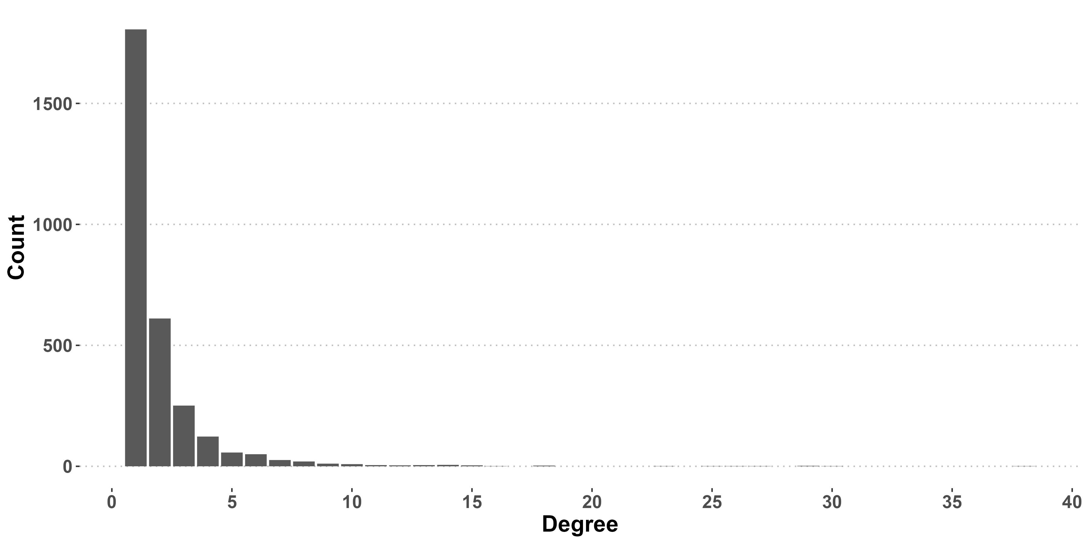
Figure F.1: Histogram of the baseline preferential attachment random network degree’s distribution. $n=3000$ nodes. The mean degree is $2$, and the maximal degree is $38$.

F.1.1 Illustration of the estimation bias

In this subsection, we report additional results of the simulation study shown in the main text.

Scenario (I) (Incorrect reporting of social connections).

Figure F.2 shows the relative bias (%) for additional estimands not displayed in the main text. The results were similar. The relative bias was larger for $\tau(c_{01},c_{00})$ and $\tau(c_{11},c_{10})$. When $\eta=0$ the bias is zero and increases with $\eta$ otherwise.

As discussed in Theorem 1, the bias from using a misspecified network structure results from selecting the wrong units and using invalid weights. Selecting the wrong units in our framework is equivalent to embedding units with the wrong exposure values. Figure F.3 shows the number of units with misclassified exposure values in the simulation. Clearly, the number of misclassified exposures increases with $\eta$, regardless of the exposure value.

The simulation validated Theorem 1 by illustrating that both Hajek and HT are unbiased whenever the network is correctly specified ($\eta=0$). However, HT had a larger empirical standard deviation (SD) than Hajek, possibly due to the stabilizing character of estimating $n$ when using Hajek (Särndal et al.,, 2003). Figure F.4 shows the empirical SD in nominal values. We can conclude that even though both HT and Hajek had a similar bias, Hajek had a lower SD.

To quantify the similarity of $\boldsymbol{A}^{\ast}$ and each of the misspecified networks, the Jaccard index was computed. Table F.1 displays the Jaccard index of $\boldsymbol{A}^{\ast}$ with each sampled network (by $\eta$). In the extreme ($\eta=0.25$), there were only about $15\%$ shared edges in the networks.

In the simulation, we sampled one incorrect network for each $\eta>0$ value. To illustrate that the results are robust for replications, Figure F.5 displays the results of additional $50$ replications in each we sampled different incorrect network. The bias across all replications is similar.

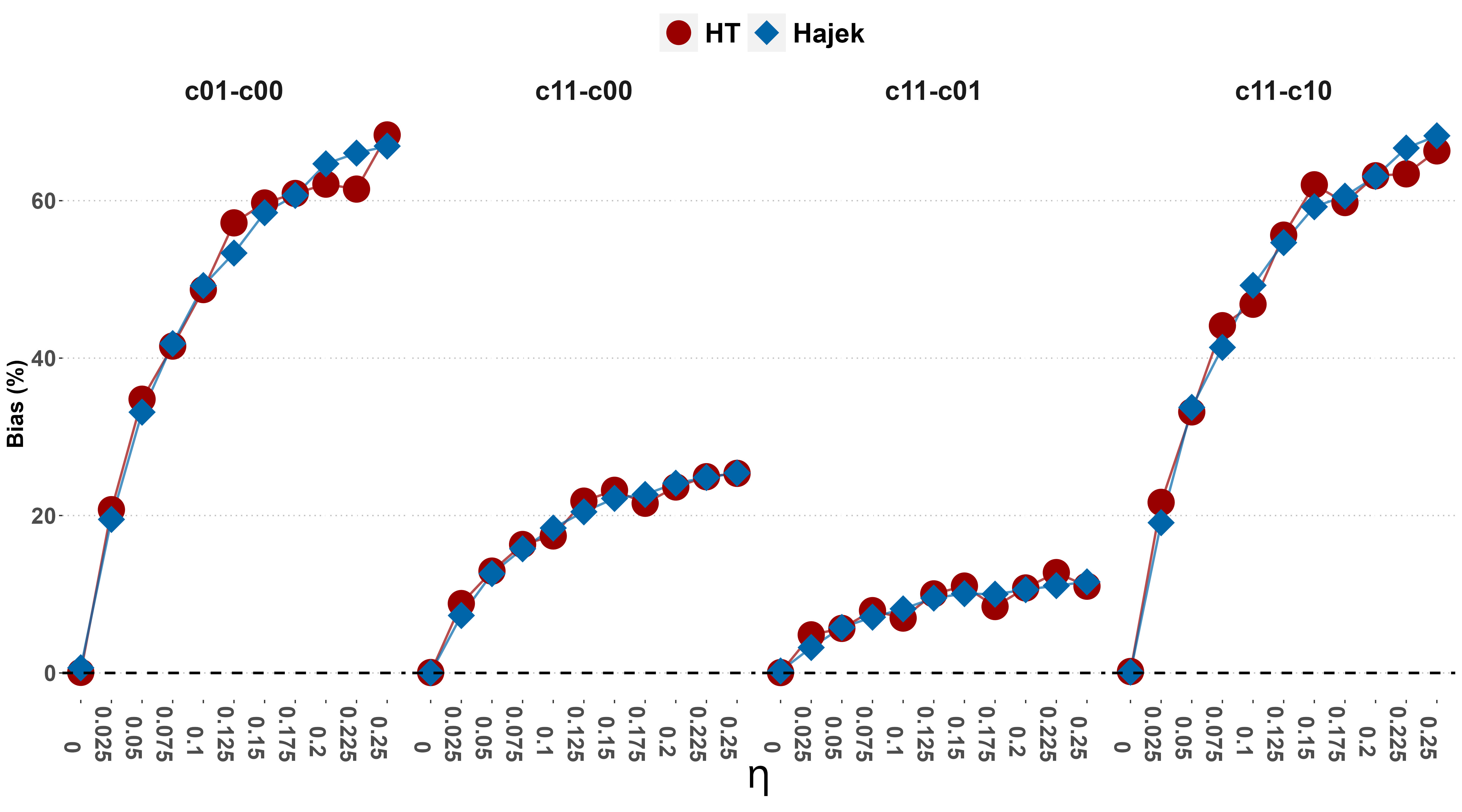
Figure F.2: Scenario (I). Additional relative bias (%) results from estimating $\tau(c_{01},c_{00}),\;\tau(c_{11},c_{00}),\;\tau(c_{11},c_{01}),\;\tau(c_{11},c_{10})$.

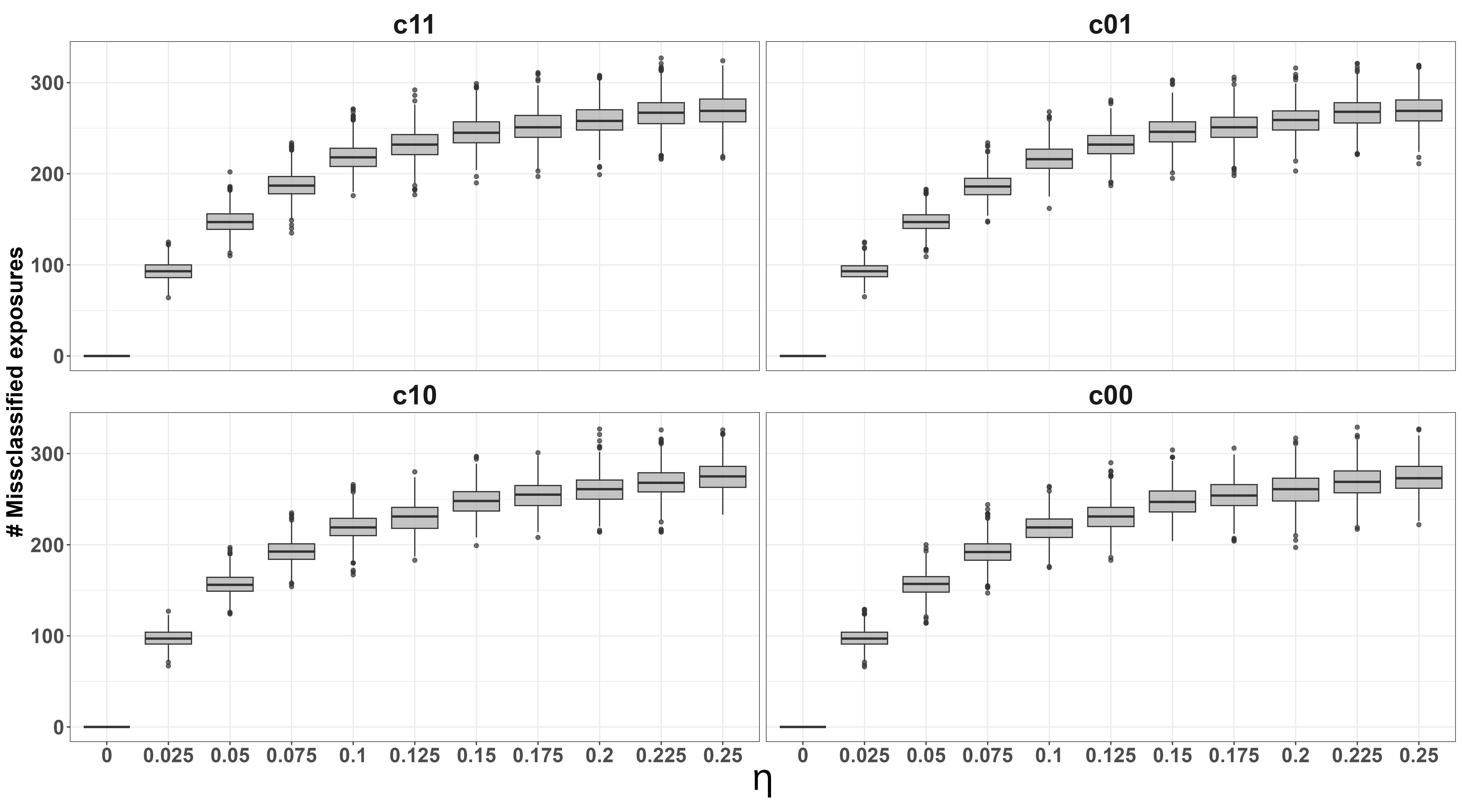
Figure F.3: Number of units with misclassified exposures by exposure value in Scenario (I).

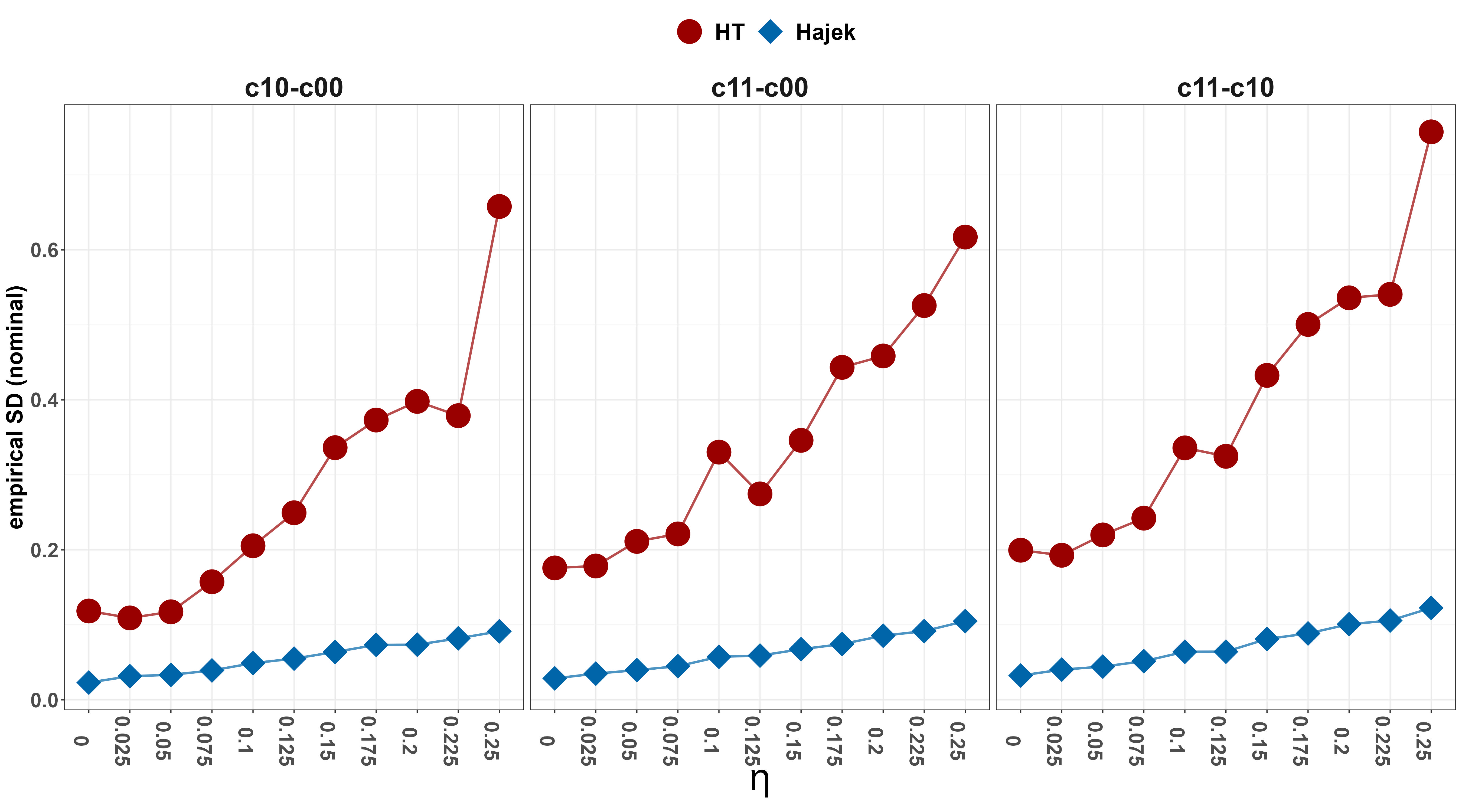
Figure F.4: Empirical standard deviation (SD) of HT and Hajek estimators in Scenario (I).

$\eta$	0	0.025	0.05	0.075	0.100	0.125	0.150	0.175	0.2	0.225	0.250
$J_{\boldsymbol{A}^{\ast},\boldsymbol{A}}$	1	0.709	0.55	0.433	0.352	0.305	0.256	0.231	0.2	0.174	0.157

Table F.1: Jaccard index of $\boldsymbol{A}^{\ast}$ and the misspecified networks in Scenario (I).

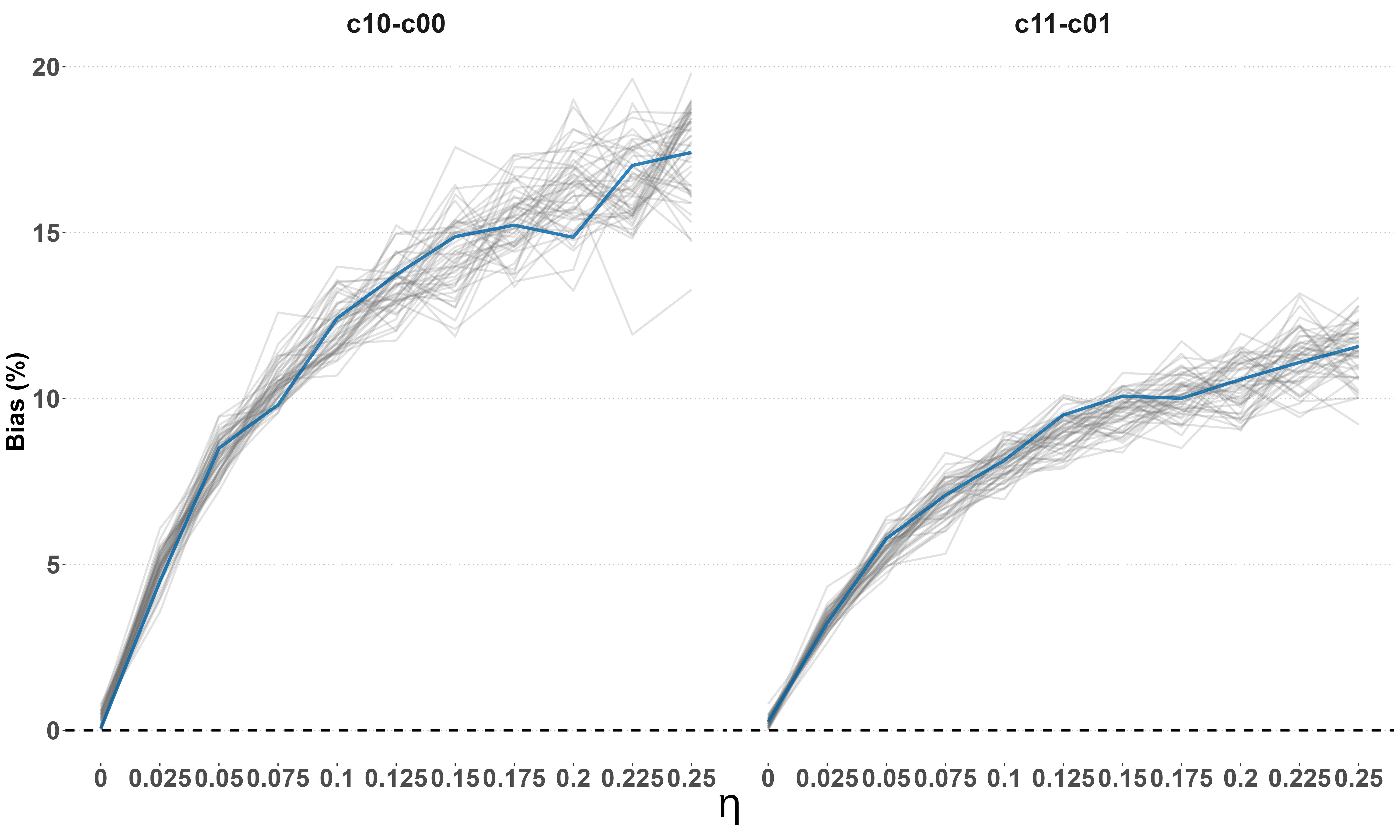
Figure F.5: Multiple replications of Scenario (I). The blue line represents the relative bias (%) of Hajek estimates shown in the main text, whereas each grey line results from the $50$ additional replication in which different networks are sampled for each $\eta>0$.

Scenario (II) (Censoring).

Here we also report additional results similar to the ones reported in the previous scenario. Table F.2 shows the proportion of units with more than $K=1,\dots,7$ neighbors, i.e., the proportion of units we censored some of their edges for each of the thresholds. For example, when $K=7$ only about $2.5\%$ units had censored edges, whereas when $K=1$ almost $40\%$ of units had censored edges. Figure F.6 shows relative bias for additional estimands not shown in the main text. The same picture holds. When the censoring threshold $K$ decreases, the bias increases, and the relative bias was larger. Notice that HT had a larger bias than Hajek when the censoring threshold $K$ decreased, probably due to the smaller effective sample size and the weights stability of Hajek. Figure F.7 displays the number of units with misclassified exposure values by censoring threshold $K$. Figure F.8 shows the empirical SD of HT and Hajek estimators in Scenario (II). Here also the SD of HT is uniformly higher than Hajek. However, the SD of HT decreases with $K$, i.e., when more censoring is present the variance is reduced. Table F.3 provides the Jaccard index of $\boldsymbol{A}^{\ast}$ and each of the censored networks. Similarly to Scenario (I), the index decreases with $K$. Figure F.9 shows that the results from additional $50$ replications of the simulations are almost identical for those reported.

$K$	1	2	3	4	5	6	7
$\Pr(d_{i}(\boldsymbol{A}^{\ast})>K)$	0.398	0.194	0.111	0.07	0.051	0.034	0.025

Table F.2: Edges empirical right-tail function in the PA network $\boldsymbol{A}^{\ast}$. $d_{i}(\boldsymbol{A}^{\ast})$ is the degree of unit $i$.

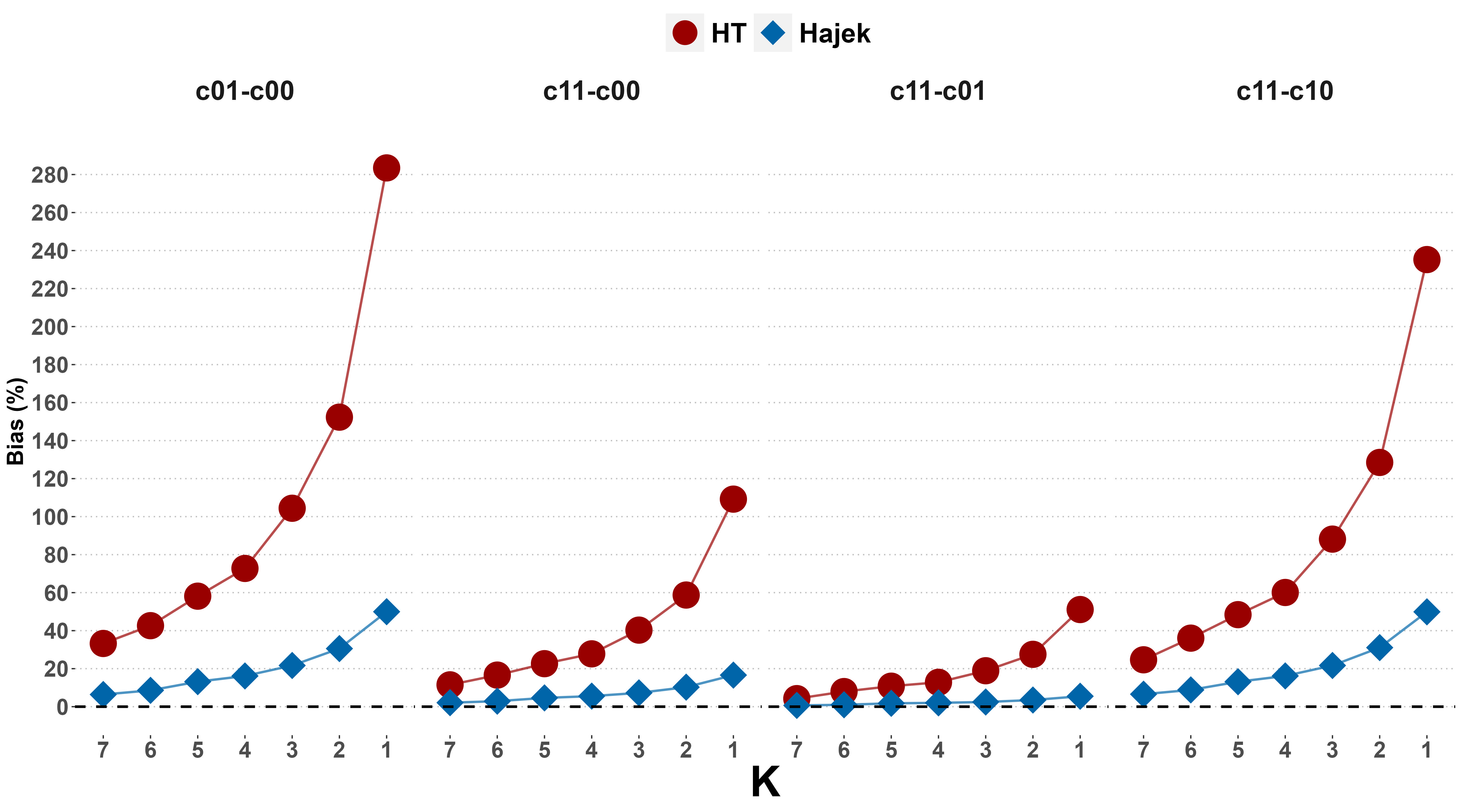
Figure F.6: Scenario (II). Additional absolute relative bias (%) results from estimating $\tau(c_{01},c_{00}),\;\tau(c_{11},c_{00}),\;\tau(c_{11},c_{01}),\;\tau(c_{11},c_{10})$.

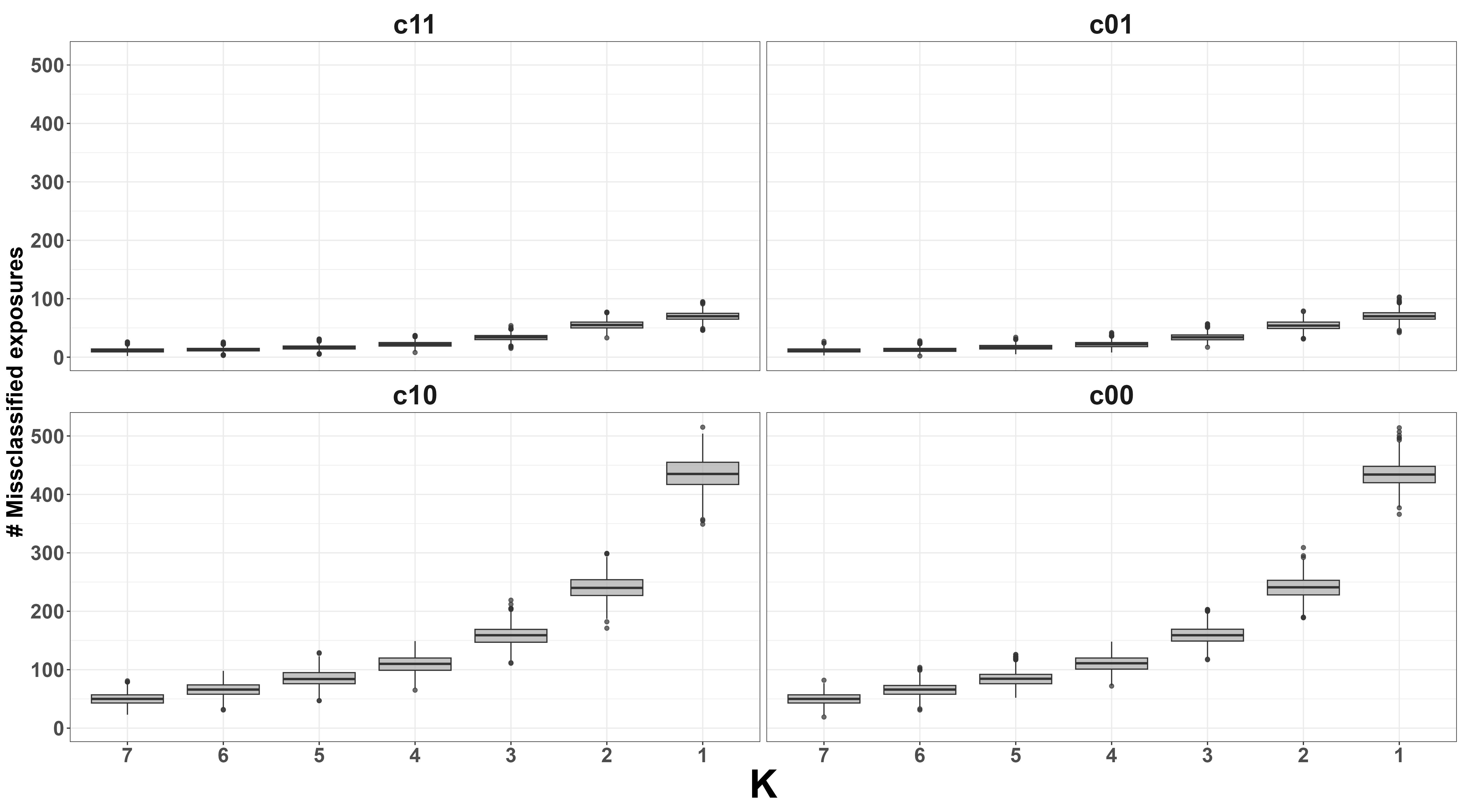
Figure F.7: Number of units with misclassified exposures by exposure value in Scenario (II).

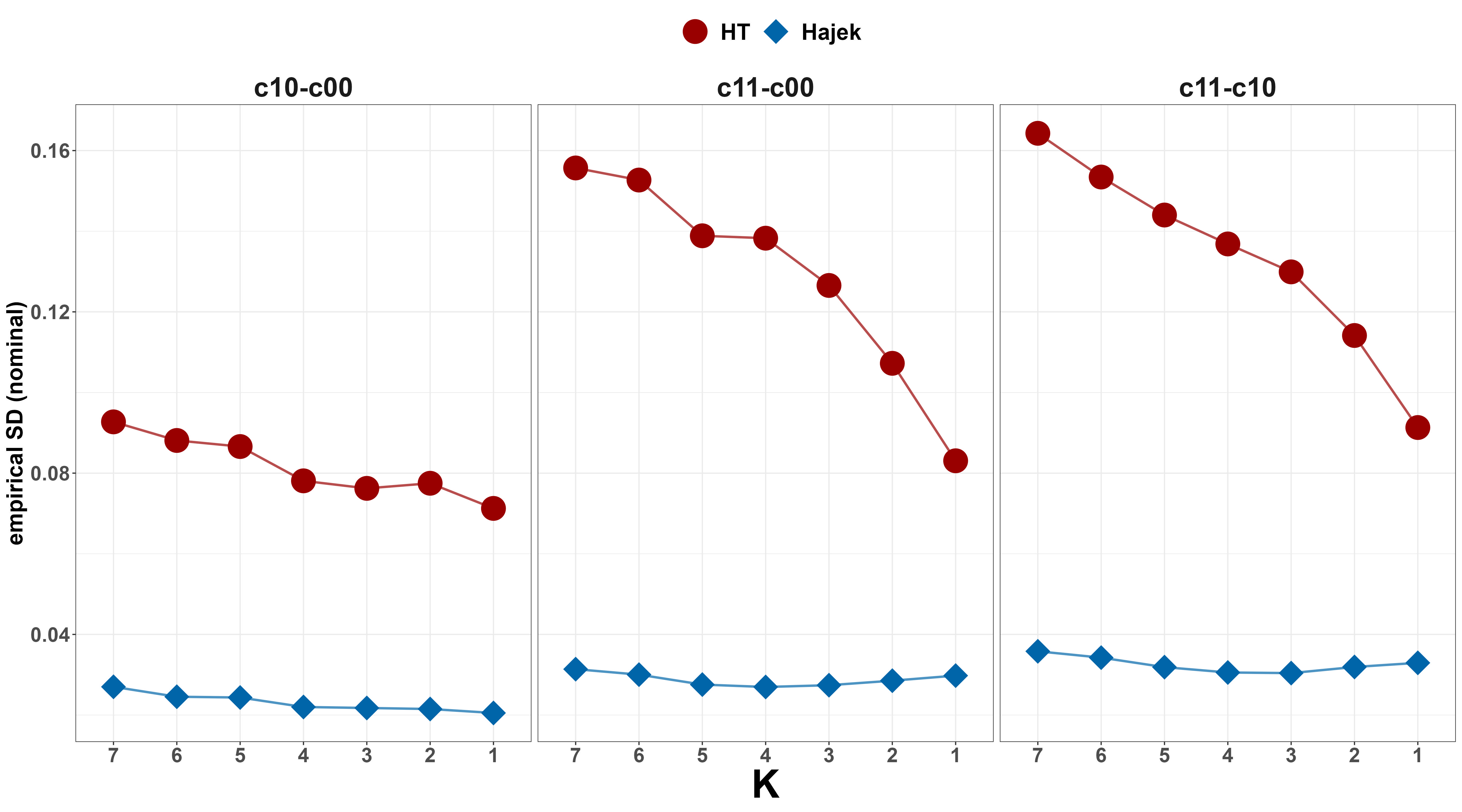
Figure F.8: Empirical standard deviation (SD) of HT and Hajek estimators in Scenario (II).

$K$	7	6	5	4	3	2	1
$J_{\boldsymbol{A}^{\ast},\boldsymbol{A}}$	0.865	0.836	0.794	0.736	0.644	0.499	0.258

Table F.3: Jaccard index of $\boldsymbol{A}^{\ast}$ and the censored networks in Scenario (II).

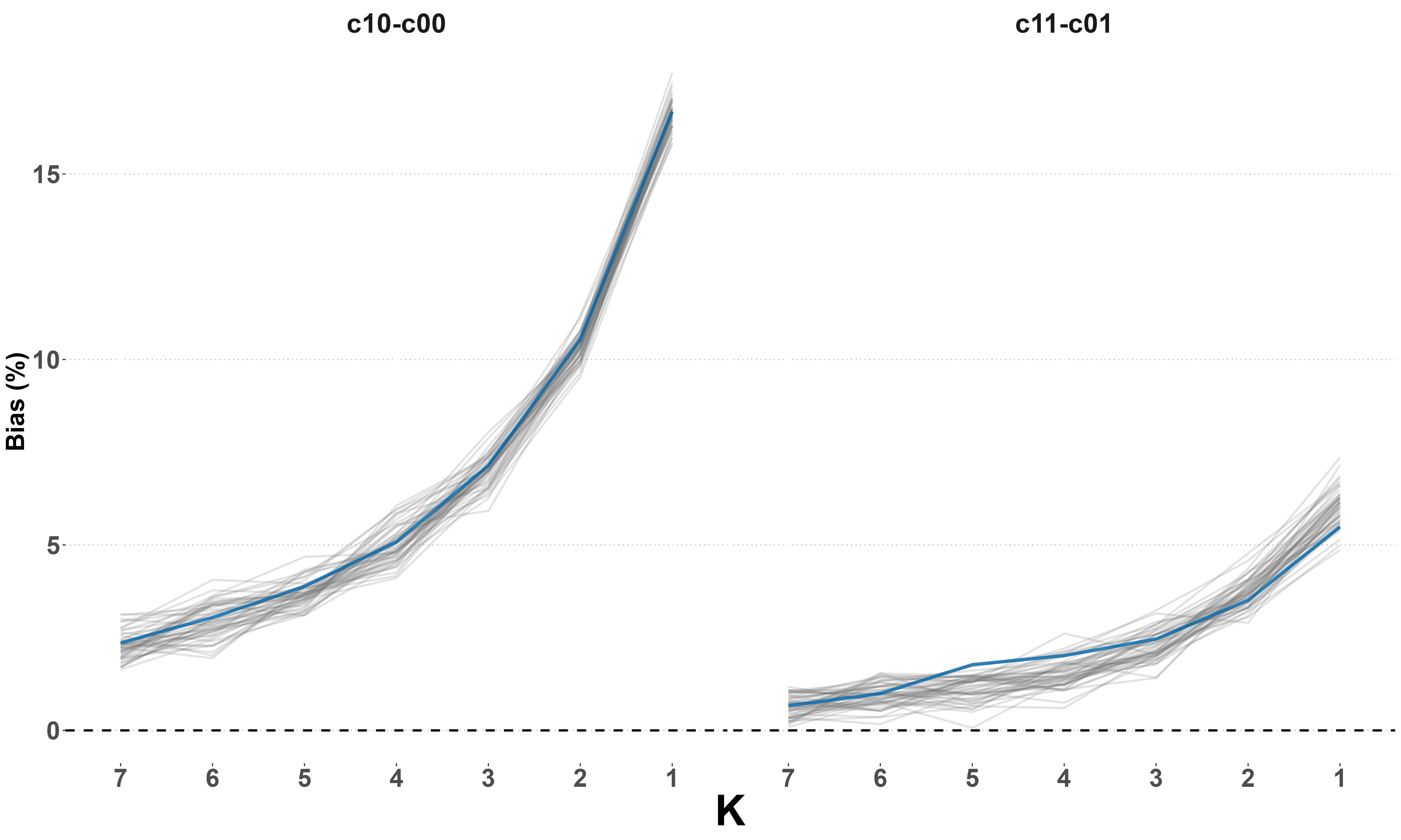
Figure F.9: Multiple replications of Scenario (II). The blue line represents the relative bias (%) of Hajek estimates shown in the main text, whereas each grey line results from the $50$ additional replication in which different networks are sampled for each $K$.

Scenario (III) (Cross-clusters contamination).

In the “varied” sizes scenario, cluster sizes were sampled from $U[3,7]$ distribution.

The relation between the estimated overall treatment effect $\tau(c_{11},c_{00})$ and common estimands in CRT is explained in online Appendix D. In addition, when the contamination probabilities $p_{v,v^{\prime}}$ are equal at the cluster level, i.e., not unit-specific, then the contaminated network can be modeled as a stochastic block model (SBM). Details are provided in online Appendix E.

F.1.2 Bias-variance tradeoff of the NMR estimators

Figure F.10 displays additional results of the bias-variance tradeoff simulation for $\tau(c_{01},c_{00})$ and $\tau(c_{11},c_{00})$. Similar results to those given in the main text appear there. Table F.4 shows the pairwise Jaccard indices of all the six networks used in the simulation.

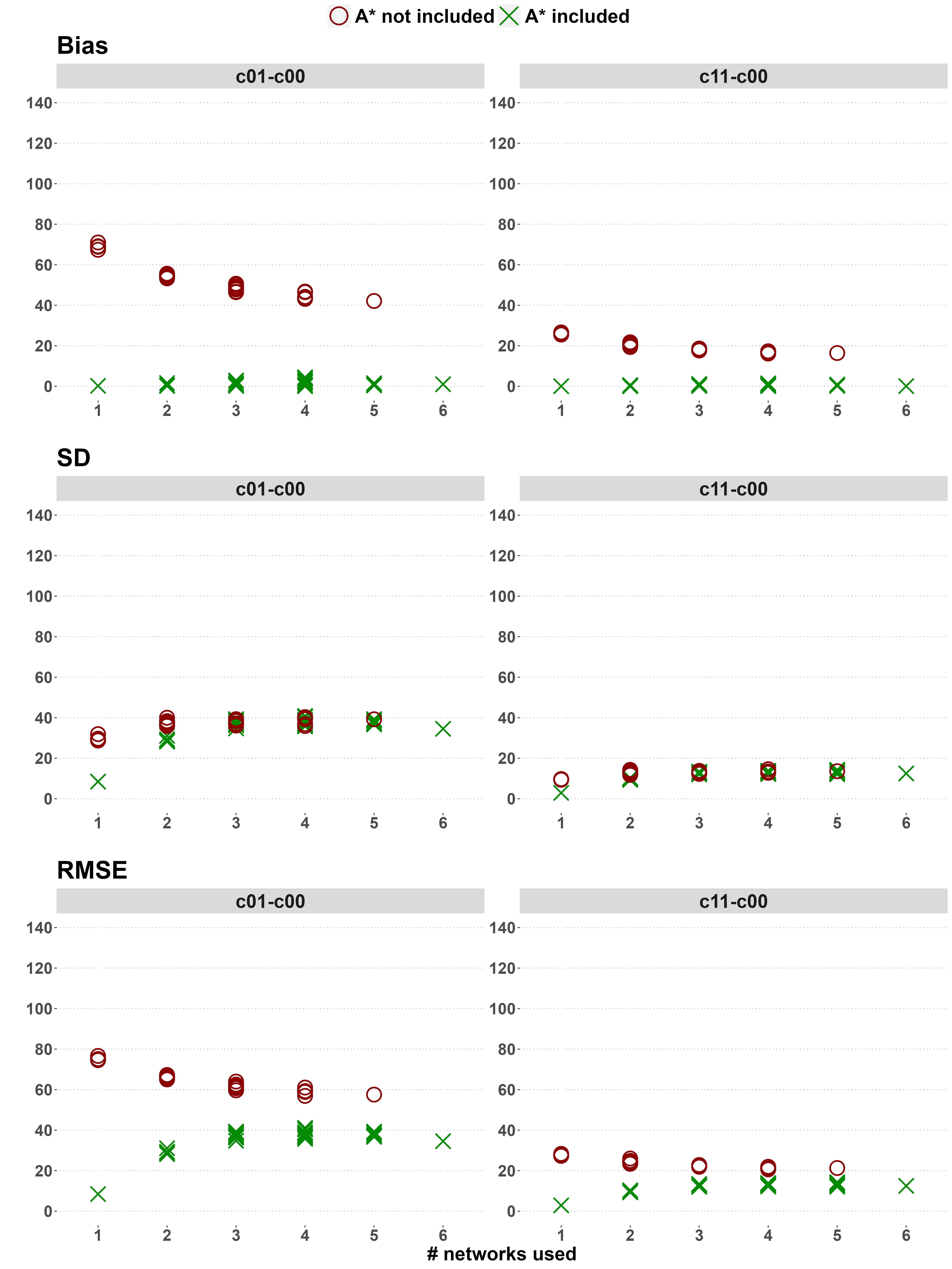
Figure F.10: Bias-variance tradeoff of the NMR estimator. Results presented are the bias, SD, and RMSE estimates (all reported in % relative to the true causal effects $\tau(c_{01},c_{00})$ and $\tau(c_{11},c_{00})$ for ease of presentation) of the Hajek NMR estimator.

	$\boldsymbol{A}^{\ast}$	$\boldsymbol{A}^{a}$	$\boldsymbol{A}^{b}$	$\boldsymbol{A}^{c}$	$\boldsymbol{A}^{d}$	$\boldsymbol{A}^{e}$
$\boldsymbol{A}^{\ast}$	1
$\boldsymbol{A}^{a}$	0.156	1
$\boldsymbol{A}^{b}$	0.155	0.066	1
$\boldsymbol{A}^{c}$	0.159	0.067	0.066	1
$\boldsymbol{A}^{d}$	0.157	0.067	0.068	0.068	1
$\boldsymbol{A}^{e}$	0.157	0.067	0.066	0.068	0.068	1

Table F.4: Jaccard index of the networks used in the simulations of the NMR bias-variance tradeoff.

F.1.3 Conservative variance estimators

We illustrate the conservative property of the NMR variance estimators proposed in online Appendix C in a small simulation study. In the same setup of the NMR bias-variance tradeoff simulation, we took all scenarios in which $\mathcal{A}$ contained the true networks $\boldsymbol{A}^{\ast}$ and compared the estimated conservative SE to the empirical SD. Figure F.11 displays the mean SE/SD ratio of $\tau(c_{01},c_{00})$ across the $1000$ iterations performed. Since all mean values are above one, we can surmise that the conservativeness property of the variance estimator holds. Nevertheless, it seems like the variance estimator is more conservative for Hajek than HT NMR estimators.

Figure F.11: Conservative NMR variance estimator. Values are the mean of $\tau(c_{01},c_{00})$ estimated SE/SD.

F.2 Data analyses

F.2.1 Social network field experiment

In our analysis of the data, we performed the same data pre-processing conducted by Paluck et al., (2016). The open-source replicability package provided by Paluck et al., (2016) can be found at https://www.icpsr.umich.edu/web/ICPSR/studies/37070. Table F.5 is an extended version of the results displayed in the main text. It contains the estimation of two more estimands ($\tau(c_{011},c_{000}),\;\tau(c_{111},c_{000})$) using more networks combinations. For example, we also use the NMR with both the ST networks (measured at the two time periods) simultaneously.

	$\tau(c_{001},c_{000})$		$\tau(c_{011},c_{000})$		$\tau(c_{101},c_{000})$		$\tau(c_{111},c_{000})$
Networks	HT	Hajek	HT	Hajek	HT	Hajek	HT	Hajek
ST-pre	0.061 (0.217)	0.146 (0.164)	0.162 (0.353)	0.122 (0.274)	0.096 (0.272)	0.271 (0.19)	0.369 (0.53)	0.272 (0.377)
BF-pre	0.084 (0.254)	0.123 (0.195)	0.068 (0.349)	0.162 (0.243)	0.169 (0.361)	0.265 (0.254)	0.143 (0.504)	0.292 (0.323)
ST-pre & BF-pre	0.051 (0.198)	0.134 (0.151)	0.11 (0.449)	0.135 (0.321)	0.079 (0.247)	0.261 (0.175)	0.224 (0.627)	0.258 (0.419)
ST-post	0.06 (0.214)	0.131 (0.164)	0.137 (0.38)	0.13 (0.282)	0.116 (0.298)	0.252 (0.212)	0.251 (0.513)	0.246 (0.355)
BF-post	0.09 (0.262)	0.135 (0.2)	0.039 (0.268)	0.09 (0.194)	0.17 (0.362)	0.258 (0.256)	0.134 (0.497)	0.297 (0.317)
ST-pre & ST-post	0.037 (0.17)	0.139 (0.13)	0.231 (0.483)	0.133 (0.37)	0.071 (0.233)	0.296 (0.161)	0.469 (0.662)	0.25 (0.493)
BF-pre & BF-post	0.077 (0.244)	0.124 (0.187)	0.037 (0.271)	0.063 (0.2)	0.15 (0.339)	0.258 (0.24)	0.154 (0.549)	0.303 (0.35)
ALL	0.04 (0.177)	0.178 (0.131)	0.067 (0.397)	0.051 (0.29)	0.046 (0.19)	0.227 (0.137)	0.266 (0.802)	0.226 (0.528)

Table F.5: Extended results of the social network field experiment analysis. Results are reported as point estimates (SE). Estimation is performed using the NMR HT and Hajek estimators.

Table F.6 shows the Jaccard index of the four available networks. Clearly, networks derived from the same questions are more similar than those from different questions, e.g., the similarity of ST and ST-2 is $27.5\%$ whereas those of ST and BF is $21.1\%$.

	ST-pre	ST-post	BF-pre	BF-post
ST-pre	1
ST-post	0.274	1
BF-pre	0.211	0.137	1
BF-post	0.137	0.200	0.244	1

Table F.6: Jaccard index of all the four available networks from Paluck et al., (2016).

F.2.2 Cluster-randomized trial

In the analysis of the data, we performed all the data pre-processing Venturo-Conerly et al., (2022) conducted. The data and all relevant information be found in the open-source replicability files provided by the authors https://osf.io/6qtjc/.

The baseline ($\theta=0$) estimates of causal effects were computed as we explained in online Appendix D. SE estimation was performed with Aronow and Middleton, (2013) proposed SE estimators for CRT settings.

References

- Aronow and Middleton, (2013) Aronow, P. M. and Middleton, J. A. (2013). A class of unbiased estimators of the average treatment effect in randomized experiments. Journal of Causal Inference, 1(1):135–154.
- Aronow and Samii, (2013) Aronow, P. M. and Samii, C. (2013). Conservative variance estimation for sampling designs with zero pairwise inclusion probabilities. Survey Methodology, 39(1):231–241.
- Aronow and Samii, (2017) Aronow, P. M. and Samii, C. (2017). Estimating average causal effects under general interference, with application to a social network experiment. The Annals of Applied Statistics, 11(4).
- Barabási and Albert, (1999) Barabási, A.-L. and Albert, R. (1999). Emergence of scaling in random networks. Science, 286(5439):509–512.
- Basse and Airoldi, (2018) Basse, G. W. and Airoldi, E. M. (2018). Limitations of design-based causal inference and A/B testing under arbitrary and network interference. Sociological Methodology, 48(1):136–151.
- Bhattacharya et al., (2020) Bhattacharya, R., Malinsky, D., and Shpitser, I. (2020). Causal inference under interference and network uncertainty. In Uncertainty in Artificial Intelligence, pages 1028–1038. PMLR.
- Borm et al., (2005) Borm, G. F., Melis, R. J. F., Teerenstra, S., and Peer, P. G. (2005). Pseudo cluster randomization: a treatment allocation method to minimize contamination and selection bias. Statistics in Medicine, 24(23):3535–3547.
- Boucher and Houndetoungan, (2022) Boucher, V. and Houndetoungan, E. A. (2022). Estimating peer effects using partial network data. Centre de recherche sur les risques les enjeux économiques et les politiques.
- Cai et al., (2015) Cai, J., Janvry, A. D., and Sadoulet, E. (2015). Social networks and the decision to insure. American Economic Journal: Applied Economics, 7(2):81–108.
- Chandrasekhar and Lewis, (2011) Chandrasekhar, A. and Lewis, R. (2011). Econometrics of sampled networks. Unpublished manuscript, MIT.[422].
- Cortez et al., (2022) Cortez, M., Eichhorn, M., and Yu, C. (2022). Staggered rollout designs enable causal inference under interference without network knowledge. In Advances in Neural Information Processing Systems.
- Cox, (1958) Cox, D. R. (1958). Planning of experiments. Wiley, New York.
- Ebel et al., (2002) Ebel, H., Davidsen, J., and Bornholdt, S. (2002). Dynamics of social networks. Complexity, 8(2):24–27.
- Egami, (2020) Egami, N. (2020). Spillover effects in the presence of unobserved networks. Political Analysis, 29(3):287–316.
- Forastiere et al., (2020) Forastiere, L., Airoldi, E. M., and Mealli, F. (2020). Identification and estimation of treatment and interference effects in observational studies on networks. Journal of the American Statistical Association, 116(534):901–918.
- Griffith, (2021) Griffith, A. (2021). Name your friends, but only five? the importance of censoring in peer effects estimates using social network data. Journal of Labor Economics.
- Halloran and Struchiner, (1991) Halloran, M. E. and Struchiner, C. J. (1991). Study designs for dependent happenings. Epidemiology, 2(5):331–338.
- Halloran and Struchiner, (1995) Halloran, M. E. and Struchiner, C. J. (1995). Causal inference in infectious diseases. Epidemiology, 6(2):142–151.
- Hardy et al., (2019) Hardy, M., Heath, R. M., Lee, W., and McCormick, T. H. (2019). Estimating spillovers using imprecisely measured networks. arXiv:1904.00136.
- Hartley and Ross, (1954) Hartley, H. O. and Ross, A. (1954). Unbiased ratio estimators. Nature, 174(4423):270–271.
- Hayek et al., (2022) Hayek, S., Shaham, G., Ben-Shlomo, Y., Kepten, E., Dagan, N., Nevo, D., Lipsitch, M., Reis, B. Y., Balicer, R. D., and Barda, N. (2022). Indirect protection of children from sars-cov-2 infection through parental vaccination. Science, 375(6585):1155–1159.
- Holland et al., (1983) Holland, P. W., Laskey, K. B., and Leinhardt, S. (1983). Stochastic blockmodels: First steps. Social Networks, 5(2):109–137.
- Hong and Raudenbush, (2006) Hong, G. and Raudenbush, S. W. (2006). Evaluating kindergarten retention policy. Journal of the American Statistical Association, 101(475):901–910.
- Hu et al., (2022) Hu, Y., Li, S., and Wager, S. (2022). Average direct and indirect causal effects under interference. Biometrika.
- Hubbard et al., (2016) Hubbard, A. E., Kherad-Pajouh, S., and van der Laan, M. J. (2016). Statistical inference for data adaptive target parameters. The International Journal of Biostatistics, 12(1):3–19.
- Hudgens and Halloran, (2008) Hudgens, M. G. and Halloran, M. E. (2008). Toward causal inference with interference. Journal of the American Statistical Association, 103(482):832–842.
- Leung, (2020) Leung, M. P. (2020). Treatment and spillover effects under network interference. The Review of Economics and Statistics, 102(2):368–380.
- Li et al., (2021) Li, W., Sussman, D. L., and Kolaczyk, E. D. (2021). Causal inference under network interference with noise. arXiv:2105.04518.
- Manski, (1993) Manski, C. F. (1993). Identification of endogenous social effects: The reflection problem. The Review of Economic Studies, 60(3):531.
- Manski, (2013) Manski, C. F. (2013). Identification of treatment response with social interactions. The Econometrics Journal, 16(1):S1–S23.
- Nagarajan et al., (2020) Nagarajan, K., Muniyandi, M., Palani, B., and Sellappan, S. (2020). Social network analysis methods for exploring SARS-CoV-2 contact tracing data. BMC Medical Research Methodology, 20(1).
- Ogburn et al., (2022) Ogburn, E. L., Sofrygin, O., Díaz, I., and van der Laan, M. J. (2022). Causal inference for social network data. Journal of the American Statistical Association, pages 1–46, https://doi.org/10.1080/01621459.2022.2131557.
- Paluck et al., (2016) Paluck, E. L., Shepherd, H., and Aronow, P. M. (2016). Changing climates of conflict: A social network experiment in 56 schools. Proceedings of the National Academy of Sciences, 113(3):566–571, https://www.pnas.org/doi/pdf/10.1073/pnas.1514483113.
- Rosenbaum, (2007) Rosenbaum, P. R. (2007). Interference between units in randomized experiments. Journal of the American Statistical Association, 102(477):191–200.
- Schaefer et al., (2012) Schaefer, D. R., Haas, S. A., and Bishop, N. J. (2012). A dynamic model of US adolescents’ smoking and friendship networks. American Journal of Public Health, 102(6):e12–e18.
- Särndal et al., (2003) Särndal, C.-E., Swensson, B., and Wretman, J. (2003). Model Assisted Survey Sampling (Springer Series in Statistics). Springer.
- Sävje, (2021) Sävje, F. (2021). Causal inference with misspecified exposure mappings. arXiv:2103.06471.
- Sävje et al., (2021) Sävje, F., Aronow, P. M., and Hudgens, M. G. (2021). Average treatment effects in the presence of unknown interference. The Annals of Statistics, 49(2).
- Tchetgen Tchetgen et al., (2020) Tchetgen Tchetgen, E. J., Fulcher, I. R., and Shpitser, I. (2020). Auto-g-computation of causal effects on a network. Journal of the American Statistical Association, 116(534):833–844.
- Tchetgen Tchetgen and VanderWeele, (2012) Tchetgen Tchetgen, E. J. and VanderWeele, T. J. (2012). On causal inference in the presence of interference. Statistical Methods in Medical Research, 21(1):55–75.
- Tortú et al., (2021) Tortú, C., Crimaldi, I., Mealli, F., and Forastiere, L. (2021). Causal effects with hidden treatment diffusion on observed or partially observed networks. arXiv:2109.07502.
- Tran and Zheleva, (2022) Tran, C. and Zheleva, E. (2022). Heterogeneous peer effects in the linear threshold model. arXiv:2201.11242.
- Ugander et al., (2013) Ugander, J., Karrer, B., Backstrom, L., and Kleinberg, J. (2013). Graph cluster randomization: Network exposure to multiple universes. In Proceedings of the 19th ACM SIGKDD international conference on Knowledge discovery and data mining, pages 329–337.
- VanderWeele, (2009) VanderWeele, T. J. (2009). Concerning the consistency assumption in causal inference. Epidemiology, 20(6):880–883.
- Venturo-Conerly et al., (2022) Venturo-Conerly, K. E., Osborn, T. L., Alemu, R., Roe, E., Rodriguez, M., Gan, J., Arango, S., Wasil, A., Wasanga, C., and Weisz, J. R. (2022). Single-session interventions for adolescent anxiety and depression symptoms in kenya: A cluster-randomized controlled trial. Behaviour Research and Therapy, 151:104040.
- Yu et al., (2022) Yu, C. L., Airoldi, E. M., Borgs, C., and Chayes, J. T. (2022). Estimating the total treatment effect in randomized experiments with unknown network structure. Proceedings of the National Academy of Sciences, 119(44).