Prediction-Correction Pedestrian Flow by Means of Minimum Flow Problem

Abstract.

We study a new variant of mathematical prediction-correction model for crowd motion. The prediction phase is handled by a transport equation where the vector field is computed via an eikonal equation $\displaystyle\|\nabla\varphi\|=f$, with a positive continuous function $\displaystyle f$ connected to the speed of the spontaneous travel. The correction phase is handled by a new version of the minimum flow problem. This model is flexible and can take into account different types of interactions between the agents, from gradient flow in Wassersetin space to granular type dynamics like in sandpile. Furthermore, different boundary conditions can be used, such as non-homogeneous Dirichlet (e.g., outings with different exit-cost penalty) and Neumann boundary conditions (e.g., entrances with different rates). Combining finite volume method for the transport equation and Chambolle-Pock’s primal dual algorithm for the eikonal equation and minimum flow problem, we present numerical simulations to demonstrate the behavior in different scenarios.

1. Introduction

Macroscopic model for a congested pedestrian flow involves treating the crowd as a whole and is applicable for large crowds. It was first introduced in [4] and developed in [23, 24]. In these models, the crowd behave similarly to a moving fluid in a spatio-temporal dynamic governed by a flow velocity vector field $\displaystyle U$. Thus the master equation of each macroscopic crowd flows model is the continuity equation:

$$\partial_{t}\rho+\operatorname{div}(\rho\>U)=0,$$ (1.1)

where $\displaystyle\rho=\rho(t,x)$ the density of the individuals, at time $\displaystyle t\geq 0$ and at the position $\displaystyle x\in\mathbb{R}^{N}$ ($\displaystyle N=2$), needs to accurate some admissible global distribution of the population. Though there is much speculation, discussion and experience to define appropriate choice of flow velocity vector field $\displaystyle U,$ there is no definitive universal choice to describe crowed motion in general. The main difficulties lies in the fact that while maintaining a suitable dynamic esteeming the admissible global distribution $\displaystyle\rho$, $\displaystyle U$ needs to manage both, the overall behavior of the crowd (for example of reaching an objective like exit, point of interest, avoidance of danger, etc.) and certain local behavior of pedestrians (pedestrian in a hurry, pedestrian who adapts their speed, pedestrian who avoids the crowd, pedestrian attracted by the crowd, etc).

Inspired by traffic flow models, many crowd motion models were performed essentially in one-dimensional space (c.f. [10, 23, 24]). In higher dimensions, Bellomo and Dogbe (c.f. [3, 15]) proposed coupling the continuity equation with

$$\partial_{t}U+(U\cdot\nabla_{x})U=F(\rho,U),$$

where the motion is governed by $\displaystyle F$, which has two parts: a relaxation term towards a definite speed, and a repulsive term to take into account that pedestrians tend to avoid high-density areas. A barrier method was proposed by Degond (cf. [13]) wherein the motion $\displaystyle F$ depends on a pressure that blows up when the density approaches a given congestion density. Piccoli and Tosin proposed another class of models in the framework of a time-evolving measure in [35, 36]. In their model the velocity of the pedestrian is composed by two terms: a desired velocity and an interaction velocity.

Roger Hughes proposed a completely different approach to describing pedestrian dynamics in [25], where a group of people wants to leave a domain with one or more exits/doors as quickly as possible. His main idea was to include some kind of saturation effects in the vector field. He considered $\displaystyle U=U[\rho]$ driven by the gradient of a potential $\displaystyle\Phi$ and weighted by a nonlinear mobility $\displaystyle f=f(\rho)$. More precisely

$$U=f(\rho)^{2}\nabla\Phi\quad\hbox{ and }\|\nabla\Phi\|=1/f(\rho),$$

where mobility includes saturation effects, i.e., degenerate behavior when approaching a given maximum density $\displaystyle\rho_{max}$ (assumed to be known); for instance one can take $\displaystyle f(\rho)=(\rho-\rho_{max})^{2}$ among others. See also [11] and [26] for further details.

To handle local behaviors of pedestrian, we go here with second order PDE for crowed motion to perform congestion phenomena which may appear if one consider velocity field $\displaystyle U$ looking out solely to the exists (doors). The main idea is to get in $\displaystyle U$ together a vector field $\displaystyle V$ with an overview looking out to the exit and some kind of patch $\displaystyle W$, a vector filed with a local view looking out to the allowable neighbor positions taking into account the local distribution of the pedestrian. To come out with $\displaystyle U$ through this perspective, we process by splitting the dynamic into two instantaneous phases: a first one, the so-called prediction phase, where the pedestrians move along the given vector filed $\displaystyle V,$ the so called spontaneous velocity field, and a second phase, the correction, which generates a patch $\displaystyle W$ that enables the pedestrian to move along allowable local paths to avoid congestion and maintain admissible global distribution of the pedestrian. A typical example of this point of view remains to be the constrained diffusion-transport equation which was performed in the pioneering work by B. Maury and al. (cf. [31]) through a predicting-correcting algorithm using a gradient flow in the Wasserstein space of probability measures. In this paper, we use a new manner to handle this perspective. In contrast with [31] where the author straighten up the density using some kind of projection in $\displaystyle\mathds{W}_{2}-$Wasserstein space in the correction phase, our approach is based on a new version of minimum flow problem. The approach is flexible and makes it possible to integrate several scenarios to deal with congestion. One can see also [27] where the approach is used to study similar dynamic in the case of two populations. In particular it allows to retrieve and compute otherwise the typical model of B. Maury, where the patch $\displaystyle W=W[\rho]$ is traced strictly in the so called congested/saturated regions as follow

$$W[\rho]=-\nabla p,\hbox{ with }p\geq 0\hbox{ and }p(\rho-1)=0.$$ (1.2)

Here $\displaystyle\rho\equiv 1$ workouts the utmost distribution of the population in $\displaystyle\Omega.$ Therefore, via this approach, the proposed system reads

$$\left\{\begin{array}[]{ll}\displaystyle\frac{\partial\rho}{\partial t}+\operatorname{div}(\rho\>(V-\nabla p))=0\\ \\ p\geq 0,\>0\leq\rho\leq 1,\>p(\rho-1)=0.\end{array}\right.$$ (1.3)

Furthermore, the approach enables to built a new model based on granular dynamic like in sandpile, presuming that individuals behave like grains in the congested zones. In some sense, at the microscopic level, the individuals travel by accruing randomly to the crowed, being placed either upon a heretofore unoccupied position in the direction of the exit or else upon the top of the stack of the crowd. Moreover, the local movement of the individuals may be weighted by a given function $\displaystyle\mathsf{k}$ connected to the speed of the spontaneous local movement. In this case, we prove that the patch is given by

$$W[\rho]=-m\nabla p$$ (1.4)

with unknown $\displaystyle m$ and $\displaystyle p$ satisfying

$$m\geq 0,\>p\geq 0,\>|\nabla p|\leq\mathsf{k},\>p(\rho-1)\hbox{ and }m\>(|\nabla p|-\mathsf{k})=0.$$ (1.5)

Here $\displaystyle m\geq 0$ is Lagrange multiplayer associated with the additional constraint $\displaystyle|\nabla p|\leq\mathsf{k}.$ The approach enables also to handle and integrate different boundary conditions. Neumann boundary condition is connected to the crossing boundary amount, and Dirichlet is connected to the possibility of crossing some parts of the boundary with different charges.

After all, via this approach, we introduce a new model of granular type :

$$\left\{\begin{array}[]{ll}\displaystyle\frac{\partial\rho}{\partial t}+\operatorname{div}(\rho\>(V-m\nabla p))=0\\ \\ 0\leq\rho\leq 1,\>p\geq 0,\>|\nabla p|\leq\mathsf{k}\\ \\ p(\rho-1)=0,\>m(|\nabla p|-\mathsf{k})=0,\end{array}\right.$$ (1.6)

subject to mixed boundary conditions (not necessary homogeneous), to describe a crowd motion where the movement of the agent is of granular type like in sandpile. In this paper, we propose its numerical study based on a new manner to handle the predicting-correcting algorithm to build the patch $\displaystyle W$. Over and above the transport equation (1.1), we proceed using as well a new version of minimum flow problem for optimal assignation as a step in the process to find the right assignment of the pedestrian. Roughly speaking, in the correction step we put together tow nested optimization procedures: a computation of a minimum flow with gainful assignment towards a specific part of the boundary (towards the exit) for arbitrary target, and then a coming up with the right target among all admissible ones. We show how one can retrieve and compute otherwise the typical model of B.Maury et al., (c.f. [31]) that we call up above. Then, we focus on the new model based on granular dynamics-like for sandpile.

The theoretical study of (1.6) is a challenging problem, especially existence and uniqueness questions, that we’ll treat likely in forthcoming works. Recall that, the case where the PDE is of diffusive type like in (1.3), the model is very employed to describe the behavior of population subject to global behavior governed by a vector field $\displaystyle V$ and a local one governed by the patch $\displaystyle W[\rho]$ (c.f. [31, 32, 33, 34] and the references therein). The uniqueness of a solution is a hard issue for these kind of problems that was treated recently by the second author in [28] (see also [14, 12]).

Organization of the paper.

This paper is organized as follows. In Section-2 we present our model, we give the details of each of its steps and we discuss two peculiar related PDEs to this model as well as some duality results on which our algorithm reposes. In Section-3, we show how to discretize the model. Since the approximation of the continuity equation is more or less classical, the novelty will be the use of a primal-dual method to solve the Beckmann-like problem. More particularly, this is given in Algorithm-3. In Section-4 we given several examples to illustrate our approach and we compare with some related works. Finally, we recall some tools and give some technical proofs in the Appendix.

2. The model

We consider an exit scenario, where $\displaystyle\Omega\subset\mathbb{R}^{N}$ ($\displaystyle N=2$) is a bounded open set with regular boundary $\displaystyle\displaystyle\partial\Omega=\Gamma_{N}\cup\Gamma_{D}.$ The set $\displaystyle\Omega$ represents the region where the crowd is moving, $\displaystyle\Gamma_{N}$ represents the (impenetrable) walls and $\displaystyle\Gamma_{D}$ the exits/doors.

2.1. Minimum flow problem

The key idea concerning the minimum flow problem goes back to Beckmann [2]. It consists in finding the optimal traffic flow field $\displaystyle\Phi$ between the two distributions given by $\displaystyle\mu_{1}$ and $\displaystyle\mu_{2}.$ That is to find the vector field $\displaystyle\Phi$ which satisfies the divergence equation

$$-\operatorname{div}(\Phi)=\mu_{1}-\mu_{2}\hbox{ in }\overline{\Omega},$$ (2.7)

and minimize a total cost of the traffic $\displaystyle\int F(x,\Phi(x))\>\mathrm{d}x,$ where $\displaystyle F\>:\>\Omega\times\mathbb{R}^{N}\to\mathbb{R}^{+}$ is a given function assumed to be at least continuous and convex with respect to the second variable. The equation (2.7) needs to be understood in the sense of $\displaystyle\mathcal{D}^{\prime}(\overline{\Omega}).$ In particular, the equation assigns a fixed normal trace to $\displaystyle\Phi$ on $\displaystyle\partial\Omega$ which is connected to the formal values of $\displaystyle\mu_{1}-\mu_{2}$ on $\displaystyle\partial\Omega.$

Here, we use a new variant to handle the pedestrian flow and carried out the patch $\displaystyle W$ for the spontaneous velocity field when the pedestrian is hindered by the other one. Indeed, we work with a modified traffic cost which handles some kind of gainful assignment towards a specific part of the boundary $\displaystyle\Gamma_{D}.$ More precisely, we consider the following momentum cost of the traffic

$$\mathcal{M}(\Phi):=\int_{\Omega}F(x,\Phi(x))\>\mathrm{d}x-\int_{\Gamma_{D}}g(x)\>\Phi\cdot\bm{\nu}\>\mathrm{d}x,$$

where $\displaystyle\Phi\cdot\bm{\nu}$ denotes the normal trace of $\displaystyle\Phi$ and $\displaystyle g$ patterns a given gainful charge for the assignment towards $\displaystyle\Gamma_{D}.$ Of course, for the optimization problem we have in mind we need to keep unrestricted the normal trace of $\displaystyle\Phi$ on $\displaystyle\Gamma_{D}$. Thus, the balance equation (2.7) turns into

$$-\operatorname{div}(\Phi)=\mu_{1}-\mu_{2}\hbox{ in }\mathcal{D}^{\prime}(\overline{\Omega}\setminus\Gamma_{D}).$$ (2.8)

See here, that the normal trace of $\displaystyle\Phi$ on the odd part $\displaystyle\Gamma_{N}$ remains to be given by $\displaystyle\mu_{1}-\mu_{2}$ on $\displaystyle\Gamma_{N}.$ For instance, working with $\displaystyle\mu_{1}$ and $\displaystyle\mu_{2}$ supported in $\displaystyle\Omega,$ we keep unrestricted the normal trace of $\displaystyle\Phi$ on $\displaystyle\Gamma_{D}$ but assigned it to $\displaystyle 0$ on $\displaystyle\Gamma_{N}.$

This being said, we consider the transportation cost associated with given densities $\displaystyle\mu_{1}$ and $\displaystyle\mu_{2}$ to be

$$\begin{array}[]{l}\inf_{\Phi}\Big{\{}\int_{\Omega}F(x,\Phi(x))\>\mathrm{d}x-\int_{\Gamma_{D}}g(x)\>\Phi\cdot\bm{\nu}\>\mathrm{d}x\>:\>\>-\operatorname{div}(\Phi)=\mu_{1}-\mu_{2}\hbox{ in }\mathcal{D}^{\prime}(\overline{\Omega}\setminus\Gamma_{D})\Big{\}}.\end{array}$$ (2.9)

Actually, for any arbitrary distributions $\displaystyle\mu_{1}$ and $\displaystyle\mu_{2},$ the optimization problem (2.9) aims to minimize both the transportation between $\displaystyle\mu_{1}$ and $\displaystyle\mu_{2},$ in $\displaystyle\Omega$ and towards $\displaystyle\Gamma_{D},$ by means of the cost function $\displaystyle F$ in $\displaystyle\Omega$, as well as the transportation towards the boundary $\displaystyle\Gamma_{D}$ paying the gainful charge $\displaystyle g(x)$ for each target position $\displaystyle x\in\Gamma_{D},$ respectively. Moreover, the new formulation enables to handle as well a provided incoming (or outgoing) flux on the remaining part $\displaystyle\Gamma_{N}.$

Notice here, that one needs to be careful with the notion of trace of $\displaystyle\Phi$ on the boundary since it is not well defined for all $\displaystyle\Phi$. One needs to be careful here with the notion of trace of $\displaystyle\Phi$ on the boundary since it is not well defined for all $\displaystyle\Phi$. However, working in

$$H_{\mathrm{div}}:=\Big{\{}\Phi\in L^{2}(\Omega):\leavevmode\nobreak\ \operatorname{div}(\Phi)\in L^{2}(\Omega)\Big{\}},$$

enables us to define $\displaystyle\Phi\cdot\bm{\nu}$ on $\displaystyle\Gamma_{D}$ in the right sense. Indeed, let $\displaystyle\gamma_{0}:H^{1}(\Omega)\to L^{2}(\Gamma)$ be the linear and continuous mapping satisfying $\displaystyle\gamma_{0}(u)=u_{|\Gamma}$ for all $\displaystyle u\in C(\overline{\Omega})$, where $\displaystyle\Gamma=\partial\Omega.$ Then, defining $\displaystyle H^{1/2}(\Gamma)=\gamma_{0}(H^{1}(\overline{\Omega}))$ and $\displaystyle H^{-1/2}(\Gamma)$ its dual, there exists a continuous trace operator $\displaystyle\gamma_{\textbf{n}}:H_{\mathrm{div}}(\Omega)\to H^{-1/2}(\Gamma)$ such that $\displaystyle\gamma_{\bm{\nu}}(\Phi)=\Phi\cdot\bm{\nu}$ for any $\displaystyle\Phi\in\mathcal{D}(\overline{\Omega})^{N}$. Thanks to Gauss’s Theorem, we have

$$\langle\gamma_{\bm{\nu}}(\Phi),\gamma_{0}(u)\rangle_{H^{-1/2},H^{1/2}}=\int_{\Omega}\Phi\cdot\nabla u\>\mathrm{d}x+\int_{\Omega}u\>\operatorname{div}(\Phi)\>\mathrm{d}x\>\>\text{ for all }\>\>u\in H^{1}(\Omega),\Phi\in H_{\mathrm{div}}(\Omega).$$

To simplify the presentation, we denote $\displaystyle\Phi\cdot\bm{\nu}:=\gamma_{\bm{\nu}}(\Phi),$ and moreover

$$\int_{\Gamma_{D}}g(x)\>\Phi\cdot\bm{\nu}\>\mathrm{d}x:=\langle\gamma_{\bm{\nu}}(\Phi),\tilde{g}\rangle_{H^{-1/2},H^{1/2}},$$

where $\displaystyle\tilde{g}\chi_{\Gamma_{D}}=g$ for $\displaystyle\tilde{g}\in H^{1/2}.$ Yet, one needs to assume that such $\displaystyle\tilde{g}$ exists (see the assumptions in Section 2.3).

Before ending this section, let us recall that a similar problem to (2.9) appears in [19] in the study of Hamilton-Jacobi equation (see also [21] and [20]). It appears also on a different form in the study of some Sobolev regularity for degenerate elliptic PDEs in [38]. Indeed, to avoid technicalities related to the normal trace of the flux on the boundary, it is possible to rewrite (2.9) as follows

$$\begin{array}[]{c}\inf_{\Phi,\upsilon}\left\{\int_{\Omega}F(x,\Phi(x))\>\mathrm{d}x-\int_{\Gamma_{D}}g(x)\>\upsilon(x)\>\mathrm{d}x\>:\>\>-\operatorname{div}(\Phi)=\mu_{1}-\mu_{2}\hbox{ in }\mathcal{D}^{\prime}(\overline{\Omega}\setminus\Gamma_{D})\right.\\ \\ \hbox{ and }\Phi\cdot\bm{\nu}=\upsilon\hbox{ on }\Gamma_{D}\Big{\}}.\end{array}$$ (2.10)

Remark 2.1.

Taking non-homogeneous boundary data $\displaystyle g$ and $\displaystyle\eta$ enables the treatment of congestion crowd motion in an urban area with many issues : incoming issues included in $\displaystyle\Gamma_{N}$ with supply rate given by $\displaystyle\eta$ and outgoing issues in $\displaystyle\Gamma_{D}$ with some kind of rate of return pictured by $\displaystyle g.$

In [38], the author studied some particular cases of (2.10) (like for instance the case where $\displaystyle\Gamma_{D}=\emptyset$ and also $\displaystyle\Gamma_{D}=\partial\Omega$). We notice also that in (2.9), the infimum in $\displaystyle\Phi$ is not reached in general and one looks in some situations (like for homogeneous $\displaystyle F$) for measure flow fields instead. This is related to the question of regularity of the transport density in mass transportation (see for instance the recent paper [17] and the references therein).

2.2. The algorithm

The main idea of prediction-correction algorithm is to split the dynamic into instantaneous successive processes : prediction then correction. The prediction step aims beforehand to move the population through a spontaneous velocity field. For this to happen, we use simply the transport equation (1.1) with $\displaystyle U=V,$ where $\displaystyle V$ derives from a potential governed by fast exit access trajectories. Afterward, as though the output of the prediction may be not feasible, we propose to catch up the upright deployment by applying the minimum flow assignment process (2.9) to the output of the prediction step; that we denote for the moment by $\displaystyle\tilde{\rho}$ and which should be a priori an $\displaystyle L^{\infty}$ function. Moreover, assuming that the dynamic is subject to some supply of population through incoming issues included in $\displaystyle\Gamma_{N},$ we propose to take

$$\mu_{1}=\tilde{\rho}\!\!\mathop{\hbox{ \vrule height=7.0pt,width=0.5pt,depth=0.0pt\vrule height=0.5pt,width=6.0pt,depth=0.0pt}}\nolimits\Omega+\eta\!\!\mathop{\hbox{ \vrule height=7.0pt,width=0.5pt,depth=0.0pt\vrule height=0.5pt,width=6.0pt,depth=0.0pt}}\nolimits\Gamma_{N},$$

where $\displaystyle\eta$ precisely designates the incoming supply through $\displaystyle\Gamma_{N}$. In this case, the constraint $\displaystyle-\operatorname{div}(\Phi)=\mu_{1}-\rho\hbox{ in }\mathcal{D}^{\prime}(\overline{\Omega}\setminus\Gamma_{D})$ is equivalent to say

$$-\operatorname{div}(\Phi)=\tilde{\rho}-\rho\quad\hbox{ in }\mathcal{D}^{\prime}(\Omega)\quad\hbox{ and }\quad\Phi\cdot\bm{\nu}=\eta\quad\hbox{ on }\Gamma_{N}.$$

The correction step we propose to construct $\displaystyle\rho$ requires to solve precisely the following optimization problem

$$\begin{array}[]{c}\inf_{(\Phi,\rho)}\left\{\int_{\Omega}F(x,\Phi(x))\>\mathrm{d}x-\int_{\Gamma_{D}}g(x)\>\Phi\cdot\bm{\nu}\>\mathrm{d}x\>:\>0\leq\rho\leq 1,\>-\operatorname{div}(\Phi)=\tilde{\rho}-\rho\hbox{ in }\mathcal{D}^{\prime}(\Omega)\right.\\ \\ \hskip 28.45274pt\hbox{ and }\Phi\cdot\bm{\nu}=\eta\hbox{ on }\Gamma_{N}\Big{\}}.\end{array}$$ (2.11)

The right space for each terms in (2.11) will be given in the following section. See that the output of the correction step provides as well the correction associated with $\displaystyle\tilde{\rho}$ and the suitable flow for the adjustment of the dynamic. We will see in the following section how the optimal flux $\displaystyle\Phi$ enables to carry out the patch $\displaystyle W$ for the spontaneous velocity field when this is necessary.

So, the algorithm may be written as follows : we consider $\displaystyle T>0$ a given time horizon. For a given time step $\displaystyle\tau>0,$ we consider a uniform partition of $\displaystyle[0,T]$ given by $\displaystyle t_{k}=k\tau,$ $\displaystyle k=0,\dotsc,n-1.$ Supposing that we know the density of the population $\displaystyle\rho_{k}$ at a given step $\displaystyle k,$ starting by $\displaystyle\rho_{0}.$ Then, we superimpose successively the following two steps :

• Prediction: In this predictive step, the density of population trends to grow up into

  $$\rho_{k+\frac{1}{2}}=\rho(t_{k+\frac{1}{2}}),$$

  where $\displaystyle\rho$ is the solution of the transport equation

  $$\partial_{t}\rho+\operatorname{div}(\rho\>V)=0\quad\hbox{ in }[t_{k},t_{k+\frac{1}{2}}[,$$ (2.12)

  with $\displaystyle\rho(t_{k})=\rho_{k}.$ Here, $\displaystyle V$ is spontaneous velocity field given by the geodesics toward the exit. To built its corresponding potential $\displaystyle\varphi$, we propose to solve the eikonal equation

  $$\left\{\begin{array}[]{ll}\|\nabla\varphi\|=f&\hbox{ in }\Omega,\\ \\ \varphi=0&\hbox{ on }\Gamma_{D},\end{array}\right.$$ (2.13)

  where $\displaystyle f$ is a given positive continuous function. Then, the spontaneous velocity field $\displaystyle V$ is given by $\displaystyle V:=-\nabla\varphi/\|\nabla\varphi\|.$ One sees here that the solution of (2.13) (in the sense of viscosity) gives the speedy path to the exit $\displaystyle\Gamma_{D}$. The potential $\displaystyle\varphi$ corresponds to the expected travel time to maneuver towards an exit. In particular, $\displaystyle\varphi$ is proportional to $\displaystyle f$ which may template space movement of traffic . As we will see, we can upgrade the spontaneous velocity field by taking $\displaystyle f$ depending on the density on real time (like in Hugue’s model).

• Correction: In general it is not expected that $\displaystyle\rho_{k+\frac{1}{2}}$ to be an allowable density of pedestrian, since this value may evolve outside the interval $\displaystyle[0,1].$ We propose then to proceed by the Beckmann-like process we introduced above to find the right apportionment of the pedestrian. That is to find $\displaystyle\rho_{k+1}$ using the optimization problem (2.11). More precisely, we propose to consider $\displaystyle\rho_{k+1}$ given by the following optimization problem

  $$\begin{array}[]{l}\operatorname*{arg\,min}_{\rho}\inf_{\Phi}\left\{\int_{\Omega}F(x,\Phi(x))\>\mathrm{d}x-\int_{\Gamma_{D}}g(x)\>\Phi\cdot\bm{\nu}\>\mathrm{d}x\>:\>\rho\in L^{\infty}(\Omega),\>0\leq\rho\leq 1,\>\right.\\ \\ \hskip 28.45274pt\Phi\in L^{2}(\Omega)^{N},\>-\tau\>\operatorname{div}(\Phi)=\rho_{k+1/2}-\rho\hbox{ in }\mathcal{D}^{\prime}(\Omega)\hbox{ and }\Phi\cdot\bm{\nu}=\eta\hbox{ on }\Gamma_{N}\Big{\}}.\end{array}$$ (2.14)

2.3. Related PDE

The application $\displaystyle F:\Omega\times\mathbb{R}^{N}\to[0,\infty)$ is assumed firstly to be continuous. As a primer practical case, one can consider the quadratic case, i.e.,

$$F(x,\xi)=\frac{1}{2}|\xi|^{2},\quad\hbox{ for any }x\in\Omega\hbox{ and }\xi\in\mathbb{R}^{N}.$$

More sophisticated situations arise by considering non-homogeneous $\displaystyle F$ that weights the cost according to space variables; like for instance

$$F(x,\xi)=\frac{c(x)}{s}\>|\xi|^{s},\quad\hbox{ for any }x\in\Omega\hbox{ and }\xi\in\mathbb{R}^{N},$$ (2.15)

with $\displaystyle 1<s<\infty.$ In particular, with the parameter $\displaystyle c$ one can scale the cost by focusing on and/or avoiding certain regions in space. A formal computation using duality à la Fenchel-Rockafellar (see e.g., [18]) implies that the infimum in (2.11) should coincide with

$$\inf_{p}\left\{\int p^{+}(x)\>\mathrm{d}x+\frac{1}{s^{\prime}}\int c(x)^{s^{\prime}-1}\>|\nabla p(x)|^{s^{\prime}}\>\mathrm{d}x-\int p(x)\>\tilde{\rho}(x)\>\mathrm{d}x\>:\>p\in W^{1,s^{\prime}}(\Omega),\ p=g\hbox{ on }\Gamma_{D}\right\},$$ (2.16)

where $\displaystyle s^{\prime}$ is the conjugate index of $\displaystyle s$, i.e., it satisfies $\displaystyle\frac{1}{s}+\frac{1}{s^{\prime}}=1$. Moreover, $\displaystyle p$ and $\displaystyle(\rho,\Phi)$ are solutions of both problems respectively, if and only if $\displaystyle(p,\rho,\Phi)$ is a solution of the following PDE

$$\left\{\begin{array}[]{ll}\left.\begin{array}[]{l}\rho-\operatorname{div}(\Phi)=\tilde{\rho}\\ \\ \rho\in\hbox{Sign}^{+}(p),\quad k\>\Phi=c^{s^{\prime}}\>|\nabla p|^{s^{\prime}-2}\nabla p\end{array}\right\}&\hbox{ in }\Omega,\\ \\ \Phi\cdot\bm{\nu}=\eta&\hbox{ on }\Gamma_{N},\\ \\ p=g&\hbox{ on }\Gamma_{D},\end{array}\right.$$ (2.17)

where $\displaystyle\hbox{Sign}^{+}$ is the maximal monotone graph given by

$$\operatorname{Sign}^{+}(r)=\left\{\begin{array}[]{ll}1&\text{ for }r>0\\ {[0,1]}&\text{ for }r=0\\ 0&\text{ for }r<0\end{array}\quad\text{ for }r\in\mathbb{R}.\right.$$

In other words, $\displaystyle\rho\in\operatorname{Sign}^{+}(p)$ is equivalent to says that $\displaystyle 0\leq\rho\leq 1$ and $\displaystyle p(1-\rho)=0$ in $\displaystyle\Omega.$ In this paper, we focus on the case where $\displaystyle s=1.$ For the treatment of the other cases, one can see [27] for more details. In particular, one sees that the quadratic case is closely connected to the system (1.3) which was proposed by B. Maury et al., [31] in the framework of gradient flows in the Wasserstein space of probability measures. As to the case (2.15), dynamical model which comes off following our approach is given by some kind of non linear $\displaystyle s^{\prime}-$Laplace equation

$$\left\{\begin{array}[]{ll}\displaystyle\frac{\partial\rho}{\partial t}+\operatorname{div}(\rho\>(V-W))=0,\quad k\>W=c^{s^{\prime}}\>|\nabla p|^{s^{\prime}-2}\nabla p\\ \\ p\geq 0,\>0\leq\rho\leq 1,\>p(\rho-1)=0\end{array}\right\}\quad\hbox{ in }(0,\infty)\times\Omega$$ (2.18)

subject to boundary conditions

$$\left\{\begin{array}[]{ll}\Phi\cdot\bm{\nu}=\eta&\hbox{ on }(0,\infty)\times\Gamma_{N},\\ \\ p=g&\hbox{ on }(0,\infty)\times\Gamma_{D}.\end{array}\right.$$ (2.19)

Notice that we use in (2.18), the fact that $\displaystyle\nabla p=\rho\>\nabla p,$ which is connected to $\displaystyle\rho\in\operatorname{Sign}^{+}(p)$.

As we said above, we focus here on the case where

$$F(x,\xi)=\mathsf{k}(x)\>|\xi|,\quad\hbox{ for any }(x,\xi)\in\Omega\times\mathbb{R}^{N},$$ (2.20)

where $\displaystyle 0\leq\mathsf{k}\in\mathcal{C}(\overline{\Omega}).$ This case is closely connected to granular dynamic like sandpile (see [16] and the references therein). In other words the individuals behaves like grains of sand (see [22] and also [29] for a stochastic microscopic description of the granular dynamic), in the congestion zone and not like a fluid as follows from the quadratic case. A peculiar choice may be the same function $\displaystyle f$

Moreover, in connection with gradient flow in the Wasserstein space, it is possible to connect our approach (in the case (2.20)) to the gradient flow in the Wasserstein space of probability measures equipped with $\displaystyle\mathds{W}_{1}.$ Indeed, in the case where $\displaystyle V\equiv 0,$ the link is well established at least in some particular case of nonlinearity connecting $\displaystyle\rho$ to $\displaystyle p$ (cf. [1]).

To treat the problem (2.11), we assume that the boundary data $\displaystyle g$ and $\displaystyle\eta$ are such that

• the exists $\displaystyle\tilde{g}\in W^{1,\infty}(\Omega),$ such that

  $$\nabla\tilde{g}(x)\in G(x):=\Big{\{}\xi\in\mathbb{R}^{N}\>:\>|\xi|\leq\mathsf{k}(x)\Big{\}},\hbox{ a.e. in }\Omega.$$ (2.21)

  and

  $$\tilde{g}=g\>\chi_{\Gamma_{D}}\quad\hbox{ on }\partial\Omega,$$ (2.22)

• there exists $\displaystyle 1<s<\infty$ such that

  $$\eta\in W^{-\frac{1}{s},s}(\Gamma_{N}).$$

Then, for any $\displaystyle\mu\in L^{s}(\Omega),$ we define

$$\mathcal{F}(\mu):=\Big{\{}\Phi\in L^{s}(\Omega)^{N}\>:\>-\operatorname{div}(\Phi)=\mu\hbox{ in }\Omega\hbox{ and }\Phi\cdot\bm{\nu}=\eta\hbox{ on }\Gamma_{N}\Big{\}}.$$

Remind here, that $\displaystyle-\operatorname{div}(\Phi)=\mu$ in $\displaystyle\Omega$ and $\displaystyle\Phi\cdot\bm{\nu}=\eta$ on $\displaystyle\Gamma_{N}$ needs to be understood in the sense that

$$\int_{\Omega}\Phi\cdot\nabla\xi\>\mathrm{d}x=\int_{\Omega}\mu\>\xi\>\mathrm{d}x+\int_{\Gamma_{N}}\eta\>\xi\>\mathrm{d}x,\quad\hbox{ for any }\xi\in W^{1,s^{\prime}}_{\Gamma_{D}}(\Omega).$$ (2.23)

We are interested into the interpretation in terms of PDE of the solution of the problem

$$\mathcal{N}(\tilde{\rho}):=\inf_{\Phi,\rho}\left\{\tau\>\int_{\Omega}\mathsf{k}(x)\>|\Phi(x)|\>\mathrm{d}x-\tau\>\int_{\Gamma_{D}}g\>\Phi\cdot\bm{\nu}\>\mathrm{d}x\>:\>\tau\>\Phi\in\mathcal{F}(\tilde{\rho}-\rho)\hbox{ and }\rho\in\mathcal{K}_{1}\right\},$$ (2.24)

where $\displaystyle 0\leq\tilde{\rho}\in L^{s}(\Omega)$ is fixed and $\displaystyle K_{1}$ is the set of admissible densities:

$$\mathcal{K}_{1}=\{\rho\in L^{\infty}(\Omega)\>:\>0\leq\rho\leq 1\hbox{ a.e. in }\Omega\}.$$

See that, all the terms in $\displaystyle\mathcal{N}(\tilde{\rho})$ are well defined. Indeed, since $\displaystyle\Phi\in L^{s}(\Omega)^{N}$ and $\displaystyle\nabla\cdot\Phi\in L^{s}(\Omega),$ the normal trace of $\displaystyle\Phi$ is well defined on $\displaystyle\Gamma_{D}$ and $\displaystyle\Gamma_{N}.$ Actually $\displaystyle\int_{\Gamma_{D}}g\>\Phi\cdot\bm{\nu}\>\mathrm{d}x$ and $\displaystyle\Phi\cdot\bm{\nu}=\eta\hbox{ on }\Gamma_{N}$ need to be understood, respectively, in the sense of

$$\langle\Phi\cdot\bm{\nu},\tilde{g}\rangle_{W^{-1/s,s}(\Gamma_{D}),W^{1-1/s^{\prime},s^{\prime}}(\Gamma)}$$

and

$$\int_{\Omega}\Phi\cdot\nabla\xi\>\mathrm{d}x+\int_{\Omega}\xi\>\nabla\cdot\Phi\>\mathrm{d}x=\langle\eta,\xi\rangle_{W^{-1/s,s}(\Gamma),W^{1-1/s^{\prime},s^{\prime}}(\Gamma)},\quad\hbox{ for any }\xi\in W^{1,s}_{\Gamma_{D}}(\Omega).$$

Our main result here is the following

Theorem 2.2.

For any $\displaystyle 0\leq\tilde{\rho}\in L^{s}(\Omega)$ , we have

$$\mathcal{N}(\tilde{\rho})=\max_{p\in\mathcal{G}_{\mathsf{k}}}\Big{\{}\int_{\Omega}\tilde{\rho}\>p\>\mathrm{d}x+\tau\>\int_{\Gamma_{N}}\eta\>p\>\mathrm{d}x-\int_{\Omega}p^{+}\>\mathrm{d}x\Big{\}}:=D_{g}^{\infty}(\tilde{\rho}),$$ (2.25)

where

$$\mathcal{G}_{\mathsf{k}}:=\Big{\{}z\in W^{1,\infty}(\Omega)\>:\>z=g\hbox{ on }\Gamma_{D}\hbox{ and }|\nabla z(x)|\leq\mathsf{k}(x)\hbox{ a.e. }x\in\Omega\Big{\}}.$$

Moreover,

$$\mathcal{N}(\tilde{\rho})=\min_{\rho\in\mathcal{K}_{1}}\inf_{\tau\Phi\in\mathcal{F}(\tilde{\rho}-\rho)}\left\{\tau\int_{\Omega}\mathsf{k}(x)\>|\Phi(x)|\>\mathrm{d}x-\tau\int_{\Gamma_{D}}g(x)\>\Phi\cdot\bm{\nu}\>\mathrm{d}x\right\},$$ (2.26)

and, if $\displaystyle\rho$ and $\displaystyle p$ are optimal solutions of both problems $\displaystyle\mathcal{N}(\tilde{\rho})$ and $\displaystyle D_{g}^{\infty}(\tilde{\rho})$ respectively, then $\displaystyle p\in\mathcal{G}_{\mathsf{k}}$, $\displaystyle\rho\in\mathcal{K}_{1},$ $\displaystyle\rho\in\hbox{Sign}^{+}(p),$ a.e. in $\displaystyle\Omega$ and

$$\int_{\Omega}(\tilde{\rho}-\rho)\>(p-\xi)\>\mathrm{d}x-\tau\>\int_{\Gamma_{N}}\eta\>(p-\xi)\>\mathrm{d}x\geq 0,\quad\hbox{ for any }\xi\in\mathcal{G}_{\mathsf{k}}.$$ (2.27)

Remark 2.3.

Thanks to Theorem 2.2, one sees that the condition (2.22) is a sufficient and necessary condition. It is more or less well known by now that this condition is equivalent to the fact that (see for instance [19])

$$g(x)-(y)\leq\min\left\{\int_{0}^{1}\mathsf{k}(\varphi(t))\>|\dot{\varphi}(t)|\>\mathrm{d}t\>:\>\varphi\in\textup{Lip}([0,1],\Omega),\>\varphi(0)=x,\>\varphi(1)=y\right\}.$$

To prove Theorem 2.2, we use Von Neumann-Fan minimax theorem that we remind below

Theorem (Von Neumann-Fan minimax theorem, see for instance [5]).

Let $\displaystyle X$ and $\displaystyle Y$ be Banach spaces. Let $\displaystyle C\subset X$ be nonempty and convex, and let $\displaystyle D\subset Y$ be nonempty, weakly compact and convex. Let $\displaystyle g\>:\>X\times Y\to\mathbb{R}$ be convex with respect to $\displaystyle x\in C$ and concave and upper-semicontinuous with respect to $\displaystyle y\in D,$ and weakly continuous in $\displaystyle y$ when restricted to $\displaystyle D.$ Then

$$\max_{y\in D}\inf_{x\in C}g(x,y)=\inf_{x\in C}\max_{y\in D}g(x,y).$$

To this aim, we use the following result which goes back to [19] in the case where $\displaystyle\eta\equiv 0.$ For completeness, a proof is given in Appendix-C.

Lemma 2.4.

We have

$$\begin{array}[]{l}\inf_{\tau\Phi\in\mathcal{F}(\tilde{\rho}-\rho)}\left\{\tau\int_{\Omega}\mathsf{k}(x)\>|\Phi(x)|\>\mathrm{d}x-\tau\int_{\Gamma_{D}}g(x)\>\Phi\cdot\bm{\nu}\>\mathrm{d}x\right\}\\ \\ \hskip 28.45274pt=\max_{p\in\mathcal{G}_{\mathsf{k}}}\left\{\int(\tilde{\rho}-\rho)\>p\>\mathrm{d}x-\tau\>\int_{\Gamma_{N}}p\>\eta\>\mathrm{d}x\right\}.\end{array}$$ (2.28)

Proof of Theorem 2.2.

Since $\displaystyle\tilde{\rho}-\rho\in L^{s}(\Omega)$ and $\displaystyle\eta\in W^{-\frac{1}{s},s}(\Gamma_{N})$, we know that $\displaystyle\mathcal{F}(\tilde{\rho}-\rho)\neq\emptyset$. Moreover, since

$$\mathcal{N}(\tilde{\rho})=\inf_{\rho\in\mathcal{K}_{1}}\inf_{\tau\Phi\in\mathcal{F}(\tilde{\rho}-\rho)}\left\{\tau\int_{\Omega}\mathsf{k}(x)\>|\Phi(x)|\>\mathrm{d}x-\tau\int_{\Gamma_{D}}g(x)\>\Phi\cdot\bm{\nu}\>\mathrm{d}x\right\},$$ (2.29)

by Lemma 2.4, we get

$$\mathcal{N}(\tilde{\rho})=\inf_{\rho\in\mathcal{K}_{1}}\max_{p\in\mathcal{G}_{\mathsf{k}}}\left\{\int(\tilde{\rho}-\rho)\>p\>\mathrm{d}x-\tau\>\int_{\Gamma_{N}}p\>\eta\>\mathrm{d}x\right\}.$$ (2.30)

Using Von Neumann-Fan minimax theorem as in [5], we deduce that

$$\displaystyle\mathcal{N}(\tilde{\rho}) \displaystyle= \displaystyle\max_{p\in\mathcal{G}_{\mathsf{k}}}\inf_{\rho\in\mathcal{K}_{1}}\left\{\int(\tilde{\rho}-\rho)\>p\>\mathrm{d}x-\tau\>\int_{\Gamma_{N}}p\>\eta\>\mathrm{d}x\right\}$$ (2.31)

$$\displaystyle= \displaystyle\max_{p\in\mathcal{G}_{\mathsf{k}}}\left\{\int\tilde{\rho}\>p\>\mathrm{d}x-\int p^{+}\>\mathrm{d}x-\tau\>\int_{\Gamma_{N}}p\>\eta\>\mathrm{d}x\right\}.$$ (2.33)

Taking

$$p=\operatorname*{arg\,max}_{p\in W^{1,\infty}(\Omega),\>p_{\mid\Gamma_{D}}=g}\left\{\int\tilde{\rho}\>p\>\mathrm{d}x-\int p^{+}\>\mathrm{d}x+\tau\>\int_{\Gamma_{N}}p\>\eta\>\mathrm{d}x\right\}$$

and $\displaystyle\rho=\hbox{Sign}_{0}^{+}(p)$ and using Lemma 2.4, we deduce the equivalence between the solutions of (2.28) and (2.17). Thus the result of the theorem.

∎

Remark 2.5.

1. It is known that the optimal flux in (2.26) is not reached for a Lebesgue vector valued function $\displaystyle\Phi.$ Indeed, since the structure of $\displaystyle F,$ one expects the optimal flux to be a Radon measure vector valued function $\displaystyle\Phi$. However, if this is true and if $\displaystyle(\rho,\Phi)$ and $\displaystyle p$ are solutions of both problems $\displaystyle\mathcal{N}(\tilde{\rho})$ and $\displaystyle D(\tilde{\rho})$ respectively, then $\displaystyle\rho\in\hbox{Sign}^{+}(p),$ a.e. in $\displaystyle\Omega,$ $\displaystyle\Phi\cdot\nabla p=\mathsf{k}\>|\Phi|$ in $\displaystyle\Omega$ and

   $$\tau\>\int_{\Omega}\Phi\cdot\nabla\xi\>\mathrm{d}x=\int_{\Omega}(\tilde{\rho}-\rho)\>\xi\leavevmode\nobreak\ \mathrm{d}x+\tau\>\int_{\Gamma_{N}}\eta\>\xi\>\mathrm{d}x,\quad\hbox{ for any }\xi\in W^{1,s^{\prime}}_{\Gamma_{D}}(\Omega).$$ (2.34)

   In general, one needs to be careful with the treatment of $\displaystyle\Phi\cdot\nabla p,$ since $\displaystyle\Phi$ is not regular in general. Here one needs, to use the notion of tangential gradient of $\displaystyle p$ (see e.g., [6]) to handle the related PDE.

2. In connection with Evans-Gangbo formulation, the corresponding PDE may be written as

   $$\left\{\begin{array}[]{ll}\displaystyle\tilde{\rho}-\tau\>\operatorname{div}(\rho\>W)=0,\quad W=m\>\nabla p\\ \\ m\geq 0,\>p\geq 0,\>0\leq\rho\leq 1,\>p(\rho-1)=0\\ \\ |\nabla p|\leq\mathsf{k},\>m(|\nabla p|-\mathsf{k})=0\end{array}\right\}\quad\hbox{ in }\Omega,$$ (2.35)

   subject to boundary condition

   $$\left\{\begin{array}[]{ll}\displaystyle\Phi\cdot\bm{\nu}=\eta&\hbox{ on }(0,\infty)\times\Gamma_{N},\\ \\ p=g&\hbox{ on }(0,\infty)\times\Gamma_{D}.\end{array}\right.$$ (2.36)

3. As a formal consequence of Theorem 2.2, under the assumptions (H1)-(H2), the algorithm in Section 2.2 turns out in solving successively two PDEs, a transport equation and a nonlinear second order equation. This enables also to establish a continuous model in terms of nonlinear PDE. This is summarized in the following items.

   1. The sequence $\displaystyle\rho_{1/2},\rho_{1},\dotsc,\rho_{k},\rho_{k+1/2},\rho_{k+1},\dotsc,\rho_{n}$ given by the algorithm in Section 2.2 is characterized by: for each $\displaystyle k=0,\dotsc,n-1,$ we have

      • Prediction: $\displaystyle\rho_{k+\frac{1}{2}}=\rho(t_{k+\frac{1}{2}}),$ where $\displaystyle\rho$ is the solution of the transport equation :

        $$\partial_{t}\rho+\operatorname{div}(\rho\>V)=0\quad\hbox{ in }[t_{k},t_{k+\frac{1}{2}}[,$$ (2.37)

        with $\displaystyle\rho(t_{k})=\rho_{k},$ $\displaystyle V$ is a given vector field. For instance $\displaystyle V=-\nabla\varphi/\|\nabla\varphi\|$ and $\displaystyle\varphi$ is the solution of the eikonal equation (2.13).

      • Correction: $\displaystyle\rho_{k+1}$ is a solution of the PDE

        $$\left\{\begin{array}[]{ll}\left.\begin{array}[]{l}\rho_{k+1}-\tau\>\operatorname{div}(\rho_{k+1}\>W)=\rho_{k+1/2},\quad W=m\>\nabla p_{k+1}\\ \\ m\geq 0,\>p_{k+1}\geq 0,\>0\leq\rho_{k+1}\leq 1,\>p_{k+1}(\rho_{k+1}-1)=0\\ \\ |\nabla p_{k+1}|\leq\mathsf{k},\>m(\mathsf{k}-|\nabla p_{k+1}|)=0\end{array}\right\}&\hbox{ in }\Omega,\\ \\ \Phi\cdot\bm{\nu}=\eta&\hbox{ on }\Gamma_{N},\\ \\ p_{k+1}=g&\hbox{ on }\Gamma_{D}.\end{array}\right.$$ (2.38)

   2. Considering the application $\displaystyle\rho_{\tau}\>:\>[0,T)\to L^{\infty}(\Omega)$ and $\displaystyle p_{\tau}\>:\>[0,T)\to W^{1,\infty}(\Omega)$ given by

      $$\rho_{\tau}(t)=\left\{\begin{array}[]{ll}\rho_{k+\frac{1}{2}}&\hbox{ for any }t\in[t_{k},t_{k+\frac{1}{2}}[\\ \\ \rho_{k+1}&\hbox{ for any }t\in[t_{k+\frac{1}{2}},t_{k+1}[\end{array}\right.\quad\hbox{ for }k=0,1,\dotsc,n-1,$$

      and

      $$p_{\tau}(t)=\left\{\begin{array}[]{ll}0&\hbox{ for any }t\in[t_{k},t_{k+\frac{1}{2}}[\\ \\ p_{k+1}&\hbox{ for any }t\in[t_{k+\frac{1}{2}},t_{k+1}[\end{array}\right.\quad\hbox{ for }k=0,1,\dotsc,n-1,$$

      one expects that

      • $\displaystyle\rho_{\tau}\to\rho$ and $\displaystyle p_{\tau}\to p$ as $\displaystyle\tau\to 0,$

      • the couple $\displaystyle(\rho,p)$ satisfies the following evolution PDE

        $$\left\{\begin{array}[]{ll}\displaystyle\frac{\partial\rho}{\partial t}+\operatorname{div}(\rho\>(V-W))=0,\quad W=m\>\nabla p\\ \\ m\geq 0,\>p\geq 0,\>0\leq\rho\leq 1,\>p(\rho-1)=0\\ \\ |\nabla p|\leq\mathsf{k},\>m(|\nabla p|-\mathsf{k})=0\end{array}\right\}\quad\hbox{ in }(0,\infty)\times\Omega.$$ (2.39)

        subject to boundary condition

        $$\left\{\begin{array}[]{ll}\displaystyle\Phi\cdot\bm{\nu}=\eta&\hbox{ on }(0,\infty)\times\Gamma_{N}\\ \\ p=g&\hbox{ on }(0,\infty)\times\Gamma_{D}.\end{array}\right.$$ (2.40)

4. See that the patch $\displaystyle W$ is null outside the congestion zone $\displaystyle[\rho=1].$

5. Remember here, that the main operator which governs the correction step in this case, given by

   $$\left\{\begin{array}[]{ll}-\nabla\cdot(m\>\nabla p)=\mu\\ \\ m\geq 0,\>|\nabla p|\leq\mathsf{k},\>m(|\nabla p|-\mathsf{k})=0,\end{array}\right.$$ (2.41)

   is well known in the study of sandpile (see [16] and the references therein). The dynamic here is connected to a granular one. In other words the individuals behaves like grains of sand (see [22] and also [29] for a stochastic microscopic description of the granular dynamic), in the congestion zone and not like a fluid as follows from the quadratic case.

Remark 2.6.

After all, the nonlinear PDE (2.39) is a new model we propose for the description of dynamical population where the movement of the agent is of granular type like in sandpile. In this paper, we are proposing its numerical study. The theoretical study is a challenging problem for existence and uniqueness. This is an open problem and will not be treated in this paper. Recall that, the case where the PDE is of diffusive type the PDE is well used and studied. There is a huge literature on this case, one can see the recent paper [28] and the references therein for more details.

Remark 2.7.

In the case where $\displaystyle V$ is computed just before the $\displaystyle k-$th prediction step by taking the speedy path given the following eikonal equation

$$\left\{\begin{array}[]{ll}\|\nabla\varphi\|=H(p_{k})&\hbox{ in }\Omega,\\ \\ \varphi=0&\hbox{ on }\Gamma_{D},\end{array}\right.$$ (2.42)

where $\displaystyle H$ is a given positive continuous function, the evolution problem (2.39) needs to be coupled with the system

$$\left\{\begin{array}[]{ll}V=-\nabla\varphi/\|\nabla\varphi\|&\hbox{ in }\Omega\\ \|\nabla\varphi\|=H(p)&\hbox{ in }\Omega,\\ \\ \varphi=0&\hbox{ on }\Gamma_{D}.\end{array}\right.$$ (2.43)

This is an interesting variant of Hugues model where the speedy path is computed by taking into account the congestion of the crowd. Indeed, taking $\displaystyle H$ a continuous function such that $\displaystyle H(p)$ is take instantaneously large value for positive $\displaystyle p,$ enables to avoid congestion zones. From theoretical point of view, the eikonal equation turns out to be a well posed and stable problem since $\displaystyle p$ and then $\displaystyle H(p)$ are regular, rather than $\displaystyle\rho$ as in Hugues model. To improve the algorithm, we take in some numerical computation $\displaystyle f=f(p)$ in (2.13) to compute the spontaneous velocity field $\displaystyle V$. The theoretical study of the corresponding evolution problem will be treated in forthcoming works.

Remark 2.8 (Quadratic case).

Before to end up this section let summarize here some formal results concerning the quadratic case. The proofs may be found in [27] where the second author study some connected dynamic in the case of two populations. The quadratic case corresponds to

$$F(x,\xi)=\frac{1}{2}|\xi|^{2},\hbox{ for any }(x,\xi)\in\Omega\times\mathbb{R}^{N}.$$

The infimum in (2.14) coincides with

$$\inf_{p}\left\{\int p^{+}(x)\mathrm{d}x+\frac{1}{2}\int|\nabla p(x)|^{2}\>\mathrm{d}x-\int p(x)\>\tilde{\rho}(x)\>\mathrm{d}x:\leavevmode\nobreak\ p\in H^{1}(\Omega),\ p=g\hbox{ on }\Gamma_{D}\right\}.$$ (2.44)

Moreover, $\displaystyle p$ and $\displaystyle(\rho,\Phi)$ are solutions of both problems respectively, if and only if $\displaystyle(p,\rho,\Phi)$ is a solution of the following PDE

$$\left\{\begin{array}[]{ll}\left.\begin{array}[]{l}\rho-\operatorname{div}(\Phi)=\tilde{\rho},\quad\Phi=\nabla p\\ \\ \rho\in\hbox{Sign}^{+}(p)\end{array}\right\}&\hbox{ in }\Omega,\\ \\ \Phi\cdot\bm{\nu}=\eta&\hbox{ on }\Gamma_{N},\\ \\ p=g&\hbox{ on }\Gamma_{D}.\end{array}\right.$$ (2.45)

In some sense, this implies that the quadratic case is closely connected to the system (1.3) which was proposed by B. Maury et al., (c.f. [31]) in the framework of gradient flows in the Wasserstein space of probability measures. And, moreover, the correction step corresponds simply to the time Euler-Implicit discretization for the diffusion process in (1.3).

Remark 2.9.

1. Notice here that even though our approaches (based on minimum flow problem), provide the same continuous dynamics (at least in the quadratic case) with gradient flow in the Wasserstein space of probability measures, both approaches are not the same at discrete level. While, the correction with this approach is recovered by a projection with respect to $\displaystyle\mathds{W}_{2}$ on the set $\displaystyle\{\rho\in L^{\infty}(\Omega)\>:\>0\leq\rho\leq 1\hbox{ a.e. in }\Omega\},$ our approach provides the correction by solving an elliptic problem through a minimum flow problem. As far as we know, these are not the same even though one can be considered as an approximation of the other.

2. In contrast of the quadratic case, in the homogeneous case we do believe here that recovering the correction by a projection with respect to $\displaystyle\mathds{W}_{1}$ on the set $\displaystyle\{\rho\in L^{\infty}(\Omega)\>:\>0\leq\rho\leq 1\hbox{ a.e. in }\Omega\},$ or by using our approach are the same in the homogeneous case. This issue would be treated in forthcoming works.

3. Numerical approximation

3.1. Formulation and discretization

As discussed in Section-2, the approximation of the density $\displaystyle\rho$ is performed via a prediction-correction strategy. The first step (prediction) consists in the resolution of the continuity equation (2.12) which will be done using an Euler scheme for the time discretization, whereas the term $\displaystyle\operatorname{div}(V\rho)$ is discretized using finite volumes. The second step (correction or projection) relies on a minimum flow problem which will be solved using a primal dual algorithm (PD). To begin with, let us give details concerning the discretization of the problems (2.12)-(2.14).

Domain discretization: In this section, we solve numerically $\displaystyle\eqref{eq:continuity}$ and (2.14) on the domain $\displaystyle\Omega$ shown on Figure 1. This domain represents a room surrounded by walls which we call $\displaystyle\Gamma_{N}$ and has an exit door $\displaystyle\Gamma_{D}$. The domain is divided into a set of $\displaystyle m\times n$ control volumes of length $\displaystyle h$ and width equal to $\displaystyle h$. We denote by $\displaystyle C_{i,j}$ the cell at the position $\displaystyle(i,j)$ and by $\displaystyle\Psi_{i,j}$ is the average value of the quantity $\displaystyle\Psi$ on $\displaystyle C_{i,j}$. At the interface of $\displaystyle C_{i,j}$, $\displaystyle\omega_{i+\frac{1}{2},j}$, $\displaystyle\omega_{i-\frac{1}{2},j}$, $\displaystyle\omega_{i,j+\frac{1}{2}}$ and $\displaystyle\omega_{i,j-\frac{1}{2}}$ are the in/out flow quantities (see Figure-1).

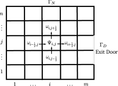
Figure 1. Discretization of the domain $\displaystyle\Omega$.

We define discrete divergence is defined by:

$$(\operatorname{div}_{h}\Phi)_{i,j}=\frac{\Phi^{1}_{i+\frac{1}{2},j}-\Phi^{1}_{i-\frac{1}{2},j}}{h}+\frac{\Phi^{2}_{i,j+\frac{1}{2}}-\Phi^{2}_{i,j-\frac{1}{2}}}{h}.$$ (3.46)

To take into account the Neumann boundary condition $\displaystyle\Phi\cdot\bm{\nu}=0$ on $\displaystyle\Gamma_{N}$, we impose:

• $\displaystyle\Phi_{\frac{1}{2},j}^{1}=0$, for $\displaystyle 1\leq j\leq n$,

• $\displaystyle\Phi_{m+\frac{1}{2},j}^{1}=0,\leavevmode\nobreak\ \text{if}\>((m+\frac{1}{2})h,jh)\in\Gamma_{N}$ ,

• $\displaystyle\Phi_{i,\frac{1}{2}}^{2}=0$, for $\displaystyle 1\leq i\leq m$,

• $\displaystyle\Phi_{i,n+\frac{1}{2}}^{2}=0$, for $\displaystyle 1\leq i\leq m.$

We can rewrite this in a more compact way

$$(\operatorname{div}_{h}\Phi)_{i,j}^{1} =D^{1}_{p}\Phi^{1}_{i,j},\leavevmode\nobreak\ \text{if}\>((m+\frac{1}{2})h,jh)\in\Gamma_{D},$$ (3.47)

$$(\operatorname{div}_{h}\Phi)_{i,j}^{1} =D^{1}_{m}\Phi^{1}_{i,j},\leavevmode\nobreak\ \text{if}\>((m+\frac{1}{2})h,jh)\in\Gamma_{N},$$

$$(\operatorname{div}_{h}\Phi)_{i,j}^{2} =D^{2}\Phi^{2}_{i,j},$$

where the matrices $\displaystyle D^{1}_{m},D^{1}_{p},D^{2}$ are recalled in Appendix-A. Then, we define the discrete gradient operator as follows:

$$(\nabla_{h}p)^{1}_{i,j} =\leavevmode\nobreak\ -^{t}D^{1}_{p}p(i,j),\leavevmode\nobreak\ \text{if}\>((m+\frac{1}{2})h,jh)\in\Gamma_{D},$$ (3.48)

$$(\nabla_{h}p)^{1}_{i,j} =\leavevmode\nobreak\ -^{t}D^{1}_{m}p(i,j),\leavevmode\nobreak\ \text{if}\>((m+\frac{1}{2})h,jh)\in\Gamma_{N},$$

$$(\nabla_{h}p)^{2}_{i,j} =\leavevmode\nobreak\ -^{t}D^{2}p(i,j).$$

This being said, one can easily check that $\displaystyle\operatorname{div}_{h}=-\nabla_{h}^{*}$.

Discretization of the transport equation (2.12) : We use a splitting method as follows. Given a final time $\displaystyle T>0$ and a timestep $\displaystyle\tau>0$, we decompose the interval $\displaystyle[0,T]$ into subintervals $\displaystyle[t_{k},t_{k+\frac{1}{2}}]$ and $\displaystyle[t_{k+\frac{1}{2}},t_{k+1}]$, with $\displaystyle k=0,\dotsc,n-1$. On each interval $\displaystyle[t_{k},t_{k+\frac{1}{2}}]$ we solve the following continuity equation

$$\left\{\begin{aligned} \partial_{t}\rho+\operatorname{div}(V\rho)&=0\\ \rho(t_{k})&=\rho^{k-1},\end{aligned}\right.$$ (3.49)

to obtain $\displaystyle\rho^{k+\frac{1}{2}}$, where $\displaystyle V=(V^{x},V^{y})$ is the velocity field given by $\displaystyle V=-\nabla\mathbf{D}/\|\nabla\mathbf{D}\|$, and $\displaystyle\mathbf{D}$ being the distance (not necessary euclidean) to the boundary $\displaystyle\Gamma_{D}$ given by the eikonal equation (2.13) whose resolution is recalled in Appendix-B. Solving (3.49) can be done by combining a finite difference method in the time variable combined with a $\displaystyle 2$D finite volume method in the space variable. We approximate the term $\displaystyle\operatorname{div}(V\rho)$ in the cell $\displaystyle C_{i,j}=[x_{i-\frac{1}{2},j},x_{i+\frac{1}{2},j}]\times[y_{i,j-\frac{1}{2}},y_{i,j+\frac{1}{2}}]$ as follow:

$$(\operatorname{div}(V\rho))_{i,j}=\frac{1}{\Delta x}[\rho_{i+\frac{1}{2},j}V^{x}_{i+\frac{1}{2},j}-\rho_{i-\frac{1}{2},j}V^{x}_{i,j}]+\frac{1}{\Delta y}[\rho_{i,j+\frac{1}{2}}V^{y}_{i,j+\frac{1}{2}}-\rho_{i,j-\frac{1}{2}}V^{x}_{i,j-\frac{1}{2}}],$$

where $\displaystyle(\operatorname{div}(V\rho))_{i,j}$ the value of $\displaystyle\operatorname{div}(V\rho)$ in the cell $\displaystyle C_{i,j}$ and $\displaystyle(\Delta x,\Delta y)$ are the spatial discretization. Notice that in practice, we take $\displaystyle\Delta x=\Delta y=h$, where $\displaystyle h$ is the mesh size introduced above.

For the time disctization, we use the Euler explicit method to approximate the time derivative of the density. The overall scheme can the be written as:

$$\frac{\rho_{i,j}^{k+\frac{1}{2}}-\rho_{i,j}^{k}}{\tau}+\frac{1}{\Delta x}[\rho_{i+\frac{1}{2},j}^{k}V^{x}_{i+\frac{1}{2},j}-\rho_{i-\frac{1}{2},j}^{k}V^{x}_{i-\frac{1}{2},j}]+\frac{1}{\Delta y}[\rho_{i,j+\frac{1}{2}}^{k}V^{y}_{i,j+\frac{1}{2}}-\rho_{i,j-\frac{1}{2}}^{k}V^{x}_{i,j-\frac{1}{2}}]=0$$ (3.50)

where $\displaystyle\rho_{i,j}^{k+\frac{1}{2}}$ is the average value of $\displaystyle\rho$ in the cell $\displaystyle C_{i,j}=[x_{i-\frac{1}{2},j},x_{i+\frac{1}{2},j}]\times[y_{i,j-\frac{1}{2}},y_{i,j+\frac{1}{2}}]$ at time $\displaystyle({k+\frac{1}{2}})\tau$, and $\displaystyle\rho_{i+\frac{1}{2},j}^{k}$, $\displaystyle V^{x}_{i+\frac{1}{2},j}$ are the values of $\displaystyle\rho$ and $\displaystyle V$at the interface $\displaystyle x_{i+\frac{1}{2},j}$ at time $\displaystyle k\tau$ respectively. Similarly, $\displaystyle(\rho_{i-\frac{1}{2},j}^{k}V^{x}_{i-\frac{1}{2},j})$, $\displaystyle(\rho_{i,j+\frac{1}{2}}^{k},V^{y}_{i,j+\frac{1}{2}})$ and $\displaystyle(\rho_{i,j-\frac{1}{2}}^{k},V^{x}_{i,j-\frac{1}{2}})$ are the values, at time $\displaystyle\tau k$, of $\displaystyle(\rho,V)$ at the interface $\displaystyle x_{i-\frac{1}{2},j}$, $\displaystyle y_{i,j+\frac{1}{2}}$ and $\displaystyle y_{i,j-\frac{1}{2}}$ respectively.

Using the upwind scheme we have $\displaystyle\rho_{i+\frac{1}{2},j}^{k}=\rho_{i,j}^{k}$ and $\displaystyle\rho_{i,j+\frac{1}{2}}^{k}=\rho_{i,j}^{k}$. Substituting in (3.50), the density $\displaystyle\rho_{i,j}^{k+\frac{1}{2}}$ can be written as:

$$\rho_{i,j}^{k+\frac{1}{2}}=\rho_{i,j}^{k}-\frac{\tau}{\Delta x}[\rho_{i,j}^{k}V^{x}_{i+\frac{1}{2},j}-\rho_{i-1,j}^{k}V^{x}_{i-\frac{1}{2},j}]-\frac{\tau}{\Delta y}[\rho_{i,j}^{k}V^{y}_{i,j+\frac{1}{2}}-\rho_{i,j-1}^{k}V^{x}_{i,j-\frac{1}{2}}]$$ (3.51)

We consider that no flux is entering the room from the walls at $\displaystyle\Gamma_{N}$. This is equivalent to impose $\displaystyle\rho_{i-\frac{1}{2},j}^{k}V^{x}_{i-\frac{1}{2},j}=0$ and $\displaystyle\rho_{i,j-\frac{1}{2}}^{k}V^{y}_{i,j-\frac{1}{2}}=0$ at $\displaystyle i=1$ and $\displaystyle j=1$ respectively.
Finally, let us recall that the values of $\displaystyle h$ and $\displaystyle\tau$ are chosen to satisfy a CFL-type constraint $\displaystyle\max(\|V_{i,j}\|)\frac{\tau}{h}<\frac{1}{2}$ in order to guarantee the stability of the numerical scheme (3.50). We summarize this in the following algorithm:

Algorithm 1 Prediction step

1st step. Initialization: Compute the velocity $\displaystyle V=(V^{x},V^{y})$. Choose $\displaystyle\Delta x=\Delta y=h$ and $\displaystyle\tau$ such $\displaystyle\max(\|V_{i,j}\|)\frac{\tau}{h}<\frac{1}{2}$ and take a initial density given by $\displaystyle\rho_{i,j}^{k}$ at time $\displaystyle k\tau$.

2nd step. Update the density at time $\displaystyle(k+\frac{1}{2})\tau$ by

$$\rho_{i,j}^{k+\frac{1}{2}}=\rho_{i,j}^{k}-\frac{\tau}{\Delta x}[\rho_{i,j}^{k}V^{x}_{i+\frac{1}{2},j}-\rho_{i-1,j}^{k}V^{x}_{i-\frac{1}{2},j}]-\frac{\tau}{\Delta y}[\rho_{i,j}^{k}V^{y}_{i,j+\frac{1}{2}}-\rho_{i,j-1}^{k}V^{x}_{i,j-\frac{1}{2}}].$$

Remark 3.10.

The discretization of $\displaystyle\operatorname{div}(V\>\rho)$ assumes a positive direction for the speed i.e., $\displaystyle V^{x}>0$ and $\displaystyle V^{y}>0$. However, the scheme can be easily adapted to other cases. For example, if $\displaystyle V^{x}>0$ and $\displaystyle V^{y}<0$ for some $\displaystyle(i,j)$, the discretization of $\displaystyle\operatorname{div}(\rho V)$ becomes:

$$(\operatorname{div}(V\rho))_{i,j}=\frac{1}{\Delta x}[\rho_{i+\frac{1}{2},j}V^{x}_{i+\frac{1}{2},j}-\rho_{i-\frac{1}{2},j}V^{x}_{i-\frac{1}{2},j}]+\frac{1}{\Delta y}[\rho_{i,j-\frac{1}{2}}V^{y}_{i,j-\frac{1}{2}}-\rho_{i,j+\frac{1}{2}}V^{x}_{i,j+\frac{1}{2}}],$$ (3.52)

Since the obtained density $\displaystyle\rho^{k+\frac{1}{2}}$ may violate the constraint $\displaystyle\rho\leq 1$, the next step is to handle congestion by solving the following minimum flow problem

$$\inf_{(\rho,\Phi)}\left\{\int_{\Omega}\mathsf{k}(x)|\Phi(x)|\mathrm{d}x:\leavevmode\nobreak\ -\tau\>\operatorname{div}(\Phi)=\rho^{k+\frac{1}{2}}-\rho\hbox{ in }\Omega,\ \Phi\cdot\nu=0\hbox{ on }\Gamma_{N}\mbox{ and }0<\rho\leq 1\right\},$$ (3.53)

where where $\displaystyle\mathsf{k}\geq 0$ is a continuous function and, for the simplicity of the presentation, we take vanishing $\displaystyle g$ and $\displaystyle\eta$ (see Remark 3.11).

Discretization of the minimum flow problem (3.53) : First, let us rewrite (3.53) in the form

$$\textup{(M)}:\leavevmode\nobreak\ \leavevmode\nobreak\ \min_{(\rho,\Phi)}\mathcal{A}(\rho,\Phi)+\mathbb{I}_{\mathcal{C}}(\Lambda(\rho,\Phi)),$$ (3.54)

where (we omit the variable $\displaystyle\tau$ to lighten the notation)

$$\mathcal{A}(\rho,\Phi)=\int_{\Omega}\tau\mathsf{k}(x)|\Phi(x)|\mathrm{d}x+\mathbb{I}_{[0,1]}(\rho),\quad\Lambda(\rho,\Phi)=\rho-\tau\operatorname{div}\Phi\quad\mbox{and}\leavevmode\nobreak\ \mathcal{B}=\mathbb{I}_{\left\{\rho^{k+\frac{1}{2}}\right\}}.$$

This problem can be efficiently solved by Chambolle-Pock’s primal-dual algorithm (PD) (c.f. [7]).

Based on the discrete gradient and divergence operators, we propose a discrete version of (M) as follows

$$\textup{(M)}_{d}:\leavevmode\nobreak\ \min\limits_{\begin{subarray}{c}(\rho,\Phi)\end{subarray}}\Big{\{}h^{2}\sum_{i=1}^{m+1}\sum_{j=1}^{n+1}\tau\mathsf{k}_{i,j}\|\Phi_{i,j}\|+\mathbb{I}_{[0,1]}(\rho)+\mathbb{I}_{\mathcal{C}}(\Lambda_{h}(\rho,\Phi))\Big{\}}$$ (3.55)

where $\displaystyle\mathcal{C}:=\left\{(a_{i,j})\>:\>a_{i,j}=\rho_{i,j}^{k+\frac{1}{2}},\leavevmode\nobreak\ \leavevmode\nobreak\ \forall(i,j)\in\llbracket 1,m\rrbracket\times\llbracket 1,n\rrbracket\right\},$ $\displaystyle\Lambda_{h}(\rho,\Phi)=\rho-\tau\operatorname{div}_{h}\Phi$ and $\displaystyle\mathsf{k}_{i,j}$ is the value of $\displaystyle\mathsf{k}$ in $\displaystyle C_{i,j}$. In other words, the discrete version $\displaystyle\textup{(M)}_{d}$ can be written as

$$\min_{(\rho,\Phi)}\mathcal{A}_{h}(\rho,\Phi)+\mathcal{B}_{h}(\Lambda_{h}(\rho,\Phi)),$$ (3.56)

or in a primal-dual form as

$$\min_{(\rho,\Phi)}\max_{p}\mathcal{A}_{h}(\rho,\Phi)+\langle u,\Lambda_{h}(\rho,\Phi)\rangle-\mathcal{B}_{h}^{*}(p),$$ (3.57)

where

$$\mathcal{A}_{h}(\rho,\Phi)=h^{2}\sum_{i=1}^{m+1}\sum_{j=1}^{n+1}\tau\mathsf{k}_{i,j}\|\Phi_{i,j}\|+\mathbb{I}_{[0,1]}(\rho)\leavevmode\nobreak\ \mbox{and}\leavevmode\nobreak\ \mathcal{B}_{h}=\mathbb{I}_{\mathcal{C}}.$$ (3.58)

Notice that in this case, (2.69) has a dual problem that reads

$$\min\limits_{\begin{subarray}{c}\rho\in X\\ 0\leq\rho\leq 1\end{subarray}}\max\limits_{\begin{subarray}{c}p\in X\\ p=0\text{ on }\Gamma_{D}\end{subarray}}h^{2}\left\{\sum_{i=1}^{m}\sum_{j=1}^{n}p_{i,j}(\rho_{i,j}^{k+\frac{1}{2}}-\rho_{i,j}):\leavevmode\nobreak\ \|\nabla_{h}p_{i,j}\|\leq\mathsf{k}_{i,j}\right\}.$$ (3.59)

Then (PD) algorithm [8] can be applied to $\displaystyle\textup{(M)}_{d}$ as follows:

Algorithm 2 (PD) iterations

1st step. Initialization: choose $\displaystyle\alpha,\beta>0$, $\displaystyle\theta\in[0,1]$, $\displaystyle\rho_{0},\Phi^{0}$ and take $\displaystyle u_{0}=\Lambda_{h}(\rho^{0},\Phi^{0}),\>\bar{p}^{0}=p^{0}$

2nd step. For $\displaystyle l\leq\mathrm{Iter}_{max}$ do

$$(\rho^{l+1},\Phi^{l+1}) =\textbf{Prox}_{\beta\mathcal{A}_{h}}\left((\rho^{l},\Phi^{l})-\beta\Lambda_{h}^{*}(\bar{p}^{l})\right);$$

$$p^{l+1} =\textbf{Prox}_{\alpha\mathcal{B}_{h}^{*}}\left(p^{l}+\alpha\Lambda_{h}(\rho^{l+1},\Phi^{l+1})\right);$$

$$\bar{p}^{l+1} =p^{l+1}+\theta(p^{l+1}-p^{l}).$$

Recall here that the proximal operator is defined through

$$\textbf{Prox}_{\alpha E}(p)=\underset{q}{\operatorname{argmin}}\frac{1}{2}\|p-q\|^{2}+\eta E(q).$$ (3.60)

3.2. Computation of the proximal operators

See that for the functional $\displaystyle\mathcal{A}_{h}$ and $\displaystyle\mathcal{B}_{h}^{*}$ can be computed explicitly. Indeed, the functional $\displaystyle\mathcal{A}_{h}$ is separable in the variables $\displaystyle\rho$ and $\displaystyle\Phi$ :

$$\mathcal{A}_{h}(\rho,\Phi)=\mathbb{I}_{[0,1]}(\rho)+\|\Phi\|_{1}.$$

So, $\displaystyle\textbf{Prox}_{\eta\mathcal{A}_{h}}$ is the some of a projection in the first component and the so-called soft-thresholding. Namely

$$\left(\textbf{Prox}_{\mathcal{A}_{h}}(\rho,\Phi)\right)_{i,j}=\left(\max(0,\min(1,\rho_{i,j})),\max(0,1-\frac{1}{|\Phi_{i,j}|})\Phi_{i,j}\right).$$ (3.61)

As to $\displaystyle\mathcal{B}_{h}^{*},$ in order to compute $\displaystyle\textbf{Prox}_{\alpha\mathcal{B}^{*}_{h}}$, we make use of Moreau’s identity

$$p=\textbf{Prox}_{\alpha\mathcal{B}^{*}_{h}}(p)+\alpha\textbf{Prox}_{\alpha^{-1}\mathcal{B}_{h}}(p/\eta),$$ (3.62)

and the fact that $\displaystyle\textbf{Prox}_{\alpha^{-1}\mathcal{B}_{h}}(a,b)$ is given simply by the projection onto $\displaystyle\mathcal{C}$. Consequently,

$$\left(\textbf{Prox}_{\alpha\mathcal{B}^{*}_{h}}(p)\right)_{i,j}=\left(p_{i,j}-\alpha\textbf{Proj}_{\mathcal{C}_{i,j}}(p_{i,j}/\alpha)\right).$$

Thus, the details of Algorithm 3 to solve $\displaystyle\textup{(M)}_{d}$ are as follow :

Algorithm 3 (PD) iterations for $\displaystyle\textup{(M)}_{d}$

Initialization: Let $\displaystyle k=0$, choose $\displaystyle\alpha,\beta>0$ such that $\displaystyle\alpha\beta\|\Lambda_{h}\|^{2}<1$. Choose $\displaystyle\rho^{0},\Phi^{0}$ and $\displaystyle p^{0}=\bar{p}^{0}=p_{0}$.

Primal step:

$$(\rho_{i,j}^{l+1},\Phi_{i,j}^{l+1})=\left(\max\Big{(}0,\min(1,\rho_{i,j}^{l}-\beta\bar{p}^{l}_{i,j})\Big{)},\max\Big{(}0,1-\frac{1}{|\Phi_{i,j}^{l}-\beta\nabla_{h}\bar{p}_{i,j}^{l}|}\Big{)}\Big{(}\Phi_{i,j}^{l}-\beta\nabla_{h}\bar{p}_{i,j}^{l}\Big{)}\right).$$ (3.63)

Dual step:

$$v^{l+1} =p^{l}+\alpha\rho^{l+1}-\alpha\operatorname{div}_{h}(\Phi^{l+1}).$$ (3.64)

$$p^{l+1}_{i,j} =v^{l+1}_{i,j}-\alpha\textbf{Proj}_{\mathcal{C}_{i,j}}(v_{i,j}^{l+1}/\alpha),\>1\leq i\leq m,1\leq j\leq n.$$

Extragradient:

$$\bar{p}^{l+1}=2p^{l+1}-p^{l}.$$

It was shown in [8] that when $\displaystyle\theta=1$ and $\displaystyle\alpha\beta\|\Lambda_{h}\|^{2}<1$, the sequence $\displaystyle\{(\rho^{l},\Phi^{l})\}$ converges to an optimal solution of $\displaystyle\textup{(M)}_{d}$. So in practice, we choose $\displaystyle\alpha>0$ and we take $\displaystyle\beta=1/(\eta K^{2})$, where $\displaystyle K$ is an upper bound of $\displaystyle\|\Lambda_{h}\|$. More precisely, $\displaystyle K=\sqrt{\|\nabla_{h}\|^{2}+\|\mathrm{id}_{X}\|^{2}}\equiv\|\Lambda_{h}\|$. The algorithm was implemented in Matlab and all the numerical examples below were executed on a 2,6 GHz CPU running macOs High Sierra system.

Remark 3.11 (Non-homogeneous Neuman boundary condition : non null $\displaystyle\eta$).

In is not difficult to see that in the case of non null $\displaystyle\eta,$ one can handle this case by considering $\displaystyle\eta$ as a source term on the boundary on $\displaystyle\Gamma_{N}.$ To avoid numerical computation for the correction we propose to handle the condition

$$-\tau\>\operatorname{div}(\Phi)=\rho_{k+1/2}-\rho\hbox{ in }\mathcal{D}^{\prime}(\Omega)\hbox{ and }\Phi\cdot\bm{\nu}=\eta\hbox{ on }\Gamma_{N}.$$

as

$$-\tau\>\operatorname{div}(\Phi)=\rho_{k+1/2}+\tau\>\eta-\rho\hbox{ in }\mathcal{D}^{\prime}(\overline{\Omega}\setminus\Gamma_{D}).$$

In other words, at each iteration we take $\displaystyle\rho^{l}+\tau\>\eta$ instead of $\displaystyle\rho^{l}$ in the Algorithms 1-2.

4. Numerical simulations

In this section we present several examples to illustrate our approach . We first examine the scenario of evacuation of a population $\displaystyle\rho_{0}$ from a the domain $\displaystyle\Omega\subset\mathbb{R}^{2}$ via an exit $\displaystyle\Gamma_{D}$ with different velocities. In the last two examples we compare our approach to the one in [31, 32], the configuration in the first one is similar to the previous ones, i.e., the crowed is initially located in a part of the room $\displaystyle\Omega$ and try to escape through the doors, while in the second example the domain $\displaystyle\Omega$ is constituted by two rooms connected by a ”bridge”. In all these examples, the velocity field $\displaystyle V$ derives from a potential $\displaystyle\varphi$ that is considered as the distance function to the door $\displaystyle\Gamma_{D}$ and is computed by solving the eikonal equation

$$\left\{\begin{aligned} \|\nabla\varphi\|&=f(\textbf{x})\\ \varphi_{\mid\Gamma_{D}}&=0,\end{aligned}\right.$$ (4.65)

using the primal-dual method proposed in [19] (see also [21]), where $\displaystyle f\geq 0$ is a continuous function that will be precised for each example. All the tests of this section are performed with a mesh size $\displaystyle h=0.01$ and a timestep $\displaystyle\tau=0.004$. Moreover, the corresponding velocities are displayed in red.

4.1. One room evacuation

In this first example (c.f. Figure-2), the initial density $\displaystyle\rho_{0}$ is given by $\displaystyle\rho_{0}(\textbf{x})=\mathbf{1}_{S_{1}}(\textbf{x})+\mathbf{1}_{S_{2}}(\textbf{x})$ with $\displaystyle S_{1}=[0,\frac{1}{2}]\times[0,\frac{1}{3}]$ and $\displaystyle S_{2}=[0,\frac{1}{2}]\times[\frac{2}{3},1]$. The exit is given by $\displaystyle\Gamma_{D}=\{1\}\times[0.4,0.6]$ and $\displaystyle f\equiv 1$.

Figure 2. The crowed density $\displaystyle\rho$ computed at 6 different timesteps with $\displaystyle T=2$ and $\displaystyle f\equiv 1$.

In the second example (c.f. Figure-3), the initial density is $\displaystyle\rho_{0}(\textbf{x})=\mathbf{1}_{S_{1}}(\textbf{x})$ with $\displaystyle S_{1}=[0,\frac{1}{2}]\times[0,1]$ and $\displaystyle\Gamma_{D}=\left(\{1\}\times[0,0.4]\right)\cup\left(\{1\}\times[0.9,1]\right)$ and $\displaystyle f(\textbf{x})=e^{-3\times\left((x-\frac{1}{2})^{2}+(y-\frac{1}{2})^{2}\right)}$.

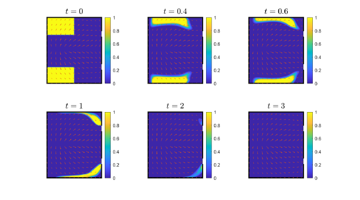
Figure 3. The crowed density $\displaystyle\rho$ computed at 6 different timesteps with $\displaystyle T=3$ and $\displaystyle f(\textbf{x})=e^{-3\times\left((x-\frac{1}{2})^{2}+(y-\frac{1}{2})^{2}\right)}$.

In this example, the function $\displaystyle f$ has a bump in the middle of the domain, and we can observe in Figure-3 that the population is avoiding this region while heading the doors.

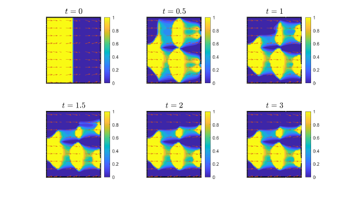
Figure 4. The crowed density $\displaystyle\rho$ computed at 6 different timesteps with $\displaystyle T=3$ and $\displaystyle f(\textbf{x})=|\cos(3x+5y)|+0.2$.

In the third example (c.f. Figure-4),, the initial condition for the density is $\displaystyle\rho_{0}(\textbf{x})=\mathbf{1}_{S_{1}}(\textbf{x})$ with $\displaystyle S_{1}=[0,\frac{1}{2}]\times[0,1]$ and $\displaystyle\Gamma_{D}=\left(\{1\}\times[0.2,0.3]\right)\cup\left(\{1\}\times[0.7,0.8]\right)$ and $\displaystyle f(\textbf{x})=|\cos(3x+5y)|+0.2$. The source term is located on the entry of the domain at $\displaystyle\Gamma_{S}=\{0\}\times[0.3,0.6]$.
In this example one sees that the vector filed of spontaneous velocity has small values in successive (periodic) regions. This produce in turns successive congestion zones. Moreover, the system reaches its equilibrium after $\displaystyle t=2$. One can notice that no variation in the density is observed as the number of persons leaving the room is equal to the number of person entering the room.

4.2. Homogeneous case vs quadratic case

As we pointed out in Subsection-2.3, in the case where $\displaystyle F(x,\xi)=|\xi|$, our model is connected to the gradient flow in the Wasserstein space equipped with $\displaystyle\mathds{W}_{1}$. Whereas the case $\displaystyle F(x,\xi)=\frac{1}{2}|\xi|^{2}$ can be related to the gradient flow in the Wasserstein space equipped with the $\displaystyle\mathds{W}_{2}$ distance (c.f. [31, 32]), where decongestion is performed using the Laplace operator as we discussed in Remark-2.8. The solution of the continuity equation is computed first (prediction step), then it is projected onto the set of admissible densities with respect to $\displaystyle\mathds{W}_{2}$-Wasserstein distance (correction step). Using our approach, this can be simply solved by changing the functional $\displaystyle\mathcal{A}_{h}$ to $\displaystyle\mathcal{A}_{h}(\rho,\Phi)=\mathbb{I}_{[0,1]}(\rho)+1/2\|\Phi\|_{2}^{2}$ and modifying formula (3.61) using the fact that

$$\textbf{Prox}_{\frac{\sigma}{2}\|.\|_{2}^{2}}(\Phi)=\frac{1}{1+\sigma}\Phi.$$ (4.66)

To observe differences between the two methods, we consider two examples. In the first one (c.f. Figure-5), the initial density is $\displaystyle\rho_{0}(\textbf{x})=\mathbf{1}_{S_{1}}(\textbf{x})$ with

$$S_{1}=[0,\frac{1}{2}]\times[0,1]\leavevmode\nobreak\ \mbox{and}\leavevmode\nobreak\ \Gamma_{D}=\left(\{1\}\times[0,0.4]\right)\cup\left(\{1\}\times[0.9,1]\right).$$

.

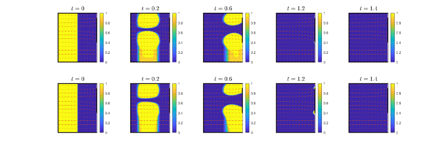
Figure 5. The distribution of crowd at equivalent timesteps with $\displaystyle T=2$. Top row: result using our approach. Bottom row: result using the Laplacian.

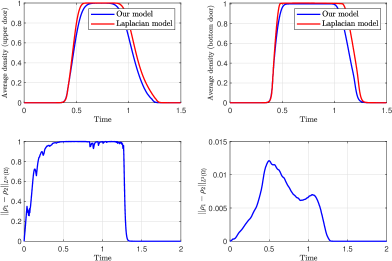
Figure 6. Top: Variation of the average density over time for the two models at the exist doors. Bottom: Variation of $\displaystyle||\rho_{1}-\rho_{2}||_{L^{\infty}(\Omega)}$ and $\displaystyle||\rho_{1}-\rho_{2}||_{L^{2}(\Omega)}$ as a function of time for the two rooms case. $\displaystyle\rho_{1}$ is the solution obtained by our approach and $\displaystyle\rho_{2}$ the solution obtained by the Laplacian model.

Now, we consider a domain $\displaystyle\Omega=[0,1]^{2}=\Omega_{l}\cup\Omega_{r}$ composed of two rooms linked by a bridge in the spirit of [30], where $\displaystyle\Omega_{l}=[0,0.4]\times[0,1]$ and $\displaystyle\Omega_{r}=[0.6,1]\times[0,1]$. The initial density $\displaystyle\rho_{0}$ is located at the left room and is given by $\displaystyle\rho_{0}(\textbf{x})=\mathbf{1}_{S}(\textbf{x})$ with $\displaystyle S=[0,0.4]\times[0,1]$ . The exit is given by the two end points $\displaystyle(1,0)$ and $\displaystyle(1,1)$, that is $\displaystyle\Gamma_{D}=\{(1,0),(1,1)\}$.

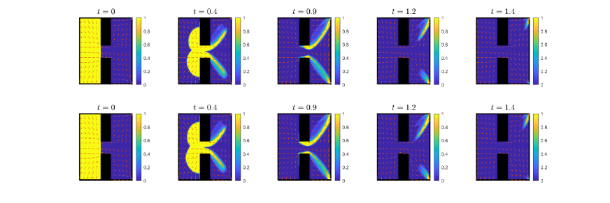
Figure 7. The distribution of the crowd over the domain at equivalent timesteps. Top row: result using our approach. Bottom row: result using the Laplacian.

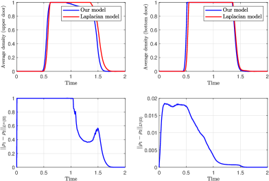
Figure 8. Top: Variation of the average density over time for the two models at the exist doors. Bottom: Variation of $\displaystyle||\rho_{1}-\rho_{2}||_{L^{\infty}(\Omega)}$ and $\displaystyle||\rho_{1}-\rho_{2}||_{L^{2}(\Omega)}$ as a function of time for the two rooms case. $\displaystyle\rho_{1}$ is the solution obtained by our approach and $\displaystyle\rho_{2}$ the solution obtained by the Laplacian model.

Figures-5-7 provide a comparison between our method to and one using the Laplace operator in equivalent timesteps. Overall, both models behave similarly except that our model seems to perform faster evacuation. In most of the timesteps examples, it is difficult to visualize differences in of the evolution of the crowd only through the figures. Yet, we can observe this by measuring the $\displaystyle L^{\infty}$ and $\displaystyle L^{2}$ norms of the obtained solutions as well as the variation of the average density over time for the two models at the exist doors. Thanks to Figures-6-8, one can clearly notice that our model is faster than the Laplacian model in achieving population evacuation, as the blue curve (our model) remains under the red curve (Laplacian model) over all the time period.

4.3. Evacuation with path obstacles

In this section, we analyse the evacuation process in the presence of in-domain obstacles. At the microscopic level, it was shown in [37] that pedestrians might be blocked from exiting the room in case where no obstacle is placed in front of the exist. The reason is that pedestrians start to push each other once near to the exist blocking the continuation of the evacuation process. The authors [37] have concluded that placing an obstacle just in front of the exist regulates the evacuation and avoids blocking of pedestrians. To observe the effect of placing an obstacle in front in the exist on the fluidity and speed of the evacuation in the macroscopic case, we consider the following example in $\displaystyle\Omega=[0,1]^{2}$ where the obstacle is placed at the region $\displaystyle[0.8,0.9]\times[0.2,0.7]$. The initial density $\displaystyle\rho_{0}$ is located at the left room and is given by $\displaystyle\rho_{0}(\textbf{x})=\mathbf{1}_{S}(\textbf{x})$ with $\displaystyle S=[0,0.5]\times[0,1]$ . The exit is given by $\displaystyle\Gamma_{D}={1}\times[0.4,0.6]$.

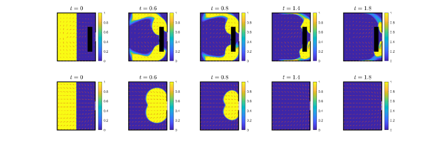
Figure 9. The distribution of the crowd over the domain at equivalent timesteps.

As shown in Figure-9, we can notice that after $\displaystyle t=1.4$, the room is completely evacuated in absence of the obstacle in front of the exist. However, when considering obstacle we can notice that the evacuation is partial and some pedestrian are stuck in the room. In fact, placing an obstacle slowed down the evacuation.
Unlike the microscopic case, adding an obstacle in the macroscopic case have had negative effects on the evacuation process due to the continum model of the density.

Appendix A On the discrete operators

In this section, we recall some details concerning the discrete divergence and gradient operators that were used in Section-3. First, let us recall that the space $\displaystyle X=\mathbb{R}^{m\times n}$ is equipped with a scalar product and an associated norm as follows:

$$\langle u,v\rangle=h^{2}\sum_{i=1}^{m}\sum_{j=1}^{n}u_{i,j}v_{i,j}\quad\mbox{ and }\quad\|u\|=\sqrt{\langle u,u\rangle},$$

where $\displaystyle h$ is a given mesh size. Following the definition of the discrete divergence operator given in (3.46), the discrete gradient $\displaystyle\nabla_{h}:X\longrightarrow Y=\mathbb{R}^{(m+1)\times n}\times\mathbb{R}^{m\times(n+1)}$ is given by $\displaystyle(\nabla_{h}u)_{i,j}=\Big{(}(\nabla_{h}u)^{1}_{i,j},(\nabla_{h}u)^{2}_{i,j}\Big{)}$, where

$$(\nabla_{h}u)^{1}_{i,j} =\leavevmode\nobreak\ -^{t}D^{1}_{p}u(i,j),\leavevmode\nobreak\ \text{if}\>((m+\frac{1}{2})h,jh)\in\Gamma_{D},$$ (1.67)

$$(\nabla_{h}u)^{1}_{i,j} =\leavevmode\nobreak\ -^{t}D^{1}_{m}u(i,j),\leavevmode\nobreak\ \text{if}\>((m+\frac{1}{2})h,jh)\in\Gamma_{N},$$

$$(\nabla_{h}u)^{2}_{i,j} =\leavevmode\nobreak\ -^{t}D^{2}u(i,j).$$

and the matrices $\displaystyle D^{1}_{P},D^{2}_{m}$, $\displaystyle D^{2}$ are given by

$$D^{1}_{p}=\scriptsize{\begin{pmatrix}0&1/h&0&\cdots&&&0\\ 0&-1/h&1/h&0&\cdots&&0\\ 0&0&-1/h&1/h&0&\cdots&0\\ \vdots&&\vdots&\ddots&&\vdots\\ 0&0&\cdots&&0&-1/h&1/h\end{pmatrix}}$$

$$D^{1}_{m}=\scriptsize{\begin{pmatrix}0&1/h&0&\cdots&&&0\\ 0&-1/h&1/h&0&\cdots&&0\\ 0&0&-1/h&1/h&0&\cdots&0\\ \vdots&&\vdots&\ddots&&\vdots\\ 0&0&\cdots&&0&-1/h&0\end{pmatrix}}$$

and

$$D^{2}=\scriptsize{\begin{pmatrix}0&1/h&0&\cdots&&&0\\ 0&-1/h&1/h&0&\cdots&&0\\ 0&0&-1/h&1/h&0&\cdots&0\\ \vdots&&\vdots&\ddots&&\vdots\\ 0&0&\cdots&&0&-1/h&0\end{pmatrix}}.$$

This being said, we check easily that $\displaystyle-\operatorname{div}_{h}$ and $\displaystyle\nabla_{h}$ are in duality. Moreover, we recall the following

Proposition 1.12.

([7, 8]) Under the above-mentioned definitions and notations, one has that

• The adjoint operator of $\displaystyle\nabla_{h}$ is $\displaystyle\nabla^{*}_{h}=-\operatorname{div}_{h}.$

• Its norm satisfies: $\displaystyle\|\nabla_{h}\|^{2}=\|\operatorname{div}_{h}\|^{2}\leq 8/h^{2}$.

Appendix B Discretization of the eikonal equation:

For a self-contained presentation, let us recall our main approach to compute the velocity field $\displaystyle V$ by solving the eikonal equation (2.13). As pointed out in [21] (see also [19]), the solution $\displaystyle\mathbf{D}$ of (2.13) can be obtained by solving

$$\max_{u\in W^{1,\infty}(\Omega)}\left\{\int_{\Omega}u\mathrm{d}\textbf{x}:|\nabla u|\leq f,\leavevmode\nobreak\ u=0\leavevmode\nobreak\ \mbox{on}\leavevmode\nobreak\ \Gamma_{D}\right\}$$ (2.68)

which can be written, at a discrete level, as

$$\min_{u\in X}\mathcal{A}_{h}(u)+\mathcal{B}_{h}(\nabla_{h}u),$$ (2.69)

where

$$\mathcal{A}_{h}(u)=\begin{cases}-h^{2}\sum_{i=1}^{m}\sum_{j=1}^{n}u_{i,j}&\text{ if }u_{i,j}=0\>\>\forall(i,j)\in D_{d}\\ +\infty&\text{ otherwise }\end{cases},\leavevmode\nobreak\ \mbox{and}\leavevmode\nobreak\ \mathcal{B}_{h}=\mathbb{I}_{B(0,f)},$$ (2.70)

where $\displaystyle D_{d}=\left\{(i,j):(ih,jh)\in\Gamma_{D}\right\}$ the indexes whose spatial positions belong to $\displaystyle\Gamma_{D}$ and $\displaystyle B(0,f)$ is the unit ball of radius $\displaystyle f$. Then we apply Algorithm-2 with the functionals $\displaystyle\mathcal{A}_{h}$ and $\displaystyle\mathcal{B}_{h}$ above.

Appendix C Duality results

The idea for the proof of Lemma 2.4 goes back to [19, Theorem 3.10]. The aim is to define a convex and l.s.c functional $\displaystyle\mathcal{H}\>:\>\mathcal{M}_{b}(\overline{\Omega})\mapsto]-\infty,\infty]$ such that

$$\mathcal{H}(0)=\inf_{\tau\Phi\in\mathcal{F}^{q}(\tilde{\rho}-\rho)}\left\{\tau\int_{\Omega}\mathsf{k}(x)\>|\Phi(x)|\>\mathrm{d}x-\tau\int_{\Gamma_{D}}g(x)\>\Phi\cdot\bm{\nu}\>\mathrm{d}x\right\}$$

and

$$\sup_{p\in\mathcal{C}(\overline{\Omega})}-\mathcal{H}^{*}(p)=\max_{p\in\mathcal{G}_{\mathsf{k}}}\left\{\int(\tilde{\rho}-\rho)\>p\>\mathrm{d}x-\tau\>\int_{\Gamma_{N}}p\>\eta\>\mathrm{d}x\right\}.$$

Then conclude by classical duality results

$$\mathcal{H}(0)=\mathcal{H}^{**}(0)=\sup_{p\in\mathcal{C}(\overline{\Omega})}-\mathcal{H}^{*}(p).$$ (3.71)

One sees that in order to built $\displaystyle\mathcal{H}$, we need to use vector fields whose divergences are Radon measures (c.f. [9]). Thanks to [9], we know that for any $\displaystyle\Phi\in L^{1}(\Omega)^{N}$ such that $\displaystyle\operatorname{div}\Phi=:\mu_{\Phi}\in\mathcal{M}_{b}(\Omega),$ in the sense of $\displaystyle\mathcal{D}^{\prime}(\Omega),$ the normal trace of $\displaystyle\Phi$ is well defined on the boundary of $\displaystyle\Omega$. Indeed, for such $\displaystyle\Phi,$ we have $\displaystyle\Phi\cdot\bm{\nu}\>:\>\textup{Lip}(\partial\Omega)\to\mathbb{R}$ is continuous linear functional and satisfies

$$\langle\Phi\cdot\bm{\nu},\xi_{\mid\partial\Omega}\rangle=\int_{\Omega}\xi\>\mathrm{d}\mu_{\Phi}+\int_{\Omega}\Phi\cdot\nabla\xi\>\mathrm{d}x,\quad\hbox{ for any }\xi\in\mathcal{C}^{1}(\overline{\Omega}).$$ (3.72)

We will denote again $\displaystyle\langle\Phi\cdot\bm{\nu},\xi_{\mid\partial\Omega}\rangle=:\int_{\partial\Omega}\Phi\cdot\bm{\nu}\>\xi\>\mathrm{d}x.$ As for $\displaystyle H_{\hbox{div}}$ vector valued field, it is possible to define the restriction of the normal trace of $\displaystyle\Phi$ on $\displaystyle\Gamma_{D}$ by working with Lipschitz continuous test functions which vanishes on $\displaystyle\Gamma_{N}.$ For any $\displaystyle g\in\textup{Lip}(\Gamma_{D})$ such that there exists $\displaystyle\tilde{g}\in\mathcal{C}^{1}(\overline{\Omega}),$ satisfying

$$\tilde{g}=g\hbox{ on }\Gamma_{D}\hbox{ and }\tilde{g}=0\hbox{ on }\Gamma_{N}.$$

For such $\displaystyle g,$ we’ll define $\displaystyle\int_{\Gamma_{D}}\Phi\cdot\bm{\nu}\>g\>\mathrm{d}x:=\langle\Phi\cdot\bm{\nu},\tilde{g}_{\mid\partial\Omega}\rangle$, for any $\displaystyle\Phi\in L^{1}(\Omega)^{N}$; i.e.,

$$\int_{\Gamma_{D}}\Phi\cdot\bm{\nu}\>g\>\mathrm{d}x=\int_{\Omega}\tilde{g}\>\mathrm{d}\mu_{\Phi}+\int_{\Omega}\nabla\tilde{g}\cdot\Phi\>\mathrm{d}x.$$ (3.73)

So, for any $\displaystyle\mu\in\mathcal{M}_{b}(\overline{\Omega}),$ we can define

$$\mathcal{F}(\mu):=\Big{\{}\Phi\in L^{1}(\Omega)^{N}\>:\>-\operatorname{div}(\Phi)=\mu\!\!\mathop{\hbox{ \vrule height=7.0pt,width=0.5pt,depth=0.0pt\vrule height=0.5pt,width=6.0pt,depth=0.0pt}}\nolimits\Omega\hbox{ in }\Omega\hbox{ and }\Phi\cdot\bm{\nu}=\eta+\mu\!\!\mathop{\hbox{ \vrule height=7.0pt,width=0.5pt,depth=0.0pt\vrule height=0.5pt,width=6.0pt,depth=0.0pt}}\nolimits\Gamma_{N}\hbox{ on }\Gamma_{N}\Big{\}}.$$

Here, the condition $\displaystyle-\operatorname{div}(\Phi)=\mu\!\!\mathop{\hbox{ \vrule height=7.0pt,width=0.5pt,depth=0.0pt\vrule height=0.5pt,width=6.0pt,depth=0.0pt}}\nolimits\Omega$ in $\displaystyle\Omega$ and $\displaystyle\Phi\cdot\bm{\nu}=\eta+\mu\!\!\mathop{\hbox{ \vrule height=7.0pt,width=0.5pt,depth=0.0pt\vrule height=0.5pt,width=6.0pt,depth=0.0pt}}\nolimits\Gamma_{N}$ on $\displaystyle\Gamma_{N},$ needs to be understood in the sense

$$\int_{\Omega}\Phi\cdot\nabla\xi\>\mathrm{d}x=\int_{\overline{\Omega}}\xi\>\mathrm{d}\mu+\int_{\Gamma_{N}}\eta\>\xi\>\mathrm{d}x,\quad\hbox{ for any }\xi\in\textup{Lip}(\Omega)\hbox{ s.t. }\xi_{\mid\Gamma_{D}}=0.$$ (3.74)

Proposition 3.13.

For any $\displaystyle\mu\in\mathcal{M}_{b}(\overline{\Omega})$, we have

$$\begin{array}[]{l}\inf_{\tau\Phi\in\mathcal{F}(\mu)}\left\{\tau\int_{\Omega}\mathsf{k}(x)\>|\Phi(x)|\>\mathrm{d}x-\tau\int_{\Gamma_{D}}g(x)\>\Phi\cdot\bm{\nu}\>\mathrm{d}x\right\}\\ \\ \hskip 28.45274pt=\max_{p\in\mathcal{G}_{\mathsf{k}}}\left\{\int_{\overline{\Omega}}p\>\mathrm{d}\mu-\tau\>\int_{\Gamma_{N}}p\>\eta\>\mathrm{d}x\right\}.\end{array}$$ (3.75)

Proof.

We consider on $\displaystyle\mathcal{M}_{b}(\overline{\Omega})$ the following functional $\displaystyle\mathcal{H}\>:\>\mathcal{M}_{b}(\overline{\Omega})\mapsto]-\infty,\infty]$ defined by

$$\mathcal{H}(h)=\inf_{\tau\phi\in\mathcal{F}(\mu+h)}\left\{\tau\int_{{\Omega}}\mathsf{k}(x)\>|\Phi(x)|\mathrm{d}x+\int_{\Gamma_{D}}g\>\mathrm{d}h-\tau\int_{\Gamma_{D}}\Phi\cdot\bm{\nu}\>g\>\mathrm{d}x\right\},$$

for any $\displaystyle h\in\mathcal{M}_{b}(\overline{\Omega}).$ Then $\displaystyle\mathcal{H}$ is convex and l.s.c.

Convexity.

Indeed, take $\displaystyle h_{1},h_{2}\in\mathcal{M}_{b}(\overline{\Omega})$ and set $\displaystyle h:=th_{1}+(1-t)h_{2}$ for $\displaystyle t\in[0,1]$. Let $\displaystyle\Phi_{1,n},\Phi_{2,n}\in L^{1}(\Omega)^{N}$ be two minimizing sequences of fluxes corresponding to $\displaystyle h_{1}$ and $\displaystyle h_{2}$ respectively, i.e., $\displaystyle\tau\Phi_{1,n}\in\mathcal{F}(\mu+h_{1})$ and $\displaystyle\tau\Phi_{2,n}\in\mathcal{F}(\mu+h_{2})$ such that

$$\mathcal{H}(h_{i})=\tau\lim_{n}\int_{{\Omega}}\mathsf{k}(x)|\Phi_{i,n}(x)|\mathrm{d}x+\int_{\Gamma_{D}}g\>\mathrm{d}h_{i}-\tau\int_{\Gamma_{D}}\Phi_{i,n}\cdot\bm{\nu}\>g\>\mathrm{d}x\leavevmode\nobreak\ \leavevmode\nobreak\ \text{ for}\leavevmode\nobreak\ \leavevmode\nobreak\ i=1,2.$$

Set $\displaystyle\Phi_{n}=t\Phi_{1,n}+(1-t)\Phi_{2,n}$. We clearly see that $\displaystyle\phi_{n}$ are admissible for $\displaystyle h$ and

$$\displaystyle\mathcal{H}(h) \displaystyle\leq\tau\lim_{n}\int_{{\Omega}}\mathsf{k}(x)|\Phi_{n}(x)|\mathrm{d}x+\int_{\Gamma_{D}}g\>\mathrm{d}h-\tau\int_{\Gamma_{D}}\Phi_{n}\cdot\bm{\nu}\>g\>dx$$

$$\displaystyle=\tau\lim_{n}\int_{{\Omega}}\mathsf{k}(x)|t\Phi_{1,n}+(1-t)\Phi_{2,n}|\mathrm{d}x+\int_{\Gamma_{D}}g\>\mathrm{d}h-\tau\int_{\Gamma_{D}}(t\Phi_{1,n}+(1-t)\Phi_{2,n})\cdot\bm{\nu}\>g\>\mathrm{d}x$$

$$\displaystyle\leq\lim_{n}t\Big{(}\tau\int_{{\Omega}}\mathsf{k}(x)|\Phi_{1,n}|\mathrm{d}x+\int_{\Gamma_{D}}g\>\mathrm{d}h-\tau\int_{\Gamma_{D}}\Phi_{1,n}\cdot\bm{\nu}\>g\>\mathrm{d}x\Big{)}$$

$$\displaystyle\hskip 85.35826pt+(1-t)\Big{(}\tau\int_{{\Omega}}\mathsf{k}(x)|\Phi_{2,n}|\mathrm{d}x+\int_{\Gamma_{D}}g\>\mathrm{d}h-\tau\int_{\Gamma_{D}}\Phi\cdot\bm{\nu}\>g\>\mathrm{d}x\Big{)}$$

$$\displaystyle\leq t\mathcal{H}(h_{1})+(1-t)\mathcal{H}(h_{2})$$

and this proves convexity.

Lower semicontinuity.

Take a sequence $\displaystyle h_{n}\rightharpoonup h$ in $\displaystyle\mathcal{M}_{b}(\overline{\Omega})$. For every $\displaystyle n\in\mathbb{N}$, we consider a sequence $\displaystyle\tau(\Phi_{n}^{k})_{k\in\mathbb{N}}$ of $\displaystyle\mathcal{F}(\mu+h_{n})$ such that

$$\mathcal{H}(h_{n})=\tau\lim_{k\to\infty}\int_{{\Omega}}\mathsf{k}(x)|\Phi_{n}^{k}(x)|\mathrm{d}x+\int_{\Gamma_{D}}g\>\mathrm{d}h_{n}-\tau\int_{\Gamma_{D}}\Phi_{n}^{k}\cdot\bm{\nu}\>g\>\mathrm{d}x.$$

We may find some $\displaystyle\psi_{n}\in L^{1}({\Omega})^{N}$ satisfying

$$\tau\>\int_{\Omega}\psi_{n}\cdot\nabla\xi\>\mathrm{d}x=\int_{\overline{\Omega}}(h-h_{n})\>\xi\>\mathrm{d}x,\quad\hbox{ for any }\xi\in\textup{Lip}(\Omega)\cap W^{1,2}_{\Gamma_{D}}(\Omega).$$ (3.76)

and such that $\displaystyle\|\psi_{n}\|_{L^{1}}\to 0$ and $\displaystyle\langle\psi_{n}\cdot\bm{\nu},g\rangle\to 0.$ In fact, since $\displaystyle W^{1,s}_{\Gamma_{D}}(\Omega)\hookrightarrow\mathcal{C}(\overline{\Omega}),$ for $\displaystyle s>N,$ one sees that the optimization problem

$$\min_{z\in W^{1,s}_{\Gamma_{D}}({\Omega})}\left\{\frac{1}{s}\int_{\Omega}|\nabla z|^{s}\>\mathrm{d}x-\int_{\overline{\Omega}}z\mathrm{d}(h-h_{n})\right\}$$

has a unique solution that we denote $\displaystyle u_{n}.$ We consider $\displaystyle\psi_{n}:=|\nabla u_{n}|^{s-2}\nabla u_{n}.$ It is clear that $\displaystyle\psi_{n}\in L^{s^{\prime}}(\Omega),$ and then in $\displaystyle L^{1}({\Omega}).$ Moreover, using standard techniques of calculus of variation, we see that $\displaystyle\psi_{n}$ satisfies (3.76). Clearly $\displaystyle u_{n}$ is bounded in $\displaystyle W^{1,s}_{\Gamma_{D}}(\Omega),$ so that by taking a subsequence if necessary, we have $\displaystyle u_{n}\rightharpoonup u$ in $\displaystyle W^{1,s}(\Omega)$ and uniformly in $\displaystyle\overline{\Omega}.$ This implies that

$$\tau\int_{\Omega}|\psi_{n}|^{s^{\prime}}\>\mathrm{d}x=\tau\int_{\Omega}|\nabla u_{n}|^{s}\mathrm{d}x=\int_{\overline{\Omega}}u_{n}\>\mathrm{d}(h-h_{n})\quad\underset{n\to\infty}{\longrightarrow}0$$

and then $\displaystyle|\psi_{n}|\underset{n\to\infty}{\longrightarrow}0$ in $\displaystyle L^{1}({\Omega}).$ In addition, thanks to (3.73), we have

$$\tau\langle\psi_{n}\cdot\bm{\nu},g\rangle=\tau\int_{{\Omega}}\psi_{n}\cdot\nabla\tilde{g}\>\mathrm{d}x-\int_{\Omega}\tilde{g}\>\mathrm{d}(h-h_{n})\quad\underset{n\to\infty}{\longrightarrow}0.$$

This being said, we clearly have $\displaystyle-\mathrm{div}(\Phi_{n}^{k}+\psi_{n})=\mu+h\!\!\mathop{\hbox{ \vrule height=7.0pt,width=0.5pt,depth=0.0pt\vrule height=0.5pt,width=6.0pt,depth=0.0pt}}\nolimits\Omega$ in $\displaystyle\Omega$ and $\displaystyle(\Phi_{n}^{k}+\psi_{n})\cdot\bm{\nu}=\eta+h\!\!\mathop{\hbox{ \vrule height=7.0pt,width=0.5pt,depth=0.0pt\vrule height=0.5pt,width=6.0pt,depth=0.0pt}}\nolimits\Gamma_{N}$ on $\displaystyle\Gamma_{N}$; i.e., $\displaystyle\tau(\Phi_{n}^{k}+\psi_{n})\in\mathcal{F}(\mu+h)$. By semicontinuity of the integral, we have

$$\displaystyle\mathcal{H}(h) \displaystyle\leq\tau\int_{{\Omega}}\mathsf{k}(x)|(\Phi_{n}^{k}+\psi_{n})(x)|\mathrm{d}x+\int_{\Gamma_{D}}g\>\mathrm{d}h-\tau\int_{\Gamma_{D}}(\Phi_{n}^{k}+\psi_{n})\cdot\bm{\nu}\>g\>\mathrm{d}x$$

$$\displaystyle\leq\tau\int_{{\Omega}}\mathsf{k}(x)|\Phi_{n}^{k}(x)|\mathrm{d}x+\int_{\Gamma_{D}}g\>\mathrm{d}h_{n}-\tau\int_{\Gamma_{D}}\Phi_{n}^{k}\cdot\bm{\nu}\>g\>\mathrm{d}x$$

$$\displaystyle\quad+\tau\int_{{\Omega}}\mathsf{k}(x)|\psi_{n}(x)|\mathrm{d}x+\int_{\Gamma_{D}}g\>\mathrm{d}(h-h_{n})-\tau\int_{\Gamma_{D}}\psi_{n}\cdot\bm{\nu}\>g\>\mathrm{d}x.$$

Letting $\displaystyle k\to\infty$ we get

$$\mathcal{H}(h)\leq\mathcal{H}(h_{n})+\tau\int_{{\Omega}}\mathsf{k}(x)|\psi_{n}(x)|\mathrm{d}x+\int_{\Gamma_{D}}g\>\mathrm{d}(h-h_{n})-\tau\int_{\Gamma_{D}}\psi_{n}\cdot\bm{\nu}\>g\>\mathrm{d}x.$$

Now, letting $\displaystyle n\to\infty,$ and using the fact that $\displaystyle\psi_{n}\to 0$ in $\displaystyle L^{1}({\Omega})^{N},$ and $\displaystyle h_{n}\rightharpoonup h$ in $\displaystyle\mathcal{M}_{b}(\overline{\Omega}),$ as $\displaystyle n\to\infty$, we obtain the lower semicontinuity, i.e.,

$$\mathcal{H}(h)\leq\liminf_{n}\mathcal{H}(h_{n}).$$

Next let us compute $\displaystyle\mathcal{H}^{*}$. For any $\displaystyle p\in\mathcal{C}(\overline{\Omega}),$ we have

$$\displaystyle\mathcal{H}^{*}(p) \displaystyle= \displaystyle\sup_{h\in\mathcal{M}_{b}(\overline{\Omega})}\left\{\int_{\overline{\Omega}}p\mathrm{d}h-\mathcal{H}(h)\right\}$$

$$\displaystyle= \displaystyle\sup_{h\in\mathcal{M}_{b}(\overline{\Omega}),\>\tau\Phi\in\mathcal{F}(\mu+h)}\left\{\int_{\overline{\Omega}}p\mathrm{d}h-\tau\int_{{\Omega}}\mathsf{k}(x)|\Phi(x)|\mathrm{d}x-\int_{\Gamma_{D}}g\>\mathrm{d}h+\tau\int_{\Gamma_{D}}\Phi\cdot\bm{\nu}\>g\>\mathrm{d}x\right\}$$

$$\displaystyle= \displaystyle I_{1}(p)+I_{2}(p),$$

where $\displaystyle I_{1}(p):=-\int_{\overline{\Omega}\setminus\Gamma_{D}}p\>\mathrm{d}\mu$ and $\displaystyle I_{2}(p)$ is given by

$$\sup_{h\in\mathcal{M}_{b}(\overline{\Omega}),\>\tau\Phi\in\mathcal{F}(\mu+h)}\left\{\int_{\overline{\Omega}\setminus\Gamma_{D}}p\mathrm{d}(\mu+h)-\tau\int_{{\Omega}}\mathsf{k}(x)\>|\Phi(x)|\mathrm{d}x+\int_{\Gamma_{D}}(p-g)\>\mathrm{d}h+\tau\int_{\Gamma_{D}}\Phi\cdot\bm{\nu}\>g\>\mathrm{d}x\right\}.$$

Using Lemma 3.14 below, we deduce that, for any $\displaystyle u\in\textup{Lip}(\Omega),$ we have

$$\mathcal{H}^{*}(p)=\left\{\begin{array}[]{ll}-\int_{\overline{\Omega}\setminus\Gamma_{D}}p\>\mathrm{d}\mu&\leavevmode\nobreak\ \leavevmode\nobreak\ \text{if}\leavevmode\nobreak\ \leavevmode\nobreak\ u\in\mathcal{G}_{\mathsf{k}}\\ \\ \infty&\leavevmode\nobreak\ \leavevmode\nobreak\ \text{otherwise}.\end{array}\right.$$

Finally, using (3.71) we deduce the result. ∎

Lemma 3.14.

Let $\displaystyle p\in\textup{Lip}(\Omega),$ we have

$$\sup_{\underset{\tau\Phi\in\mathcal{F}(\mu+h)}{h\in\mathcal{M}_{b}(\overline{\Omega})}}\left\{\int_{\overline{\Omega}\setminus\Gamma_{D}}p\mathrm{d}(\mu+h)-\tau\int_{{\Omega}}\mathsf{k}(x)|\Phi(x)|\mathrm{d}x+\int_{\Gamma_{D}}(p-g)\>\mathrm{d}h+\tau\int_{\Gamma_{D}}\Phi\cdot\bm{\nu}\>g\>\mathrm{d}x\right\}=\left\{\begin{array}[]{ll}0&\leavevmode\nobreak\ \leavevmode\nobreak\ if\leavevmode\nobreak\ \leavevmode\nobreak\ p\in\mathcal{G}_{\mathsf{k}}\\ \\ \infty&\leavevmode\nobreak\ \leavevmode\nobreak\ \hbox{otherwise}.\end{array}\right.$$

Proof.

Take $\displaystyle p$ as a test function in the divergence constraint $\displaystyle-\tau\mathrm{div}(\Phi)=\mu+h\leavevmode\nobreak\ \mbox{in}\leavevmode\nobreak\ \mathcal{D}^{{}^{\prime}}({\overline{\Omega}\setminus\Gamma_{D}})$, we get

$$I(h,\Phi) :=\int_{\overline{\Omega}\setminus\Gamma_{D}}p\>\mathrm{d}(\mu+h)-\tau\int_{{\Omega}}\mathsf{k}(x)|\Phi(x)|\>\mathrm{d}x+\int_{\Gamma_{D}}(p-g)\>\mathrm{d}h+\tau\int_{\Gamma_{D}}\Phi\cdot\bm{\nu}\>g\>\mathrm{d}x$$

$$=\tau\int_{\Omega}\nabla p\cdot\Phi\>\mathrm{d}x-\tau\int_{{\Omega}}\mathsf{k}(x)|\Phi(x)|\>\mathrm{d}x+\int_{\Gamma_{D}}(p-g)\>\mathrm{d}h+\tau\int_{\Gamma_{D}}\Phi\cdot\bm{\nu}\>(g-p)\>\mathrm{d}x.$$

It is clear that for any $\displaystyle p\in\mathcal{G}_{\mathsf{k}},$ we have $\displaystyle I(h,\Phi)\leq 0$, and by taking $\displaystyle h\equiv-\mu$ and $\displaystyle\Phi\equiv 0$ we obtain $\displaystyle\sup I(h,\Phi)=0.$ For the case where $\displaystyle p\not\equiv g$ on $\displaystyle\Gamma_{D}$; i.e., $\displaystyle p(x_{0})\neq g(x_{0})$ for some $\displaystyle x_{0}\in\Gamma_{D},$ one can work with $\displaystyle h_{n}=n\>\hbox{Sign}(p(x_{0})-g(x_{0}))\delta_{x_{0}}$ for $\displaystyle n\in\mathbb{N}$, where $\displaystyle\delta_{x_{0}}$ is Dirac mass at $\displaystyle x_{0}$, and fix any $\displaystyle\Phi_{0}\in\mathcal{F}(\mu+h)$ such that $\displaystyle-\hbox{div }\Phi_{0}=\mu$ in $\displaystyle\mathcal{F}(\mu+h)$, to see that $\displaystyle I(h_{n},\Phi)\longrightarrow\infty,$ as $\displaystyle{n\to\infty}.$ Now, for the remaining case, i.e., $\displaystyle p=g$ on $\displaystyle\Gamma_{D}$ and $\displaystyle|\nabla p|>\mathsf{k}$ on a subset $\displaystyle A\subset{\Omega}$ such that $\displaystyle|A|\neq 0,$ we consider $\displaystyle\Phi_{n\epsilon}=n\>(\nabla p\>\chi_{A})*\eta_{\epsilon},$ where $\displaystyle\eta_{\epsilon}$ is a sequence of mollifiers. It is clear that there exists $\displaystyle h\in\mathcal{M}_{b}(\overline{\Omega}),$ such that $\displaystyle-\hbox{div }\Phi_{n\epsilon}=\mu+h$ in $\displaystyle\mathcal{D}^{\prime}(\overline{\Omega}\setminus\Gamma_{D}).$ Moreover, for any $\displaystyle n,$ we have

$$\sup I(h,\phi)\geq\tau\int_{\Omega}\Phi_{n\epsilon}\cdot\nabla u-\tau\int_{\Omega}\mathsf{k}(x)|\nabla p(x)|\>\mathrm{d}x.$$

Letting $\displaystyle\epsilon\to 0,$ we get

$$\sup I(h,\Phi)\geq n\tau\underbrace{\int_{A}\left(|\nabla p(x)|^{2}-\mathsf{k}(x)\>|\nabla p(x)|\right)\mathrm{d}x}_{>0}\longrightarrow\infty,\quad\hbox{ as }{n\to\infty}.$$

This concludes the proof. ∎

Proof of Lemma 2.4.

Now, the proof is a simple consequence of Proposition 3.13. ∎

References

- [1] M. Agueh, G. Carlier, and N. Igbida. On the minimizing movement with the 1-Wasserstein distance. ESAIM Control Optim. Calc. Var., 24(4):1415–1427, 2018.
- [2] M. Beckmann. A continuous model of transportation. Econometrica, 20:643–660, 1952.
- [3] N. Bellomo and C. Dogbé. On the modelling crowd dynamics from scaling to hyperbolic macroscopic models. Math. Models Methods Appl. Sci., 18:1317–1345, 2008.
- [4] T. Bord. Highway capacity manual, 204 TRB.
- [5] J. M. Borwein and D. Zhuang. On Fan’s minimax theorem. Math. Programming, 34(2):232–234, 1986.
- [6] G. Bouchitte, G. Buttazzo, and P. Seppecher. Energies with respect to a measure and applications to low dimensional structures. ArXiv preprint arXiv: 2105.00182, 5, 1997.
- [7] A. Chambolle. An algorithm for total variation minimization and applications. J. Math. Imaging Vis., 20(1-2):89–97, 2004.
- [8] A. Chambolle and T. Pock. A first-order primal-dual algorithm for convex problems with applications to imaging. J. Math. Imaging Vis., 40(1):120–145, 2011.
- [9] G.-Q. Chen and H. Frid. Divergence-measure fields and hyperbolic conservation laws. Arch. Ration. Mech. Anal., 147(2):89–118, 1999.
- [10] R. M. Colombo and M. D. Rosini. Pedestrian flows and non-classical shocks. Math. Methods Appl. Sci., 28(13):1553–1567, 2005.
- [11] V. Coscia and C. Canavesio. First-order macroscopic modelling of human crowd dynamics. Math. Models Methods Appl. Sci., 18(suppl.):1217–1247, 2008.
- [12] N. David and M. Schmidtchen. On the incompressible limit for a tumour growth model incorporating convective effects, 2021. arXiv preprint: https://arxiv.org/abs/2103.02564.
- [13] P. Degond, L. Navoret, R. Bon, and D. Sanchez. Congestion in a macroscopic model of self-driven particles modeling gregariousness. J. Stat. Phys., 138(1-3):85–125, 2010.
- [14] S. Di Marino and A. R. Mészáros. Uniqueness issues for evolution equations with density constraints. Math. Models Methods Appl. Sci., 26(9):1761–1783, 2016.
- [15] C. Dogbé. On the numerical solutions of second order macroscopic models of pedestrian flows. Computers & Mathematics with Applications, 56(7):1884–1898, 2008.
- [16] S. Dumont and N. Igbida. On a dual formulation for the growing sandpile problem. European J. Appl. Math., 20(2):169–185, 2009.
- [17] S. Dweik. regularity on the solution of the BV least gradient problem with Dirichlet condition on a part of the boundary. Nonlinear Anal., 223:Paper No. 113012, 18, 2022.
- [18] I. Ekeland and R. Temam. Convex analysis and variational problems. Studies in Mathematics and its Applications, Vol. 1. North-Holland Publishing Co., Amsterdam-Oxford; American Elsevier Publishing Co., Inc., New York, 1976. Translated from the French.
- [19] H. Ennaji, N. Igbida, and V. T. Nguyen. Augmented Lagrangian methods for degenerate Hamilton-Jacobi equations. Calc. Var. Partial Differential Equations, 60(6):Paper No. 238, 28, 2021.
- [20] H. Ennaji, N. Igbida, and V. T. Nguyen. Beckmann-type problem for degenerate Hamilton-Jacobi equations. Quart. Appl. Math., 80(2):201–220, 2022.
- [21] H. Ennaji, N. Igbida, and V. T. Nguyen. Continuous Lambertian shape from shading: a primal-dual algorithm. ESAIM Math. Model. Numer. Anal., 56(2):485–504, 2022.
- [22] L. C. Evans and F. Rezakhanlou. A stochastic model for growing sandpiles and its continuum limit. Comm. Math. Phys., 197(2):325–345, 1998.
- [23] D. Helbing. A mathematical model for the behavior of pedestrians. Systems Research and Behavioral Science, 36:298–310, 1991.
- [24] D. Helbing, P. Molnar, and F. Schweitzer. Computer simulations of pedestrian dynamics and trail formation. 01 1994.
- [25] R. L. Hughes. The flow of human crowds. In Annual review of fluid mechanics, Vol. 35, volume 35 of Annu. Rev. Fluid Mech., pages 169–182. Annual Reviews, Palo Alto, CA, 2003.
- [26] R. L. Hughes. The flow of human crowds. Annual Review of Fluid Mechanics, 35:169–182, 2003.
- [27] N. Igbida. New variant of cross-diffusion system.
- [28] N. Igbida. theory for reaction-diffusion hele-shaw flow with linear drift. Accepted in Math. Meth. Appl. Sciences.: https://arxiv.org/abs/2105.00182.
- [29] N. Igbida. Back on stochastic model for sandpile. In Recent developments in nonlinear analysis, pages 266–277. World Sci. Publ., Hackensack, NJ, 2010.
- [30] H. Leclerc, Q. Mérigot, F. Santambrogio, and F. Stra. Lagrangian discretization of crowd motion and linear diffusion. SIAM J. Numer. Anal., 58(4):2093–2118, 2020.
- [31] B. Maury, A. Roudneff-Chupin, and F. Santambrogio. A macroscopic crowd motion model of gradient flow type. Math. Models Methods Appl. Sci., 20(10):1787–1821, 2010.
- [32] B. Maury, A. Roudneff-Chupin, and F. Santambrogio. Congestion-driven dendritic growth. Discrete Contin. Dyn. Syst., 34(4):1575–1604, 2014.
- [33] B. Maury, A. Roudneff-Chupin, F. Santambrogio, and J. Venel. Handling congestion in crowd motion modeling. Netw. Heterog. Media, 6(3):485–519, 2011.
- [34] A. R. Mészáros and F. Santambrogio. Advection-diffusion equations with density constraints. Anal. PDE, 9(3):615–644, 2016.
- [35] B. Piccoli and A. Tosin. Pedestrian flows in bounded domains with obstacles. Contin. Mech. Thermodyn., 21(2):85–107, 2009.
- [36] B. Piccoli and A. Tosin. Time-evolving measures and macroscopic modeling of pedestrian flow. Arch. Ration. Mech. Anal., 199(3):707–738, 2011.
- [37] F. A. Reda. Crowd motion modelisation under some constraints. Theses, Université Paris Saclay (COmUE), Sept. 2017.
- [38] F. Santambrogio. Regularity via duality in calculus of variations and degenerate elliptic PDEs. J. Math. Anal. Appl., 457(2):1649–1674, 2018.