The Carnegie Supernova Project I. Optical spectroscopy of stripped-envelope supernovae

We present 170  optical spectra of 35 low-redshift stripped-envelope core-collapse supernovae observed by the Carnegie Supernova Project-I between 2004 and 2009. The data extend from as early as $-$19 days (d) prior to the epoch of $B$-band maximum to $+$322 d, with the vast majority obtained during the so-called photospheric phase covering the weeks around peak luminosity. In addition to histogram plots characterizing the redshift distribution, number of spectra per object, and the phase distribution of the sample, spectroscopic classification is also provided following standard criteria. The CSP-I spectra are electronically available and a detailed analysis of the data set is presented in a companion paper being the fifth and final paper of the series.

1 Introduction

This is the fourth in a series of five papers focusing on the presentation and analysis of a sample of stripped-envelope core-collapse supernovae (SE SNe) observed by the Carnegie Supernova Project I (hereafter CSP-I; Hamuy et al. 2006). SE SNe are the deaths of massive stars that have undergone prodigious mass loss over their evolutionary lifetimes. Details associated with the physics of mass loss and the explosion processes drives the diversity characterizing the known spectroscopic SE SN subtypes. In Paper 1 of the series a detailed discussion on the contemporary understanding of SE SNe is presented along with the broadband optical and near-infrared (NIR) photometry of the sample (see Stritzinger et al. 2018a). These data served as the basis in Paper 2 to improve upon our ability to estimate host-reddening parameters (see Stritzinger et al. 2018b), while the results of both works were used in Paper 3 to characterize the photometric properties of the CSP-I sample and estimate key explosion parameters via model comparisons (see Taddia et al. 2018).

SE SNe are classified into spectroscopic subtypes based on the presence and/or absence of hydrogen (H i) and helium (He i) spectral features in their optical spectra taken near the epoch of peak brightness (see Filippenko 1997; Gal-Yam 2017, for useful reviews). Within this framework a spectroscopic classification sequence emerges following the nomenclature: Type IIb$\rightarrow$Type Ib$\rightarrow$Type Ic; hereafter SNe IIb, Ib, and Ic. The progression of this sequence reflects a higher degree of mass stripping experienced by the progenitor stars (Filippenko 1997; Langer 2012; Yoon 2015; Gal-Yam 2017; Prentice & Mazzali 2017; Shivvers et al. 2019), though other factors such as the prevalence of ⁵⁶Ni mixing in the SN ejecta and the explosion energy do contribute (see Paper 3, and below). As we briefly summarize in the following, significant diversity exists amongst the observational properties of various SE SN subtypes, prompting some authors to suggest various extensions to the classical classification system (e.g., Folatelli et al. 2014; Prentice & Mazzali 2017; Williamson et al. 2019). In this work, we adopt the traditional nomenclature SNe IIb, Ib, Ic, and Ic-broad-line (BL).

Turning first to SNe IIb, their spectra in the first days after explosion are blue and featureless (see the case of SN 2009K below). However, around a week past explosion they typically exhibit a prevalent H$\alpha$ $\lambda 6563$ feature in their optical spectra along with other (less prominent) Balmer series features, very much akin to the spectra of similar epoch H-rich SNe II. The H i features are associated with a thin shell of hydrogen material (on the order of $\gtrsim 0.5$ M_☉; Elmhamdi et al. 2006) surrounding the progenitor stars. The low-$M_{H}$ shell differentiates SNe IIb from classical SNe II, and ultimately leads to the diminishing strength of the hydrogen features (particularly H$\alpha$) within days to weeks of the explosion. As the brightness of SNe IIb evolves through maximum light, they undergo a dramatic transition in their spectral properties with the disappearance of Balmer features accompanied by the emergence of prevalent He i $\lambda\lambda$4472, 5876, 6678, 7065, and 7281 features. SN 1993J was the first object with a spectral sequence that revealed a the metamorphosis from a SN II-like spectrum to a SN Ib spectrum (Filippenko et al. 1993; Swartz et al. 1993). Today, SN 1993J is the archetype SN IIb (Matheson et al. 2000), and its progenitor was likely a massive red supergiant star within a binary system (e.g., Maund et al. 2004).

By definition SNe Ib show no signatures of hydrogen in their early spectra, though they do typically show conspicuous He i lines that reach prevalence within several weeks post maximum (Harkness et al. 1987a; Matheson et al. 2001). Similar to the other SE SN subtypes, the spectra of SNe Ib also contain features from various intermediate-mass elements, including Ca ii H&K, Na i $\lambda\lambda$5890, 5896 doublet (blended with He i $\lambda$5876), possibly the Si ii $\lambda$6355 doublet blended with C ii $\lambda$6580 (and/or with a multitude of Fe ii lines), O i $\lambda$7444, and the Ca ii NIR triplet. In addition, a variety of iron lines are located at the blue end of the optical spectrum, most notably the Fe ii multiplet 42, whose features are often used as a proxy of the bulk ejecta velocity (Branch et al. 2002). SN 1984L served as an early prototypical example of a SN Ib (Wheeler & Levreault 1985; Harkness et al. 1987b), and today there is an assortment of data on dozens of objects in the literature. Interestingly, several detailed case studies combined with radiative transfer calculations suggested some SNe Ib progenitors likely retain a hydrogen shell with $M_{H}$ $\sim$ 10${}^{-3}-0.2$ M_☉ (e.g., Branch et al. 2002; James & Baron 2010; Hachinger et al. 2012). Moreover, in addition to normal SNe Ib, a small number of objects are also known to harbor weak helium lines that slowly emerge and strengthen over time. Examples of such objects include SN 1999ex (Hamuy et al. 2002), SN 2007Y (Stritzinger et al. 2018b), SN 2005bf (Folatelli et al. 2006), SN 2008ax (Chornock et al. 2011; Taubenberger et al. 2011) and SN 2010as (Folatelli et al. 2014). These objects have been referred to as intermediate and/or transitional SNe Ib/c (e.g., Hamuy et al. 2002; Leloudas et al. 2011), while Folatelli et al. (2014) suggested they should form their own spectroscopic subtype, referring to them as flat-velocity SNe IIb.

Rounding out the end of the classical spectroscopic sequence of SE SNe are the SNe Ic and SNe Ic-BL. These designations apply to a mixed bag of peculiar transients, with the SNe Ic-BL being the subset of objects that exhibit broad spectral features. In general, optical spectra of SNe Ic lack both hydrogen and helium features, while prevalent features associated with ions of O i, Ca ii, Fe ii, and notably Si ii, typically dominate the photospheric phase spectrum. The broad spectral features seen in SNe Ic-BL are thought to be the consequence of significant line blending produced by ejecta traveling at relatively high velocities (i.e., $\gtrsim$ 30,000 km s^-1. SN 1998bw was the first SN Ic-BL associated with the afterglow of a long-duration gamma ray burst (GRB; Galama et al. 1998; Iwamoto et al. 1998; Patat et al. 2001). In other cases, SNe Ic-BL have been linked to less energetic X-ray flashes such as SN 2006aj and XRF060218 (Campana et al. 2006; Mirabal et al. 2006; Modjaz et al. 2006; Sollerman et al. 2006). Alternatively, some SNe Ic-BL such as SN 2002ap (e.g., Mazzali et al. 2002; Gal-Yam et al. 2002) and SN 2009bb (Pignata et al. 2011) lack an association with high-energy emission, though they are accompanied by evidence of central engine activity (e.g., Soderberg et al. 2010; Wang et al. 2017).

It is a matter of open discussion whether or not SNe Ic are devoid of helium (or even hydrogen for that matter (see, e.g., Matheson et al. 2001; Branch et al. 2006; Hachinger et al. 2012; Williamson et al. 2019), as even a small amount of helium could be retained and remain transparent due to its high ionization potential (see Piro & Morozova 2014). Indeed, Shahbandeh et al. (2022) recently identified a non-negligible fraction of their SNe Ic sample exhibit signatures of He i $\lambda$20581. In addition, observations of SN 2016coi/ASASSN-16fp provide one such example where He i may account for some features (Yamanaka et al. 2017; Prentice et al. 2018; Terreran et al. 2019), and Yamanaka et al. (2017) suggested its classification could be revised to SN Ib-BL. Prior to the discovery of SN 2016coi, the presence of helium was also suggested in the SN Ic-BL objects SN 2009bb (Pignata et al. 2011) and SN 2012ap (Milisavljevic et al. 2015). These objects therefore appear to be transitional objects between SNe Ic-BL and SNe Ib.

Signatures of circumstellar interaction (CSI) driven emission features produced by the interaction between expanding SN ejecta and circumstellar material (CSM) have also been observed in post-maximum spectra of some SE SNe ranging from weeks to months post explosion (e.g., Tartaglia et al. 2021) to even over a decade (e,g., Mauerhan et al. 2018). In the case of SN 2017dio, early phase spectra presented by Kuncarayakti et al. (2018) exhibit prevalent Balmer emission features superposed on a SN Ic spectrum. In other instances, narrow helium lines (often with a P Cygni profile) are observed in the early spectra of stripped SNe known as SNe Ibn (e.g. Pastorello et al. 2007; Foley et al. 2007; Pastorello et al. 2008; Hosseinzadeh et al. 2017; Karamehmetoglu et al. 2021). Finally, narrow carbon features have also been detected in a handful of the so-called SNe Icn (e.g., Fraser et al. 2021; Gal-Yam et al. 2021).

The timescales at which CSI occurs are largely a consequence of the distribution and location of the CSM relative to the expanding ejecta, while the ions associated with the emission are largely dependent on the chemical composition of the CSM. With robust constraints on the emergence and duration of the CSI features we are able to put tight constraints on the mass-loss history of the progenitors during the pre-SN phase (months to centuries), while objects exhibiting late-phase emission enable one to place constraints over much longer evolutionary timescales. In addition to emission lines, CSI produces additional energy deposition. This has been inferred through signatures of optical broadband excesses (e.g., Sollerman et al. 2020), radio emission (Maeda et al. 2021), and a combination of optical, radio and X-ray emission (Pooley et al. 2019).

Finally, we note that with the advent of high-cadence surveys, a variety of hydrogen-deficient SNe that exhibit rapid light-curve evolution have been discovered. Examples studied to date include: SN 2002bj (Poznanski et al. 2010), SN 2005ek (Drout et al. 2013), SN 2010X (Kasliwal et al. 2010), iPTF 14gqr (De et al. 2018), SN 2019bkc (Chen et al. 2020; Prentice et al. 2020), and SN 2019ehk (Nakaoka et al. 2021). Despite their similarities to some SE SNe, no single explosion model can satisfactorily reproduce the main observational properties of these fast-evolving cosmic explosions (see Chen et al. 2020, for a discussion).

In the following we present 170 optical spectra of 35 SE SNe observed by the CSP-I. The majority of these objects are rather normal (see Paper 3) and enable us to perform a robust analysis on SE SN spectra (see Paper 5; Holmbo et al. 2023). A key contribution of the CSP-I sample to the literature sample is the quality of the spectra, characterized by high signal-to-noise that often extends through 9000 Å, enabling an examination of the prominent Ca ii NIR triplet. In Sect. 2 details concerning the facilities used by the CSP-I to collect the data and the reduction processes are presented. In Sect. 3 the spectra are presented, and their spectroscopic subtype are determined. We conclude with a summary in Sect. 4.

To date, optical spectroscopic samples consisting of hundreds of SE SN spectra have been presented by the Berkeley SN group (Matheson et al. 2001; Shivvers et al. 2019), the CfA SN group (Modjaz et al. 2014; Liu et al. 2016), and the (i)PTF collaboration (Fremling et al. 2018). Turning to longer wavelengths, we also note that our follow-up project, dubbed CSP-II, recently released 75 NIR spectra of 34 SE SNe observed between 2011 and 2015 (Shahbandeh et al. 2022). The light curves and optical spectroscopy of the CSP-II SE SN sample will be the subject of a future publication.

2 Observations

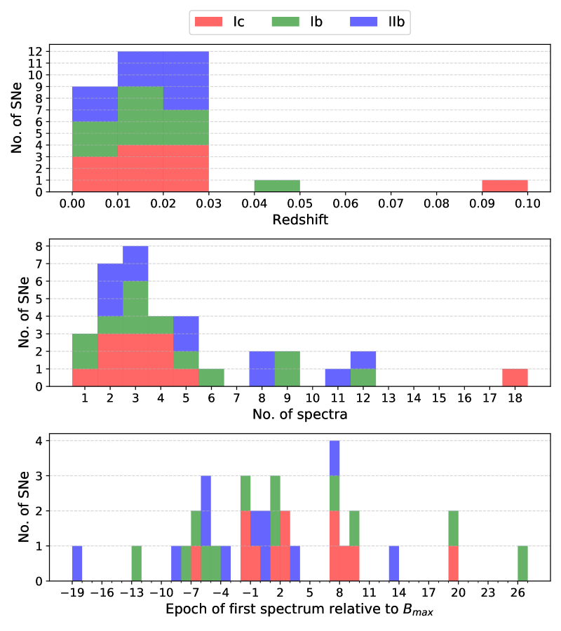
Figure 1: Breakdown of the sample. Top panel: Distribution of redshift ($z$) for the sample, as obtained from host-galaxy redshift measurements provided by the NASA/IPAC Extragalactic Database (NED). Middle panel: Distribution of the number of spectra per SN for the sample. Bottom panel: Temporal phase distribution of the first epoch of observation for the CSP-I SE SN spectroscopy sample.

The CSP-I carried out five, a nine-month-long observing campaigns between 2004 and 2009 centered on the southern hemisphere summer. By completion of the CSP-I, optical/NIR photometry and optical spectroscopy were obtained for several hundred SNe of all types, including 34 SE SNe largely discovered by targeted transient surveys (see Paper 1 for details). Table 1 contains a compilation of key information of each object as well as SN 2009dq which was not a part of the light curve sample presented in Paper 1. This includes: the Internationcal Astronomical Union (IAU) name, the coordinates, the redshift ($z$) of the host galaxy, the spectral classification, the number of spectra obtained for each object, the phase range of the spectra, and an estimate of the time of $t(B)_{max}$. Given our constraints to follow relatively bright SNe (i.e., peak apparent $m_{V}\leq 18$ mag) the targets are located in nearby galaxies. As demonstrated in the top panel of Fig. 1, 34 of the objects have heliocentric redshifts in the range $z=0.0046-0.0492$, while the luminous SN 2009ca (peak $M_{V}\approx-20$ mag) has a redshift of $z=0.0957$. Additional panels in Fig. 1 contain histograms of the number of spectra obtained per SN (middle panel) and the distribution of temporal phases with respect to $t(B)_{max}$ of the first epoch of observation (bottom panel).

The CSP-I spectroscopy sample of SE SNe was obtained with a handful of telescopes and instruments located in Chile. A journal of spectroscopic observations is provided in Table LABEL:table2. This includes a listing of the spectra, date of observations, the observational facilities, and the key spectral parameters: restframe phase relative to the epoch of $B$-band maximum, wavelength range, resolution, exposure time, and airmass. The vast majority of observations were conducted with facilities at the Las Campanas Observatory with the 2.5 m du Pont telescope and the 6.5 m Magellan Baade and Clay telescopes. Most of our spectra were taken with the du Pont telescope equipped with the Wide Field reimaging CCD (WFCCD) camera. A few spectra were also taken with the Boller & Chivens (B&C) spectrograph. Spectroscopy performed with the much larger-aperture Magellan telescopes made use of the Low Dispersion Survey Spectrograph 3 (LDSS3) and the Inamori Magellan Areal Camera and Spectrograph (IMACS). CSP-I also used the European Southern Observatory (ESO) 3.5 m New Technology Telescope (NTT) equipped with the ESO Multi-Mode Instrument (EMMI) and the 3.6 m telescope equipped with the ESO Faint Object Spectrograph and Camera (EFOSC), both located at the La Silla Observatory. In addition, the CSP-I also obtained three SE SN spectra with the Ritchey-Chrétien (RC) Cassegrain spectrograph attached the 1.5 m telescope at the Cerro Tololo Inter-American Observatory (CTIO), and a half dozen (mostly late phase) spectra with the Gemini Multi-Object Spectrograph (GMOS) attached to the 8.1 m Gemini-South telescope on Cerro Pachon.

The reduction procedures followed to obtain one-dimensional, flux-calibrated spectra are described in detail by Hamuy et al. (2006). In short, a two-dimensional spectral image is bias- and flat-field-corrected whereupon the SN trace is extracted. A wavelength calibration solution determined from arc lamp exposures is then applied to the one-dimensional extracted spectrum followed by (when possible) the division of a telluric spectrum. Next the wavelength-corrected (and telluric-corrected) one-dimensional spectrum is multiplied by a nightly sensitivity function determined from observations of one or more flux standard stars. If multiple science exposures are obtained for a given object on the same night, the one-dimensional spectra are averaged. Finally, prevalent cosmic rays are removed.

3 Results

3.1 Optical spectroscopy

The sample consists of 170 optical spectra of the 34 objects presented in Paper 1, as well as two spectra of the Type IIb SN 2009dq. The data sample covers a range of phases, extending from as early as $-$19 rest-frame days(d) relative to $t(B)_{max}$ (SN 2009K) to $+$310 d (SN 2008aq). The histograms plotted in the middle and bottom panels of Fig. 1 indicate that an average of two to three spectra were obtained per object and that for the majority of objects the first spectrum was obtained around the time of the $B$-band maximum. Four objects in the sample (i.e., SN 2007Y, SN 2008aq, SN 2009K and SN 2009bb) have a least one late-phase spectrum taken after $+$200 d. The nebular spectra of SN 2008aq and SN 2009K are presented for the first time and those of SN 2007Y and SN 2009bb were previously presented by Stritzinger et al. (2009) and Pignata et al. (2011), respectively. The final extracted, one-dimensional spectra, normalized to their mean flux values are plotted in Fig. 2. For presentation purposes, each plotted spectrum was smoothed using a median filter with a width of 5 pixels, while in a handful of objects widths of 7 pixels (SNe 2007kj and 2009dp) and 9 pixels (SNe 2006bf and SN 2006ep) were adopted.

To assess the general quality of the flux calibration of our SE SN spectroscopic sample, we compared the observed broadband colors of the SNe to the observed colors obtained from synthetic photometry. The inferred synthetic colors were computed for the entire WFCCD subset of spectra using the CSP-I system response functions that define the natural photometric system of the Swope telescope (see Stritzinger et al. 2011; Krisciunas et al. 2017).

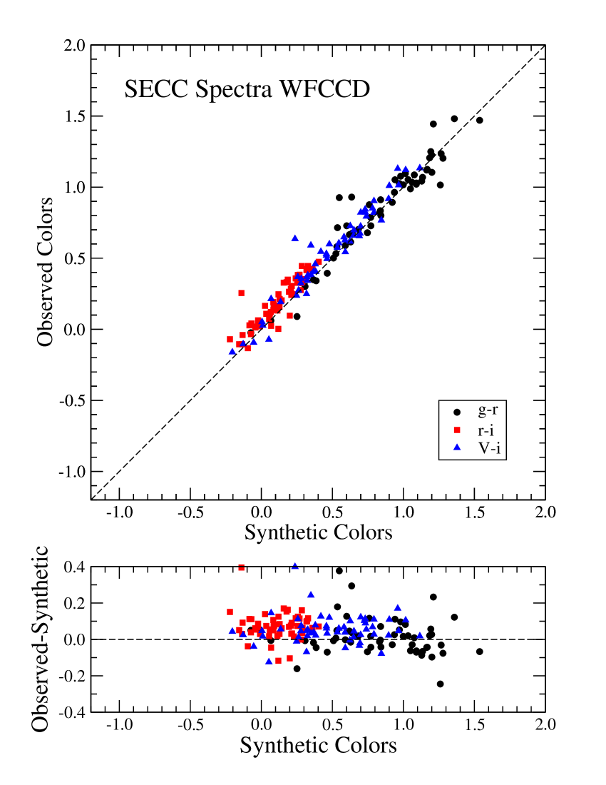
Figure 3: Quality of the spectral flux calibration. Top panel: Comparison between observed and synthetic colors ($g-r$) indicated with black dots, $(r-i$) with red squares, and ($V-i$) with blue triangles. Synthetic colors are computed using WFCCD spectra and the CSP-I system response functions (see Krisciunas et al. 2017, and references therein). Bottom panel: Residual between the observed and synthetic colors vs. synthetic colors. The dashed line has a slope of unity.

The results of this exercise are plotted in Fig. 3, which shows the comparisons between synthetic and observed ($g-r$), ($r-i$), and ($V-i$) colors in the top panel. In the bottom panel the differences between the observed and synthetic colors are plotted versus the corresponding synthetic colors. Comparison of the observed and synthetic colors reveals a fairly good agreement between the ($g-r$) colors, exhibiting average differences of $+0.015$ mag (with an associated root-mean-square uncertainty rms $=0.101$ mag). Good agreement is also found between the observed and synthetic ($V-r$) colors (not plotted in Fig. 3), which exhibit an average difference of $-0.017$ mag (rms of 0.059 mag).

Less agreement is found between the observed and synthetic colors that include the $i$ band. Specifically, the average difference between the observed versus synthetic ($V-i$) and ($r-i$) colors amounts to $+$0.055 mag (rms $=0.078$ mag) and $+$0.072 mag (rms $=0.073$ mag), respectively. The systematic offsets between the observed and synthetic ($V-i$) and ($r-i$) colors are evident in the bottom panel of Fig. 3. As a first step towards identifying the culprit of these offsets we eliminated spectra that contained prevalent telluric absorption. The curated sample provided improved ($V-i$) and ($r-i$) color offsets that decreased to $+$0.034 mag (rms $=0.064$ mag) and $+$0.055 mag (rms $=0.072$ mag), respectively. Although the offsets decreased, they are not entirely brought down to the levels found in the other color combinations that do not include the $i$ band.

We further investigated the issue and conducted an additional sequence of tests. First we examined whether poorly subtracted telluric absorption features could be a problem. To this end, observed and synthetic broadband colors were compared for the nearly dozen different spectrophotometric flux standards observed over the course of the CSP-I with the du Pont telescope equipped with WFCCD and which have had their telluric features removed following our standard procedures as prescribed by Bessell (1999). This test revealed average synthetic versus broadband color differences as follows: ($g-r$) $=+0.002$ mag (rms $=0.007$ mag), ($V-i$) $=+0.002$ mag (rms $=0.028$ mag), and ($r-i$) $=+0.006$ mag (rms $=0.024$ mag). The close agreement between these color indices reveals that, at least in the case of spectrophotometric standard star observations, our telluric removal technique produces robust results.

We also considered the accuracy of the CSP-I $i$-band system response function used to compute synthetic photometry as its measurement was not as robust as those of the other bands (Rheault et al. 2014). Indeed, the $i$-band system response function was only scanned a single time and suffered illumination issues at red wavelengths due to the light source used. To this end, synthetic colors were computed with the CSP-I system response functions using the atlas of spectrophotometric Landolt standard stars (Stritzinger et al. 2005), which have both Landolt (1992) and Smith et al. (2002) broadband photometry. Comparison between the resulting synthetic colors to those inferred from the broadband photometry of these stars yields average color differences as follows: ($g-r$) $=-0.005$ mag (rms $=0.010$ mag), ($V-i$) $=-0.031$ mag (rms $=0.018$ mag), and ($r-i$) $=-0.006$ mag (rms $=0.012$ mag).

Although we are unable to conclusively identify the culprit driving the offsets with the $i$-band colors, we speculate it is linked to the accuracy of the $i$-band system response function. Indeed, as noted by Rheault et al. (2014), the $i$-band system response function proved to be more difficult to measure and less accurate than the other bands due to the low illumination of the light source used in the scanning process. In summary, we find good agreement between the observed and synthetic colors that do not include the $i$ band.

3.2 Spectroscopic classification

We now turn to the spectral classification of objects in the CSP-I SE SN sample. If the spectrum of a given object lacked prevalent hydrogen and/or He i lines, we turned to guidance from the spectral template comparison program SNID (SuperNova IDentification; Blondin & Tonry 2007). In doing so, we made use of the expanded set of SE SN templates presented by Liu & Modjaz (2014). The spectroscopic classification of the sample is reported in Table 1 and reveals a breakdown between subtypes as follows: eleven SNe IIb, twelve SNe Ib, ten SNe Ic, and two SNe Ic-BL. As a caveat to these classifications, we note that traditionally it would not be entirely possible to exclude a SN IIb classification for the Type Ib SNe 2004ew, 2006ep, and 2008gc as their earliest spectra are post-maximum (see Table 1). However, as demonstrated in Paper 5, from pseudo-equivalent width measurements of certain spectral features and/or through the use of principal component analysis, these objects are confirmed to be SNe Ib. Similarly the distinction between some SNe Ib and SNe Ic is not always clear cut as was found in the cases of SNe 2005em and 2009dt, whose spectral phase coverage is limited to only good spectra taken around or before maximum (see Table 1). However, through the use of pEW measurements of O i and/or PCA these two objects are found to be consistent with a SN Ic classification.

In assigning classifications to SNe IIb no differentiation was made between objects thought to be characterized by extended or compact progenitors since such detailed subtyping is reliant on radio emission limits and/or detections (e.g., Chevalier & Soderberg 2010). In the case of SN 2009bb, previous papers by our group and collaborators have noted it exhibits broad spectral features akin to other SNe Ic-BL (Pignata et al. 2011) and that it displays signatures of a relativistic outflow possibly linked to a central engine (Soderberg et al. 2010). SN 2009ca is also a noteworthy object as its peak luminosity reached a value of at least $5\times 10^{43}$ ergs s^-1, which is reminiscent of SN 1992ar (Clocchiatti et al. 2000). This value is more than a factor of 10 larger compared to the average peak luminosity values determined from the literature sample of normal SNe Ic and a factor of 3 higher compared to the brightest of the gamma-ray bursts associated SNe Ic-BL, such as SN 2012bz (Schulze et al. 2014). Indeed, SN 2009ca appears to be a super-luminous supernova (see Taddia et al. 2018).

4 Summary

This paper presents 170 optical spectra of 35 SE SNe observed by CSP-I. The majority of the spectra were taken with facilities at the Las Campanas Observatory before or within a week after the epoch of $B$-band maximum. Nebular spectra are also presented for a subset of five objects. In general the spectra are of high quality and often cover the spectral range to around 9000 Å. In the companion paper presented by Holmbo et al. (2023, i.e., Paper 5) these data are used to construct mean template spectral sequences for the IIb, Ib, and Ic SE SN subtypes, study key line diagnostics, and perform a robust principle component analysis, leading to a fast and accurate method for classifying SE SN subtypes using only a single spectrum taken at either early or post-maximum epochs.

Table 1: Spectroscopic sample of CSP-I SE SNe.

SN	$\alpha(2000)$	$\delta(2000)$	Redshifta	Spectral	No. of	Phase	$t(B)_{\rm max}$
			$z$	Type	Spectra	Range	JD+2450000
2004ew	02:05:06.17	$-$55:06:31.6	0.0218	Ib	4	$+26\cdots+$81	$3276.11\pm 2.03$
2004ex	00:38:10.17	$+$02:43:16.9	0.0176	IIb	5	$-4\cdots+$41	$3306.69\pm 0.03$
2004fe	00:30:11.27	$+$02:05:23.5	0.0179	Ic	4	$+9\cdots+$35	$3316.79\pm 0.11$
2004ff	04:58:46.19	$-$21:34:12.0	0.0227	IIb	3	$+14\cdots+$30	$3312.60\pm 0.03$
2004gq	05:12:04.81	$-$15:40:54.2	0.0065	Ib	3	$-5\cdots+$24	$3357.90\pm 0.02$
2004gt	12:01:50.37	$-$18:52:12.7	0.0055	Ic	4	$-2\cdots+$49	$3360.37\pm 0.08$
2004gv	02:13:37.42	$-$00:43:05.8	0.0199	Ib	1	$-7\cdots-$7	$3365.27\pm 0.31$
2005Q	01:30:03.51	$-$42:40:48.4	0.0224	IIb	2	$-1\cdots+$7	$3406.10\pm 0.04$
2005aw	19:15:17.44	$-$54:08:24.9	0.0095	Ic	5	$+7\cdots+$23	$3456.48\pm 1.37$
2005bf	10:23:57.27	$-$03:11:28.6	0.0189	Ib	9	$-7\cdots+$52	$3474.79\pm 0.28$
2005bj	16:49:44.74	$+$17:51:48.7	0.0222	IIb	2	$+1\cdots+$4	$3471.89\pm 1.37$
2005em	03:13:47.71	$-$00:14:37.0	0.0260	Ic	1	$+0\cdots+$0	$3648.97\pm 1.36$
2006T	09:54:30.21	$-$25:42:29.3	0.0081	IIb	11	$+0\cdots+$70	$3779.61\pm 0.01$
2006ba	09:43:13.40	$-$09:36:53.0	0.0191	IIb	3	$+4\cdots+$28	$3820.92\pm 1.36$
2006bf	12:58:50.68	$+$09:39:30.1	0.0239	IIb	5	$+7\cdots$+33	$3817.46\pm 2.03$
2006ep	00:41:24.88	$+$25:29:46.7	0.0151	Ib	3	$+19\cdots+$34	$3985.41\pm 0.05$
2006fo	02:32:38.89	$+$00:37:03.0	0.0207	Ib	3	$+2\cdots+$18	$4003.17\pm 1.36$
2006ir	23:04:35.68	$+$07:36:21.5	0.0200	Ic	2	$+19\cdots+$43	$3999.07\pm 2.03$
2006lc	22:44:24.48	$-$00:09:53.5	0.0162	Ib	1	$+1\cdots+$1	$4041.33\pm 0.04$
2007C	13:08:49.30	$-$06:47:01.0	0.0056	Ib	9	$-1\cdots+$92	$4115.25\pm 1.37$
2007Y	03:02:35.92	$-$22:53:50.1	0.0046	Ib	12	$-12\cdots+$271	$4162.99\pm 0.01$
2007ag	10:01:35.99	$+$21:36:42.0	0.0207	Ib	2	$+7\cdots+$10	$4163.29\pm 1.42$
2007hn	21:02:46.85	$-$04:05:25.2	0.0273†	Ic	4	$+10\cdots+$56	$4351.63\pm 1.41$
2007kj	00:01:19.58	$+$13:06:30.6	0.0179	Ib	5	$-4\cdots+$40	$4380.91\pm 0.03$
2007rz	04:31:10.84	$+$07:37:51.5	0.0130	Ic	2	$+7\cdots+$32	$4437.31\pm 2.03$
2008aq	12:50:30.42	$-$10:52:01.4	0.0080	IIb	12	$-5\cdots+$308	$4531.15\pm 0.02$
2008gc	02:10:36.63	$-$53:45:59.5	0.0492†	Ib	6	$+9\cdots+$117	$4744.26\pm 1.37$
2008hh	01:26:03.65	$+$11:26:26.5	0.0194	Ic	3	$+2\cdots+$31	$4791.50\pm 2.03$
2009K	04:36:36.77	$-$00:08:35.6	0.0117	IIb	8	$-18\cdots+$282	$4867.22\pm 0.01$
2009Z	14:01:53.61	$-$01:20:30.2	0.0248	IIb	8	$-6\cdots+$41	$4876.94\pm 0.01$
2009bb	10:31:33.87	$-$39:57:30.0	0.0099	Ic-BL	18	$-1\cdots+$308	$4920.05\pm 0.02$
2009ca	21:26:22.20	$-$40:51:48.6	0.0957†	Ic-BL	3	$+3\cdots+$16	$4926.17\pm 2.03$
2009dp	20:26:52.69	$-$18:37:04.2	0.0232	Ic	3	$+2\cdots+$34	$4949.81\pm 2.03$
2009dq	10:08:49.94	$-$67:01:57.3	0.0047†	IIb	2	$-9\cdots+$14	$4960.50\pm 2.00$
2009dt	22:10:09.27	$-$36:05:42.6	0.0104	Ic	2	$-6\cdots-$16	$4958.31\pm 1.38$

$\begin{array}[]{cc}\includegraphics[width=195.12767pt]{SN2004ew.pdf}&\includegraphics[width=195.12767pt]{SN2004ex.pdf}\\ \includegraphics[width=195.12767pt]{SN2004fe.pdf}&\includegraphics[width=195.12767pt]{SN2004ff.pdf}\\ \end{array}$

Figure 2: Optical spectroscopy of the CSP-I SE SN sample. Each spectrum has been normalized to its mean flux values and plotted in units of $f_{\lambda}$. For presentation purposes additive constants have also been applied. The phase of each spectrum relative to the epoch of the $B$-band maximum is provided next to each spectrum and the spectroscopic subtype is provided below the SN designation at the top right. Vertical dashed blue lines indicate rest wavelengths of He i $\lambda\lambda$4472, 5876, 6678, 7065, 7281 lines, vertical dashed red lines are H$\gamma$, H$\beta$, and H$\alpha$, and the vertical gray line indicates the location of a prominent telluric feature.

$\begin{array}[]{cc}\includegraphics[width=195.12767pt]{SN2004gq.pdf}&\includegraphics[width=195.12767pt]{SN2004gt.pdf}\\ \includegraphics[width=195.12767pt]{SN2004gv.pdf}&\includegraphics[width=195.12767pt]{SN2005Q.pdf}\\ \end{array}$

Figure 2: Continued.

$\begin{array}[]{cc}\includegraphics[width=195.12767pt]{SN2005aw.pdf}&\includegraphics[width=195.12767pt]{SN2005bf.pdf}\\ \includegraphics[width=195.12767pt]{SN2005bj.pdf}&\includegraphics[width=195.12767pt]{SN2005em.pdf}\\ \end{array}$

Figure 2: Continued.

$\begin{array}[]{cc}\includegraphics[width=195.12767pt]{SN2006T.pdf}&\includegraphics[width=195.12767pt]{SN2006ba.pdf}\\ \includegraphics[width=195.12767pt]{SN2006bf.pdf}&\includegraphics[width=195.12767pt]{SN2006ep.pdf}\\ \end{array}$

Figure 2: Continued.

$\begin{array}[]{cc}\includegraphics[width=195.12767pt]{SN2006fo.pdf}&\includegraphics[width=195.12767pt]{SN2006ir.pdf}\\ \includegraphics[width=195.12767pt]{SN2006lc.pdf}&\includegraphics[width=195.12767pt]{SN2007C.pdf}\\ \end{array}$

Figure 2: Continued.

$\begin{array}[]{cc}\includegraphics[width=195.12767pt]{SN2007Y.pdf}&\includegraphics[width=195.12767pt]{SN2007ag.pdf}\\ \includegraphics[width=195.12767pt]{SN2007hn.pdf}&\includegraphics[width=195.12767pt]{SN2007kj.pdf}\\ \end{array}$

Figure 2: Continued.

$\begin{array}[]{cc}\includegraphics[width=195.12767pt]{SN2007rz.pdf}&\includegraphics[width=195.12767pt]{SN2008aq.pdf}\\ \includegraphics[width=195.12767pt]{SN2008gc.pdf}&\includegraphics[width=195.12767pt]{SN2008hh.pdf}\\ \end{array}$

Figure 2: Continued.

$\begin{array}[]{cc}\includegraphics[width=195.12767pt]{SN2009K.pdf}&\includegraphics[width=195.12767pt]{SN2009Z.pdf}\\ \includegraphics[width=195.12767pt]{SN2009bb.pdf}&\includegraphics[width=195.12767pt]{SN2009ca.pdf}\\ \end{array}$

Figure 2: Continued.

$\begin{array}[]{cc}\includegraphics[width=195.12767pt]{SN2009dp.pdf}&\includegraphics[width=195.12767pt]{SN2009dq.pdf}\\ \includegraphics[width=195.12767pt]{SN2009dt.pdf}\end{array}$

Figure 2: Continued.

Appendix A Journal of spectroscopic observations

Table 2: Journal of spectroscopic observations.

SN	UT Date	JD	Phase	Telescope	Instrument	Wavelength	Resolution	Exp. time	Airmass
		+2450000				Range [Å]	FWHM [Å]	[s]
2004ew	2004 Oct 24.22	3302.72	26.04	Clay	LDSS3	$3600-9000$	4.2	300	1.12
	2004 Nov 26.16	3335.66	58.28	Clay	LDSS3	$3600-9000$	4.2	300	1.15
	2004 Dec 13.14	3352.64	74.90	du Pont	WFCCD	$3800-9235$	3.0	900	1.20
	2004 Dec 19.04	3358.54	80.67	Clay	LDSS3	$3600-9000$	4.2	500	1.11
2004ex	2004 Oct 24.24	3302.74	$-$3.88	Clay	LDSS3	$3600-9000$	4.2	300	1.55
	2004 Nov 17.18	3326.68	19.65	du Pont	WFCCD	$3800-9235$	3.0	600	1.57
	2004 Nov 26.12	3335.62	28.43	Clay	LDSS3	$3600-9000$	4.2	300	1.35
	2004 Dec 04.09	3343.59	36.26	du Pont	WFCCD	$3800-9235$	3.0	900	1.28
	2004 Dec 09.09	3348.59	41.18	du Pont	WFCCD	$3800-9235$	3.0	900	1.35
2004fe	2004 Nov 16.06	3325.56	8.61	CTIO 1.5m	CS60	$3200-9617$	5.4	1200	1.18
	2004 Nov 17.14	3326.64	9.68	du Pont	WFCCD	$3800-9325$	3.1	600	1.32
	2004 Nov 26.10	3335.60	18.48	Clay	LDSS3	$3600-9000$	4.2	450	1.26
	2004 Dec 13.06	3352.56	35.14	du Pont	WFCCD	$3800-9235$	3.0	900	1.29
2004ff	2004 Nov 17.28	3326.78	13.86	du Pont	WFCCD	$3800-9235$	3.0	600	1.02
	2004 Nov 26.19	3335.69	22.57	Clay	LDSS3	$3600-9000$	4.2	450	1.03
	2004 Dec 04.22	3343.72	30.43	du Pont	WFCCD	$3800-9235$	3.0	600	1.01
2004gq	2004 Dec 13.23	3352.73	$-$5.13	du Pont	WFCCD	$3800-9235$	3.0	300	1.07
	2004 Dec 19.19	3358.69	0.78	Clay	LDSS3	$3600-9000$	4.2	180	1.03
	2005 Jan 11.16	3381.66	23.61	CTIO 1.5m	CS60	$3200-9615$	5.4	900	1.09
2004gt	2004 Dec 19.30	3358.80	$-$1.56	Clay	LDSS3	$3600-9000$	4.2	180	1.58
	2005 Jan 11.30	3381.80	21.31	CTIO 1.5m	CS60	$3200-9617$	5.4	1200	1.17
	2005 Feb 04.32	3405.82	45.20	du Pont	WFCCD	$3800-9235$	3.0	300	1.02
	2005 Feb 08.33	3409.83	49.19	du Pont	WFCCD	$3800-9235$	3.0	300	1.02
2004gv	2004 Dec 19.09	3358.59	$-$6.55	Clay	LDSS3	$3600-9000$	4.2	300	1.18
2005Q	2005 Feb 04.06	3405.56	$-$0.53	du Pont	WFCCD	$3800-9235$	3.0	400	1.58
	2005 Feb 12.05	3413.56	7.29	du Pont	WFCCD	$3800-9235$	3.0	400	1.76
2005aw	2005 Apr 03.33	3463.83	7.28	du Pont	WFCCD	$3800-9235$	3.0	500	1.39
	2005 Apr 07.39	3467.89	11.30	du Pont	WFCCD	$3800-9235$	3.0	600	1.16
	2005 Apr 12.40	3472.90	16.26	du Pont	WFCCD	$3800-9235$	3.0	500	1.13
	2005 Apr 15.39	3475.89	19.23	du Pont	WFCCD	$3800-9235$	3.0	500	1.13
	2005 Apr 19.40	3479.90	23.20	du Pont	WFCCD	$3800-9235$	3.0	500	1.11
2005bf	2005 Apr 07.07	3467.57	$-$7.08	du Pont	WFCCD	$3800-9235$	3.0	900	1.12
	2005 Apr 12.10	3472.60	$-$2.15	du Pont	WFCCD	$3800-9235$	3.0	900	1.12
	2005 Apr 15.13	3475.63	0.83	du Pont	WFCCD	$3800-9235$	3.0	900	1.20
	2005 Apr 19.01	3479.51	4.64	du Pont	WFCCD	$3800-9235$	3.0	700	1.15
	2005 May 06.97	3497.47	22.26	Clay	LDSS3	$3838-10000$	0.7	200	1.14
	2005 May 11.97	3502.47	27.17	Clay	LDSS3	$6057-10000$	1.1	900	1.12
	2005 May 31.16	3521.67	46.01	du Pont	WFCCD	$3800-8125$	3.0	1200	1.19
	2005 Jun 01.99	3523.49	47.79	du Pont	WFCCD	$3800-8128$	3.0	1200	1.16
	2005 Jun 06.04	3527.54	51.77	du Pont	WFCCD	$3800-8128$	3.0	600	1.48
2005bj	2005 Apr 12.35	3472.85	0.94	du Pont	WFCCD	$3800-9235$	$3.0$	$900$	1.47
	2005 Apr 15.35	3475.85	3.88	du Pont	WFCCD	$3800-9235$	$3.0$	$800$	1.48
2005em	2005 Oct 05.35	3648.85	$-$0.12	du Pont	WFCCD	$3800-9235$	$3.0$	$600$	1.21
2006T	2006 Feb 13.26	3779.76	0.15	ESO NTT	EMMI	$3200-10200$	$2.1$	$300$	1.03
	2006 Feb 27.35	3793.85	14.12	du Pont	WFCCD	$3800-9235$	$3.0$	$600$	1.72
	2006 Mar 05.22	3799.72	19.95	du Pont	WFCCD	$3800-9235$	$3.0$	$600$	1.06
	2006 Mar 08.23	3802.73	22.93	du Pont	WFCCD	$3800-9235$	$3.0$	$900$	1.09
	2006 Mar 14.21	3808.71	28.86	Clay	LDSS3	$3785-9972$	$1.2$	$400$	1.14
	2006 Mar 22.19	3816.69	36.78	du Pont	WFCCD	$3800-9235$	$3.0$	$900$	1.09
	2006 Mar 24.15	3818.65	38.73	du Pont	WFCCD	$3800-9235$	$3.0$	$900$	1.03
	2006 Apr 02.10	3827.60	47.61	du Pont	WFCCD	$3800-9235$	$3.0$	$900$	1.01
	2006 Apr 16.24	3841.74	61.63	Baade	IMACS	$3842-9692$	$2.0$	$600$	2.09
	2006 Apr 23.10	3848.60	68.43	du Pont	WFCCD	$3800-9235$	$3.0$	$900$	1.08
	2006 Apr 25.05	3850.55	70.73	du Pont	WFCCD	$3800-9235$	$3.0$	$900$	1.02
2006ba	2006 Mar 30.15	3824.65	3.66	du Pont	WFCCD	$3800-9235$	$3.0$	$900$	1.13
	2006 Apr 16.07	3841.57	20.27	Baade	IMACS	$3842-9692$	$2.0$	$900$	1.08
	2006 Apr 24.04	3849.54	28.08	du Pont	WFCCD	$3800-9235$	$3.0$	$900$	1.07
2006bf	2006 Mar 30.31	3824.81	7.18	du Pont	WFCCD	$3800-9235$	$3.0$	$900$	1.54
	2006 Apr 02.32	3827.82	10.12	du Pont	WFCCD	$3800-9235$	$3.0$	$1200$	1.67
	2006 Apr 22.25	3847.75	29.58	du Pont	WFCCD	$3800-9235$	$3.0$	$1000$	1.53
	2006 Apr 23.23	3848.73	30.54	du Pont	WFCCD	$3800-9235$	$3.0$	$1000$	1.47
	2006 Apr 25.28	3850.78	32.55	du Pont	WFCCD	$3800-9235$	$3.0$	$900$	2.04
2006ep	2006 Sep 26.20	4004.70	19.00	du Pont	WFCCD	$3800-9235$	$3.0$	$1200$	1.74
	2006 Oct 10.19	4018.69	32.79	du Pont	WFCCD	$3800-9235$	$3.0$	$1200$	1.74
	2006 Oct 11.18	4019.68	33.76	du Pont	WFCCD	$3800-9235$	$3.0$	$1200$	1.73
2006fo	2006 Sep 26.28	4004.78	1.58	du Pont	WFCCD	$3800-9235$	$3.0$	$1200$	1.16
	2006 Sep 28.26	4006.76	3.52	du Pont	WFCCD	$3800-9235$	$3.0$	$1200$	1.18
	2006 Oct 13.32	4021.82	18.27	du Pont	WFCCD	$3800-9235$	$3.0$	$1200$	1.28
2006ir	2006 Oct 10.10	4018.60	19.14	du Pont	WFCCD	$3800-9235$	$3.0$	$600$	1.25
	2006 Nov 03.14	4042.64	42.71	ESO NTT	EMMI	$4012-10200$	$3.3$	$300$	1.53
2006lc	2006 Nov 03.08	4042.58	1.23	ESO NTT	EMMI	$3200-10200$	$2.1$	$300$	1.20
2007C	2007 Jan 13.34	4113.84	$-$1.40	du Pont	B&C	$3932-10142$	$3.0$	$300$	1.29
	2007 Jan 18.28	4118.78	3.51	du Pont	B&C	$3402-9614$	$3.0$	$900$	1.63
	2007 Jan 31.36	4131.86	16.52	ESO NTT	EMMI	$3200-5300$	$2.1$	$400$	1.10
	2007 Feb 12.37	4143.87	28.46	du Pont	WFCCD	$3800-9235$	$3.0$	$400$	1.09
	2007 Feb 19.38	4150.88	35.43	du Pont	WFCCD	$3800-9235$	$3.0$	$400$	1.13
	2007 Feb 25.35	4156.85	41.37	du Pont	WFCCD	$3800-9235$	$3.0$	$400$	1.10
	2007 Mar 04.27	4163.77	48.25	ESO NTT	EMMI	$4000-10200$	$3.3$	$300$	1.09
	2007 Mar 19.22	4178.72	63.12	du Pont	B&C	$3419-9626$	$3.0$	$900$	1.11
	2007 Apr 17.30	4207.80	92.04	du Pont	WFCCD	$3800-9235$	$3.0$	$600$	1.51
2007Y	2007 Feb 19.04	4150.54	$-$12.39	du Pont	WFCCD	$3800-9235$	$3.0$	$600$	1.31
	2007 Feb 25.02	4156.52	$-$6.44	du Pont	WFCCD	$3800-9235$	$3.0$	$600$	1.28
	2007 Mar 04.05	4163.55	0.56	ESO NTT	EMMI	$3200-10200$	$2.1$	$200$	1.76
	2007 Mar 11.00	4170.50	7.47	Baade	IMACS	$3789-10879$	$2.0$	$600$	1.42
	2007 Mar 14.01	4173.51	10.47	du Pont	B&C	$3429-9648$	$3.0$	$600$	1.62
	2007 Mar 19.00	4178.50	15.44	du Pont	B&C	$3419-9631$	$3.0$	$600$	1.60
	2007 Mar 25.99	4185.49	22.39	du Pont	B&C	$3400-9606$	$3.0$	$600$	1.73
	2007 Apr 12.98	4203.48	40.30	du Pont	WFCCD	$3800-9235$	$3.0$	$800$	2.59
	2007 Oct 21.32	4394.82	230.76	Clay	LDSS3	$4097-9979$	$0.7$	$900$	1.11
	2007 Oct 23.30	4396.80	232.73	Clay	LDSS3	$4033-9988$	$0.7$	$1200$	1.06
	2007 Nov 17.28	4421.78	257.60	Baade	IMACS	$3809-10675$	$2.0$	$1800$	1.21
	2007 Dec 01.21	4435.71	271.46	ESO 3.6m	EFOSC	$3300-9260$	$2.8$	$1200$	1.09
2007ag	2007 Mar 11.17	4170.67	7.23	Baade	IMACS	$3789-10887$	$2.0$	$600$	1.59
	2007 Mar 14.13	4173.63	10.13	du Pont	B&C	$3429-9642$	$3.0$	$1200$	1.15
2007hn	2007 Sep 18.20	4361.70	9.80	du Pont	B&C	$3408-9614$	$3.0$	$1200$	1.43
	2007 Oct 04.03	4377.53	25.21	ESO 3.6m	EFOSC	$3300-9260$	$2.8$	$1200$	1.11
	2007 Oct 05.05	4378.55	26.20	Clay	LDSS3	$4452-9303$	$2.0$	$1200$	1.10
	2007 Nov 05.01	4409.51	56.34	ESO 3.6m	EFOSC	$3300-9260$	$2.7$	$1200$	1.16
2007kj	2007 Oct 03.15	4376.65	$-$4.18	ESO 3.6m	EFOSC	$3300-9260$	$2.8$	$600$	1.36
	2007 Oct 05.12	4378.63	$-$2.24	Clay	LDSS3	$4452-9303$	$2.0$	$600$	1.39
	2007 Oct 16.18	4389.68	8.61	du Pont	B&C	$3412-9624$	$3.0$	$900$	1.40
	2007 Oct 21.13	4394.63	13.48	du Pont	B&C	$3352-9563$	$3.0$	$1200$	1.35
	2007 Nov 17.10	4421.60	39.98	Baade	IMACS	$3809-10675$	$2.0$	$600$	1.46
2007rz	2007 Dec 10.26	4444.76	7.35	du Pont	WFCCD	$3800-9235$	$3.0$	$700$	1.48
	2008 Jan 04.12	4469.62	31.89	ESO 3.6m	EFOSC	$3300-9260$	$2.8$	$600$	1.26
2008aq	2008 Feb 29.31	4525.81	$-$5.30	Baade	IMACS	$3743-10721$	$2.0$	$600$	1.06
	2008 Mar 14.32	4539.82	8.60	ESO 3.6m	EFOSC	$3300-9240$	$2.7$	$600$	1.12
	2008 Mar 19.31	4544.81	13.55	Clay	MagE	$3101-9344$	$0.3$	$1200$	1.13
	2008 Mar 20.32	4545.82	14.55	Clay	LDSS3	$3629-9437$	$2.0$	$600$	1.19
	2008 Mar 28.33	4553.83	22.50	ESO NTT	EMMI	$3200-10200$	$2.1$	$300$	1.35
	2008 Mar 31.29	4556.79	25.43	du Pont	WFCCD	$3800-9235$	$3.0$	$600$	1.18
	2008 Apr 12.27	4568.77	37.33	du Pont	WFCCD	$3800-9235$	$3.0$	$600$	1.26
	2008 Apr 26.22	4582.72	51.16	Baade	IMACS	$4246-10374$	$2.0$	$600$	1.17
	2008 Apr 29.19	4585.69	54.11	du Pont	WFCCD	$3800-9235$	$3.0$	$600$	1.13
	2008 May 11.15	4597.65	65.98	du Pont	WFCCD	$3800-9235$	$3.0$	$600$	1.12
	2008 May 22.15	4608.65	76.89	Baade	IMACS	$4338-10868$	$2.0$	$600$	1.19
	2009 Jan 10.28	4841.78	308.17	Gemini-S	GMOS	$3900-8118$	$1.4$	$1800$	1.53
2008gc	2008 Oct 14.32	4753.82	9.11	ESO NTT	EFOSC	$3401-9210$	$2.8$	$1200$	1.26
	2008 Oct 15.15	4754.65	9.90	ESO NTT	EFOSC	$3351-9210$	$2.7$	$1200$	1.17
	2008 Oct 20.22	4759.72	14.74	du Pont	WFCCD	$3800-9235$	$3.0$	$900$	1.10
	2008 Oct 28.30	4767.80	22.43	du Pont	WFCCD	$3800-9235$	$3.0$	$1200$	1.25
	2008 Nov 04.07	4774.57	28.89	Clay	LDSS3	$3636-9452$	$2.0$	$1000$	1.23
	2009 Jan 30.04	4861.54	117.28	Gemini-S	GMOS	$3902-8118$	$1.4$	$2400$	1.32
2008hh	2008 Nov 23.12	4793.62	2.08	du Pont	WFCCD	$3800-9235$	$3.0$	$600$	1.36
	2008 Dec 08.10	4808.60	16.78	Baade	IMACS	$4023-10719$	$2.0$	$900$	1.41
	2008 Dec 23.04	4823.54	31.43	du Pont	WFCCD	$3800-9235$	$3.0$	$1200$	1.35
2009K	2009 Jan 17.09	4848.59	$-$18.42	Clay	LDSS3	$3629-9440$	$2.0$	$500$	1.15
	2009 Jan 22.08	4853.58	$-$13.48	Clay	LDSS3	$3620-9428$	$2.0$	$300$	1.16
	2009 Feb 08.13	4870.63	3.37	Clay	LDSS3	$3716-9438$	$2.0$	$500$	1.59
	2009 Feb 11.07	4873.57	6.28	Baade	IMACS	$4032-10122$	$2.0$	$500$	1.27
	2009 Feb 25.08	4887.58	20.13	du Pont	WFCCD	$3800-9235$	$3.0$	$500$	1.61
	2009 Mar 16.00	4906.50	38.83	ESO NTT	EFOSC	$3300-9210$	$2.7$	$500$	1.57
	2009 Mar 28.02	4918.53	50.71	du Pont	WFCCD	$3800-9235$	$3.0$	$500$	1.93
	2009 Nov 17.33	5152.84	282.31	Gemini-S	GMOS	$4099-7999$	$1.4$	$1350$	1.50
2009Z	2009 Feb 08.35	4870.85	$-$5.95	Clay	LDSS3	$3716-9439$	$2.0$	$900$	1.20
	2009 Feb 11.35	4873.85	$-$3.01	Baade	IMACS	$4032-10120$	$2.0$	$800$	1.17
	2009 Feb 15.37	4877.87	0.91	Baade	IMACS	$4021-10121$	$2.0$	$600$	1.13
	2009 Feb 24.35	4886.85	9.67	du Pont	WFCCD	$3800-9235$	$3.0$	$700$	1.13
	2009 Feb 25.31	4887.81	10.61	du Pont	WFCCD	$3800-9235$	$3.0$	$900$	1.18
	2009 Feb 26.37	4888.87	11.65	du Pont	WFCCD	$3800-9235$	$3.0$	$900$	1.14
	2009 Mar 15.36	4905.86	28.22	Baade	IMACS	$4026-10114$	$2.0$	$900$	1.20
	2009 Mar 28.37	4918.87	40.92	du Pont	WFCCD	$3800-9235$	$3.0$	$900$	1.41
2009bb	2009 Mar 28.19	4918.69	$-$1.35	du Pont	WFCCD	$3800-9235$	$3.0$	$700$	1.09
	2009 Mar 29.10	4919.60	$-$0.45	du Pont	WFCCD	$3800-9235$	$3.0$	$900$	1.03
	2009 Apr 03.14	4924.64	4.55	du Pont	WFCCD	$3800-9235$	$3.0$	$700$	1.04
	2009 Apr 07.00	4928.50	8.37	Baade	IMACS	$4057-10139$	$2.0$	$400$	1.16
	2009 Apr 15.31	4936.81	16.60	Gemini-S	GMOS	$3904-8122$	$1.4$	$900$	1.03
	2009 Apr 17.10	4938.60	18.37	Clay	LDSS3	$3714-9435$	$2.0$	$600$	1.03
	2009 Apr 18.08	4939.58	19.34	du Pont	B&C	$3450-9657$	$3.0$	$700$	1.02
	2009 Apr 22.08	4943.58	23.30	du Pont	B&C	$3360-9567$	$3.0$	$900$	1.03
	2009 Apr 23.11	4944.61	24.32	du Pont	B&C	$3362-9565$	$3.0$	$1000$	1.07
	2009 Apr 26.31	4947.81	27.49	Gemini-S	GMOS	$3904-8122$	$1.4$	$900$	1.03
	2009 Apr 30.13	4951.64	31.28	Clay	LDSS3	$3702-9443$	$2.0$	$600$	1.18
	2009 May 01.08	4952.58	32.21	Clay	LDSS3	$3721-9445$	$2.0$	$600$	1.05
	2009 May 14.03	4965.53	45.04	Baade	IMACS	$3974-10136$	$2.0$	$600$	1.04
	2009 May 22.96	4974.46	53.88	du Pont	B&C	$3360-9565$	$3.0$	$900$	1.02
	2009 May 31.05	4982.55	61.89	du Pont	B&C	$3394-9591$	$3.0$	$1200$	1.17
	2010 Jan 09.21	5205.71	282.86	Clay	LDSS3	$3632-9441$	$2.0$	$1800$	1.33
	2010 Jan 10.29	5206.79	283.93	Gemini-S	GMOS	$4197-8424$	$1.4$	$4000$	1.02
	2010 Feb 03.09	5230.59	307.50	Baade	IMACS	$3975-10051$	$2.0$	$1800$	1.75
2009ca	2009 Apr 07.42	4928.92	2.51	Baade	IMACS	$4057-10139$	$2.0$	$900$	1.31
	2009 Apr 17.35	4938.85	11.57	Clay	LDSS3	$3714-9435$	$2.0$	$700$	1.62
	2009 Apr 22.37	4943.87	16.15	du Pont	B&C	$3360-9567$	$3.0$	$900$	1.36
2009dp	2009 Apr 30.33	4951.83	1.98	Clay	LDSS3	$3702-9445$	$2.0$	$600$	1.28
	2009 May 01.37	4952.87	2.99	Clay	LDSS3	$3721-9445$	$2.0$	$600$	1.11
	2009 Jun 02.28	4984.78	34.18	Clay	MagE	$3181-9111$	$0.2$	$900$	1.12
2009dq	2009 Apr 30.10	4951.60	$-$8.85	Clay	LDSS3	$3702-9422$	$2.0$	$400$	1.36
	2009 May 23.05	4974.55	13.98	du Pont	B&C	$3360-9563$	$3.0$	$600$	1.37
2009dt	2009 Apr 30.36	4951.86	$-$6.38	Clay	LDSS3	$3702-9445$	$2.0$	$600$	1.44
	2009 May 23.39	4974.89	16.41	du Pont	B&C	$3360-9565$	$3.0$	$900$	1.06

Table 2: continued