Distributional Learning of Variational AutoEncoder: Application to Synthetic Data Generation

Abstract

The Gaussianity assumption has been consistently criticized as a main limitation of the Variational Autoencoder (VAE) despite its efficiency in computational modeling. In this paper, we propose a new approach that expands the model capacity (i.e., expressive power of distributional family) without sacrificing the computational advantages of the VAE framework. Our VAE model’s decoder is composed of an infinite mixture of asymmetric Laplace distribution, which possesses general distribution fitting capabilities for continuous variables. Our model is represented by a special form of a nonparametric M-estimator for estimating general quantile functions, and we theoretically establish the relevance between the proposed model and quantile estimation. We apply the proposed model to synthetic data generation, and particularly, our model demonstrates superiority in easily adjusting the level of data privacy.

1 Introduction

Variational Autoencoder (VAE) [31, 51] and Generative Adversarial Networks (GAN) [22] are generative models that are used to estimate the underlying distribution of a given dataset. To avoid the curse of dimensionality, VAE and GAN commonly introduce a low-dimensional latent space on which a conditional generative model is defined. By minimizing an information divergence between the original data and its generated data, the generative models are learned to produce synthetic data similar to the original one. Accordingly, VAE and GAN have been applied in various applications, such as generating realistic images, texts, and synthetic tabular data for privacy preservation purposes [30, 60, 63, 65, 34].

However, the difference in the strength of the assumption about the generative distribution brings significant contrasts in the VAE and GAN generation performances [30, 7, 17]. In the GAN framework, the adversarial loss enables direct minimization of the Jensen-Shannon divergence between the ground-truth density function and the generative distribution under no distributional assumption [13, 59]. Roughly speaking, the GAN employs a nonparametric model as its conditional generative model defined on the latent space.

On the contrary, in the VAE framework, the Gaussianity assumption has been favored [31, 32, 15, 10, 39]. It is because Gaussianity gives us three advantages: 1) the reconstruction loss can be interpreted as the mean squared error that is one of the most popular losses in optimization theory, 2) generating a new sample is computationally straightforward, and 3) KL-divergence is computed in a simple closed form. However, these benefits have led us to pay the price for the distributional capacity of the generative model, in that the generative model of the VAE is constrained in the form of marginalization of the product of the two Gaussian distributions. Here, the distributional capacity means the expressive power of the distributional family. This restricted distributional capacity has been the critical limitation [8, 33] and leads to a heavy parameterization of the decoder mean vector to approximate complex underlying distributions.

To increase the distributional capacity in synthetic data generation, [63, 65] introduce the multi-modality in the distributional assumption of the decoder, which is known as the mode-specific normalization technique. Although the mixture Gaussian decoder modeling of [63, 65] allows handling more complex distributions of the observed dataset while preserving all of the advantages of Gaussianity, we numerically find that the mixture Gaussian is not enough to capture the complex underlying distribution.

Our main contribution is that, beyond Gaussianity, we propose a novel VAE learning method that directly estimates the conditional cumulative distribution function (CDF) while maintaining the objective of maximizing the Evidence Lower Bound (ELBO) of the observed dataset. It implies that we have a nonparametric distribution assumption on the generative model. We call this approach distributional learning of the VAE, which is enabled by estimating an infinite number of conditional quantiles [4, 20]. By adopting the continuous ranked probability score (CRPS) loss, the objective function of our proposed distribution learning method is computationally tractable [21, 43, 20].

In our proposed distributional learning framework, 1) the reconstruction loss is equivalent to the CRPS loss, which is a proper scoring rule [21, 43], 2) generating a new sample is still computationally straightforward due to the inverse transform sampling, and 3) KL-divergence is still computed in a simple closed form. To show the effectiveness of our proposed model in capturing the underlying distribution of the dataset, we evaluate our model for synthetic data generation with real tabular datasets.

2 Related Work

Modeling of the decoder and reconstruction loss. To increase the distributional capacity, many papers have focused on decoder modeling while not losing the mathematical link to maximize the ELBO. [57, 1] assume their decoder distributions as Student-$t$ and asymmetric Laplace distributions, respectively, to mitigate the zero-variance problem that the model training becomes unstable if the estimated variance of the decoder shrinks to zero in Gaussian VAE [41, 55, 15]. [2] proposes a general distribution of the decoder, which allows improved robustness by optimizing the shape of the loss function during training. Recently, [5] proposes a reconstruction loss that directly minimizes the blur error of the VAE by modeling the covariance matrix of multivariate Gaussian decoder.

On the other hand, there exists a research direction that focuses on replacing the reconstruction loss without concern for losing the mathematical derivation of the lower bound. [38, 52, 46] replace the reconstruction loss with an adversarial loss of the GAN framework. [27] introduces a feature-based loss that is calculated with a pre-trained convolutional neural network (CNN). Another approach by [14] adopts Watson’s perceptual model, and [28] directly optimizes the generative model in the frequency domain by a focal frequency reconstruction loss. Most of the above-mentioned methods aim to capture the properties of human perception by replacing the element-wise loss ($L_{1}$ or $L_{2}$-norm), which hinders the reconstruction of images [38].

Synthetic data generation. The GAN framework is widely adopted in the synthetic data generation task since it enables synthetic data generation in a nonparametric approach [12, 47, 63, 65]. [63, 65] assume that continuous columns of tabular datasets can be approximated by the Gaussian mixture distribution and model their decoder using Gaussian mixture distribution. Additionally, [63, 65] preprocess the continuous variables using the variational Gaussian mixture model [3], which is known as the mode-specific normalization technique. However, the preprocessing step requires additional computational resources and hyperparameter tuning of the number of modes. Other approaches by [47, 65] regularize the discrepancy between the first and second-order statistics of the observed and synthetic dataset. [12] proposes the GAN-based synthesizer, which focuses on generating high-dimensional discrete variables with the assistance of the pre-trained AutoEncoder.

3 Proposal

Let ${\bf x}\in\mathbb{R}^{p+q}$ be an observation consisting of continuous and discrete variables and $I=I_{C}\cup I_{D}=\{1,\cdots,(p+q)\}$ be an index set of the variables, where $I_{C}$ and $I_{D}$ correspond to index sets of $p$ continuous and $q$ discrete variables. $T_{j}$ denotes the number of levels for the discrete variables ${\bf x}_{j},j\in I_{D}$. We denote the ground-truth underlying distribution (probability density function, PDF) as $p({\bf x})$ and the ground-truth CDF as $F({\bf x})$.

Let ${\bf z}$ be a latent variable, where ${\bf z}\in\mathbb{R}^{d}$ and $d<p+q$. The prior and posterior distribution of ${\bf z}$ are assumed to be $p({\bf z})=\mathcal{N}({\bf z}|\mathbf{0},\mathbf{I})$ and $q({\bf z}|{\bf x};\phi)=\mathcal{N}\big{(}{\bf z}|\mu({\bf x};\phi),diag(\sigma^{2}({\bf x};\phi))\big{)}$, respectively. Here, $\mathbf{I}$ is $d\times d$ identity matrix, $\mu:\mathbb{R}^{p+q}\mapsto\mathbb{R}^{d}$, $\sigma^{2}:\mathbb{R}^{p+q}\mapsto\mathbb{R}_{+}^{d}$ are neural networks parameterized with $\phi$, and $diag(a),a\in\mathbb{R}^{d}$ denotes a diagonal matrix with diagonal elements $a$. Moreover, we consider $\alpha\in[0,1]$ as a random variable having density $p(\alpha)$.

3.1 Distributional Learning

Our proposed model assumes that $p({\bf x})$ is parametrized by an infinite mixture of asymmetric Laplace distribution (ALD) [4]. The ALD is characterized by two parameters: $\alpha$, representing the asymmetry, and $\beta>0$, representing the scale. By considering these parameters, along with the model parameter $\theta$, we can define the probability model of ${\bf x}$ as follows:

$$p({\bf x};\theta,\beta)=\int\int_{0}^{1}p({\bf x}|{\bf z},\alpha;\theta,\beta)p({\bf z},\alpha)d\alpha d{\bf z}.$$

Assumption 1.

(1) $\{{\bf x}_{j}\}_{j\in I}$ are conditionally independent given ${\bf z}$. (2) The discrete random variables $\{{\bf x}_{j}\}_{j\in I_{D}}$ are independent of $\alpha$. (3) $\alpha$ and ${\bf z}$ are independent.

By Assumption 1-(1), we model the dependency between ${\bf x}_{j}$s solely through the latent variable ${\bf z}$ [49]. Assumption 1-(2) implies that $\alpha$ is related only to the continuous variables. Then, the decoder of our VAE model denoted as $p({\bf x}|{\bf z},\alpha;\theta,\beta)$ is specified by equation (3.1):

$$p({\bf x}|{\bf z},\alpha;\theta,\beta) = \prod_{j\in I_{C}}p({\bf x}_{j}|{\bf z},\alpha;\theta_{j},\beta)\cdot\prod_{j\in I_{D}}p({\bf x}_{j}|{\bf z};\theta_{j})$$

$$= \prod_{j\in I_{C}}\frac{\alpha(1-\alpha)}{\beta}\exp\left(-\rho_{\alpha}\left(\frac{{\bf x}_{j}-D_{j}(\alpha,{\bf z};\theta_{j})}{\beta}\right)\right)\cdot\prod_{j\in I_{D}}\prod_{l=1}^{T_{j}}\pi_{l}({\bf z};\theta_{j})^{\mathbb{I}({\bf x}_{j}=l)},$$

where $\theta=(\theta_{1},\cdots,\theta_{p+q})$, $\beta$ is a non-trainable constant, $\rho_{v}(u)=u(v-\mathbb{I}(u<0))$ (check function), and $\mathbb{I}(\cdot)$ denotes the indicator function. $D_{j}(\cdot,\cdot;\theta_{j}):[0,1]\times\mathbb{R}^{d}\mapsto\mathbb{R}$ is the location parameter of ALD, which is parameterized with $\theta_{j}$ [1]. For discrete variables, $\pi(\cdot;\theta_{j}):\mathbb{R}^{d}\mapsto\Delta^{T_{j}-1}$ is a neural network parameterized with $\theta_{j}$, where $\Delta^{T_{j}-1}$ is the standard $(T_{j}-1)$-simplex for all ${\bf z}\in\mathbb{R}^{d}$, and the subscript $l$ referes to the $l$th element of the output $\pi$.

Assumption 1-(3) leads our objective function,

$$\min_{\theta,\phi} \mathbb{E}_{p({\bf x})}\mathbb{E}_{q({\bf z}|{\bf x};\phi)}\left[\sum_{j\in I_{C}}\int_{0}^{1}\rho_{\alpha}\Big{(}{\bf x}_{j}-D_{j}(\alpha,{\bf z};\theta_{j})\Big{)}d\alpha-\sum_{j\in I_{D}}\sum_{l=1}^{T_{j}}\mathbb{I}({\bf x}_{j}=l)\cdot\log\pi_{l}({\bf z};\theta_{j})\right]$$ (2)

$$+ \beta\cdot\mathbb{E}_{p({\bf x})}[\mathcal{KL}(q({\bf z}|{\bf x};\phi)\|p({\bf z}))],$$

where constant terms are omitted. In order to achieve balanced learning of the two reconstruction losses in (2), we have removed the weight $\beta$ associated with the second reconstruction loss. We refer to our model as ‘DistVAE.’ The first term in (2) corresponds to the CRPS loss, which measures the accuracy of the proposed CDF approximation with respect to the ground-truth CDF of the underlying distribution [21, 43, 20].

Interestingly, (2) is the limit of the negative ELBO derived from a finite mixture of ALD. We introduce $\alpha$, a discrete uniform random variable taking values on $\alpha_{k}=k/K$ for $k=1,\cdots,K$. Then, the negative ELBO of $p({\bf x};\theta,\beta)$ scaled with $\beta$ is written by

$$\mathbb{E}_{q({\bf z}|{\bf x};\phi)}\left[\sum_{j\in I_{C}}\frac{1}{K}\sum_{k=1}^{K}\rho_{\alpha_{k}}\Big{(}{\bf x}_{j}-D_{j}(\alpha_{k},{\bf z};\theta_{j})\Big{)}\right]-\beta\frac{p}{K}\sum_{k=1}^{K}\log\alpha_{k}(1-\alpha_{k})+\beta p\log\beta$$ (3)

$$- \beta\cdot\mathbb{E}_{q({\bf z}|{\bf x};\phi)}\left[\sum_{j\in I_{D}}\sum_{l=1}^{T_{j}}\mathbb{I}({\bf x}_{j}=l)\cdot\log\pi_{l}({\bf z};\theta_{j})\right]+\beta\cdot\mathcal{KL}(q({\bf z}|{\bf x};\phi)\|p({\bf z}))$$

(see Appendix A.1 for detailed derivation). The reconstruction loss, which corresponds to the first term of (3), is a composite quantile loss for estimating the target quantiles $\alpha_{k}$s [64, 35, 45, 62, 9]. This entails adopting a Bayesian perspective for $\alpha$ as a prior (the Bayesian modeling for estimating multiple quantiles). Furthermore, throughout the derivation of the reconstruction loss, the role of $\alpha$ is pivotal in ensuring the representation of the reconstruction loss. To prevent the observation ${\bf x}$ from influencing the distribution of $\alpha$, $\alpha$ is only assigned with a prior distribution, and the resulting reconstruction loss becomes the CRPS loss, a proper scoring rule.

However, for distributional learning of VAE, it is necessary to estimate conditional quantiles for an infinite number of quantile levels, denoted by $K\rightarrow\infty$ [50]. The subsequent Theorem 1 establishes the convergence of the negative ELBO (3) to our objective function (2) as $K\rightarrow\infty$ [4].

Theorem 1.

For all $j\in I_{C}$, suppose that $\int_{0}^{1}\mathbb{E}_{p({\bf x})}\mathbb{E}_{q({\bf z}|{\bf x};\phi)}\rho_{\alpha}\big{(}{\bf x}_{j}-D_{j}(\alpha,{\bf z};\theta_{j})\big{)}d\alpha<\infty$, and $\mathbb{E}_{p({\bf x})}\mathbb{E}_{q({\bf z}|{\bf x};\phi)}[\rho_{\alpha}({\bf x}_{j}-D_{j}(\alpha,{\bf z};\theta_{j}))]$ is continuous over $\alpha\in(0,1)$. Then,

$$\lim_{K\rightarrow\infty}\mathbb{E}_{p({\bf x})}\mathbb{E}_{q({\bf z}|{\bf x};\phi)}\left[\frac{1}{K}\sum_{k=1}^{K}\rho_{\alpha_{k}}\Big{(}{\bf x}_{j}-D_{j}(\alpha_{k},{\bf z};\theta_{j})\Big{)}\right]=\mathbb{E}_{p({\bf x})}\mathbb{E}_{q({\bf z}|{\bf x};\phi)}\left[\int_{0}^{1}\rho_{\alpha}\Big{(}{\bf x}_{j}-D_{j}(\alpha,{\bf z};\theta_{j})\Big{)}d\alpha\right],$$

and $\lim_{K\rightarrow\infty}\frac{1}{K}\sum_{k=1}^{K}\log\alpha_{k}(1-\alpha_{k})=\int_{0}^{1}\log\alpha(1-\alpha)d\alpha=-2$.

3.2 Theoretical Results

In this section, we aim to provide theoretical insights into the ability of DistVAE, utilizing the objective function (2), to recover the ground-truth distribution $p({\bf x})$. To simplify the analysis without loss of generality, we consider the scenario where ${\bf x}$ comprises only $p$ continuous random variables. Hence, we have $I=I_{C}=\{1,\cdots,p\}$, and $p({\bf x})$ is defined over ${\bf x}\in\mathbb{R}^{p}$ with $p({\bf x})>0$ for all ${\bf x}\in\mathbb{R}^{p}$. First, define a function $q({\bf x}|{\bf z};\phi)$ by

$$q({\bf x}|{\bf z};\phi)\coloneqq\frac{p({\bf x})q({\bf z}|{\bf x};\phi)}{q({\bf z};\phi)},$$

where $q({\bf z};\phi)\coloneqq\int q({\bf z}|{\bf x};\phi)p({\bf x})d{\bf x}$ is the aggregated posterior [58]. Clearly, $q({\bf x}|{\bf z};\phi)$ is a PDF of ${\bf x}$ for a given ${\bf z}$. $q({\bf x}|{\bf z};\phi)$ is a conditional PDF of ${\bf x}$ parametrized by $\phi$ and it is an approximated PDF of $\int_{0}^{1}p({\bf x}|{\bf z},\alpha;\theta,\beta)d\alpha$. Since we assume that ${\bf x}_{j}$s are conditionally independent in Assumption 1, $q({\bf x}|{\bf z};\phi)=\prod_{j=1}^{p}q_{j}({\bf x}_{j}|{\bf z};\phi)$ and the conditional CDF is written as

$$F({\bf x}|{\bf z};\phi)=\prod_{j=1}^{p}F_{j}({\bf x}_{j}|{\bf z};\phi),\mbox{\ where \ }F_{j}({\bf x}_{j}|{\bf z};\phi)\coloneqq\int_{-\infty}^{{\bf x}_{j}}q_{j}(x|{\bf z};\phi)dx.$$ (4)

For notational simplicity, we let

$$\theta^{*}(\phi)\in\arg\min_{\theta}\mathbb{E}_{p({\bf x})q({\bf z}|{\bf x};\phi)}\sum_{j=1}^{p}\int_{0}^{1}\rho_{\alpha}({\bf x}_{j}-D_{j}(\alpha,{\bf z};\theta_{j}))d\alpha,$$

where $\theta^{*}(\phi)=(\theta_{1}^{*}(\phi),\cdots,\theta_{p}^{*}(\phi))$.

Assumption 2.

(1) Given an arbitrary $\phi$, $F_{j}(\cdot|{\bf z};\phi):\mathbb{R}\mapsto[0,1]$ is absolutely continuous and strictly monotone increasing for all $j=1,\cdots,p$, and ${\bf z}\in\mathbb{R}^{d}$. (2) Given an arbitrary $\theta$, $D_{j}(\cdot,{\bf z};\theta_{j})$ is invertible and differentiable for all $j=1,\cdots,p$ and ${\bf z}\in\mathbb{R}^{d}$. (3) The aggregated posterior $q(\cdot;\phi)$ is absolutely continuous to the prior distribution of ${\bf z}$.

Theorem 2.

Under Assumption 2, for an arbitrary $\phi$,

$$\mathcal{KL}\left(p({\bf x})\Bigg{\|}\int\prod_{j=1}^{p}\frac{d}{d{\bf x}_{j}}D_{j}^{-1}({\bf x}_{j},{\bf z};\theta_{j}^{*}(\phi))q({\bf z};\phi)d{\bf z}\right)=0.$$

Theorem 2 shows that DistVAE is capable of recovering the ground-truth distribution $p({\bf x})$, indicating its ability to facilitate distributional learning rather than data reconstruction. Nevertheless, relying on the aggregated posterior distribution may lead to overfitting [25, 42], and sampling from the aggregated posterior can introduce computational challenges due to the absence of a straightforward closed-form representation for $q({\bf z};\phi)$. To address these concerns, we propose an alternative approach that leverages the prior distribution $p({\bf z})$ instead of $q({\bf z};\phi)$, thereby enabling a computationally efficient synthetic generation process. This is substantiated by Theorem 3.

We define the estimated PDF $\hat{p}({\bf x};\theta^{*}(\phi))$ and CDF $\hat{F}({\bf x};\theta^{*}(\phi))$ as

$$\hat{p}({\bf x};\theta^{*}(\phi)) \coloneqq \int\prod_{j=1}^{p}\frac{d}{d{\bf x}_{j}}D_{j}^{-1}({\bf x}_{j},{\bf z};\theta_{j}^{*}(\phi))p({\bf z})d{\bf z}$$ (5)

$$\hat{F}({\bf x};\theta^{*}(\phi)) \coloneqq \int\prod_{j=1}^{p}D_{j}^{-1}({\bf x}_{j},{\bf z};\theta_{j}^{*}(\phi))p({\bf z})d{\bf z}.$$ (6)

Theorem 3.

Suppose that $\phi$ is given such that $\mathcal{KL}(q({\bf z};\phi)\|p({\bf z}))<\epsilon$ for any $\epsilon>0$. Then, under Assumption 2,

$$\mathcal{KL}\left(p({\bf x})\Bigg{\|}\int\prod_{j=1}^{p}\frac{d}{d{\bf x}_{j}}D_{j}^{-1}({\bf x}_{j},{\bf z};\theta_{j}^{*}(\phi))p({\bf z})d{\bf z}\right)<\epsilon.$$

Theorem 3 shows that even if we use the prior distribution $p({\bf z})$ instead of the aggregated posterior $q({\bf z};\phi)$, it is feasible to minimize the KL-divergence between the ground-truth PDF $p({\bf x})$ and our estimated PDF $\hat{p}({\bf x};\theta^{*}(\phi))$ of (5). This is achievable because the KL-divergence term in (2) is the upper bound of $\mathcal{KL}(q({\bf z};\phi)\|p({\bf z}))$ and is minimized during the training process. Since each conditional distribution of the estimated PDF depends on the same latent variable, it can be seen that the correlation structure between covariates is modeled implicitly.

[24, 41, 37] have highlighted the role of the KL-divergence weight parameter $\beta$ in controlling the precision of reconstruction. In our case, where the reconstruction loss is based on the CRPS loss, an increase in $\beta$ leads to a less accurate estimation of the ground-truth CDF. It implies that a large $\beta$ corresponds to lower-quality synthetic data, but it also enhances privacy level. Thus, $\beta$ introduces a trade-off between the quality of synthetic data and the risk of privacy leakage. The privacy level can be adjusted by manipulating $\beta$ [47], as demonstrated in the experimental results presented in Section 4.

3.2.1 Synthetic Data Generation

By estimating the conditional quantile functions, we can transform the synthetic data generation process into inverse transform sampling. This conversion offers a notable advantage as it provides a straightforward and efficient approach to generating synthetic data. We denote a synthetic sample of ${\bf x}_{j}$ as $\hat{x}_{j}$ for $j\in I$, and the synthetic data generation process can be summarized as follows:

1. Sampling from the prior distribution: $z\sim p({\bf z})$.

2. Inverse transform sampling: For $j\in I_{C}$, $\hat{x}_{j}=D_{j}(u_{j}|z;\theta_{j})$, where $u_{j}\sim U(0,1)$.

3. Gumbel-Max trick [23]: For $j\in I_{D}$, $\hat{x}_{j}=\arg\max_{l=1,\cdots,T_{j}}\{\log\pi_{l}(z;\theta_{j})+G_{l}\}$, where $G_{l}\sim Gumbel(0,1)$, and $l=1,\cdots,T_{j}$.

Note that both continuous and discrete variables share the same latent variable $z$. This shared latent variable allows for capturing the dependencies between variables. We numerically observe that the sampling, implemented using the Gumbel-Max trick, maintains the imbalanced ratio of the labels in the discrete variable.

3.2.2 Parameterization of ALD

As introduced in [20], for $j\in I_{C}$, we parameterize the function $D_{j}$, the location parameter of ALD, by a linear isotonic spline as follows:

$$D_{j}(\alpha,{\bf z};\theta_{j})=\gamma^{(j)}({\bf z})+\sum_{m=0}^{M}b_{m}^{(j)}({\bf z})(\alpha-d_{m})_{+}\mbox{\quad s.t. \quad}\sum_{m=0}^{k}b_{m}^{(j)}({\bf z})\geq 0,k=1,\cdots,M,$$ (7)

where $\gamma^{(j)}({\bf z})\in\mathbb{R}$, $b^{(j)}({\bf z})=(b_{0}^{(j)}({\bf z}),\cdots,b_{M}^{(j)}({\bf z}))\in\mathbb{R}^{M+1}$, $d=(d_{0},\cdots,d_{M})\in[0,1]^{M+1}$, $0=d_{0}<\cdots<d_{M}=1$, and $(u)_{+}\coloneqq\max(0,u)$. $\theta_{j}$ is a neural network parameterized mapping such that $\theta_{j}:\mathbb{R}^{d}\mapsto\mathbb{R}\times\mathbb{R}^{M+1}$, which takes ${\bf z}$ as input and outputs $\gamma^{(j)}({\bf z})$ and $b^{(j)}({\bf z})$. The constraint is introduced to ensure monotonicity. As demonstrated in [20], the reconstruction loss can be computed in a closed form by utilizing the parameterization of (7) (refer to Appendix A.5 for a detailed description of the loss function). This implies that our objective function (2) is computationally tractable. Note that the linear isotonic spline is not differentiable for finite points where the measure has no point mass.

4 Experiments

4.1 Overview

Dataset. For evaluation, we consider following real tabular datasets: covertype, credit, loan, adult, cabs, and kings (see Appendix A.8 for detailed data descriptions). We treat the ordinal variables as continuous variables and discretize the estimated CDF (see Appendix A.6 for the discretization algorithm). Synthetic samples of ordinal variables are rounded to the first decimal place.

Compared models. We compare DistVAE with the state-of-the-art synthesizers; CTGAN [63], TVAE [63], and CTAB-GAN [65]. All models have the same size of the latent dimension ($d=2$). The chosen latent space indeed limits the capacity of decoders for all models. However, we maintain a small and consistent number of parameters across all models during the experiment to isolate the performance differences in synthetic data generation to the methodologies of each synthesizer, specifically emphasizing the contribution of the decoder model’s flexibility in estimating underlying distributions (see Table 10 in Appendix A.9 for a comprehensive comparison of the model parameters).

4.2 Evaluation Metrics

To assess the quality of the synthetic data, we employ three types of assessment criteria: 1) machine learning utility, 2) statistical similarity, and 3) privacy preservability. Each criterion is evaluated using multiple metrics, and the performance of synthesizers is reported by averaged metrics over the real tabular datasets. The synthetic dataset is generated to have an equal number of samples as the real training dataset.

Machine learning utility. The machine learning utility (MLu) is measured by the predictive performance of the trained model over the synthetic data. We consider three popular machine learning algorithms: linear (logistic) regression, Random Forest [6], and Gradient Boosting [19]. We measure the performance by utilizing the mean absolute relative error (MARE) for regression tasks [47] and the $F_{1}$ score for classification tasks [63, 65, 61, 29, 47, 12, 18].

Statistical similarity. The marginal distributional similarity between the real training and synthetic datasets is evaluated using two metrics: the Kolmogorov statistic and the 1-Wasserstein distance [18]. These metrics measure the distance between the empirical marginal CDFs [40]. The joint distributional similarity is assessed by comparing the correlation matrices [65]. To compute the correlation matrix and measure the $L_{2}$ distance between the correlation matrices of the real training and synthetic datasets, we employ the dython library . These enable a comprehensive evaluation of both marginal and joint distributional similarities between the real training and synthetic datasets.

Privacy preservability. The privacy-preserving capacity is measured using three metrics: the distance to closest record (DCR) [47, 65], membership inference attack [54, 12, 47], and attribute disclosure [12, 44]. As in [65], the DCR is defined as the $5^{th}$ percentile of the $L_{2}$ distances between all real training samples and synthetic samples. Since the DCR is a $L_{2}$ distance-based metric, it is computed using only continuous variables. A higher DCR value indicates a more effective preservation of privacy, indicating a lack of overlap between the real training data and the synthetic samples. Conversely, an excessively large DCR score suggests a lower quality of the generated synthetic dataset. Therefore, the DCR metric provides insights into both the privacy-preserving capability and the quality of the synthetic dataset.

The membership inference attack evaluation follows the steps detailed in Appendix A.7. The procedure is customized to be applied to a VAE-based synthesizer, such as DistVAE and TVAE. By transforming the problem into a binary classification task, we aim to identify the intricate relationship between the real training data and the synthetic samples. Higher binary classification scores indicate a higher vulnerability of the target synthesizer to membership inference attacks.

Attribute disclosure refers to the situation where attackers can uncover additional covariates of a record by leveraging a subset of covariates they already possess, along with similar records from the synthetic dataset. To quantify the extent to which attackers can accurately identify these additional covariates, we employ classification metrics. Higher attribute disclosure metrics indicate an increased risk of privacy leakage, implying that attackers can precisely infer unknown variables. In terms of privacy concerns, attribute disclosure can be considered a more significant issue than membership inference attacks, as attackers are assumed to have access to only a subset of covariates for a given record [12].

4.3 Results

Machine learning utility. We expect a high-quality synthesizer to generate synthetic data with comparable predictive performance to the real training dataset, denoted as the ‘Baseline’ in Table 2. The results in Table 2 demonstrate that DistVAE achieves a competitive MARE score and outperforms other methods in terms of the $F_{1}$ score. Furthermore, the performance of MLu improves as the value of $\beta$ decreases, indicating that the quality of the generated synthetic data is controlled by $\beta$. For a comprehensive overview of the MLu scores for all tabular datasets, please refer to Appendix A.10.

Table 1: Averaged MLu metrics (MARE, $F_{1}$). Mean and standard deviation values are obtained from 10 repeated experiments. $\uparrow$ denotes higher is better and $\downarrow$ denotes lower is better.

Model	MARE $\downarrow$	$F_{1}$ $\uparrow$
Baseline	$0.150_{\pm 0.200}$	$0.814_{\pm 0.101}$
CTGAN	$0.321_{\pm 0.271}$	$0.672_{\pm 0.234}$
TVAE	$\textbf{0.225}_{\pm 0.215}$	$0.594_{\pm 0.295}$
CTAB-GAN	$0.403_{\pm 0.392}$	$0.702_{\pm 0.162}$
DistVAE($\beta=0.5$)	$0.349_{\pm 0.328}$	$\textbf{0.769}_{\pm 0.128}$
DistVAE($\beta=1$)	$0.344_{\pm 0.316}$	$\textbf{0.762}_{\pm 0.134}$
DistVAE($\beta=5$)	$0.392_{\pm 0.348}$	$0.679_{\pm 0.190}$

Table 2: Averaged correlation structural similarity. ‘CorrDist’ represents $L_{2}$ distance between the correlation matrices of synthetic and real training datasets. Mean and standard deviation values are obtained from 10 repeated experiments. Lower is better.

Model	CorrDist
CTGAN	$2.180_{\pm 0.467}$
TVAE	$2.739_{\pm 0.796}$
CTAB-GAN	$2.575_{\pm 0.513}$
DistVAE($\beta=0.5$)	$\textbf{1.473}_{\pm 0.398}$
DistVAE($\beta=1$)	$1.730_{\pm 0.548}$
DistVAE($\beta=5$)	$3.113_{\pm 1.119}$

Statistical similarity. The evaluation results for joint and marginal distributional similarities are presented in Table 2 and 3. In Table 2, DistVAE achieves the lowest CorrDist score, indicating its ability to accurately preserve the correlation structure of the real training dataset in the generated synthetic dataset. Furthermore, DistVAE surpasses other methods in Table 3 when it comes to marginal distributional similarity, suggesting that it successfully captures the underlying distribution of the observed dataset. Notably, reducing the value of $\beta$ leads to an enhancement in the quality of the synthetic dataset, as evidenced by improvements in the correlation structure and similarity of the marginal distributions. Figure 1 provides visualizations of the estimated CDFs (6) for each continuous (or ordinal) variable in the cabs dataset. For detailed statistical similarity scores and additional visualizations of estimated CDFs for all tabular datasets, please refer to Appendix A.10.

Table 3: Averaged marginal distributional similarity. K-S denotes the Kolmogorov-Smirnov statistic, and 1-WD represents the 1-Wasserstein distance. Mean and standard deviation values are obtained from 10 repeated experiments. Lower is better.

	Continuous		Discrete
Model	K-S	1-WD	K-S	1-WD
CTGAN	$0.133_{\pm 0.106}$	$0.087_{\pm 0.025}$	$0.168_{\pm 0.195}$	$0.521_{\pm 0.532}$
TVAE	$0.196_{\pm 0.135}$	$0.220_{\pm 0.099}$	$0.385_{\pm 0.144}$	$1.681_{\pm 1.668}$
CTAB-GAN	$0.157_{\pm 0.089}$	$0.130_{\pm 0.037}$	$0.106_{\pm 0.083}$	$0.412_{\pm 0.378}$
DistVAE($\beta=0.5$)	$0.090_{\pm 0.065}$	$\textbf{0.075}_{\pm 0.026}$	$0.030_{\pm 0.017}$	$\textbf{0.118}_{\pm 0.100}$
DistVAE($\beta=1$)	$\textbf{0.081}_{\pm 0.039}$	$0.083_{\pm 0.019}$	$\textbf{0.027}_{\pm 0.021}$	$\textbf{0.116}_{\pm 0.110}$
DistVAE($\beta=5$)	$0.092_{\pm 0.037}$	$0.121_{\pm 0.058}$	$0.059_{\pm 0.034}$	$0.241_{\pm 0.163}$

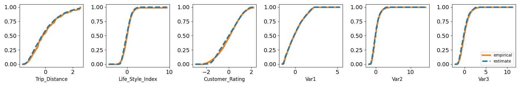
Figure 1: cabs dataset. Empirical (solid orange) and estimated (dashed blue) CDFs of continuous and ordinal variables (Monte Carlo approximated with 5000 samples). We standardize covariates and remove observations outside the 1% and 99% percentile range.

Privacy preservability. The privacy preservability performances of synthesizers, as measured by the DCR, are presented in Table 4. DistVAE performs best in preserving privacy, with the highest DCR values compared to other methods. Notably, as the value of $\beta$ increases in DistVAE, the DCR between the real training and synthetic datasets (R&S) also increases. This indicates that the risk of privacy leakage can be controlled by adjusting $\beta$, where higher values of $\beta$ correspond to a higher level of privacy protection. Moreover, DistVAE consistently achieves large DCR values for the synthetic dataset (S) across all $\beta$ values, indicating its ability to generate diverse synthetic samples. On the other hand, CTAB-GAN generates duplicated records in the synthetic dataset, resulting in relatively lower DCR scores for the synthetic dataset (S). For detailed DCR scores for all tabular datasets, please refer to Appendix A.10.

Table 4: Privacy preservability: Averaged distance to closest record (DCR) between real training and synthetic datasets (R&S), between the same real training datasets (R), and between the same synthetic datasets (S). Mean and standard deviation values are obtained from 10 repeated experiments. The DCR (R) score represents the baseline diversity of datasets. Higher is better.

Model	R&S	R	S
CTGAN	$0.426_{\pm 0.229}$	$0.237_{\pm 0.153}$	$0.356_{\pm 0.202}$
TVAE	$0.470_{\pm 0.181}$	$0.237_{\pm 0.153}$	$0.278_{\pm 0.195}$
CTAB-GAN	$0.508_{\pm 0.259}$	$0.237_{\pm 0.153}$	$0.039_{\pm 0.073}$
DistVAE($\beta=0.5$)	$0.444_{\pm 0.250}$	$0.237_{\pm 0.153}$	$0.463_{\pm 0.288}$
DistVAE($\beta=1$)	$0.463_{\pm 0.282}$	$0.237_{\pm 0.153}$	$0.479_{\pm 0.310}$
DistVAE($\beta=5$)	$\textbf{0.517}_{\pm 0.272}$	$0.237_{\pm 0.153}$	$\textbf{0.511}_{\pm 0.335}$

Table 5: Privacy preservability: Averaged membership inference attack performance. Mean and standard deviation values are obtained from 10 repeated experiments.

Model	Accuracy	AUC
TVAE	$0.495_{\pm 0.019}$	$0.495_{\pm 0.019}$
DistVAE($\beta=0.5$)	$0.500_{\pm 0.003}$	$0.500_{\pm 0.003}$

To evaluate the membership inference attack, we prepare one attack model per class. The attack testing records comprise an equal number of real training and test records, distinguished by the labels $in$ and $out$, respectively. Note that the test records are not employed in constructing the attack models. We employ gradient-boosting classifiers as the attack models, and for computational feasibility, we limit the number of attack models to one (i.e., $C=1$).

For the membership inference attack evaluation, we utilize accuracy and AUC (Area Under Curve) as the evaluation metrics. Since the target labels ($in/out$) are balanced, and the task is a binary classification problem, these metrics are appropriate. The results presented in Table 5 reveal that both DistVAE and TVAE achieve nearly identical accuracy and AUC scores of 0.5. This indicates that the attack models can not distinguish between members of the real training and test datasets. Consequently, the membership inference attack is unsuccessful for both models. Therefore, DistVAE effectively generates synthetic datasets while ensuring privacy against membership inference attacks. A comprehensive assessment of membership inference attack performances for all tabular datasets can be found in Appendix A.10.

Table 6: Privacy preservability: Averaged attribute disclosure performance with the $F_{1}$ score. Mean and standard deviation values are obtained from 10 repeated experiments. Lower is better.

	Number of neighbors ($k$)
Model	1	10	100
CTGAN	$0.262_{\pm 0.091}$	$0.282_{\pm 0.087}$	$0.275_{\pm 0.087}$
TVAE	$0.437_{\pm 0.162}$	$0.438_{\pm 0.160}$	$0.432_{\pm 0.162}$
CTAB-GAN	$\textbf{0.257}_{\pm 0.123}$	$0.258_{\pm 0.114}$	$0.261_{\pm 0.111}$
DistVAE($\beta=0.5$)	$0.328_{\pm 0.088}$	$0.328_{\pm 0.076}$	$0.310_{\pm 0.072}$
DistVAE($\beta=1$)	$0.307_{\pm 0.073}$	$0.313_{\pm 0.068}$	$0.297_{\pm 0.066}$
DistVAE($\beta=5$)	$0.265_{\pm 0.105}$	$\textbf{0.253}_{\pm 0.103}$	$\textbf{0.232}_{\pm 0.101}$

We present the attribute disclosure performance results in Table 6. For each value of $k$, we observe that as $\beta$ increases, the $F_{1}$ score of DistVAE decreases. Also, DistVAE achieves the smallest $F_{1}$ score when $k$ equals 10 and 100. Based on these results, we can conclude that DistVAE can generate synthetic datasets with a low risk of attribute disclosure, and the level of privacy preservation is controlled by $\beta$. Please refer to Appendix A.10 for a detailed evaluation of attribute disclosure performance for all tabular datasets.

Quantile estimation. To investigate the quantile estimation performance, we also evaluate DistVAE using the Vrate($\alpha$) metric [11]. The Vrate($\alpha$) is defined as $\frac{1}{|I_{test}|}\sum_{i\in I_{test}}I(x_{i}<\hat{Q}_{\alpha})$, where $\alpha\in(0,1)$, $I_{test}$ is the set of indices for the test dataset, $x_{i}$ is the $i$-th sample in the test dataset, and $\hat{Q}_{\alpha}$ is the empirical $\alpha$-quantile of the synthetic data. Since Vrate($\alpha$) indicates the proportion of compliance samples in the test dataset, the Vrate($\alpha$) score should be close to $\alpha$.

Table 7: Averaged Vrate($\alpha$) and $|\alpha-\mbox{Vrate}(\alpha)|$.

$\alpha$	0.1	0.3	0.5	0.7	0.9
Vrate($\alpha$)	0.204	0.373	0.533	0.725	0.908
$|\alpha-\mbox{Vrate}(\alpha)|$	0.104	0.083	0.04	0.032	0.008

The Vrate($\alpha$) evaluation results are presented in Table 7. Table 7 shows that the ratio of violated test samples ($|\alpha-\mbox{Vrate}(\alpha)|$) decreases as $\alpha$ increases, indicating a better performance for estimating larger quantiles. However, the ratio of violated test samples is relatively large for smaller $\alpha$ values, which may be due to extremely skewed continuous variables, such as capital-gain and capital-loss from adult dataset, that make the quantile estimation unstable.

5 Conclusion and Limitations

This paper introduces a novel distributional learning method of VAE, which aims to effectively capture the underlying distribution of the observed dataset using a nonparametric approach. Our proposed method involves directly estimating CDFs using the CRPS loss while maintaining the mathematical derivation of the lower bound.

In our study, we confirm that the proposed decoder enhances the performance of generative models for tabular data. However, this conclusion relies on the assumption of conditional independence among the observed variables given the latent variable. When the dimension of the latent variable is small, this assumption is prone to violation. Therefore, in cases where the size of the latent space is limited, the proposed nonparametric fitting of the decoder might not accurately represent the underlying distribution. Particularly in the image domain, where adjacent pixel values exhibit significant dependence, it remains uncertain whether our proposed model would lead to notable improvements in image data generation with a low-dimensional latent space.

Nevertheless, classical image datasets, such as CIFAR-10 [36], often exhibit pixel value distributions that deviate considerably from Gaussian, with the frequencies of edge values (0 and 255) dominating more than other pixel values [16, 53]. Other image datasets, as presented in [48], demonstrate multi-modality in pixel value distributions. These experimental findings suggest that leveraging the capacity of distributional learning could be advantageous in approximating the ground-truth distribution of image data when the latent variable effectively captures conditional independence among the image pixels. Consequently, we expect that compromising biases arising from violating conditional independence and marginally misspecified distributions may further enhance our results, and we leave it for future research.

On the other hand, we consider two approaches to enhance the performance of quantile estimation. Firstly, we plan to extend the parameterization of conditional quantile functions to a more flexible monotonic regression model. Secondly, we intend to incorporate the Uniform Pessimistic Risk (UPR) [26] into the VAE framework to handle lower quantile levels better. Furthermore, we are exploring the expansion of DistVAE into a time-series distributional forecasting model by adopting the conditional VAE framework [56]. This extension will enable the application of our method to time-series data, opening new avenues for distributional forecasting.

Appendix A Appendix

A.1 Derivation of ELBO

$$\log p({\bf x};\theta,\beta)$$

$$= \log\sum_{k=1}^{K}p(\alpha_{k})\int p({\bf x}|{\bf z},\alpha_{k};\theta,\beta)p({\bf z})d{\bf z}$$

$$= \log\sum_{k=1}^{K}p(\alpha_{k})\int p({\bf x}|{\bf z},\alpha_{k};\theta,\beta)\frac{p({\bf z})}{q({\bf z}|{\bf x};\phi)}q({\bf z}|{\bf x};\phi)d{\bf z}$$

$$\geq \sum_{k=1}^{K}p(\alpha_{k})\int q({\bf z}|{\bf x};\phi)\log\Big{(}p({\bf x}|{\bf z},\alpha_{k};\theta,\beta)\frac{p({\bf z})}{q({\bf z}|{\bf x};\phi)}\Big{)}d{\bf z}$$

$$= \frac{1}{K}\sum_{k=1}^{K}\mathbb{E}_{q({\bf z}|{\bf x};\phi)}[\log p({\bf x}|{\bf z},\alpha_{k};\theta,\beta)]-\mathcal{KL}(q({\bf z}|{\bf x};\phi)\|p({\bf z}))$$

$$= \frac{1}{K}\sum_{k=1}^{K}\mathbb{E}_{q({\bf z}|{\bf x};\phi)}\left[\sum_{j\in I_{C}}\log p({\bf x}_{j}|{\bf z},\alpha_{k};\theta_{j},\beta)+\sum_{j\in I_{D}}\log p({\bf x}_{j}|{\bf z};\theta_{j},\beta)\right]-\mathcal{KL}(q({\bf z}|{\bf x};\phi)\|p({\bf z}))$$

$$= \mathbb{E}_{q({\bf z}|{\bf x};\phi)}\left[\sum_{j\in I_{C}}\frac{1}{K}\sum_{k=1}^{K}\log\frac{\alpha_{k}(1-\alpha_{k})}{\beta}-\rho_{\alpha_{k}}\left(\frac{{\bf x}_{j}-D_{j}(\alpha_{k}|{\bf z},\theta_{j})}{\beta}\right)\right]$$

$$+\mathbb{E}_{q({\bf z}|{\bf x};\phi)}\left[\sum_{j\in I_{D}}\sum_{l=1}^{T_{j}}I({\bf x}_{j}=l)\cdot\log\pi_{l}({\bf z};\theta_{j})\right]-\mathcal{KL}(q({\bf z}|{\bf x};\phi)\|p({\bf z}))$$

$$= \mathbb{E}_{q({\bf z}|{\bf x};\phi)}\left[-\frac{1}{\beta}\cdot\sum_{j\in I_{C}}\frac{1}{K}\sum_{k=1}^{K}\rho_{\alpha_{k}}\Big{(}{\bf x}_{j}-D_{j}(\alpha_{k}|{\bf z},\theta_{j})\Big{)}\right]+\frac{p}{K}\sum_{k=1}^{K}\log\alpha_{k}(1-\alpha_{k})-p\cdot\log\beta$$

$$+\mathbb{E}_{q({\bf z}|{\bf x};\phi)}\left[\sum_{j\in I_{D}}\sum_{l=1}^{T_{j}}I({\bf x}_{j}=l)\cdot\log\pi_{l}({\bf z};\theta_{j})\right]-\mathcal{KL}(q({\bf z}|{\bf x};\phi)\|p({\bf z}))$$

$$= -\frac{1}{\beta}\Bigg{(}\mathbb{E}_{q({\bf z}|{\bf x};\phi)}\left[\sum_{j\in I_{C}}\frac{1}{K}\sum_{k=1}^{K}\rho_{\alpha_{k}}\Big{(}{\bf x}_{j}-D_{j}(\alpha_{k}|{\bf z},\theta_{j})\Big{)}\right]-\beta\frac{p}{K}\sum_{k=1}^{K}\log\alpha_{k}(1-\alpha_{k})+\beta p\cdot\log\beta$$

$$-\beta\cdot\mathbb{E}_{q({\bf z}|{\bf x};\phi)}\left[\sum_{j\in I_{D}}\sum_{l=1}^{T_{j}}I({\bf x}_{j}=l)\cdot\log\pi_{l}({\bf z};\theta_{j})\right]+\beta\cdot\mathcal{KL}(q({\bf z}|{\bf x};\phi)\|p({\bf z}))\Bigg{)},$$

by Jensen’s inequality.

A.2 Proof of Theorem 1

Proof.

$$\mathbb{E}_{p({\bf x})}\mathbb{E}_{q({\bf z}|{\bf x};\phi)}\left[\frac{1}{K}\sum_{k=1}^{K}\rho_{\alpha_{k}}\Big{(}{\bf x}_{j}-D_{j}(\alpha_{k}|{\bf z},\theta_{j})\Big{)}\right] = \frac{1}{K}\sum_{k=1}^{K}h(\alpha_{k})$$

$$= \sum_{k=1}^{K}h(\alpha_{k})\cdot(\alpha_{k}-\alpha_{k-1}),$$

where $\alpha_{0}\coloneqq 0$ and $\mathbb{E}_{p({\bf x})}\mathbb{E}_{q({\bf z}|{\bf x};\phi)}\left[\rho_{\alpha_{k}}\Big{(}{\bf x}_{j}-D_{j}(\alpha_{k}|{\bf z},\theta_{j})\Big{)}\right]$ is denoted as $h(\alpha_{k})$.

Since $\alpha_{k}\in[\alpha_{k-1},\alpha_{k}]$ and $h(\cdot):[0,1]\mapsto\mathbb{R}$ is a continuous function, for $j\in I_{C}$,

$$\lim_{K\rightarrow\infty}\mathbb{E}_{p({\bf x})}\mathbb{E}_{q({\bf z}|{\bf x};\phi)}\left[\frac{1}{K}\sum_{k=1}^{K}\rho_{\alpha_{k}}\Big{(}{\bf x}_{j}-D_{j}(\alpha_{k}|{\bf z},\theta_{j})\Big{)}\right] = \lim_{K\rightarrow\infty}\sum_{k=1}^{K}h(\alpha_{k})\cdot(\alpha_{k}-\alpha_{k-1})$$

$$= \int_{0}^{1}h(\alpha)d\alpha$$

$$= \int_{0}^{1}\mathbb{E}_{p({\bf x})}\mathbb{E}_{q({\bf z}|{\bf x};\phi)}\left[\rho_{\alpha}\Big{(}{\bf x}_{j}-D_{j}(\alpha|{\bf z},\theta_{j})\Big{)}\right]d\alpha$$

$$= \mathbb{E}_{p({\bf x})}\mathbb{E}_{q({\bf z}|{\bf x};\phi)}\left[\int_{0}^{1}\rho_{\alpha}\Big{(}{\bf x}_{j}-D_{j}(\alpha|{\bf z},\theta_{j})\Big{)}d\alpha\right],$$

by the definition of the Riemann integral and the Fubini-Tonelli theorem. The proof is complete. ∎

A.3 Proof of Theorem 2

Proof.

$$\min_{\theta}\mathbb{E}_{p({\bf x})q({\bf z}|{\bf x};\phi)}\sum_{j=1}^{p}\int_{0}^{1}\rho_{\alpha}({\bf x}_{j}-D_{j}(\alpha,{\bf z};\theta_{j}))d\alpha = \mathbb{E}_{q({\bf z};\phi)q({\bf x}|{\bf z};\phi)}\sum_{j=1}^{p}\int_{0}^{1}\rho_{\alpha}({\bf x}_{j}-D_{j}(\alpha,{\bf z};\theta_{j}))d\alpha$$

$$= \sum_{j=1}^{p}\mathbb{E}_{q({\bf z};\phi)}\mathbb{E}_{q({\bf x}_{j}|{\bf z};\phi)}\int_{0}^{1}\rho_{\alpha}({\bf x}_{j}-D_{j}(\alpha,{\bf z};\theta_{j}))d\alpha.$$

So, for all $j=1,\cdots,p$,

$$\theta_{j}^{*}(\phi)\in\arg\min_{\theta_{j}}\mathbb{E}_{q({\bf z};\phi)}\mathbb{E}_{q({\bf x}_{j}|{\bf z};\phi)}\int_{0}^{1}\rho_{\alpha}({\bf x}_{j}-D_{j}(\alpha,{\bf z};\theta_{j}))d\alpha,$$

and it is proper scoring rule relative to $F_{j}(\cdot|{\bf z};\phi)$ for all ${\bf z}\in\mathbb{R}^{d}$. It implies that $D_{j}^{-1}({\bf x}_{j},{\bf z};\theta_{j}^{*}(\phi))=F_{j}({\bf x}_{j}|{\bf z};\phi)$, and $\frac{d}{d{\bf x}_{j}}D_{j}^{-1}({\bf x}_{j},{\bf z};\theta_{j}^{*}(\phi))=q_{j}({\bf x}_{j}|{\bf z};\phi)$, for all ${\bf x}_{j}\in\mathbb{R}$, by Assumption 2.

It follows that

$$\int\prod_{j=1}^{p}\frac{d}{d{\bf x}_{j}}D_{j}^{-1}({\bf x}_{j},{\bf z};\theta_{j}^{*}(\phi))q({\bf z};\phi)d{\bf z} = \int\prod_{j=1}^{p}q_{j}({\bf x}_{j}|{\bf z};\phi)q({\bf z};\phi)d{\bf z}$$

$$= \int q({\bf x}|{\bf z};\phi)q({\bf z};\phi)d{\bf z}$$

$$= \int\frac{p({\bf x})q({\bf z}|{\bf x};\phi)}{q({\bf z};\phi)}q({\bf z};\phi)d{\bf z}$$

$$= \int p({\bf x})q({\bf z}|{\bf x};\phi)d{\bf z}$$

$$= p({\bf x}).$$

The proof is complete. ∎

A.4 Proof of Theorem 3

Proof.

$$\min_{\theta}\mathbb{E}_{p({\bf x})q({\bf z}|{\bf x};\phi)}\sum_{j=1}^{p}\int_{0}^{1}\rho_{\alpha}({\bf x}_{j}-D_{j}(\alpha,{\bf z};\theta_{j}))d\alpha = \mathbb{E}_{q({\bf z};\phi)q({\bf x}|{\bf z};\phi)}\sum_{j=1}^{p}\int_{0}^{1}\rho_{\alpha}({\bf x}_{j}-D_{j}(\alpha,{\bf z};\theta_{j}))d\alpha$$

$$= \sum_{j=1}^{p}\mathbb{E}_{q({\bf z};\phi)}\mathbb{E}_{q({\bf x}_{j}|{\bf z};\phi)}\int_{0}^{1}\rho_{\alpha}({\bf x}_{j}-D_{j}(\alpha,{\bf z};\theta_{j}))d\alpha.$$

So, for all $j=1,\cdots,p$,

$$\theta_{j}^{*}(\phi)\in\arg\min_{\theta_{j}}\mathbb{E}_{q({\bf z};\phi)}\mathbb{E}_{q({\bf x}_{j}|{\bf z};\phi)}\int_{0}^{1}\rho_{\alpha}({\bf x}_{j}-D_{j}(\alpha,{\bf z};\theta_{j}))d\alpha,$$

and it is proper scoring rule relative to $F_{j}(\cdot|{\bf z};\phi)$ for all ${\bf z}\in\mathbb{R}^{d}$. It implies that $D_{j}^{-1}({\bf x}_{j},{\bf z};\theta_{j}^{*}(\phi))=F_{j}({\bf x}_{j}|{\bf z};\phi)$, and $\frac{d}{d{\bf x}_{j}}D_{j}^{-1}({\bf x}_{j},{\bf z};\theta_{j}^{*}(\phi))=q_{j}({\bf x}_{j}|{\bf z};\phi)$, for all ${\bf x}_{j}\in\mathbb{R}$, by Assumption 2.

It follows that

$$\mathcal{KL}\left(p({\bf x})\Bigg{\|}\int\prod_{j=1}^{p}\frac{d}{d{\bf x}_{j}}D_{j}^{-1}({\bf x}_{j},{\bf z};\theta_{j}^{*}(\phi))p({\bf z})d{\bf z}\right) = \mathcal{KL}\left(p({\bf x})\Bigg{\|}\int\prod_{j=1}^{p}q_{j}({\bf x}_{j}|{\bf z};\phi)p({\bf z})d{\bf z}\right)$$

$$= \mathcal{KL}\left(p({\bf x})\Bigg{\|}\int q({\bf x}|{\bf z};\phi)p({\bf z})d{\bf z}\right)$$

$$= \mathcal{KL}\left(p({\bf x})\Bigg{\|}\int\frac{p({\bf x})q({\bf z}|{\bf x};\phi)}{q({\bf z};\phi)}p({\bf z})d{\bf z}\right)$$

$$= \mathcal{KL}\left(p({\bf x})\Bigg{\|}p({\bf x})\int\frac{p({\bf z})q({\bf z}|{\bf x};\phi)}{q({\bf z};\phi)}d{\bf z}\right)$$

$$= \mathbb{E}_{p({\bf x})}\left[-\log\int\frac{p({\bf z})q({\bf z}|{\bf x};\phi)}{q({\bf z};\phi)}d{\bf z}\right]$$

$$\leq \mathbb{E}_{p({\bf x})}\left[\int q({\bf z}|{\bf x};\phi)\log\frac{q({\bf z};\phi)}{p({\bf z})}d{\bf z}\right]$$

$$= \iint p({\bf x})q({\bf z}|{\bf x};\phi)\log\frac{q({\bf z};\phi)}{p({\bf z})}d{\bf z}d{\bf x}$$

$$= \iint p({\bf x})q({\bf z}|{\bf x};\phi)\log\frac{q({\bf z};\phi)}{p({\bf z})}d{\bf x}d{\bf z}$$

$$= \int q({\bf z};\phi)\log\frac{q({\bf z};\phi)}{p({\bf z})}d{\bf z}$$

$$= \mathcal{KL}(q({\bf z};\phi)\|p({\bf z}))$$

$$< \epsilon,$$

by Jensen’s inequality, Fubini-Tonelli theorem, and the assumptions. The proof is complete. ∎

A.5 Closed Form Loss

$$2\cdot\int_{0}^{1}\rho_{\alpha}\Big{(}{\bf x}_{j}-D_{j}(\alpha,{\bf z},\theta_{j})\Big{)}d\alpha = (2\tilde{\alpha}_{j}-1){\bf x}_{j}+(1-2\tilde{\alpha}_{j})\gamma^{(j)}({\bf z})$$

$$+ \sum_{m=1}^{M}b_{m}^{(j)}({\bf z})\Bigg{(}\frac{1-d_{m}^{3}}{3}-d_{m}-\max(\tilde{\alpha}_{j},d_{m})^{2}+2\max(\tilde{\alpha}_{j},d_{m})d_{m}\Bigg{)},$$

where $D_{j}(\tilde{\alpha}_{j},{\bf z};\theta_{j})={\bf x}_{j}$, $\tilde{\alpha}_{j}=\frac{{\bf x}_{j}-\gamma^{(j)}({\bf z})+\sum_{m=0}^{m_{0}}b_{m}^{(j)}({\bf z})d_{m}}{\sum_{m=0}^{m_{0}}b_{m}^{(j)}({\bf z})}$, and $D_{j}(d_{m_{0}},{\bf z};\theta_{j})\leq{\bf x}_{j}\leq D_{j}(d_{m_{0}+1},{\bf z};\theta_{j})$.

A.6 Discretization of Estimated CDF

To ensure appropriate discretization of the estimated CDF for ordinal variables, we propose a post-ad-hoc discretization step [53]. We focus on the case where $p=1$ and $q=0$ for brevity. We denote the set of observed possible values for the ordinal variable as ${x^{(1)},x^{(2)},\cdots,x^{(m)}}$. The discretization algorithm for the estimated CDF is presented in Algorithm 1, and we provide an example of the discretization algorithm’s outcome in Figure 2.

Algorithm 1 Discretization of Estimated CDF

Input $\{x^{(1)},x^{(2)},\cdots,x^{(m)}\}$, Estimated CDF $\hat{F}(\cdot;\theta)$

Output Discretized CDF $\hat{F}^{*}(\cdot;\theta)$

(1) Compute $\hat{F}(x^{(i)}-0.5;\theta)$ and $\hat{F}(x^{(i)}+0.5;\theta)$ for $i=1,\cdots,m$.

(2) Discretization: For $i=1,\cdots,m$,

$$\hat{F}^{*}(x^{(i)};\theta) \coloneqq \hat{F}^{*}(x^{(i-1)};\theta)$$

$$+ \hat{F}(x^{(i)}+0.5;\theta)-\hat{F}(x^{(i)}-0.5;\theta),$$

where $\hat{F}^{*}(x^{(0)};\theta)\coloneqq 0$.

(3) Ensure monotonicity: For $i=1,\cdots,m-1$, if $\hat{F}^{*}(x^{(i)};\theta)>\hat{F}^{*}(x^{(i+1)};\theta)$,

$$\hat{F}^{*}(x^{(i+1)};\theta)\coloneqq\hat{F}^{*}(x^{(i)};\theta).$$

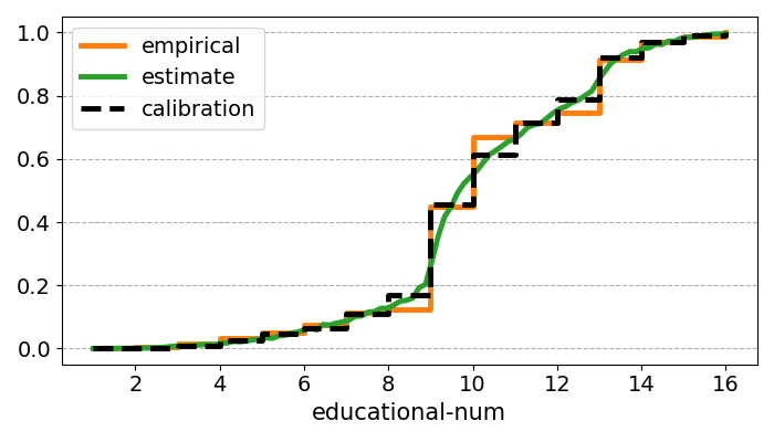
Figure 2: Discretized CDF for ordinal variable educational-num of adult dataset. ‘estimate’ indicates $\hat{F}(\cdot;\theta)$, ‘calibration’ indicates $\hat{F}^{*}(\cdot;\theta)$, and ‘empirical’ indicates the empirical CDF of the observed dataset.

A.7 Membership Inference Attack

[47] propose the customized membership inference attack method of [54] to attack the GAN-based synthesizer. Similarly, we propose the customized membership inference attack method of [54] to attack the VAE-based synthesizer.

Assumption 3 ([54]).

In the membership inference attack, the attacker attacks the target model under the following assumptions:

• The attacker is only allowed for black-box access, where the attacker can only supply inputs to the model and receive the model’s output(s).

• The attacker can obtain as many outputs as they want from a target model to attack.

• The real and synthetic datasets should not have common records.

• The attacker knows the algorithm and architecture of the target model.

Denote $D_{train}^{*}$ and $D_{test}^{*}$ as the real training and test datasets. Under Assumption 3, the overall steps of the membership inference attack are outlined below:

1. Generate shadow training and test datasets $D_{train}^{(i)},D_{test}^{(i)},i=1,\cdots,C$ from $M^{*}$ by (A1), where $M^{*}$ is the model attacker wants to attack. By (A2), the attacker is allowed to obtain shadow datasets such as $|D_{train}^{(i)}|=|D_{train}^{*}|$ and $D_{train}^{(i)}\cap D_{test}^{(j)}=\varnothing$, for $i=1,\cdots,C$. Under (A3), $D_{train}^{(i)}\cap D_{train}^{*}=\varnothing$, for $i=1,\cdots,C$.

2. Train shadow models $M_{1},\cdots,M_{C}$ under (A4), i.e., each shadow model is trained similarly to the target model $M^{*}$.

3. For $i=1,\cdots,C$,

   1. Obtain representation vectors ${\bf z}$ from the encoder of $M_{i}$ with the input of $D_{train}^{(i)}$. Then, attacking training records are $({\bf y},{\bf z},in)$.

   2. Obtain representation vectors ${\bf z}$ from the encoder of $M_{i}$ with the input of $D_{test}^{(i)}$. Then, attacking training records are $({\bf y},{\bf z},out)$.

   where ${\bf y}$ is the labels of shadow dataset records. And we assume that ${\bf y}$ consists of the MLu classification target.

4. Merge all attack training records, $({\bf y},{\bf z},in/out)$.

5. For each class of ${\bf y}$, train attack model which is a binary classification model which classifies $in/out$ based on the representation vectors ${\bf z}$.

6. Now it is ready to attack.

Note that we use the representation vector of VAE instead of the output of the GAN discriminator [47].

A.8 Dataset Descriptions

Websites

• covertype: https://www.kaggle.com/datasets/uciml/forest-cover-type-dataset

• credit: https://www.kaggle.com/c/home-credit-default-risk

• loan: https://www.kaggle.com/datasets/teertha/personal-loan-modeling

• adult: https://www.kaggle.com/datasets/uciml/adult-census-income

• cabs: https://www.kaggle.com/datasets/arashnic/taxi-pricing-with-mobility-analytics?select=test.csv

• kings: https://www.kaggle.com/datasets/harlfoxem/housesalesprediction

Table 8: Description of datasets. #C represents the number of continuous and ordinal variables. #D denotes the number of discrete variables.

Dataset	Train/Test Split	Regression Target	Classification Target	#C	#D
covertype	45k/5k	Elevation	Cover_Type	10	1
credit	45k/5k	AMT_CREDIT	TARGET	10	9
loan	4k/1k	Age	Personal Loan	5	6
adult	40k/5k	age	income	5	9
cabs	40k/1k	Trip_Distance	Surge_Pricing_Type	6	7
kings	20k/1k	long	condition	11	7

A.9 Experimental Settings

We run all experiments using Geforce RTX 3090 GPU, and our experimental codes are all available with pytorch.

Table 9: Hyper-parameter settings for tabular dataset experiments.

Model	epochs	batch size	learning rate	$\beta$ (or decoder std range)	$d$	$M$
CTGAN	300	500	0.0002	-	2	-
TVAE	200	256	0.005	[0.1, 1]	2	-
CTAB-GAN	150	500	0.0002	-	2	-
DistVAE	100	256	0.001	0.5	2	10

Table 10: The number of model parameters for tabular dataset experiments.

Model	covtype	credit	adult	loan	cabs	kings
CTGAN	20k	32k	52k	13k	30k	51k
TVAE	10k	12k	13k	6k	10k	10k
CTAB-GAN	12k	13k	14k	5k	12k	15k
DistVAE	10k	12k	13k	6k	10k	16k

Table 11: Classifier and regressor used to evaluate synthetic data quality. The names of all parameters used in the description are consistent with those defined in corresponding packages.

Tasks	Model	Description
Regression	Linear Regression	Package: statsmodels.api.sm.OLS, setting: without intercept, defaulted values
	Random Forest	Package: sklearn.ensemble.RandomForestRegressor, setting: random_state=0, defaulted values
	Gradient Boosting	Package: sklearn.ensemble.GradientBoostingRegressor, setting: random_state=0, defaulted values
Classification	Logistic Regression	Package: sklearn.linear_model.LogisticRegression, setting: multi_class=’ovr’, fit_intercept=False, defaulted values
	Random Forest	Package: sklearn.ensemble.RandomForestClassifier, setting: random_state=0, defaulted values
	Gradient Boosting	Package: sklearn.ensemble.GradientBoostingClassifier, setting: random_state=0, defaulted values

A.10 Detailed Experimental Results

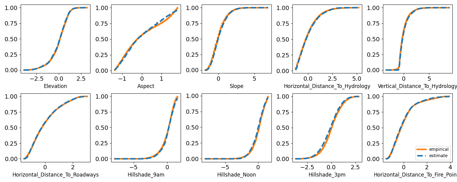
(a) covtype

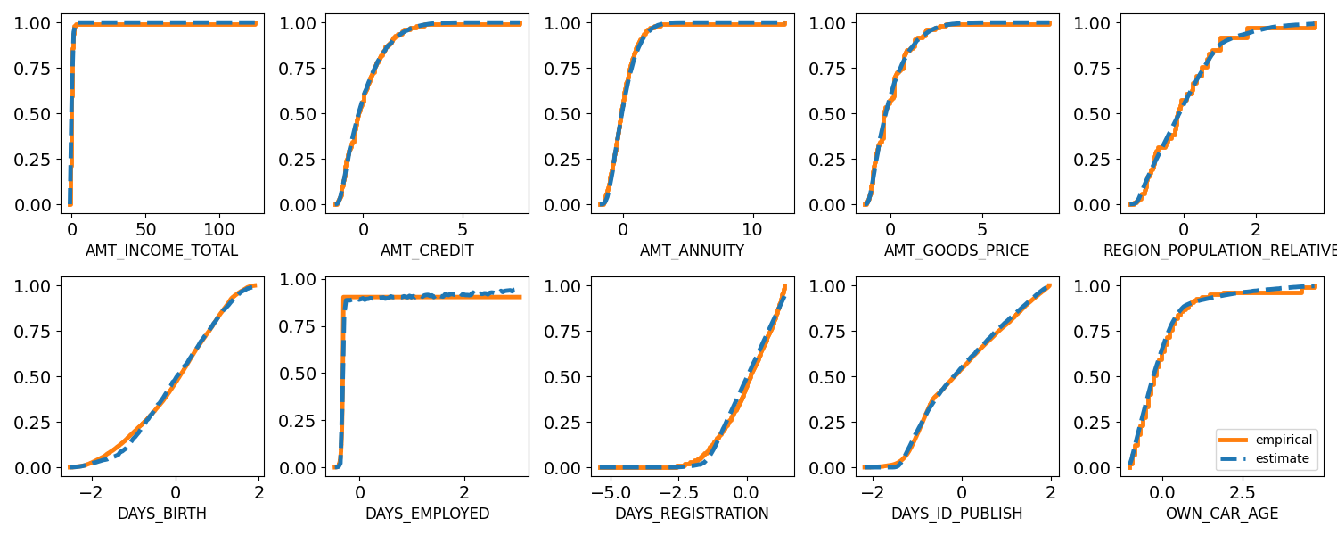
(b) credit

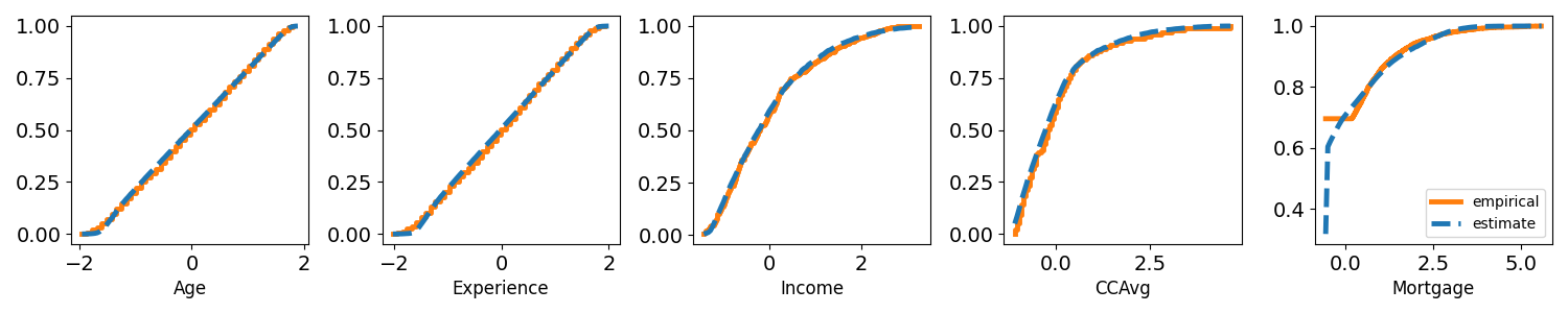
(c) loan

Figure 3: Empirical and estimated CDFs of continuous and count variables (Monte Carlo approximated with 5000 samples). We standardize covariates and remove observations outside the 1% and 99% percentile range.

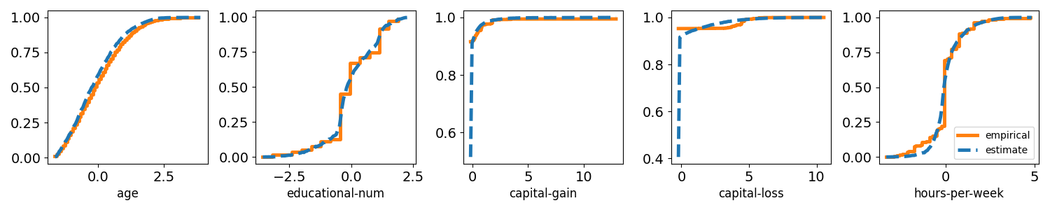
(a) adult

(b) cabs

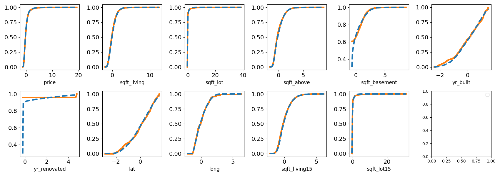
(c) kings

Figure 4: Empirical and estimated CDFs of continuous and count variables (Monte Carlo approximated with 5000 samples). We standardize covariates and remove observations outside the 1% and 99% percentile range.

Table 12: MLu metrics (MARE, $F_{1}$). Mean and standard deviation values are obtained from 10 repeated experiments. $\uparrow$ denotes higher is better and $\downarrow$ denotes lower is better.

Dataset	covertype		credit		loan
Model	MARE $\downarrow$	$F_{1}$ $\uparrow$	MARE $\downarrow$	$F_{1}$ $\uparrow$	MARE $\downarrow$	$F_{1}$ $\uparrow$
Baseline	0.035	0.718	0.064	0.927	0.020	0.948
CTGAN	$0.058_{\pm 0.007}$	$0.227_{\pm 0.030}$	$0.593_{\pm 0.150}$	$0.914_{\pm 0.006}$	$0.258_{\pm 0.020}$	$0.842_{\pm 0.109}$
TVAE	$0.079_{\pm 0.007}$	$0.504_{\pm 0.032}$	$0.260_{\pm 0.135}$	$0.091_{\pm 0.286}$	$0.124_{\pm 0.033}$	$0.785_{\pm 0.288}$
CTAB-GAN	$0.065_{\pm 0.004}$	$0.493_{\pm 0.027}$	$0.887_{\pm 0.351}$	$0.913_{\pm 0.005}$	$0.247_{\pm 0.019}$	$0.887_{\pm 0.026}$
DistVAE($\beta=0.5$)	$0.044_{\pm 0.002}$	$0.605_{\pm 0.006}$	$0.763_{\pm 0.068}$	$0.926_{\pm 0.001}$	$0.249_{\pm 0.007}$	$0.914_{\pm 0.009}$
DistVAE($\beta=1$)	$0.045_{\pm 0.001}$	$0.557_{\pm 0.007}$	$0.774_{\pm 0.035}$	$0.926_{\pm 0.000}$	$0.249_{\pm 0.005}$	$0.897_{\pm 0.002}$
DistVAE($\beta=5$)	$0.063_{\pm 0.001}$	$0.443_{\pm 0.018}$	$0.870_{\pm 0.022}$	$0.904_{\pm 0.010}$	$0.249_{\pm 0.005}$	$0.893_{\pm 0.005}$

Dataset	adult		cabs		kings
Model	MARE $\downarrow$	$F_{1}$ $\uparrow$	MARE $\downarrow$	$F_{1}$ $\uparrow$	MARE $\downarrow$	$F_{1}$ $\uparrow$
Baseline	0.216	0.854	0.565	0.743	0.001	0.695
CTGAN	$0.297_{\pm 0.030}$	$0.796_{\pm 0.022}$	$0.721_{\pm 0.046}$	$0.674_{\pm 0.024}$	$0.001_{\pm 0.000}$	$0.579_{\pm 0.035}$
TVAE	$0.238_{\pm 0.006}$	$0.809_{\pm 0.016}$	$0.642_{\pm 0.035}$	$0.689_{\pm 0.031}$	$0.010_{\pm 0.005}$	$0.687_{\pm 0.041}$
CTAB-GAN	$0.321_{\pm 0.036}$	$0.730_{\pm 0.069}$	$0.894_{\pm 0.116}$	$0.582_{\pm 0.047}$	$0.001_{\pm 0.000}$	$0.608_{\pm 0.022}$
DistVAE($\beta=0.5$)	$0.232_{\pm 0.004}$	$0.825_{\pm 0.009}$	$0.803_{\pm 0.129}$	$0.707_{\pm 0.010}$	$0.001_{\pm 0.000}$	$0.640_{\pm 0.002}$
DistVAE($\beta=1$)	$0.234_{\pm 0.006}$	$0.822_{\pm 0.003}$	$0.760_{\pm 0.062}$	$0.725_{\pm 0.004}$	$0.001_{\pm 0.000}$	$0.644_{\pm 0.003}$
DistVAE($\beta=5$)	$0.327_{\pm 0.008}$	$0.751_{\pm 0.010}$	$0.839_{\pm 0.042}$	$0.447_{\pm 0.009}$	$0.002_{\pm 0.000}$	$0.637_{\pm 0.004}$

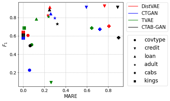
Figure 5: Machine learning utilities for compared models and real tabular datasets.

For a detailed comparison of the models and their performance, we present the paired (MARE, $F_{1}$) scores for all tabular datasets in Figure 5. A better score, indicating a superior performance in terms of MLu, is represented by a dot located in the upper left corner. Notably, Figure 5 consistently demonstrates that DistVAE achieves the best or at least competitive MLu across all tabular datasets. TVAE exhibits a notably low $F_{1}$ score in the credit dataset because it fails to handle the highly imbalanced discrete target variable. This comparative analysis highlights the strong MLu performance of DistVAE and the specific limitations of TVAE in certain scenarios.

Table 13: Correlation structure similarity. ‘CorrDist’ represents $L_{2}$ distance between the correlation matrix of synthetic and real datasets. Mean and standard deviation values are obtained from 10 repeated experiments. Lower is better.

Dataset	covertype	credit	loan	adult	cabs	kings
Model	CorrDist	CorrDist	CorrDist	CorrDist	CorrDist	CorrDist
CTGAN	$2.167_{\pm 0.419}$	$2.323_{\pm 0.362}$	$2.282_{\pm 0.177}$	$1.788_{\pm 0.217}$	$1.679_{\pm 0.129}$	$2.839_{\pm 0.246}$
TVAE	$1.969_{\pm 0.146}$	$4.021_{\pm 0.451}$	$2.404_{\pm 0.408}$	$2.231_{\pm 0.269}$	$3.136_{\pm 0.686}$	$2.665_{\pm 0.296}$
CTAB-GAN	$2.351_{\pm 0.185}$	$2.696_{\pm 0.275}$	$2.073_{\pm 0.110}$	$2.387_{\pm 0.470}$	$2.532_{\pm 0.225}$	$3.411_{\pm 0.399}$
DistVAE($\beta=0.5$)	$1.179_{\pm 0.090}$	$2.072_{\pm 0.162}$	$1.654_{\pm 0.050}$	$0.830_{\pm 0.078}$	$1.481_{\pm 0.071}$	$1.559_{\pm 0.135}$
DistVAE($\beta=1$)	$2.359_{\pm 0.018}$	$2.229_{\pm 0.102}$	$1.910_{\pm 0.019}$	$0.746_{\pm 0.042}$	$1.495_{\pm 0.047}$	$1.621_{\pm 0.149}$
DistVAE($\beta=5$)	$2.946_{\pm 0.007}$	$3.161_{\pm 0.006}$	$2.113_{\pm 0.015}$	$3.186_{\pm 0.007}$	$1.930_{\pm 0.004}$	$5.339_{\pm 0.006}$

Table 14: Marginal statistical similarity. K-S denotes the Kolmogorov–Smirnov statistic and 1-WD represents the 1-Wasserstein distance. Mean and standard deviation values are obtained from 10 repeated experiments. Lower is better.

Dataset	covertype		credit		loan
Model	K-S	1-WD	K-S	1-WD	K-S	1-WD
CTGAN	$0.080_{\pm 0.011}$	$0.108_{\pm 0.014}$	$0.132_{\pm 0.017}$	$0.088_{\pm 0.013}$	$0.112_{\pm 0.055}$	$0.061_{\pm 0.016}$
TVAE	$0.088_{\pm 0.008}$	$0.156_{\pm 0.018}$	$0.156_{\pm 0.036}$	$0.200_{\pm 0.035}$	$0.162_{\pm 0.024}$	$0.201_{\pm 0.024}$
CTAB-GAN	$0.073_{\pm 0.011}$	$0.096_{\pm 0.014}$	$0.140_{\pm 0.021}$	$0.111_{\pm 0.013}$	$0.181_{\pm 0.070}$	$0.153_{\pm 0.023}$
DistVAE($\beta=0.5$)	$0.032_{\pm 0.003}$	$0.041_{\pm 0.005}$	$0.088_{\pm 0.014}$	$0.089_{\pm 0.004}$	$0.060_{\pm 0.010}$	$0.048_{\pm 0.003}$
DistVAE($\beta=1$)	$0.049_{\pm 0.001}$	$0.079_{\pm 0.001}$	$0.084_{\pm 0.008}$	$0.093_{\pm 0.002}$	$0.056_{\pm 0.003}$	$0.054_{\pm 0.002}$
DistVAE($\beta=5$)	$0.064_{\pm 0.001}$	$0.112_{\pm 0.000}$	$0.146_{\pm 0.003}$	$0.113_{\pm 0.001}$	$0.057_{\pm 0.003}$	$0.056_{\pm 0.002}$

(a) Continuous

Dataset	adult		cabs		kings
Model	K-S	1-WD	K-S	1-WD	K-S	1-WD
CTGAN	$0.323_{\pm 0.126}$	$0.086_{\pm 0.017}$	$0.045_{\pm 0.007}$	$0.060_{\pm 0.011}$	$0.109_{\pm 0.012}$	$0.116_{\pm 0.016}$
TVAE	$0.477_{\pm 0.053}$	$0.414_{\pm 0.070}$	$0.098_{\pm 0.008}$	$0.139_{\pm 0.023}$	$0.195_{\pm 0.018}$	$0.213_{\pm 0.046}$
CTAB-GAN	$0.275_{\pm 0.122}$	$0.178_{\pm 0.053}$	$0.086_{\pm 0.008}$	$0.118_{\pm 0.015}$	$0.188_{\pm 0.035}$	$0.128_{\pm 0.019}$
DistVAE($\beta=0.5$)	$0.209_{\pm 0.064}$	$0.114_{\pm 0.009}$	$0.044_{\pm 0.003}$	$0.067_{\pm 0.003}$	$0.110_{\pm 0.008}$	$0.089_{\pm 0.003}$
DistVAE($\beta=1$)	$0.138_{\pm 0.041}$	$0.111_{\pm 0.007}$	$0.046_{\pm 0.002}$	$0.068_{\pm 0.003}$	$0.115_{\pm 0.007}$	$0.093_{\pm 0.002}$
DistVAE($\beta=5$)	$0.115_{\pm 0.005}$	$0.234_{\pm 0.002}$	$0.052_{\pm 0.001}$	$0.074_{\pm 0.002}$	$0.120_{\pm 0.002}$	$0.137_{\pm 0.002}$

(b) Continuous

Dataset	covertype		credit		loan
Model	K-S	1-WD	K-S	1-WD	K-S	1-WD
CTGAN	$0.591_{\pm 0.003}$	$1.629_{\pm 0.011}$	$0.061_{\pm 0.008}$	$0.147_{\pm 0.024}$	$0.070_{\pm 0.010}$	$0.076_{\pm 0.013}$
TVAE	$0.238_{\pm 0.042}$	$0.606_{\pm 0.033}$	$0.583_{\pm 0.045}$	$1.566_{\pm 0.116}$	$0.193_{\pm 0.028}$	$0.221_{\pm 0.043}$
CTAB-GAN	$0.052_{\pm 0.028}$	$0.180_{\pm 0.126}$	$0.034_{\pm 0.006}$	$0.076_{\pm 0.018}$	$0.039_{\pm 0.011}$	$0.046_{\pm 0.013}$
DistVAE($\beta=0.5$)	$0.023_{\pm 0.010}$	$0.073_{\pm 0.046}$	$0.020_{\pm 0.003}$	$0.046_{\pm 0.006}$	$0.019_{\pm 0.005}$	$0.027_{\pm 0.008}$
DistVAE($\beta=1$)	$0.011_{\pm 0.005}$	$0.036_{\pm 0.025}$	$0.018_{\pm 0.001}$	$0.042_{\pm 0.003}$	$0.011_{\pm 0.002}$	$0.015_{\pm 0.005}$
DistVAE($\beta=5$)	$0.109_{\pm 0.003}$	$0.379_{\pm 0.014}$	$0.027_{\pm 0.001}$	$0.068_{\pm 0.004}$	$0.009_{\pm 0.002}$	$0.013_{\pm 0.005}$

(c) Discrete

Dataset	adult		cabs		kings
Model	K-S	1-WD	K-S	1-WD	K-S	1-WD
CTGAN	$0.065_{\pm 0.008}$	$0.463_{\pm 0.051}$	$0.069_{\pm 0.016}$	$0.238_{\pm 0.036}$	$0.140_{\pm 0.018}$	$0.529_{\pm 0.064}$
TVAE	$0.479_{\pm 0.048}$	$5.228_{\pm 0.273}$	$0.411_{\pm 0.088}$	$1.202_{\pm 0.212}$	$0.405_{\pm 0.034}$	$1.262_{\pm 0.099}$
CTAB-GAN	$0.169_{\pm 0.018}$	$0.745_{\pm 0.294}$	$0.086_{\pm 0.013}$	$0.443_{\pm 0.074}$	$0.255_{\pm 0.027}$	$0.979_{\pm 0.107}$
DistVAE($\beta=0.5$)	$0.037_{\pm 0.004}$	$0.248_{\pm 0.026}$	$0.060_{\pm 0.017}$	$0.241_{\pm 0.084}$	$0.022_{\pm 0.004}$	$0.071_{\pm 0.012}$
DistVAE($\beta=1$)	$0.031_{\pm 0.004}$	$0.239_{\pm 0.019}$	$0.070_{\pm 0.003}$	$0.292_{\pm 0.010}$	$0.023_{\pm 0.003}$	$0.073_{\pm 0.008}$
DistVAE($\beta=5$)	$0.070_{\pm 0.002}$	$0.457_{\pm 0.010}$	$0.083_{\pm 0.003}$	$0.326_{\pm 0.011}$	$0.059_{\pm 0.002}$	$0.204_{\pm 0.011}$

(d) Discrete

Table 15: Privacy preservability: Distance to closest record (DCR) between real training and synthetic datasets (R&S), between the same real training datasets (R), and between the same synthetic datasets (S). Mean and standard deviation values are obtained from 10 repeated experiments. Higher is better.

Dataset	covertype
Model	R&S	R	S
CTGAN	$0.715_{\pm 0.026}$	$0.329_{\pm 0.000}$	$0.514_{\pm 0.094}$
TVAE	$0.676_{\pm 0.031}$	$0.329_{\pm 0.000}$	$0.482_{\pm 0.025}$
CTAB-GAN	$0.892_{\pm 0.031}$	$0.329_{\pm 0.000}$	$0.011_{\pm 0.005}$
DistVAE($\beta=0.5$)	$0.765_{\pm 0.008}$	$0.329_{\pm 0.000}$	$0.819_{\pm 0.010}$
DistVAE($\beta=1$)	$0.878_{\pm 0.008}$	$0.329_{\pm 0.000}$	$0.906_{\pm 0.009}$
DistVAE($\beta=5$)	$0.907_{\pm 0.012}$	$0.329_{\pm 0.000}$	$0.939_{\pm 0.008}$

Dataset	credit
Model	R&S	R	S
CTGAN	$0.624_{\pm 0.033}$	$0.452_{\pm 0.000}$	$0.592_{\pm 0.061}$
TVAE	$0.627_{\pm 0.118}$	$0.452_{\pm 0.000}$	$0.423_{\pm 0.212}$
CTAB-GAN	$0.715_{\pm 0.025}$	$0.452_{\pm 0.000}$	$0.014_{\pm 0.006}$
DistVAE($\beta=0.5$)	$0.692_{\pm 0.012}$	$0.452_{\pm 0.000}$	$0.742_{\pm 0.012}$
DistVAE($\beta=1$)	$0.700_{\pm 0.006}$	$0.452_{\pm 0.000}$	$0.750_{\pm 0.005}$
DistVAE($\beta=5$)	$0.718_{\pm 0.007}$	$0.452_{\pm 0.000}$	$0.757_{\pm 0.007}$

Dataset	loan
Model	R&S	R	S
CTGAN	$0.249_{\pm 0.017}$	$0.109_{\pm 0.000}$	$0.243_{\pm 0.024}$
TVAE	$0.298_{\pm 0.057}$	$0.109_{\pm 0.000}$	$0.154_{\pm 0.026}$
CTAB-GAN	$0.272_{\pm 0.024}$	$0.109_{\pm 0.000}$	$0.076_{\pm 0.051}$
DistVAE($\beta=0.5$)	$0.244_{\pm 0.025}$	$0.109_{\pm 0.000}$	$0.245_{\pm 0.020}$
DistVAE($\beta=1$)	$0.238_{\pm 0.019}$	$0.109_{\pm 0.000}$	$0.241_{\pm 0.023}$
DistVAE($\beta=5$)	$0.243_{\pm 0.015}$	$0.109_{\pm 0.000}$	$0.240_{\pm 0.025}$

Dataset	adult
Model	R&S	R	S
CTGAN	$0.063_{\pm 0.017}$	$0.000_{\pm 0.000}$	$0.000_{\pm 0.000}$
TVAE	$0.277_{\pm 0.039}$	$0.000_{\pm 0.000}$	$0.000_{\pm 0.000}$
CTAB-GAN	$0.152_{\pm 0.064}$	$0.000_{\pm 0.000}$	$0.000_{\pm 0.000}$
DistVAE($\beta=0.5$)	$0.060_{\pm 0.040}$	$0.000_{\pm 0.000}$	$0.005_{\pm 0.001}$
DistVAE($\beta=1$)	$0.048_{\pm 0.027}$	$0.000_{\pm 0.000}$	$0.003_{\pm 0.000}$
DistVAE($\beta=5$)	$0.177_{\pm 0.002}$	$0.000_{\pm 0.000}$	$0.001_{\pm 0.000}$

Dataset	cabs
Model	R&S	R	S
CTGAN	$0.353_{\pm 0.006}$	$0.332_{\pm 0.000}$	$0.341_{\pm 0.010}$
TVAE	$0.339_{\pm 0.008}$	$0.332_{\pm 0.000}$	$0.195_{\pm 0.015}$
CTAB-GAN	$0.423_{\pm 0.025}$	$0.332_{\pm 0.000}$	$0.012_{\pm 0.023}$
DistVAE($\beta=0.5$)	$0.364_{\pm 0.004}$	$0.332_{\pm 0.000}$	$0.368_{\pm 0.005}$
DistVAE($\beta=1$)	$0.364_{\pm 0.004}$	$0.332_{\pm 0.000}$	$0.367_{\pm 0.004}$
DistVAE($\beta=5$)	$0.368_{\pm 0.003}$	$0.332_{\pm 0.000}$	$0.365_{\pm 0.005}$

Dataset	kings
Model	R&S	R	S
CTGAN	$0.550_{\pm 0.016}$	$0.199_{\pm 0.000}$	$0.447_{\pm 0.030}$
TVAE	$0.603_{\pm 0.091}$	$0.199_{\pm 0.000}$	$0.414_{\pm 0.053}$
CTAB-GAN	$0.596_{\pm 0.030}$	$0.199_{\pm 0.000}$	$0.122_{\pm 0.135}$
DistVAE($\beta=0.5$)	$0.540_{\pm 0.009}$	$0.199_{\pm 0.000}$	$0.600_{\pm 0.013}$
DistVAE($\beta=1$)	$0.552_{\pm 0.008}$	$0.199_{\pm 0.000}$	$0.605_{\pm 0.014}$
DistVAE($\beta=5$)	$0.692_{\pm 0.013}$	$0.199_{\pm 0.000}$	$0.763_{\pm 0.015}$

Table 16: Privacy preservability: Membership inference attack performance. Mean and standard deviation values are obtained from 10 repeated experiments.

Dataset	covertype
Model	Accuracy	AUC
TVAE	$0.499_{\pm 0.007}$	$0.499_{\pm 0.007}$
DistVAE($\beta=0.5$)	$0.500_{\pm 0.003}$	$0.500_{\pm 0.003}$

Dataset	credit
Model	Accuracy	AUC
TVAE	$0.500_{\pm 0.001}$	$0.500_{\pm 0.001}$
DistVAE($\beta=0.5$)	$0.500_{\pm 0.001}$	$0.500_{\pm 0.001}$

Dataset	loan
Model	Accuracy	AUC
TVAE	$0.497_{\pm 0.015}$	$0.497_{\pm 0.015}$
DistVAE($\beta=0.5$)	$0.502_{\pm 0.006}$	$0.502_{\pm 0.006}$

Dataset	adult
Model	Accuracy	AUC
TVAE	$0.493_{\pm 0.017}$	$0.493_{\pm 0.017}$
DistVAE($\beta=0.5$)	$0.500_{\pm 0.000}$	$0.500_{\pm 0.000}$

Dataset	cabs
Model	Accuracy	AUC
TVAE	$0.480_{\pm 0.033}$	$0.480_{\pm 0.033}$
DistVAE($\beta=0.5$)	$0.498_{\pm 0.003}$	$0.498_{\pm 0.003}$

Dataset	kings
Model	Accuracy	AUC
TVAE	$0.507_{\pm 0.025}$	$0.507_{\pm 0.025}$
DistVAE($\beta=0.5$)	$0.502_{\pm 0.004}$	$0.502_{\pm 0.004}$

Table 17: Privacy preservability: Attribute disclosure performance with $F_{1}$ score. Mean and standard deviation values are obtained from 10 repeated experiments. Lower is better.

	Number of neighbors ($k$)
Model	1	10	100
CTGAN	$0.161_{\pm 0.030}$	$0.175_{\pm 0.029}$	$0.155_{\pm 0.041}$
TVAE	$0.356_{\pm 0.086}$	$0.357_{\pm 0.091}$	$0.349_{\pm 0.094}$
CTAB-GAN	$0.200_{\pm 0.035}$	$0.225_{\pm 0.042}$	$0.238_{\pm 0.033}$
DistVAE($\beta=0.5$)	$0.308_{\pm 0.025}$	$0.338_{\pm 0.037}$	$0.313_{\pm 0.035}$
DistVAE($\beta=1$)	$0.264_{\pm 0.024}$	$0.294_{\pm 0.036}$	$0.282_{\pm 0.029}$
DistVAE($\beta=5$)	$0.141_{\pm 0.019}$	$0.135_{\pm 0.013}$	$0.115_{\pm 0.011}$

(a) covtype

	Number of neighbors ($k$)
Model	1	10	100
CTGAN	$0.319_{\pm 0.009}$	$0.330_{\pm 0.009}$	$0.323_{\pm 0.011}$
TVAE	$0.615_{\pm 0.147}$	$0.618_{\pm 0.143}$	$0.614_{\pm 0.145}$
CTAB-GAN	$0.322_{\pm 0.007}$	$0.332_{\pm 0.012}$	$0.331_{\pm 0.010}$
DistVAE($\beta=0.5$)	$0.339_{\pm 0.013}$	$0.337_{\pm 0.011}$	$0.315_{\pm 0.012}$
DistVAE($\beta=1$)	$0.339_{\pm 0.010}$	$0.324_{\pm 0.005}$	$0.301_{\pm 0.004}$
DistVAE($\beta=5$)	$0.332_{\pm 0.007}$	$0.317_{\pm 0.007}$	$0.293_{\pm 0.007}$

(b) credit

	Number of neighbors ($k$)
Model	1	10	100
CTGAN	$0.439_{\pm 0.027}$	$0.447_{\pm 0.022}$	$0.426_{\pm 0.033}$
TVAE	$0.611_{\pm 0.153}$	$0.602_{\pm 0.152}$	$0.596_{\pm 0.157}$
CTAB-GAN	$0.475_{\pm 0.048}$	$0.443_{\pm 0.027}$	$0.435_{\pm 0.030}$
DistVAE($\beta=0.5$)	$0.505_{\pm 0.043}$	$0.465_{\pm 0.038}$	$0.439_{\pm 0.032}$
DistVAE($\beta=1$)	$0.449_{\pm 0.038}$	$0.440_{\pm 0.035}$	$0.423_{\pm 0.031}$
DistVAE($\beta=5$)	$0.458_{\pm 0.013}$	$0.441_{\pm 0.035}$	$0.416_{\pm 0.031}$

(c) loan

	Number of neighbors ($k$)
Model	1	10	100
CTGAN	$0.234_{\pm 0.012}$	$0.255_{\pm 0.021}$	$0.261_{\pm 0.023}$
TVAE	$0.318_{\pm 0.081}$	$0.318_{\pm 0.080}$	$0.307_{\pm 0.080}$
CTAB-GAN	$0.199_{\pm 0.032}$	$0.202_{\pm 0.032}$	$0.205_{\pm 0.031}$
DistVAE($\beta=0.5$)	$0.270_{\pm 0.018}$	$0.280_{\pm 0.021}$	$0.268_{\pm 0.015}$
DistVAE($\beta=1$)	$0.264_{\pm 0.006}$	$0.276_{\pm 0.005}$	$0.260_{\pm 0.007}$
DistVAE($\beta=5$)	$0.205_{\pm 0.005}$	$0.187_{\pm 0.003}$	$0.166_{\pm 0.002}$

(d) adult

	Number of neighbors ($k$)
Model	1	10	100
CTGAN	$0.238_{\pm 0.009}$	$0.246_{\pm 0.006}$	$0.231_{\pm 0.010}$
TVAE	$0.385_{\pm 0.079}$	$0.383_{\pm 0.079}$	$0.381_{\pm 0.081}$
CTAB-GAN	$0.235_{\pm 0.010}$	$0.236_{\pm 0.008}$	$0.237_{\pm 0.011}$
DistVAE($\beta=0.5$)	$0.251_{\pm 0.010}$	$0.241_{\pm 0.007}$	$0.225_{\pm 0.005}$
DistVAE($\beta=1$)	$0.246_{\pm 0.010}$	$0.240_{\pm 0.006}$	$0.227_{\pm 0.008}$
DistVAE($\beta=5$)	$0.238_{\pm 0.010}$	$0.220_{\pm 0.009}$	$0.199_{\pm 0.005}$

(e) cabs

	Number of neighbors ($k$)
Model	1	10	100
CTGAN	$0.200_{\pm 0.009}$	$0.257_{\pm 0.032}$	$0.269_{\pm 0.036}$
TVAE	$0.338_{\pm 0.045}$	$0.349_{\pm 0.046}$	$0.345_{\pm 0.044}$
CTAB-GAN	$0.111_{\pm 0.068}$	$0.111_{\pm 0.088}$	$0.123_{\pm 0.114}$
DistVAE($\beta=0.5$)	$0.293_{\pm 0.019}$	$0.310_{\pm 0.041}$	$0.301_{\pm 0.050}$
DistVAE($\beta=1$)	$0.281_{\pm 0.016}$	$0.306_{\pm 0.039}$	$0.290_{\pm 0.041}$
DistVAE($\beta=5$)	$0.215_{\pm 0.010}$	$0.221_{\pm 0.036}$	$0.205_{\pm 0.038}$

(f) kings

References

- [1] Haleh Akrami, Anand Joshi, Sergul Aydore, and Richard Leahy. Deep quantile regression for uncertainty estimation in unsupervised and supervised lesion detection. Machine Learning for Biomedical Imaging, 1:1–23, 2022.
- [2] Jonathan T. Barron. A general and adaptive robust loss function. 2019 IEEE/CVF Conference on Computer Vision and Pattern Recognition (CVPR), pages 4326–4334, 2017.
- [3] David M. Blei, Alp Kucukelbir, and Jon D. McAuliffe. Variational inference: A review for statisticians. Journal of the American Statistical Association, 112:859 – 877, 2016.
- [4] Axel Brando, Jose A Rodriguez, Jordi Vitria, and Alberto Rubio Muñoz. Modelling heterogeneous distributions with an uncountable mixture of asymmetric laplacians. Advances in neural information processing systems, 32, 2019.
- [5] Gustav Bredell, Kyriakos Flouris, Krishna Chaitanya, Ertunc Erdil, and Ender Konukoglu. Explicitly minimizing the blur error of variational autoencoders. In The Eleventh International Conference on Learning Representations, 2023.
- [6] Leo Breiman. Random forests. Machine learning, 45:5–32, 2001.
- [7] Andrew Brock, Jeff Donahue, and Karen Simonyan. Large scale GAN training for high fidelity natural image synthesis. In International Conference on Learning Representations, 2019.
- [8] Yuri Burda, Roger Baker Grosse, and Ruslan Salakhutdinov. Importance weighted autoencoders. CoRR, abs/1509.00519, 2015.
- [9] Alex J. Cannon. Non-crossing nonlinear regression quantiles by monotone composite quantile regression neural network, with application to rainfall extremes. Stochastic Environmental Research and Risk Assessment, 32:3207–3225, 2018.
- [10] Lluís Castrejón, Nicolas Ballas, and Aaron C. Courville. Improved conditional vrnns for video prediction. 2019 IEEE/CVF International Conference on Computer Vision (ICCV), pages 7607–7616, 2019.
- [11] Cathy W.S. Chen, Richard Gerlach, Bruce B.K. Hwang, and Michael McAleer. Forecasting Value-at-Risk using nonlinear regression quantiles and the intra-day range. International Journal of Forecasting, 28(3):557–574, 2012.
- [12] E. Choi, Siddharth Biswal, Bradley A. Malin, Jon D. Duke, Walter F. Stewart, and Jimeng Sun. Generating multi-label discrete patient records using generative adversarial networks. In Machine Learning in Health Care, 2017.
- [13] Antonia Creswell, Tom White, Vincent Dumoulin, Kai Arulkumaran, Biswa Sengupta, and Anil A Bharath. Generative adversarial networks: An overview. IEEE signal processing magazine, 35(1):53–65, 2018.
- [14] Steffen Czolbe, Oswin Krause, Ingemar Cox, and Christian Igel. A loss function for generative neural networks based on watson’s perceptual model. In Proceedings of the 34th International Conference on Neural Information Processing Systems, NIPS’20, Red Hook, NY, USA, 2020. Curran Associates Inc.
- [15] Bin Dai and David Wipf. Diagnosing and enhancing VAE models. In International Conference on Learning Representations, 2019.
- [16] Luke N Darlow, Elliot J Crowley, Antreas Antoniou, and Amos J Storkey. Cinic-10 is not imagenet or cifar-10. arXiv preprint arXiv:1810.03505, 2018.
- [17] Andrés Diaz-Pinto, Adrián Colomer, Valery Naranjo, Sandra Morales, Yanwu Xu, and Alejandro F Frangi. Retinal image synthesis for glaucoma assessment using dcgan and vae models. In Ideal, 2018.
- [18] Kevin Fang, Vaikkunth Mugunthan, Vayd Ramkumar, and Lalana Kagal. Overcoming challenges of synthetic data generation. 2022 IEEE International Conference on Big Data (Big Data), pages 262–270, 2022.
- [19] Jerome H Friedman. Greedy function approximation: a gradient boosting machine. Annals of statistics, pages 1189–1232, 2001.
- [20] Jan Gasthaus, Konstantinos Benidis, Yuyang Wang, Syama Sundar Rangapuram, David Salinas, Valentin Flunkert, and Tim Januschowski. Probabilistic forecasting with spline quantile function rnns. In The 22nd international conference on artificial intelligence and statistics, pages 1901–1910. PMLR, 2019.
- [21] Tilmann Gneiting and Adrian E. Raftery. Strictly proper scoring rules, prediction, and estimation. Journal of the American Statistical Association, 102:359 – 378, 2007.
- [22] Ian J. Goodfellow, Jean Pouget-Abadie, Mehdi Mirza, Bing Xu, David Warde-Farley, Sherjil Ozair, Aaron C. Courville, and Yoshua Bengio. Generative adversarial nets. In NIPS, 2014.
- [23] Emil Julius Gumbel. Statistical theory of extreme values and some practical applications: a series of lectures, volume 33. US Government Printing Office, 1954.
- [24] Irina Higgins, Loic Matthey, Arka Pal, Christopher Burgess, Xavier Glorot, Matthew Botvinick, Shakir Mohamed, and Alexander Lerchner. beta-VAE: Learning basic visual concepts with a constrained variational framework. In International Conference on Learning Representations, 2017.
- [25] Matthew D Hoffman and Matthew J Johnson. Elbo surgery: yet another way to carve up the variational evidence lower bound. In Workshop in Advances in Approximate Bayesian Inference, NIPS, volume 1, 2016.
- [26] Sungchul Hong and Jong-June Jeon. Uniform pessimistic risk and optimal portfolio. ArXiv, abs/2303.07158, 2023.
- [27] Xianxu Hou, L. Shen, Ke Sun, and Guoping Qiu. Deep feature consistent variational autoencoder. 2017 IEEE Winter Conference on Applications of Computer Vision (WACV), pages 1133–1141, 2016.
- [28] Liming Jiang, Bo Dai, Wayne Wu, and Chen Change Loy. Focal frequency loss for image reconstruction and synthesis. 2021 IEEE/CVF International Conference on Computer Vision (ICCV), pages 13899–13909, 2020.
- [29] Sanket Kamthe, Samuel A. Assefa, and Marc Peter Deisenroth. Copula flows for synthetic data generation. ArXiv, abs/2101.00598, 2021.
- [30] Tero Karras, Samuli Laine, and Timo Aila. A style-based generator architecture for generative adversarial networks. 2019 IEEE/CVF Conference on Computer Vision and Pattern Recognition (CVPR), pages 4396–4405, 2018.
- [31] Diederik P. Kingma and Max Welling. Auto-Encoding Variational Bayes. In 2nd International Conference on Learning Representations, ICLR 2014, Banff, AB, Canada, April 14-16, 2014, Conference Track Proceedings, 2014.
- [32] Durk P Kingma, Shakir Mohamed, Danilo Jimenez Rezende, and Max Welling. Semi-supervised learning with deep generative models. In Advances in neural information processing systems, pages 3581–3589, 2014.
- [33] Durk P Kingma, Tim Salimans, Rafal Jozefowicz, Xi Chen, Ilya Sutskever, and Max Welling. Improved variational inference with inverse autoregressive flow. In D. Lee, M. Sugiyama, U. Luxburg, I. Guyon, and R. Garnett, editors, Advances in Neural Information Processing Systems, volume 29. Curran Associates, Inc., 2016.
- [34] A Kiran and S Saravana Kumar. A comparative analysis of gan and vae based synthetic data generators for high dimensional, imbalanced tabular data. In 2023 2nd International Conference for Innovation in Technology (INOCON), pages 1–6. IEEE, 2023.
- [35] Roger W. Koenker, Limin Peng, Victor Chernozhukov, and Xuming He. Handbook of quantile regression. 2017.
- [36] Alex Krizhevsky. Learning multiple layers of features from tiny images. 2009.
- [37] Abhishek Kumar and Ben Poole. On implicit regularization in -vaes. In International Conference on Machine Learning, pages 5480–5490. PMLR, 2020.
- [38] Anders Boesen Lindbo Larsen, Søren Kaae Sønderby, Hugo Larochelle, and Ole Winther. Autoencoding beyond pixels using a learned similarity metric. In Maria Florina Balcan and Kilian Q. Weinberger, editors, Proceedings of The 33rd International Conference on Machine Learning, volume 48 of Proceedings of Machine Learning Research, pages 1558–1566, New York, New York, USA, 20–22 Jun 2016. PMLR.
- [39] Alex X. Lee, Anusha Nagabandi, Pieter Abbeel, and Sergey Levine. Stochastic latent actor-critic: Deep reinforcement learning with a latent variable model. In H. Larochelle, M. Ranzato, R. Hadsell, M.F. Balcan, and H. Lin, editors, Advances in Neural Information Processing Systems, volume 33, pages 741–752. Curran Associates, Inc., 2020.
- [40] Erich Leo Lehmann. Elements of large-sample theory. 1998.
- [41] James Lucas, G. Tucker, Roger Baker Grosse, and Mohammad Norouzi. Don’t blame the elbo! a linear vae perspective on posterior collapse. In Neural Information Processing Systems, 2019.
- [42] Alireza Makhzani, Jonathon Shlens, Navdeep Jaitly, Ian Goodfellow, and Brendan Frey. Adversarial autoencoders. arXiv preprint arXiv:1511.05644, 2015.
- [43] James E. Matheson and Robert L. Winkler. Scoring rules for continuous probability distributions. Management Science, 22:1087–1096, 1976.
- [44] Stan Matwin, Jordi Nin, Morvarid Sehatkar, and Tomasz Szapiro. A review of attribute disclosure control. In Advanced Research in Data Privacy, 2015.
- [45] Sangjun Moon, Jong-June Jeon, Jason Eng Hun Lee, and Yongdai Kim. Learning multiple quantiles with neural networks. Journal of Computational and Graphical Statistics, 30:1238 – 1248, 2021.
- [46] Prateek Munjal, Akanksha Paul, and N. C. Krishnan. Implicit discriminator in variational autoencoder. 2020 International Joint Conference on Neural Networks (IJCNN), pages 1–8, 2019.
- [47] Noseong Park, Mahmoud Mohammadi, Kshitij Gorde, Sushil Jajodia, Hongkyu Park, and Youngmin Kim. Data synthesis based on generative adversarial networks. Proc. VLDB Endow., 11:1071–1083, 2018.
- [48] V. Parmar, Bogdan Penkovsky, Damien Querlioz, and Manan Suri. Hardware-efficient stochastic binary cnn architectures for near-sensor computing. Frontiers in Neuroscience, 15, 2022.
- [49] J. Peters, Dominik Janzing, and Bernhard Schölkopf. Elements of causal inference: Foundations and learning algorithms. 2017.
- [50] Kostantinos N Plataniotis and Dimitris Hatzinakos. Gaussian mixtures and their applications to signal processing. Advanced signal processing handbook, pages 89–124, 2017.
- [51] Danilo Jimenez Rezende, Shakir Mohamed, and Daan Wierstra. Stochastic backpropagation and approximate inference in deep generative models. In International Conference on Machine Learning, 2014.
- [52] Mihaela Rosca, Balaji Lakshminarayanan, David Warde-Farley, and Shakir Mohamed. Variational approaches for auto-encoding generative adversarial networks. ArXiv, abs/1706.04987, 2017.
- [53] Tim Salimans, Andrej Karpathy, Xi Chen, and Diederik P. Kingma. PixelCNN++: Improving the pixelCNN with discretized logistic mixture likelihood and other modifications. In International Conference on Learning Representations, 2017.
- [54] R. Shokri, Marco Stronati, Congzheng Song, and Vitaly Shmatikov. Membership inference attacks against machine learning models. 2017 IEEE Symposium on Security and Privacy (SP), pages 3–18, 2016.
- [55] Nicki Skafte, Martin Jø rgensen, and Sø ren Hauberg. Reliable training and estimation of variance networks. In H. Wallach, H. Larochelle, A. Beygelzimer, F. d'Alché-Buc, E. Fox, and R. Garnett, editors, Advances in Neural Information Processing Systems, volume 32. Curran Associates, Inc., 2019.
- [56] Kihyuk Sohn, Honglak Lee, and Xinchen Yan. Learning structured output representation using deep conditional generative models. In NIPS, 2015.
- [57] Hiroshi Takahashi, Tomoharu Iwata, Yuki Yamanaka, Masanori Yamada, and Satoshi Yagi. Student-t variational autoencoder for robust density estimation. In International Joint Conference on Artificial Intelligence, 2018.
- [58] Jakub Tomczak and Max Welling. Vae with a vampprior. In Amos Storkey and Fernando Perez-Cruz, editors, Proceedings of the Twenty-First International Conference on Artificial Intelligence and Statistics, volume 84 of Proceedings of Machine Learning Research, pages 1214–1223. PMLR, 09–11 Apr 2018.
- [59] Kunfeng Wang, Chao Gou, Yanjie Duan, Yilun Lin, Xinhu Zheng, and Fei-Yue Wang. Generative adversarial networks: introduction and outlook. IEEE/CAA Journal of Automatica Sinica, 4(4):588–598, 2017.
- [60] Wenlin Wang, Zhe Gan, Hongteng Xu, Ruiyi Zhang, Guoyin Wang, Dinghan Shen, Changyou Chen, and Lawrence Carin. Topic-guided variational auto-encoder for text generation. In Proceedings of the 2019 Conference of the North American Chapter of the Association for Computational Linguistics: Human Language Technologies, Volume 1 (Long and Short Papers), pages 166–177, Minneapolis, Minnesota, June 2019. Association for Computational Linguistics.
- [61] Bingyang Wen, Yupeng Cao, Fan Yang, Koduvayur Subbalakshmi, and Rajarathnam Chandramouli. Causal-TGAN: Causally-aware synthetic tabular data generative adversarial network, 2022.
- [62] Ruofeng Wen, Kari Torkkola, Balakrishnan Narayanaswamy, and Dhruv Madeka. A multi-horizon quantile recurrent forecaster. arXiv: Machine Learning, 2017.
- [63] Lei Xu, Maria Skoularidou, Alfredo Cuesta-Infante, and Kalyan Veeramachaneni. Modeling tabular data using conditional gan. In H. Wallach, H. Larochelle, A. Beygelzimer, F. d'Alché-Buc, E. Fox, and R. Garnett, editors, Advances in Neural Information Processing Systems, volume 32. Curran Associates, Inc., 2019.
- [64] Keming Yu and Rana Moyeed. Bayesian quantile regression. Statistics & Probability Letters, 54:437–447, 2001.
- [65] Zilong Zhao, Aditya Kunar, Robert Birke, and Lydia Y. Chen. Ctab-gan: Effective table data synthesizing. In Vineeth N. Balasubramanian and Ivor Tsang, editors, Proceedings of The 13th Asian Conference on Machine Learning, volume 157 of Proceedings of Machine Learning Research, pages 97–112. PMLR, 17–19 Nov 2021.