Color superconductivity on the lattice — analytic predictions from QCD in a small box

Abstract

We investigate color superconductivity on the lattice using the gap equation for the Cooper pair condensate. The weak coupling analysis is justified by choosing the physical size of the lattice to be smaller than the QCD scale, while keeping the aspect ratio of the lattice small enough to suppress thermal excitations. In the vicinity of the critical coupling constant that separates the superconducting phase and the normal phase, the gap equation can be linearized, and by solving the corresponding eigenvalue problem, we obtain the critical point and the Cooper pair condensate without assuming its explicit form. The momentum components of the condensate suggest spatially isotropic s-wave superconductivity with Cooper pairs formed by quarks near the Fermi surface. The chiral symmetry in the massless limit is spontaneously broken by the Cooper pair condensate, which turns out to be dominated by the scalar and the pseudo-scalar components. Our results provide useful predictions, in particular, for future lattice simulations based on methods to overcome the sign problem such as the complex Langevin method.

1 Introduction

Elucidating the nature of quark matter is one of the long-standing issues in modern physics. In fact, the phase structure of QCD at finite quark density is expected to be extremely rich and its exploration has been challenged on both experimental and theoretical sides. The experimental attempts include the heavy-ion collision blaschke_probing_2022 and the observation of neutron stars by X-ray and gravitational waves orsaria_phase_2019 . On the theoretical side, the access to the finite density region based on the underlying theory, QCD, has been restricted due to the notorious sign problem, which represents the breakdown of importance sampling in lattice Monte Carlo simulations; see, e.g., Ref. Nagata:2021ugx . However, the situation is changing drastically thanks to the recent development of various approaches such as the complex Langevin method par83 ; kla84 ; Aarts:2009uq ; Aarts:2011ax ; Nagata:2015uga ; Nagata:2016vkn , the Lefschetz thimble method witten_analytic_2010 ; Cristoforetti:2012su ; Cristoforetti:2013wha ; Fujii:2013sra ; Alexandru:2015sua ; Fukuma:2017fjq ; Fukuma:2020fez ; Fukuma:2021aoo ; Fujisawa:2021hxh , the path optimization method mori_toward_2017 ; mori_application_2018 ; alexandru_finite-density_2018 and the tensor renormalization group method levin_tensor_2007 . In particular, the complex Langevin method has been successfully applied to QCD at finite density sexty_simulating_2014 ; Aarts:2014bwa ; Fodor:2015doa ; nagata_complex_2018 ; kogut_applying_2019 ; sexty_calculating_2019 ; scherzer_deconfinement_2020 ; ito_complex_2020 ; Attanasio:2022mjd ; tsutsui_color_2022 ; namekawa_flavor_2022 .

One of the most intriguing phenomena in QCD at finite density is the color superconductivity (CSC) due to the formation of Cooper pairs by quarks bar77 ; frautschi_asymptotic_1980 ; bailin_superfluidity_1981 ; alford_qcd_1998 . This phenomenon is predicted from the calculation of a one-gluon exchange diagram, which gives rise to an attractive force in the color anti-triplet channel of quark pairs causing the Cooper instability at low temperatures. Such weak coupling calculations are justified, for instance, when the chemical potential is sufficiently larger than the QCD scale $\Lambda_{\rm QCD}\sim 200~{}\mathrm{MeV}$ due to the asymptotic freedom. However, this setup is not easy to realize in lattice simulations since it requires the lattice spacing to be sufficiently smaller than the inverse of the chemical potential and one typically has to use a huge lattice to suppress finite size effects.

Another possibility for validating the weak coupling calculations is to consider QCD in a box which is sufficiently smaller than $\Lambda_{\rm QCD}^{-1}\sim 1~{}\mathrm{fm}$. This setup is particularly useful in testing the aforementioned methods for finite density QCD since the required lattice size is quite modest. For instance, two-color QCD in a small box was investigated by lattice simulations at finite density hands_numerical_2010 . Related perturbative calculations have been done in QCD on $S^{3}\times S^{1}$ at one loop hands_qcd_2010 , where the quark number susceptibility, the Polyakov line and the chiral condensate are found to have intriguing dependence on the chemical potential. There are also lattice simulations of the Nambu–Jona-Lasinio (NJL) model at finite density, which exhibit some evidence for BCS diquark condensation Hands:2002mr .

Although superconductivity is basically a weak coupling phenomenon, the analysis of the Cooper pair condensate requires some methods to sum up infinitely many loop diagrams as in the analysis of the chiral condensate in the NJL model. An established tool for that is the gap equation, which is a self-consistent equation for the Cooper pair condensate that can be derived from the Dyson equation. It is usually formulated in the continuum to obtain useful information, for instance, on how the energy gap scales with the coupling constant; see Ref. alf08 and references therein. In order to make quantitative predictions, however, further simplification using an assumption on the form of the Cooper pair condensate is needed since the gap equation is too complicated to be solved in full generality.

In this paper we study the CSC on a finite lattice so that the gap equation becomes a finite number of coupled equations. Furthermore we focus on the vicinity of the critical point, where the energy gap is small assuming a continuous phase transition, so that the gap equation reduces to a linear equation. By simply solving an eigenvalue problem associated with this linear equation, we can investigate the existence of a non-trivial solution and make quantitative predictions on the CSC. In particular, no assumption on the form of the Cooper pair condensate is required unlike similar calculations in the continuum Brown:1999yd . We apply this strategy to the cases with staggered and Wilson fermions on a lattice with a small aspect ratio in order to suppress thermal excitations. Thus we identify the critical coupling constant that separates the CSC phase and the normal phase, which exhibits many peaks as a function of the chemical potential reflecting the discretized energy levels of quarks in a finite system. We also obtain the form of the Cooper pair condensate at the critical point, and investigate its momentum components and flavor structure. Part of the results has been presented in a proceedings article Yokota:2021wwv .

The rest of this paper is organized as follows. In Section 2 we explain the general formalism which enables us to investigate the CSC on the lattice. In particular, we derive the condition for determining the critical point from the gap equation. In Section 3 we present our numerical results for the critical coupling constant and the form of the Cooper pair condensate in the case of staggered fermions and Wilson fermions. Section 4 is devoted to a summary and discussions. In the appendices, we provide some details of the gap equation and the method used to solve it.

2 The general formalism

In this section we derive the gap equation, which is a self-consistent equation for the Cooper pair condensate. The critical point is obtained from it by assuming a continuous phase transition, which implies that the condensate vanishes at the critical point.

2.1 Derivation of the gap equation

The gap equation is a self-consistent equation for the Cooper pair condensate, which we derive below. For that, it is useful to work in the Nambu-Gor’kov formalism nam60 ; bar77 ; bailin_superfluidity_1981 based on the Nambu basis

$$\Psi_{\rho}^{a}(N)=\begin{pmatrix}\psi_{\rho}^{a}(N)\\ \overline{\psi}_{\rho}^{a}(N)\end{pmatrix}\,,\quad\overline{\Psi}_{\rho}^{a}(N)=\begin{pmatrix}\overline{\psi}_{\rho}^{a}(N)&\psi_{\rho}^{a}(N)\end{pmatrix}$$ (1)

and its propagator

$${\bf S}^{aa^{\prime}}_{\rho\rho^{\prime}}(N,N^{\prime})=\Braket{\Psi_{\rho}^{a}(N)\overline{\Psi}_{\rho^{\prime}}^{a^{\prime}}(N^{\prime})}=\begin{pmatrix}\Braket{\psi_{\rho}^{a}(N)\overline{\psi}_{\rho^{\prime}}^{a^{\prime}}(N^{\prime})}&\Braket{\psi_{\rho}^{a}(N)\psi_{\rho^{\prime}}^{a^{\prime}}(N^{\prime})}\\ \Braket{\overline{\psi}_{\rho}^{a}(N)\overline{\psi}_{\rho^{\prime}}^{a^{\prime}}(N^{\prime})}&\Braket{\overline{\psi}_{\rho}^{a}(N)\psi_{\rho^{\prime}}^{a^{\prime}}(N^{\prime})}\end{pmatrix}\ .$$ (2)

Here $\Braket{\ldots}$ implies taking the quantum and thermal average and the fermion fields are represented by $\psi^{a}_{\rho}(N)$ and $\overline{\psi}^{a}_{\rho}(N)$, where $N$ and $a$ are the indices for the lattice site and color, while $\rho$ represents the flavor and spinor indices collectively. Assuming that the lattice translational symmetry is not spontaneously broken, the propagator in the momentum space is given by

$$\tilde{\bf S}^{aa^{\prime}}_{\rho\rho^{\prime}}(p,p^{\prime})=\Braket{\tilde{\Psi}_{\rho}^{a}(p)\tilde{\overline{\Psi}}_{\rho^{\prime}}^{a^{\prime}}(p^{\prime})}=\delta_{p+p^{\prime}}\tilde{\bf S}^{aa^{\prime}}_{\rho\rho^{\prime}}(p)$$

$$=\delta_{p+p^{\prime}}\begin{pmatrix}\tilde{S}_{11,\rho\rho^{\prime}}^{aa^{\prime}}(p)&\tilde{S}_{12,\rho\rho^{\prime}}^{aa^{\prime}}(p)\\ \tilde{S}_{21,\rho\rho^{\prime}}^{aa^{\prime}}(p)&\tilde{S}_{22,\rho\rho^{\prime}}^{aa^{\prime}}(p)\end{pmatrix}=\delta_{p+p^{\prime}}\begin{pmatrix}\Braket{\tilde{\psi}_{\rho}^{a}(p)\tilde{\overline{\psi}}_{\rho^{\prime}}^{a^{\prime}}(-p)}&\Braket{\tilde{\psi}_{\rho}^{a}(p)\tilde{\psi}_{\rho^{\prime}}^{a^{\prime}}(-p)}\\ \Braket{\tilde{\overline{\psi}}_{\rho}^{a}(p)\tilde{\overline{\psi}}_{\rho^{\prime}}^{a^{\prime}}(-p)}&\Braket{\tilde{\overline{\psi}}_{\rho}^{a}(p)\tilde{\psi}_{\rho^{\prime}}^{a^{\prime}}(-p)}\end{pmatrix}\ ,$$ (3)

where $p$ and $p^{\prime}$ represent the lattice momenta, and the Fourier components are defined as

$$\tilde{f}(p)= \sum_{N}e^{-ip\cdot N}f(N)\quad\quad\text{for~{}}f=\psi_{\rho}^{a},\ \overline{\psi}_{\rho}^{a},\ \Psi_{\rho}^{a},\ \overline{\Psi}_{\rho}^{a}\ .$$ (4)

The off-diagonal parts of the propagator correspond to the Cooper pair condensate. One of the relations satisfied by the propagator is the Dyson equation

$$\tilde{\bf S}^{-1,aa^{\prime}}_{\rho\rho^{\prime}}(p)=\tilde{\bf D}_{\rho\rho^{\prime}}^{aa^{\prime}}(p)+\tilde{\bf\Sigma}_{\rho\rho^{\prime}}^{aa^{\prime}}(p)\ .$$ (5)

On the right-hand side, the first term is given by

$$\tilde{\bf D}_{\rho\rho^{\prime}}^{aa^{\prime}}(p)=\begin{pmatrix}\tilde{D}_{11,\rho\rho^{\prime}}^{aa^{\prime}}(p)&0\\ 0&\tilde{D}_{22,\rho\rho^{\prime}}^{aa^{\prime}}(p)\end{pmatrix}=\begin{pmatrix}\tilde{D}_{\rho\rho^{\prime}}^{aa^{\prime}}(p)&0\\ 0&-\tilde{D}_{\rho^{\prime}\rho}^{a^{\prime}a}(-p)\end{pmatrix}\ ,$$ (6)

where $\tilde{D}_{\rho\rho^{\prime}}^{aa^{\prime}}(p)=\delta_{aa^{\prime}}\tilde{D}_{\rho\rho^{\prime}}(p)$ represents the inverse of the free-quark propagator, and the second term represents the self-energy

$$\tilde{\bf\Sigma}_{\rho\rho^{\prime}}^{aa^{\prime}}(p)=\begin{pmatrix}\tilde{\Sigma}_{11,\rho\rho^{\prime}}^{aa^{\prime}}(p)&\tilde{\Sigma}_{12,\rho\rho^{\prime}}^{aa^{\prime}}(p)\\ \tilde{\Sigma}_{21,\rho\rho^{\prime}}^{aa^{\prime}}(p)&\tilde{\Sigma}_{22,\rho\rho^{\prime}}^{aa^{\prime}}(p)\end{pmatrix}\ ,$$ (7)

whose diagonal and off-diagonal parts are associated with the chiral condensate and the superconducting gap, respectively.

Since $\tilde{\bf S}$ and $\tilde{\bf\Sigma}$ are the unknowns in Eq. (5), another relation is needed to determine them. In the weak coupling regime, we obtain a relation depicted in Fig. 1 to the lowest order in the loop expansion. This relation together with Eq. (5) forms the gap equation. In particular, the off-diagonal parts determine the superconducting gap $\tilde{\Sigma}_{12(21)}$. When the gap equation has a non-trivial solution $\tilde{\Sigma}_{12(21)}\neq 0$ with the free energy smaller than that for the trivial solution $\tilde{\Sigma}_{12(21)}=0$, the superconducting phase is implied.

$$\tilde{\bf\Sigma}= \parbox[c]{60.00009pt}{\includegraphics[width=60.00009pt]{fig_loop_S}}+O(g^{4})=\begin{pmatrix}\parbox[c]{60.00009pt}{\includegraphics[width=60.00009pt]{fig_loop_S11}}&\parbox[c]{60.00009pt}{\includegraphics[width=60.00009pt]{fig_loop_S12}}\\ \parbox[c]{60.00009pt}{\includegraphics[width=60.00009pt]{fig_loop_S21}}&\parbox[c]{60.00009pt}{\includegraphics[width=60.00009pt]{fig_loop_S22}}\end{pmatrix}+O(g^{4})$$

Figure 1: Diagrammatic representation of the one-loop contribution to the self-energy $\tilde{\bf\Sigma}$, where $g$ represents the bare gauge coupling constant and the curly line represents the gluon propagator.

2.2 Linearizing the gap equation

$$\mathrm{(a)}\qquad \tilde{\Sigma}_{12,\rho\rho^{\prime}}^{aa^{\prime}}(p) =\parbox[c]{120.00018pt}{\includegraphics[width=120.00018pt]{fig_gap12}}$$

$$\mathrm{(b)}\qquad \frac{1}{\beta}\mathcal{M}_{(p\rho\rho^{\prime})(q\sigma\sigma^{\prime})} =\parbox[c]{120.00018pt}{\includegraphics[width=120.00018pt]{fig_Mmat_diag.pdf}}$$

Figure 2: Diagrammatic representation of the gap equation for (a) the off-diagonal self-energy $\tilde{\Sigma}_{12,\rho\rho^{\prime}}^{aa^{\prime}}(p)$ and (b) the $\beta$-independent matrix $\mathcal{M}_{(p\rho\rho^{\prime})(q\sigma\sigma^{\prime})}$ with $\beta=2N_{c}/g^{2}$. The colors of the incoming and outgoing quark pairs are anti-symmetrized. The curly and solid lines represent the gluon propagator and the free fermion propagator $\tilde{D}^{-1,aa^{\prime}}_{\rho\rho^{\prime}}(p)$, respectively.

$$=\parbox[c]{15.00002pt}{\includegraphics[width=15.00002pt]{fig_gluon_vt}}+\parbox[c]{60.00009pt}{\includegraphics[width=60.00009pt]{fig_Tmat_2nd}}+\cdots=\parbox[c]{15.00002pt}{\includegraphics[width=15.00002pt]{fig_gluon_vt}}\cdot\left(1-\frac{1}{\beta}\mathcal{M}\right)^{-1}$$

Figure 3: Diagrammatic representation of the T-matrix.

Let us focus on the vicinity of the critical point, where the non-trivial solution for $\tilde{\Sigma}_{12(21)}$ is close to zero. We assume that the chiral condensate $\tilde{\Sigma}_{11(22)}$ is zero and ignore higher-order corrections to $\tilde{S}_{12(21)}$. Then, from Eq. (5), we obtain

$$\tilde{S}_{12,\rho\rho^{\prime}}^{aa^{\prime}}(p)= \left[-\tilde{D}_{11}^{-1}(p)\tilde{\Sigma}_{12}(p)\tilde{D}_{22}^{-1}(p)\right]_{\rho\rho^{\prime}}^{aa^{\prime}}+\mathcal{O}\left(\tilde{\Sigma}_{12(21)}(p)^{2}\right)\ ,$$ (8)

$$\tilde{S}_{21,\rho\rho^{\prime}}^{aa^{\prime}}(p)= \left[-\tilde{D}_{22}^{-1}(p)\tilde{\Sigma}_{21}(p)\tilde{D}_{11}^{-1}(p)\right]_{\rho\rho^{\prime}}^{aa^{\prime}}+\mathcal{O}\left(\tilde{\Sigma}_{12(21)}(p)^{2}\right)\ ,$$ (9)

which makes the gap equation linear in $\tilde{\Sigma}_{12(21)}$. For instance, the equation for $\tilde{\Sigma}_{12}$ is given diagrammatically in Fig. 2(a). Let us note that the vertex is proportional to $gT^{B}_{aa^{\prime}}$, where $B$ represents the color charge of the gluon and $T^{B}_{aa^{\prime}}$ represents a generator of $\mathrm{SU}(N_{\rm c})$ with $N_{\rm c}$ being the number of colors. By using the identity

$$g^{2}\sum_{B}T^{B}_{ab}T^{B}_{a^{\prime}b^{\prime}}=\frac{N_{\rm c}-1}{2\beta}(\delta_{ab}\delta_{a^{\prime}b^{\prime}}+\delta_{ab^{\prime}}\delta_{a^{\prime}b})-\frac{N_{\rm c}+1}{2\beta}(\delta_{ab}\delta_{a^{\prime}b^{\prime}}-\delta_{ab^{\prime}}\delta_{a^{\prime}b})\ ,$$ (10)

where $\beta=2N_{\rm c}/g^{2}$, we can decompose the gap equation into those for the color-symmetric part $\tilde{\Sigma}_{12(p\rho\rho^{\prime})}^{(+)aa^{\prime}}$ and the color-antisymmetric part $\tilde{\Sigma}_{12(p\rho\rho^{\prime})}^{(-)aa^{\prime}}$ as

$$\tilde{\Sigma}^{(\pm)aa^{\prime}}_{12,(p\rho\rho^{\prime})}=\frac{\tilde{\Sigma}^{aa^{\prime}}_{12,\rho\rho^{\prime}}(p)\pm\tilde{\Sigma}^{a^{\prime}a}_{12,\rho\rho^{\prime}}(p)}{2}\ .$$ (11)

The color-symmetric and antisymmetric terms in Eq. (10) have different signs, which reflects the fact that the interaction is repulsive (attractive) in the color-symmetric (antisymmetric) channel. Since the Cooper instability occurs in the attractive channels, we will concentrate on the off-diagonal self-energy in the color anti-symmetric channel $\tilde{\Sigma}_{12(p\rho\rho^{\prime})}^{(-)aa^{\prime}}$ from now on. Also, we will suppress the color indices because the equation has the same form for any choice of colors. Thus, the gap equation becomes

$$\sum_{q\sigma\sigma^{\prime}}\mathcal{M}_{(p\rho\rho^{\prime})(q\sigma\sigma^{\prime})}\tilde{\Sigma}^{(-)}_{12(q\sigma\sigma^{\prime})}=\beta\,\tilde{\Sigma}^{(-)}_{12(p\rho\rho^{\prime})}\ ,$$ (12)

where the $\beta$-independent matrix $\mathcal{M}_{(p\rho\rho^{\prime})(q\sigma\sigma^{\prime})}$ is defined in Fig. 2(b). The explicit forms of $\mathcal{M}_{(p\rho\rho^{\prime})(q\sigma\sigma^{\prime})}$ for staggered and Wilson fermions are given in Appendix A. The largest eigenvalue $\lambda_{1}$ of $\mathcal{M}$ is identified as the critical value of $\beta$

$$\beta_{\rm c}=\lambda_{1}[\mathcal{M}]$$ (13)

since no condensate occurs above this value; i.e., the system is in a normal phase at weaker coupling. In order to obtain the largest eigenvalue, we use the power iteration method as explained in Appendix B. From the eigenvector corresponding to the largest eigenvalue $\beta_{\rm c}$, we obtain the form of the Cooper pair condensate at the critical point. Note also that the use of $\tilde{\Sigma}_{21}$ instead of $\tilde{\Sigma}_{12}$ leads to the same condition.

The condition (13) can be regarded as a generalization of the Thouless criterion tho60 , which is given by the divergence of the T-matrix for specific types of interaction. Indeed, the T-matrix given diagrammatically in Fig. 3 implies that Eq. (12) is equivalent to the divergence of the T-matrix.

3 Results for the critical point and the Cooper pair condensate

In this section we use the general formalism in the previous section to determine the parameter region for the CSC and the form of the Cooper pair condensate at the critical point. Our results for the critical point include large values of $\beta$, which correspond to a small physical size of the system compared to $\Lambda_{\rm QCD}^{-1}$. In that case, our weak coupling analysis is justifiable and provides an excellent testing ground for non-perturbative approaches such as the complex Langevin method. In Sections 3.1 and 3.2 we discuss the case of four-flavor staggered fermions, which has the advantage of maintaining some part of chiral symmetry explicitly. In Section 3.3 we show our results in the case of Wilson fermions, which has the advantage of applicability to any number of flavors.

3.1 The critical point for staggered fermions

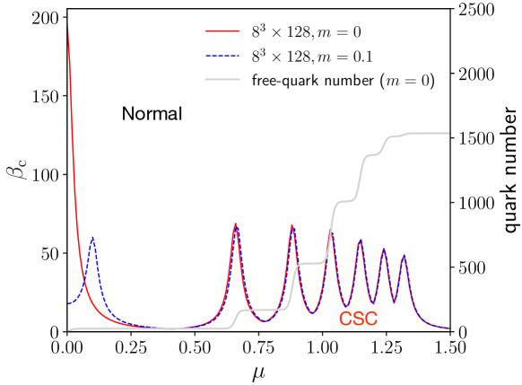
Figure 4: The phase diagram in the $\mu$-$\beta$ plane. The region above the critical coupling $\beta_{c}$ corresponds to the normal phase, whereas the region below $\beta_{c}$ corresponds to the CSC phase. The results for staggered fermions on an $8^{3}\times 128$ lattice with $m=0$ (red solid line) and $m=0.1$ (blue dashed line) are shown. The solid gray line represents the quark number $N_{\rm q}$ for free quarks with $m=0$.

Here we identify the boundary of the normal and CSC phases characterized by $\beta_{c}$ as a function of the quark chemical potential $\mu$ on lattices $L_{s}^{3}\times L_{t}=4^{3}\times 64$, $8^{3}\times 128$ and $16^{3}\times 256$. The chosen aspect ratio $L_{s}/L_{t}=1/16$ is small enough to suppress the thermal fluctuations that may destroy the CSC.

Figure 4 shows the phase diagram in the $\mu$-$\beta$ plane for staggered fermions on an $8^{3}\times 128$ lattice with quark mass $m=0$ and $0.1$ in lattice units. The existence of the CSC is suggested below $\beta_{c}$ although it may be affected by higher order corrections in the small $\beta$ region. The obtained $\beta_{c}$ has many peaks as a function of $\mu$ similarly to the results for the NJL model in a finite box amo02 . Each peak corresponds to the enhancement of the energy gap that occurs when $\mu$ is close to an energy level of the free quark

$$E({\bm{p}})=\sinh^{-1}\sqrt{\sum_{i=1}^{3}\sin^{2}p_{i}+m^{2}}\ ,$$ (14)

where the momentum in the first Brillouin zone is given by

$$\{{\bm{p}}|{\bm{p}}\in{\rm BZ_{\rm s}}\}= \left\{\left.\left(\frac{2\pi n_{1}}{L_{s}},\frac{2\pi n_{2}}{L_{s}},\frac{2\pi n_{3}}{L_{s}}\right)\right|-\frac{L_{s}}{4}\leq n_{i}<\frac{L_{s}}{4},n_{i}\in\mathbb{Z}\right\}\ .$$ (15)

The size of the momentum space is half ($L_{s}/2$) of the spatial lattice size since staggered fermions correspond to Dirac fermions on a coarser lattice with twice as large lattice spacing as the original one. Note that the peak at $\mu=0$ that appears for $m=0$ shifts for finite $m$ to the location corresponding to the lowest energy level $E(\bm{0})=\sinh^{-1}m$. This peak is considered to be a finite-size artifact since it is caused by the condensate of quark-quark and antiquark-antiquark pairs with zero momentum, which vanishes in the thermodynamic limit $L_{s}\rightarrow\infty$.

In Fig. 4 we also plot the quark number for free quarks given by

$$N_{\rm q}=N_{\rm sp}N_{\rm c}N_{\rm f}\sum_{{\bm{p}}\in{\rm BZ}_{\rm s}}\left[n_{\rm F}(E({\bm{p}})-\mu)-n_{\rm F}(E({\bm{p}})+\mu)\right]\ ,$$ (16)

where $N_{\rm sp}=2$, $N_{\rm c}=3$ and $N_{\rm f}=4$ represent the spin, color, and flavor degrees of freedom, respectively, and $n_{\rm F}(x)=[\exp(x/T)+1]^{-1}$ represents the Fermi distribution function at temperature $T$. As $\mu$ increases, the Fermi sphere becomes larger and includes more high-momentum modes, which leads to the stepwise increase of $N_{\rm q}$ matsuoka_thermal_1984 ; i.e., the quark number $N_{\rm q}$ jumps when $\mu$ reaches $\mu=E(\bm{p})$, a discrete energy level of quarks. The critical $\beta_{c}$ has a peak at $\mu$ corresponding to the jump of $N_{\rm q}$. This is consistent with the picture that the condensate is mainly caused by the scattering of fermions near the Fermi surface.

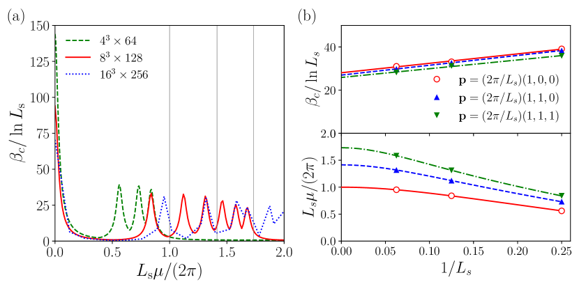
Figure 5: (a) The critical coupling $\beta_{c}$ is plotted against the quark chemical potential $\mu$ for staggered fermions with quark mass $m=0$ on various lattices $L_{s}=4,8,16$ with a fixed aspect ratio $L_{s}/L_{t}=1/16$. Appropriate normalization is used to reveal the expected scaling behavior at large $L_{s}$. The gray vertical lines indicate the expected positions of the peaks in the $L_{s}\to\infty$ limit. (b) The height $\beta_{c}/\ln L_{s}$ and the position $L_{s}\mu/(2\pi)$ of the peaks are plotted against $1/L_{s}$ for momentum modes ${\bm{p}}=(2\pi/L_{s})(1,0,0),\,(2\pi/L_{s})(1,1,0),\,(2\pi/L_{s})(1,1,1)$. The lines in the plot below represent $\mu=E(\bm{p})$.

Next, let us discuss the lattice-size dependence of $\beta_{c}$. By using the dimensional analysis and the $\beta$ function at the one-loop level, we expect a scaling behavior

$$\beta_{c}\sim f\left(\hat{L}\hat{\mu},\hat{L}\hat{T}\right)\ln\left(\frac{1}{a\Lambda_{\rm QCD}}\right)=f\left(L_{s}\mu,\frac{L_{s}}{L_{t}}\right)\ln\left(\frac{L_{s}}{\hat{L}\Lambda_{\rm QCD}}\right)\ ,$$ (17)

where $a$ is the lattice spacing, $f$ is a dimensionless function, while $\hat{L}=aL_{s}$, $\hat{\mu}=\mu/a$ and $\hat{T}=1/(aL_{t})$ are the dimensionful spatial extent, the quark chemical potential, and the temperature, respectively. Eq. (17) suggests

$$\beta_{c}\propto\ln L_{s}$$ (18)

with the dimensionful quantities $\hat{\mu}$, $\hat{T}$ and $\hat{L}$ fixed, or equivalently, $L_{s}\mu$, $L_{s}/L_{t}$ and $\hat{L}$ fixed. Figure 5(a) shows the lattice-size dependence of $\beta_{c}$ for a fixed aspect ratio $L_{s}/L_{t}=1/16$. In Fig. 5(b) we show the $L_{s}$ dependence of the height and the position of the peaks corresponding to the momentum ${\bm{p}}=(2\pi/L_{s})(1,0,0),\,(2\pi/L_{s})(1,1,0),\,(2\pi/L_{s})(1,1,1)$. For all momenta, $\beta_{c}/\ln L_{s}$ depends linearly on $1/L_{s}$ and converges to a finite value as $L_{s}\to\infty$, which suggests that the height of each peak scales as $\ln L_{s}$ for large $L_{s}$. The peak positions agree with $\mu=E({\bm{p}})$ and converge to $L_{s}\mu/(2\pi)=\sqrt{n_{1}^{2}+n_{2}^{2}+n_{3}^{2}}$ ($n_{1,2,3}\in\mathbb{Z}$) as $L_{s}\rightarrow\infty$. In fact, we find that the peak height $\beta_{c}$ at $\mu=0$ is almost independent of $L_{s}$ and it does not follow the scaling (18) unlike the other peaks, which is consistent with our aforementioned interpretation that the peak at $\mu=0$ is merely a finite-size artifact.

3.2 The Cooper pair condensate for staggered fermions

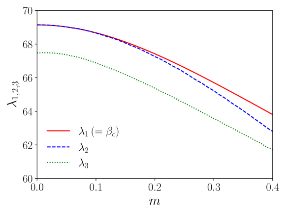
Figure 6: The three largest eigenvalues $\lambda_{1,2,3}$ of $\mathcal{M}$ for staggered fermions on an $8^{3}\times 128$ lattice are plotted against the quark mass $m$ at $\mu=E(|{\bm{p}}|=2\pi/L_{s})$.

Table 1: The irreducible representations of the Euclidean Lorentz group for the Cooper pairs. The condensate and the number of components $N_{\rm comp}$ that correspond to each representation are also shown. We use the Euclidean Dirac gamma matrices $\gamma_{\nu}$, $\gamma_{5}=\gamma_{1}\gamma_{2}\gamma_{3}\gamma_{4}$, $\sigma_{\nu\nu^{\prime}}=(i/2)[\gamma_{\nu},\gamma_{\nu^{\prime}}]$ and the charge conjugation operator $C=\gamma_{2}\gamma_{4}$. Note that $N_{\rm comp}=3$ for $\tilde{S}_{\rm t(pt),\nu\nu^{\prime}}^{fg}(p)$ is obtained from the constraints $\tilde{S}_{\rm t(pt),\nu\nu^{\prime}}^{fg}(p)=-\tilde{S}_{\rm t(pt),\nu^{\prime}\nu}^{fg}(p)$ and $\tilde{S}_{\rm t(pt),\nu_{1}\nu_{2}}^{fg}(p)=(i/2)\epsilon_{\nu_{1}\nu_{2}\nu_{3}\nu_{4}}\tilde{S}_{\rm t(pt),\nu_{3}\nu_{4}}^{fg}(p)$.

representation	condensate	$N_{\rm comp}$
scalar	$\tilde{S}_{\rm s}^{fg}(p)=\epsilon_{ab3}\Braket{\tilde{\psi}_{f}^{a}(p)\Gamma^{\rm s}\tilde{\psi}_{g}^{b}(-p)}$	1
	$\Gamma^{\rm s}=\gamma_{5}C$
pseudo-scalar	$\tilde{S}_{\rm ps}^{fg}(p)=\epsilon_{ab3}\Braket{\tilde{\psi}_{f}^{a}(p)\Gamma^{\rm ps}\tilde{\psi}_{g}^{b}(-p)}$	1
	$\Gamma^{\rm ps}=C$
vector	$\tilde{S}_{\rm v,\nu}^{fg}(p)=\epsilon_{ab3}\Braket{\tilde{\psi}_{f}^{a}(p)\Gamma^{\rm v,\nu}\tilde{\psi}_{g}^{b}(-p)}$	4
	$\Gamma^{\rm v,\nu}=C\gamma_{5}\gamma_{\nu}$
pseudo-vector	$\tilde{S}_{\rm pv,\nu}^{fg}(p)=\epsilon_{ab3}\Braket{\tilde{\psi}_{f}^{a}(p)\Gamma^{\rm pv,\nu}\tilde{\psi}_{g}^{b}(-p)}$	4
	$\Gamma^{\rm pv,\nu}=C\gamma_{\nu}$
self-dual antisymmetric tensor	$\tilde{S}_{\rm t,\nu\nu^{\prime}}^{fg}(p)=\epsilon_{ab3}\Braket{\tilde{\psi}_{f}^{a}(p)\Gamma^{\rm t,\nu\nu^{\prime}}\tilde{\psi}_{g}^{b}(-p)}$	3
	$\Gamma^{\rm t,\nu\nu^{\prime}}=C\gamma_{5}\sigma_{\nu\nu^{\prime}}$
pseudo-self-dual antisymmetric tensor	$\tilde{S}_{\rm pt,\nu\nu^{\prime}}^{fg}(p)=\epsilon_{ab3}\Braket{\tilde{\psi}_{f}^{a}(p)\Gamma^{\rm pt,\nu\nu^{\prime}}\tilde{\psi}_{g}^{b}(-p)}$	3
	$\Gamma^{\rm pt,\nu\nu^{\prime}}=C\sigma_{\nu\nu^{\prime}}$

The Cooper pair condensate at the critical point can be obtained from the eigenvector corresponding to the largest eigenvalue $\beta_{c}$ of $\mathcal{M}$ through Eq. (8) up to an overall factor. We define the Cooper pair condensate in the momentum space as

$$\tilde{S}_{\alpha\beta}^{fg}(p)\equiv\sum_{a,b}\epsilon_{abc}\tilde{S}_{12,(f\alpha)(g\beta)}^{ab}(p)=\sum_{a,b}\epsilon_{abc}\Big{\langle}\tilde{\psi}_{f\alpha}^{a}(p)\tilde{\psi}_{g\beta}^{b}(-p)\Big{\rangle}\ ,$$ (19)

where $\tilde{\psi}_{f\alpha}^{a}(p)$ is the four-flavor Dirac fermion field with the 4d momentum $p=(\bm{p},p_{4})$ constructed from the staggered fermion field with $a$, $f$ and $\alpha$ being the color, flavor and spinor indices, respectively; see Eq. (40). We fix the color index to $c=3$ on the right-hand side of Eq. (19) since the following results do not depend on this choice. We have confirmed that Eq. (19) has large values when $\bm{p}$ satisfies $\mu\approx E(\bm{p})$ and $p_{4}$ is given by the lowest Matsubara frequencies $p_{4}=\pm\pi/L_{t}$ Yokota:2021wwv , which is consistent with the fact that the condensate is formed by quarks with momenta near the Fermi surface.

Since the Cooper pair is a product of two Dirac spinors, it can be decomposed into irreducible representations of the Euclidean Lorentz group as

$$\tilde{S}^{fg}_{\alpha\beta}(p)=\, \frac{1}{4}\Gamma_{\alpha\beta}^{\rm s}\tilde{S}^{fg}_{\rm s}(p)+\frac{1}{4}\Gamma_{\alpha\beta}^{\rm ps}\tilde{S}^{fg}_{\rm ps}(p)+\frac{1}{4}\sum_{\nu}\Gamma_{\alpha\beta}^{\rm v,\nu}\tilde{S}^{fg}_{\rm v,\nu}(p)+\frac{1}{4}\sum_{\nu}\Gamma_{\alpha\beta}^{\rm pv,\nu}\tilde{S}^{fg}_{\rm pv,\nu}(p)$$

$$+\frac{1}{8}\sum_{\nu>\nu^{\prime}}\Gamma_{\alpha\beta}^{\rm t,\nu\nu^{\prime}}\tilde{S}^{fg}_{\rm t,\nu\nu^{\prime}}(p)+\frac{1}{8}\sum_{\nu>\nu^{\prime}}\Gamma_{\alpha\beta}^{\rm pt,\nu\nu^{\prime}}\tilde{S}^{fg}_{\rm pt,\nu\nu^{\prime}}(p)\ ,$$ (20)

where the quantities on the right-hand side are defined in Table 1. Note that $\Gamma_{\alpha\beta}^{\rm s(ps)}$ and $\Gamma_{\alpha\beta}^{\rm t(pt),\nu\nu^{\prime}}$ are anti-symmetric with respect to the exchange of $\alpha$ and $\beta$, while $\Gamma_{\alpha\beta}^{\rm v(pv),\nu}$ are symmetric. Strictly speaking, the Euclidean Lorentz symmetry is broken to the discrete rotational group on the lattice. However, the violation is expected to be small for $\beta_{c}$ at $\mu$ corresponding to the peaks (See the values of $\beta_{c}$ in Fig. 4.). The Dirac gamma matrices are defined, for instance, by

$$\gamma_{i}=\begin{pmatrix}0&i\sigma^{i}\\ -i\sigma^{i}&0\end{pmatrix}\ ,\quad\gamma_{4}=\begin{pmatrix}I_{2}&0\\ 0&-I_{2}\end{pmatrix}$$ (21)

with the Pauli matrices $\sigma^{i}$ and the $2\times 2$ identity matrix $I_{2}$.

To investigate the components of the Cooper pair condensate, we define

$$R_{\rm s(ps)}= \,A\sum_{p,f,g}\left|\tilde{S}^{fg}_{\rm s(ps)}(p)\right|^{2},$$ (22)

$$R_{\rm v(pv)}= \,A\sum_{p,f,g,\nu}\left|\tilde{S}^{fg}_{\rm v(pv),\nu}(p)\right|^{2},$$ (23)

$$R_{\rm t(pt)}= \,\frac{A}{2}\sum_{\nu>\nu^{\prime}}\sum_{p,f,g}\left|\tilde{S}^{fg}_{\rm t(pt),\nu\nu^{\prime}}(p)\right|^{2}\ ,$$ (24)

where $A$ is a normalization factor chosen so that $\sum_{i={\rm s},{\rm ps},{\rm v},{\rm pv},{\rm t},{\rm pt}}R_{i}=1$. The results are almost the same even if we restrict the sum over the momentum to the region $\mu\approx E(\bm{p})$ and $p_{4}=\pm\pi/L_{t}$, where the Cooper pair condensate becomes large.

In Fig. 6 we plot the three largest eigenvalues $\lambda_{1,2,3}$ of $\mathcal{M}$ against the quark mass. As one approaches $m=0$, the two largest eigenvalues come close to each other, which implies the double degeneracy at $m=0$. In Fig. 7 we show the components of the Cooper pair condensate represented by $R_{i}$ for the eigenvectors corresponding to the eigenvalues up to the third largest one for $m=0$. For the two largest eigenvalues, which are degenerate as shown in Fig. 6, we determine the two orthogonal bases of the eigenspace in such a way that either the scalar or the pseudo-scalar component becomes zero. In general, the Cooper pair condensate at the critical point is represented by a linear combination of the scalar and the pseudo-scalar components with the rest of the components being small.

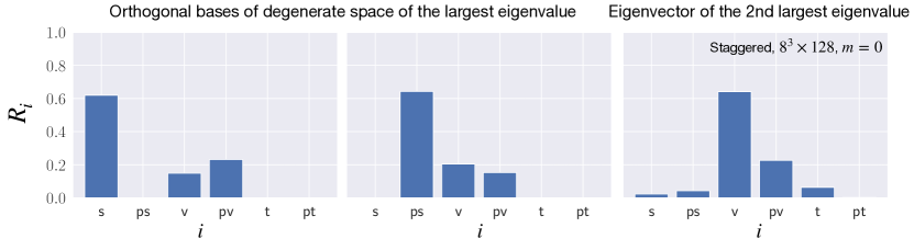
Figure 7: The components of the Cooper pair condensate $R_{i}$ ($i=\mathrm{s},\mathrm{ps},\mathrm{v},\mathrm{pv},\mathrm{t},\mathrm{pt}$) for staggered fermions on an $8^{3}\times 128$ lattice with $m=0$ at $\mu=E(|{\bm{p}}|=2\pi/L_{s})$. The figures on the left and the middle show the results for the two orthogonal bases of the eigenspace of the degenerate two largest eigenvalues $\beta_{c}$ as described in the text. The figure on the right shows the result for the eigenvector corresponding to the third largest eigenvalue.

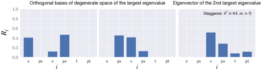
Figure 8: The same as Fig. 7 except that the lattice size is $4^{3}\times 64$.

In Fig. 8 we show the results on a $4^{3}\times 64$ lattice. By comparing them with the results on an $8^{3}\times 128$ lattice in Fig. 7, we observe that the components other than the scalar and the pseudo-scalar are suppressed as the lattice size increases. This suggests that the existence of these components is due to the breaking of the Euclidean Lorentz symmetry by the lattice discretization. The result that the scalar or pseudo-scalar condensate is favored is consistent with the previous work alford_qcd_1998 ; alford_single_2003 ; iwasaki_superconductivity_1995 ; schafer_quark_2000 ; schmitt_when_2002 ; buballa_anisotropic_2003 , which shows that pairing that breaks rotational symmetry is weaker. Similarly, the result of $R_{i}$ for $m=0.4$ is shown in Fig. 9. The degeneracy of the largest eigenvalues is lifted due to the finite mass, and the scalar condensate is favored at the critical point in contrast to the massless case. This is consistent with the common wisdom that the effect of quark mass favors the scalar condensate instead of the pseudo-scalar condensate.

Figure 9: The components of the Cooper pair condensate $R_{i}$ ($i=\mathrm{s},\mathrm{ps},\mathrm{v},\mathrm{pv},\mathrm{t},\mathrm{pt}$) for the eigenvectors corresponding to the eigenvalues up to the third largest one for staggered fermions on an $8^{3}\times 128$ lattice with $m=0.4$ at $\mu=E(|{\bm{p}}|=2\pi/L_{s})$.

Since the scalar and pseudo-scalar condensates are anti-symmetric with respect to the spinor indices, they satisfy

$$\tilde{S}^{fg}_{\rm s(ps)}(p)=-\tilde{S}^{gf}_{\rm s(ps)}(-p)$$ (25)

due to the anti-commuting property of the fermion fields. Eq. (25) can be rewritten as

$$\tilde{S}^{(\pm)fg}_{\rm s(ps)}(p)=\mp\tilde{S}^{(\pm)gf}_{\rm s(ps)}(p)\ ,$$ (26)

where we have defined the spatially symmetric and anti-symmetric components as

$$\tilde{S}^{(\pm)fg}_{\rm s(ps)}(p)=\frac{\tilde{S}^{fg}_{\rm s(ps)}(p)\pm\tilde{S}^{fg}_{\rm s(ps)}(-p)}{2}\ .$$ (27)

In order to determine which component is dominant, we calculate

$$R^{(\pm)}_{\rm s(ps)}=A^{\prime}\sum_{f,g,p}\left|\tilde{S}^{(\pm)fg}_{\rm s(ps)}(p)\right|^{2}\ ,$$ (28)

where $A^{\prime}$ is a normalization factor chosen so that $R^{(+)}_{\rm s(ps)}+R^{(-)}_{\rm s(ps)}=1$. For both the scalar and pseudo-scalar cases, we obtain $R^{(+)}_{\rm s(ps)}\approx 0.71$ for an $8^{3}\times 128$ lattice, which implies that the spatially symmetric component $\tilde{S}^{(+)fg}_{\rm s(ps)}(p)$ is dominant.

Let us also comment (See Ref. Yokota:2021wwv .) that $\tilde{S}^{(+)fg}_{\rm s(ps)}(p)$ do not depend on the direction of $\bm{p}$, which suggests spatially isotropic s-wave superconductivity. Note that the complex phase of $\tilde{S}^{(+)fg}_{\rm s(ps)}(p)$, which is independent of $p$, can take an arbitrary value, reflecting the spontaneous breaking of the $\mathrm{U}_{\rm B}(1)$ baryon-number symmetry $\tilde{\psi}(p)\to e^{i\theta_{\rm B}}\tilde{\psi}(p)$ for $\theta_{\rm B}\in\mathbb{R}$.

Next let us focus on the flavor structure of $\tilde{S}^{(+)fg}_{\rm s(ps)}(p)$. Since it is anti-symmetric with respect to the exchange of $f$ and $g$ as shown in Eq. (26), we can decompose it as

$$\tilde{S}^{(+)fg}_{\rm s(ps)}(p)= \,\tilde{\kappa}_{1,\rm s(ps)}(p)t_{1}^{fg}+\tilde{\kappa}_{3,\rm s(ps)}(p)t_{3}^{fg}+\tilde{\kappa}_{13,\rm s(ps)}(p)\omega_{13}^{fg}+\tilde{\kappa}_{24,\rm s(ps)}(p)\omega_{24}^{fg}$$

$$+\tilde{\kappa}_{25,\rm s(ps)}(p)(t_{2}t_{5})^{fg}+\tilde{\kappa}_{45,\rm s(ps)}(p)(t_{4}t_{5})^{fg},$$ (29)

where $t_{1}$, $t_{3}$, $\omega_{13}$, $\omega_{24}$, $t_{2}t_{5}$ and $t_{4}t_{5}$ are linearly independent anti-symmetric matrices defined through $t_{\mu}={}^{\rm t}\gamma_{\mu}$, $\omega_{\mu\nu}=(i/2)[t_{\mu},t_{\nu}]$, $t_{5}=t_{1}t_{2}t_{3}t_{4}$. We calculate the coefficients $\tilde{\kappa}_{j,\mathrm{s(ps)}}$ numerically for $m=0$ and $m=0.1$ and find

$$\tilde{S}^{(+)fg}_{\rm s}(p)\simeq\tilde{\kappa}_{13,\rm s}(p)\omega_{13}^{fg}\ ,\quad\quad\tilde{S}^{(+)fg}_{\rm ps}(p)\simeq\tilde{\kappa}_{24,\rm ps}(p)\omega_{24}^{fg}\ .$$ (30)

Let us discuss the chiral transformation properties of the Cooper pair condensate $\tilde{S}^{(+)fg}_{\rm s(ps)}(p)$. Here we focus on the $\mathrm{U}_{\rm c}(1)$ chiral symmetry of staggered fermions, which is a remnant of the $\mathrm{SU}_{\rm L}(N_{\rm f})\times\mathrm{SU}_{\rm R}(N_{\rm f})$ chiral symmetry of the continuum theory defined by the transformation

$$\tilde{\psi}(p)\to e^{i\theta_{\rm c}\gamma_{5}\otimes t_{5}}\tilde{\psi}(p)\ ,\quad\quad\theta_{\rm c}\in\mathbb{R}\ ,$$ (31)

where $\gamma_{5}=\gamma_{1}\gamma_{2}\gamma_{3}\gamma_{4}$ and $t_{5}$ act on the spinor and flavor indices, respectively. It is straightforward to derive the transformation

$$\tilde{S}^{(+)fg}_{\alpha\beta}(p)\to\tilde{S}^{(+)fg}_{\alpha\beta}(p)+i\theta_{\rm c}\left(\sum_{f^{\prime},\alpha^{\prime}}t_{5,ff^{\prime}}\gamma_{5,\alpha\alpha^{\prime}}\tilde{S}^{(+)f^{\prime}g}_{\alpha^{\prime}\beta}(p)+\sum_{g^{\prime},\beta^{\prime}}\tilde{S}^{(+)fg^{\prime}}_{\alpha\beta^{\prime}}(p)t_{5,gg^{\prime}}\gamma_{5,\beta\beta^{\prime}}\right)$$ (32)

under Eq. (31) for infinitesimal $\theta_{\rm c}$. By contracting the spinor indices as in Table 1 to extract the scalar and pseudo-scalar components, one obtains the transformation

$$\tilde{S}_{\mathrm{s}}^{(+)fg}(p)\to \tilde{S}_{\mathrm{s}}^{(+)fg}(p)+2i\theta_{\rm c}\tilde{\kappa}_{24,\rm ps}(p)\omega_{13}^{fg}\ ,$$ (33)

$$\tilde{S}_{\mathrm{ps}}^{(+)fg}(p)\to \tilde{S}_{\mathrm{ps}}^{(+)fg}(p)+2i\theta_{\rm c}\tilde{\kappa}_{13,\rm s}(p)\omega_{24}^{fg}\ ,$$ (34)

which amounts to

$$\begin{pmatrix}\tilde{\kappa}_{13,\rm s}(p)\\ \tilde{\kappa}_{24,\rm ps}(p)\end{pmatrix}\to e^{2i\theta_{\rm c}\sigma^{1}}\begin{pmatrix}\tilde{\kappa}_{13,\rm s}(p)\\ \tilde{\kappa}_{24,\rm ps}(p)\end{pmatrix}$$ (35)

for a finite $\theta_{\rm c}$. Thus we find that the Copper pair condensate breaks the $\mathrm{U}_{\rm c}(1)$ chiral symmetry spontaneously, which is reflected in the double degeneracy for $m=0$ in Fig. 6. A finite mass explicitly breaks the symmetry and lifts the degeneracy of the scalar and pseudo-scalar condensates.

In the continuum limit, it is expected that the degeneracy of the largest eigenvalues in the massless case enhances from 2 to 12 due to the recovery of the original $\mathrm{SU}_{\rm L}(4)\times\mathrm{SU}_{\rm R}(4)$ chiral symmetry since there are six ways to select two flavors for anti-commuting indices from four flavors. In other words, all the eigenvalues corresponding to the twelve condensates $\tilde{\kappa}_{1,\mathrm{s(ps)}},\ldots,\tilde{\kappa}_{45,\mathrm{s(ps)}}$ in Eq. (3.2) are expected to degenerate in the continuum limit, which should be seen explicitly by using larger lattices than the ones used in this work.

3.3 Results for Wilson fermions

In this section we present our results for Wilson fermions, which have the advantage of applicability to any number of flavors at the expense of the explicit chiral symmetry breaking. The analysis based on the gap equation is common to all $N_{\rm f}\geq 2$, whereas the single flavor $N_{\rm f}=1$ case has to be treated separately since the absence of the flavor degrees of freedom restricts the possible form of the condensate due to the anti-commutating property of the fermion fields. Here we first discuss the $N_{\rm f}\geq 2$ case comparing the results with those for $N_{\rm f}=4$ staggered fermions, and then discuss the $N_{\rm f}=1$ case.

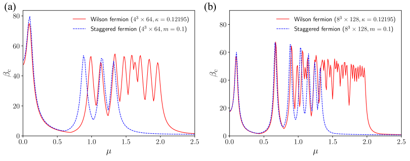
Figure 10: The critical coupling $\beta_{c}$ on (a) $4^{3}\times 64$ and (b) $8^{3}\times 128$ lattices is plotted against the quark chemical potential $\mu$ for $N_{\rm f}\geq 2$ Wilson (red solid lines) and staggered (blue dashed lines) fermions, respectively. The hopping parameter for Wilson fermions is set to $\kappa=0.12195$, which corresponds to $m=0.1$ in the free theory. The mass of staggered fermions is set to $m=0.1$ for comparison.

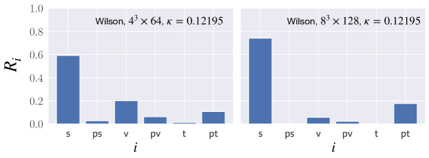
Figure 11: The components of the Cooper pair condensate $R_{i}$ ($i=\mathrm{s},\mathrm{ps},\mathrm{v},\mathrm{pv},\mathrm{t},\mathrm{pt}$) for $N_{\rm f}\geq 2$ Wilson fermions on $4^{3}\times 64$ and $8^{3}\times 128$ lattices with $\kappa=0.12195$ at $\mu=E(|{\bm{p}}|=2\pi/L_{s})$.

Figure 10 shows the critical point $\beta_{c}$ as a function of the quark chemical potential $\mu$ for Wilson fermions together with the result for staggered fermions. Note that the largest eigenvalue $\beta_{c}$ is non-degenerate. Similarly to staggered fermions, we observe a peak structure, where the peak positions correspond to the energy levels $\mu=E({\bm{p}})$ with the dispersion relation

$$E({\bm{p}})=2\sinh^{-1}\sqrt{\frac{\sum_{i=1}^{3}\sin^{2}p_{i}+\left(m+2\sum_{i=1}^{3}\sin^{2}\frac{p_{i}}{2}\right)^{2}}{4\left(1+m+2\sum_{i=1}^{3}\sin^{2}\frac{p_{i}}{2}\right)}}\ .$$ (36)

Here we define $m=1/(2\kappa)-4$ as the quark mass in the free theory with the hopping parameter $\kappa$ and the Wilson parameter $r=1$. The momentum ${\bm{p}}$ is chosen to be in the first Brillouin zone, which is given for Wilson fermions as

$$\{{\bm{p}}|{\bm{p}}\in{\rm BZ_{\rm w}}\}= \left\{\left.\left(\frac{2\pi n_{1}}{L_{s}},\frac{2\pi n_{2}}{L_{s}},\frac{2\pi n_{3}}{L_{s}}\right)\right|-\frac{L_{s}}{2}\leq n_{i}<\frac{L_{s}}{2},n_{i}\in\mathbb{Z}\right\}.$$ (37)

The results for Wilson and staggered fermions agree in the small $\mu$ region, which is understandable since they have the same low-momentum properties with the dispersion relation $E(\bm{p})\approx\sqrt{\bm{p}^{2}+m^{2}}$. Better agreement is observed for the larger lattice, which shifts the peaks towards smaller $\mu$. On the other hand, the results exhibit some discrepancies at large $\mu$. Note, in particular, that the Wilson fermions have additional peaks there, which is understood as a consequence of the difference in the size of the first Brillouin zone (See Eqs. (15) and (37).).

In Fig. 11 we show the components of the Cooper pair condensate by calculating $R_{i}$ ($i={\rm s},{\rm ps},{\rm v},{\rm pv},{\rm t},{\rm pt}$), which are defined in the same manner as in the staggered fermion case (22)–(24). We find that the Cooper pair condensate is of the scalar type, which agrees with the result for staggered fermions with a finite mass.

As in the staggered fermion case, we calculate (28) and find that $R^{(+)}_{\rm s}\approx 0.9997$ for the scalar case with an $8^{3}\times 128$ lattice, which implies that the spatially symmetric component $\tilde{S}^{(+)fg}_{\rm s}(p)$ is dominant. Thus we find that the dominant Cooper pair condensate is anti-symmetric with respect to the flavor indices, which implies two-flavor color superconductivity (2SC) for $N_{\rm f}=2$ and color-flavor locked color superconductivity (CFL) for $N_{\rm f}=3$.

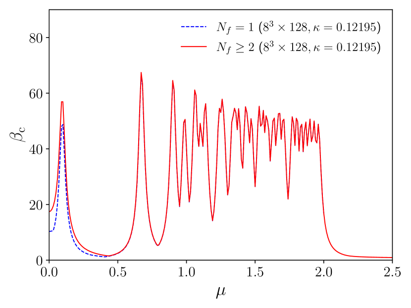
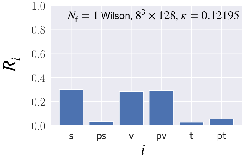
Figure 12: (Left) The critical point $\beta_{c}$ is plotted against the quark chemical potential for Wilson fermions on an $8^{3}\times 128$ lattice with $\kappa=0.12195$. The blue dashed line corresponds to the $N_{\rm f}=1$ case, whereas the red solid line corresponds to the $N_{\rm f}\geq 2$ case. (Right) The components of the Cooper pair condensate $R_{i}$ ($i=\mathrm{s},\mathrm{ps},\mathrm{v},\mathrm{pv},\mathrm{t},\mathrm{pt}$) for $N_{\rm f}=1$ Wilson fermions on an $8^{3}\times 128$ lattice with $\kappa=0.12195$ and $\mu=E(|{\bm{p}}|=2\pi/L_{s})$.

Let us finally comment on the single-flavor case $N_{\rm f}=1$, which is realized by restricting the eigenvector space so that the condensate satisfies the anti-commuting property of the fermion fields without the flavor indices as described in Appendices A.2 and B.1. Figure 12 shows a comparison between $N_{\rm f}=1$ and $N_{\rm f}\geq 2$. From the left panel, we observe that the CSC region shrinks in the $N_{\rm f}=1$ case due to the restriction of the eigenvector space. From the right panel, we find that the scalar component is comparable to the vector and pseudo-vector components unlike the $N_{\rm f}\geq 2$ case. Note here that, in the case of $N_{\rm f}=1$, the scalar condensate is spatially anti-symmetric suggesting the p-wave superconductivity, whereas the vector and pseudo-vector components are spatially symmetric suggesting the s-wave superconductivity. Which is realized in the continuum limit remains to be seen by calculations on a larger lattice. By the same token, the difference of $\beta_{c}$ between the $N_{\rm f}=1$ and $N_{\rm f}\geq 2$ cases, which is visible only for $\mu\lesssim 0.4$ in the left panel, is expected to extend to the larger $\mu$ region in the continuum limit.

4 Summary and discussions

In this paper we provided analytic predictions for the CSC on the lattice, using the fact that the gap equation reduces to a linear equation by focusing on the critical point. In particular, we determined the boundary of the normal and CSC phases in the $\mu$-$\beta$ plane for both staggered and Wilson fermions. The phase boundary shows characteristic peak structure as a function of the quark chemical potential, which is due to the discretization of the quark energy levels in finite systems.

Furthermore, we investigated the form of the Cooper pair condensate at the critical point. In the case of staggered fermions, we observed that the scalar and pseudo-scalar condensates are favored in the massless limit of quarks owing to the $\mathrm{U}_{\rm c}(1)$ chiral symmetry of staggered fermions, which is a remnant of the $\mathrm{SU}_{\rm L}(4)\times\mathrm{SU}_{\rm R}(4)$ chiral symmetry in the continuum. The observed Cooper pair condensate breaks the chiral symmetry spontaneously as well as the $\mathrm{U}_{\rm B}(1)$ baryon-number symmetry. When the quark mass is finite, we found that the degeneracy of the scalar and pseudo-scalar condensates is lifted and that the scalar condensate is favored. From the momentum components of the condensate, we confirmed that spatially isotropic s-wave superconductivity is realized by the Cooper pairs composed of quarks near the Fermi surface. As an extension of this work, it would be interesting to include the chiral condensate, which corresponds to the diagonal components of the Dyson equation in the Nambu-Gor’kov formalism.

In the case of Wilson fermions, we find that the results for $N_{\rm f}\geq 2$ are essentially the same as staggered fermions with a finite mass. In particular, we find that the Cooper pair condensate is anti-symmetric with respect to the flavor indices, which implies 2SC and CFL in the case of $N_{\rm f}=2$ and $N_{\rm f}=3$, respectively. The $N_{\rm f}=1$ case was discussed separately and the results turned out to be different from the $N_{\rm f}\geq 2$ case.

Our results obtained for QCD in a small box provides useful predictions for first-principle calculations based on methods to overcome the sign problem such as the complex Langevin method. Simulations in this direction are ongoing tsutsui_color_2022 ; namekawa_flavor_2022 . Once our predictions are reproduced, the next step would be to make the physical size of the box larger either by decreasing $\beta$ or by using a larger lattice in order to investigate the CSC in a fully non-perturbative regime.

Appendix A Explicit forms of $\mathcal{M}$ for staggered and Wilson fermions

In this Appendix we give the explicit forms of $\mathcal{M}$ for staggered and Wilson fermions. We also make some remarks on the numerical calculation of $\mathcal{M}$.

A.1 Staggered fermions

Here we derive the form of $\mathcal{M}$ in the case of staggered fermions. The action of staggered fermions with mass $m$ and the quark chemical potential $\mu$ in lattice units is given by

$$S =\frac{1}{2}\sum_{n,\nu,a,a^{\prime}}\eta_{\nu}(n)\left\{\overline{\chi}^{a}(n)e^{\delta_{\nu 4}\mu}U_{\nu,aa^{\prime}}(n)\chi^{a^{\prime}}(n+\hat{\nu})-\overline{\chi}^{a}(n-\hat{\nu})e^{-\delta_{\nu 4}\mu}U_{\nu,aa^{\prime}}^{\dagger}(n-\hat{\nu})\chi^{a^{\prime}}(n)\right\}$$

$$\quad+m\sum_{n,a}\overline{\chi}^{a}(n)\chi^{a}(n)+S_{\rm g}\ .$$ (38)

$S_{\rm g}$ is the action for gluons, $n$ is an integer vector labeling the position on the hypercube, $a$ and $b$ are color indices, $\hat{\nu}$ is the unit vector in the $\nu\ (=1,2,3,4)$ direction, $\chi(n)$ and $\overline{\chi}(n)$ are the staggered fermion fields, and $U_{\nu}(n)=e^{ig\sum_{B}A_{\nu}^{B}(n)T^{B}}$ is the link variable related with the gluon field $A_{\nu}^{B}(n)$. We have also introduced the usual site-dependent sign factor $\eta_{\nu}(n)=(-1)^{\sum_{\nu^{\prime}=1}^{\nu-1}n_{\nu^{\prime}}}$. We impose periodic boundary conditions on $\chi(n)$ and $\overline{\chi}(n)$ in the spatial ($\nu=1,2,3$) directions and anti-periodic boundary conditions in the temporal ($\nu=4$) direction. The lattice extent in the $\nu$ direction is denoted by $L_{\nu}$.

First let us derive the Feynman rules for staggered fermions. Following Ref. rot12 , we redefine the fermion field as

$$\chi_{\rho}^{a}(N)=\chi^{a}(2N+\rho)\ ,$$ (39)

where $\rho$ is a four-vector with $\rho_{\nu}=0$ or $1$, while $N$ is a new lattice coordinate labeling the sites on a lattice with twice as large spacing as the original one. This new field (39) is related to the four-flavor Dirac fermion field through

$$\psi_{f\alpha}^{a}(N)\sim\sum_{\rho}(T_{\rho})_{\alpha f}\chi_{\rho}^{a}(N)\ ,$$ (40)

where $\alpha$ and $f$ are the spinor and flavor indices, respectively, and $T_{\rho}$ is defined by

$$T_{\rho}=\gamma_{1}^{\rho_{1}}\gamma_{2}^{\rho_{2}}\gamma_{3}^{\rho_{3}}\gamma_{4}^{\rho_{4}}$$ (41)

with $\gamma_{\mu}$ being the Euclidean Dirac gamma matrices. In terms of $\chi_{\rho}^{a}(N)$, the free part of the action is written as

$$S_{\rm f}^{\rm free}= \sum_{N,N^{\prime},\rho,\rho^{\prime},a,a^{\prime}}\overline{\chi}^{a}_{\rho}(N)D_{\rho\rho^{\prime}}^{aa^{\prime}}(N-N^{\prime})\chi_{\rho^{\prime}}^{a^{\prime}}(N^{\prime})\ ,$$ (42)

$$D_{\rho\rho^{\prime}}^{aa^{\prime}}(N)= \delta_{a,a^{\prime}}\sum_{\nu}\frac{\eta_{\nu}(\rho)}{2}\left\{e^{\delta_{\nu 4}\mu}(\delta_{\rho+\hat{\nu},\rho^{\prime}}\delta_{N,0}+\delta_{\rho-\hat{\nu},\rho^{\prime}}\delta_{N+\hat{\nu},0})\right.$$

$$-\left.e^{-\delta_{\nu 4}\mu}(\delta_{\rho-\hat{\nu},\rho^{\prime}}\delta_{N,0}+\delta_{\rho+\hat{\nu},\rho^{\prime}}\delta_{N-\hat{\nu},0})\right\}+\tilde{m}_{\rm q}\delta_{a,a^{\prime}}\delta_{\rho\rho^{\prime}}\delta_{N,0}\ ,$$ (43)

where $\eta_{\nu}(2N+\rho)=\eta_{\nu}(\rho)$ has been used. Let us switch to the momentum representation by using the Fourier transformation

$$\tilde{f}(p)= \sum_{N}e^{-ip\cdot(2N)}f(N)\quad\quad\text{for }f=\chi_{\rho}^{a},\,\overline{\chi}_{\rho}^{a}\ ,$$ (44)

and restrict the range of momentum $p$ to the first Brillouin zone

$$\{p|p\in{\rm BZ_{\rm s}}\}= \left\{\left.\left(\frac{2\pi n_{1}}{L_{1}},\frac{2\pi n_{2}}{L_{2}},\frac{2\pi n_{3}}{L_{3}},\frac{(2n_{4}+1)\pi}{L_{4}}\right)\right|-\frac{L_{\nu}}{4}\leq n_{\nu}<\frac{L_{\nu}}{4},n_{\nu}\in\mathbb{Z}\right\}\ ,$$ (45)

using the periodicity $\tilde{f}(p+\pi\hat{\nu})=\tilde{f}(p)$. Eq. (42) can then be written in the momentum representation as

$$S_{\rm f}^{\rm free}= \sum_{p\in{\rm BZ}_{\rm s}}\sum_{\rho,\rho^{\prime},a,a^{\prime}}\tilde{\overline{\chi}}^{a}_{\rho}(p)\tilde{D}_{\rho\rho^{\prime}}^{aa^{\prime}}(p)\tilde{\chi}_{\rho^{\prime}}^{a^{\prime}}(-p)\ ,$$ (46)

$$\tilde{D}_{\rho\rho^{\prime}}^{aa^{\prime}}(p)= \delta_{aa^{\prime}}\left(\sum_{\nu}i\Gamma^{\nu}_{\rho\rho^{\prime}}(2p)\sin\overline{p}_{\nu}+m\delta_{\rho\rho^{\prime}}\right)\ ,$$ (47)

from which we obtain the fermion propagator

$$\tilde{D}_{\rho\rho^{\prime}}^{-1,aa^{\prime}}(p)=\delta_{aa^{\prime}}\tilde{D}_{\rho\rho^{\prime}}^{-1}(p)=\delta_{aa^{\prime}}\frac{-\sum_{\nu}i\Gamma^{\nu}_{\rho\rho^{\prime}}(2p)\sin\overline{p}_{\nu}+m\delta_{\rho\rho^{\prime}}}{\sum_{\nu}\sin^{2}\overline{p}_{\nu}+m^{2}}\ .$$ (48)

Here we have introduced $\overline{p}_{\nu}=p_{\nu}-i\mu\delta_{\nu 4}$ and

$$\Gamma^{\nu}_{\rho\rho^{\prime}}(2p)=e^{ip\cdot(\rho-\rho^{\prime})}(\delta_{\rho+\hat{\nu},\rho^{\prime}}+\delta_{\rho-\hat{\nu},\rho^{\prime}})\eta_{\nu}(\rho)\ ,$$ (49)

which satisfies the same algebra as the Dirac gamma matrices as $\{\Gamma^{\nu}(2p),\Gamma^{\nu^{\prime}}(2p)\}_{\rho\sigma}=2\delta_{\nu\nu^{\prime}}\delta_{\rho\sigma}$.

By expanding $U_{\nu}(n)=e^{ig\sum_{B}A_{\nu}^{B}(n)T^{B}}$ with respect to $g$, we obtain the interaction term

$$S_{\rm f}^{\rm int}= ig\sum_{N,N^{\prime},\rho,\rho^{\prime},a,a^{\prime},B}\overline{\chi}^{a}_{\rho}(N)\sum_{\nu}\frac{\eta_{\nu}(\rho)}{2}$$

$$\times\left\{e^{\delta_{\nu 4}\mu}A_{\nu}^{B}(2N+\rho)T^{B}_{aa^{\prime}}(\delta_{\rho+\hat{\nu},\rho^{\prime}}\delta_{N,N^{\prime}}+\delta_{\rho-\hat{\nu},\rho^{\prime}}\delta_{N+\hat{\nu},N^{\prime}})\right.$$

$$-\left.e^{-\delta_{\nu 4}\mu}A_{\nu}^{B}(2N+\rho-\hat{\nu})T^{B}_{aa^{\prime}}(\delta_{\rho-\hat{\nu},\rho^{\prime}}\delta_{N,N^{\prime}}+\delta_{\rho+\hat{\nu},\rho^{\prime}}\delta_{N-\hat{\nu},N^{\prime}})\right\}\chi_{\rho^{\prime}}^{a^{\prime}}(N^{\prime})+\mathcal{O}(g^{2})\ ,$$ (50)

which can be rewritten in the momentum space as

$$S_{\rm f}^{\rm int}= \frac{1}{V^{\prime}V}\sum_{k\in{\rm BZ}_{\rm g}}\sum_{p\in{\rm BZ}_{\rm s}}\sum_{\rho,\rho^{\prime},a,a^{\prime},B,\nu}ig\Pi_{\rho\rho^{\prime},aa^{\prime}}^{B\nu}(p,k)\tilde{\overline{\chi}}^{a}_{\rho}(-p)\tilde{A}_{\nu}^{B}(-k)\tilde{\chi}^{a^{\prime}}_{\rho^{\prime}}(p+k)\ ,$$ (51)

using the three-point vertex $\Pi_{\rho\rho^{\prime},aa^{\prime}}^{B\nu}(p,k)$ given by

$$\Pi_{\rho\rho^{\prime},aa^{\prime}}^{B\nu}(p,k)= e^{-ik\cdot\rho}\cos\left(\overline{p}_{\nu}+\frac{{k}_{\nu}}{2}\right)\Gamma^{\nu}_{\rho\rho^{\prime}}\left(2(p+k)\right)T^{B}_{aa^{\prime}}\ .$$ (52)

Here we have introduced the momentum representation for the gluon field rot12 as

$$A^{B}_{\nu}(n)=\frac{1}{V}\sum_{k\in{\rm BZ}_{\rm g}}e^{ik\cdot n+ik_{\nu}/2}\tilde{A}^{B}_{\nu}(k)\ ,$$ (53)

where $V=L_{1}L_{2}L_{3}L_{4}$ and

$$\{k|k\in{\rm BZ}_{\rm g}\}=\left\{\left.\left(\frac{2\pi n_{1}}{L_{1}},\frac{2\pi n_{2}}{L_{2}},\frac{2\pi n_{3}}{L_{3}},\frac{2\pi n_{4}}{L_{4}}\right)\right|-\frac{L_{\nu}}{2}\leq n_{\nu}<\frac{L_{\nu}}{2},n_{\nu}\in\mathbb{Z}\right\}.$$ (54)

Note that the range of momentum in the first Brillouin zone is different from Eq. (45) for the fermion field. The gluon propagator is given by rot12

$$G_{\nu\nu^{\prime}}^{BB^{\prime}}(k)= \frac{\delta_{BB^{\prime}}}{\tilde{k}^{2}}\left\{\delta_{\nu\nu^{\prime}}-(1-\alpha_{0})\frac{\tilde{k}_{\nu}\tilde{k}_{\nu^{\prime}}}{\tilde{k}^{2}}\right\}=G(k)\delta_{BB^{\prime}}\left\{\delta_{\nu\nu^{\prime}}-(1-\alpha_{0})\frac{\tilde{k}_{\nu}\tilde{k}_{\nu^{\prime}}}{\tilde{k}^{2}}\right\}\ ,$$ (55)

where $\tilde{k}_{\nu}=2\sin(k_{\nu}/2)$ and $\alpha_{0}$ is the gauge parameter. Since the results are independent of the choice of $\alpha_{0}$ at the one-loop level, we choose the Feynman gauge $\alpha_{0}=1$ for simplicity.

$$=\delta_{aa^{\prime}}\tilde{D}_{\rho\rho^{\prime}}^{-1}(p)=\delta_{aa^{\prime}}\frac{-\sum_{\nu}i\Gamma^{\nu}_{\rho\rho^{\prime}}(2p)\sin\overline{p}_{\nu}+m\delta_{\rho\rho^{\prime}}}{\sum_{\nu}\sin^{2}\overline{p}_{\nu}+m^{2}}$$

$$=\delta_{BB^{\prime}}\delta_{\nu\nu^{\prime}}G(k)=\delta_{BB^{\prime}}\delta_{\nu\nu^{\prime}}\frac{1}{4\sum_{\nu^{\prime\prime}}\sin^{2}\left(\frac{k_{\nu^{\prime\prime}}}{2}\right)}$$

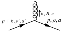
$$=igT_{aa^{\prime}}^{B}\Pi_{\rho\rho^{\prime}}^{\nu}(p,k)=igT^{B}_{aa^{\prime}}e^{-ik\cdot\rho}\cos\left(\overline{p}_{\nu}+\frac{{k}_{\nu}}{2}\right)\Gamma^{\nu}_{\rho\rho^{\prime}}\left(2(p+k)\right)$$

Figure 13: Feynman rules for staggered fermions used in our calculation.

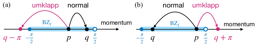
Figure 14: One-dimensional illustration of the two possible scatterings in the cases of (a) $p\leq q$ and (b) $q<p$ for the fermion momenta $p$ and $q$.

Figure 13 summarizes the Feynman rules used in our calculation. The other terms, such as the multi-gluon vertices, contribute only to higher-order corrections and hence are ignored in our calculation. Using these rules, we obtain $\mathcal{M}$ defined in Fig. 2(b) as

$$\mathcal{M}_{(p\rho\rho^{\prime})(q\sigma\sigma^{\prime})}= \frac{N_{\rm c}+1}{V}\sum_{\nu,\gamma,\gamma^{\prime}}\sum_{k\in{\rm BZ}_{\rm g}}\tilde{\delta}_{q-p-k}^{\rm F}G(k)$$

$$\times\Pi_{\rho\gamma}^{\nu}(p,k)\tilde{D}_{\gamma\sigma}^{-1}(p+k)\Pi_{\rho^{\prime}\gamma^{\prime}}^{\nu}(-p,-k)\tilde{D}_{\gamma^{\prime}\sigma^{\prime}}^{-1}(-p-k)\ .$$ (56)

Here we have introduced the periodic delta function

$$\tilde{\delta}_{k}^{\rm F}=\begin{cases}1&(k_{1,\cdots,4}\in\pi\mathbb{Z})\\ 0&(\text{otherwise})\ ,\end{cases}$$ (57)

which has the period $\pi$ in each direction inherited from that of $\mathrm{BZ}_{\mathrm{f}}$ in (45). It should be noted that the difference in the size of the first Brillouin zone between fermions and gluons allows two scattering processes, namely the normal and umklapp scatterings, in each direction for any $p$ and $q$. Figure 14 is a one-dimensional illustration of these processes. Due to the range of the gluon momentum $-\pi\leq k<\pi$, not only the normal process but also the umklapp process, where $p+k$ exceeds the domain of the first Brillouin zone, always occurs for any fermion momenta. In four dimensions, the existence of both scatterings in each direction is represented by the solution of $\tilde{\delta}_{q-p-k}^{\rm F}=1$ in $-\pi\leq k_{\nu}<\pi$ given by

$$k_{\nu}= q_{\nu}-p_{\nu}-\pi\rho^{\prime\prime}_{\nu}\,{\rm sgn}_{+}(q_{\nu}-p_{\nu})\quad(\rho^{\prime\prime}_{\nu}=0,1)$$ (58)

with

$${\rm sgn}_{+}(x)=\begin{cases}1&\mbox{~{}for~{}}x\geq 0\\ -1&\mbox{~{}for~{}}x<0\ .\end{cases}$$ (59)

After performing the sum over $k$ in Eq. (56), we obtain

$$\mathcal{M}_{(p\rho\rho^{\prime})(q\sigma\sigma^{\prime})}= \frac{N_{\rm c}+1}{V}\sum_{\nu,\gamma,\gamma^{\prime}}\sum_{\rho^{\prime\prime}}G\left(k(q,p,\rho^{\prime\prime})\right)\Pi_{\rho\gamma}^{\nu}\left(p,k(q,p,\rho^{\prime\prime})\right)\tilde{D}_{\gamma\sigma}^{-1}(p+k(q,p,\rho^{\prime\prime}))$$

$$\times\Pi_{\rho^{\prime}\gamma^{\prime}}^{\nu}\left(-p,-k(q,p,\rho^{\prime\prime})\right)\tilde{D}_{\gamma^{\prime}\sigma^{\prime}}^{-1}(-p-k(q,p,\rho^{\prime\prime}))\ ,$$ (60)

where $k(q,p,\rho^{\prime\prime})$ is defined by Eq. (58). In the case of Wilson fermions discussed in the following subsection, only one of the normal and umklapp scatterings occurs for a given momentum transfer because there is no difference in the first Brillouin zone between fermions and gluons.

A.2 Wilson fermions

Next let us derive the form of $\mathcal{M}$ in the case of Wilson fermions, where the fermion fields on the lattice site $N$ are denoted by $\psi^{a}_{f\alpha}(N)$ and $\overline{\psi}^{a}_{f\alpha}(N)$ with $a$, $f$ and $\alpha$ being the color, flavor and spinor indices, respectively. The action is given by

$$S= \frac{1}{2}\sum_{N,a,a^{\prime},\alpha,\alpha^{\prime},f,\nu}\left\{\overline{\psi}^{a}_{f\alpha}(N)(\gamma_{\nu})_{\alpha\alpha^{\prime}}e^{\mu\delta_{\nu 4}}U_{\nu,aa^{\prime}}(N)\psi^{a^{\prime}}_{f\alpha^{\prime}}(N+\hat{\nu})\right.$$

$$\left.\qquad\qquad\qquad\,-\overline{\psi}^{a}_{f\alpha}(N+\hat{\nu})(\gamma_{\nu})_{\alpha\alpha^{\prime}}e^{-\mu\delta_{\nu 4}}U_{\nu,aa^{\prime}}^{\dagger}(N)\psi^{a^{\prime}}_{f\alpha^{\prime}}(N)\right\}+m\sum_{N,a,\alpha,f}\overline{\psi}^{a}_{f\alpha}(N)\psi_{f\alpha}^{a}(N)$$

$$-\frac{r}{2}\sum_{N,a,a^{\prime},\alpha,f,\nu}\left\{\overline{\psi}^{a}_{f\alpha}(N)e^{\mu\delta_{\nu 4}}U_{\nu,aa^{\prime}}(N)\psi^{a^{\prime}}_{f\alpha}(N+\hat{\nu})\right.$$

$$\left.\qquad\qquad\qquad\,-2\overline{\psi}^{a}_{f\alpha}(N)\delta_{a,a^{\prime}}\psi^{a^{\prime}}_{f\alpha}(N)+\overline{\psi}^{a}_{f\alpha}(N+\hat{\nu})e^{-\mu\delta_{\nu 4}}U_{\nu,aa^{\prime}}^{\dagger}(N)\psi^{a^{\prime}}_{f\alpha}(N)\right\}+S_{\rm g}\ ,$$ (61)

where $m$ and $\mu$ are the mass and the quark chemical potential in lattice units, respectively, and $r$ is the Wilson parameter, which defines the hopping parameter as $\kappa=1/(2m+8r)$.

$$=\delta_{aa^{\prime}}\delta_{ff^{\prime}}\tilde{D}_{\alpha\alpha^{\prime}}^{-1}(p)=\delta_{aa^{\prime}}\delta_{ff^{\prime}}\frac{-\sum_{\nu}i\gamma^{\nu}_{\alpha\alpha^{\prime}}\sin\overline{p}_{\nu}+M(\overline{p})\delta_{\alpha\alpha^{\prime}}}{\sum_{\nu}\sin^{2}\overline{p}_{\nu}+M(\overline{p})^{2}}$$

$$=\delta_{BB^{\prime}}\delta_{\nu\nu^{\prime}}G(k)=\delta_{BB^{\prime}}\delta_{\nu\nu^{\prime}}\frac{1}{4\sum_{\nu^{\prime\prime}}\sin^{2}\left(\frac{k_{\nu^{\prime\prime}}}{2}\right)}$$

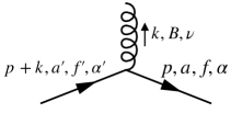
$$=-ig\delta_{ff^{\prime}}T^{B}_{aa^{\prime}}\Pi^{\nu}_{\alpha\alpha^{\prime}}(q,q^{\prime})$$

$$=-ig\delta_{ff^{\prime}}T^{B}_{aa^{\prime}}\left(\gamma_{\nu,\alpha\alpha^{\prime}}\cos\frac{\overline{q}_{\nu}^{{}^{\prime}}-\overline{q}_{\nu}^{*}}{2}-\delta_{\alpha\alpha^{\prime}}ir\sin\frac{\overline{q}_{\nu}^{{}^{\prime}}-\overline{q}_{\nu}^{*}}{2}\right)$$

Figure 15: Feynman rules for Wilson fermions used in our calculation. We have introduced $\overline{q}_{\nu}=q_{\nu}-i\mu\delta_{\nu 4}$ and $M(\overline{p})=m+2r\sum_{\nu}\sin^{2}(\overline{p}_{\nu}/2)$.

Similarly to staggered fermions, the Feynman rules are derived from the action rot12 . In Fig. 15 we summarize the Feynman rules in the momentum space used in our calculation. According to these rules, $\mathcal{M}$ is evaluated as

$$\mathcal{M}_{(pf\alpha f^{\prime}\alpha^{\prime}),(qh\beta h^{\prime}\beta^{\prime})}= \delta_{fh}\delta_{f^{\prime}h^{\prime}}\frac{N_{\rm c}+1}{V}G(q-p)\sum_{\gamma,\gamma^{\prime},\mu}\Pi_{\alpha^{\prime}\gamma^{\prime}}^{\mu}(-p,q)\tilde{D}^{-1}_{\gamma^{\prime}\beta^{\prime}}(q)\Pi_{\alpha\gamma}^{\mu}(p,-q)\tilde{D}^{-1}_{\gamma\beta}(-q)$$ (62)

with $V=L_{1}L_{2}L_{3}L_{4}$. As for the indices of $\mathcal{M}$, let us recall that the indices $\rho$, $\rho^{\prime}$, $\sigma$ and $\sigma^{\prime}$ used in Sec. 2 represent the flavor and spinor indices collectively. The first Brillouin zone for Wilson fermions is given by the momentum region

$$\{p|p\in{\rm BZ_{\rm w}}\}=\left\{\left.\left(\frac{2\pi n_{1}}{L_{1}},\frac{2\pi n_{2}}{L_{2}},\frac{2\pi n_{3}}{L_{3}},\frac{2\pi n_{4}}{L_{4}}\right)\right|-\frac{L_{\nu}}{2}\leq n_{\nu}<\frac{L_{\nu}}{2},n_{\nu}\in\mathbb{Z}\right\}\ .$$ (63)

Since $\mathcal{M}$ trivially acts on the flavor indices, i.e., $\mathcal{M}_{(pf\alpha f^{\prime}\alpha^{\prime}),(qh\beta h^{\prime}\beta^{\prime})}\propto\delta_{fh}\delta_{f^{\prime}h^{\prime}}$, the largest eigenvalue is independent of $N_{\rm f}$ as far as the number of flavors is $N_{\rm f}\geq 2$. For the single flavor case $N_{\rm f}=1$, however, the largest eigenvalue can be different because of the restriction on the eigenvectors $\tilde{\Sigma}^{(-)}_{12(pf\alpha f^{\prime}\alpha^{\prime})}$ due to the anti-commuting property of the fermion fields (See Appendix B.1.). Namely, since $\tilde{\Sigma}^{(-)}_{12(pf\alpha f^{\prime}\alpha^{\prime})}=\tilde{\Sigma}^{(-)}_{12(p\alpha\alpha^{\prime})}$, the eigenvector must satisfy $\tilde{\Sigma}^{(-)}_{12(p\alpha\alpha^{\prime})}=\tilde{\Sigma}^{(-)}_{12(-p\alpha^{\prime}\alpha)}$ because of Eq. (66). This is in contrast to the multi-flavor case, where more general types of condensate are allowed since $\tilde{\Sigma}^{(-)}_{12(pf\alpha f^{\prime}\alpha^{\prime})}$ can be anti-symmetric with respect to the flavor indices $f$ and $f^{\prime}$.

A.3 Some remarks on the calculation of $\mathcal{M}$

Here we make some remarks on the numerical calculation of $\mathcal{M}$ that applies to both staggered and Wilson fermions. First we point out that the elements corresponding to zero momentum transfer diverge due to $G(0)$, which is the contribution from the gluon zero modes. This is an artifact of perturbation theory on a finite lattice, which disappears in the large volume limit. Note also that the divergence does not appear in non-perturbative treatments (See Ref. Asano:2023nef , for instance.). In this work, we simply omit the contribution from $G(0)$ by hand.

The next point concerns the memory consumption by $\mathcal{M}$, which is a huge and dense matrix. For instance, for staggered fermions, the number of elements is $256V^{2}$ for the lattice volume $V$, which amounts to $18{\rm TB}$ for $V=8^{3}\times 128$ with double precision complex numbers. Therefore, keeping all the elements in the memory is not practical. Instead, we decompose $\mathcal{M}$ into parts whose memory consumption is at most $O(V)$, such as $G$ and $\tilde{D}^{-1}$ in Eq. (A.1), and calculate the elements of $\mathcal{M}$ from these parts every time they are needed.

Appendix B Details of the power iteration method

B.1 Initial condition for the power iteration

In the power iteration method, one extracts the largest eigenvalue and the corresponding eigenvector by multiplying $\mathcal{M}$ many times to a randomly selected initial vector. However, in order to obtain eigenvectors with appropriate symmetry properties, one needs to impose some condition on the initial vector.

Note that the anomalous propagator for fermions $\tilde{S}_{12,\rho\rho^{\prime}}^{(aa^{\prime})}(p)=\langle\tilde{\psi}^{a}_{\rho}(p)\tilde{\psi}^{a^{\prime}}_{\rho^{\prime}}(-p)\rangle$ satisfies the relation

$$\tilde{S}_{12,\rho\rho^{\prime}}^{aa^{\prime}}(p)=-\tilde{S}_{12,\rho^{\prime}\rho}^{a^{\prime}a}(-p)\ .$$ (64)

Similarly, the anomalous self-energy satisfies

$$\tilde{\Sigma}_{12,\rho\rho^{\prime}}^{aa^{\prime}}(p)=-\tilde{\Sigma}_{12,\rho^{\prime}\rho}^{a^{\prime}a}(-p)\ ,$$ (65)

as one can see from Eq. (5). Therefore, we have

$$\tilde{\Sigma}_{12(p\rho\rho^{\prime})}^{(-)}=\tilde{\Sigma}_{12(-p\rho^{\prime}\rho)}^{(-)}$$ (66)

for $\tilde{\Sigma}_{12(p\rho\rho^{\prime})}^{(-)}$ in Eq. (12).

Let us decompose the vector space $\mathcal{V}$ on which $\mathcal{M}$ acts as $\mathcal{V}=\mathcal{V}_{\rm F}+\mathcal{V}_{\rm B}$, where $\mathcal{V}_{\rm F(B)}$ is the vector space whose elements satisfy

$$v_{(q\rho\rho^{\prime})}= v_{(-q\rho^{\prime}\rho)}\quad \text{for }v\in\mathcal{V}_{\rm F}\ ,$$ (67)

$$v_{(q\rho\rho^{\prime})}= -v_{(-q\rho^{\prime}\rho)}\quad \text{for }v\in\mathcal{V}_{\rm B}\ .$$ (68)

By using the relation

$$\mathcal{M}_{(p\rho\rho^{\prime})(q\sigma\sigma^{\prime})}=\mathcal{M}_{(-p\rho^{\prime}\rho)(-q\sigma^{\prime}\sigma)}\ ,$$ (69)

which is obtained from the representation in Fig. 2(b), one can show that

$$\mathcal{M}v\in\mathcal{V}_{\rm F}\quad \text{if }v\in\mathcal{V}_{\rm F}\ ,$$ (70)

$$\mathcal{M}v\in\mathcal{V}_{\rm B}\quad \text{if }v\in\mathcal{V}_{\rm B}\ ,$$ (71)

which implies that $\mathcal{V}_{\rm F}$ and $\mathcal{V}_{\rm B}$ are not mixed by multiplying $\mathcal{M}$. Therefore, the initial vector must satisfy Eq. (67) in order to obtain the eigenvector satisfying Eq. (66).

The eigenvalue equation for Wilson fermions reduces to

$$\sum_{q\beta\beta^{\prime}}\mathcal{M}_{(p\alpha\alpha^{\prime})(q\beta\beta^{\prime})}^{\prime}\tilde{\Sigma}^{(-)}_{12(qf\beta f^{\prime}\beta^{\prime})}=\beta\,\tilde{\Sigma}^{(-)}_{12(pf\alpha f^{\prime}\alpha^{\prime})}\ ,$$ (72)

where $\mathcal{M}^{\prime}$ is related to $\mathcal{M}$ given by Eq. (62) as

$$\mathcal{M}_{(pf\alpha f^{\prime}\alpha^{\prime}),(qh\beta h^{\prime}\beta^{\prime})}=\delta_{fh}\delta_{f^{\prime}h^{\prime}}\mathcal{M}_{(p\alpha\alpha^{\prime}),(q\beta\beta^{\prime})}^{\prime}\ .$$

As we mentioned in Appendix A.2, the allowed forms of the eigenvector $\tilde{\Sigma}^{(-)}_{12(pf\alpha f^{\prime}\alpha^{\prime})}$ are different between the single- and multi-flavor cases for Wilson fermions. Let us decompose $\tilde{\Sigma}^{(-)}_{12(pf\alpha f^{\prime}\alpha^{\prime})}$ into the symmetric and antisymmetric parts with respect to $f$ and $f^{\prime}$. Abbreviating the flavor indices, we denote the former and latter parts by $\tilde{\Sigma}^{(-+)}_{12(p\alpha\alpha^{\prime})}$ and $\tilde{\Sigma}^{(--)}_{12(p\alpha\alpha^{\prime})}$, respectively. In the single-flavor case, $\tilde{\Sigma}^{(--)}_{12(q\beta\beta^{\prime})}$ does not exist, which forces us to choose the initial vector to satisfy the condition

$$\tilde{\Sigma}^{(-+)}_{12(q\beta\beta^{\prime})} =\tilde{\Sigma}^{(-+)}_{12(-q\beta^{\prime}\beta)}$$ (73)

due to Eq. (66).

B.2 Extension to the second and the third largest eigenvalues

In this section we extend the power iteration method to the calculation of the second and the third largest eigenvalues as well as the corresponding eigenvectors. Let us assume that the largest eigenvalue $\lambda_{1}$ and the corresponding eigenvector $v_{1}$ of $\mathcal{M}$ defined in Fig. 2(b) are obtained. If one defines $\tilde{v}$ by projecting out the $v_{1}$ component from $v$ and applies the power iteration to $\tilde{v}$, the second largest eigenvalue $\lambda_{2}$ and the corresponding eigenvector $v_{2}$ are obtained. By repeating this procedure, one obtains the third largest one as well.

If $\mathcal{M}$ were Hermitian, the projection can be made by using the orthogonality of the eigenvectors. In fact, $\mathcal{M}$ is not Hermitian but pseudo-Hermitian dir42 ; pauli_diracs_1943 ; lee_negative_1969

$$\mathcal{M}_{(p\rho\rho^{\prime})(q\sigma\sigma^{\prime})}^{\dagger}=\left[\eta\mathcal{M}\eta^{-1}\right]_{(p\rho\rho^{\prime})(q\sigma\sigma^{\prime})}$$ (74)

with a Hermitian matrix $\eta$ for both staggered and Wilson fermions.

In order to make the projection in this case, we need to consider the relationship among the eigenvectors under the condition (74). Let $\lambda_{n}$ and $v_{n}$ be an eigenvalue and the corresponding eigenvector, respectively, with the ordering $|\lambda_{1}|\geq|\lambda_{2}|\geq\cdots$. The eigenvalue equation reads

$$\mathcal{M}v_{n}= \lambda_{n}v_{n}\ .$$ (75)

By using its Hermitian conjugate and Eq. (74), we obtain

$$v_{n}^{\dagger}\eta\mathcal{M}=\lambda_{n}^{*}v_{n}^{\dagger}\eta\ .$$ (76)

Acting this on $v_{m}$ and using Eq. (75), we have

$$(\lambda_{m}-\lambda_{n}^{*})v_{n}^{\dagger}\eta v_{m}=0\ .$$ (77)

From this, we find that the eigenvalue $\lambda_{n}$ is real if $v_{n}^{\dagger}\eta v_{n}\neq 0$ and that the eigenvectors satisfy $v_{n}^{\dagger}\eta v_{m}=0$ if $\lambda_{m}\neq\lambda_{n}^{*}$, which can be regarded as a generalization of the properties in the Hermitian case.

Suppose we have already obtained $v_{1},v_{2},\ldots,v_{m-1}$ for an integer $m\geq 1$, which satisfy $v_{n}^{\dagger}\eta v_{n}\neq 0$ and $v_{n}^{\dagger}\eta v_{n^{\prime}}=0$ for all $n,n^{\prime}<m$. Then we can get rid of these components as

$$\tilde{v}=v-\sum_{n<m}a_{n}v_{n}\ ,$$ (78)

where the coefficient $a_{n}$ for $n<m$ is given by

$$a_{n}=\frac{v^{\dagger}_{n}\eta v}{v^{\dagger}_{n}\eta v_{n}}\ .$$ (79)

As mentioned above, we can extract $\lambda_{m}$ and $v_{m}$ by applying the power iteration to $\tilde{v}$. As far as $v_{n}^{\dagger}\eta v_{n}\neq 0$ is satisfied for the obtained eigenvectors, we can repeat the procedure to extract other eigenvalues and eigenvectors. In the process of our calculations, we checked $v_{n}^{\dagger}\eta v_{n}\neq 0$ for the obtained eigenvectors.

References

- (1) G. Odyniec, Probing the QCD Phase Diagram with Heavy-Ion Collision Experiments, in Understanding the Origin of Matter, D. Blaschke, K. Redlich, C. Sasaki and L. Turko, eds., vol. 999, pp. 3–29, Springer International Publishing (2022), DOI.
- (2) M.G. Orsaria, G. Malfatti, M. Mariani, I.F. Ranea-Sandoval, F. García, W.M. Spinella et al., Phase transitions in neutron stars and their links to gravitational waves, J. Phys. G 46 (2019) 073002 [1907.04654].
- (3) K. Nagata, Finite-density lattice QCD and sign problem: Current status and open problems, Prog. Part. Nucl. Phys. 127 (2022) 103991 [2108.12423].
- (4) G. Parisi, On complex probabilities, Phys. Lett. 131B (1983) 393.
- (5) J.R. Klauder, Coherent-state langevin equations for canonical quantum systems with applications to the quantized hall effect, Phys. Rev. A 29 (1984) 2036.
- (6) G. Aarts, E. Seiler and I.-O. Stamatescu, The Complex Langevin method: When can it be trusted?, Phys. Rev. D81 (2010) 054508 [0912.3360].
- (7) G. Aarts, F.A. James, E. Seiler and I.-O. Stamatescu, Complex langevin: Etiology and diagnostics of its main problem, Eur.Phys.J.C 71 (2011) 1756 [1101.3270].
- (8) K. Nagata, J. Nishimura and S. Shimasaki, Justification of the complex Langevin method with the gauge cooling procedure, PTEP 2016 (2016) 013B01 [1508.02377].
- (9) K. Nagata, J. Nishimura and S. Shimasaki, Argument for justification of the complex Langevin method and the condition for correct convergence, Phys. Rev. D94 (2016) 114515 [1606.07627].
- (10) E. Witten, Analytic continuation of Chern-Simons theory, AMS/IP Stud. Adv. Math. 50 (2011) 347 [1001.2933].
- (11) AuroraScience collaboration, New approach to the sign problem in quantum field theories: High density qcd on a lefschetz thimble, Phys.Rev.D 86 (2012) 074506 [1205.3996].
- (12) M. Cristoforetti, F. Di Renzo, A. Mukherjee and L. Scorzato, Monte Carlo simulations on the Lefschetz thimble: Taming the sign problem, Phys. Rev. D 88 (2013) 051501 [1303.7204].
- (13) H. Fujii, D. Honda, M. Kato, Y. Kikukawa, S. Komatsu and T. Sano, Hybrid monte carlo on lefschetz thimbles - a study of the residual sign problem, JHEP 10 (2013) 147 [1309.4371].
- (14) A. Alexandru, G. Basar, P.F. Bedaque, G.W. Ridgway and N.C. Warrington, Sign problem and monte carlo calculations beyond lefschetz thimbles, JHEP 05 (2016) 053 [1512.08764].
- (15) M. Fukuma and N. Umeda, Parallel tempering algorithm for integration over Lefschetz thimbles, PTEP 2017 (2017) 073B01 [1703.00861].
- (16) M. Fukuma and N. Matsumoto, Worldvolume approach to the tempered Lefschetz thimble method, PTEP 2021 (2021) 023B08 [2012.08468].
- (17) M. Fukuma, N. Matsumoto and Y. Namekawa, Statistical analysis method for the worldvolume hybrid Monte Carlo algorithm, PTEP 2021 (2021) 123B02 [2107.06858].
- (18) G. Fujisawa, J. Nishimura, K. Sakai and A. Yosprakob, Backpropagating Hybrid Monte Carlo algorithm for fast Lefschetz thimble calculations, JHEP 04 (2022) 179 [2112.10519].
- (19) Y. Mori, K. Kashiwa and A. Ohnishi, Toward solving the sign problem with path optimization method, Phys. Rev. D 96 (2017) 111501 [1705.05605].
- (20) Y. Mori, K. Kashiwa and A. Ohnishi, Application of a neural network to the sign problem via the path optimization method, PTEP 2018 (2018) 023B04 [1709.03208].
- (21) A. Alexandru, P.F. Bedaque, H. Lamm and S. Lawrence, Finite-Density Monte Carlo Calculations on Sign-Optimized Manifolds, Phys. Rev. D 97 (2018) 094510 [1804.00697].
- (22) M. Levin and C.P. Nave, Tensor renormalization group approach to 2d classical lattice models, Phys.Rev.Lett. 99 (2007) 120601 [cond-mat/0611687].
- (23) D. Sexty, Simulating full QCD at nonzero density using the complex Langevin equation, Phys. Lett. B 729 (2014) 108 [1307.7748].
- (24) G. Aarts, E. Seiler, D. Sexty and I.-O. Stamatescu, Simulating QCD at nonzero baryon density to all orders in the hopping parameter expansion, Phys. Rev. D90 (2014) 114505 [1408.3770].
- (25) Z. Fodor, S. Katz, D. Sexty and C. Torok, Complex Langevin dynamics for dynamical QCD at nonzero chemical potential: A comparison with multiparameter reweighting, Phys. Rev. D 92 (2015) 094516 [1508.05260].
- (26) K. Nagata, J. Nishimura and S. Shimasaki, Complex Langevin calculations in finite density QCD at large /T with the deformation technique, Phys. Rev. D 98 (2018) 114513 [1805.03964].
- (27) J.B. Kogut and D.K. Sinclair, Applying Complex Langevin Simulations to Lattice QCD at Finite Density, Phys. Rev. D 100 (2019) 054512 [1903.02622].
- (28) D. Sexty, Calculating the equation of state of dense quark-gluon plasma using the complex Langevin equation, Phys. Rev. D 100 (2019) 074503 [1907.08712].
- (29) M. Scherzer, D. Sexty and I.O. Stamatescu, Deconfinement transition line with the complex Langevin equation up to , Phys. Rev. D 102 (2020) 014515 [2004.05372].
- (30) Y. Ito, H. Matsufuru, Y. Namekawa, J. Nishimura, S. Shimasaki, A. Tsuchiya et al., Complex Langevin calculations in QCD at finite density, JHEP 10 (2020) 144 [2007.08778].
- (31) F. Attanasio, B. Jäger and F.P.G. Ziegler, QCD equation of state via the complex Langevin method, 2203.13144.
- (32) S. Tsutsui, Y. Asano, Y. Ito, H. Matsufuru, Y. Namekawa, J. Nishimura et al., Color superconductivity in a small box: a complex Langevin study, PoS LATTICE2021 (2022) 533 [2111.15095].
- (33) Y. Namekawa, Y. Asano, Y. Ito, T. Kaneko, H. Matsufuru, J. Nishimura et al., Flavor number dependence of QCD at finite density by the complex Langevin method, PoS LATTICE2021 (2022) 623 [2112.00150].
- (34) B.C. Barrois, Superconducting quark matter, Nucl. Phys. B 129 (1977) 390.
- (35) S.C. Frautschi, Asymptotic Freedom and Color Superconductivity in Dense Quark Matter, in Hadronic Matter at Extreme Energy Density, N. Cabibbo and L. Sertorio, eds., (Boston, MA), pp. 19–27, Springer US (1980), DOI.
- (36) D. Bailin and A. Love, Superfluidity in Ultrarelativistic Quark Matter, Nucl. Phys. B 190 (1981) 175.
- (37) M.G. Alford, K. Rajagopal and F. Wilczek, QCD at finite baryon density: Nucleon droplets and color superconductivity, Phys. Lett. B 422 (1998) 247 [hep-ph/9711395].
- (38) S. Hands, T.J. Hollowood and J.C. Myers, Numerical Study of the Two Color Attoworld, JHEP 12 (2010) 057 [1010.0790].
- (39) S. Hands, T.J. Hollowood and J.C. Myers, QCD with Chemical Potential in a Small Hyperspherical Box, JHEP 07 (2010) 086 [1003.5813].
- (40) S. Hands and D.N. Walters, Evidence for BCS diquark condensation in the (3+1)-d lattice NJL model, Phys. Lett. B 548 (2002) 196 [hep-lat/0209140].
- (41) M.G. Alford, A. Schmitt, K. Rajagopal and T. Schäfer, Color superconductivity in dense quark matter, Rev. Mod. Phys. 80 (2008) 1455.
- (42) W.E. Brown, J.T. Liu and H.-c. Ren, The transition temperature to the superconducting phase of QCD at high baryon density, Phys. Rev. D 62 (2000) 054016 [hep-ph/9912409].
- (43) T. Yokota, Y. Asano, Y. Ito, H. Matsufuru, Y. Namekawa, J. Nishimura et al., Perturbative predictions for color superconductivity on the lattice, PoS LATTICE2021 (2022) 562 [2111.14578]. (Comment: The result for Wilson fermions on a lattice was presented already in this proceedings article as Fig. 4. However, we found a mistake in the code used to generate that figure. The result after correction is shown in Fig. 10 of the present paper.)
- (44) L.G. Moretto, Pairing fluctuations in excited nuclei and the absence of a second order phase transition, Phys. Lett. B 40 (1972) 1.
- (45) A.L. Goodman, Statistical fluctuations in the i132 model, Phys. Rev. C 29 (1984) 1887.
- (46) R. Rossignoli, N. Canosa and P. Ring, Effective mean field approximation in hot finite systems, Phys. Rev. Lett. 72 (1994) 4070.
- (47) Y. Nambu, Quasi-particles and gauge invariance in the theory of superconductivity, Phys. Rev. 117 (1960) 648.
- (48) D.J. Thouless, Perturbation theory in statistical mechanics and the theory of superconductivity, Annals Phys. 10 (1960) 553.
- (49) P. Amore, M.C. Birse, J.A. McGovern and N.R. Walet, Color superconductivity in finite systems, Phys. Rev. D 65 (2002) 074005 [hep-ph/0110267].
- (50) H. Matsuoka and M. Stone, Thermal Distribution Functions and Finite Size Effects for Lattice Fermions, Phys. Lett. B 136 (1984) 204.
- (51) M.G. Alford, J.A. Bowers, J.M. Cheyne and G.A. Cowan, Single color and single flavor color superconductivity, Phys. Rev. D 67 (2003) 054018 [hep-ph/0210106].
- (52) M. Iwasaki and T. Iwado, Superconductivity in the quark matter, Phys. Lett. B 350 (1995) 163.
- (53) T. Schäfer, Quark hadron continuity in QCD with one flavor, Phys. Rev. D 62 (2000) 094007 [hep-ph/0006034].
- (54) A. Schmitt, Q. Wang and D.H. Rischke, When the transition temperature in color superconductors is not like in BCS theory, Phys. Rev. D 66 (2002) 114010 [nucl-th/0209050].
- (55) M. Buballa, J. Hosek and M. Oertel, Anisotropic admixture in color superconducting quark matter, Phys. Rev. Lett. 90 (2003) 182002 [hep-ph/0204275].
- (56) H.J. Rothe, Lattice Gauge Theories, World Scientific, 4th ed. (2012), 10.1142/8229, [https://www.worldscientific.com/doi/pdf/10.1142/8229].
- (57) Y. Asano and J. Nishimura, The dynamics of zero modes in lattice gauge theory—difference between SU(2) and SU(3) in 4D, 2303.01008.
- (58) P.A.M. Dirac, Bakerian lecture - the physical interpretation of quantum mechanics, Proceedings of the Royal Society of London. Series A. Mathematical and Physical Sciences 180 (1942) 1 [https://royalsocietypublishing.org/doi/pdf/10.1098/rspa.1942.0023].
- (59) W. Pauli, On dirac’s new method of field quantization, Rev. Mod. Phys. 15 (1943) 175.
- (60) T.D. Lee and G.C. Wick, Negative Metric and the Unitarity of the S Matrix, Nucl. Phys. B 9 (1969) 209.