Defining eccentricity for gravitational wave astronomy

Abstract

Eccentric compact binary mergers are significant scientific targets for current and future gravitational wave observatories. To detect and analyze eccentric signals, there is an increasing effort to develop waveform models, numerical relativity simulations, and parameter estimation frameworks for eccentric binaries. Unfortunately, current models and simulations use different internal parameterisations of eccentricity in the absence of a unique natural definition of eccentricity in general relativity, which can result in incompatible eccentricity measurements. In this paper, we adopt a standardized definition of eccentricity and mean anomaly based solely on waveform quantities, and make our implementation publicly available through an easy-to-use Python package, gw_eccentricity. This definition is free of gauge ambiguities, has the correct Newtonian limit, and can be applied as a postprocessing step when comparing eccentricity measurements from different models. This standardization puts all models and simulations on the same footing and enables direct comparisons between eccentricity estimates from gravitational wave observations and astrophysical predictions. We demonstrate the applicability of this definition and the robustness of our implementation for waveforms of different origins, including post-Newtonian theory, effective one body, extreme mass ratio inspirals, and numerical relativity simulations. We focus on binaries without spin-precession in this work, but possible generalizations to spin-precessing binaries are discussed.

I Introduction

The gravitational wave (GW) detectors LIGO Aasi et al. (2015) and Virgo Acernese et al. (2015) have observed a total of $\mathchar 21016\relax\,90$ compact binary coalescences so far Abbott et al. (2021a), which includes binary black holes (BHs) Abbott et al. (2016), binary neutron stars (NSs) Abbott et al. (2017a) and BH-NS binaries Abbott et al. (2021b). One of the key goals of GW astronomy is to understand how such compact binaries form in nature. The astrophysical source properties inferred from the GW signals carry valuable clues about the origin of these binaries. In particular, the spins of the compact objects and the eccentricity of the orbit are powerful GW observables for this purpose.

If the spins are aligned with the orbital angular momentum, the orbital plane remains fixed throughout the evolution. If the spins are tilted on the other hand, the spins interact with the orbit, causing the orbital plane to precess on a timescale of several orbits Apostolatos et al. (1994); Kidder (1995). Spin-precession leaves a direct imprint on the GW signal and can be used to distinguish between possible binary formation mechanisms. For example, while isolated binaries formed in galactic fields are expected to have aligned spins Mapelli (2020), binaries formed via random encounters in dense stellar clusters can have randomly oriented spins Mapelli (2020). To reliably extract this astrophysical information from GW signals, accurate waveform models Varma et al. (2019a); Pratten et al. (2021); Ossokine et al. (2020); Gamba et al. (2022); Estellés et al. (2022); Hamilton et al. (2021) and GW data analysis methods Farr et al. (2014); Romero-Shaw et al. (2020a); Veitch et al. (2015) that capture the effects of spin-precession have been developed.

By contrast, orbital eccentricity leads to bursts of GW radiation at every pericenter (point of closest approach) passage Peters and Mathews (1963); Peters (1964), which appear as orbital timescale modulations of the GW amplitude and frequency Blanchet (2014). The eccentricity of GW signals carries information about the binary formation mechanism that is complimentary to what can be learned from spin-precession alone. For example, isolated galactic-field binaries are expected to become circularized via GW emission Peters and Mathews (1963); Peters (1964) before they enter the LIGO-Virgo frequency band Mapelli (2020). Because eccentric signals are considered less likely for LIGO-Virgo, most analyses to date (e.g. Ref. Abbott et al. (2021a)) ignore eccentricity. However, binaries formed via random encounters in dense clusters can merge before they can circularize, thereby entering the LIGO-Virgo band with a finite eccentricity Mapelli (2020). Similarly, in hierarchical triple systems, the tidal effect of the tertiary can excite periodic eccentricity oscillations of the inner binary Naoz (2016), resulting in high-eccentricity mergers in the LIGO-Virgo band Martinez et al. (2020).

LIGO-Virgo observations can be used to ascertain whether the assumptions of small eccentricity are valid, and to measure any nonzero eccentricity that may be present. Therefore, eccentricity measurements and/or upper limits from GW signals are highly sought after, and several groups have already analysed the observed signals to obtain information on eccentricity Romero-Shaw et al. (2019, 2020b); Gayathri et al. (2022); Calderón Bustillo et al. (2021a, b); O’Shea and Kumar (2021); Gamba et al. (2023); Romero-Shaw et al. (2022). As LIGO-Virgo, now joined by KAGRA Akutsu et al. (2021), continue to improve Abbott et al. (2018), and with next-generation ground-based detectors expected in the 2030s Punturo et al. (2010); Hild et al. (2011); Abbott et al. (2017b); Reitze et al. (2019), future observations will enable stronger constraints on eccentricity.

The case for eccentric signals is stronger for the future space-based GW observatory LISA, which will see the earlier inspiral phase of some of the BH mergers observed by LIGO-Virgo Sesana (2016); Seoane et al. (2023); Klein et al. (2022), at which point they may still have larger eccentricity. Furthermore, mergers of supermassive black hole binaries observed by LISA may have significant eccentricity if triple dynamics played a role in overcoming the final parsec problem Bonetti et al. (2018). Finally, LISA will observe the mergers of stellar mass compact objects with supermassive black holes, the so-called extreme mass ratio inspirals (EMRIs). EMRIs are expected to primarily be formed through dynamical capture leading to high eccentricities when entering the LISA band Seoane et al. (2023).

Driven by these observational prospects, there has been an increasing effort to develop waveform models Warburton et al. (2012); Osburn et al. (2016); Cao and Han (2017); Liu et al. (2020); Ramos-Buades et al. (2022a); Nagar et al. (2021); Islam et al. (2021); Liu et al. (2022); Memmesheimer et al. (2004); Huerta et al. (2014); Tanay et al. (2016); Cho et al. (2022); Moore et al. (2018); Moore and Yunes (2019); van de Meent and Warburton (2018); Chua et al. (2021); Hughes et al. (2021); Katz et al. (2021); Lynch et al. (2022); Klein (2021), gravitational self-force calculations Barack and Sago (2010); Akcay et al. (2013); Hopper and Evans (2013); Osburn et al. (2014); van de Meent and Shah (2015); Hopper et al. (2016); Forseth et al. (2016); van de Meent (2016, 2018); Munna et al. (2020); Munna and Evans (2020, 2022a, 2022b), numerical relativity (NR) simulations Hinder et al. (2018); Boyle et al. (2019); Ramos-Buades et al. (2022b); Healy and Lousto (2022); Habib and Huerta (2019); Huerta et al. (2019); Joshi et al. (2023), and source parameter estimation methods Abbott et al. (2017c); Lower et al. (2018); Ramos-Buades et al. (2020a); Romero-Shaw et al. (2019, 2020b); Gayathri et al. (2022); Ramos-Buades et al. (2020b); Calderón Bustillo et al. (2021a, b); O’Shea and Kumar (2021); Gamba et al. (2023); Romero-Shaw et al. (2023, 2022); Knee et al. (2022); Bonino et al. (2023); Klein et al. (2022); Yang et al. (2022) that include the effects of eccentricity. In addition to these efforts, one important obstacle needs to be overcome in order to reliably extract eccentricity from GW signals: Eccentricity is not uniquely defined in general relativity Blanchet (2014), and therefore most waveform models and simulations use custom internal definitions that rely on gauge-dependent quantities like binary orbital parameters or compact object trajectories. As a result, the eccentricity inferred from GW signals can be riddled with ambiguity and can even be incompatible between different models Knee et al. (2022). Such ambiguities propagate into any astrophysical applications, including using eccentricity to identify the binary formation mechanism. To resolve this problem, there is a need for a standardized definition of eccentricity for GW applications.

In addition to eccentricity, one needs two more parameters to fully describe an eccentric orbit – one describing the current position of the bodies on the orbit relative to the previous pericenter passage and the other describing the size of the orbit. Mean anomaly Blanchet (2014); Schmidt et al. (2017); Islam et al. (2021), which is the fraction of the orbital period (expressed as an angle) that has elapsed since the last pericenter passage, can be used as the first parameter.  The size of the eccentric orbit can be described, for example, by the semi-major axis $a$ which is related to the orbital period $P$ as $a^{3}\propto P^{2}$ for a Keplerian orbit. For general relativistic orbits, the orbital period decreases as the binary inspirals, while the frequency increases. While the GW frequency itself can be nonmonotonic for eccentric binaries, as we will discuss in Sec. II.5, one can construct an orbit-averaged frequency that is monotonically increasing. Using such an orbit-averaged frequency one can construct a one-to-one map between the orbit-averaged frequency and the orbital period (and therefore the semi-major axis). Thus a reference frequency like the orbital-averaged frequency can be used to describe the size of the orbit.

A good definition of eccentricity should have the following features:

1. To fully describe an eccentric orbit at a given reference frequency, two parameters are required: eccentricity and mean anomaly. Therefore, the definition should include both eccentricity and mean anomaly.

2. To avoid gauge ambiguities, eccentricity and mean anomaly should be defined using only observables at future null-infinity, like the gravitational waveform.

3. In the limit of large binary separation, the eccentricity should approach the Newtonian value, which is uniquely defined.

4. The standardized definition should be applicable over the full range of allowed eccentricities for bound orbits ($0-1$). It should return zero for quasicircular inspirals and limit to one for marginally bound “parabolic” trajectories.

5. Because the eccentricity and mean anomaly vary during a binary’s evolution, one must pick a point in the evolution at which to measure them. This is generally taken to be the point where the GW frequency reaches a certain reference value $f_{\text{ref}}$ (typically 20Hz Abbott et al. (2021a)). However, because eccentricity causes modulations in the GW frequency, the same $f_{\text{ref}}$ can occur at multiple points. Therefore, the standardized definition should also prescribe how to select an unambiguous reference point for eccentric binaries.

6. As current GW detectors are only sensitive to frequencies above a certain $f_{\text{low}}$ (typically 20Hz Abbott et al. (2021a)), when using time-domain waveforms, one typically discards all times below $t_{\text{low}}$, chosen so that the GW frequency crosses 20Hz at $t_{\text{low}}$. Once again, because the GW frequency is nonmonotonic, the standardized definition should prescribe how to select $t_{\text{low}}$ for eccentric binaries.

Additionally, the following features, while not strictly required, can be important for practical applications:

1. In the limit of large mass ratio, the eccentricity should approach the test particle eccentricity on a Kerr geodesic. Since the geodesic eccentricity is not uniquely defined, it is not strictly required that the standard definition of eccentricity matches the geodesic eccentricity defined in any particular coordinates. As described in Sec. IV.1, the definition adopted in this work only approximately matches the geodesic eccentricity defined in the Boyer–Lindquist coordinates.

2. The eccentricity and mean anomaly computation should be computationally inexpensive and robust across binary parameter space and be applicable to a broad range of waveform models and NR simulations. Thus, most models/simulations can continue to rely on their internal eccentricity definitions as it is most convenient to conduct source parameter estimation using the internal definitions. However, if the computation is cheap and robust, one can convert posterior samples from the internal definition to the standardized one as a postprocessing step, thus putting all models and simulations on the same footing.

In this paper, we adopt a standardized eccentricity and mean anomaly definition that meets all of the criteria in the first list of (required) features and also satisfies the criteria in the second list of (desired but not strictly required) features to a great extent. Over the last few years, there have been several attempts to standardize the definition of eccentricity Ramos-Buades et al. (2020a); Islam et al. (2021); Ramos-Buades et al. (2020a); Bonino et al. (2023), or map between different definitions Knee et al. (2022), but these approaches either ignore mean anomaly, or do not have the correct limits at large separation or large mass ratio Ramos-Buades et al. (2022b). More recently, Ref. Ramos-Buades et al. (2022b) introduced a new definition, that has the correct limits, which we adopt in this work. We rigorously test and demonstrate the robustness of our implementation on eccentric waveforms spanning the full range of eccentricities and different origins: post-Newtonian (PN) theory, NR, effective one body (EOB), and EMRIs.

While we focus on eccentric binaries without spin-precession for simplicity, we include a discussion of how our methods can be extended to spin-precessing eccentric systems. In addition, we describe how $f_{\text{ref}}$ and $t_{\text{low}}$ should be generalized for eccentric binaries, along with a discussion on the benefit of using dimensionless reference points Varma et al. (2022a). Our computation is very cheap, and our implementation can be used directly during source parameter estimation or as a postprocessing step. We make our implementation publicly available through an easy-to-use Python package gw_eccentricity Shaikh et al. .

This paper is organized as follows. In Sec. II, we describe the standardized eccentricity and mean anomaly definitions, along with a discussion of how to generalize $f_{\text{ref}}$ and $f_{\text{low}}$. In Sec. III, we provide implementation details, along with different choices for capturing the eccentricity modulations in waveforms. In Sec. IV, we demonstrate the robustness of our implementation on waveforms of different origins and over the full range of eccentricities. We finish with some concluding remarks in Sec. V.

II Defining eccentricity

II.1 Notation and conventions

The component masses of a binary are denoted as $m_{1}$ and $m_{2}$, with $m_{1}\geq m_{2}$, total mass $M=m_{1}+m_{2}$, and mass ratio $q=m_{1}/m_{2}\geq 1$. The dimensionless spin vectors of the component objects are denoted as $\bm{\chi}_{1}$ and $\bm{\chi}_{2}$, and have a maximum magnitude of 1. For binaries without spin-precession, the direction of the orbital angular momentum $\bm{L}$ is fixed, and is aligned to the $z$-axis by convention. For these binaries, the spins are constant and are aligned or anti-aligned to $\bm{L}$, meaning that the only nonzero spin components are $\chi_{1z}$ and $\chi_{2z}$.

The plus ($h_{+}$) and cross ($h_{\!\times\!}$) polarizations of GWs can be conveniently represented by a single complex time series $\mathpzc{h}=h_{+}-i\,h_{\!\times\!}$. The complex waveform on a sphere can be decomposed into a sum of spin-weighted spherical harmonic modes $\mathpzc{h}_{\ell m}$, so that the waveform along any direction $(\iota,\varphi_{0})$ in the binary’s source frame is given by

$$\mathpzc{h}(t,\iota,\varphi_{0})=\sum_{\ell=2}^{\ell=\infty}\sum_{m=-\ell}^{m=\ell}\mathpzc{h}_{\ell m}(t)\leavevmode\nobreak\ {}_{-2}Y_{\ell m}(\iota,\,\varphi_{0}),$$ (1)

where $\iota$ and $\varphi_{0}$ are the polar and azimuthal angles on the sky in the source frame, and ${}_{-2}Y_{\ell m}$ are the spin$=-2$ weighted spherical harmonics. Unless the total mass and/or distance are explicitly specified, we work with the waveform at future null-infinity scaled to unit total mass and distance for simplicity. We also shift the time array of the waveform such that $t=0$ occurs at the peak of the amplitude of the dominant $(2,2)$ mode.  We note, however, that the implementation in gw_eccentricity Shaikh et al. handles waveforms in arbitrary units and time conventions.

II.2 Eccentricity definitions used in PN, EOB, self-force and NR

Because eccentricity is not uniquely defined in general relativity, a wide variety of definitions of eccentricity exists. At Newtonian order, eccentricity can be uniquely defined as Goldstein et al. (2002).

$$e_{\text{Newt}}=\frac{r^{\text{a}}-r^{\text{p}}}{r^{\text{a}}+r^{\text{p}}},$$ (2)

where $r^{\text{a}}$ and $r^{\text{p}}$ are the separations at apocenter (point of furthest approach) and pericenter (point of closest approach), respectively. Starting at 1PN order, the Keplerian parametrization can be extended to the so-called quasi-Keplerian parametrization where three different eccentricity parameters are defined, the radial $e_{r}$, temporal $e_{t}$ and angular $e_{\phi}$ eccentricities, each of which has the same Newtonian limit Blanchet (2014). These quantities can be defined in terms of the conserved energy and angular momentum, but depend on the gauge used Memmesheimer et al. (2004).

The Bondi energy and angular momentum of a binary can be accessed from the metric at future null-infinity and are (nearly) gauge invariant. One might therefore hope to formulate a definition of eccentricity based purely on these two quantities that satisfies all of our requirements. Unfortunately, this will be challenging for the following reasons: Suppose we define eccentricity as some function $e(E,J)$ of the Bondi energy $E$ and angular momentum $J$. The equation $e=0$ will generically define a 1-dimensional subset of the $(E,J)$-plane, which would be shared by all quasicircular inspirals. However, the track followed by a quasicircular binary through the $(E,J)$-plane depends on the mass ratio and the spins (e.g. see Ref. Ossokine et al. (2018)). Consequently, a definition of eccentricity based purely on $E$ and $J$ cannot assign zero eccentricity to all quasicircular inspirals, i.e. it cannot satisfy requirement (D) above.

One might further hope to overcome this by adding an explicit dependence on the mass ratio and spins to the definition. But this cannot account for the fact that different inspiral models will, in general, still not agree on the location of the $e=0$ locus. Consequently, whatever reference model is chosen as the basis for the definition, it will be unable to assign zero eccentricity to quasicircular inspirals produced by all models. This is made worse by the fact that the $e=0$ locus represents the edge of the allowable range of $E$ and $J$; if the values of $E$ and $J$ for some model lie outside the range of the reference model (e.g. see ef. Ramos-Buades et al. (2022b)), analytically inverting the relationship with $e$ would assign a complex value to $e$.

Finally, one might hope to cure this behaviour by basing the definition of $e$ on $E-E_{\text{qc}}$, where $E_{\text{qc}}$ is the energy of the quasicircular counterpart with same angular momentum (and mass-ratio and spins) as the model being measured. However, $E_{\text{qc}}$ is not something that can be inferred from observables at null-infinity (violating requirement (B)). Furthermore, $E_{\text{qc}}$ may not be straightforward to obtain in some models (e.g. numerical relativity), unless one relies on a reference model, which comes with the problems noted above. We, therefore, do not take this approach. Similar objections arise with gauge invariant definitions of eccentricity based on the radial and azimuthal periods, as are commonly used to facilitate gauge invariant comparisons between self-force and PN results for eccentric orbits Barack and Sago (2011); Akcay et al. (2015, 2017).

In the EOB formalism, initial conditions for the dynamics are prescribed in terms of an eccentricity parameter defined within the quasi-Keplerian parameterization Hinderer and Babak (2017); Chiaramello and Nagar (2020); Khalil et al. (2021); Nagar et al. (2021); Ramos-Buades et al. (2022a). Thus, the gauge dependency of the eccentricity parameter also extends to the EOB waveforms Ramos-Buades et al. (2022a); Nagar et al. (2021). In self-force calculations for EMRIs, one typically uses an eccentricity definition based on the turning points of the underlying geodesics Warburton et al. (2012); Osburn et al. (2016); van de Meent and Warburton (2018); Chua et al. (2021); Hughes et al. (2021); Katz et al. (2021); Lynch et al. (2022). This is inherently dependent on the coordinates used for the background spacetime, and picks-up further gauge ambiguities at higher orders in the mass ratio. For NR waveforms, the compact object trajectories are used to define eccentricity, typically by fitting to analytical PN (or Newtonian) expressions Buonanno et al. (2011); Mroue and Pfeiffer (2012); Ramos-Buades et al. (2019); Ciarfella et al. (2022). This also inherently depends on the gauge employed in the simulations.

II.3 Defining eccentricity using the waveform

A more convenient definition of eccentricity that can be straightforwardly applied to waveforms of all origins was proposed in Ref. Mora and Will (2002):

$$e_{\Omega_{\text{orb}}}(t)=\frac{\sqrt{\Omega^{\text{p}}_{\text{orb}}(t)}-\sqrt{\Omega^{\text{a}}_{\text{orb}}(t)}}{\sqrt{\Omega^{\text{p}}_{\text{orb}}(t)}+\sqrt{\Omega^{\text{a}}_{\text{orb}}(t)}},$$ (3)

where $\Omega^{\text{p}}_{\text{orb}}(t)$ is an interpolant through the orbital frequency $\Omega_{\text{orb}}(t)$ evaluated at pericenter passages, and likewise for $\Omega^{\text{a}}_{\text{orb}}(t)$ at apocenter passages. Because eccentricity causes a burst of radiation at pericenters, the times corresponding to pericenters are identified as local maxima in $\Omega_{\text{orb}}(t)$, while apocenters are identified as local minima. Eq. (3) was used, for example, in Ref. Lewis et al. (2017) to analyze generic spin-precessing and eccentric binary BH waveforms. Unfortunately, because $\Omega_{\text{orb}}$ is computed using the compact object trajectories, Eq. (3) is also susceptible to gauge choices, especially for NR simulations.

Nevertheless, Eq. (3) has the important quality that it can be applied to waveforms of all origins. Furthermore, Eq. (3) has the correct Newtonian limit. This is easily seen using Kepler’s second law $\Omega_{\text{orb}}\propto 1/r^{2}$, where $r$ is the binary separation Goldstein et al. (2002); Kep . Using this relation in Eq. (3), one finds that $e_{\Omega_{\text{orb}}}$ matches $e_{\text{Newt}}$ from Eq. (2).

The main limitation of Eq. (3) is that $\Omega_{\text{orb}}$ is gauge-dependent. To remove such dependence, one must turn to the waveform at future null-infinity, which is where our detectors are approximated to be with respect to the source. The emitted GWs can be obtained at future null-infinity, for example, by evolving Einstein’s equations along null slices Winicour (2009); Moxon et al. (2020); Reisswig et al. (2007, 2010, 2013); Taylor et al. (2013); Barkett et al. (2020). While the waveform at future null-infinity is unique up to Bondi-Metzner-Sachs (BMS) transformations, this freedom can be fixed using BMS charges Mitman et al. (2022). In the rest of this paper, we assume this freedom has been fixed, but our method can also be applied to waveforms specified in any given frame.

Figure 1: Eccentricity and mean anomaly measured using the waveform from an equal-mass nonspinning eccentric NR simulation (SXS:BBH:2312 SXS Collaboration ; Islam et al. (2021)). Left: Time evolution of the eccentricity $e_{\text{gw}}$ (upper panel) and frequency of the $(2,2)$ waveform mode $\omega_{22}$ (lower panel). $\omega^{\text{p}}_{22}(t)$ and $\omega^{\text{a}}_{22}(t)$ are interpolants through $\omega_{22}(t)$ evaluated at the pericenters (blue circles) and apocenters (pink squares), respectively. Eq. (8) is used to compute $e_{\text{gw}}(t)$ given $\omega^{\text{p}}_{22}(t)$ and $\omega^{\text{a}}_{22}(t)$. Right: Time evolution of the mean anomaly $l_{\text{gw}}$ (upper panel) and $\omega_{22}$ (lower panel). The vertical dashed gray lines denote the pericenter times. $l_{\text{gw}}(t)$ grows linearly in time from $0$ to $2\pi$ between successive pericenters (Eq. (10)).

For a gauge-independent definition of eccentricity, we seek an analogue of Eq. (3) that only depends on the waveform $\mathpzc{h}_{\ell m}$. The simplest possible generalization Ramos-Buades et al. (2020a); Islam et al. (2021); Ramos-Buades et al. (2022a); Bonino et al. (2023) is to replace the trajectory-dependent orbital frequency $\Omega_{\text{orb}}(t)$ in Eq. (3) with the frequency of the dominant $(2,2)$ mode $\omega_{22}(t)$:

$$e_{\omega_{22}}(t)=\frac{\sqrt{\omega^{\text{p}}_{22}(t)}-\sqrt{\omega^{\text{a}}_{22}(t)}}{\sqrt{\omega^{\text{p}}_{22}(t)}+\sqrt{\omega^{\text{a}}_{22}(t)}},$$ (4)

where $\omega^{\text{p}}_{22}(t)$ and $\omega^{\text{a}}_{22}(t)$ are interpolants through $\omega_{22}(t)$ evaluated at pericenters and apocenters, respectively. $\omega_{22}$ is obtained from $\mathpzc{h}_{22}$ as follows:

$$\mathpzc{h}_{22}(t)=A_{22}(t)\,e^{-i\phi_{22}(t)},$$ (5)

$$\omega_{22}(t)=\frac{\mathrm{d}\phi_{22}(t)}{\mathrm{d}t},$$ (6)

where $A_{22}$ is the amplitude and $\phi_{22}$ the phase of $\mathpzc{h}_{22}$.

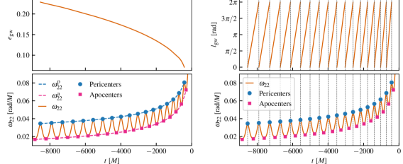
In Eq. (4), the pericenter and apocenter times can be chosen to correspond to local maxima and minima, respectively, in $\omega_{22}(t)$. This procedure is illustrated in the bottom-left panel of Fig. 1. It is not guaranteed that the local extrema of $\omega_{22}$ coincide with the local extrema of $\Omega_{\text{orb}}$. Instead, we can define the local extrema of $\omega_{22}$ to correspond to pericenters and apocenters. Other choices for assigning pericenter/apocenter times and their impact on the eccentricity will be discussed in Sec. III.

Because of its simplicity and gauge-independent nature, Eq. (4) has been applied to parameterize eccentric waveforms as well as GW data analysis Ramos-Buades et al. (2020a); Islam et al. (2021); Ramos-Buades et al. (2022a); Bonino et al. (2023). However, as shown in Ref. Ramos-Buades et al. (2022b), this definition of eccentricity does not have the correct Newtonian limit at large separations. In particular, in the small eccentricity limit at Newtonian order, one obtains Ramos-Buades et al. (2022b):

$$\lim_{e_{t}\rightarrow 0}e^{\text{0PN}}_{\omega_{22}}=\frac{3}{4}e_{t}+\mathcal{O}(e_{t}^{3}),$$ (7)

where $e_{t}$ is the temporal eccentricity used in PN theory, which matches the Newtonian eccentricity at Newtonian order Blanchet (2014).

This discrepancy can be resolved by using the following transformation Ramos-Buades et al. (2022b)

$$e_{\text{gw}}=\cos(\Psi/3)-\sqrt{3}\,\sin(\Psi/3),$$ (8)

where

$$\Psi=\arctan\left(\frac{1-e_{\omega_{22}}^{2}}{2\,e_{\omega_{22}}}\right).$$ (9)

Eq. (8) has the correct Newtonian limit over the full range of eccentricities Ramos-Buades et al. (2022b), and we adopt this definition in this work. As we will show in Sec. IV.1, $e_{\text{gw}}$ also approximately matches the geodesic eccentricity in the extreme mass ratio limit, while $e_{\omega_{22}}$ does not.

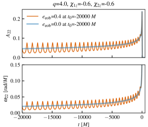
The top-left panel of Fig. 1 shows an example evaluation of $e_{\text{gw}}(t)$ for an NR simulation produced using the Spectral Einstein Code Boyle et al. (2011); SXS Collaboration (SpEC), developed by the Simulating eXtreme Spacetimes (SXS) collaboration SXS . As expected, $e_{\text{gw}}$ monotonically decreases as the binary approaches the merger ($t=0$). However, while the waveform itself covers the full range of times shown, $e_{\text{gw}}(t)$ does not. This is because $e_{\text{gw}}(t)$ depends on the $\omega^{\text{p}}_{22}(t)$ and $\omega^{\text{a}}_{22}(t)$ interpolants in Eq. (4), which do not span the full time range, as shown in the bottom-left panel of Fig. 1. $\omega^{\text{p}}_{22}(t)$ is only defined between the first and last available pericenters, and $\omega^{\text{a}}_{22}(t)$ is only defined between the first and last available apocenters. Therefore, the first available time for $e_{\text{gw}}(t)$ is the maximum of the times of the first pericenter and first apocenter. Similarly, the last available time for $e_{\text{gw}}(t)$ is the minimum of the times of the last pericenter and last apocenter.

Furthermore, we find that $e_{\text{gw}}(t)$ near the merger can become nonmonotonic, which is not surprising as it becomes hard to define an orbit in this regime. To avoid this nonmonotonic behavior, we discard the last two orbits of the waveform before computing $e_{\text{gw}}$. As a result, the last available time for $e_{\text{gw}}$ is the minimum of the times of the last pericenter and last apocenter in the remaining waveform, which falls at about two orbits before the peak amplitude. In addition, to successfully build the $\omega^{\text{p}}_{22}(t)$ and $\omega^{\text{a}}_{22}(t)$ interpolants in Eq. (4), we require at least two orbits in the remaining waveform. Therefore, the full waveform should include at least $\mathchar 21016\relax\,4-5$ orbits to reliably compute $e_{\text{gw}}$.

II.3.1 Extending to spin-precessing and frequency-domain waveforms

Eqs. (4) and (8) use only the $(2,2)$ mode as it is the dominant mode of radiation Varma and Ajith (2017); Varma et al. (2014); Capano et al. (2014), at least for binaries without spin-precession in which the direction of the orbital angular momentum is fixed (taken to be along $\hat{z}$ by convention). On the other hand, for spin-precessing binaries, the orbital angular momentum direction varies, and the power of the $(2,2)$ mode leaks into the other $\ell=2$ modes, meaning that there need not be a single dominant mode of radiation. For this reason, we restrict ourselves to binaries without spin-precession in this work. We expect that our method can be generalized to spin-precessing binaries by using $\mathpzc{h}_{22}$ in the coprecessing frame Boyle et al. (2011); Schmidt et al. (2011); O’Shaughnessy et al. (2011), which is a non-inertial frame that tracks the binary’s spin-precession so that $\hat{z}$ is always along the instantaneous orbital angular momentum. Alternatively, one could replace $\omega_{22}$ in Eq. (4) with a frame-independent angular velocity Boyle (2013) that incorporates information from all available waveform modes.

We also restrict ourselves to time-domain waveforms in this work. One main difficulty for frequency-domain waveforms Moore et al. (2018); Moore and Yunes (2019) is the identification of the frequencies at which pericenters and apocenters occur. This is complicated by the fact that even for the $(2,2)$ mode, eccentricity excites higher harmonics that make it difficult to identify local extrema in the frequency domain (see e.g. Fig. 3 of Ref. Moore et al. (2018)). Alternatively, one could simply apply an inverse Fourier transform to first convert the frequency-domain waveform to time-domain, although this can be computationally expensive for long signals.

II.4 Defining mean anomaly using the waveform

To fully describe an eccentric orbit at a given reference frequency, two parameters are required: eccentricity and mean anomaly Blanchet (2014); Schmidt et al. (2017); Islam et al. (2021), which is the fraction of the orbital period (expressed as an angle) that has elapsed since the last pericenter passage. Similar to $e_{\text{gw}}$, we seek a definition of mean anomaly that depends only on the waveform at future null-infinity. This can be achieved by generalizing the Newtonian definition of mean anomaly to Schmidt et al. (2017); Ramos-Buades et al. (2020a, 2022b); Islam et al. (2021)

$$l_{\text{gw}}(t)=2\pi\,\frac{t-t^{\text{p}}_{i}}{t^{\text{p}}_{i+1}-t^{\text{p}}_{i}},$$ (10)

defined over the interval $t^{\text{p}}_{i}\leq t<t^{\text{p}}_{i+1}$ between any two consecutive pericenter passages $t^{\text{p}}_{i}$ and $t^{\text{p}}_{i+1}$. $l_{\text{gw}}$ grows linearly in time over the range $[0,2\pi)$ between $t=t^{\text{p}}_{i}$ and $t=t^{\text{p}}_{i+1}$. In Newtonian gravity, the period of the orbit $T=t^{\text{p}}_{i+1}-t^{\text{p}}_{i}$ remains constant, while in general relativity, radiation reaction cause $T$ to decrease over time, making $l_{\text{gw}}(t)$ a stepwise linear function whose slope increases as as the binary approaches the merger. As the times corresponding to pericenter passages are already determined when calculating $e_{\text{gw}}$, computing $l_{\text{gw}}$ is straightforward. This procedure is illustrated in the right panel of Fig. 1.

We stress that the mean anomaly cannot be absorbed into a time or phase shift Islam et al. (2021), and is instead an intrinsic property of the binary like the component masses, spins and $e_{\text{gw}}$. This can be seen from the bottom-right panel of Fig. 1, showing $\omega_{22}(t)$. Consider the first pericenter occurring at $t\simeq-8500M$, for which $l_{\text{gw}}=0$. First, because $\omega_{22}$ is insensitive to phase shifts, one cannot apply a phase shift to change the mean anomaly at $t\simeq-8500M$ away from $l_{\text{gw}}=0$. Similarly, one cannot apply a time shift so that the mean anomaly at $t\simeq-8500M$ is changed, without simultaneously also changing the frequency at that time (because the time shift also applies to $\omega_{22}(t)$). In other words, to change the mean anomaly at a fixed time before the merger, one also needs to change the frequency at a fixed time before the merger, which results in a different physical system. Ignoring mean anomaly in waveform models and/or parameter estimation can result in systematic biases in the recovered source parameters Islam et al. (2021); Clarke et al. (2022); Ramos-Buades et al. (2023).

II.5 Generalizing the reference frequency $f_{\text{ref}}$

Binary parameters like the component spin directions, and orientation with respect to the observer, as well as eccentricity and mean anomaly, can vary during a binary evolution. Therefore, when measuring binary parameters from a GW signal, one needs to specify at which point of the evolution the measurement should be done. This is typically chosen to be the point at which the GW frequency crosses a reference frequency $f_{\text{ref}}$, with a typical choice of $f_{\text{ref}}=20$Hz Abbott et al. (2021a) as that is approximately where the sensitivity band of current ground-based detectors begins.

Figure 2: Different methods to construct a monotonically increasing frequency to replace $\omega_{22}(t)$, in order to set the reference frequency $f_{\text{ref}}$ for eccentric binaries. We consider two different approaches: (i) $\omega^{\text{mean}}_{22}(t)$, the mean of $\omega^{\text{p}}_{22}(t)$ and $\omega^{\text{a}}_{22}(t)$, and (ii) $\langle\omega_{22}\rangle(t)$, an interpolant through the orbit averaged $\omega_{22}$ (Eq. (12)). We show SEOBNRv4EHM waveforms with three different eccentricities; the binary parameters are given in the figure text. While the two approaches agree for small eccentricities, they deviate significantly at large eccentricities. We adopt $\langle\omega_{22}\rangle(t)$ as it captures the correct frequency scale in an orbit-averaged sense (Sec. II.5).

For quasicircular binaries without spin-precession, the GW frequency increases monotonically, and $f_{\text{ref}}$ can be uniquely associated with a reference time $t_{\text{ref}}$. For spin-precessing, quasicircular binaries, while $\omega_{22}$ in the inertial frame can be nonmonotonic, one can use the frequency computed in the coprecessing frame, which is always monotonically increasing Boyle et al. (2011); Varma et al. (2019a). Unfortunately, no such frame exists for eccentric binaries, and $\omega_{22}$ becomes nonmonotonic if eccentricity is sufficiently high (see Fig. 1).

Therefore, unique specification of a reference point via a frequency $f_{\text{ref}}$ requires a generalization of $\omega_{22}$ that is monotonically increasing, and approaches $\omega_{22}$ in the quasicircular limit. In the following we discuss two different ways to accomplish this and point out why the second is superior.

II.5.1 Mean of $\omega^{\text{p}}_{22}(t)$ and $\omega^{\text{a}}_{22}(t)$

A simple method to compute a monotonically increasing frequency for eccentric binaries is to take the mean of the interpolants through the frequencies at pericenters ($\omega^{\text{p}}_{22}(t)$) and apocenters ($\omega^{\text{a}}_{22}(t)$), both of which are monotonically increasing functions of time:

$$\omega^{\text{mean}}_{22}(t)=\frac{1}{2}\left[\omega^{\text{p}}_{22}(t)+\omega^{\text{a}}_{22}(t)\right],$$ (11)

with the reference time defined as $\omega^{\text{mean}}_{22}(t_{\text{ref}})=2\pi f_{\text{ref}}$.

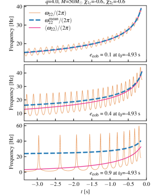
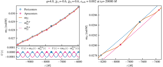
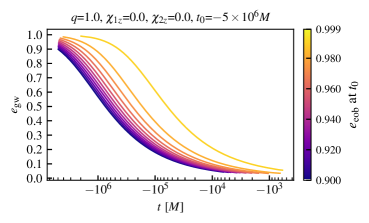
As $\omega^{\text{p}}_{22}(t)$ and $\omega^{\text{a}}_{22}(t)$ are already constructed when computing $e_{\text{gw}}$, there is no additional computational cost. Furthermore, as $\omega^{\text{p}}_{22}$ and $\omega^{\text{a}}_{22}$ approach $\omega_{22}$ in the quasicircular limit, so does $\omega^{\text{mean}}_{22}$. This method was used to set the reference frequency in Ref. Bonino et al. (2023). Figure 2 shows examples of $\omega^{\text{mean}}_{22}(t)$ for waveforms produced using the SEOBNRv4EHM Ramos-Buades et al. (2022a) eccentric EOB model, for three different values of the model’s internal eccentricity parameter $e_{\text{eob}}$, defined at a time $t_{0}=-4.93$ s before the peak amplitude.

II.5.2 Orbit averaged $\omega_{22}$

Alternatively, one can use the orbit average of $\omega_{22}$ in fixing the reference point. Between any two consecutive pericenters $t^{\text{p}}_{i}$ and $t^{\text{p}}_{i+1}$ we define

$$\langle\omega_{22}\rangle_{i}^{\text{p}} =\frac{1}{t^{\text{p}}_{i+1}-t^{\text{p}}_{i}}\,\int_{t^{\text{p}}_{i}}^{t^{\text{p}}_{i+1}}\omega_{22}(t)\,\mathrm{d}t$$

$$=\frac{\phi_{22}(t^{\text{p}}_{i+1})-\phi_{22}(t^{\text{p}}_{i})}{t^{\text{p}}_{i+1}-t^{\text{p}}_{i}},$$ (12)

and associate $\langle\omega_{22}\rangle_{i}^{\text{p}}$ with the midpoint between $t^{\text{p}}_{i}$ and $t^{\text{p}}_{i+1}$:

$$\langle t\rangle^{\text{p}}_{i}=\frac{1}{2}\left(t^{\text{p}}_{i}+t^{\text{p}}_{i+1}\right).$$ (13)

Applying this procedure to all consecutive pairs of pericenter times, we obtain the set $\big{\{}\,\left(\langle t\rangle^{\text{p}}_{i},\langle\omega_{22}\rangle_{i}^{\text{p}}\right)\,\big{\}}$. Similarly, using all consecutive pairs of apocenter times $t^{\text{a}}_{i}$ and $t^{\text{a}}_{i+1}$, we obtain the set $\left\{\,\big{(}\langle t\rangle^{\text{a}}_{i},\langle\omega_{22}\rangle_{i}^{\text{a}}\big{)}\,\right\}$. Taking the union of these two datasets, we build a cubic spline interpolant in time to obtain $\langle\omega_{22}\rangle(t)$.

The resulting orbit averaged frequency $\langle\omega_{22}\rangle(t)$ is also monotonically increasing and reduces to $\omega_{22}(t)$ in the quasicircular limit. The reference time associated with a reference frequency is now determined via

$$\langle\omega_{22}\rangle(t_{\text{ref}})=2\pi f_{\text{ref}}.$$ (14)

This method was used in Refs. Ramos-Buades et al. (2023, 2022b). Compared to $\omega^{\text{mean}}_{22}(t)$, $\langle\omega_{22}\rangle(t)$ has the added costs of computing orbit averages and constructing a new interpolant. The orbit averages are very cheap to compute as they can be written in terms of phase differences (Eq. (12)). The cost of the interpolant scales with the number of orbits but it is generally also cheap to construct.

Figure 2 also shows $\langle\omega_{22}\rangle(t)$ for the same SEOBNRv4EHM waveforms. While $\omega^{\text{mean}}_{22}(t)$ and $\langle\omega_{22}\rangle(t)$ agree at small eccentricities, they deviate significantly at large eccentricities. Unlike $\omega^{\text{mean}}_{22}(t)$, $\langle\omega_{22}\rangle(t)$ has the additional property, albeit only in an orbit-averaged sense, that at the time $t_{\text{ref}}$ where $\langle\omega_{22}\rangle(t_{\text{ref}})=2\pi f_{\text{ref}}$, one GW cycle occurs over a time scale of $1/f_{\text{ref}}$. This also explains why for the high eccentricity case in Fig. 2 (bottom panel), $\langle\omega_{22}\rangle$ follows the general trend of $\omega_{22}$ more closely than $\omega^{\text{mean}}_{22}$. For these reasons, we will adopt $\langle\omega_{22}\rangle$ and Eq. (14) in the rest of the paper.

II.6 Selecting a good reference point

Given a reference frequency $f_{\text{ref}}$, Sec. II.5 describes how that can be used to pick a reference time, $t_{\text{ref}}$, in the binary’s evolution. Another important choice is what frequency to use for $f_{\text{ref}}$. Most current analyses for ground-based detectors use $f_{\text{ref}}=20$ Hz Abbott et al. (2021a), but we argue that this may not be suitable for eccentric binaries. Setting $f_{\text{ref}}=20$ Hz means that the reference time is chosen to be the point where the observed GW frequency (or its orbit average) at the detector crosses 20 Hz. However, the observed GW signals are redshifted because of cosmological expansion, and the observed GW frequency depends on the distance between the source and detector. Two identical binaries placed at different distances would therefore reach an observed frequency of 20 Hz at different points in their evolution. Because the eccentricity varies during the evolution, the measured eccentricities for these binaries will be different when they reach $f_{\text{ref}}=20$ Hz at the detector! This is particularly problematic for applications like constraining the astrophysical distribution of eccentricities of GW sources, as the same source can be mistaken to have two different eccentricities.

All binary parameters that vary during a binary’s evolution, like spin directions, could be prone to this problem. However, because spin tilts vary over spin-precession time scales spanning many orbits, this has not been a significant issue so far when constraining the astrophysical spin distribution Abbott et al. (2023a), with the exception of Ref. Varma et al. (2022b) where this effect was found to be important when modeling the full 6D spin distribution. Eccentricity, on the other hand, can change rapidly on an orbital time scale, especially in the late stages near the merger (see Fig. 1).

One way to avoid this problem is to use the GW frequency defined in the source frame instead of the detector frame. However, this requires assuming a cosmological model to compute the redshift between the two frames. This can be problematic for applications like independently extracting cosmological parameters like the Hubble parameter from GW signals Abbott et al. (2023b). Alternatively, one can use a dimensionless reference frequency $Mf_{\text{ref}}$ or time $t_{\text{ref}}/M$ as proposed by Ref. Varma et al. (2022a), where $M$ is the total mass in the detector frame. Both of these choices have the benefit of not depending on the distance to the source as the total mass measured in the detector frame is also redshifted and exactly cancels out the redshift of $f_{\text{ref}}$ and $t_{\text{ref}}$. Ref. Varma et al. (2022a) proposed reference points of $t_{\text{ref}}/M=-100$ (where $t=0$ is at the peak of the GW amplitude) and $Mf_{\text{ref}}=6^{-3/2}$ (the Schwarzschild inner-most-circular-orbit (ISCO) frequency), as these always occur close to the merger for comparable mass binaries, and certain spin parameters like the orbital-plane spin angles are best measured near the merger. For measuring eccentricity, an earlier dimensionless time or frequency may be more appropriate, as eccentricity can be radiated away before the binary approaches merger.

A more straightforward approach could be to set the reference point at a fixed number of orbits before a fixed dimensionless time ($t_{\text{ref}}/M$) or dimensionless orbit-averaged frequency ($M\langle\omega_{22}\rangle$). Here, we define one orbit as the period between two pericenter passages, as measured from the waveform. As the number of orbits defined with respect to a dimensionless time/frequency is also unaffected by the redshift, this serves the same purpose as a dimensionless time/frequency. The number of orbits also scales more naturally to EMRI systems, while dimensionless time/frequency may not. A similar approach was recently adopted by Ref. Romero-Shaw et al. (2023).

Another advantage of using a fixed number of orbits before a dimensionless time/frequency is that by using pericenters to define the number of orbits, we can always measure eccentricity at a fixed mean anomaly of $l_{\text{gw}}=0$. This can make it simpler to report posteriors for eccentric GW signals by reducing the dimensionality by one. Similarly, this can make it easier to connect GW observations to astrophysical predictions for GW populations, as the predictions would just need to be made at a single mean anomaly value. However, we stress that mean anomaly would still need to be included as a parameter in waveform models and parameter estimation, and it is only when computing the eccentricity from the waveform predictions in postprocessing that this simplification occurs.

To summarize, while the most appropriate choice will need to be determined by analyzing eccentric GW signals in a manner similar to Ref. Varma et al. (2022a), we propose that the reference point be chosen to be a fixed number of orbits (e.g. 10) before a fixed dimensionless time (e.g. $t_{\text{ref}}/M=-100$) or a fixed dimensionless orbit-averaged frequency (e.g. $M\langle\omega_{22}\rangle=2\pi\,6^{-3/2}$, the Schwarzschild ISCO frequency). While not all GW signals will enter the detector frequency band with $\sim 10$ orbits to go before the merger, this can be achieved by always generating GW templates with at least 10 orbits when analyzing the GW signals. One important question that remains is whether using a reference point that falls outside the detector band leads to systematic biases or complications during parameter estimation. We expect that as long as the number of orbits by which the reference point falls outside the band is small, such effects should be small, but we leave this investigation to future work.

II.7 Truncating eccentric time domain waveforms

GW detectors are most sensitive over certain frequency bands ($\sim 20$ Hz to $\sim 10^{3}$ Hz for LIGO-Virgo), and waveform predictions need to include all physical GW frequencies present in this region. For frequency domain waveform models this is achieved by evaluating the model starting at initial frequency $f_{\text{low}}=20$ Hz. On the other hand, time-domain waveform models need to be evaluated starting at an initial time $t_{\text{low}}$, chosen so that the GW signal at earlier times does not contain any frequencies above $f_{\text{low}}$. In other words, the part of the time domain waveform that is not included ($t<t_{\text{low}}$) does not contribute to the GW signal in the detector frequency band.

Figure 3: How to truncate time domain eccentric waveforms while retaining all frequencies above $f_{\text{low}}=20$ Hz. The orange, blue and pink curves show different sections of $\omega_{22}(t)$ for an eccentric SEOBNRv4EHM waveform (with binary parameters shown in the title). If we discard all times below the point where the orbit-averaged frequency $\langle f_{22}\rangle\equiv\langle\omega_{22}\rangle/(2\pi)$ (pink dashed curve) crosses $f_{\text{low}}=20$ Hz, only the pink section is retained and the blue section is discarded even though it contains some frequencies above $20$ Hz. On the other hand, using $f_{22}^{\text{p}}\equiv\omega^{\text{p}}_{22}/(2\pi)$ (blue dashed curve) to pick this time ensures that the discarded region (orange) contains no frequencies above $20$ Hz.

For quasicircular waveform models with only the $(2,2)$ mode, $t_{\text{low}}$ can be chosen to be the time when

$$\omega_{22}(t_{\text{low}})=2\pi\,f_{\text{low}}.$$ (15)

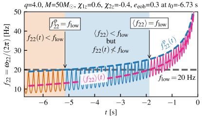
Because $\omega_{22}(t)$ is a monotonically increasing function for quasicircular binaries, frequencies $>f_{\text{low}}$ only occur at times $>t_{\text{low}}$. This is no longer the case for eccentric binaries as $\omega_{22}(t)$ can be nonmonotonic. An example is shown in Fig. 3, where we see that $\omega_{22}(t)/(2\pi)$ crosses $f_{\text{low}}=20$ Hz at several different times. One could choose the earliest of these crossings as $t_{\text{low}}$, but this only works if the original waveform is long enough to include all such crossings. If the original waveform only includes a subset of the crossings, this approach cannot guarantee that the discarded waveform only contains frequencies $<f_{\text{low}}$. To ensure all frequencies above $f_{\text{low}}$ are included, we need to generalize Eq. (15) to eccentric binaries.

A seemingly natural choice is to replace $\omega_{22}(t)$ in Eq. (15) with the monotonically increasing $\langle\omega_{22}\rangle(t)$ from Eq. (12):

$$\langle\omega_{22}\rangle(t_{\text{low}})=2\pi\,f_{\text{low}},$$ (16)

The pink dashed line in Fig. 3 shows $\langle\omega_{22}\rangle/(2\pi)$, and the frequencies retained when setting $t_{\text{low}}$ using Eq. (16) are also marked in pink. However, in this approach the section colored in blue is discarded, even though it still includes some frequencies above $f_{\text{low}}=20$ Hz.

Instead, we propose that $t_{\text{low}}$ should be set using the interpolant through pericenter frequencies, $\omega^{\text{p}}_{22}(t)$, which is already constructed when evaluating Eqs. (4) and (8).

$$\omega^{\text{p}}_{22}(t_{\text{low}})=2\pi\,f_{\text{low}}.$$ (17)

Because $\omega^{\text{p}}_{22}(t)$ represents the upper envelope of $\omega_{22}(t)$, this approach guarantees that the discarded waveform ($t<t_{\text{low}}$) does not contain any frequencies $>f_{\text{low}}$. This is demonstrated in Fig. 3, where we see that the blue section is included if Eq. (17) is used to set $t_{\text{low}}$.

So far, we only considered the $(2,2)$ mode when determining $t_{\text{low}}$. The frequency of the $(\ell,m)$ waveform mode (Eq. (1)) can be approximated during the inspiral as $\omega_{\ell m}(t)\sim(m/2)\leavevmode\nobreak\ \omega_{22}(t)$ Blanchet (2014). Therefore, for models containing higher modes, Eq. (17) should be replaced with:

$$\omega^{\text{p}}_{22}(t_{\text{low}})=\left(\frac{2}{m_{\text{max}}}\right)\,2\pi\,f_{\text{low}},$$ (18)

where $m_{\text{max}}$ is the largest $m$ among all included modes.

II.8 Summary

Our procedure to compute the eccentricity and mean anomaly from the waveform can be summarized as follows:

1. Find the times corresponding to the pericenters and apocenters, which we denote as $\{t^{\text{p}}_{i}\}$ and $\{t^{\text{a}}_{i}\}$, respectively. In the example in Fig. 1, $\{t^{\text{p}}_{i}\}$ and $\{t^{\text{a}}_{i}\}$ are identified as the local maxima and minima, respectively, of $\omega_{22}$, but other methods for locating these times will be discussed in Sec. III.

2. Evaluate $\omega_{22}(t)$ at $\{t^{\text{p}}_{i}\}$ and $\{t^{\text{a}}_{i}\}$ to get the frequencies at pericenters and apocenters and construct interpolants in time, $\omega^{\text{p}}_{22}(t)$ and $\omega^{\text{a}}_{22}(t)$, using these data. We use cubic splines for interpolation.

3. Obtain $e_{\omega_{22}}(t)$ using $\omega^{\text{p}}_{22}(t)$ and $\omega^{\text{a}}_{22}(t)$ in Eq. (4). Finally, apply the transformation in Eq. (8) to obtain the eccentricity $e_{\text{gw}}(t)$.

4. Use the pericenter times $\{t^{\text{p}}_{i}\}$ in Eq. (10) to compute the mean anomaly $l_{\text{gw}}(t)$.

5. To get the eccentricity and mean anomaly at a reference frequency $f_{\text{ref}}$, first use the orbit averaged frequency $\langle\omega_{22}\rangle(t)$ (Eq. (12)) to get the corresponding $t_{\text{ref}}$. However, instead of using a fixed $f_{\text{ref}}$ in Hz, a fixed dimensionless frequency or time, or a fixed number of orbits before a dimensionless frequency/time might be a better choice for eccentric binaries (Sec. II.6).

6. Use $\omega^{\text{p}}_{22}(t)$ (Eq. (18)) to truncate time-domain signals at a given start frequency $f_{\text{low}}$ so that the discarded waveform does not contain any frequencies above $f_{\text{low}}$.

III Methods to locate pericenters and apocenters

In Sec. II and Fig. 1, the pericenter and apocenter times are taken to correspond to local extrema in $\omega_{22}(t)$. Identifying these times is a crucial step in our definitions of eccentricity and mean anomaly, as well as the generalizations of $f_{\text{ref}}$ and $f_{\text{low}}$. In this section, we explore several different alternatives for identifying the pericenter/apocenter times and their benefits and drawbacks. Instead of $\omega_{22}(t)$, these methods set extrema in various other waveform quantities (like the amplitude) as the pericenter/apocenter times. Therefore, the pericenter/apocenter times can depend on the method used, and each of these alternatives should be viewed as a new definition of eccentricity and mean anomaly. However, all of these methods satisfy the criteria listed in Sec. II for a good definition of eccentricity, and as we will show in Sec. IV the differences between the different methods are generally small. We denote the waveform quantity whose extrema are used as $U(t)$. Given $U(t)$, we use the find_peaks routine within SciPy Virtanen et al. (2020) to locate the extrema.

III.1 Frequency and amplitude

The most straightforward choice for $U(t)$ is

$$U(t)=\omega_{22}(t),$$ (19)

as considered in Fig. 1. The local maxima in $U(t)$ are identified as the pericenters while the local minima are identified as apocenters. We refer to this method as the Frequency method.

Because $\omega_{22}(t)$ relies on a time derivative – see Eq. (6) – it can be noisy in some cases, especially for NR waveforms. Such noise can lead to spurious extrema in $\omega_{22}(t)$ that can be mistaken for pericenters/apocenters. Such problems can be avoided by locating the extrema of the amplitude of the $(2,2)$ mode, i.e.

$$U(t)=A_{22}(t).$$ (20)

We refer to this method as the Amplitude method and recommended it over the Frequency method.

The simplicity of the Frequency and Amplitude methods comes with the drawback that these methods fail for small eccentricities, as illustrated in Fig. 4. The top two rows show $\omega_{22}$ and $A_{22}$ for an eccentric SEOBNRv4EHM Ramos-Buades et al. (2022a) waveform. While local extrema can be found at early times, as eccentricity is radiated away, the prominence of the extrema decreases until local extrema cease to exist. The onset of this breakdown is signaled by the pericenters and apocenters converging towards each other, as seen in the figure insets. This occurs because at small eccentricity, the secular growth in $\omega_{22}$ and $A_{22}$ dominates the modulations due to eccentricity. We find that for eccentricities $e_{\text{gw}}\lesssim 10^{-2}\ldots 10^{-3}$ (see Sec. IV), the Frequency and Amplitude methods can fail to measure the eccentricity. This breakdown point can be approximately predicted by the following order-of-magnitude estimate.

Figure 4: Limitations of the Amplitude and Frequency methods in identifying pericenters (blue circles) and apocenters (pink squares) for a low eccentricity waveform. These methods (top two rows) detect only the first few pericenters/apocenters and fail once sufficient eccentricity is radiated away. On the other hand, the ResidualAmplitude and ResidualFrequency methods (bottom two rows) can detect all of the pericenters/apocenters present. The waveform is generated using SEOBNRv4EHM and the binary parameters are given in the title.

III.1.1 Estimating the breakdown point of the Frequency method

The inspiral rate of a binary in quasicircular orbit at Newtonian order is given by (e.g. Blanchet (2014))

$$\frac{\mathrm{d}\omega_{22}^{\rm circ}}{\mathrm{d}t}=\frac{192}{5}\nu\frac{1}{M^{2}}\left(\frac{M\omega_{22}^{\text{circ}}}{2}\right)^{11/3},$$ (21)

where $\nu=q/(1+q)^{2}$ is the symmetric mass ratio.

For small eccentricities, eccentricity induces an oscillatory component to the frequency,

$$\omega_{22}(t)\approx\omega_{22}^{\text{circ}}(t)+A\sin(\omega_{r}t),$$ (22)

where $\omega_{r}$ denotes the radial oscillation frequency. The amplitude $A$ of the oscillations can be related to eccentricity by substituting into Eq. (4) and expanding to first order in $A$, yielding $A=2e_{\omega_{22}}\,\omega_{22}^{\text{circ}}$. For a given short time interval, we take $A$ to be constant.

Extrema in $\omega_{22}(t)$ correspond to zeros of the time derivative

$$\frac{\mathrm{d}\omega_{22}}{\mathrm{d}t}\approx\frac{\mathrm{d}\omega_{22}^{\rm circ}}{\mathrm{d}t}+A\omega_{r}\cos(\omega_{r}t).$$ (23)

Such zeros exist only if the oscillatory component dominates over the inspiral part, $A\omega_{r}\gtrsim\mathrm{d}\omega_{22}^{\rm circ}/\mathrm{d}t$, i.e. for sufficiently large eccentricities:

$$e_{\omega_{22}}\gtrsim\frac{48}{5}\nu\left(\frac{M\omega_{22}}{2}\right)^{5/3}\frac{\omega_{22}}{2\omega_{r}}.$$ (24)

Here we have dropped the subscript “circ”, as $\omega_{22}^{\text{circ}}\approx\omega_{22}$ at leading order in the assumed small eccentricity. Neglecting pericenter advance, i.e. setting $\omega_{22}/(2\omega_{r})=1$, and noting that for small eccentricity, $e_{\omega_{22}}\approx(3/4)\,e_{\text{gw}}$ (Eq. 7), we find that local extrema in $\omega_{22}(t)$ are only present if

$$e_{\text{gw}}\gtrsim\frac{192}{15}\nu\left(\frac{M\omega_{22}}{2}\right)^{5/3}.$$ (25)

The systems considered in this paper have $\omega_{22}\sim 0.02/M\ldots 0.1/M$ (e.g. Figs. 1 or 4), so that for comparable mass binaries, Eq. (25) predicts a breakdown of the Frequency method for $e_{\text{gw}}\sim 10^{-3}\ldots 10^{-2}$.

This motivates us to consider alternative methods to detect local extrema that also work for small eccentricities. In the following, we will consider different methods that first subtract the secular growth in $\omega_{22}$ or $A_{22}$, and use the remainder as $U(t)$.

III.2 Residual frequency and residual amplitude

We begin with a simple extension of the Frequency method, which we refer to as the ResidualFrequency method:

$$U(t)=\Delta\omega_{22}(t)\equiv\omega_{22}(t)-\omega_{22}^{\text{circ}}(t),$$ (26)

and likewise the ResidualAmplitude method:

$$U(t)=\Delta A_{22}(t)\equiv A_{22}(t)-A_{22}^{\text{circ}}(t),$$ (27)

where $\omega_{22}^{\text{circ}}$ and $A_{22}^{\text{circ}}$ are the frequency and amplitude of the $(2,2)$ mode for a quasicircular counterpart of the eccentric binary. We define the quasicircular counterpart as a binary with the same component masses and spins, but with zero eccentricity. The time array of the quasicircular waveform is shifted so that its peak time coincides with that of the eccentric waveform. Once again, the local maxima in $U(t)$ are identified as the pericenters while the local minima are identified as apocenters.

Eqs. (26) and (27) are motivated by the observation Islam et al. (2021) that the quasicircular counterpart waveform captures the secular trend of the eccentric waveform, when the peak times of the waveforms are aligned. This is demonstrated for an example eccentric SEOBNRv4EHM waveform in Fig. 5. The quasicircular counterpart falls approximately at the midpoint between the peaks and troughs of amplitude and frequency of the eccentric waveform. We find this to be the case for the full range of eccentricities, and waveforms of all origins.

For an eccentric waveform model, the quasicircular counterpart can be easily generated by evaluating the model with eccentricity set to zero while keeping the other parameters fixed. For eccentric NR waveforms, such a quasicircular NR waveform may not exist and one can use a quasicircular waveform modelto generate the quasicircular counterpart. In this paper, we use the IMRPhenomT Estellés et al. (2022) quasicircular waveform model to generate quasicircular counterparts of NR waveforms and IMRPhenomT is currently set as the default choice in gw_eccentricity Shaikh et al. as it supports a wide range of values for the binary parameters. One can also use more accurate models like the NR surrogate model NRHybSur3dq8 Varma et al. (2019b) whenever the parameters fall within the regime of validity of the surrogate model. Similarly to how the different methods to locate extrema are part of the eccentricity definition, the choice of quasicircular model should also be considered to be a part of the definition. The impact of the choice of the quasicircular model on eccentricity is generally small and will be explored further in Sec. IV.4.

Figure 5: Comparison of the amplitude (top) and the frequency (bottom) of an eccentric SEOBNRv4EHM waveform to those of its quasicircular counterpart. The binary parameters are shown in the figure text. Both waveforms are aligned so that $t=0$ occurs at the peak of $A_{22}$. The quasicircular counterpart captures the secular growth in the amplitude and frequency of the eccentric waveform.

By first subtracting the secular growth in the eccentric waveform, the ResidualFrequency and ResidualAmplitude methods can detect local extrema even for small eccentricities. The bottom two rows of Fig. 4 show an example where these methods succeed while the Frequency and Amplitude methods fail. Once again, between ResidualFrequency and ResidualAmplitude, we recommend ResidualAmplitude as it is less prone to numerical noise for NR waveforms. While the ResidualFrequency and ResidualAmplitude are robust and straightforward to implement, their main drawback is that they require the evaluation of a quasicircular waveform, which increases the computational expense. We consider the next set of methods to model the secular trend without relying on additional waveform evaluations.

Figure 6: Illustration of the FrequencyFits method. Left: The blue circles indicate the $2N+1=7$ extrema through which the fitting function Eq. (30) passes. The lower panel shows the envelope-subtracted data from which the extrema $T_{\alpha}$ are determined. The solid blue circle indicates the central extremum, whose parameters are used for the eccentricity definition. The pink square and the pink dashed line show the analogous construction for the apocenter passages. Right: Enlargement of the region around the solid markers in the upper panel on the left. The waveform is generated using SEOBNRv4EHM, and the binary parameters are given in the title.

III.3 Frequency fits and amplitude fits

The ResidualAmplitude and ResidualFrequency methods described in Sec. III.2 have the disadvantage that they require a quasicircular reference waveform for subtraction. Such a reference waveform may not be available, or deviations in the reference waveform may lead to differences in the recovered eccentricity (see Sec. IV.4).

The FrequencyFits method avoids the need for a reference waveform by self-consistently fitting the envelopes $\omega^{\text{p}}_{22}(t)$ (for pericenters) and $\omega^{\text{a}}_{22}(t)$ (for apocenters) that appear in Fig. 1, an idea introduced in Lewis et al. Lewis et al. (2017). To simplify the explanation, we will first describe this method when applied to locate pericenters. The idea lies in considering a local stretch of data $\omega_{22}(t)$ for $t\in[t_{L},t_{R}]$, in which we identify the times $T_{\alpha}$ (labeled by $\alpha$) as local maxima of the envelope-subtracted frequency (Eq. (28)), while self-consistently constructing the envelope fit $\omega^{\text{fit},\text{p}}_{22}(t)$ through $\omega_{22}(t)$ evaluated at $T_{\alpha}$. The fit $\omega^{\text{fit},\text{p}}_{22}(t)$, the local maxima times $T_{\alpha}$, and the interval $[t_{L},t_{R}]$ are iteratively refined and the central $T_{\alpha}$ is identified as a pericenter time.

To make this idea precise, we start by choosing a time $\hat{t}$, which will roughly correspond to the middle of the fitting interval. We now seek to determine a fitting function $\omega^{\text{fit},\text{p}}_{22}(t)$ through the pericenter frequencies, valid in a time-interval $[t_{L},t_{R}]$ encompassing $\hat{t}$, as well as times $T_{\alpha}\in[t_{L},t_{R}]$, $\alpha=0,\ldots,2N$ (with $N=3$, as explained after Eq. (31)). These quantities are determined in a self-consistent manner such that the following conditions are all satisfied:

1. $T_{\alpha}$ are local maxima of the envelope-subtracted frequency $U(t)$ given by:

   $$U(t)=\omega_{22}(t)-\omega^{\text{fit},\text{p}}_{22}(t).$$ (28)

2. $\omega^{\text{fit},\text{p}}_{22}(t)$ is a fit through the $2N+1$ evaluations of $\omega_{22}(t)$ at times $T_{\alpha}$, i.e. $(T_{\alpha},\omega_{22}(T_{\alpha}))$ in the interval $[t_{L},t_{R}]$,

   $$\omega^{\text{fit},\text{p}}_{22}(T_{\alpha})\approx\omega_{22}(T_{\alpha}),\quad\alpha=0,\ldots,2N.$$ (29)

3. The time-interval $[t_{L},t_{R}]$ contains precisely $2N+1$ local maxima of $U(t)$ where the first $N$ are before $\hat{t}$, and the others after.

If these conditions are met, then the extremum in the middle, $(T_{N},\omega_{22}(T_{N}))$ will be identified as a pericenter passage, and included in the overall list of pericenters for the inspiral.

This procedure is illustrated in Fig. 6. The top panel shows $\omega_{22}(t)$ in orange, for a configuration with eccentricity so small that $\omega_{22}(t)$ does not have extrema. The locations of the identified local maxima $\big{(}T_{\alpha}$, $\omega_{22}(T_{\alpha})\big{)}$ are indicated by blue circles, with the middle one (corresponding to $T_{N}$) being filled. The lower panel shows the envelope subtracted function, whose maxima determine the $T_{\alpha}$.

In practice, the fitting function is chosen to have the functional form

$$\omega^{\text{fit},\text{p}}_{22}(t;\,A,\,n,\,t_{\rm merg})=A(t_{\rm merg}-t)^{n},$$ (30)

with fit-parameters $\{A,n,t_{\rm merg}\}$. The form of Eq. (30) is inspired by the leading order PN behavior of a quasicircular binary inspiral, which has the form of Eq. (30) with exponent $-3/8$ Blanchet (2014). In addition, Eq. (30) ensures monotonicity by construction. To reduce correlations between the parameters $A$ and $n$, the fitting function is reparameterized by $\{f_{0},f_{1},t_{\rm merg}\}$ where $f_{0}$ and $f_{1}$ represent the function value and first time-derivative at a time $t_{\rm mid}$,

$$f_{0}= A(t_{\rm merg}-t_{\rm mid})^{n},$$ (31a)

$$f_{1}= -nA(t_{\rm merg}-t_{\rm mid})^{n-1}=-n\frac{f_{0}}{t_{\rm merg}-t_{\rm mid}}.$$ (31b)

Equations (31) are readily inverted to yield

$$n= -\frac{f_{1}(t_{\rm merg}-t_{\rm mid})}{f_{0}},$$ (32a)

$$A= f_{0}(t_{\rm merg}-t_{\rm mid})^{-n}.$$ (32b)

The fit for $\{f_{0},f_{1},t_{\rm merg}\}$ is performed with the curve_fit routine of the SciPy Virtanen et al. (2020) library. Because there are three free parameters, at least three local maxima are needed to perform the fit; we choose $2N+1=7$ maxima for increased robustness. The concrete choice for $t_{\rm mid}$ is found to be not critical; we choose the time in the middle of the entire waveform to be analyzed.

To analyze an entire waveform, we proceed from the start of the waveform toward the merger. At the first, “cold” initialization at the start of the waveform, we choose $t_{L}$ to be the start of the waveform, $\hat{t}$ to be $N$ orbits later (as judged by the accumulated $\phi_{22}$), and $t_{R}$ to be $2N$ orbits later. We initialize a first guess for $\omega^{\text{fit},\text{p}}_{22}$ through a fit to $\omega_{22}(t)$ during the first 10 orbits of the waveform.

In order to satisfy the conditions 1 to 3 self-consistently, an iterative procedure is applied: local maxima of $U(t)$ are calculated using find_peaks, and the interval $[t_{L},t_{R}]$ is adjusted to achieve the desired number of extrema on either side of $\hat{t}$. Now an improved $\omega^{\text{fit},\text{p}}_{22}$ is computed by fitting to the extrema, Eq. (29), and the procedure is iterated until the changes in the extrema $T_{\alpha}$ and fitting parameters $\{f_{0},f_{1},T\}$ fall below a tolerance, typically $10^{-8}$. At the initial cold start, this typically takes 3-5 iterations.

We then shift the analysed region by one pericenter passage at a time, i.e. $\hat{t}\to\hat{t}=(T_{N}+T_{N+1})/2$, $t_{L}\to(T_{0}+T_{1})/2$, $t_{R}\to T_{2N}+1.5\,\!\times\!\,(T_{2N}-T_{0})/(2N)$, and repeat the iterative procedure to satisfy conditions 1 to 3, using the current $\omega^{\text{fit},\text{p}}_{22}$ as the initial guess. Because of the improved guess for $\omega^{\text{fit},\text{p}}_{22}$, each successive pericenter passage needs only 2–3 iterations to converge. We stop the procedure when $t_{L}$ reaches the end of the waveform, or when all three conditions can no longer be simultaneously satisfied. For instance, in rare cases, the iterative procedure settles into a limiting cycle, which switches between two different results for the interval $[t_{L},t_{R}]$, the extrema $T_{\alpha}$, and the fit $\omega^{\text{fit},\text{p}}_{22}$.

Equation (28) identifies local maxima of $\omega_{22}(t)-\omega^{\text{fit},\text{p}}_{22}(t)$, i.e. pericenter passages. To identify apocenter passages, we change the sign of the right-hand-side of Eq. (28), while keeping the remainder of the algorithm unchanged. The algorithm will then generate a fit to the apocenter points, $\omega^{\text{fit},\text{a}}_{22}$, as indicated in pink in Fig. 6.

The procedure outlined above also works if we fit the amplitude $A_{22}$ in place of $\omega_{22}$, since at leading post-Newtonian order, the amplitude also has the form of Eq. (30) with exponent $-1/4$ Blanchet (2014). We refer to the method of finding the pericenters/apocenters by fitting to $A_{22}$ as AmplitudeFits. Once again, FrequencyFits is more prone to numerical noise as it relies on $\omega_{22}$. Therefore, we recommend AmplitudeFits over FrequencyFits.

IV Robustness tests

In this section, we check the robustness of our eccentricity definition and the different methods to locate pericenters/apocenters by putting our implementation through various tests.

IV.1 The large mass ratio limit of $e_{\text{gw}}$

In Sec. I, we noted that one of the desired but not strictly required features of an ideal eccentricity definition is that in the limit of large mass ratio, it should approach the test particle eccentricity on a Kerr geodesic. The geodesic eccentricity $e_{\text{geo}}$ typically used for EMRI calculations Darwin (1959, 1961) is given by:

$$e_{\text{geo}}=\frac{r^{\text{a}}-r^{\text{p}}}{r^{\text{a}}+r^{\text{p}}},$$ (33)

where $r^{\text{p}}$ and $r^{\text{a}}$ are the pericenter and apocenter separations along the geodesic in Boyer–Lindquist coordinates. To test the test particle limit of $e_{\text{gw}}$, we compare $e_{\text{gw}}$ and $e_{\text{geo}}$ for an EMRI waveform with $q=\infty$ and nonspinning BHs, but with varying eccentricities in the range $e_{\text{geo}}\in[0,0.5]$. In the $q\to\infty$ limit, there is no orbital evolution and the waveform is that of a test particle following a geodesic. For our comparisons, we use the waveforms computed within this framework in Ref. Ramos-Buades et al. (2022b) using a frequency domain Teukolsky code. Because there is no orbital evolution these waveforms each have a constant value of eccentricity $e_{\text{geo}}$ and orbit averaged frequency $\langle\omega_{22}\rangle$.

Figure 7: Comparison of $e_{\text{gw}}$ and $e_{\omega_{22}}$ to the geodesic eccentricity $e_{\text{geo}}$ in the $q\to\infty$ limit, as a function of the orbit averaged frequency $\langle\omega_{22}\rangle$. In the left panel, the colors show the absolute difference between $e_{\text{geo}}$ and $e_{\text{gw}}$ measured using Eq. (8) with the Amplitude method. The right panel shows the same for $e_{\omega_{22}}$. $e_{\text{geo}}$ is closer to $e_{\text{gw}}$ than $e_{\omega_{22}}$ by about two orders of magnitude.

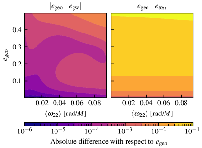
Figure 7 shows the differences $|e_{\text{geo}}-e_{\text{gw}}|$ and $|e_{\text{geo}}-e_{\omega_{22}}|$, evaluated at different values of $e_{\text{geo}}$ and $\langle\omega_{22}\rangle$. While $e_{\text{gw}}$ does not exactly match $e_{\text{geo}}$ in the test particle limit, the differences for $e_{\text{gw}}$ lie in the range $\sim[10^{-6},6\!\times\!10^{-3}]$, whereas the differences for $e_{\omega_{22}}$ lie in the range $\sim[5\!\times\!10^{-4},10^{-1}]$. Therefore, $e_{\text{gw}}$ is an improvement over $e_{\omega_{22}}$ in two ways: $e_{\text{gw}}$ has the correct Newtonian limit (as shown by Ref. Ramos-Buades et al. (2022a)) and is closer to $e_{\text{geo}}$ in the test particle limit, by about two orders of magnitude.

Figure 8: Demonstration of the measurement of eccentricity using the gw_eccentricity Shaikh et al. package for waveforms of different origins: PN, EOB, NR and EMRI. The binary parameters are indicated in the figure text. In each subplot, the lower panel shows the real part of $\mathpzc{h}_{22}$, and the upper panel shows the measured eccentricity. We consider three different methods for identifying the pericenters/apocenters: Amplitude, ResidualAmplitude and AmplitudeFits.

IV.2 Applicability for waveforms of different origins

Another criteria for the eccentricity definition identified in Sec. I that is desired but not strictly required is that it should be robust and applicable for waveforms of different origins, such as analytical PN waveforms Memmesheimer et al. (2004); Huerta et al. (2014); Tanay et al. (2016); Cho et al. (2022); Moore et al. (2018); Moore and Yunes (2019), numerical waveforms from NR Hinder et al. (2018); Boyle et al. (2019); Islam et al. (2021); Ramos-Buades et al. (2022b); Healy and Lousto (2022); Habib and Huerta (2019); Huerta et al. (2019); Hinder et al. (2018); Boyle et al. (2019); Ramos-Buades et al. (2022b); Healy and Lousto (2022); Habib and Huerta (2019); Huerta et al. (2019) simulations, semi-analytical EOB waveforms calibrated to NR Cao and Han (2017); Liu et al. (2020); Ramos-Buades et al. (2022a); Nagar et al. (2021), and EMRI Warburton et al. (2012); Osburn et al. (2016); van de Meent and Warburton (2018); Chua et al. (2021); Hughes et al. (2021); Katz et al. (2021); Lynch et al. (2022); Barack and Sago (2010); Akcay et al. (2013); Hopper and Evans (2013); Osburn et al. (2014); van de Meent and Shah (2015); Hopper et al. (2016); Forseth et al. (2016); van de Meent (2016, 2018); Munna et al. (2020); Munna and Evans (2020, 2022a, 2022b) waveforms obtained by solving the Teukolsky equation.

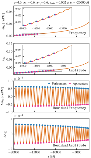
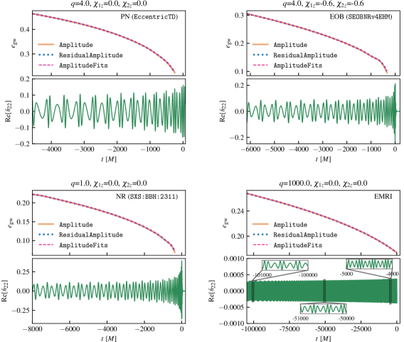
In Fig. 8 we show examples of our $e_{\text{gw}}$ implementation in gw_eccentricity Shaikh et al. applied to waveforms of four different origins: PN (EccentricTD Tanay et al. (2016)), EOB (SEOBNRv4EHM Ramos-Buades et al. (2022a)), NR (SpEC SXS Collaboration ; Islam et al. (2021)), and EMRI (Ref. Ramos-Buades et al. (2022b)). The binary parameters are arbitrarily chosen to cover a wider parameter space and are shown in the figure text. In each of the four subplots in Fig. 8, the lower panel shows the real part of $\mathpzc{h}_{22}$, and the upper panel shows the measured $e_{\text{gw}}$. We consider three different methods to locate the pericenters/apocenters Amplitude, ResidualAmplitude, and AmplitudeFits, and $e_{\text{gw}}$ is consistent between the three methods. For the ResidualAmplitude method, for the PN, EOB and EMRI cases, we use the same model evaluated at zero eccentricity for the quasicircular counterpart. For NR, we use the IMRPhenomT Estellés et al. (2022) model.

In addition to Fig. 8, we have tested our implementation in gw_eccentricity Shaikh et al. against eccentric SpEC NR waveforms from Refs. Islam et al. (2021); Ramos-Buades et al. (2022b). When testing against eccentric NR simulations from the RIT catalog RIT ; Healy and Lousto (2022), we are able to compute $e_{\text{gw}}$ whenever the waveform contains at least $\mathchar 21016\relax\,4-5$ orbits before the merger, for reasons explained in Sec. II.3. Finally, we have conducted extensive robustness tests using the SEOBNRv4EHM model in different regions of the parameter space, including converting $e_{\text{eob}}$ posterior samples to $e_{\text{gw}}$ samples in a postprocessing step after parameter estimation.

IV.3 Smoothness tests

Figure 9: $e_{\text{gw}}$ vs $e_{\text{eob}}$ at the initial time, for SEOBNRv4EHM waveforms with varying $e_{\text{eob}}$, but keeping the other binary parameters fixed (given in figure title). $e_{\text{eob}}$ is the model’s internal eccentricity, specified at $t_{0}=-20000M$. $e_{\text{gw}}$ is evaluated at its first available time, $\widehat{t}_{0}$. We consider three different methods for locating pericenters/apocenters: Amplitude, ResidualAmplitude, and AmplitudeFits. The Amplitude method breaks down for small eccentricities ($e_{\text{eob}}\lesssim 10^{-3}$), while the ResidualAmplitude and AmplitudeFits method follow the expected $e_{\text{gw}}=e_{\text{eob}}$ trend down to $e_{\text{eob}}=10^{-5}$.

In this section, we demonstrate that our implementation of $e_{\text{gw}}$ varies smoothly as a function of internal definitions of eccentricity used by waveform models. Specifically, we generate 50 waveforms using the SEOBNRv4EHM model Ramos-Buades et al. (2022a), with the model’s internal eccentricity parameter varying from $e_{\text{eob}}=10^{-7}$ to $e_{\text{eob}}=0.9$,  while keeping the other parameters fixed at $q=4$, and $\chi_{1z}=\chi_{2z}=-0.6$. The eccentricity $e_{\text{eob}}$ refers to the start of each waveform, which we choose to be at $t_{0}=-20000M$ before the peak waveform amplitude.  In addition to testing whether $e_{\text{gw}}$ varies smoothly, this test also demonstrates that our implementation in gw_eccentricity Shaikh et al. works over a wide range of eccentricities. Both of these features are important for applications like converting posterior samples for $e_{\text{eob}}$ to the standardized $e_{\text{gw}}$.

For simplicity, we restrict our consideration to the three preferred methods from Sec III, Amplitude, ResidualAmplitude and AmplitudeFits. The Frequency, ResidualFrequency and FrequencyFits methods perform similarly to Amplitude, ResidualAmplitude and AmplitudeFits methods, respectively, but can be prone to numerical noise.

IV.3.1 $e_{\text{gw}}$ vs $e_{\text{eob}}$ at initial time

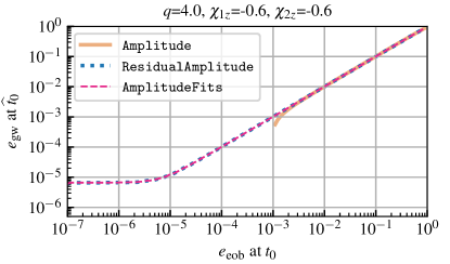
We first compare $e_{\text{eob}}$ (which is defined at $t_{0}=-20000M$) to $e_{\text{gw}}$ at its first available time (which we denote as $\widehat{t}_{0}$). As described in Sec. II.3, the first available time for $e_{\text{gw}}(t)$ is the maximum of the times of the first pericenter and first apocenter, as starting at this time, both $\omega^{\text{p}}_{22}(t)$ and $\omega^{\text{a}}_{22}(t)$ interpolants in Eq. (4) can be defined. For our dataset of SEOBNRv4EHM waveforms, this time varies from $\widehat{t}_{0}=-19250M$ for $e_{\text{eob}}=10^{-7}$ to $\widehat{t}_{0}=-15250M$ for $e_{\text{eob}}=0.9$. However because the difference between $\widehat{t}_{0}$ and $t_{0}$ is always within an orbit, and eccentricity does not change significantly over one orbit, comparing $e_{\text{gw}}$ at $\widehat{t}_{0}$ to $e_{\text{eob}}$ at $t_{0}$ is reasonable.  The ideal outcome for this test is that the eccentricity measured from the waveform $e_{\text{gw}}$ matches the model’s eccentricity definition $e_{\text{eob}}$.

Figure 9 shows how $e_{\text{gw}}$ at $\widehat{t}_{0}$ varies with $e_{\text{eob}}$ at $t_{0}$, for the Amplitude, ResidualAmplitude and AmplitudeFits methods. For sufficiently high eccentricities ($e_{\text{eob}}\gtrsim 5\!\times\!10^{-3}$), all three methods follow the expected trend of $e_{\text{gw}}=e_{\text{eob}}$. However, the Amplitude method starts to deviate from this trend for smaller eccentricities, before completely breaking down for $e_{\text{eob}}\lesssim 10^{-3}$. This is expected as local extrema do not exist in $A_{22}$ for such low eccentricities (see Sec. III).

Figure 10: $e_{\text{gw}}$ vs the internal definition of eccentricity, for waveforms of different origin, for equal-mass nonspinning binaries with varying eccentricity. For the NR waveforms (SpEC), we compute the internal eccentricity at $t_{0}=1500M$ after the start of the simulation, while for the rest we use $t_{0}=-20000M$ before peak waveform amplitude. In both cases, $\widehat{t}_{0}$ is the first available time for $e_{\text{gw}}(t)$. The inset shows the same but on a linear scale, and focuses on the $e_{\text{gw}}\leq 0.4$ region.

By contrast, the ResidualAmplitude and AmplitudeFits method follow the $e_{\text{gw}}=e_{\text{eob}}$ trend all the way down to $e_{\text{eob}}=10^{-5}$. For smaller $e_{\text{eob}}$, the SEOBNRv4EHM model itself ceases producing waveforms for which the modulations due to eccentricity decrease with decreasing $e_{\text{eob}}$. For most practical applications, this is not problematic for SEOBNRv4EHM as $e_{\text{eob}}=10^{-5}$ is very small. However, this exercise highlights how (in addition to testing our implementation) tests like this can help identify the limitations of eccentric waveform models.

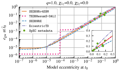
In this spirit, we repeat this test for several different eccentric waveform models in Fig. 10. For an equal-mass nonspinning binary, we show how $e_{\text{gw}}$ at $\widehat{t}_{0}$ varies with the internal definitions of eccentricity (defined at $t_{0}=-20000M$) used by the SEOBNRv4EHM Ramos-Buades et al. (2022a), TEOBResumS-DALI Nagar et al. (2018, 2021), SEOBNRE Cao and Han (2017); Liu et al. (2020), and EccentricTD Tanay et al. (2016) models. For simplicity, we only consider the ResidualAmplitude method, where the quasicircular counterpart is obtained by evaluating the same model at zero eccentricity.

Figure 10 also shows the dependence of $e_{\text{gw}}$ on the internal definition of eccentricity for a few eccentric equal-mass nonspinning NR simulations produced with the SpEC code Boyle et al. (2019); SXS Collaboration ; Islam et al. (2021) (with SXS IDs 2267, 2270, 2275, 2280, 2285, 2290, 2294 and 2300). In this case, we use the IMRPhenomT model Estellés et al. (2022) for the quasicircular counterpart. The internal eccentricity for these simulations is computed using the orbital trajectories, following the method of Refs. Buonanno et al. (2011); Mroue and Pfeiffer (2012); we refer to this as the “SpEC metadata eccentricity” as the same method is used to report eccentricity in the metadata files accompanying the simulations Boyle et al. (2019); SXS Collaboration . However, because the publicly available SpEC metadata files SXS Collaboration report eccentricity at different times for different simulations, we recompute the eccentricity at a fixed time $t_{0}$ using the same methods as Refs Buonanno et al. (2011); Mroue and Pfeiffer (2012). Because the NR simulations are typically short, we choose $t_{0}=1500M$ after the start of the simulations, and $\widehat{t}_{0}$ (where $e_{\text{gw}}$ is plotted) is once again the first available time for $e_{\text{gw}}(t)$. Before computing $e_{\text{gw}}(t)$, the initial parts of the NR waveforms ($t<t_{0}$) are discarded to avoid spurious transients due to imperfect NR initial data.

In agreement with Fig. 9, we find that the SEOBNRv4EHM model follows the $e_{\text{gw}}=e_{\text{eob}}$ trend for $e_{\text{eob}}\gtrsim 10^{-5}$ in Fig. 10. While TEOBResumS-DALI follows the same trend at higher eccentricities, it deviates significantly from this trend at $e_{\text{eob}}\lesssim 5\!\times\!10^{-3}$, and breaks down at $e_{\text{eob}}\lesssim 10^{-4}$. This behavior of TEOBResumS-DALI was also noted in Ref. Knee et al. (2022) and suggests that the model may need improvement in this region. Next, both SEOBNRE and EccentricTD models fall away from the $y=x$ line in Fig. 10, suggesting that the internal definitions of these models may need modifications. Finally, the SpEC metadata eccentricity has a scatter around the $y=x$ line. This behavior is not surprising as the SpEC metadata eccentricity is not meant to be precise and is known to be sensitive to factors like the length of the time window used when fitting the orbital trajectories to PN expressions Boyle et al. (2019); Buonanno et al. (2011); Mroue and Pfeiffer (2012). Furthermore, because the orbital trajectories in NR simulations are gauge-dependent, the eccentricity reported in the SpEC metadata can also be gauge-dependent. To get a precise and gauge-independent eccentricity estimate from NR, one must use waveform-defined quantities like $e_{\text{gw}}$.

Figure 10 also shows that for the same $e_{\text{gw}}$, different models have different internal values of eccentricity. Therefore, the eccentricity inferred from GW signals via Bayesian parameter estimation using two different models can also be different, highlighting the need for using a waveform-defined eccentricity like $e_{\text{gw}}$. In particular, posterior samples obtained using different models can be put on the same footing by evaluating $e_{\text{gw}}$ and $l_{\text{gw}}$ using the model’s waveform prediction. This approach was recently taken in Ref. Bonino et al. (2023), albeit restricted to only $e_{\text{gw}}$.

IV.3.2 Smoothness of the time evolution of $e_{\text{gw}}$

Figure 11: $e_{\text{gw}}(t)$ for SEOBNRv4EHM waveforms with varying $e_{\text{eob}}$, but keeping the other binary parameters fixed (given in figure title). The method used to locate pericenters/apocenters is indicated in the figure text. The colors indicate the value of $e_{\text{eob}}$, defined at $t_{0}=-20000M$. The Amplitude method breaks down for small eccentricities $e_{\text{gw}}\lesssim 10^{-3}\ldots 10^{-2}$, especially as one approaches the merger. The ResidualAmplitude and AmplitudeFits methods continue to compute the eccentricity until $e_{\text{gw}}\sim 10^{-5}$. The features at $e_{\text{gw}}\sim 10^{-5}$ arise from the waveform model itself (see Fig. 12).

Figure 12: Tracing the noisy features in Fig. 11 to the behavior of the SEOBNRv4EHM model at small eccentricities. The top panel shows $e_{\text{gw}}$ for the case with $e_{\text{eob}}=1.05\!\times\!10^{-5}$ at $t_{0}=-20000M$, from the middle panel of Fig. 11. The bottom panel shows the corresponding $\Delta\omega_{22}$ (Eq. (26)), which helps highlight the modulations due to eccentricity. The drop in $e_{\text{gw}}$ occurs at the same time as an abrupt drop in the eccentricity modulations in $\Delta\omega_{22}$ that arises from a transition function applied to the dynamical variables entering the NQC corrections in SEOBNRv4EHM Ramos-Buades et al. (2022a).

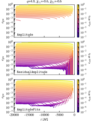
We now consider a more stringent smoothness test: using the same dataset of 50 SEOBNRv4EHM waveforms, we test whether the time evolution of $e_{\text{gw}}$ changes smoothly when varying $e_{\text{eob}}$ at $t_{0}=-20000M$. Figure 11 shows $e_{\text{gw}}(t)$ for the Amplitude, ResidualAmplitude and AmplitudeFits methods. Even though the waveform data starts at $t_{0}=-20000M$, the $e_{\text{gw}}(t)$ is only available for $t\geq\widehat{t}_{0}$, the maximum of the times of the first pericenter and apocenter. In Fig. 9 only eccentricities at the first available time $e_{\text{gw}}(\widehat{t}_{0})$ are considered, while in Fig. 11 we consider the full time evolution.

In Fig. 11, we once again find that the Amplitude method breaks down for small eccentricities $e_{\text{gw}}\lesssim 10^{-3}\ldots 10^{-2}$, especially as one approaches the merger as eccentricity is continuously radiated away. The Amplitude method fails when the local extrema in $A_{22}$ cease to exist, which is why the curves with smaller initial $e_{\text{gw}}$ are shorter. By contrast, the ResidualAmplitude and AmplitudeFits methods continue to compute the eccentricity until $e_{\text{gw}}\sim 10^{-5}$. While the ResidualAmplitude method successfully computes $e_{\text{gw}}(t)$ up to the last available orbit (we discard the last two orbits before the merger as explained in Sec. II.3), the AmplitudeFits method misses some extrema near the merger, especially when the eccentricity becomes small. However, as we will see below, the ResidualAmplitude method can depend on the choice of the quasicircular waveform in the same region.

Figure 13: Differences in $e_{\text{gw}}(t)$ due to different methods used to locate pericenters and apocenters, for the same SEOBNRv4EHM waveforms as Fig. 11. Top-left: The curves show $e_{\text{gw}}(t)$ obtained using the ResidualAmplitude method with the quasicircular counterpart also obtained from SEOBNRv4EHM. The colors represent the absolute difference with respect to the $e_{\text{gw}}(t)$ obtained using the AmplitudeFits method, and the gray region shows the parts where the second method fails to compute $e_{\text{gw}}(t)$. Top-right: Same, but now the colors show the difference with respect to the $e_{\text{gw}}(t)$ obtained with ResidualAmplitude method with the quasicircular counterpart obtained from the IMRPhenomT model. In both top panels, the different choices for locating pericenters/apocenters lead to broadly consistent results for $e_{\text{gw}}(t)$, with the only notable differences occurring for: (i) small eccentricities ($e_{\text{gw}}\lesssim 5\!\times\!10^{-3}$) and near the merger, where the SEOBNRv4EHM model also has known issues (see Fig. 12), and (ii) large eccentricities ($e_{\text{gw}}\sim 0.9$), where locating apocenters is problematic. The bottom panels show the same as the top panels, but when identifying the midpoints between pericenters as apocenters. This leads to more consistent results between different methods, and the largest differences in $e_{\text{gw}}$ decrease by an order of magnitude.

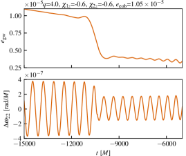
In most regions of Fig. 11, we find that the time evolution of $e_{\text{gw}}$ varies smoothly with $e_{\text{eob}}$. However, for the ResidualAmplitude and AmplitudeFits methods, for small eccentricities and near the merger, we find that $e_{\text{gw}}(t)$ can be noisy. Rather than a limitation of these methods, this behavior arises from the SEOBNRv4EHM model itself. Figure 12 focuses on one of the noisy $e_{\text{gw}}(t)$ curves from the middle panel of Fig. 11. The bottom panel of Fig. 12 shows the corresponding $\Delta\omega_{22}(t)$ from Eq. (26), which helps highlight the modulations due to eccentricity. The fall in $e_{\text{gw}}(t)$ is associated with an abrupt fall in the amplitude of the eccentricity modulations in $\Delta\omega_{22}(t)$.

Such jumps in $\Delta\omega_{22}(t)$ at small eccentricities arise from a transition function in SEOBNRv4EHM Ramos-Buades et al. (2022a) that orbit averages the dynamical variables entering the non quasicircular (NQC) corrections of the waveform. The orbit average is carried out between the local maxima of the oscillations in $\dot{p}_{r^{*}}$ (see Appendix B of Ref. Ramos-Buades et al. (2022a) for details). After the last available maximum, a window is applied to transition from the orbit-averaged variables to the plunge dynamics (see Eq. (B2) in Appendix B of Ref. Ramos-Buades et al. (2022a)). This transition causes the jump in $\Delta\omega_{22}$ shown in Fig. 12, as well as the noisy features at small eccentricity in Fig. 11. Because the last available maximum occurs at earlier times for smaller eccentricities —analogous to Eq. (25)—, these features also start at earlier times for smaller eccentricities in Fig. 11. While this behavior is noticeable in our studies, Ref. Ramos-Buades et al. (2023) shows that this causes no significant biases in parameter estimation, and can be addressed in future versions of SEOBNRv4EHM. Nevertheless, Fig. 11 once again highlights the importance of such smoothness tests, not only to check our implementation of $e_{\text{gw}}$ but also to identify potential issues in waveform models.

IV.4 Dependence of $e_{\text{gw}}$ on extrema finding methods

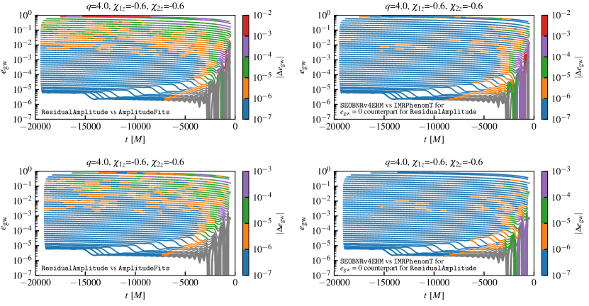
For the final robustness test, we consider how strongly $e_{\text{gw}}$ depends on the method used to locate extrema. We will only consider the ResidualAmplitude and AmplitudeFits methods for simplicity. From Figs. 9 and 11, we already see that $e_{\text{gw}}$ is broadly consistent between different methods. We now quantify the differences in Fig. 13, for the same dataset of 50 SEOBNRv4EHM waveforms from Sec. IV.3.

The top-left panel of Fig. 13 shows $e_{\text{gw}}(t)$ for these waveforms when using the ResidualAmplitude method and the colors represent the instantaneous absolute difference with respect to the $e_{\text{gw}}(t)$ obtained from the AmplitudeFits method. Here, we use SEOBNRv4EHM evaluated at zero eccentricity for the quasicircular counterpart required for ResidualAmplitude. The gray region represents the parts where ResidualAmplitude can compute $e_{\text{gw}}(t)$, but AmplitudeFits can not. However, we note that this only occurs for small eccentricities $e_{\text{gw}}\lesssim 5\!\times\!10^{-3}$, and close to the merger. This region also coincides with the region where SEOBNRv4EHM exhibits the noisy behavior discussed in Fig. 12.

Next, the top-right panel of Fig. 13 illustrates the difference in $e_{\text{gw}}(t)$ between different choices of quasicircular counterpart for the ResidualAmplitude method. The curves once again represent $e_{\text{gw}}(t)$ evaluated using ResidualAmplitude with the quasicircular counterpart obtained from SEOBNRv4EHM (the same model used to produce the eccentric waveforms). The colors represent the instantaneous absolute difference with respect to the $e_{\text{gw}}(t)$ obtained from the ResidualAmplitude method with the quasicircular counterpart obtained from the IMRPhenomT model instead. The gray region represents the parts where ResidualAmplitude using SEOBNRv4EHM for the quasicircular counterpart can compute $e_{\text{gw}}(t)$, but ResidualAmplitude using IMRPhenomT can not. Once again, this occurs only for small eccentricities and near the merger. In this regime, the small differences between SEOBNRv4EHM (in the quasicircular limit) and IMRPhenomT, especially near the merger, become important, and IMRPhenomT does not accurately capture the secular growth in SEOBNRv4EHM.

In the regions where both ResidualAmplitude and AmplitudeFits methods successfully compute $e_{\text{gw}}(t)$ in the top-left panel of Fig. 13, the biggest differences are of order $10^{-2}$. These differences occur either for small eccentricities near the merger, or for very large eccentricities ($e_{\text{gw}}\sim 0.9$). At such high eccentricities, the waveform is characterized by sharp bursts at pericenter passages alternating with wide valleys that include the apocenter passages (see bottom panel of Fig. 2, for example). As a result, it is easy to identify the pericenter times but not the apocenter times for these waveforms. This can be resolved by only identifying the pericenter times and defining the apocenter times to be the midpoints between consecutive pericenters. The assumption employed here is that the radiation reaction is not strong enough that the times taken for the first and second halves of an orbit are significantly different. While this assumption is broken near the merger, we already discard the last two orbits before the merger when computing $e_{\text{gw}}$ (Sec. II.3).

The bottom panels of Fig. 13 show the same as the top panels, but when identifying the midpoints between pericenters as apocenters. We find that the largest differences between ResidualAmplitude and AmplitudeFits, as well as the largest differences between ResidualAmplitude with different quasicircular counterparts, are now an order of magnitude smaller. This suggests that identifying the midpoints between pericenters as apocenters may be a more robust choice than directly locating apocenters, especially for large eccentricities. We provide this as an option in gw_eccentricity Shaikh et al. .

To summarize, the different choices for locating extrema in Fig. 13 lead to broadly consistent results for $e_{\text{gw}}(t)$, with the only notable differences occurring for: (i) small eccentricities ($e_{\text{gw}}\lesssim 5\!\times\!10^{-3}$) and near the merger, where the SEOBNRv4EHM model also has known issues (see Fig. 12), and (ii) large eccentricities ($e_{\text{gw}}\sim 0.9$), where locating apocenters is problematic. As discussed in Sec. III, such differences are expected, and the different methods to locate extrema should be regarded as different definitions of eccentricity. However, identifying the midpoints between pericenters as apocenters, rather than directly locating apocenters, can lead to more consistent results between different methods.

IV.5 Applicability for the high eccentricity regime

Figure 14: A smoothness test for $e_{\text{gw}}(t)$ at very high eccentricities. The curves show the time evolution of $e_{\text{gw}}$ for SEOBNRv4EHM waveforms with initial eccentricities $0.9\leq e_{\text{eob}}\leq 0.999$ at $t_{0}=-5\!\times\!10^{6}M$. The colors represent $e_{\text{eob}}$ at $t_{0}$. The binary parameters are shown in the figure title. We use the ResidualAmplitude method to locate pericenters and identify the midpoints between pericenters as apocenters.

The tests we have conducted so far have been restricted to $e_{\text{gw}}\leq 0.9$. In this section, we focus on testing our implementation in the high eccentricity regime, $e_{\text{gw}}>0.9$. While the eccentricity definition adopted in this work is, in principle, valid at all eccentricities in the range $(0-1)$, high eccentricity comes with additional challenges:

• As $e_{\text{gw}}\to 1$, the separation in time between pericenters increases (see Fig. 2), making it challenging to produce waveforms with enough extrema to construct the $\omega^{\text{p}}_{22}(t)$ and $\omega^{\text{a}}_{22}(t)$ interpolants required in Eq. (4). This limits the practical applicability of $e_{\text{gw}}$ for high-eccentricity NR simulations like those in Ref. Healy and Lousto (2022). However, as we will see below, if sufficiently long waveforms can be produced, this definition of eccentricity and our implementation still work at high eccentricities.

• The first available time $\widehat{t}_{0}$ for $e_{\text{gw}}(t)$, is the maximum of the times of the first pericenter and first apocenter (Sec. II.3), which occurs up to an orbit after the start of the waveform, $t_{0}$. As the duration of orbits increases with eccentricity, so does the difference between $t_{0}$ and $\widehat{t}_{0}$. As eccentricity also evolves during this time, a non-negligible amount of eccentricity may be radiated away before the first available time for the $e_{\text{gw}}(t)$ measurement (see an example below).

• As discussed in Sec. IV.4, locating apocenters becomes challenging at high eccentricities. Therefore, in the test below, we identify the midpoints between pericenters as apocenters, rather than directly locating apocenters.

To test our implementation at high eccentricities, we construct a new dataset of SEOBNRv4EHM waveforms with eccentricities $0.9\leq e_{\text{eob}}\leq 0.999$ defined at $t_{0}=-5\!\times\!10^{6}M$,  for a system with parameters $q=1$, and $\chi_{1z}=\chi_{2z}=0$. For this dataset, the waveforms include 154 (672) pericenters before merger for $e_{\text{eob}}=0.999$ ($e_{\text{eob}}=0.9$) at $t_{0}$, allowing us to easily measure $e_{\text{gw}}(t)$ even for such high eccentricities. Figure 14 shows the eccentricities $e_{\text{gw}}(t)$ measured using these waveforms; as expected, $e_{\text{gw}}(t)$ varies smoothly with varying $e_{\text{eob}}$ even for high eccentricities. For the waveform with $e_{\text{eob}}=0.999$ at $t_{0}$, the measured eccentricity at the first available time $\widehat{t}_{0}\approx-2\!\times\!10^{6}M$ is $e_{\text{gw}}\approx 0.99$. Because the gap between $\widehat{t}_{0}$ and $t_{0}$ is very large ($\mathchar 21016\relax\,3\!\times\!10^{6}M$) for this case, it is unsurprising that the eccentricity decays to $e_{\text{gw}}(\widehat{t}_{0})=0.99$. The choice of $t_{0}=-5\!\times\!10^{6}M$ was made for this dataset so that $t_{0}$ occurs early in the inspiral, where this decay is less drastic.

V Conclusion

We present a robust implementation of standardized definitions of eccentricity ($e_{\text{gw}}$) and mean anomaly ($l_{\text{gw}}$) that are computed directly from the gravitational waveform (Sec. II). Our method is free of gauge ambiguities, has the correct Newtonian limit, and is applicable for waveforms of all origins, over the full range of allowed eccentricities for bound orbits. However, as our method relies on computing the frequency at pericenter and apocenter passages, it requires waveforms with at least $\mathchar 21016\relax\,4-5$ orbits.

Our method can be applied directly during source parameter estimation or as a postprocessing step to convert posterior samples from the internal definitions used by models and simulations to the standardized ones. This puts all models and simulations on the same footing, while also helping connect GW observations to astrophysical predictions for GW populations. Finally, we propose how the reference frequency $f_{\text{ref}}$ and start frequency $f_{\text{low}}$, that are used in GW data analysis, should be generalized for eccentric binaries (Secs. II.5, II.6, II.7).

One key aspect of computing $e_{\text{gw}}$ and $l_{\text{gw}}$ is identifying the times of pericenter and apocenter passages from the waveform. We provide different methods for this purpose, that should be treated as different variants of the eccentricity definition. Among the provided methods (see Sec. III), the Amplitude method is applicable when eccentricity is sufficiently high ($e_{\text{gw}}\gtrsim 10^{-3}\ldots 10^{-2}$), while ResidualAmplitude and AmplitudeFits are applicable for smaller eccentricities as well.

We demonstrate the robustness of our implementation by testing against waveforms of different origins, including PN, EOB, EMRIs and NR (Sec. IV.2). We further conduct smoothness tests that have the added benefit of identifying noisy features in waveform models (Sec. IV.3). Our tests include waveforms with eccentricities ranging from $10^{-5}$ to 0.999. We discuss the limitations of our approach for very high eccentricities (Sec. IV.5), especially for NR simulations where including $\mathchar 21016\relax\,4-5$ orbits can be challenging when eccentricity is high.

We make our implementation publicly available through an easy-to-use Python package, gw_eccentricity Shaikh et al. . This work focuses on systems without spin-precession, and the most important next step is to generalize our methods to spin-precessing eccentric binaries. We leave this to future work but discuss potential approaches (Sec. II.3.1).

References

- Aasi et al. (2015) J. Aasi et al. (LIGO Scientific), “Advanced LIGO,” Class. Quant. Grav. 32, 074001 (2015), arXiv:1411.4547 [gr-qc] .
- Acernese et al. (2015) F. Acernese et al. (Virgo), “Advanced Virgo: a second-generation interferometric gravitational wave detector,” Class. Quant. Grav. 32, 024001 (2015), arXiv:1408.3978 [gr-qc] .
- Abbott et al. (2021a) R. Abbott et al. (LIGO Scientific, VIRGO, KAGRA), “GWTC-3: Compact Binary Coalescences Observed by LIGO and Virgo During the Second Part of the Third Observing Run,” (2021a), arXiv:2111.03606 [gr-qc] .
- Abbott et al. (2016) B. P. Abbott et al. (LIGO Scientific, Virgo), “Observation of Gravitational Waves from a Binary Black Hole Merger,” Phys. Rev. Lett. 116, 061102 (2016), arXiv:1602.03837 [gr-qc] .
- Abbott et al. (2017a) Benjamin P. Abbott et al. (LIGO Scientific, Virgo), “GW170817: Observation of Gravitational Waves from a Binary Neutron Star Inspiral,” Phys. Rev. Lett. 119, 161101 (2017a), arXiv:1710.05832 [gr-qc] .
- Abbott et al. (2021b) R. Abbott et al. (LIGO Scientific, KAGRA, VIRGO), “Observation of Gravitational Waves from Two Neutron Star–Black Hole Coalescences,” Astrophys. J. Lett. 915, L5 (2021b), arXiv:2106.15163 [astro-ph.HE] .
- Apostolatos et al. (1994) Theocharis A. Apostolatos, Curt Cutler, Gerald J. Sussman, and Kip S. Thorne, “Spin-induced orbital precession and its modulation of the gravitational waveforms from merging binaries,” Phys. Rev. D 49, 6274–6297 (1994).
- Kidder (1995) Lawrence E. Kidder, “Coalescing binary systems of compact objects to postNewtonian 5/2 order. 5. Spin effects,” Phys. Rev. D 52, 821–847 (1995), arXiv:gr-qc/9506022 .
- Mapelli (2020) Michela Mapelli, “Binary black hole mergers: formation and populations,” Frontiers in Astronomy and Space Sciences 7, 38 (2020), arXiv:2105.12455 [astro-ph.HE] .
- Varma et al. (2019a) Vijay Varma, Scott E. Field, Mark A. Scheel, Jonathan Blackman, Davide Gerosa, Leo C. Stein, Lawrence E. Kidder, and Harald P. Pfeiffer, “Surrogate models for precessing binary black hole simulations with unequal masses,” Phys. Rev. Research. 1, 033015 (2019a), arXiv:1905.09300 [gr-qc] .
- Pratten et al. (2021) Geraint Pratten et al., “Computationally efficient models for the dominant and subdominant harmonic modes of precessing binary black holes,” Phys. Rev. D 103, 104056 (2021), arXiv:2004.06503 [gr-qc] .
- Ossokine et al. (2020) Serguei Ossokine et al., “Multipolar Effective-One-Body Waveforms for Precessing Binary Black Holes: Construction and Validation,” Phys. Rev. D 102, 044055 (2020), arXiv:2004.09442 [gr-qc] .
- Gamba et al. (2022) Rossella Gamba, Sarp Akçay, Sebastiano Bernuzzi, and Jake Williams, “Effective-one-body waveforms for precessing coalescing compact binaries with post-Newtonian twist,” Phys. Rev. D 106, 024020 (2022), arXiv:2111.03675 [gr-qc] .
- Estellés et al. (2022) Héctor Estellés, Marta Colleoni, Cecilio García-Quirós, Sascha Husa, David Keitel, Maite Mateu-Lucena, Maria de Lluc Planas, and Antoni Ramos-Buades, “New twists in compact binary waveform modeling: A fast time-domain model for precession,” Phys. Rev. D 105, 084040 (2022), arXiv:2105.05872 [gr-qc] .
- Hamilton et al. (2021) Eleanor Hamilton, Lionel London, Jonathan E. Thompson, Edward Fauchon-Jones, Mark Hannam, Chinmay Kalaghatgi, Sebastian Khan, Francesco Pannarale, and Alex Vano-Vinuales, “Model of gravitational waves from precessing black-hole binaries through merger and ringdown,” Phys. Rev. D 104, 124027 (2021), arXiv:2107.08876 [gr-qc] .
- Farr et al. (2014) Benjamin Farr, Evan Ochsner, Will M. Farr, and Richard O’Shaughnessy, “A more effective coordinate system for parameter estimation of precessing compact binaries from gravitational waves,” Phys. Rev. D 90, 024018 (2014), arXiv:1404.7070 [gr-qc] .
- Romero-Shaw et al. (2020a) I. M. Romero-Shaw et al., “Bayesian inference for compact binary coalescences with bilby: validation and application to the first LIGO–Virgo gravitational-wave transient catalogue,” Mon. Not. Roy. Astron. Soc. 499, 3295–3319 (2020a), arXiv:2006.00714 [astro-ph.IM] .
- Veitch et al. (2015) J. Veitch et al., “Robust parameter estimation for compact binaries with ground-based gravitational-wave observations using the LALInference software library,” Phys. Rev. D 91, 042003 (2015), arXiv:1409.7215 [gr-qc] .
- Peters and Mathews (1963) P. C. Peters and J. Mathews, “Gravitational radiation from point masses in a Keplerian orbit,” Phys. Rev. 131, 435–439 (1963).
- Peters (1964) P. C. Peters, “Gravitational Radiation and the Motion of Two Point Masses,” Phys. Rev. 136, B1224–B1232 (1964).
- Blanchet (2014) Luc Blanchet, “Gravitational Radiation from Post-Newtonian Sources and Inspiralling Compact Binaries,” Living Rev. Rel. 17, 2 (2014), arXiv:1310.1528 [gr-qc] .
- Naoz (2016) Smadar Naoz, “The Eccentric Kozai-Lidov Effect and Its Applications,” Annual Review of Astronomy and Astrophysics 54, 441–489 (2016), arXiv:1601.07175 [astro-ph.EP] .
- Martinez et al. (2020) Miguel A. S. Martinez, Giacomo Fragione, Kyle Kremer, Sourav Chatterjee, Carl L. Rodriguez, Johan Samsing, Claire S. Ye, Newlin C. Weatherford, Michael Zevin, Smadar Naoz, and Frederic A. Rasio, “Black Hole Mergers from Hierarchical Triples in Dense Star Clusters,” The Astrophysical Journal 903, 67 (2020), arXiv:2009.08468 [astro-ph.GA] .
- Romero-Shaw et al. (2019) Isobel M. Romero-Shaw, Paul D. Lasky, and Eric Thrane, “Searching for Eccentricity: Signatures of Dynamical Formation in the First Gravitational-Wave Transient Catalogue of LIGO and Virgo,” Mon. Not. Roy. Astron. Soc. 490, 5210–5216 (2019), arXiv:1909.05466 [astro-ph.HE] .
- Romero-Shaw et al. (2020b) Isobel M. Romero-Shaw, Paul D. Lasky, Eric Thrane, and Juan Calderon Bustillo, “GW190521: orbital eccentricity and signatures of dynamical formation in a binary black hole merger signal,” Astrophys. J. Lett. 903, L5 (2020b), arXiv:2009.04771 [astro-ph.HE] .
- Gayathri et al. (2022) V. Gayathri, J. Healy, J. Lange, B. O’Brien, M. Szczepanczyk, Imre Bartos, M. Campanelli, S. Klimenko, C. O. Lousto, and R. O’Shaughnessy, “Eccentricity estimate for black hole mergers with numerical relativity simulations,” Nature Astron. 6, 344–349 (2022), arXiv:2009.05461 [astro-ph.HE] .
- Calderón Bustillo et al. (2021a) Juan Calderón Bustillo, Nicolas Sanchis-Gual, Alejandro Torres-Forné, José A. Font, Avi Vajpeyi, Rory Smith, Carlos Herdeiro, Eugen Radu, and Samson H. W. Leong, “GW190521 as a Merger of Proca Stars: A Potential New Vector Boson of eV,” Phys. Rev. Lett. 126, 081101 (2021a), arXiv:2009.05376 [gr-qc] .
- Calderón Bustillo et al. (2021b) Juan Calderón Bustillo, Nicolas Sanchis-Gual, Alejandro Torres-Forné, and José A. Font, “Confusing Head-On Collisions with Precessing Intermediate-Mass Binary Black Hole Mergers,” Phys. Rev. Lett. 126, 201101 (2021b), arXiv:2009.01066 [gr-qc] .
- O’Shea and Kumar (2021) Eamonn O’Shea and Prayush Kumar, “Correlations in parameter estimation of low-mass eccentric binaries: GW151226 & GW170608,” (2021), arXiv:2107.07981 [astro-ph.HE] .
- Gamba et al. (2023) Rossella Gamba, Matteo Breschi, Gregorio Carullo, Simone Albanesi, Piero Rettegno, Sebastiano Bernuzzi, and Alessandro Nagar, “GW190521 as a dynamical capture of two nonspinning black holes,” Nature Astron. 7, 11–17 (2023), arXiv:2106.05575 [gr-qc] .
- Romero-Shaw et al. (2022) Isobel M. Romero-Shaw, Paul D. Lasky, and Eric Thrane, “Four Eccentric Mergers Increase the Evidence that LIGO–Virgo–KAGRA’s Binary Black Holes Form Dynamically,” Astrophys. J. 940, 171 (2022), arXiv:2206.14695 [astro-ph.HE] .
- Akutsu et al. (2021) T. Akutsu et al. (KAGRA), “Overview of KAGRA: Detector design and construction history,” PTEP 2021, 05A101 (2021), arXiv:2005.05574 [physics.ins-det] .
- Abbott et al. (2018) B. P. Abbott et al. (KAGRA, LIGO Scientific, VIRGO), “Prospects for Observing and Localizing Gravitational-Wave Transients with Advanced LIGO, Advanced Virgo and KAGRA,” Living Rev. Rel. 21, 3 (2018), arXiv:1304.0670 [gr-qc] .
- Punturo et al. (2010) M. Punturo et al., “The Einstein Telescope: A third-generation gravitational wave observatory,” Proceedings, 14th Workshop on Gravitational wave data analysis (GWDAW-14): Rome, Italy, January 26-29, 2010, Class. Quant. Grav. 27, 194002 (2010).
- Hild et al. (2011) S. Hild et al., “Sensitivity Studies for Third-Generation Gravitational Wave Observatories,” Class. Quant. Grav. 28, 094013 (2011), arXiv:1012.0908 [gr-qc] .
- Abbott et al. (2017b) Benjamin P Abbott et al. (LIGO Scientific), “Exploring the Sensitivity of Next Generation Gravitational Wave Detectors,” Class. Quant. Grav. 34, 044001 (2017b), arXiv:1607.08697 [astro-ph.IM] .
- Reitze et al. (2019) David Reitze et al., “Cosmic Explorer: The U.S. Contribution to Gravitational-Wave Astronomy beyond LIGO,” Bull. Am. Astron. Soc. 51, 035 (2019), arXiv:1907.04833 [astro-ph.IM] .
- Sesana (2016) Alberto Sesana, “Prospects for Multiband Gravitational-Wave Astronomy after GW150914,” Phys. Rev. Lett. 116, 231102 (2016), arXiv:1602.06951 [gr-qc] .
- Seoane et al. (2023) Pau Amaro Seoane et al. (LISA), “Astrophysics with the Laser Interferometer Space Antenna,” Living Rev. Rel. 26, 2 (2023), arXiv:2203.06016 [gr-qc] .
- Klein et al. (2022) Antoine Klein et al., “The last three years: multiband gravitational-wave observations of stellar-mass binary black holes,” (2022), arXiv:2204.03423 [astro-ph.HE] .
- Bonetti et al. (2018) Matteo Bonetti, Francesco Haardt, Alberto Sesana, and Enrico Barausse, “Post-Newtonian evolution of massive black hole triplets in galactic nuclei – II. Survey of the parameter space,” Mon. Not. Roy. Astron. Soc. 477, 3910–3926 (2018), arXiv:1709.06088 [astro-ph.GA] .
- Warburton et al. (2012) Niels Warburton, Sarp Akcay, Leor Barack, Jonathan R. Gair, and Norichika Sago, “Evolution of inspiral orbits around a Schwarzschild black hole,” Phys. Rev. D 85, 061501 (2012), arXiv:1111.6908 [gr-qc] .
- Osburn et al. (2016) Thomas Osburn, Niels Warburton, and Charles R. Evans, “Highly eccentric inspirals into a black hole,” Phys. Rev. D 93, 064024 (2016), arXiv:1511.01498 [gr-qc] .
- Cao and Han (2017) Zhoujian Cao and Wen-Biao Han, “Waveform model for an eccentric binary black hole based on the effective-one-body-numerical-relativity formalism,” Phys. Rev. D 96, 044028 (2017), arXiv:1708.00166 [gr-qc] .
- Liu et al. (2020) Xiaolin Liu, Zhoujian Cao, and Lijing Shao, “Validating the Effective-One-Body Numerical-Relativity Waveform Models for Spin-aligned Binary Black Holes along Eccentric Orbits,” Phys. Rev. D 101, 044049 (2020), arXiv:1910.00784 [gr-qc] .
- Ramos-Buades et al. (2022a) Antoni Ramos-Buades, Alessandra Buonanno, Mohammed Khalil, and Serguei Ossokine, “Effective-one-body multipolar waveforms for eccentric binary black holes with nonprecessing spins,” Phys. Rev. D 105, 044035 (2022a), arXiv:2112.06952 [gr-qc] .
- Nagar et al. (2021) Alessandro Nagar, Alice Bonino, and Piero Rettegno, “Effective one-body multipolar waveform model for spin-aligned, quasicircular, eccentric, hyperbolic black hole binaries,” Phys. Rev. D 103, 104021 (2021), arXiv:2101.08624 [gr-qc] .
- Islam et al. (2021) Tousif Islam, Vijay Varma, Jackie Lodman, Scott E. Field, Gaurav Khanna, Mark A. Scheel, Harald P. Pfeiffer, Davide Gerosa, and Lawrence E. Kidder, “Eccentric binary black hole surrogate models for the gravitational waveform and remnant properties: comparable mass, nonspinning case,” Phys. Rev. D 103, 064022 (2021), arXiv:2101.11798 [gr-qc] .
- Liu et al. (2022) Xiaolin Liu, Zhoujian Cao, and Zong-Hong Zhu, “A higher-multipole gravitational waveform model for an eccentric binary black holes based on the effective-one-body-numerical-relativity formalism,” Class. Quant. Grav. 39, 035009 (2022), arXiv:2102.08614 [gr-qc] .
- Memmesheimer et al. (2004) Raoul-Martin Memmesheimer, Achamveedu Gopakumar, and Gerhard Schaefer, “Third post-Newtonian accurate generalized quasi-Keplerian parametrization for compact binaries in eccentric orbits,” Phys. Rev. D 70, 104011 (2004), arXiv:gr-qc/0407049 .
- Huerta et al. (2014) E. A. Huerta, Prayush Kumar, Sean T. McWilliams, Richard O’Shaughnessy, and Nicolás Yunes, “Accurate and efficient waveforms for compact binaries on eccentric orbits,” Phys. Rev. D 90, 084016 (2014), arXiv:1408.3406 [gr-qc] .
- Tanay et al. (2016) Sashwat Tanay, Maria Haney, and Achamveedu Gopakumar, “Frequency and time domain inspiral templates for comparable mass compact binaries in eccentric orbits,” Phys. Rev. D 93, 064031 (2016), arXiv:1602.03081 [gr-qc] .
- Cho et al. (2022) Gihyuk Cho, Sashwat Tanay, Achamveedu Gopakumar, and Hyung Mok Lee, “Generalized quasi-Keplerian solution for eccentric, nonspinning compact binaries at 4PN order and the associated inspiral-merger-ringdown waveform,” Phys. Rev. D 105, 064010 (2022), arXiv:2110.09608 [gr-qc] .
- Moore et al. (2018) Blake Moore, Travis Robson, Nicholas Loutrel, and Nicolas Yunes, “Towards a Fourier domain waveform for non-spinning binaries with arbitrary eccentricity,” Class. Quant. Grav. 35, 235006 (2018), arXiv:1807.07163 [gr-qc] .
- Moore and Yunes (2019) Blake Moore and Nicolás Yunes, “A 3PN Fourier Domain Waveform for Non-Spinning Binaries with Moderate Eccentricity,” Class. Quant. Grav. 36, 185003 (2019), arXiv:1903.05203 [gr-qc] .
- van de Meent and Warburton (2018) Maarten van de Meent and Niels Warburton, “Fast Self-forced Inspirals,” Class. Quant. Grav. 35, 144003 (2018), arXiv:1802.05281 [gr-qc] .
- Chua et al. (2021) Alvin J. K. Chua, Michael L. Katz, Niels Warburton, and Scott A. Hughes, “Rapid generation of fully relativistic extreme-mass-ratio-inspiral waveform templates for LISA data analysis,” Phys. Rev. Lett. 126, 051102 (2021), arXiv:2008.06071 [gr-qc] .
- Hughes et al. (2021) Scott A. Hughes, Niels Warburton, Gaurav Khanna, Alvin J. K. Chua, and Michael L. Katz, “Adiabatic waveforms for extreme mass-ratio inspirals via multivoice decomposition in time and frequency,” Phys. Rev. D 103, 104014 (2021), arXiv:2102.02713 [gr-qc] .
- Katz et al. (2021) Michael L. Katz, Alvin J. K. Chua, Lorenzo Speri, Niels Warburton, and Scott A. Hughes, “Fast extreme-mass-ratio-inspiral waveforms: New tools for millihertz gravitational-wave data analysis,” Phys. Rev. D 104, 064047 (2021), arXiv:2104.04582 [gr-qc] .
- Lynch et al. (2022) Philip Lynch, Maarten van de Meent, and Niels Warburton, “Eccentric self-forced inspirals into a rotating black hole,” Class. Quant. Grav. 39, 145004 (2022), arXiv:2112.05651 [gr-qc] .
- Klein (2021) Antoine Klein, “EFPE: Efficient fully precessing eccentric gravitational waveforms for binaries with long inspirals,” (2021), arXiv:2106.10291 [gr-qc] .
- Barack and Sago (2010) Leor Barack and Norichika Sago, “Gravitational self-force on a particle in eccentric orbit around a Schwarzschild black hole,” Phys. Rev. D 81, 084021 (2010), arXiv:1002.2386 [gr-qc] .
- Akcay et al. (2013) Sarp Akcay, Niels Warburton, and Leor Barack, “Frequency-domain algorithm for the Lorenz-gauge gravitational self-force,” Phys. Rev. D 88, 104009 (2013), arXiv:1308.5223 [gr-qc] .
- Hopper and Evans (2013) Seth Hopper and Charles R. Evans, “Metric perturbations from eccentric orbits on a Schwarzschild black hole: I. Odd-parity Regge-Wheeler to Lorenz gauge transformation and two new methods to circumvent the Gibbs phenomenon,” Phys. Rev. D 87, 064008 (2013), arXiv:1210.7969 [gr-qc] .
- Osburn et al. (2014) Thomas Osburn, Erik Forseth, Charles R. Evans, and Seth Hopper, “Lorenz gauge gravitational self-force calculations of eccentric binaries using a frequency domain procedure,” Phys. Rev. D 90, 104031 (2014), arXiv:1409.4419 [gr-qc] .
- van de Meent and Shah (2015) Maarten van de Meent and Abhay G. Shah, “Metric perturbations produced by eccentric equatorial orbits around a Kerr black hole,” Phys. Rev. D 92, 064025 (2015), arXiv:1506.04755 [gr-qc] .
- Hopper et al. (2016) Seth Hopper, Chris Kavanagh, and Adrian C. Ottewill, “Analytic self-force calculations in the post-Newtonian regime: eccentric orbits on a Schwarzschild background,” Phys. Rev. D 93, 044010 (2016), arXiv:1512.01556 [gr-qc] .
- Forseth et al. (2016) Erik Forseth, Charles R. Evans, and Seth Hopper, “Eccentric-orbit extreme-mass-ratio inspiral gravitational wave energy fluxes to 7PN order,” Phys. Rev. D 93, 064058 (2016), arXiv:1512.03051 [gr-qc] .
- van de Meent (2016) Maarten van de Meent, “Gravitational self-force on eccentric equatorial orbits around a Kerr black hole,” Phys. Rev. D 94, 044034 (2016), arXiv:1606.06297 [gr-qc] .
- van de Meent (2018) Maarten van de Meent, “Gravitational self-force on generic bound geodesics in Kerr spacetime,” Phys. Rev. D 97, 104033 (2018), arXiv:1711.09607 [gr-qc] .
- Munna et al. (2020) Christopher Munna, Charles R. Evans, Seth Hopper, and Erik Forseth, “Determination of new coefficients in the angular momentum and energy fluxes at infinity to 9PN order for eccentric Schwarzschild extreme-mass-ratio inspirals using mode-by-mode fitting,” Phys. Rev. D 102, 024047 (2020), arXiv:2005.03044 [gr-qc] .
- Munna and Evans (2020) Christopher Munna and Charles R. Evans, “Eccentric-orbit extreme-mass-ratio-inspiral radiation II: 1PN correction to leading-logarithm and subleading-logarithm flux sequences and the entire perturbative 4PN flux,” Phys. Rev. D 102, 104006 (2020), arXiv:2009.01254 [gr-qc] .
- Munna and Evans (2022a) Christopher Munna and Charles R. Evans, “High-order post-Newtonian expansion of the redshift invariant for eccentric-orbit nonspinning extreme-mass-ratio inspirals,” Phys. Rev. D 106, 044004 (2022a), arXiv:2203.13832 [gr-qc] .
- Munna and Evans (2022b) Christopher Munna and Charles R. Evans, “Post-Newtonian expansion of the spin-precession invariant for eccentric-orbit nonspinning extreme-mass-ratio inspirals to 9PN and e16,” Phys. Rev. D 106, 044058 (2022b), arXiv:2206.04085 [gr-qc] .
- Hinder et al. (2018) Ian Hinder, Lawrence E. Kidder, and Harald P. Pfeiffer, “Eccentric binary black hole inspiral-merger-ringdown gravitational waveform model from numerical relativity and post-Newtonian theory,” Phys. Rev. D 98, 044015 (2018), arXiv:1709.02007 [gr-qc] .
- Boyle et al. (2019) Michael Boyle et al., “The SXS Collaboration catalog of binary black hole simulations,” Class. Quant. Grav. 36, 195006 (2019), arXiv:1904.04831 [gr-qc] .
- Ramos-Buades et al. (2022b) Antoni Ramos-Buades, Maarten van de Meent, Harald P. Pfeiffer, Hannes R. Rüter, Mark A. Scheel, Michael Boyle, and Lawrence E. Kidder, “Eccentric binary black holes: Comparing numerical relativity and small mass-ratio perturbation theory,” Phys. Rev. D 106, 124040 (2022b), arXiv:2209.03390 [gr-qc] .
- Healy and Lousto (2022) James Healy and Carlos O. Lousto, “Fourth RIT binary black hole simulations catalog: Extension to eccentric orbits,” Phys. Rev. D 105, 124010 (2022), arXiv:2202.00018 [gr-qc] .
- Habib and Huerta (2019) Sarah Habib and E. A. Huerta, “Characterization of numerical relativity waveforms of eccentric binary black hole mergers,” Phys. Rev. D 100, 044016 (2019), arXiv:1904.09295 [gr-qc] .
- Huerta et al. (2019) E. A. Huerta et al., “Physics of eccentric binary black hole mergers: A numerical relativity perspective,” Phys. Rev. D 100, 064003 (2019), arXiv:1901.07038 [gr-qc] .
- Joshi et al. (2023) Abhishek V. Joshi, Shawn G. Rosofsky, Roland Haas, and E. A. Huerta, “Numerical relativity higher order gravitational waveforms of eccentric, spinning, nonprecessing binary black hole mergers,” Phys. Rev. D 107, 064038 (2023), arXiv:2210.01852 [gr-qc] .
- Abbott et al. (2017c) Benjamin P. Abbott et al. (LIGO Scientific, Virgo), “Effects of waveform model systematics on the interpretation of GW150914,” Class. Quant. Grav. 34, 104002 (2017c), arXiv:1611.07531 [gr-qc] .
- Lower et al. (2018) Marcus E. Lower, Eric Thrane, Paul D. Lasky, and Rory Smith, “Measuring eccentricity in binary black hole inspirals with gravitational waves,” Phys. Rev. D 98, 083028 (2018), arXiv:1806.05350 [astro-ph.HE] .
- Ramos-Buades et al. (2020a) Antoni Ramos-Buades, Sascha Husa, Geraint Pratten, Héctor Estellés, Cecilio García-Quirós, Maite Mateu-Lucena, Marta Colleoni, and Rafel Jaume, “First survey of spinning eccentric black hole mergers: Numerical relativity simulations, hybrid waveforms, and parameter estimation,” Phys. Rev. D 101, 083015 (2020a), arXiv:1909.11011 [gr-qc] .
- Ramos-Buades et al. (2020b) Antoni Ramos-Buades, Shubhanshu Tiwari, Maria Haney, and Sascha Husa, “Impact of eccentricity on the gravitational wave searches for binary black holes: High mass case,” Phys. Rev. D 102, 043005 (2020b), arXiv:2005.14016 [gr-qc] .
- Romero-Shaw et al. (2023) Isobel M. Romero-Shaw, Davide Gerosa, and Nicholas Loutrel, “Eccentricity or spin precession? Distinguishing subdominant effects in gravitational-wave data,” Mon. Not. Roy. Astron. Soc. 519, 5352–5357 (2023), arXiv:2211.07528 [astro-ph.HE] .
- Knee et al. (2022) Alan M. Knee, Isobel M. Romero-Shaw, Paul D. Lasky, Jess McIver, and Eric Thrane, “A Rosetta Stone for Eccentric Gravitational Waveform Models,” Astrophys. J. 936, 172 (2022), arXiv:2207.14346 [gr-qc] .
- Bonino et al. (2023) Alice Bonino, Rossella Gamba, Patricia Schmidt, Alessandro Nagar, Geraint Pratten, Matteo Breschi, Piero Rettegno, and Sebastiano Bernuzzi, “Inferring eccentricity evolution from observations of coalescing binary black holes,” Phys. Rev. D 107, 064024 (2023), arXiv:2207.10474 [gr-qc] .
- Yang et al. (2022) Tao Yang, Rong-Gen Cai, Zhoujian Cao, and Hyung Mok Lee, “Eccentricity of Long Inspiraling Compact Binaries Sheds Light on Dark Sirens,” Phys. Rev. Lett. 129, 191102 (2022), arXiv:2202.08608 [gr-qc] .
- Schmidt et al. (2017) Patricia Schmidt, Ian W. Harry, and Harald P. Pfeiffer, “Numerical Relativity Injection Infrastructure,” (2017), arXiv:1703.01076 [gr-qc] .
- Clarke et al. (2022) Teagan A. Clarke, Isobel M. Romero-Shaw, Paul D. Lasky, and Eric Thrane, “Gravitational-wave inference for eccentric binaries: the argument of periapsis,” Mon. Not. Roy. Astron. Soc. 517, 3778–3784 (2022), arXiv:2206.14006 [gr-qc] .
- Varma et al. (2022a) Vijay Varma, Maximiliano Isi, Sylvia Biscoveanu, Will M. Farr, and Salvatore Vitale, “Measuring binary black hole orbital-plane spin orientations,” Phys. Rev. D 105, 024045 (2022a), arXiv:2107.09692 [astro-ph.HE] .
- (93) Md Arif Shaikh, Vijay Varma, Harald Pfeiffer, Antoni Ramos-Buades, and Maarten van de Meent, “gw_eccentricity: A python package for measuring eccentricity from gravitational waves,” https://pypi.python.org/pypi/gw_eccentricity/.
- Goldstein et al. (2002) H. Goldstein, C.P. Poole, and J.L. Safko, Classical Mechanics (Addison Wesley, 2002).
- Ossokine et al. (2018) Serguei Ossokine, Tim Dietrich, Evan Foley, Reza Katebi, and Geoffrey Lovelace, “Assessing the Energetics of Spinning Binary Black Hole Systems,” Phys. Rev. D 98, 104057 (2018), arXiv:1712.06533 [gr-qc] .
- Barack and Sago (2011) Leor Barack and Norichika Sago, “Beyond the geodesic approximation: conservative effects of the gravitational self-force in eccentric orbits around a Schwarzschild black hole,” Phys. Rev. D 83, 084023 (2011), arXiv:1101.3331 [gr-qc] .
- Akcay et al. (2015) Sarp Akcay, Alexandre Le Tiec, Leor Barack, Norichika Sago, and Niels Warburton, “Comparison Between Self-Force and Post-Newtonian Dynamics: Beyond Circular Orbits,” Phys. Rev. D 91, 124014 (2015), arXiv:1503.01374 [gr-qc] .
- Akcay et al. (2017) Sarp Akcay, David Dempsey, and Sam R. Dolan, “Spin–orbit precession for eccentric black hole binaries at first order in the mass ratio,” Class. Quant. Grav. 34, 084001 (2017), arXiv:1608.04811 [gr-qc] .
- Hinderer and Babak (2017) Tanja Hinderer and Stanislav Babak, “Foundations of an effective-one-body model for coalescing binaries on eccentric orbits,” Phys. Rev. D 96, 104048 (2017), arXiv:1707.08426 [gr-qc] .
- Chiaramello and Nagar (2020) Danilo Chiaramello and Alessandro Nagar, “Faithful analytical effective-one-body waveform model for spin-aligned, moderately eccentric, coalescing black hole binaries,” Phys. Rev. D 101, 101501 (2020), arXiv:2001.11736 [gr-qc] .
- Khalil et al. (2021) Mohammed Khalil, Alessandra Buonanno, Jan Steinhoff, and Justin Vines, “Radiation-reaction force and multipolar waveforms for eccentric, spin-aligned binaries in the effective-one-body formalism,” Phys. Rev. D 104, 024046 (2021), arXiv:2104.11705 [gr-qc] .
- Buonanno et al. (2011) Alessandra Buonanno, Lawrence E. Kidder, Abdul H. Mroue, Harald P. Pfeiffer, and Andrea Taracchini, “Reducing orbital eccentricity of precessing black-hole binaries,” Phys. Rev. D83, 104034 (2011), arXiv:1012.1549 [gr-qc] .
- Mroue and Pfeiffer (2012) Abdul H. Mroue and Harald P. Pfeiffer, “Precessing Binary Black Holes Simulations: Quasicircular Initial Data,” (2012), arXiv:1210.2958 [gr-qc] .
- Ramos-Buades et al. (2019) Antoni Ramos-Buades, Sascha Husa, and Geraint Pratten, “Simple procedures to reduce eccentricity of binary black hole simulations,” Phys. Rev. D 99, 023003 (2019), arXiv:1810.00036 [gr-qc] .
- Ciarfella et al. (2022) Alessandro Ciarfella, James Healy, Carlos O. Lousto, and Hiroyuki Nakano, “Eccentricity estimation from initial data for numerical relativity simulations,” Phys. Rev. D 106, 104035 (2022), arXiv:2206.13532 [gr-qc] .
- Mora and Will (2002) Thierry Mora and Clifford M. Will, “Numerically generated quasiequilibrium orbits of black holes: Circular or eccentric?” Phys. Rev. D 66, 101501 (2002), arXiv:gr-qc/0208089 .
- Lewis et al. (2017) Adam G. M. Lewis, Aaron Zimmerman, and Harald P. Pfeiffer, “Fundamental frequencies and resonances from eccentric and precessing binary black hole inspirals,” Class. Quant. Grav. 34, 124001 (2017), arXiv:1611.03418 [gr-qc] .
- (108) “Kepler’s laws of planetary motion,” https://en.wikipedia.org/wiki/Kepler’s_laws_of_planetary_motion.
- Winicour (2009) Jeffrey Winicour, “Characteristic Evolution and Matching,” Living Rev. Rel. 12, 3 (2009), arXiv:0810.1903 [gr-qc] .
- Moxon et al. (2020) Jordan Moxon, Mark A. Scheel, and Saul A. Teukolsky, “Improved Cauchy-characteristic evolution system for high-precision numerical relativity waveforms,” Phys. Rev. D 102, 044052 (2020), arXiv:2007.01339 [gr-qc] .
- Reisswig et al. (2007) Christian Reisswig, Nigel T. Bishop, Chi Wai Lai, Jonathan Thornburg, and Bela Szilagyi, “Numerical relativity with characteristic evolution, using six angular patches,” Class. Quant. Grav. 24, S327–S340 (2007), arXiv:gr-qc/0610019 .
- Reisswig et al. (2010) C. Reisswig, N. T. Bishop, D. Pollney, and B. Szilagyi, “Characteristic extraction in numerical relativity: binary black hole merger waveforms at null infinity,” Class. Quant. Grav. 27, 075014 (2010), arXiv:0912.1285 [gr-qc] .
- Reisswig et al. (2013) Christian Reisswig, Nigel T. Bishop, and Denis Pollney, “General relativistic null-cone evolutions with a high-order scheme,” Gen. Rel. Grav. 45, 1069–1094 (2013), arXiv:1208.3891 [gr-qc] .
- Taylor et al. (2013) Nicholas W. Taylor, Michael Boyle, Christian Reisswig, Mark A. Scheel, Tony Chu, Lawrence E. Kidder, and Béla Szilágyi, “Comparing Gravitational Waveform Extrapolation to Cauchy-Characteristic Extraction in Binary Black Hole Simulations,” Phys. Rev. D88, 124010 (2013), arXiv:1309.3605 [gr-qc] .
- Barkett et al. (2020) Kevin Barkett, Jordan Moxon, Mark A. Scheel, and Béla Szilágyi, “Spectral Cauchy-Characteristic Extraction of the Gravitational Wave News Function,” Phys. Rev. D 102, 024004 (2020), arXiv:1910.09677 [gr-qc] .
- Mitman et al. (2022) Keefe Mitman et al., “Fixing the BMS frame of numerical relativity waveforms with BMS charges,” Phys. Rev. D 106, 084029 (2022), arXiv:2208.04356 [gr-qc] .
- (117) SXS Collaboration, “The SXS collaboration catalog of gravitational waveforms,” http://www.black-holes.org/waveforms.
- Boyle et al. (2011) Michael Boyle, Robert Owen, and Harald P. Pfeiffer, “A geometric approach to the precession of compact binaries,” Phys. Rev. D84, 124011 (2011), arXiv:1110.2965 [gr-qc] .
- (119) “Simulating eXtreme Spacetimes,” http://www.black-holes.org/.
- Varma and Ajith (2017) Vijay Varma and Parameswaran Ajith, “Effects of nonquadrupole modes in the detection and parameter estimation of black hole binaries with nonprecessing spins,” Phys. Rev. D96, 124024 (2017), arXiv:1612.05608 [gr-qc] .
- Varma et al. (2014) Vijay Varma, Parameswaran Ajith, Sascha Husa, Juan Calderon Bustillo, Mark Hannam, and Michael Pürrer, “Gravitational-wave observations of binary black holes: Effect of nonquadrupole modes,” Phys. Rev. D90, 124004 (2014), arXiv:1409.2349 [gr-qc] .
- Capano et al. (2014) Collin Capano, Yi Pan, and Alessandra Buonanno, “Impact of higher harmonics in searching for gravitational waves from nonspinning binary black holes,” Phys. Rev. D89, 102003 (2014), arXiv:1311.1286 [gr-qc] .
- Schmidt et al. (2011) Patricia Schmidt, Mark Hannam, Sascha Husa, and P. Ajith, “Tracking the precession of compact binaries from their gravitational-wave signal,” Phys. Rev. D84, 024046 (2011), arXiv:1012.2879 [gr-qc] .
- O’Shaughnessy et al. (2011) R. O’Shaughnessy, B. Vaishnav, J. Healy, Z. Meeks, and D. Shoemaker, “Efficient asymptotic frame selection for binary black hole spacetimes using asymptotic radiation,” Phys. Rev. D84, 124002 (2011), arXiv:1109.5224 [gr-qc] .
- Boyle (2013) Michael Boyle, “Angular velocity of gravitational radiation from precessing binaries and the corotating frame,” Phys. Rev. D87, 104006 (2013), arXiv:1302.2919 [gr-qc] .
- Ramos-Buades et al. (2023) Antoni Ramos-Buades, Alessandra Buonanno, and Jonathan Gair, “Bayesian inference of binary black holes with inspiral-merger-ringdown waveforms using two eccentric parameters,” (2023), arXiv:2309.15528 [gr-qc] .
- Abbott et al. (2023a) R. Abbott et al. (KAGRA, VIRGO, LIGO Scientific), “Population of Merging Compact Binaries Inferred Using Gravitational Waves through GWTC-3,” Phys. Rev. X 13, 011048 (2023a), arXiv:2111.03634 [astro-ph.HE] .
- Varma et al. (2022b) Vijay Varma, Sylvia Biscoveanu, Maximiliano Isi, Will M. Farr, and Salvatore Vitale, “Hints of Spin-Orbit Resonances in the Binary Black Hole Population,” Phys. Rev. Lett. 128, 031101 (2022b), arXiv:2107.09693 [astro-ph.HE] .
- Abbott et al. (2023b) R. Abbott et al. (LIGO Scientific, Virgo, KAGRA), “Constraints on the Cosmic Expansion History from GWTC–3,” Astrophys. J. 949, 76 (2023b), arXiv:2111.03604 [astro-ph.CO] .
- Virtanen et al. (2020) Pauli Virtanen, Ralf Gommers, Travis E. Oliphant, Matt Haberland, Tyler Reddy, David Cournapeau, Evgeni Burovski, Pearu Peterson, Warren Weckesser, Jonathan Bright, Stéfan J. van der Walt, Matthew Brett, Joshua Wilson, K. Jarrod Millman, Nikolay Mayorov, Andrew R. J. Nelson, Eric Jones, Robert Kern, Eric Larson, C J Carey, İlhan Polat, Yu Feng, Eric W. Moore, Jake VanderPlas, Denis Laxalde, Josef Perktold, Robert Cimrman, Ian Henriksen, E. A. Quintero, Charles R. Harris, Anne M. Archibald, Antônio H. Ribeiro, Fabian Pedregosa, Paul van Mulbregt, and SciPy 1.0 Contributors, “SciPy 1.0: Fundamental Algorithms for Scientific Computing in Python,” Nature Methods 17, 261–272 (2020).
- Varma et al. (2019b) Vijay Varma, Scott E. Field, Mark A. Scheel, Jonathan Blackman, Lawrence E. Kidder, and Harald P. Pfeiffer, “Surrogate model of hybridized numerical relativity binary black hole waveforms,” Phys. Rev. D99, 064045 (2019b), arXiv:1812.07865 [gr-qc] .
- Darwin (1959) Charles Darwin, “The Gravity Field of a Particle,” Proceedings of the Royal Society of London Series A 249, 180–194 (1959).
- Darwin (1961) Charles Darwin, “The Gravity Field of a Particle. II,” Proceedings of the Royal Society of London Series A 263, 39–50 (1961).
- (134) http://ccrg.rit.edu/~RITCatalog/.
- Nagar et al. (2018) Alessandro Nagar et al., “Time-domain effective-one-body gravitational waveforms for coalescing compact binaries with nonprecessing spins, tides and self-spin effects,” Phys. Rev. D 98, 104052 (2018), arXiv:1806.01772 [gr-qc] .