Physics-informed Spectral Learning: the Discrete Helmholtz–Hodge Decomposition

Luis Espath♯,1, Pouria Behnoudfar2, & Raúl Tempone3,4,5 1School of Mathematical Sciences, University of Nottingham, Nottingham, NG7 2RD, United Kingdom 2Mineral Resources, Commonwealth Scientific and Industrial Research Organisation (CSIRO), Kensington, Perth, WA 6152, Australia 3Department of Mathematics, RWTH Aachen University, Gebäude-1953 1.OG, Pontdriesch 14-16, 161, 52062 Aachen, Germany. 4Alexander von Humboldt Professor in Mathematics for Uncertainty Quantification, RWTH Aachen University, Germany. 5King Abdullah University of Science & Technology (KAUST), Computer, Electrical and Mathematical Sciences & Engineering Division (CEMSE), Thuwal 23955-6900, Saudi Arabia. espath@gmail.com
Abstract.

In this work, we further develop the Physics-informed Spectral Learning (PiSL) by Espath et al. [1] based on a discrete L2superscript𝐿2L^{2} projection to solve the discrete Hodge–Helmholtz decomposition from sparse data. Within this physics-informed statistical learning framework, we adaptively build a sparse set of Fourier basis functions with corresponding coefficients by solving a sequence of minimization problems where the set of basis functions is augmented greedily at each optimization problem. Moreover, our PiSL  computational framework enjoys spectral (exponential) convergence. We regularize the minimization problems with the seminorm of the fractional Sobolev space in a Tikhonov fashion. In the Fourier setting, the divergence- and curl-free constraints become a finite set of linear algebraic equations. The proposed computational framework combines supervised and unsupervised learning techniques in that we use data concomitantly with the projection onto divergence- and curl-free spaces. We assess the capabilities of our method in various numerical examples including the ‘Storm of the Century’ with satellite data from 1993.
keywords: Physics-informed Machine Learning; Sparse approximation; Statistical learning; Fluid mechanics.
AMS subject classifications: \cdot 76-10 \cdot 68T05 \cdot 30E10 \cdot 35L65 \cdot

1. Introduction

Machine learning is an essential and universal tool for handling and understanding data. Nonetheless, machine learning capabilities are not restricted to generating data-driven models. Various fluid flow applications have been extensively developed in recent years. Particular attention has been focused on Physics-informed Neural Networks (PiNNs) [2, 3] in a statistical learning context, that is, data- and model-driven machine learning models. Such models combine measurements with underlying physical laws to improve the reconstruction quality, especially when data are sparse. A comprehensive review of machine learning for fluid mechanics is presented in [4]. Nonetheless, incorporating physical constraints along with other mathematical models instead of neural networks to achieve good reconstruction results has been applied before the machine learning era.

This work presents further developments of Physics-informed Spectral Learning (PiSL) by Espath et al. [1] based on a discrete L2superscript𝐿2L^{2} projection to solve the discrete Helmholtz–Hodge Decomposition (HDD) from sparse data. Given a finite set of vector measurements, we aim to carry out HHD. Our PiSL learning technique is a physically informed statistical learning framework. Our approximation is based on Fourier basis functions and is sparse. In an adaptive manner, we start with a minimal set of Fourier basis functions and construct a more extensive sparse basis function set along a sequence of optimization problems. We increase the basis function set in each optimization problem and measure the relative energy. We retain only the most energetic high-wavenumber modes, and the optimization sequence continues. These optimization problems are ill-posed; thus, we use a Tikhonov regularizer based on the seminorm of the fractional Sobolev space. Additionally, our PiSL approximation uses the properties of the Fourier series to construct pointwise divergence- and curl-free fields that are orthogonal in the L2superscript𝐿2L^{2} sense.

The discrete HHD has numerous applications in fluid flows, electromagnetism, and image processing problems. We recall two applications to image processing problems: hurricane tracking and fingerprint analysis, studied by Palit et al. [5]. The HHD was used to identify the center of rotation, specifically the hurricane eye. The HHD was also used to identify fingerprint reference points, namely the point with the maximum curvature.

The remainder of this work is organized as follows. The mathematical notation and problem statement are presented in §2, and the PiSL method for spatial data is introduced in §3. The accuracy of this method is assessed in numerical examples in §4. Conclusions are drawn in §5.

2. Notation and problem statement

We let 𝝃:𝒟nn:𝝃𝒟superscript𝑛maps-tosuperscript𝑛\boldsymbol{\xi}\colon\mathcal{D}\subset\mathbb{R}^{n}\mapsto\mathbb{R}^{n} denote a real-valued vector field, where 𝒟Πι=1n[0,Dι]𝒟superscriptsubscriptΠ𝜄1𝑛0subscript𝐷𝜄\mathcal{D}\coloneqq\Pi_{\iota=1}^{n}[0,D_{\iota}] is a physical domain of length Dιsubscript𝐷𝜄D_{\iota} per direction ι𝜄\iota. We consider a set {𝒖i}i=1Psuperscriptsubscriptsubscript𝒖𝑖𝑖1𝑃\{\boldsymbol{u}_{i}\}_{i=1}^{P} of observed pointwise vector measurements of an unknown vector field at {𝒙i}i=1P𝒟superscriptsubscriptsubscript𝒙𝑖𝑖1𝑃𝒟\{\boldsymbol{x}_{i}\}_{i=1}^{P}\subset\mathcal{D}. We aim to reconstruct an unknown vector field from the measurements {𝒖i}i=1Psuperscriptsubscriptsubscript𝒖𝑖𝑖1𝑃\{\boldsymbol{u}_{i}\}_{i=1}^{P} while performing HHD. We also aim to compute the divergence- and curl-free components of the underlying unknown vector field.

We construct our approximation on the fractional Sobolev space of all periodic functions that are square integrable on a toroidal 𝒟𝒟\mathcal{D}. Thus, by setting

(1) 𝜶^=(α1/D1,,αn/Dn)with𝜶n,formulae-sequence^𝜶subscript𝛼1subscript𝐷1subscript𝛼𝑛subscript𝐷𝑛with𝜶superscript𝑛\hat{\boldsymbol{\alpha}}=(\alpha_{1}/D_{1},\ldots,\alpha_{n}/D_{n})\qquad\text{with}\qquad\boldsymbol{\alpha}\in\mathbb{Z}^{n},

where k(1,)𝑘1k\in(1,\infty), we respectively define the L2superscript𝐿2L^{2} and HkWk,2superscript𝐻𝑘superscript𝑊𝑘2H^{k}\coloneqq{W}^{k,2} spaces of vector-valued functions 𝝃:𝒟n:𝝃maps-to𝒟superscript𝑛\boldsymbol{\xi}\colon\mathcal{D}\mapsto\mathbb{R}^{n} as

(2) L2(𝒟){𝝃=𝜶n𝝃𝜶exp(2πȷ𝜶^𝒙)|1|𝒟|𝒟𝝃2dv=𝜶n𝝃𝜶2<},superscript𝐿2𝒟conditional-set𝝃subscript𝜶superscript𝑛subscript𝝃𝜶2𝜋italic-ȷ^𝜶𝒙1𝒟subscript𝒟superscriptnorm𝝃2differential-d𝑣subscript𝜶superscript𝑛superscriptnormsubscript𝝃𝜶2L^{2}(\mathcal{D})\coloneqq\left\{\boldsymbol{\xi}=\sum\limits_{\boldsymbol{\alpha}\in\mathbb{Z}^{n}}\boldsymbol{\xi}_{\boldsymbol{\alpha}}\exp(2\pi\jmath\,\hat{\boldsymbol{\alpha}}\cdot\boldsymbol{x})\,\bigg{|}\,\dfrac{1}{|\mathcal{D}|}\int_{\mathcal{D}}\|\boldsymbol{\xi}\|^{2}\,\mathrm{d}v=\sum\limits_{\boldsymbol{\alpha}\in\mathbb{Z}^{n}}\|\boldsymbol{\xi}_{\boldsymbol{\alpha}}\|^{2}<\infty\right\},

and

(3) Hk(𝒟){𝝃L2(𝒟)|𝜶n(2π𝜶^)2k𝝃𝜶2<},superscript𝐻𝑘𝒟conditional-set𝝃superscript𝐿2𝒟subscript𝜶superscript𝑛superscript2𝜋norm^𝜶2𝑘superscriptnormsubscript𝝃𝜶2H^{k}(\mathcal{D})\coloneqq\left\{\boldsymbol{\xi}\in L^{2}(\mathcal{D})\,\bigg{|}\,\sum_{\boldsymbol{\alpha}\in\mathbb{Z}^{n}}(2\pi\|\hat{\boldsymbol{\alpha}}\|)^{2k}\|\boldsymbol{\xi}_{\boldsymbol{\alpha}}\|^{2}<\infty\right\},

where ȷ1italic-ȷ1\jmath\coloneqq\sqrt{-1} is the imaginary unit and 𝝃𝜶subscript𝝃𝜶\boldsymbol{\xi}_{\boldsymbol{\alpha}} represents the 𝜶𝜶\boldsymbol{\alpha}th component of the Fourier transform of 𝝃𝝃\boldsymbol{\xi}, that is,

(4) 𝝃𝜶1|𝒟|𝒟𝝃(𝒙)exp(2πȷ𝜶^𝒙)dv𝜶n.formulae-sequencesubscript𝝃𝜶1𝒟subscript𝒟𝝃𝒙2𝜋italic-ȷ^𝜶𝒙differential-d𝑣for-all𝜶superscript𝑛\boldsymbol{\xi}_{\boldsymbol{\alpha}}\coloneqq\dfrac{1}{|\mathcal{D}|}\int_{\mathcal{D}}\boldsymbol{\xi}(\boldsymbol{x})\exp(-2\pi\jmath\mskip 2.0mu\hat{\boldsymbol{\alpha}}\cdot\boldsymbol{x})\,\mathrm{d}v\qquad\forall\,\boldsymbol{\alpha}\in\mathbb{Z}^{n}.

In expression (3), we define the seminorm of Hksuperscript𝐻𝑘H^{k} for the vector-valued 𝝃𝝃\boldsymbol{\xi}. However, the norm that induces the space Hksuperscript𝐻𝑘H^{k} is

(5) 𝝃Hk(𝒟)2𝜶n(1+(2π𝜶^)2k)𝝃𝜶2.superscriptsubscriptdelimited-∥∥𝝃superscript𝐻𝑘𝒟2subscript𝜶superscript𝑛1superscript2𝜋norm^𝜶2𝑘superscriptnormsubscript𝝃𝜶2\left\lVert{\boldsymbol{\xi}}\right\rVert_{H^{k}(\mathcal{D})}^{2}\coloneqq\sum_{\boldsymbol{\alpha}\in\mathbb{Z}^{n}}(1+(2\pi\|\hat{\boldsymbol{\alpha}}\|)^{2k})\|\boldsymbol{\xi}_{\boldsymbol{\alpha}}\|^{2}.

In what follows, gradk𝝃superscriptgrad𝑘𝝃\mathrm{grad}\mskip 2.0mu^{k}\boldsymbol{\xi} is the k𝑘kth gradient of 𝝃𝝃\boldsymbol{\xi} and H̊ksuperscript̊𝐻𝑘\mathring{H}^{k} denotes the fractional seminorm

(6) 𝝃H̊k(𝒟)2𝜶n(2π𝜶^)2k𝝃𝜶2=gradk𝝃L2(𝒟)2.superscriptsubscriptdelimited-∥∥𝝃superscript̊𝐻𝑘𝒟2subscript𝜶superscript𝑛superscript2𝜋norm^𝜶2𝑘superscriptnormsubscript𝝃𝜶2superscriptsubscriptdelimited-∥∥superscriptgrad𝑘𝝃superscript𝐿2𝒟2\left\lVert{\boldsymbol{\xi}}\right\rVert_{\mathring{H}^{k}(\mathcal{D})}^{2}\coloneqq\sum_{\boldsymbol{\alpha}\in\mathbb{Z}^{n}}(2\pi\|\hat{\boldsymbol{\alpha}}\|)^{2k}\|\boldsymbol{\xi}_{\boldsymbol{\alpha}}\|^{2}=\left\lVert{\mathrm{grad}\mskip 2.0mu^{k}\boldsymbol{\xi}}\right\rVert_{L^{2}(\mathcal{D})}^{2}.

Alternatively, the L2superscript𝐿2L^{2} inner product for vector-valued functions may assume the following conventional form in an arbitrary domain, 𝒟𝒟\mathcal{D}, and on its boundary, 𝒟𝒟\partial\mathcal{D},

(7) (𝝃,𝝎)L2(𝒟)1|𝒟|𝒟𝝃𝝎dvand(𝝃,𝝎)L2(𝒟)1|𝒟|𝒟𝝃𝝎da,formulae-sequencesubscript𝝃𝝎superscript𝐿2𝒟1𝒟subscript𝒟𝝃superscript𝝎differential-d𝑣andsubscript𝝃𝝎superscript𝐿2𝒟1𝒟subscript𝒟𝝃superscript𝝎differential-d𝑎(\boldsymbol{\xi},\boldsymbol{\omega})_{L^{2}(\mathcal{D})}\coloneqq\dfrac{1}{|\mathcal{D}|}\int_{\mathcal{D}}\boldsymbol{\xi}\cdot\boldsymbol{\omega}^{\ast}\,\mathrm{d}v\qquad\text{and}\qquad(\boldsymbol{\xi},\boldsymbol{\omega})_{L^{2}(\partial\mathcal{D})}\coloneqq\dfrac{1}{|\partial\mathcal{D}|}\int_{\partial\mathcal{D}}\boldsymbol{\xi}\cdot\boldsymbol{\omega}^{\ast}\,\mathrm{d}a,

where 𝝃𝝃\boldsymbol{\xi} and 𝝎𝝎\boldsymbol{\omega} are vector fields, and the asterisk denotes the complex-conjugate pair.

We can now state the discrete Helmholtz–Hodge decomposition problem as follows. Given kd>1subscript𝑘d1k_{\mathrm{d}}>1, kc>1subscript𝑘c1k_{\mathrm{c}}>1, ϵd>0subscriptitalic-ϵd0\epsilon_{\mathrm{d}}>0, and ϵc>0subscriptitalic-ϵc0\epsilon_{\mathrm{c}}>0, find (𝝊opt,𝝇opt)superscript𝝊optsuperscript𝝇opt(\boldsymbol{\upsilon}^{\mathrm{opt}},\boldsymbol{\varsigma}^{\mathrm{opt}}) such that

(8) {(𝝊opt,𝝇opt)argmin𝝊Hkd(𝒟)𝝇Hkc(𝒟)1Pi=1P𝝊(𝒙i)+𝝇(𝒙i)𝒖i2+ϵd𝝊H̊kd(𝒟)2+ϵc𝝇H̊kc(𝒟)2,subject to div𝝊=0curl𝝇=𝟎,\left\{\begin{aligned} &(\boldsymbol{\upsilon}^{\mathrm{opt}},\boldsymbol{\varsigma}^{\mathrm{opt}})\coloneqq\underset{\begin{subarray}{c}\boldsymbol{\upsilon}\in H^{k_{\mathrm{d}}}(\mathcal{D})\\ \boldsymbol{\varsigma}\in H^{k_{\mathrm{c}}}(\mathcal{D})\end{subarray}}{\arg\min}\,\dfrac{1}{P}\sum_{i=1}^{P}\left\lVert{\boldsymbol{\upsilon}({\boldsymbol{x}}_{i})+\boldsymbol{\varsigma}({\boldsymbol{x}}_{i})-{\boldsymbol{u}_{i}}}\right\rVert^{2}+\epsilon_{\mathrm{d}}\left\lVert{\boldsymbol{\upsilon}}\right\rVert_{\mathring{H}^{k_{\mathrm{d}}}(\mathcal{D})}^{2}+\epsilon_{\mathrm{c}}\left\lVert{\boldsymbol{\varsigma}}\right\rVert_{\mathring{H}^{k_{\mathrm{c}}}(\mathcal{D})}^{2},\\[4.0pt] &\text{subject to }\mathrm{div}\mskip 2.0mu\boldsymbol{\upsilon}=0\,\wedge\,\mathrm{curl}\mskip 2.0mu\boldsymbol{\varsigma}=\boldsymbol{0},\end{aligned}\right.

where div𝝊div𝝊\mathrm{div}\mskip 2.0mu\boldsymbol{\upsilon} and curl𝝇curl𝝇\mathrm{curl}\mskip 2.0mu\boldsymbol{\varsigma} represent the divergence of 𝝊𝝊\boldsymbol{\upsilon} and the curl of 𝝇𝝇\boldsymbol{\varsigma}, respectively. The parameters ϵdsubscriptitalic-ϵd\epsilon_{\mathrm{d}} and ϵcsubscriptitalic-ϵc\epsilon_{\mathrm{c}} are regularization parameters for the divergence- and curl-free fields, respectively. The third term in (8) is a regularization term that penalizes the seminorm H̊ksuperscript̊𝐻𝑘\mathring{H}^{k} of the fields, where k𝑘k is either kdsubscript𝑘dk_{\mathrm{d}} or kcsubscript𝑘ck_{\mathrm{c}}.

From the embedding Sobolev theorem (see the Appendix in Espath et al. [1]) with k>n/p𝑘𝑛𝑝k>n/p, we have that 𝝊𝝊\boldsymbol{\upsilon} and 𝝇𝝇\boldsymbol{\varsigma} belong to the Hölder space Ck[np]1,γ(𝒟)superscript𝐶𝑘delimited-[]𝑛𝑝1𝛾𝒟{C}^{k-\left[\frac{n}{p}\right]-1,\gamma}(\mathcal{D}), namely, Hölder continuous with some positive exponent γ𝛾\gamma. Thus, for two-dimensional problems n=2𝑛2n=2 and p=2𝑝2p=2 (for Lp=2superscript𝐿𝑝2L^{p=2} spaces), we have that k>1𝑘1k>1 whereas in three-dimensional problems n=3𝑛3n=3 and p=2𝑝2p=2, we have k>1.5𝑘1.5k>1.5.

3. Spatial approximation: Physics-informed Spectral Learning (PiSL)

Next, consider the following finite-dimensional representation 𝝊subscript𝝊\boldsymbol{\upsilon}_{\scriptscriptstyle\mathcal{I}} and 𝝇𝒥subscript𝝇𝒥\boldsymbol{\varsigma}_{\scriptscriptstyle\mathcal{J}} in Hk(𝒟)superscript𝐻𝑘𝒟H^{k}(\mathcal{D}) as follows.

(9) 𝝊(𝒙)𝜶𝝊𝜶φ(𝒙,𝜶)and𝝇𝒥(𝒙)𝜶𝒥𝝇𝜶φ(𝒙,𝜶),formulae-sequencesubscript𝝊𝒙subscript𝜶subscript𝝊𝜶𝜑𝒙𝜶andsubscript𝝇𝒥𝒙subscript𝜶𝒥subscript𝝇𝜶𝜑𝒙𝜶\displaystyle\boldsymbol{\upsilon}_{\scriptscriptstyle\mathcal{I}}(\boldsymbol{x})\coloneqq\sum\limits_{\boldsymbol{\alpha}\in\mathcal{I}}\boldsymbol{\upsilon}_{\boldsymbol{\alpha}}\varphi(\boldsymbol{x},\boldsymbol{\alpha})\qquad\text{and}\qquad\boldsymbol{\varsigma}_{\scriptscriptstyle\mathcal{J}}(\boldsymbol{x})\coloneqq\sum\limits_{\boldsymbol{\alpha}\in\mathcal{J}}\boldsymbol{\varsigma}_{\boldsymbol{\alpha}}\varphi(\boldsymbol{x},\boldsymbol{\alpha}),
whereφ(𝒙,𝜶)exp(2πȷ𝜶^𝒙)𝒙Πβ=1n[0,Dβ]𝜶,𝒥,formulae-sequencewhere𝜑𝒙𝜶2𝜋italic-ȷ^𝜶𝒙for-all𝒙superscriptsubscriptΠ𝛽1𝑛0subscript𝐷𝛽𝜶𝒥\displaystyle\text{where}\qquad\varphi(\boldsymbol{x},\boldsymbol{\alpha})\coloneqq\exp(2\pi\jmath\,\hat{\boldsymbol{\alpha}}\cdot\boldsymbol{x})\qquad\forall\,\boldsymbol{x}\in\Pi_{\beta=1}^{n}[0,D_{\beta}]\wedge\boldsymbol{\alpha}\in\mathcal{I},\mathcal{J},

where \mathcal{I} and 𝒥n𝒥superscript𝑛\mathcal{J}\subset\mathbb{Z}^{n} are finite index sets of tuples comprising n𝑛n integers defining the indices of the basis functions and 𝝊𝜶,𝝇𝜶nsubscript𝝊𝜶subscript𝝇𝜶superscript𝑛\boldsymbol{\upsilon}_{\boldsymbol{\alpha}},\,\boldsymbol{\varsigma}_{\boldsymbol{\alpha}}\,\in\mathbb{C}^{n} are their Fourier coefficients for all 𝜶𝜶\boldsymbol{\alpha}\in\mathcal{I} and 𝜶𝒥𝜶𝒥\boldsymbol{\alpha}\in\mathcal{J}, respectively.

3.1. Real value, divergence-, and curl-free constraints

Here, we impose the fields 𝝊subscript𝝊\boldsymbol{\upsilon}_{\scriptscriptstyle\mathcal{I}} and 𝝇𝒥subscript𝝇𝒥\boldsymbol{\varsigma}_{\scriptscriptstyle\mathcal{J}} as divergence- and curl-free fields, respectively. For this, the divergence and curl constraints become linear algebraic constraints by the differentiability properties of trigonometric functions.

First, the gradient of the basis function φ𝜑\varphi with respect to the spatial coordinate 𝒙𝒙\boldsymbol{x} is

(10) gradφ(𝒙,𝜶)=2πȷφ(𝒙,𝜶)𝜶^.grad𝜑𝒙𝜶2𝜋italic-ȷ𝜑𝒙𝜶^𝜶\mathrm{grad}\mskip 2.0mu\varphi(\boldsymbol{x},\boldsymbol{\alpha})=2\pi\jmath\varphi(\boldsymbol{x},\boldsymbol{\alpha})\mskip 3.0mu\hat{\boldsymbol{\alpha}}.

Then, we can write the divergence and curl as follows:

(11) div𝝊=2πȷ𝜶(𝝊𝜶𝜶^)φ(𝒙,𝜶),andcurl𝝇𝒥=2πȷ𝜶𝒥(𝝇𝜶×𝜶^)φ(𝒙,𝜶).formulae-sequencedivsubscript𝝊2𝜋italic-ȷsubscript𝜶subscript𝝊𝜶^𝜶𝜑𝒙𝜶andcurlsubscript𝝇𝒥2𝜋italic-ȷsubscript𝜶𝒥subscript𝝇𝜶^𝜶𝜑𝒙𝜶\mathrm{div}\mskip 2.0mu\boldsymbol{\upsilon}_{\scriptscriptstyle\mathcal{I}}=2\pi\jmath\sum\limits_{\boldsymbol{\alpha}\in\mathcal{I}}(\boldsymbol{\upsilon}_{\boldsymbol{\alpha}}\cdot\hat{\boldsymbol{\alpha}})\mskip 3.0mu\varphi(\boldsymbol{x},\boldsymbol{\alpha}),\qquad\text{and}\qquad\mathrm{curl}\mskip 2.0mu\boldsymbol{\varsigma}_{\scriptscriptstyle\mathcal{J}}=2\pi\jmath\sum\limits_{\boldsymbol{\alpha}\in\mathcal{J}}(\boldsymbol{\varsigma}_{\boldsymbol{\alpha}}\times\hat{\boldsymbol{\alpha}})\mskip 3.0mu\varphi(\boldsymbol{x},\boldsymbol{\alpha}).

Thus, from

(12) div𝝊=0,andcurl𝝇𝒥=𝟎,formulae-sequencedivsubscript𝝊0andcurlsubscript𝝇𝒥0\mathrm{div}\mskip 2.0mu\boldsymbol{\upsilon}_{\scriptscriptstyle\mathcal{I}}=0,\qquad\text{and}\qquad\mathrm{curl}\mskip 2.0mu\boldsymbol{\varsigma}_{\scriptscriptstyle\mathcal{J}}=\boldsymbol{0},

we respectively arrive at

(13) 𝜶^𝝊𝜶=0𝜶,and𝜶^×𝝇𝜶=𝟎𝜶𝒥.formulae-sequence^𝜶subscript𝝊𝜶0formulae-sequencefor-all𝜶andformulae-sequence^𝜶subscript𝝇𝜶0for-all𝜶𝒥\hat{\boldsymbol{\alpha}}\cdot\boldsymbol{\upsilon}_{\boldsymbol{\alpha}}=0\qquad\forall\,\boldsymbol{\alpha}\in\mathcal{I},\qquad\text{and}\qquad\hat{\boldsymbol{\alpha}}\times\boldsymbol{\varsigma}_{\boldsymbol{\alpha}}=\boldsymbol{0}\qquad\forall\,\boldsymbol{\alpha}\in\mathcal{J}.

In addition, (13)2 implies that

(14) 𝜶^×𝝇𝜶=𝟎𝜶𝒥.formulae-sequence^𝜶subscript𝝇𝜶0for-all𝜶𝒥\hat{\boldsymbol{\alpha}}\times\boldsymbol{\varsigma}_{-\boldsymbol{\alpha}}=\boldsymbol{0}\qquad\forall\,\boldsymbol{\alpha}\in\mathcal{J}.

To obtain real-valued representations for 𝝊subscript𝝊\boldsymbol{\upsilon}_{\scriptscriptstyle\mathcal{I}} and 𝝇𝒥subscript𝝇𝒥\boldsymbol{\varsigma}_{\scriptscriptstyle\mathcal{J}}, we impose additional algebraic constraints:

(15) 𝝊𝜶=𝝊𝜶𝜶,and𝝇𝜶=𝝇𝜶𝜶𝒥.formulae-sequencesubscript𝝊𝜶superscriptsubscript𝝊𝜶formulae-sequencefor-all𝜶andformulae-sequencesubscript𝝇𝜶superscriptsubscript𝝇𝜶for-all𝜶𝒥\boldsymbol{\upsilon}_{\boldsymbol{\alpha}}=\boldsymbol{\upsilon}_{-\boldsymbol{\alpha}}^{\ast}\qquad\forall\,\boldsymbol{\alpha}\in\mathcal{I},\qquad\text{and}\qquad\boldsymbol{\varsigma}_{\boldsymbol{\alpha}}=\boldsymbol{\varsigma}_{-\boldsymbol{\alpha}}^{\ast}\qquad\forall\,\boldsymbol{\alpha}\in\mathcal{J}.

Lastly, in view of (13) and (15), we also arrive at the following pointwise orthogonality conditions

(16) 𝝊𝜶𝝇𝜶=0,𝝊𝜶𝝇𝜶=0𝝊𝜶𝝇𝜶=0,𝝊𝜶𝝇𝜶=0,formulae-sequencesubscript𝝊𝜶subscript𝝇𝜶0formulae-sequencesubscript𝝊𝜶subscriptsuperscript𝝇𝜶0formulae-sequencesubscriptsuperscript𝝊𝜶subscript𝝇𝜶0subscriptsuperscript𝝊𝜶subscriptsuperscript𝝇𝜶0\boldsymbol{\upsilon}_{\boldsymbol{\alpha}}\cdot\boldsymbol{\varsigma}_{\boldsymbol{\alpha}}=0,\qquad\boldsymbol{\upsilon}_{\boldsymbol{\alpha}}\cdot\boldsymbol{\varsigma}^{\ast}_{-\boldsymbol{\alpha}}=0\qquad\boldsymbol{\upsilon}^{\ast}_{-\boldsymbol{\alpha}}\cdot\boldsymbol{\varsigma}_{\boldsymbol{\alpha}}=0,\qquad\boldsymbol{\upsilon}^{\ast}_{-\boldsymbol{\alpha}}\cdot\boldsymbol{\varsigma}^{\ast}_{-\boldsymbol{\alpha}}=0,

while, in view of (14) and (15), we have that

(17) 𝝊𝜶𝝇𝜶=0,𝝊𝜶𝝇𝜶=0,𝝊𝜶𝝇𝜶=0,and𝝊𝜶𝝇𝜶=0𝜶𝒥.formulae-sequencesubscript𝝊𝜶subscript𝝇𝜶0formulae-sequencesubscript𝝊𝜶subscriptsuperscript𝝇𝜶0formulae-sequencesubscriptsuperscript𝝊𝜶subscript𝝇𝜶0andformulae-sequencesubscriptsuperscript𝝊𝜶subscriptsuperscript𝝇𝜶0for-all𝜶𝒥\boldsymbol{\upsilon}_{\boldsymbol{\alpha}}\cdot\boldsymbol{\varsigma}_{-\boldsymbol{\alpha}}=0,\qquad\boldsymbol{\upsilon}_{\boldsymbol{\alpha}}\cdot\boldsymbol{\varsigma}^{\ast}_{\boldsymbol{\alpha}}=0,\qquad\boldsymbol{\upsilon}^{\ast}_{-\boldsymbol{\alpha}}\cdot\boldsymbol{\varsigma}_{-\boldsymbol{\alpha}}=0,\qquad\text{and}\qquad\boldsymbol{\upsilon}^{\ast}_{-\boldsymbol{\alpha}}\cdot\boldsymbol{\varsigma}^{\ast}_{\boldsymbol{\alpha}}=0\qquad\forall\boldsymbol{\alpha}\in\mathcal{I}\cap\mathcal{J}.

3.2. L2superscript𝐿2L^{2} orthogonality

Granted that 𝝊subscript𝝊\boldsymbol{\upsilon}_{\scriptscriptstyle\mathcal{I}} and 𝝇𝒥subscript𝝇𝒥\boldsymbol{\varsigma}_{\scriptscriptstyle\mathcal{J}} are orthogonal in the L2superscript𝐿2L^{2} sense, and 𝝊𝒏=0subscript𝝊𝒏0\boldsymbol{\upsilon}_{\scriptscriptstyle\mathcal{I}}\cdot\boldsymbol{n}=0 on 𝒟𝒟\partial\mathcal{D}, where 𝒏𝒏\boldsymbol{n} is the unit outward normal to 𝒟𝒟\partial\mathcal{D}, the Helmholtz–Hodge decomposition is unique, see for instance, the book by Chorin [6]. We now demonstrate that our sparse spectral approximations are orthogonal in the L2superscript𝐿2L^{2} sense by construction.

Next, consider the L2superscript𝐿2L^{2} inner product

(𝝊,𝝇𝒥)L2(𝒟)subscriptsubscript𝝊subscript𝝇𝒥superscript𝐿2𝒟\displaystyle(\boldsymbol{\upsilon}_{\scriptscriptstyle\mathcal{I}},\boldsymbol{\varsigma}_{\scriptscriptstyle\mathcal{J}})_{L^{2}(\mathcal{D})} 𝒟𝝊𝝇𝒥dv=(𝜶𝝊𝜶φ(𝒙,𝜶),𝜷𝒥𝝇𝜷φ(𝒙,𝜷))L2(𝒟),absentsubscript𝒟subscript𝝊superscriptsubscript𝝇𝒥differential-d𝑣subscriptsubscript𝜶subscript𝝊𝜶𝜑𝒙𝜶subscript𝜷𝒥subscriptsuperscript𝝇𝜷superscript𝜑𝒙𝜷superscript𝐿2𝒟\displaystyle\coloneqq\int\limits_{\mathcal{D}}\boldsymbol{\upsilon}_{\scriptscriptstyle\mathcal{I}}\cdot\boldsymbol{\varsigma}_{\scriptscriptstyle\mathcal{J}}^{\ast}\,\mathrm{d}v=\bigg{(}\sum_{\boldsymbol{\alpha}\in\mathcal{I}}\boldsymbol{\upsilon}_{\boldsymbol{\alpha}}\varphi(\boldsymbol{x},\boldsymbol{\alpha}),\sum_{\boldsymbol{\beta}\in\mathcal{J}}\boldsymbol{\varsigma}^{\ast}_{\boldsymbol{\beta}}\varphi^{\ast}(\boldsymbol{x},\boldsymbol{\beta})\bigg{)}_{L^{2}(\mathcal{D})},
(18) =𝜶𝒥𝝊𝜶𝝇𝜶.absentsubscript𝜶𝒥subscript𝝊𝜶subscriptsuperscript𝝇𝜶\displaystyle=\sum_{\boldsymbol{\alpha}\in\mathcal{I}\cap\mathcal{J}}\boldsymbol{\upsilon}_{\boldsymbol{\alpha}}\cdot\boldsymbol{\varsigma}^{\ast}_{\boldsymbol{\alpha}}.

Additionally, considering the expression (17)2, we obtain 𝝊𝜶𝝇𝜶=0subscript𝝊𝜶subscriptsuperscript𝝇𝜶0\boldsymbol{\upsilon}_{\boldsymbol{\alpha}}\cdot\boldsymbol{\varsigma}^{\ast}_{\boldsymbol{\alpha}}=0. Thus

(19) (𝝊,𝝇𝒥)L2(𝒟)=0.subscriptsubscript𝝊subscript𝝇𝒥superscript𝐿2𝒟0(\boldsymbol{\upsilon}_{\scriptscriptstyle\mathcal{I}},\boldsymbol{\varsigma}_{\scriptscriptstyle\mathcal{J}})_{L^{2}(\mathcal{D})}=0.

Therefore, 𝝊subscript𝝊\boldsymbol{\upsilon}_{\scriptscriptstyle\mathcal{I}} and 𝝇𝒥subscript𝝇𝒥\boldsymbol{\varsigma}_{\scriptscriptstyle\mathcal{J}} are orthogonal in the L2superscript𝐿2L^{2} sense.

3.3. Reformulation

In the finite Fourier representation (9) augmented by the algebraic constraints (13) and (15) over \mathcal{I} and 𝒥𝒥\mathcal{J}, the optimization problem (8), where

(20) (𝝊,𝝇𝒥)1Pi=1P𝝊(𝒙i)+𝝇𝒥(𝒙i)𝒖i2+ϵd𝝊H̊divkd(𝒟)2+ϵc𝝇𝒥H̊curlkc(𝒟)2,subscript𝝊subscript𝝇𝒥1𝑃superscriptsubscript𝑖1𝑃superscriptdelimited-∥∥subscript𝝊subscript𝒙𝑖subscript𝝇𝒥subscript𝒙𝑖subscript𝒖𝑖2subscriptitalic-ϵdsuperscriptsubscriptdelimited-∥∥subscript𝝊superscriptsubscript̊𝐻divsubscript𝑘d𝒟2subscriptitalic-ϵcsuperscriptsubscriptdelimited-∥∥subscript𝝇𝒥superscriptsubscript̊𝐻curlsubscript𝑘c𝒟2\mathcal{F}(\boldsymbol{\upsilon}_{\scriptscriptstyle\mathcal{I}},\boldsymbol{\varsigma}_{\scriptscriptstyle\mathcal{J}})\coloneqq\dfrac{1}{P}\sum_{i=1}^{P}\left\lVert{\boldsymbol{\upsilon}_{\scriptscriptstyle\mathcal{I}}({\boldsymbol{x}}_{i})+\boldsymbol{\varsigma}_{\scriptscriptstyle\mathcal{J}}({\boldsymbol{x}}_{i})-{\boldsymbol{u}_{i}}}\right\rVert^{2}+\epsilon_{\mathrm{d}}\left\lVert{\boldsymbol{\upsilon}_{\scriptscriptstyle\mathcal{I}}}\right\rVert_{\mathring{H}_{\mathrm{div}}^{k_{\mathrm{d}}}(\mathcal{D})}^{2}+\epsilon_{\mathrm{c}}\left\lVert{\boldsymbol{\varsigma}_{\scriptscriptstyle\mathcal{J}}}\right\rVert_{\mathring{H}_{\mathrm{curl}}^{k_{\mathrm{c}}}(\mathcal{D})}^{2},

becomes

(21) (𝝊opt,𝝇𝒥opt)argmin𝝊Hdivkd(𝒟)𝝇𝒥Hcurlkc(𝒟)(𝝊,𝝇𝒥),superscriptsubscript𝝊optsuperscriptsubscript𝝇𝒥optsubscript𝝊subscriptsuperscript𝐻subscript𝑘ddiv𝒟subscript𝝇𝒥subscriptsuperscript𝐻subscript𝑘ccurl𝒟subscript𝝊subscript𝝇𝒥(\boldsymbol{\upsilon}_{\scriptscriptstyle\mathcal{I}}^{\mathrm{opt}},\boldsymbol{\varsigma}_{\scriptscriptstyle\mathcal{J}}^{\mathrm{opt}})\coloneqq\underset{\begin{subarray}{c}\boldsymbol{\upsilon}_{\scriptscriptstyle\mathcal{I}}\in H^{k_{\mathrm{d}}}_{\mathrm{div}}(\mathcal{D})\\ \boldsymbol{\varsigma}_{\scriptscriptstyle\mathcal{J}}\in H^{k_{\mathrm{c}}}_{\mathrm{curl}}(\mathcal{D})\end{subarray}}{\arg\min}\,\mathcal{F}(\boldsymbol{\upsilon}_{\scriptscriptstyle\mathcal{I}},\boldsymbol{\varsigma}_{\scriptscriptstyle\mathcal{J}}),

where

(22) Hdivkd(𝒟){𝝊Hkd(𝒟)|𝜶^𝝊𝜶=0𝝊𝜶𝝊𝜶=𝟎,𝜶},subscriptsuperscript𝐻subscript𝑘ddiv𝒟conditional-setsubscript𝝊superscript𝐻subscript𝑘d𝒟formulae-sequence^𝜶subscript𝝊𝜶0subscript𝝊𝜶superscriptsubscript𝝊𝜶0for-all𝜶H^{k_{\mathrm{d}}}_{\mathrm{div}}(\mathcal{D})\coloneqq\{\boldsymbol{\upsilon}_{\scriptscriptstyle\mathcal{I}}\in H^{k_{\mathrm{d}}}(\mathcal{D})|\hat{\boldsymbol{\alpha}}\cdot\boldsymbol{\upsilon}_{\boldsymbol{\alpha}}=0\,\wedge\,\boldsymbol{\upsilon}_{\boldsymbol{\alpha}}-\boldsymbol{\upsilon}_{-\boldsymbol{\alpha}}^{\ast}=\boldsymbol{0},\,\forall\,\boldsymbol{\alpha}\in\mathcal{I}\},

and

(23) Hcurlkc(𝒟){𝝇𝒥Hkc(𝒟)|𝜶^×𝝇𝜶=𝟎𝝇𝜶𝝇𝜶=𝟎,𝜶𝒥}.subscriptsuperscript𝐻subscript𝑘ccurl𝒟conditional-setsubscript𝝇𝒥superscript𝐻subscript𝑘c𝒟formulae-sequence^𝜶subscript𝝇𝜶0subscript𝝇𝜶superscriptsubscript𝝇𝜶0for-all𝜶𝒥H^{k_{\mathrm{c}}}_{\mathrm{curl}}(\mathcal{D})\coloneqq\{\boldsymbol{\varsigma}_{\scriptscriptstyle\mathcal{J}}\in H^{k_{\mathrm{c}}}(\mathcal{D})|\hat{\boldsymbol{\alpha}}\times\boldsymbol{\varsigma}_{\boldsymbol{\alpha}}=\boldsymbol{0}\,\wedge\,\boldsymbol{\varsigma}_{\boldsymbol{\alpha}}-\boldsymbol{\varsigma}_{-\boldsymbol{\alpha}}^{\ast}=\boldsymbol{0},\,\forall\,\boldsymbol{\alpha}\in\mathcal{J}\}.

Lastly, note that for a generic 𝝃𝒜subscript𝝃𝒜\boldsymbol{\xi}_{\scriptscriptstyle\mathcal{A}} PiSL approximation, as the bases are orthogonal, the regularization term in (8), defined in (6) for k𝑘k\in\mathbb{R}, for a generic field 𝝃𝒜subscript𝝃𝒜\boldsymbol{\xi}_{\scriptscriptstyle\mathcal{A}} reads

𝝃𝒜H̊k(𝒟)2superscriptsubscriptdelimited-∥∥subscript𝝃𝒜superscript̊𝐻𝑘𝒟2\displaystyle\left\lVert{\boldsymbol{\xi}_{\scriptscriptstyle\mathcal{A}}}\right\rVert_{\mathring{H}^{k}(\mathcal{D})}^{2} =1|𝒟|𝒟gradk𝝃𝒜2dv=1|𝒟|𝒟gradk𝝃𝒜(gradk𝝃𝒜)dvabsent1𝒟subscript𝒟superscriptnormsuperscriptgrad𝑘subscript𝝃𝒜2differential-d𝑣1𝒟subscript𝒟superscriptgrad𝑘subscript𝝃𝒜superscriptsuperscriptgrad𝑘subscript𝝃𝒜differential-d𝑣\displaystyle=\dfrac{1}{|\mathcal{D}|}\int_{\mathcal{D}}\|\mathrm{grad}\mskip 2.0mu^{k}\boldsymbol{\xi}_{\scriptscriptstyle\mathcal{A}}\|^{2}\,\mathrm{d}v=\dfrac{1}{|\mathcal{D}|}\int_{\mathcal{D}}\mathrm{grad}\mskip 2.0mu^{k}\boldsymbol{\xi}_{\scriptscriptstyle\mathcal{A}}\cdot(\mathrm{grad}\mskip 2.0mu^{k}\boldsymbol{\xi}_{\scriptscriptstyle\mathcal{A}})^{\ast}\,\mathrm{d}v
(24) =(2π)2k𝜶𝒜(𝝃𝜶𝝃𝜶)(𝜶^𝜶^)k.absentsuperscript2𝜋2𝑘subscript𝜶𝒜subscript𝝃𝜶superscriptsubscript𝝃𝜶superscript^𝜶^𝜶𝑘\displaystyle=(2\pi)^{2k}\sum\limits_{\boldsymbol{\alpha}\in\mathcal{A}}\left(\boldsymbol{\xi}_{\boldsymbol{\alpha}}\cdot\boldsymbol{\xi}_{\boldsymbol{\alpha}}^{\ast}\right)(\hat{\boldsymbol{\alpha}}\cdot\hat{\boldsymbol{\alpha}})^{k}.

Moreover, given the spectral properties of Fourier transforms, we expect to recover the spectral (exponential) convergence. That is, for a constant q𝑞q

(25) |𝝃𝜶|𝒪(eq|𝜶|b),similar-tosubscript𝝃𝜶𝒪superscripte𝑞superscript𝜶𝑏|\boldsymbol{\xi}_{\boldsymbol{\alpha}}|\sim\mathcal{O}(\mathrm{e}^{-q|\boldsymbol{\alpha}|^{b}}),

where b𝑏b is the exponential index of convergence defined as

(26) blim|𝜶|ln|ln|𝝃𝜶||ln|𝜶|.𝑏subscript𝜶subscript𝝃𝜶𝜶b\coloneqq\lim_{|\boldsymbol{\alpha}|\to\infty}\dfrac{\ln|\ln|\boldsymbol{\xi}_{\boldsymbol{\alpha}}||}{\ln|\boldsymbol{\alpha}|}.

Such methods as Physics-informed Neural Networks and Finite Element Methods (see, for instance, the book by Strang & Fix [7]) are endowed with a poorer convergence rate, namely, a algebraic convergence rate. That is, for a constant b𝑏b and a discretization parameter hh, the L2superscript𝐿2L^{2} error is of order 𝒪(hb)𝒪superscript𝑏\mathcal{O}(h^{b}). Here, hh may be the number of neurons in a Neural Network (with b<0𝑏0b<0) or the mesh size (with b>0𝑏0b>0) in the Finite Element method.

Lastly, to solve the minimization in (21), one needs to compute the gradient of the objective function. To that end, the interested readers are referred to Appendix B and Espath et al. [1].

3.4. Algorithm

In view of the PiSL approximation (9) with 𝒜𝒜\mathcal{A} being a set of n𝑛n-tuples such that 𝜶𝒜𝜶𝒜\boldsymbol{\alpha}\in\mathcal{A}, let δ𝜶ι𝛿superscript𝜶𝜄\delta\boldsymbol{\alpha}^{\iota} be all possible n𝑛n-tuples populated with zeros and ones. In two dimensions, the possible δ𝜶ι𝛿superscript𝜶𝜄\delta\boldsymbol{\alpha}^{\iota} are ±(1,0)plus-or-minus10\pm(1,0), ±(0,1)plus-or-minus01\pm(0,1), and ±(1,1)plus-or-minus11\pm(1,1). In three dimensions, the possible δ𝜶ι𝛿superscript𝜶𝜄\delta\boldsymbol{\alpha}^{\iota} are ±(1,0,0)plus-or-minus100\pm(1,0,0), ±(0,1,0)plus-or-minus010\pm(0,1,0), ±(0,0,1)plus-or-minus001\pm(0,0,1), ±(1,1,0)plus-or-minus110\pm(1,1,0), ±(1,0,1)plus-or-minus101\pm(1,0,1), ±(0,1,1)plus-or-minus011\pm(0,1,1), and ±(1,1,1)plus-or-minus111\pm(1,1,1). Next, let 𝒜𝒜\partial\mathcal{A} be the boundary of the index set 𝒜𝒜\mathcal{A}, such that 𝜶𝒜𝜶𝒜\boldsymbol{\alpha}\in\partial\mathcal{A} if and only if 𝜶+δ𝜶ι𝒜𝜶𝛿superscript𝜶𝜄𝒜\boldsymbol{\alpha}+\delta\boldsymbol{\alpha}^{\iota}\not\in\mathcal{A} for some ι𝜄\iota. Whenever an element 𝜷𝜷\boldsymbol{\beta} is included in (excluded from) 𝒜𝒜\mathcal{A}, the element 𝜷𝜷-\boldsymbol{\beta} must also be included in (excluded from) 𝒜𝒜\mathcal{A} to satisfy constraint (15).

The energy of the PiSL approximation is defined as

(27) ε(𝒜)𝜶𝒜𝝃𝜶𝝃𝜶,𝜀𝒜subscript𝜶𝒜subscript𝝃𝜶superscriptsubscript𝝃𝜶\varepsilon(\mathcal{A})\coloneqq\sum_{\boldsymbol{\alpha}\in\mathcal{A}}\boldsymbol{\xi}_{\boldsymbol{\alpha}}\cdot\boldsymbol{\xi}_{\boldsymbol{\alpha}}^{\ast},

and the boundary energy is

(28) ε(𝒜)𝜶𝒜𝝃𝜶𝝃𝜶.𝜀𝒜subscript𝜶𝒜subscript𝝃𝜶superscriptsubscript𝝃𝜶\varepsilon(\partial\mathcal{A})\coloneqq\sum_{\boldsymbol{\alpha}\in\partial\mathcal{A}}\boldsymbol{\xi}_{\boldsymbol{\alpha}}\cdot\boldsymbol{\xi}_{\boldsymbol{\alpha}}^{\ast}.

We begin by solving (21) in the smallest hypercube index space 𝒜(1,0,1)n𝒜superscript101𝑛\mathcal{A}\coloneqq(-1,0,1)^{n}. To arrive at 𝒜1superscript𝒜1\mathcal{A}^{1}, we augment the index space 𝒜0superscript𝒜0\mathcal{A}^{0} to include 𝜶+δ𝜶ι𝜶𝛿superscript𝜶𝜄\boldsymbol{\alpha}+\delta\boldsymbol{\alpha}^{\iota} for all 𝜶𝒜0𝜶superscript𝒜0\boldsymbol{\alpha}\in\partial\mathcal{A}^{0} and 1ι3n1N1𝜄superscript3𝑛1𝑁1\leq\iota\leq 3^{n}-1\eqqcolon N. To obtain a sparse approximation, we retain only a percentage of these indices on the boundary 𝒜1superscript𝒜1\partial\mathcal{A}^{1}. After solving (21) for 𝒜1superscript𝒜1\mathcal{A}^{1}, we remove the indices on 𝒜1superscript𝒜1\partial\mathcal{A}^{1} that contribute less than a pre-established energy threshold, ε𝒜subscript𝜀𝒜\varepsilon_{\partial\mathcal{A}}. This iterative procedure is considered to converge when the energy increase of the index-space augmentation is Δϵ𝒜Δsubscriptitalic-ϵ𝒜\Delta\epsilon_{\partial\mathcal{A}} or lower. This procedure is performed independently for both approximations, 𝝊subscript𝝊\boldsymbol{\upsilon}_{\scriptscriptstyle\mathcal{I}} and 𝝇𝒥subscript𝝇𝒥\boldsymbol{\varsigma}_{\scriptscriptstyle\mathcal{J}}. Algorithm 1 provides the details. More details about the sparse construction are found in [8].

Result: output: 𝝊subscript𝝊\boldsymbol{\upsilon}_{\scriptscriptstyle\mathcal{I}}
data: {𝒖i}i=1Psuperscriptsubscriptsubscript𝒖𝑖𝑖1𝑃\{\boldsymbol{u}_{i}\}_{i=1}^{P};
initialization: (1,0,1)nsuperscript101𝑛\mathcal{I}\coloneqq(-1,0,1)^{n}, 𝒥(1,0,1)n𝒥superscript101𝑛\mathcal{J}\coloneqq(-1,0,1)^{n}, ϵdsubscriptitalic-ϵd\epsilon_{\mathrm{d}}, ϵcsubscriptitalic-ϵc\epsilon_{\mathrm{c}}, kdsubscript𝑘dk_{\mathrm{d}}, kcsubscript𝑘ck_{\mathrm{c}}, εsubscript𝜀\varepsilon_{\partial\mathcal{I}}, ε𝒥subscript𝜀𝒥\varepsilon_{\partial\mathcal{J}}, ΔεΔsubscript𝜀\Delta\varepsilon_{\partial\mathcal{I}}, Δε𝒥Δsubscript𝜀𝒥\Delta\varepsilon_{\partial\mathcal{J}}, total_it;
while niter \leq total_it do
       if niter 0absent0\neq 0 then
             {𝜶{𝜶+δ𝜶ι}ι=1N}subscript𝜶superscriptsubscript𝜶𝛿superscript𝜶𝜄𝜄1𝑁\mathcal{I}\leftarrow\mathcal{I}\cup\left\{\bigcup_{\boldsymbol{\alpha}\in\mathcal{I}}\{\boldsymbol{\alpha}+\delta\boldsymbol{\alpha}^{\iota}\}_{\iota=1}^{N}\right\};
             𝒥𝒥{𝜶𝒥{𝜶+δ𝜶ι}ι=1N}𝒥𝒥subscript𝜶𝒥superscriptsubscript𝜶𝛿superscript𝜶𝜄𝜄1𝑁\mathcal{J}\leftarrow\mathcal{J}\cup\left\{\bigcup_{\boldsymbol{\alpha}\in\mathcal{J}}\{\boldsymbol{\alpha}+\delta\boldsymbol{\alpha}^{\iota}\}_{\iota=1}^{N}\right\};
            
       end if
      get {𝝊𝜶}𝜶subscriptsubscript𝝊𝜶𝜶\{\boldsymbol{\upsilon}_{\boldsymbol{\alpha}}\}_{\boldsymbol{\alpha}\in\mathcal{I}} and {𝝇𝜶}𝜶𝒥subscriptsubscript𝝇𝜶𝜶𝒥\{\boldsymbol{\varsigma}_{\boldsymbol{\alpha}}\}_{\boldsymbol{\alpha}\in\mathcal{J}} from solving (21);
       if ε()ε()>Δε𝜀𝜀Δsubscript𝜀\dfrac{\varepsilon(\partial\mathcal{I})}{\varepsilon(\mathcal{I})}>\Delta\varepsilon_{\partial\mathcal{I}} \vee ε(𝒥)ε(𝒥)>Δε𝒥𝜀𝒥𝜀𝒥Δsubscript𝜀𝒥\dfrac{\varepsilon(\partial\mathcal{J})}{\varepsilon(\mathcal{J})}>\Delta\varepsilon_{\partial\mathcal{J}} then
             remove 𝜶𝜶\boldsymbol{\alpha}\in\partial\mathcal{I} and 𝜶𝒥𝜶𝒥\boldsymbol{\alpha}\in\partial\mathcal{J} corresponding to the low energy components, maintaining a fraction 1ε1subscript𝜀1-\varepsilon_{\partial\mathcal{I}} and 1ε𝒥1subscript𝜀𝒥1-\varepsilon_{\partial\mathcal{J}}, respectively, of the relative boundary energy;
            
      else
             return {𝝊𝜶}𝜶subscriptsubscript𝝊𝜶𝜶\{\boldsymbol{\upsilon}_{\boldsymbol{\alpha}}\}_{\boldsymbol{\alpha}\in\mathcal{I}} and {𝝇𝜶}𝜶𝒥subscriptsubscript𝝇𝜶𝜶𝒥\{\boldsymbol{\varsigma}_{\boldsymbol{\alpha}}\}_{\boldsymbol{\alpha}\in\mathcal{J}};
            
       end if
      niter+=1limit-fromniter1\texttt{niter}+=1;
      
end while
Algorithm 1 PiSL Physics-informed Spectral Learning algorithm

4. Numerical experiments

In this section, we present some numerical experiments to assess the PiSL’s efficiency and accuracy. Important to the presentation of these results, to depict the velocity fields, is the use of arrowed streamlines where the thickness is proportional to the magnitude of the velocity.

When the exact field representation is known, we can compute the pointwise error as

(29) e(𝒙)𝝃(𝒙)𝝃𝒜opt(𝒙),𝑒𝒙delimited-∥∥𝝃𝒙superscriptsubscript𝝃𝒜opt𝒙e(\boldsymbol{x})\coloneqq\left\lVert{\boldsymbol{\xi}(\boldsymbol{x})-\boldsymbol{\xi}_{\scriptscriptstyle\mathcal{A}}^{\mathrm{opt}}(\boldsymbol{x})}\right\rVert,

where 𝝃𝒜optsuperscriptsubscript𝝃𝒜opt\boldsymbol{\xi}_{\mathcal{A}}^{\mathrm{opt}} is the PiSL approximation. Analogously, we define the partwise error (continuous L2superscript𝐿2L^{2}) error as

(30) E𝝊(𝝃)𝝃𝒜opt(𝒙)L2(𝒟)=(𝒟e2(𝒙)dv)1/2.𝐸subscriptdelimited-∥∥𝝊𝝃superscriptsubscript𝝃𝒜opt𝒙superscript𝐿2𝒟superscriptsubscript𝒟superscript𝑒2𝒙differential-d𝑣12E\coloneqq\left\lVert{\boldsymbol{\upsilon}(\boldsymbol{\xi})-\boldsymbol{\xi}_{\scriptscriptstyle\mathcal{A}}^{\mathrm{opt}}(\boldsymbol{x})}\right\rVert_{L^{2}(\mathcal{D})}=\left(\int\limits_{\mathcal{D}}e^{2}(\boldsymbol{x})\,\mathrm{d}v\right)^{1/2}.

4.1. Two-dimensional PiSL: counter-rotating vortices with sources and sinks

We here consider the domain 𝒟=[D,D]𝒟𝐷𝐷\mathcal{D}=[D,D] with D=3π𝐷3𝜋D=3\pi. Now, to define the vector-valued function to be decomposed, consider the scalar-valued function

(31) ψ(𝒙;𝒙0)=exp(12𝒙𝒙02),𝜓𝒙subscript𝒙012superscriptnorm𝒙subscript𝒙02\psi(\boldsymbol{x};\boldsymbol{x}_{0})=\exp(-\textstyle{\frac{{1}}{{2}}}\|\boldsymbol{x}-\boldsymbol{x}_{0}\|^{2}),

and the vector-valued functions

(32) 𝝊d(𝒙;𝒙0)=2ψ(𝒙;𝒙0)𝒆1+1ψ(𝒙;𝒙0)𝒆2,and𝝊c(𝒙;𝒙0)=gradψ(𝒙;𝒙0),formulae-sequencesubscript𝝊d𝒙subscript𝒙0subscript2𝜓𝒙subscript𝒙0subscript𝒆1subscript1𝜓𝒙subscript𝒙0subscript𝒆2andsubscript𝝊c𝒙subscript𝒙0grad𝜓𝒙subscript𝒙0\boldsymbol{\upsilon}_{\mathrm{d}}(\boldsymbol{x};\boldsymbol{x}_{0})=-\partial_{2}\psi(\boldsymbol{x};\boldsymbol{x}_{0})\boldsymbol{e}_{1}+\partial_{1}\psi(\boldsymbol{x};\boldsymbol{x}_{0})\boldsymbol{e}_{2},\qquad\text{and}\qquad\boldsymbol{\upsilon}_{\mathrm{c}}(\boldsymbol{x};\boldsymbol{x}_{0})=\mathrm{grad}\mskip 2.0mu\psi(\boldsymbol{x};\boldsymbol{x}_{0}),

where i/xisubscript𝑖subscript𝑥𝑖\partial_{i}\coloneqq\partial/\partial x_{i} and 𝒆isubscript𝒆𝑖\boldsymbol{e}_{i} are the basis vectors. Also, note that the two-dimensional vector field 𝝊dsubscript𝝊d\boldsymbol{\upsilon}_{\mathrm{d}} is divergence-free while 𝝊csubscript𝝊c\boldsymbol{\upsilon}_{\mathrm{c}} is curl-free.

Next, let 𝒙1=(1D/8,D/2)subscript𝒙11𝐷8𝐷2\boldsymbol{x}_{1}=(1D/8,D/2), 𝒙2=(3D/8,D/2)subscript𝒙23𝐷8𝐷2\boldsymbol{x}_{2}=(3D/8,D/2), 𝒙3=(5D/8,D/2)subscript𝒙35𝐷8𝐷2\boldsymbol{x}_{3}=(5D/8,D/2), 𝒙4=(7D/8,D/2)subscript𝒙47𝐷8𝐷2\boldsymbol{x}_{4}=(7D/8,D/2), 𝒙5=(D/8,D/2)subscript𝒙5𝐷8𝐷2\boldsymbol{x}_{5}=(-D/8,D/2), and 𝒙6=(9D/8,D/2)subscript𝒙69𝐷8𝐷2\boldsymbol{x}_{6}=(9D/8,D/2). Lastly, consider the divergence-free field

(33) 𝒖d(𝒙)=𝝊d(𝒙;𝒙1)+𝝊d(𝒙;𝒙2)𝝊d(𝒙;𝒙3)+𝝊d(𝒙;𝒙4)+𝝊d(𝒙;𝒙5)𝝊d(𝒙;𝒙6).subscript𝒖d𝒙subscript𝝊d𝒙subscript𝒙1subscript𝝊d𝒙subscript𝒙2subscript𝝊d𝒙subscript𝒙3subscript𝝊d𝒙subscript𝒙4subscript𝝊d𝒙subscript𝒙5subscript𝝊d𝒙subscript𝒙6\boldsymbol{u}_{\mathrm{d}}(\boldsymbol{x})=-\boldsymbol{\upsilon}_{\mathrm{d}}(\boldsymbol{x};\boldsymbol{x}_{1})+\boldsymbol{\upsilon}_{\mathrm{d}}(\boldsymbol{x};\boldsymbol{x}_{2})-\boldsymbol{\upsilon}_{\mathrm{d}}(\boldsymbol{x};\boldsymbol{x}_{3})+\boldsymbol{\upsilon}_{\mathrm{d}}(\boldsymbol{x};\boldsymbol{x}_{4})+\boldsymbol{\upsilon}_{\mathrm{d}}(\boldsymbol{x};\boldsymbol{x}_{5})-\boldsymbol{\upsilon}_{\mathrm{d}}(\boldsymbol{x};\boldsymbol{x}_{6}).

Similarly, consider 𝒙6=(0,0)subscript𝒙600\boldsymbol{x}_{6}=(0,0), 𝒙7=(D,D)subscript𝒙7𝐷𝐷\boldsymbol{x}_{7}=(D,D), 𝒙8=(0,D)subscript𝒙80𝐷\boldsymbol{x}_{8}=(0,D), 𝒙9=(D,0)subscript𝒙9𝐷0\boldsymbol{x}_{9}=(D,0), 𝒙10=(D/2,D/4)subscript𝒙10𝐷2𝐷4\boldsymbol{x}_{10}=(D/2,D/4), 𝒙11=(D/2,3D/4)subscript𝒙11𝐷23𝐷4\boldsymbol{x}_{11}=(D/2,3D/4), 𝒙12=(D/2,D/4)subscript𝒙12𝐷2𝐷4\boldsymbol{x}_{12}=(D/2,-D/4), 𝒙13=(D/2,5D/4)subscript𝒙13𝐷25𝐷4\boldsymbol{x}_{13}=(D/2,5D/4), and

(34) 𝒖c(𝒙)=𝝊c(𝒙;𝒙6)+𝝊c(𝒙;𝒙7)+𝝊c(𝒙;𝒙8)+𝝊c(𝒙;𝒙9)𝝊c(𝒙;𝒙10)𝝊c(𝒙;𝒙11)𝝊c(𝒙;𝒙12)𝝊c(𝒙;𝒙13).subscript𝒖c𝒙subscript𝝊c𝒙subscript𝒙6subscript𝝊c𝒙subscript𝒙7subscript𝝊c𝒙subscript𝒙8subscript𝝊c𝒙subscript𝒙9subscript𝝊c𝒙subscript𝒙10subscript𝝊c𝒙subscript𝒙11subscript𝝊c𝒙subscript𝒙12subscript𝝊c𝒙subscript𝒙13\boldsymbol{u}_{\mathrm{c}}(\boldsymbol{x})=\boldsymbol{\upsilon}_{\mathrm{c}}(\boldsymbol{x};\boldsymbol{x}_{6})+\boldsymbol{\upsilon}_{\mathrm{c}}(\boldsymbol{x};\boldsymbol{x}_{7})+\boldsymbol{\upsilon}_{\mathrm{c}}(\boldsymbol{x};\boldsymbol{x}_{8})+\boldsymbol{\upsilon}_{\mathrm{c}}(\boldsymbol{x};\boldsymbol{x}_{9})-\boldsymbol{\upsilon}_{\mathrm{c}}(\boldsymbol{x};\boldsymbol{x}_{10})-\boldsymbol{\upsilon}_{\mathrm{c}}(\boldsymbol{x};\boldsymbol{x}_{11})-\boldsymbol{\upsilon}_{\mathrm{c}}(\boldsymbol{x};\boldsymbol{x}_{12})-\boldsymbol{\upsilon}_{\mathrm{c}}(\boldsymbol{x};\boldsymbol{x}_{13}).

Then, the field we aim to reconstruct while performing the discrete L2superscript𝐿2L^{2} HHD is given by

(35) 𝒖(𝒙)=𝒖d(𝒙)+𝒖c(𝒙).𝒖𝒙subscript𝒖d𝒙subscript𝒖c𝒙\boldsymbol{u}(\boldsymbol{x})=\boldsymbol{u}_{\mathrm{d}}(\boldsymbol{x})+\boldsymbol{u}_{\mathrm{c}}(\boldsymbol{x}).

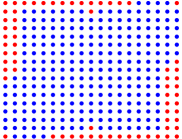
The discrete L2superscript𝐿2L^{2} HHD is carried out using 250250250 fixed measurements at random points in the domain 𝒟=[0,3π]2𝒟superscript03𝜋2\mathcal{D}=[0,3\pi]^{2}. We set the residual boundary energy εsubscript𝜀\varepsilon_{\partial\mathcal{I}} and ε𝒥subscript𝜀𝒥\varepsilon_{\partial\mathcal{J}} to 50%percent5050\% and the stopping criteria ΔεΔsubscript𝜀\Delta\varepsilon_{\partial\mathcal{I}} and Δε𝒥Δsubscript𝜀𝒥\Delta\varepsilon_{\partial\mathcal{J}} to 103superscript10310^{-3}. For the fractional Sobolev regularization, we selected ϵd=ϵc=104subscriptitalic-ϵdsubscriptitalic-ϵcsuperscript104\epsilon_{\mathrm{d}}=\epsilon_{\mathrm{c}}=10^{-4} and kd=kc=1.5subscript𝑘dsubscript𝑘c1.5k_{\mathrm{d}}=k_{\mathrm{c}}=1.5. After 151515 outer iterations, we obtained the index sets in Figure 1 with 149149149 (Figure 1A) and 103103103 (Figure 1B) entries for the divergence- and curl-free fields, respectively.
Refer to caption
(A) Index set: divergence-free field
Refer to caption
(B) Index set: curl-free field
Figure 1. Panels LABEL:sub@fg:ex5.div.index and LABEL:sub@fg:ex5.curl.index: Index sets of the reconstructed PiSL  divergence- and curl-free fields, respectively. Blue dots represent the indices retained in the Fourier construction. Red dots represent indices removed from the Fourier construction.

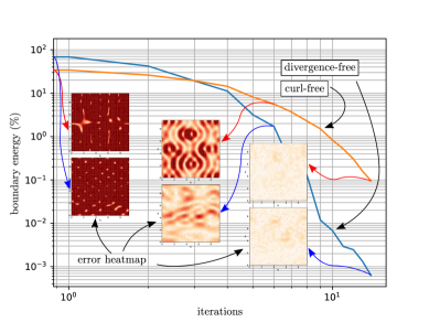
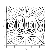
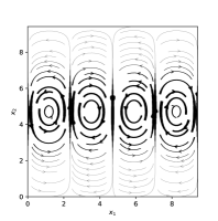
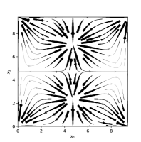
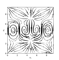
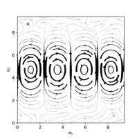
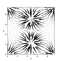
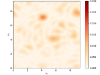
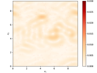
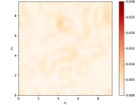
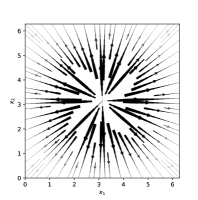
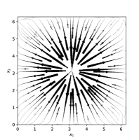
Table 1 presents the Lsuperscript𝐿L^{\infty} and L2superscript𝐿2L^{2} norms of the error e(𝒙)𝑒𝒙e(\boldsymbol{x}) for the total field 𝝊opt+𝝇𝒥optsuperscriptsubscript𝝊optsuperscriptsubscript𝝇𝒥opt\boldsymbol{\upsilon}_{\scriptscriptstyle\mathcal{I}}^{\mathrm{opt}}+\boldsymbol{\varsigma}_{\scriptscriptstyle\mathcal{J}}^{\mathrm{opt}}, divergence-free field 𝝊subscript𝝊\boldsymbol{\upsilon}_{\scriptscriptstyle\mathcal{I}}, and curl-free field 𝝇𝒥subscript𝝇𝒥\boldsymbol{\varsigma}_{\scriptscriptstyle\mathcal{J}}. As L(𝒖)1.16superscript𝐿norm𝒖1.16L^{\infty}(\|\boldsymbol{u}\|)\approx 1.16, the maximum relative error in any field is less than 2.0%percent2.02.0\%. This error is because we assume limited access to the data and can sample the data at a few fixed location points. This bias error vanishes if we allow the data to be sampled randomly at each optimization iteration. Figure 2 presents the convergence of the relative energy boundary along with error heatmaps for iterations 111, 888, and 141414 for both divergence- and curl-free errors. The blue curve depicts the convergence of the divergence-free reconstruction field, whereas the orange curve represents the convergence of the curl-free reconstruction field. The index sets increase with the iterations, these curves suggest that PiSL is endowed with spectral convergence. That is, for a constant q𝑞q, we obtain |𝝊𝜶|subscript𝝊𝜶|\boldsymbol{\upsilon}_{\boldsymbol{\alpha}}| and |𝝇𝜶|𝒪(e|𝜶|b)similar-tosubscript𝝇𝜶𝒪superscriptesuperscript𝜶𝑏|\boldsymbol{\varsigma}_{\boldsymbol{\alpha}}|\sim\mathcal{O}(\mathrm{e}^{-|\boldsymbol{\alpha}|^{b}}) where b𝑏b is the exponential index of convergence. For this problem, the exponential index of convergence is b20𝑏20b\approx-20. In Figure 3, from left to right in the first row, we present the underlying analytical fields: 𝒖𝒖\boldsymbol{u}, 𝒖csubscript𝒖c\boldsymbol{u}_{\mathrm{c}}, and 𝒖dsubscript𝒖d\boldsymbol{u}_{\mathrm{d}}. From left to right in the second row, we display the reconstructions: 𝝊+𝝇𝒥subscript𝝊subscript𝝇𝒥\boldsymbol{\upsilon}_{\scriptscriptstyle\mathcal{I}}+\boldsymbol{\varsigma}_{\scriptscriptstyle\mathcal{J}}, 𝝊subscript𝝊\boldsymbol{\upsilon}_{\scriptscriptstyle\mathcal{I}}, and 𝝇𝒥subscript𝝇𝒥\boldsymbol{\varsigma}_{\scriptscriptstyle\mathcal{J}}. From left to right in the third row, the reconstruction error corresponding to 𝝊+𝝇𝒥subscript𝝊subscript𝝇𝒥\boldsymbol{\upsilon}_{\scriptscriptstyle\mathcal{I}}+\boldsymbol{\varsigma}_{\scriptscriptstyle\mathcal{J}}, 𝝊subscript𝝊\boldsymbol{\upsilon}_{\scriptscriptstyle\mathcal{I}}, and 𝝇𝒥subscript𝝇𝒥\boldsymbol{\varsigma}_{\scriptscriptstyle\mathcal{J}} is in a scale from 00 to 0.030.030.03.

Table 1. Lsuperscript𝐿L^{\infty} and L2superscript𝐿2L^{2} norms of the error fields e𝑒e for the reconstructed total, curl-, and divergence-free fields.
e(𝒙)𝑒𝒙e(\boldsymbol{x}) L2(e(𝒙))superscript𝐿2𝑒𝒙L^{2}(e(\boldsymbol{x})) L(e(𝒙))superscript𝐿𝑒𝒙L^{\infty}(e(\boldsymbol{x}))
𝒖(𝒙)𝝊opt(𝒙)𝝇𝒥opt(𝒙)delimited-∥∥𝒖𝒙superscriptsubscript𝝊opt𝒙superscriptsubscript𝝇𝒥opt𝒙\left\lVert{\boldsymbol{u}(\boldsymbol{x})-\boldsymbol{\upsilon}_{\scriptscriptstyle\mathcal{I}}^{\mathrm{opt}}(\boldsymbol{x})-\boldsymbol{\varsigma}_{\scriptscriptstyle\mathcal{J}}^{\mathrm{opt}}(\boldsymbol{x})}\right\rVert 0.38840.38840.3884 0.023490.023490.02349
𝒖d(𝒙)𝝊opt(𝒙)delimited-∥∥subscript𝒖d𝒙superscriptsubscript𝝊opt𝒙\left\lVert{\boldsymbol{u}_{\mathrm{d}}(\boldsymbol{x})-\boldsymbol{\upsilon}_{\scriptscriptstyle\mathcal{I}}^{\mathrm{opt}}(\boldsymbol{x})}\right\rVert 0.33540.33540.3354 0.020080.020080.02008
𝒖c(𝒙)𝝇𝒥opt(𝒙)delimited-∥∥subscript𝒖c𝒙superscriptsubscript𝝇𝒥opt𝒙\left\lVert{\boldsymbol{u}_{\mathrm{c}}(\boldsymbol{x})-\boldsymbol{\varsigma}_{\scriptscriptstyle\mathcal{J}}^{\mathrm{opt}}(\boldsymbol{x})}\right\rVert 0.23760.23760.2376 0.016310.016310.01631
Refer to caption
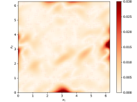
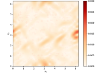
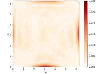
Figure 2. Convergence of the relative energy boundary along with error heatmaps for iterations 1, 8, and 14 for both divergence- and curl-free errors. Blue curve: divergence-free. Orange curve: curl-free.
Refer to caption
(A) Underlying field
Refer to caption
(B) Underlying div-free field
Refer to caption
(C) Underlying curl-free field
Refer to caption
(D) PiSL  field reconstruction
Refer to caption
(E) PiSL  div-free reconstruction
Refer to caption
(F) PiSL  curl-free reconstruction
Refer to caption
(G) Total error reconstruction
Refer to caption
(H) Div-free error
Refer to caption
(I) Curl-free error
Figure 3. Reconstructed PiSL  curl- and divergence-free fields. Panels LABEL:sub@fg:ex5.total.anal: 𝒖𝒖\boldsymbol{u} field, LABEL:sub@fg:ex5.div.anal: 𝒖dsubscript𝒖d\boldsymbol{u}_{\mathrm{d}} field, and LABEL:sub@fg:ex5.curl.anal: 𝒖csubscript𝒖c\boldsymbol{u}_{\mathrm{c}} field. Panels LABEL:sub@fg:ex5.total.PiSL: 𝝊+𝝇𝒥subscript𝝊subscript𝝇𝒥\boldsymbol{\upsilon}_{\scriptscriptstyle\mathcal{I}}+\boldsymbol{\varsigma}_{\scriptscriptstyle\mathcal{J}} field, LABEL:sub@fg:ex5.div.PiSL: 𝝊subscript𝝊\boldsymbol{\upsilon}_{\scriptscriptstyle\mathcal{I}} field, and LABEL:sub@fg:ex5.curl.PiSL: 𝝇𝒥subscript𝝇𝒥\boldsymbol{\varsigma}_{\scriptscriptstyle\mathcal{J}} field. Panels LABEL:sub@fg:ex5.total.err: error in the total field, LABEL:sub@fg:ex5.div.err: error in the divergence-free field, and LABEL:sub@fg:ex5.curl.err: error in the curl-free field.

4.2. Two-dimensional PiSL: vortices with a different scale and source

In the domain 𝒟=[D,D]𝒟𝐷𝐷\mathcal{D}=[D,D] with D=2π𝐷2𝜋D=2\pi, consider the underlying divergence-free field

(36) 𝒖d(𝒙)=12(cos(x1)sin(x2)+cos(2x1)sin(2x2),sin(x1)cos(x2)sin(2x1)cos(2x2)).subscript𝒖d𝒙12subscript𝑥1subscript𝑥22subscript𝑥12subscript𝑥2subscript𝑥1subscript𝑥22subscript𝑥12subscript𝑥2\boldsymbol{u}_{\mathrm{d}}(\boldsymbol{x})=\textstyle{\frac{{1}}{{2}}}(\cos(x_{1})\sin(x_{2})+\cos(2x_{1})\sin(2x_{2}),-\sin(x_{1})\cos(x_{2})-\sin(2x_{1})\cos(2x_{2})).

In addition, based on (31) and (32)2, consider the underlying curl-free field

(37) 𝒖c(𝒙)=𝝊c(𝒙;𝒙0),subscript𝒖c𝒙subscript𝝊c𝒙subscript𝒙0\boldsymbol{u}_{\mathrm{c}}(\boldsymbol{x})=-\boldsymbol{\upsilon}_{\mathrm{c}}(\boldsymbol{x};\boldsymbol{x}_{0}),

where 𝒙0=(D/2,D/2)subscript𝒙0𝐷2𝐷2\boldsymbol{x}_{0}=(D/2,D/2). Then, the field we aim to reconstruct while performing the discrete L2superscript𝐿2L^{2} HHD is given by

(38) 𝒖(𝒙)=𝒖d(𝒙)+𝒖c(𝒙).𝒖𝒙subscript𝒖d𝒙subscript𝒖c𝒙\boldsymbol{u}(\boldsymbol{x})=\boldsymbol{u}_{\mathrm{d}}(\boldsymbol{x})+\boldsymbol{u}_{\mathrm{c}}(\boldsymbol{x}).

The discrete L2superscript𝐿2L^{2} HHD is carried out using 250250250 fixed measurements at random points in the domain 𝒟=[0,2π]2𝒟superscript02𝜋2\mathcal{D}=[0,2\pi]^{2}. We set the residual boundary energy εsubscript𝜀\varepsilon_{\partial\mathcal{I}} and ε𝒥subscript𝜀𝒥\varepsilon_{\partial\mathcal{J}} to 50%percent5050\% and the stopping criteria ΔεΔsubscript𝜀\Delta\varepsilon_{\partial\mathcal{I}} and Δε𝒥Δsubscript𝜀𝒥\Delta\varepsilon_{\partial\mathcal{J}} to 103superscript10310^{-3}. For the fractional Sobolev regularization, we selected ϵd=ϵc=104subscriptitalic-ϵdsubscriptitalic-ϵcsuperscript104\epsilon_{\mathrm{d}}=\epsilon_{\mathrm{c}}=10^{-4} and kd=kc=1.5subscript𝑘dsubscript𝑘c1.5k_{\mathrm{d}}=k_{\mathrm{c}}=1.5. After 111111 outer iterations, we obtained the index sets in Figure 4 with 257257257 (Figure 4A) and 656565 (Figure 4B) entries for the divergence- and curl-free fields, respectively.

Refer to caption
(A) Index set: divergence-free field
Refer to caption
(B) Index set: curl-free field
Figure 4. Panels LABEL:sub@fg:ex6.div.index and LABEL:sub@fg:ex6.curl.index: Index sets of the reconstructed PiSL  divergence- and curl-free fields, respectively. Blue dots represent the indices retained in the Fourier construction. Red dots represent indices removed from the Fourier construction.

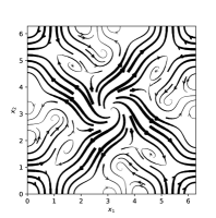
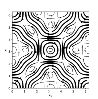
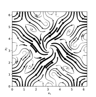
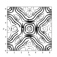
Table 2 lists the Lsuperscript𝐿L^{\infty} and L2superscript𝐿2L^{2} norms of the error e(𝒙)𝑒𝒙e(\boldsymbol{x}) for the total field 𝝊opt+𝝇𝒥optsuperscriptsubscript𝝊optsuperscriptsubscript𝝇𝒥opt\boldsymbol{\upsilon}_{\scriptscriptstyle\mathcal{I}}^{\mathrm{opt}}+\boldsymbol{\varsigma}_{\scriptscriptstyle\mathcal{J}}^{\mathrm{opt}}, divergence-free field 𝝊subscript𝝊\boldsymbol{\upsilon}_{\scriptscriptstyle\mathcal{I}}, and curl-free field 𝝇𝒥subscript𝝇𝒥\boldsymbol{\varsigma}_{\scriptscriptstyle\mathcal{J}}. As L(𝒖)0.97superscript𝐿norm𝒖0.97L^{\infty}(\|\boldsymbol{u}\|)\approx 0.97, the maximum relative error in any field is less than 2.5%percent2.52.5\%. In Figure 5, from left to right in the first row, we present the underlying analytical fields: 𝒖𝒖\boldsymbol{u}, 𝒖csubscript𝒖c\boldsymbol{u}_{\mathrm{c}}, and 𝒖dsubscript𝒖d\boldsymbol{u}_{\mathrm{d}}. From left to right in the second row, we display the reconstructions: 𝝊+𝝇𝒥subscript𝝊subscript𝝇𝒥\boldsymbol{\upsilon}_{\scriptscriptstyle\mathcal{I}}+\boldsymbol{\varsigma}_{\scriptscriptstyle\mathcal{J}}, 𝝊subscript𝝊\boldsymbol{\upsilon}_{\scriptscriptstyle\mathcal{I}}, and 𝝇𝒥subscript𝝇𝒥\boldsymbol{\varsigma}_{\scriptscriptstyle\mathcal{J}}. From left to right in the third row, the reconstruction error corresponding to 𝝊+𝝇𝒥subscript𝝊subscript𝝇𝒥\boldsymbol{\upsilon}_{\scriptscriptstyle\mathcal{I}}+\boldsymbol{\varsigma}_{\scriptscriptstyle\mathcal{J}}, 𝝊subscript𝝊\boldsymbol{\upsilon}_{\scriptscriptstyle\mathcal{I}}, and 𝝇𝒥subscript𝝇𝒥\boldsymbol{\varsigma}_{\scriptscriptstyle\mathcal{J}} is in a scale from 00 to 0.030.030.03.

Table 2. Lsuperscript𝐿L^{\infty} and L2superscript𝐿2L^{2} norms of the error fields e𝑒e for the reconstructed total, curl-, and divergence-free fields.
e(𝒙)𝑒𝒙e(\boldsymbol{x}) L2(e(𝒙))superscript𝐿2𝑒𝒙L^{2}(e(\boldsymbol{x})) L(e(𝒙))superscript𝐿𝑒𝒙L^{\infty}(e(\boldsymbol{x}))
𝒖(𝒙)𝝊opt(𝒙)𝝇𝒥opt(𝒙)delimited-∥∥𝒖𝒙superscriptsubscript𝝊opt𝒙superscriptsubscript𝝇𝒥opt𝒙\left\lVert{\boldsymbol{u}(\boldsymbol{x})-\boldsymbol{\upsilon}_{\scriptscriptstyle\mathcal{I}}^{\mathrm{opt}}(\boldsymbol{x})-\boldsymbol{\varsigma}_{\scriptscriptstyle\mathcal{J}}^{\mathrm{opt}}(\boldsymbol{x})}\right\rVert 0.99430.99430.9943 0.025190.025190.02519
𝒖d(𝒙)𝝊opt(𝒙)delimited-∥∥subscript𝒖d𝒙superscriptsubscript𝝊opt𝒙\left\lVert{\boldsymbol{u}_{\mathrm{d}}(\boldsymbol{x})-\boldsymbol{\upsilon}_{\scriptscriptstyle\mathcal{I}}^{\mathrm{opt}}(\boldsymbol{x})}\right\rVert 0.40180.40180.4018 0.017650.017650.01765
𝒖c(𝒙)𝝇𝒥opt(𝒙)delimited-∥∥subscript𝒖c𝒙superscriptsubscript𝝇𝒥opt𝒙\left\lVert{\boldsymbol{u}_{\mathrm{c}}(\boldsymbol{x})-\boldsymbol{\varsigma}_{\scriptscriptstyle\mathcal{J}}^{\mathrm{opt}}(\boldsymbol{x})}\right\rVert 0.95660.95660.9566 0.020100.020100.02010
Refer to caption
(A) Underlying field
Refer to caption
(B) Underlying div-free field
Refer to caption
(C) Underlying curl-free field
Refer to caption
(D) PiSL  field reconstruction
Refer to caption
(E) PiSL  div-free reconstruction
Refer to caption
(F) PiSL  curl-free reconstruction
Refer to caption
(G) Total error reconstruction
Refer to caption
(H) Div-free error
Refer to caption
(I) Curl-free error
Figure 5. Reconstructed PiSL  curl- and divergence-free fields. Panels LABEL:sub@fg:ex6.total.anal: 𝒖𝒖\boldsymbol{u} field, LABEL:sub@fg:ex6.div.anal: 𝒖dsubscript𝒖d\boldsymbol{u}_{\mathrm{d}} field, and LABEL:sub@fg:ex6.curl.anal: 𝒖csubscript𝒖c\boldsymbol{u}_{\mathrm{c}} field. Panels LABEL:sub@fg:ex6.total.PiSL: 𝝊+𝝇𝒥subscript𝝊subscript𝝇𝒥\boldsymbol{\upsilon}_{\scriptscriptstyle\mathcal{I}}+\boldsymbol{\varsigma}_{\scriptscriptstyle\mathcal{J}} field, LABEL:sub@fg:ex6.div.PiSL: 𝝊subscript𝝊\boldsymbol{\upsilon}_{\scriptscriptstyle\mathcal{I}} field, and LABEL:sub@fg:ex6.curl.PiSL: 𝝇𝒥subscript𝝇𝒥\boldsymbol{\varsigma}_{\scriptscriptstyle\mathcal{J}} field. Panels LABEL:sub@fg:ex6.total.err: error in the total field, LABEL:sub@fg:ex6.div.err: error in the divergence-free field, and LABEL:sub@fg:ex6.curl.err: error in the curl-free field.

4.3. Three-dimensional PiSL: vortices with a different scale and source

This example is a three-dimensional extension of the previous example with a domain 𝒟=[D,D,D]𝒟𝐷𝐷𝐷\mathcal{D}=[D,D,D] with D=2π𝐷2𝜋D=2\pi. The underlying divergence-free field is given by

𝒖d(𝒙)=subscript𝒖d𝒙absent\displaystyle\boldsymbol{u}_{\mathrm{d}}(\boldsymbol{x})={} (12(cos(x1)sin(x2)cos(x3)+cos(2x1)sin(2x2)cos(x3)),\displaystyle(\textstyle{\frac{{1}}{{2}}}(\cos(x_{1})\sin(x_{2})\cos(x_{3})+\cos(2x_{1})\sin(2x_{2})\cos(x_{3})),
12(sin(x1)cos(x2)cos(x3)sin(2x1)cos(2x2)cos(2x3)),12subscript𝑥1subscript𝑥2subscript𝑥32subscript𝑥12subscript𝑥22subscript𝑥3\displaystyle\textstyle{\frac{{1}}{{2}}}(-\sin(x_{1})\cos(x_{2})\cos(x_{3})-\sin(2x_{1})\cos(2x_{2})\cos(2x_{3})),
12(sin(x1)sin(x2)(sin(x3)12sin(2x3))+2sin(2x1)sin(2x2)(sin(x3)\displaystyle\textstyle{\frac{{1}}{{2}}}(\sin(x_{1})\sin(x_{2})(\sin(x_{3})-\textstyle{\frac{{1}}{{2}}}\sin(2x_{3}))+2\sin(2x_{1})\sin(2x_{2})(\sin(x_{3})
(39) 12sin(2x3)))(12sin(x3)14sin(2x3))sin(x1)sin(x2)]),\displaystyle-\textstyle{\frac{{1}}{{2}}}\sin(2x_{3})))-(\textstyle{\frac{{1}}{{2}}}\sin(x_{3})-\textstyle{\frac{{1}}{{4}}}\sin(2x_{3}))\sin(x_{1})\sin(x_{2})]),

whereas, based on (31) and (32)2, the curl-free field is

(40) 𝒖c(𝒙)=𝝊c(𝒙;𝒙0),subscript𝒖c𝒙subscript𝝊c𝒙subscript𝒙0\boldsymbol{u}_{\mathrm{c}}(\boldsymbol{x})=-\boldsymbol{\upsilon}_{\mathrm{c}}(\boldsymbol{x};\boldsymbol{x}_{0}),

where 𝒙0=(D/2,D/2,D/2)subscript𝒙0𝐷2𝐷2𝐷2\boldsymbol{x}_{0}=(D/2,D/2,D/2). Thus, the field we aim to reconstruct while performing the discrete L2superscript𝐿2L^{2} HHD is given by

(41) 𝒖(𝒙)=𝒖d(𝒙)+𝒖c(𝒙).𝒖𝒙subscript𝒖d𝒙subscript𝒖c𝒙\boldsymbol{u}(\boldsymbol{x})=\boldsymbol{u}_{\mathrm{d}}(\boldsymbol{x})+\boldsymbol{u}_{\mathrm{c}}(\boldsymbol{x}).

The discrete L2superscript𝐿2L^{2} HHD is carried out using 102410241024 fixed measurements at random points in the domain 𝒟=[0,2π]3𝒟superscript02𝜋3\mathcal{D}=[0,2\pi]^{3}. We set the residual boundary energies εsubscript𝜀\varepsilon_{\partial\mathcal{I}} and ε𝒥subscript𝜀𝒥\varepsilon_{\partial\mathcal{J}} to 20%percent2020\% and the stopping criteria ΔεΔsubscript𝜀\Delta\varepsilon_{\partial\mathcal{I}} and Δε𝒥Δsubscript𝜀𝒥\Delta\varepsilon_{\partial\mathcal{J}} to 103superscript10310^{-3}. For the fractional Sobolev regularization, we selected ϵd=ϵc=106subscriptitalic-ϵdsubscriptitalic-ϵcsuperscript106\epsilon_{\mathrm{d}}=\epsilon_{\mathrm{c}}=10^{-6} and kd=kc=1.6subscript𝑘dsubscript𝑘c1.6k_{\mathrm{d}}=k_{\mathrm{c}}=1.6. After 555 outer iterations, we obtained the index sets in Figure 6 with 583583583 (Figure 4A) and 477477477 (Figure 4B) entries for the divergence- and curl-free fields, respectively.

Refer to caption
(A) (4,:,:)4::\mathcal{I}(-4,:,:)
Refer to caption
(B) (3,:,:)3::\mathcal{I}(-3,:,:)
Refer to caption
(C) (2,:,:)2::\mathcal{I}(-2,:,:)
Refer to caption
(D) (1,:,:)1::\mathcal{I}(-1,:,:)
Refer to caption
(E) (0,:,:)0::\mathcal{I}(0,:,:)
Refer to caption
(F) (1,:,:)1::\mathcal{I}(1,:,:)
Refer to caption
(G) (2,:,:)2::\mathcal{I}(2,:,:)
Refer to caption
(H) (3,:,:)3::\mathcal{I}(3,:,:)
Refer to caption
(I) (4,:,:)4::\mathcal{I}(4,:,:)
Figure 6. Index set: divergence-free field. Panels LABEL:sub@fg:index.div.1, LABEL:sub@fg:index.div.2, LABEL:sub@fg:index.div.3, LABEL:sub@fg:index.div.4, LABEL:sub@fg:index.div.5, LABEL:sub@fg:index.div.6, LABEL:sub@fg:index.div.7, LABEL:sub@fg:index.div.8, and LABEL:sub@fg:index.div.9: (4,:,:)4::\mathcal{I}(-4,:,:), (3,:,:)3::\mathcal{I}(-3,:,:), (2,:,:)2::\mathcal{I}(-2,:,:), (1,:,:)1::\mathcal{I}(-1,:,:), (0,:,:)0::\mathcal{I}(0,:,:), (1,:,:)1::\mathcal{I}(1,:,:), (2,:,:)2::\mathcal{I}(2,:,:), (3,:,:)3::\mathcal{I}(3,:,:), and (4,:,:)4::\mathcal{I}(4,:,:), respectively. Blue dots represent the indices retained in the Fourier construction. Red dots represent indices removed from the Fourier construction.
Refer to caption
(A) 𝒥(4,:,:)𝒥4::\mathcal{J}(-4,:,:)
Refer to caption
(B) 𝒥(3,:,:)𝒥3::\mathcal{J}(-3,:,:)
Refer to caption
(C) 𝒥(2,:,:)𝒥2::\mathcal{J}(-2,:,:)
Refer to caption
(D) 𝒥(1,:,:)𝒥1::\mathcal{J}(-1,:,:)
Refer to caption
(E) 𝒥(0,:,:)𝒥0::\mathcal{J}(0,:,:)
Refer to caption
(F) 𝒥(1,:,:)𝒥1::\mathcal{J}(1,:,:)
Refer to caption
(G) 𝒥(2,:,:)𝒥2::\mathcal{J}(2,:,:)
Refer to caption
(H) 𝒥(3,:,:)𝒥3::\mathcal{J}(3,:,:)
Refer to caption
(I) 𝒥(4,:,:)𝒥4::\mathcal{J}(4,:,:)
Figure 7. Index set: curl-free field. Panels LABEL:sub@fg:index.curl.1, LABEL:sub@fg:index.curl.2, LABEL:sub@fg:index.curl.3, LABEL:sub@fg:index.curl.4, LABEL:sub@fg:index.curl.5, LABEL:sub@fg:index.curl.6, LABEL:sub@fg:index.curl.7, LABEL:sub@fg:index.curl.8, and LABEL:sub@fg:index.curl.9: 𝒥(4,:,:)𝒥4::\mathcal{J}(-4,:,:), 𝒥(3,:,:)𝒥3::\mathcal{J}(-3,:,:), 𝒥(2,:,:)𝒥2::\mathcal{J}(-2,:,:), 𝒥(1,:,:)𝒥1::\mathcal{J}(-1,:,:), 𝒥(0,:,:)𝒥0::\mathcal{J}(0,:,:), 𝒥(1,:,:)𝒥1::\mathcal{J}(1,:,:), 𝒥(2,:,:)𝒥2::\mathcal{J}(2,:,:), 𝒥(3,:,:)𝒥3::\mathcal{J}(3,:,:), and 𝒥(4,:,:)𝒥4::\mathcal{J}(4,:,:), respectively. Blue dots represent the indices retained in the Fourier construction. Red dots represent indices removed from the Fourier construction.

Table 3 presents the Lsuperscript𝐿L^{\infty} and L2superscript𝐿2L^{2} norms of the error e(𝒙)𝑒𝒙e(\boldsymbol{x}) for the total 𝝊opt+𝝇𝒥optsuperscriptsubscript𝝊optsuperscriptsubscript𝝇𝒥opt\boldsymbol{\upsilon}_{\scriptscriptstyle\mathcal{I}}^{\mathrm{opt}}+\boldsymbol{\varsigma}_{\scriptscriptstyle\mathcal{J}}^{\mathrm{opt}}, divergence-free 𝝊subscript𝝊\boldsymbol{\upsilon}_{\scriptscriptstyle\mathcal{I}}, and curl-free 𝝇𝒥subscript𝝇𝒥\boldsymbol{\varsigma}_{\scriptscriptstyle\mathcal{J}} fields. As L(𝒖)1.7superscript𝐿norm𝒖1.7L^{\infty}(\|\boldsymbol{u}\|)\approx 1.7, the maximum relative error in any field is less than 2.0%percent2.02.0\%. In Figure 8, we present the magnitude of reconstructions from left to right: 𝝊+𝝇𝒥subscript𝝊subscript𝝇𝒥\boldsymbol{\upsilon}_{\scriptscriptstyle\mathcal{I}}+\boldsymbol{\varsigma}_{\scriptscriptstyle\mathcal{J}}, 𝝊subscript𝝊\boldsymbol{\upsilon}_{\scriptscriptstyle\mathcal{I}}, and 𝝇𝒥subscript𝝇𝒥\boldsymbol{\varsigma}_{\scriptscriptstyle\mathcal{J}}. Figure 9 provides the reconstruction errors from left to right, corresponding to 𝝊+𝝇𝒥subscript𝝊subscript𝝇𝒥\boldsymbol{\upsilon}_{\scriptscriptstyle\mathcal{I}}+\boldsymbol{\varsigma}_{\scriptscriptstyle\mathcal{J}}, 𝝊subscript𝝊\boldsymbol{\upsilon}_{\scriptscriptstyle\mathcal{I}}, and 𝝇𝒥subscript𝝇𝒥\boldsymbol{\varsigma}_{\scriptscriptstyle\mathcal{J}} on a scale from 00 to 0.030.030.03.

Table 3. Lsuperscript𝐿L^{\infty} and L2superscript𝐿2L^{2} norms of the error fields e𝑒e for the reconstructed total, curl-, and divergence-free fields.
e(𝒙)𝑒𝒙e(\boldsymbol{x}) L2(e(𝒙))superscript𝐿2𝑒𝒙L^{2}(e(\boldsymbol{x})) L(e(𝒙))superscript𝐿𝑒𝒙L^{\infty}(e(\boldsymbol{x}))
𝒖(𝒙)𝝊opt(𝒙)𝝇𝒥opt(𝒙)delimited-∥∥𝒖𝒙superscriptsubscript𝝊opt𝒙superscriptsubscript𝝇𝒥opt𝒙\left\lVert{\boldsymbol{u}(\boldsymbol{x})-\boldsymbol{\upsilon}_{\scriptscriptstyle\mathcal{I}}^{\mathrm{opt}}(\boldsymbol{x})-\boldsymbol{\varsigma}_{\scriptscriptstyle\mathcal{J}}^{\mathrm{opt}}(\boldsymbol{x})}\right\rVert 0.37420.37420.3742 0.032000.032000.03200
𝒖d(𝒙)𝝊opt(𝒙)delimited-∥∥subscript𝒖d𝒙superscriptsubscript𝝊opt𝒙\left\lVert{\boldsymbol{u}_{\mathrm{d}}(\boldsymbol{x})-\boldsymbol{\upsilon}_{\scriptscriptstyle\mathcal{I}}^{\mathrm{opt}}(\boldsymbol{x})}\right\rVert 0.24750.24750.2475 0.011260.011260.01126
𝒖d(𝒙)𝝊opt(𝒙)delimited-∥∥subscript𝒖d𝒙superscriptsubscript𝝊opt𝒙\left\lVert{\boldsymbol{u}_{\mathrm{d}}(\boldsymbol{x})-\boldsymbol{\upsilon}_{\scriptscriptstyle\mathcal{I}}^{\mathrm{opt}}(\boldsymbol{x})}\right\rVert 0.32580.32580.3258 0.025740.025740.02574
Refer to caption
(A) PiSL  field reconstruction
Refer to caption
(B) PiSL  div-free reconstruction
Refer to caption
(C) PiSL  curl-free reconstruction
Figure 8. Reconstructed PiSL  curl- and divergence-free fields. Panels LABEL:sub@fg:3d.div.curl: 𝝊+𝝇𝒥subscript𝝊subscript𝝇𝒥\boldsymbol{\upsilon}_{\scriptscriptstyle\mathcal{I}}+\boldsymbol{\varsigma}_{\scriptscriptstyle\mathcal{J}} field, LABEL:sub@fg:3d.div: 𝝊subscript𝝊\boldsymbol{\upsilon}_{\scriptscriptstyle\mathcal{I}} field, and LABEL:sub@fg:3d.curl: 𝝇𝒥subscript𝝇𝒥\boldsymbol{\varsigma}_{\scriptscriptstyle\mathcal{J}} field.
Refer to caption
(A) PiSL  field L(e)=3.2e2superscript𝐿𝑒3.2𝑒2L^{\infty}(e)=3.2e-2
Refer to caption
(B) PiSL  div-free field L(e)=1.1e2superscript𝐿𝑒1.1𝑒2L^{\infty}(e)=1.1e-2
Refer to caption
(C) PiSL  curl-free field L(e)=2.6e2superscript𝐿𝑒2.6𝑒2L^{\infty}(e)=2.6e-2
Figure 9. Reconstructed PiSL  curl- and divergence-free fields. Panels LABEL:sub@fg:3d.div.curl.err: error in the total field, LABEL:sub@fg:3d.div.err: error in the divergence-free field, and LABEL:sub@fg:3d.curl.err: error in the curl-free field.

4.4. ‘The storm of the century’

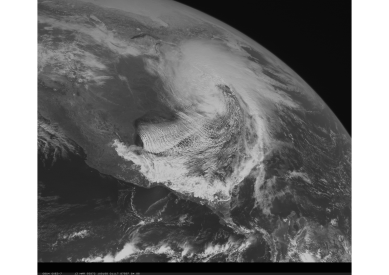
The Storm of the Century (also known as the 93 Superstorm, No Name Storm, or Great Blizzard of 1993) occurred from March 12 to 14 in 1993. It was a large cyclonic storm that formed over the Gulf of Mexico. The intensity, massive size, and wide-reaching effects made the storm unique. The storm stretched from Canada to Honduras [9]. Moreover, the storm is one the most significant storms to affect the eastern United States. On March 13, a larger-scale view of Meteosat-3 infrared (11.511.511.5 μ𝜇\mum) images (Figure 10) revealed the vast size of the storm as it moved along the Eastern Seaboard of the US. Some highlights of the storm included snowfall amounts as high as 56 inches at Mount LeConte in Tennessee, wind gusts of 144144144 mph in Mount Washington in New Hampshire, a minimum sea level pressure of 28.2828.2828.28 inches in White Plains in New York, and a post-storm record low temperature of 24.424.4-24.4℃  in Burlington, Vermont [10].

Refer to caption
Figure 10. March 12–14, 1993 ‘Storm of the Century’ (also known as the 93 Superstorm, No Name Storm, or Great Blizzard of 1993). Picture made available by CIMSS Satellite Blog https://www.ssec.wisc.edu/mcidas/images/goes7_vis_19930313_storm_of_century.jpg.

Fed by real satellite data, we employ our HHD PiSL  framework for hurricane tracking. Therefore, we aim to identify the center of rotation, namely the hurricane eye in the storm of the century, see Figure 10. However, the main difficulty arising when dealing with real data is corrupted data. Measurements errors are intrinsic to real data. Therefore, one must avoid overfitting. In the PiSL  framework, we control the energy of the higher Fourier modes to assess the quality of the reconstruction and use it as a stopping criterion (see Espath et al. [1]). In this example instead, we limit the energy boundary to 111% and 5%percent55\%, for the divergence- and curl-free components, respectively, of the total energy of the approximated solution. This means that we avoid overfitting by not approximating the high freaquences corresponding to 111% and 5%percent55\%, for the divergence- and curl-free components, respectively, of the total energy.

The discrete L2superscript𝐿2L^{2} HHD is carried out using approximately 650650650 fixed measurements. We set the residual boundary energy εsubscript𝜀\varepsilon_{\partial\mathcal{I}} and ε𝒥subscript𝜀𝒥\varepsilon_{\partial\mathcal{J}} to 50%percent5050\% and the stopping criteria ΔεΔsubscript𝜀\Delta\varepsilon_{\partial\mathcal{I}} and Δε𝒥Δsubscript𝜀𝒥\Delta\varepsilon_{\partial\mathcal{J}} to 102superscript10210^{-2} and 5×1025superscript1025\times 10^{-2}, respectively. For the fractional Sobolev regularization, we selected ϵd=ϵc=103subscriptitalic-ϵdsubscriptitalic-ϵcsuperscript103\epsilon_{\mathrm{d}}=\epsilon_{\mathrm{c}}=10^{-3} and kd=kc=1.5subscript𝑘dsubscript𝑘c1.5k_{\mathrm{d}}=k_{\mathrm{c}}=1.5. After 999 outer iterations, we obtained the index sets in Figure 11A with 777777 (Figure 1A) and 636363 (Figure 11B) entries for the divergence- and curl-free fields, respectively.

Refer to caption
(A) Index set: divergence-free field
Refer to caption
(B) Index set: curl-free field
Figure 11. Panels LABEL:sub@fg:1993.div.index and LABEL:sub@fg:1993.curl.index: Index sets of the reconstructed PiSL  divergence- and curl-free fields, respectively. Blue dots represent the indices kept in the Fourier construction. Red dots represent indices removed from the Fourier construction.

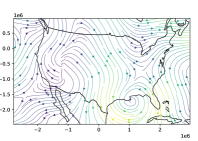
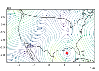
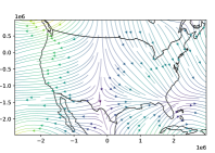
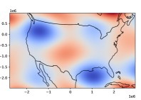
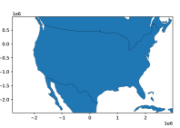
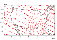
In Figure 12, we depict the identification of the hurricane eye in the storm of the century in 1993. Figures 12A and 12B present the map and the satellite data used in this discrete HHD PiSL  problem, respectively. Figures 12D show the PiSL  divergence-free reconstructed component with the red dot indicating the hurricane eye, whereas Figure 12E presents the PiSL  curl-free reconstructed component. Figure 12C presents the reconstructed PiSL  field and Figure 12F presents the PiSL  vorticity field. Figure 12C reveals two main vortical structures, whereas only one vortex is identified in the divergence-free reconstructed component, corresponding to the hurricane eye. The additional ‘vortex’ is an artifact of the two-dimensional data because the satellite preprocess data do not capture the vertical component of the wind velocity. Lastly, in Figure 12F, we present the vorticity of the reconstructed velocity field.
Refer to caption
(A) Map
Refer to caption
(B) Satellite data
Refer to caption
(C) PiSL  wind field reconstrution
Refer to caption
(D) PiSL  div-free field reconstruction (red dot indicates the hurricane eye)
Refer to caption
(E) PiSL  curl-free field reconstruction
Refer to caption
(F) PiSL  vorticity field reconstruction
Figure 12. Panels LABEL:sub@fg:1993.map: map, LABEL:sub@fg:1993.data: satellite data, LABEL:sub@fg:1993.reconstruction: PiSL  field reconstruction, LABEL:sub@fg:1993.div: PiSL  divergence-free field (red dot indicates the hurricane eye), LABEL:sub@fg:1993.curl: PiSL  curl-free field, and LABEL:sub@fg:1993.vorticity: PiSL  vorticity field. Data from the National Center for Environmental Information (NCEI, formerly NCDC) on a THREDDS server. https://www.ncei.noaa.gov/thredds/catalog/model-narr-a-files/199303/19930313/catalog.html?dataset=model-narr-a-files/199303/19930313/narr-a_221_19930313_0000_000.grb)

5. Conclusions

We further develop the Physics-informed Spectral Learning (PiSL) method introduced by Espath et al. [1] based on a discrete L2superscript𝐿2L^{2} projection to solve the discrete Helmholtz–Hodge decomposition. In this adaptive physical-informed type of statistical learning framework, we adaptively build a sparse Fourier set of basis functions and their coefficients by solving a sequence of minimization problems. The sparse Fourier set of basis functions is augmented greedily in each optimization problem. We regularize our minimization problems with the seminorm of the fractional Sobolev space in a Tikhonov fashion. PiSL  method ejoys spectral (exponential) convergence and is powerful enough to reconstruct vector fields from even very sparse data. The reconstruction and identification of the hurricane eye in the storm of the century also depicts the robustness of the discrete L2superscript𝐿2L^{2} HHD using PiSL.

6. Acknowledgments

This work was partially supported by the Flexible Interdisciplinary Research Collaboration Fund at the University of Nottingham Project ID 7466664. This work was partially supported by the KAUST Office of Sponsored Research (OSR) under Award numbers URF/1/22810101absent122810101/1/2281-01-01, URF/1/25840101absent125840101/1/2584-01-01 in the KAUST Competitive Research Grants Program Round 8.

Last but not least, we want to thank Prof. Jesper Oppelstrup for providing us with valuable ideas and constructive comments.

7. Conflict of interest

The authors have no conflicts to disclose.

8. Data Availability

The data that support the findings of this study are available from the corresponding author upon reasonable request.

Appendix A Inner product

Recalling that

(A.42) 𝜶^=(α1/D1,,αn/Dn)with𝜶n,formulae-sequence^𝜶subscript𝛼1subscript𝐷1subscript𝛼𝑛subscript𝐷𝑛with𝜶superscript𝑛\hat{\boldsymbol{\alpha}}=(\alpha_{1}/D_{1},\ldots,\alpha_{n}/D_{n})\qquad\text{with}\qquad\boldsymbol{\alpha}\in\mathbb{Z}^{n},

consider

(A.43) 𝝃𝒜(𝒙)𝜶𝒜𝝊𝜶φ(𝒙,𝜶)and𝜻(𝒙)𝜶𝝇𝜶φ(𝒙,𝜶),formulae-sequencesubscript𝝃𝒜𝒙subscript𝜶𝒜subscript𝝊𝜶𝜑𝒙𝜶andsubscript𝜻𝒙subscript𝜶subscript𝝇𝜶𝜑𝒙𝜶\displaystyle\boldsymbol{\xi}_{\scriptscriptstyle\mathcal{A}}(\boldsymbol{x})\coloneqq\sum\limits_{\boldsymbol{\alpha}\in\mathcal{A}}\boldsymbol{\upsilon}_{\boldsymbol{\alpha}}\varphi(\boldsymbol{x},\boldsymbol{\alpha})\qquad\text{and}\qquad\boldsymbol{\zeta}_{\scriptscriptstyle\mathcal{B}}(\boldsymbol{x})\coloneqq\sum\limits_{\boldsymbol{\alpha}\in\mathcal{B}}\boldsymbol{\varsigma}_{\boldsymbol{\alpha}}\varphi(\boldsymbol{x},\boldsymbol{\alpha}),
withφ(𝒙,𝜶)exp(2πȷ𝜶^𝒙)𝒙Πβ=1n[0,Dβ]𝜶𝒜,,formulae-sequencewith𝜑𝒙𝜶2𝜋italic-ȷ^𝜶𝒙for-all𝒙superscriptsubscriptΠ𝛽1𝑛0subscript𝐷𝛽𝜶𝒜\displaystyle\text{with}\qquad\varphi(\boldsymbol{x},\boldsymbol{\alpha})\coloneqq\exp(2\pi\jmath\,\hat{\boldsymbol{\alpha}}\cdot\boldsymbol{x})\qquad\forall\,\boldsymbol{x}\in\Pi_{\beta=1}^{n}[0,D_{\beta}]\wedge\boldsymbol{\alpha}\in\mathcal{A},\mathcal{B},

where 𝒜𝒜\mathcal{A} and nsuperscript𝑛\mathcal{B}\subset\mathbb{Z}^{n} are finite index sets of tuples composed of n𝑛n integers defining the indices of the basis functions and 𝝊𝜶,𝝇𝜶nsubscript𝝊𝜶subscript𝝇𝜶superscript𝑛\boldsymbol{\upsilon}_{\boldsymbol{\alpha}},\,\boldsymbol{\varsigma}_{\boldsymbol{\alpha}}\,\in\mathbb{C}^{n} are their Fourier coefficients, for all 𝜶𝒜𝜶𝒜\boldsymbol{\alpha}\in\mathcal{A} and 𝜶𝜶\boldsymbol{\alpha}\in\mathcal{B}, respectively.

With the L2superscript𝐿2L^{2} inner product

(A.44) (𝝃𝒜,𝜻)L2(𝒟)1|𝒟|𝒟𝝃𝒜𝜻dv,subscriptsubscript𝝃𝒜subscript𝜻superscript𝐿2𝒟1𝒟subscript𝒟subscript𝝃𝒜superscriptsubscript𝜻differential-d𝑣(\boldsymbol{\xi}_{\scriptscriptstyle\mathcal{A}},\boldsymbol{\zeta}_{\scriptscriptstyle\mathcal{B}})_{L^{2}(\mathcal{D})}\coloneqq\dfrac{1}{|\mathcal{D}|}\int_{\mathcal{D}}\boldsymbol{\xi}_{\scriptscriptstyle\mathcal{A}}\cdot\boldsymbol{\zeta}_{\scriptscriptstyle\mathcal{B}}^{\ast}\,\mathrm{d}v,

and as the bases are orthogonal, that is,

(A.45) (φ(𝒙,𝜶),φ(𝒙,𝜷))L2(𝒟)={0if𝜶𝜷,1if𝜶=𝜷.subscript𝜑𝒙𝜶superscript𝜑𝒙𝜷superscript𝐿2𝒟cases0if𝜶𝜷1if𝜶𝜷(\varphi(\boldsymbol{x},\boldsymbol{\alpha}),\varphi^{\ast}(\boldsymbol{x},\boldsymbol{\beta}))_{L^{2}(\mathcal{D})}=\begin{cases}0&\text{if}\,\boldsymbol{\alpha}\neq\boldsymbol{\beta},\\[4.0pt] 1&\text{if}\,\boldsymbol{\alpha}=\boldsymbol{\beta}.\end{cases}

for k𝑘k\in\mathbb{R}, and recalling that

(A.46) gradφ(𝒙,𝜶)=2πȷφ(𝒙,𝜶)𝜶^,grad𝜑𝒙𝜶2𝜋italic-ȷ𝜑𝒙𝜶^𝜶\mathrm{grad}\mskip 2.0mu\varphi(\boldsymbol{x},\boldsymbol{\alpha})=2\pi\jmath\mskip 3.0mu\varphi(\boldsymbol{x},\boldsymbol{\alpha})\mskip 3.0mu\hat{\boldsymbol{\alpha}},

the L2superscript𝐿2L^{2} inner product between the fractional k𝑘kth gradients of 𝝃𝒜subscript𝝃𝒜\boldsymbol{\xi}_{\scriptscriptstyle\mathcal{A}} and 𝜻subscript𝜻\boldsymbol{\zeta}_{\scriptscriptstyle\mathcal{B}} is given by

(𝝃𝒜,𝜻)H̊k(𝒟)subscriptsubscript𝝃𝒜subscript𝜻superscript̊𝐻𝑘𝒟\displaystyle(\boldsymbol{\xi}_{\scriptscriptstyle\mathcal{A}},\boldsymbol{\zeta}_{\scriptscriptstyle\mathcal{B}})_{\mathring{H}^{k}(\mathcal{D})} =1|𝒟|𝒟gradk𝝃𝒜:(gradk𝜻)dv:absent1𝒟subscript𝒟superscriptgrad𝑘subscript𝝃𝒜superscriptsuperscriptgrad𝑘subscript𝜻d𝑣\displaystyle=\dfrac{1}{|\mathcal{D}|}\int_{\mathcal{D}}\mathrm{grad}\mskip 2.0mu^{k}\boldsymbol{\xi}_{\scriptscriptstyle\mathcal{A}}\mskip 2.0mu\colon\mskip-2.0mu(\mathrm{grad}\mskip 2.0mu^{k}\boldsymbol{\zeta}_{\scriptscriptstyle\mathcal{B}})^{\ast}\,\mathrm{d}v
=1|𝒟|𝒟(𝜶𝒜𝝃𝜶gradkφ(𝒙,𝜶)):(𝜷𝜻𝜷gradkφ(𝒙,𝜷))dv,:absent1𝒟subscript𝒟subscript𝜶𝒜tensor-productsubscript𝝃𝜶superscriptgrad𝑘𝜑𝒙𝜶subscript𝜷tensor-productsuperscriptsubscript𝜻𝜷superscriptgrad𝑘superscript𝜑𝒙𝜷d𝑣\displaystyle=\dfrac{1}{|\mathcal{D}|}\int_{\mathcal{D}}\Bigg{(}\sum\limits_{\boldsymbol{\alpha}\in\mathcal{A}}\boldsymbol{\xi}_{\boldsymbol{\alpha}}\otimes\mathrm{grad}\mskip 2.0mu^{k}\varphi(\boldsymbol{x},\boldsymbol{\alpha})\Bigg{)}\mskip 2.0mu\colon\mskip-2.0mu\Bigg{(}\sum\limits_{\boldsymbol{\beta}\in\mathcal{B}}\boldsymbol{\zeta}_{\boldsymbol{\beta}}^{\ast}\otimes\mathrm{grad}\mskip 2.0mu^{k}\varphi^{\ast}(\boldsymbol{x},\boldsymbol{\beta})\Bigg{)}\,\mathrm{d}v,
=1|𝒟|𝒟𝜶𝒜𝜷(𝝃𝜶𝜻𝜷)(gradkφ(𝒙,𝜶)gradkφ(𝒙,𝜷))dv,absent1𝒟subscript𝒟subscript𝜶𝒜𝜷subscript𝝃𝜶superscriptsubscript𝜻𝜷superscriptgrad𝑘𝜑𝒙𝜶superscriptgrad𝑘superscript𝜑𝒙𝜷d𝑣\displaystyle=\dfrac{1}{|\mathcal{D}|}\int_{\mathcal{D}}\sum\limits_{\begin{subarray}{c}\boldsymbol{\alpha}\in\mathcal{A}\\ \boldsymbol{\beta}\in\mathcal{B}\end{subarray}}\left(\boldsymbol{\xi}_{\boldsymbol{\alpha}}\cdot\boldsymbol{\zeta}_{\boldsymbol{\beta}}^{\ast}\right)(\mathrm{grad}\mskip 2.0mu^{k}\varphi(\boldsymbol{x},\boldsymbol{\alpha})\cdot\mathrm{grad}\mskip 2.0mu^{k}\varphi^{\ast}(\boldsymbol{x},\boldsymbol{\beta}))\,\mathrm{d}v,
=1|𝒟|𝜶𝒜𝜷𝝃𝜶𝜻𝜷𝒟gradkφ(𝒙,𝜶)gradkφ(𝒙,𝜷)dv,absent1𝒟subscript𝜶𝒜𝜷subscript𝝃𝜶superscriptsubscript𝜻𝜷subscript𝒟superscriptgrad𝑘𝜑𝒙𝜶superscriptgrad𝑘superscript𝜑𝒙𝜷differential-d𝑣\displaystyle=\dfrac{1}{|\mathcal{D}|}\sum\limits_{\begin{subarray}{c}\boldsymbol{\alpha}\in\mathcal{A}\\ \boldsymbol{\beta}\in\mathcal{B}\end{subarray}}\boldsymbol{\xi}_{\boldsymbol{\alpha}}\cdot\boldsymbol{\zeta}_{\boldsymbol{\beta}}^{\ast}\int_{\mathcal{D}}\mathrm{grad}\mskip 2.0mu^{k}\varphi(\boldsymbol{x},\boldsymbol{\alpha})\cdot\mathrm{grad}\mskip 2.0mu^{k}\varphi^{\ast}(\boldsymbol{x},\boldsymbol{\beta})\,\mathrm{d}v,
(A.47) =(2π)2k𝜶𝒜(𝝃𝜶𝜻𝜶)(𝜶^𝜶^)k.absentsuperscript2𝜋2𝑘subscript𝜶𝒜subscript𝝃𝜶superscriptsubscript𝜻𝜶superscript^𝜶^𝜶𝑘\displaystyle=(2\pi)^{2k}\sum\limits_{\boldsymbol{\alpha}\in\mathcal{A}\cap\mathcal{B}}\left(\boldsymbol{\xi}_{\boldsymbol{\alpha}}\cdot\boldsymbol{\zeta}_{\boldsymbol{\alpha}}^{\ast}\right)(\hat{\boldsymbol{\alpha}}\cdot\hat{\boldsymbol{\alpha}})^{k}.

This expression may be specialized to compute the L2superscript𝐿2L^{2} inner product by setting k=0𝑘0k=0, rendering

(A.48) (𝝃𝒜,𝜻)L2(𝒟)=𝜶𝒜𝝃𝜶𝜻𝜶.subscriptsubscript𝝃𝒜subscript𝜻superscript𝐿2𝒟subscript𝜶𝒜subscript𝝃𝜶superscriptsubscript𝜻𝜶(\boldsymbol{\xi}_{\scriptscriptstyle\mathcal{A}},\boldsymbol{\zeta}_{\scriptscriptstyle\mathcal{B}})_{L^{2}(\mathcal{D})}=\sum\limits_{\boldsymbol{\alpha}\in\mathcal{A}\cap\mathcal{B}}\boldsymbol{\xi}_{\boldsymbol{\alpha}}\cdot\boldsymbol{\zeta}_{\boldsymbol{\alpha}}^{\ast}.

Appendix B Gradient of the objective function

Here, we aim to obtain the stationary point of \mathcal{F} given in expression (20) through the optimality condition in expression (21) when evaluated at 𝝊subscript𝝊\boldsymbol{\upsilon}_{\scriptscriptstyle\mathcal{I}} and 𝝇𝒥subscript𝝇𝒥\boldsymbol{\varsigma}_{\scriptscriptstyle\mathcal{J}} with respect to the Fourier coefficients 𝝊𝜶subscript𝝊𝜶\boldsymbol{\upsilon}_{\boldsymbol{\alpha}} and 𝝇𝜶subscript𝝇𝜶\boldsymbol{\varsigma}_{\boldsymbol{\alpha}}, respectively; that is,

(B.49) 2𝝊𝜶(1Pi=1P𝝊(𝒙i)+𝝇𝒥(𝒙i)𝒖i2+ϵd𝝊H̊divkd(𝒟)2+ϵd𝝇𝒥H̊curlkc(𝒟)2)=𝟎.2superscriptsubscript𝝊𝜶1𝑃superscriptsubscript𝑖1𝑃superscriptdelimited-∥∥subscript𝝊subscript𝒙𝑖subscript𝝇𝒥subscript𝒙𝑖subscript𝒖𝑖2subscriptitalic-ϵdsuperscriptsubscriptdelimited-∥∥subscript𝝊superscriptsubscript̊𝐻divsubscript𝑘d𝒟2subscriptitalic-ϵdsuperscriptsubscriptdelimited-∥∥subscript𝝇𝒥superscriptsubscript̊𝐻curlsubscript𝑘c𝒟202\dfrac{\partial}{\partial\boldsymbol{\upsilon}_{\boldsymbol{\alpha}}^{\ast}}\left(\dfrac{1}{P}\sum_{i=1}^{P}\left\lVert{\boldsymbol{\upsilon}_{\scriptscriptstyle\mathcal{I}}({\boldsymbol{x}}_{i})+\boldsymbol{\varsigma}_{\scriptscriptstyle\mathcal{J}}({\boldsymbol{x}}_{i})-{\boldsymbol{u}_{i}}}\right\rVert^{2}+\epsilon_{\mathrm{d}}\left\lVert{\boldsymbol{\upsilon}_{\scriptscriptstyle\mathcal{I}}}\right\rVert_{\mathring{H}_{\mathrm{div}}^{k_{\mathrm{d}}}(\mathcal{D})}^{2}+\epsilon_{\mathrm{d}}\left\lVert{\boldsymbol{\varsigma}_{\scriptscriptstyle\mathcal{J}}}\right\rVert_{\mathring{H}_{\mathrm{curl}}^{k_{\mathrm{c}}}(\mathcal{D})}^{2}\right)=\boldsymbol{0}.

the interested reader is referred to Espath et al. [1] for Wirtinger calculus.

The first term in the above expression reads

(B.50) 2𝝊𝜶(𝝊(𝒙i)+𝝇𝒥(𝒙i)𝒖i)2)=2Pi=1Pφ(𝒙i,𝜶)(𝝊(𝒙i)+𝝇𝒥(𝒙i)𝒖i),𝜶,2\dfrac{\partial}{\partial\boldsymbol{\upsilon}_{\boldsymbol{\alpha}}^{\ast}}(\left\lVert{\boldsymbol{\upsilon}_{\scriptscriptstyle\mathcal{I}}(\boldsymbol{x}_{i})+\boldsymbol{\varsigma}_{\scriptscriptstyle\mathcal{J}}(\boldsymbol{x}_{i})-\boldsymbol{u}_{i})}\right\rVert^{2})=\dfrac{2}{P}\sum_{i=1}^{P}\varphi^{\ast}(\boldsymbol{x}_{i},\boldsymbol{\alpha})(\boldsymbol{\upsilon}_{\scriptscriptstyle\mathcal{I}}(\boldsymbol{x}_{i})+\boldsymbol{\varsigma}_{\scriptscriptstyle\mathcal{J}}(\boldsymbol{x}_{i})-\boldsymbol{u}_{i}),\qquad\forall\boldsymbol{\alpha}\in\mathcal{I},

and

(B.51) 2𝝇𝜶(𝝊(𝒙i)+𝝇𝒥(𝒙i)𝒖i)2)=2Pi=1Pφ(𝒙i,𝜶)(𝝊(𝒙i)+𝝇𝒥(𝒙i)𝒖i),𝜶𝒥.2\dfrac{\partial}{\partial\boldsymbol{\varsigma}_{\boldsymbol{\alpha}}^{\ast}}(\left\lVert{\boldsymbol{\upsilon}_{\scriptscriptstyle\mathcal{I}}(\boldsymbol{x}_{i})+\boldsymbol{\varsigma}_{\scriptscriptstyle\mathcal{J}}(\boldsymbol{x}_{i})-\boldsymbol{u}_{i})}\right\rVert^{2})=\dfrac{2}{P}\sum_{i=1}^{P}\varphi^{\ast}(\boldsymbol{x}_{i},\boldsymbol{\alpha})(\boldsymbol{\upsilon}_{\scriptscriptstyle\mathcal{I}}(\boldsymbol{x}_{i})+\boldsymbol{\varsigma}_{\scriptscriptstyle\mathcal{J}}(\boldsymbol{x}_{i})-\boldsymbol{u}_{i}),\qquad\forall\boldsymbol{\alpha}\in\mathcal{J}.

The last terms, related to the regularizations, read

(B.52) 2𝝊𝜶(ϵd𝝊Hdivkd(𝒟)2)=2ϵd(2π)2kd𝝊𝜶(𝜶^𝜶^)kd,𝜶,formulae-sequence2superscriptsubscript𝝊𝜶subscriptitalic-ϵdsuperscriptsubscriptdelimited-∥∥subscript𝝊superscriptsubscript𝐻divsubscript𝑘d𝒟22subscriptitalic-ϵdsuperscript2𝜋2subscript𝑘dsubscript𝝊𝜶superscript^𝜶^𝜶subscript𝑘dfor-all𝜶2\dfrac{\partial}{\partial\boldsymbol{\upsilon}_{\boldsymbol{\alpha}}^{\ast}}\left(\epsilon_{\mathrm{d}}\left\lVert{\boldsymbol{\upsilon}_{\scriptscriptstyle\mathcal{I}}}\right\rVert_{H_{\mathrm{div}}^{k_{\mathrm{d}}}(\mathcal{D})}^{2}\right)=2\epsilon_{\mathrm{d}}(2\pi)^{2k_{\mathrm{d}}}\boldsymbol{\upsilon}_{\boldsymbol{\alpha}}(\hat{\boldsymbol{\alpha}}\cdot\hat{\boldsymbol{\alpha}})^{k_{\mathrm{d}}},\qquad\forall\boldsymbol{\alpha}\in\mathcal{I},

and

(B.53) 2𝝇𝜶(ϵc𝝇𝒥Hcurlkc(𝒟)2)=2ϵc(2π)2kc𝝊𝜶(𝜶^𝜶^)kc,𝜶𝒥.formulae-sequence2superscriptsubscript𝝇𝜶subscriptitalic-ϵcsuperscriptsubscriptdelimited-∥∥subscript𝝇𝒥superscriptsubscript𝐻curlsubscript𝑘c𝒟22subscriptitalic-ϵcsuperscript2𝜋2subscript𝑘csubscript𝝊𝜶superscript^𝜶^𝜶subscript𝑘cfor-all𝜶𝒥2\dfrac{\partial}{\partial\boldsymbol{\varsigma}_{\boldsymbol{\alpha}}^{\ast}}\left(\epsilon_{\mathrm{c}}\left\lVert{\boldsymbol{\varsigma}_{\scriptscriptstyle\mathcal{J}}}\right\rVert_{H_{\mathrm{curl}}^{k_{\mathrm{c}}}(\mathcal{D})}^{2}\right)=2\epsilon_{\mathrm{c}}(2\pi)^{2k_{\mathrm{c}}}\boldsymbol{\upsilon}_{\boldsymbol{\alpha}}(\hat{\boldsymbol{\alpha}}\cdot\hat{\boldsymbol{\alpha}})^{k_{\mathrm{c}}},\qquad\forall\boldsymbol{\alpha}\in\mathcal{J}.

From the optimality condition (B.49), we finally arrive at

(B.54) 𝝊𝜶=2Pi=1Pφ(𝒙i,𝜶)(𝝊(𝒙i)+𝝇𝒥(𝒙i)𝒖i)+2ϵd(2π)2kd𝝊𝜶(𝜶^𝜶^)kd=𝟎,𝜶,formulae-sequencesubscriptsubscript𝝊𝜶2𝑃superscriptsubscript𝑖1𝑃superscript𝜑subscript𝒙𝑖𝜶subscript𝝊subscript𝒙𝑖subscript𝝇𝒥subscript𝒙𝑖subscript𝒖𝑖2subscriptitalic-ϵdsuperscript2𝜋2subscript𝑘dsubscript𝝊𝜶superscript^𝜶^𝜶subscript𝑘d0for-all𝜶\nabla_{\boldsymbol{\upsilon}_{\boldsymbol{\alpha}}}\mathcal{F}=\dfrac{2}{P}\sum_{i=1}^{P}\varphi^{\ast}(\boldsymbol{x}_{i},\boldsymbol{\alpha})(\boldsymbol{\upsilon}_{\scriptscriptstyle\mathcal{I}}(\boldsymbol{x}_{i})+\boldsymbol{\varsigma}_{\scriptscriptstyle\mathcal{J}}(\boldsymbol{x}_{i})-\boldsymbol{u}_{i})+2\epsilon_{\mathrm{d}}(2\pi)^{2k_{\mathrm{d}}}\boldsymbol{\upsilon}_{\boldsymbol{\alpha}}(\hat{\boldsymbol{\alpha}}\cdot\hat{\boldsymbol{\alpha}})^{k_{\mathrm{d}}}=\boldsymbol{0},\qquad\forall\boldsymbol{\alpha}\in\mathcal{I},

and

(B.55) 𝝇𝜶=2Pi=1Pφ(𝒙i,𝜶)(𝝊(𝒙i)+𝝇𝒥(𝒙i)𝒖i)+2ϵc(2π)2kc𝝊𝜶(𝜶^𝜶^)kc=𝟎,𝜶𝒥.formulae-sequencesubscriptsubscript𝝇𝜶2𝑃superscriptsubscript𝑖1𝑃superscript𝜑subscript𝒙𝑖𝜶subscript𝝊subscript𝒙𝑖subscript𝝇𝒥subscript𝒙𝑖subscript𝒖𝑖2subscriptitalic-ϵcsuperscript2𝜋2subscript𝑘csubscript𝝊𝜶superscript^𝜶^𝜶subscript𝑘c0for-all𝜶𝒥\nabla_{\boldsymbol{\varsigma}_{\boldsymbol{\alpha}}}\mathcal{F}=\dfrac{2}{P}\sum_{i=1}^{P}\varphi^{\ast}(\boldsymbol{x}_{i},\boldsymbol{\alpha})(\boldsymbol{\upsilon}_{\scriptscriptstyle\mathcal{I}}(\boldsymbol{x}_{i})+\boldsymbol{\varsigma}_{\scriptscriptstyle\mathcal{J}}(\boldsymbol{x}_{i})-\boldsymbol{u}_{i})+2\epsilon_{\mathrm{c}}(2\pi)^{2k_{\mathrm{c}}}\boldsymbol{\upsilon}_{\boldsymbol{\alpha}}(\hat{\boldsymbol{\alpha}}\cdot\hat{\boldsymbol{\alpha}})^{k_{\mathrm{c}}}=\boldsymbol{0},\qquad\forall\boldsymbol{\alpha}\in\mathcal{J}.

References

  • [1] L Espath, D Kabanov, J Kiessling, and R Tempone. Statistical learning for fluid flows: Sparse fourier divergence-free approximations. Physics of Fluids, 33(9):097108, 2021.
  • [2] R Tipireddy, P Perdikaris, P Stinis, and A Tartakovsky. A comparative study of physics-informed neural network models for learning unknown dynamics and constitutive relations. arXiv preprint arXiv:1904.04058, 2019.
  • [3] M Raissi, A Yazdani, and GE K. Hidden fluid mechanics: Learning velocity and pressure fields from flow visualizations. Science, 367(6481):1026–1030, 2020.
  • [4] SL Brunton, BR Noack, and P Koumoutsakos. Machine learning for fluid mechanics. Annual Review of Fluid Mechanics, 52:477–508, 2020.
  • [5] B Palit, A Basu, and MK Mandal. Applications of the discrete hodge helmholtz decomposition to image and video processing. In International Conference on Pattern Recognition and Machine Intelligence, pages 497–502. Springer, 2005.
  • [6] AJ Chorin, JE Marsden, and JE Marsden. A mathematical introduction to fluid mechanics, volume 3. Springer, 1990.
  • [7] G Strang and GJ Fix. An analysis of the finite element method, volume 212. Prentice-hall Englewood Cliffs, NJ, 1973.
  • [8] A-L Haji-Ali, F Nobile, R Tempone, and S Wolfers. Multilevel weighted least squares polynomial approximation. ESAIM: Mathematical Modelling and Numerical Analysis, 54(2):649–677, 2020.
  • [9] T Armstrong. Superstorm of 1993 ‘storm of the century.’, 2016.
  • [10] M Schulz. Direct influence of ring current on auroral oval diameter. Journal of Geophysical Research: Space Physics, 102(A7):14149–14154, 1997.