\newcases

dcasesnoquad####\displaystyle{##} ####\displaystyle{{}##} {.

Bayesian Age Category Reconciliation for Age- and Cause-specific Under-five Mortality Estimates

 Shuxian Fan
University of Washington, USA
fansx@uw.edu
\AND Li Liu
Johns Hopkins University, USA
liliu@jhsph.edu
\AND Jamie Perin
Johns Hopkins University, USA
jperin@jhu.edu
\AND
  Tyler H. McCormick
University of Washington, USA
tylermc@uw.edu
Abstract

Age-disaggregated health data is crucial for effective public health planning and monitoring. Monitoring under-five mortality, for example, requires highly detailed age data since the distribution of potential causes of death varies substantially within the first few years of life. Comparative researchers often have to rely on multiple data sources yet, these sources often have ages aggregated at different levels, making it difficult to combine the data into a single, coherent picture. To address this challenge in the context of under-five cause-specific mortality, we propose a Bayesian approach, that calibrates data with different age structures to produce unified and accurate estimates of the standardized age group distributions. We consider age-disaggregated death counts as fully-classified multinomial data and show that by incorporating partially-classified aggregated data, we can construct an improved Bayes estimator of the multinomial parameters under the Kullback-Leibler (KL) loss. We illustrate the method using both synthetic and real data, demonstrating that the proposed method achieves adequate performance in imputing incomplete classification. Finally, we present the results of numerical studies examining the conditions necessary for obtaining improved estimators. These studies provide insights and interpretations that can be used to aid future research and inform guidance for practitioners on appropriate levels of age disaggregation, with the aim of improving the accuracy and reliability of under-five cause-specific mortality estimates.

1 Introduction

Age- and cause-specific under-five mortality (ACSU5M) rates are a critical indicator of the health and well-being of children worldwide. Therefore, understanding patterns and trends in ACSU5M is crucial for informing and evaluating age and disease-targeted interventions and policies aimed at reducing child mortality.

ACSU5M data are typically collected through demographic and health surveys, sample registration systems (SRS), and vital registration (VR) systems. A persistent challenge for accurate and reliable ACSU5M estimation is the lack of complete and consistent data, particularly in low-income countries, where VRs are often incomplete or unavailable. In the absence of individual-level registration data, researchers often have to rely on multiple data sources to estimate ACSU5M, such as SRSs, household surveys, and verbal autopsy (VA) questionnaires. These data are often provided in an aggregated manner, with ages grouped into various levels, making it difficult to perform age-sensitive analysis as it requires standardized age-disaggregated death counts (Diaz et al., 2021). Despite the importance of data reconciliation in child mortality research, particularly in ACSU5M studies, the theoretical support for the appropriate data disaggregation approach has not been fully developed. In many cases, researchers face a shortage of individual death data with exact recorded ages and must rely on aggregated data where ages are grouped. When dealing with aggregated data, researchers often resort to past studies in choosing the appropriate age categories to use, without considering the empirical evidence. This can result in the use of age groupings that may not accurately reflect the true age distribution within each cause of death (COD). Table 1 gives an example of typical breakdowns in age categories at increasing levels of disaggregation.

[Uncaptioned image]
Table 1: Age category disaggregation in ACSU5M studies.

This paper proposes a Bayesian approach to calibrate across data sources reported at different levels of disaggregation and provides estimates of standardized age group distributions. The method combines both individual registration data, if available, and fully-classified age-disaggregated death counts as group counts from a multinomial distribution. The partially-classified aggregated data are then incorporated to jointly estimate the multinomial probabilities, potentially resulting in improved estimates of the age group distributions as well as age- and cause-specific death counts at the desired level.

The problem of concurrently estimating multinomial probabilities has been widely studied in the literature, with numerous Bayesian methods proposed (Fienberg and Holland, 1973; Leonard, 1977; Alam and Mitra, 1986; Albert, 1987). The case of partial classification in contingency tables has also been explored (Chen and Fienberg, 1976; Albert, 1985; Gibbons and Greenberg, 1994), where data are partially classified by rows or columns. Ahn et al. (2010) expanded upon these ideas by proposing a Bayesian approach to handle incompletely classified multinomial data in the study of pathogen diversity. However, the decision-theoretic foundations of these methods have not been fully established. Unlike the previous approaches that limit the partial classification to row (column) sums, our method considers a more general scenario, where partial classifications can be any partitions of the fully-classified group index set and provides conditions that incorporating partially-classified data can lead to better Bayes estimators. Additionally, we tailor the method to address the age category reconciliation problem in ACSU5M studies in a more general setting, considering scenarios where the age groups are not completely nested between data sources, as opposed to the nested age structures depicted in Table 1. In both cases, we provide comprehensive frameworks for conducting Bayesian inference. Our contributions are as follows:

  • Our work extends the existing literature on the simultaneous estimation of multinomial probabilities to a more versatile setting. This allows for greater applicability to a wider range of problems.

  • We provide theoretical support and numerical studies from the decision-theoretic perspective, demonstrating how the integration of partially classified data can result in enhanced Bayesian estimators of multinomial probabilities under certain conditions, which we explicitly define.

  • We conduct simulation studies based on observed, disaggregated data to assess the effectiveness of our age reconciliation method. Our results demonstrate that the proposed approach is promising, and offers novel and valuable perspectives on the mitigation of age inconsistencies in ACSU5M studies.

2 Method

2.1 Problem Statement

Let 𝑿=(Xi)i=1k𝑿superscriptsubscriptsubscript𝑋𝑖𝑖1𝑘\bm{X}=(X_{i})_{i=1}^{k} be the fully classified observations that follow a multinomial distribution with parameters (N,𝜽)𝑁𝜽(N,\bm{\theta}),

𝑿Multi(𝒙|N,𝜽)=N!i=1kxi!i=1kθixi,similar-to𝑿Multiconditional𝒙𝑁𝜽𝑁superscriptsubscriptproduct𝑖1𝑘subscript𝑥𝑖superscriptsubscriptproduct𝑖1𝑘superscriptsubscript𝜃𝑖subscript𝑥𝑖\bm{X}\sim\text{Multi}(\bm{x}|N,\bm{\theta})=\frac{N!}{\prod_{i=1}^{k}x_{i}!}\prod_{i=1}^{k}\theta_{i}^{x_{i}},

where 𝜽={θi}i=1k𝜽superscriptsubscriptsubscript𝜃𝑖𝑖1𝑘\bm{\theta}=\{\theta_{i}\}_{i=1}^{k} is the unknown vector of group probabilities and 𝒙=(xi)i=1k{(xi)i=1k0|i=1kxi=N}𝒙superscriptsubscriptsubscript𝑥𝑖𝑖1𝑘conditional-setsuperscriptsubscriptsubscriptsuperscript𝑥𝑖𝑖1𝑘subscript0superscriptsubscript𝑖1𝑘subscriptsuperscript𝑥𝑖𝑁\bm{x}=(x_{i})_{i=1}^{k}\in\{(x^{\prime}_{i})_{i=1}^{k}\in\mathbb{N}_{0}|\sum_{i=1}^{k}x^{\prime}_{i}=N\}, 0={0}={0,1,2,}subscript00012\mathbb{N}_{0}=\{0\}\cup\mathbb{N}=\{0,1,2,\dots\}. In the ACU5M case, for example, this could be the age- and cause-spefic death counts we observe at a desirable disaggregated level with k𝑘k different groups. Suppose that we have additional data that are partially classified with respect to age levels, that is, 𝒀=(Yi)i=1kMulti(N,𝜽)superscript𝒀superscriptsubscriptsubscriptsuperscript𝑌𝑖𝑖1𝑘similar-toMultisuperscript𝑁𝜽\bm{Y}^{\prime}=(Y^{\prime}_{i})_{i=1}^{k}\sim\mbox{Multi}(N^{\prime},\bm{\theta}) independently of 𝑿𝑿\bm{X}, but we only observe the partially classified data 𝒀=(YAj)j=0m𝒀superscriptsubscriptsubscript𝑌subscript𝐴𝑗𝑗0𝑚\bm{Y}=(Y_{A_{j}})_{j=0}^{m} that follow a multinomial distribution with parameters (N,𝝉)superscript𝑁𝝉(N^{\prime},\bm{\tau}), where (Aj)j=1msuperscriptsubscriptsubscript𝐴𝑗𝑗1𝑚(A_{j})_{j=1}^{m} are the distinct non-singleton proper subsets of S={1,,k}𝑆1𝑘S=\{1,\dots,k\}, A0=Sj=1mAjA_{0}=S-\cup_{j=1}^{m}A_{j}, and 𝝉=(τj)j=0m𝝉superscriptsubscriptsubscript𝜏𝑗𝑗0𝑚\bm{\tau}=(\tau_{j})_{j=0}^{m} with τj=iAjθisubscript𝜏𝑗subscript𝑖subscript𝐴𝑗subscript𝜃𝑖\tau_{j}=\sum_{i\in A_{j}}\theta_{i}. Note that A0subscript𝐴0A_{0} can be \emptyset. An example of an age disaggregation setting using the notation introduced above is presented below:

{dcasesnoquad}{0-27d}:={1,2}&{{0-6d}:={1}{7-27d}:={2}{1-11m}:={3,4}{{1-5m}:={3}{6-11m}:={4}{12-59m}:={5,6}{{12-23m}:={5}{24-59m}:={6},assign{dcasesnoquad}{0-27d}12&casesassign{0-6d}1missing-subexpressionassign{7-27d}2missing-subexpression{1-11m}assign34casesassign{1-5m}3missing-subexpressionassign{6-11m}4missing-subexpression{12-59m}assign56casesassign{12-23m}5missing-subexpressionassign{24-59m}6missing-subexpression\dcasesnoquad\mbox{\{0-27d\}}:=\{1,2\}&\left\{\begin{array}[]{@{}r@{\quad}l@{}}\mbox{\{0-6d\}}:=\{1\}&\\ \mbox{\{7-27d\}}:=\{2\}&\end{array}\right.\\ \mbox{\{1-11m\}}:=\{3,4\}\left\{\begin{array}[]{@{}r@{\quad}l@{}}\mbox{\{1-5m\}}:=\{3\}&\\ \mbox{\{6-11m\}}:=\{4\}&\end{array}\right.\\ \mbox{\{12-59m\}}:=\{5,6\}\left\{\begin{array}[]{@{}r@{\quad}l@{}}\mbox{\{12-23m\}}:=\{5\}&\\ \mbox{\{24-59m\}}:=\{6\}&\end{array}\right.,

from which we have that

S𝑆\displaystyle S ={1,2,3,4,5,6},absent123456\displaystyle=\{1,2,3,4,5,6\},
A1subscript𝐴1\displaystyle A_{1} ={1,2},A2={3,4},A3={5,6}.formulae-sequenceabsent12formulae-sequencesubscript𝐴234subscript𝐴356\displaystyle=\{1,2\},A_{2}=\{3,4\},A_{3}=\{5,6\}.

We consider the problem of estimating 𝜽𝜽\bm{\theta} with the prior distribution for 𝜽𝜽\bm{\theta} being the Dirichlet distribution with parameter 𝜶=(αi)i=1k𝜶superscriptsubscriptsubscript𝛼𝑖𝑖1𝑘\bm{\alpha}=(\alpha_{i})_{i=1}^{k} under the KL loss that can be directly interpreted as divergence measures induced by entropy (Nayak and Naik, 1989),

L(𝒑,𝜽)=i=1kθilogθipi,𝐿𝒑𝜽superscriptsubscript𝑖1𝑘subscript𝜃𝑖subscript𝜃𝑖subscript𝑝𝑖L(\bm{p},\bm{\theta})=\sum_{i=1}^{k}\theta_{i}\log\frac{\theta_{i}}{p_{i}},

where 𝒑=(pi)i=1kΘ={(θi)i=1k(0,)k|i=1kθi=1}.𝒑superscriptsubscriptsubscript𝑝𝑖𝑖1𝑘Θconditional-setsuperscriptsubscriptsubscript𝜃𝑖𝑖1𝑘superscript0𝑘superscriptsubscript𝑖1𝑘subscript𝜃𝑖1\bm{p}=(p_{i})_{i=1}^{k}\in\Theta=\{(\theta_{i})_{i=1}^{k}\in(0,\infty)^{k}|\sum_{i=1}^{k}\theta_{i}=1\}. The problem is further broken down into two scenarios: (i) where the Ajsubscript𝐴𝑗A_{j} sets are mutually exclusive; and (ii) where the Ajsubscript𝐴𝑗A_{j} sets may overlap.

2.2 Bayes Estimator with Disjoint Partial Classifications

Let 𝝆Aj=(θi/τj,iAj)Tsubscript𝝆subscript𝐴𝑗superscriptsubscript𝜃𝑖subscript𝜏𝑗𝑖subscript𝐴𝑗𝑇\bm{\rho}_{A_{j}}=(\theta_{i}/\tau_{j},i\in A_{j})^{T}, j=0,,m𝑗0𝑚j=0,\dots,m be the conditional probabilities of each individual cell within each group Ajsubscript𝐴𝑗A_{j} and 𝜼=(𝝉,𝝆Aj,j=0,,m)\bm{\eta}=(\bm{\tau},\bm{\rho}_{A_{j}},j=0,\dots,m). Denote (𝑿,𝒀)=(X1,X2,,Xk,YA1,,YAm)𝑿𝒀subscript𝑋1subscript𝑋2subscript𝑋𝑘subscript𝑌subscript𝐴1subscript𝑌𝐴𝑚(\bm{X},\bm{Y})=(X_{1},X_{2},\dots,X_{k},Y_{A_{1}},\dots,Y_{Am}) and the probability mass function of (𝑿,𝒀)=(𝒙,𝒚)𝑿𝒀𝒙𝒚(\bm{X},\bm{Y})=(\bm{x},\bm{y}) is given by

f(𝒙,𝒚|𝜼)=𝑓𝒙conditional𝒚𝜼absent\displaystyle f(\bm{x},\bm{y}|\bm{\eta})=
(N!)(N!)(i=1kxi!)(j=0myAj!)j=0mτjxAj+yAjj=0mrAj(ρAj(r))xr,𝑁superscript𝑁superscriptsubscriptproduct𝑖1𝑘subscript𝑥𝑖superscriptsubscriptproduct𝑗0𝑚subscript𝑦subscript𝐴𝑗superscriptsubscriptproduct𝑗0𝑚superscriptsubscript𝜏𝑗subscript𝑥subscript𝐴𝑗subscript𝑦subscript𝐴𝑗superscriptsubscriptproduct𝑗0𝑚subscriptproduct𝑟subscript𝐴𝑗superscriptsuperscriptsubscript𝜌subscript𝐴𝑗𝑟subscript𝑥𝑟\displaystyle\frac{(N!)(N^{\prime}!)}{(\prod_{i=1}^{k}x_{i}!)(\prod_{j=0}^{m}y_{A_{j}}!)}\prod_{j=0}^{m}\tau_{j}^{x_{A_{j}}+y_{A_{j}}}\prod_{j=0}^{m}\prod_{r\in A_{j}}(\rho_{A_{j}}^{(r)})^{x_{r}},

where xAj=rAjxrsubscript𝑥subscript𝐴𝑗subscript𝑟subscript𝐴𝑗subscript𝑥𝑟x_{A_{j}}=\sum_{r\in A_{j}}x_{r}.

Consider the Bayes estimator with the prior distribution for 𝜽𝜽\bm{\theta} being the Dirichlet distribution with parameter 𝜶𝜶\bm{\alpha}, which is

f(𝜽|𝜶)i=1kθiαi1.proportional-to𝑓conditional𝜽𝜶superscriptsubscriptproduct𝑖1𝑘superscriptsubscript𝜃𝑖subscript𝛼𝑖1\displaystyle f(\bm{\theta}|\bm{\alpha})\propto\prod_{i=1}^{k}\theta_{i}^{\alpha_{i}-1}.

We can show that the posterior density function is given by

f(𝜼|𝒙,𝒚)𝑓conditional𝜼𝒙𝒚\displaystyle f(\bm{\eta}|\bm{x},\bm{y}) τ0xA0+αA01j=1mτjxAj+yAj+αAj1proportional-toabsentsuperscriptsubscript𝜏0subscript𝑥subscript𝐴0subscript𝛼subscript𝐴01superscriptsubscriptproduct𝑗1𝑚superscriptsubscript𝜏𝑗subscript𝑥subscript𝐴𝑗subscript𝑦subscript𝐴𝑗subscript𝛼subscript𝐴𝑗1\displaystyle\propto\tau_{0}^{x_{A_{0}}+\alpha_{A_{0}}-1}\prod_{j=1}^{m}\tau_{j}^{x_{A_{j}}+y_{A_{j}}+\alpha_{A_{j}}-1} (1)
×j=0mrAj(ρAj(r))xr+αr1,\displaystyle\times\prod_{j=0}^{m}\prod_{r\in A_{j}}\left(\rho_{A_{j}}^{(r)}\right)^{x_{r}+\alpha_{r}-1},

where αAj=rAjαrsubscript𝛼subscript𝐴𝑗subscript𝑟subscript𝐴𝑗subscript𝛼𝑟\alpha_{A_{j}}=\sum_{r\in A_{j}}\alpha_{r}.

Since 𝜽𝜽\bm{\theta} and 𝜼𝜼\bm{\eta} bear a one-to-one relationship, they are equivalent parameterizations. It follows from 1 that 𝝉𝝉\bm{\tau} and (𝝆Aj)j=0msuperscriptsubscriptsubscript𝝆subscript𝐴𝑗𝑗0𝑚\bm{(}\bm{\rho}_{A_{j}})_{j=0}^{m} are jointly independent and (ρAj(r))rAj={j1,,jnj}subscriptsuperscriptsubscript𝜌subscript𝐴𝑗𝑟𝑟subscript𝐴𝑗subscript𝑗1subscript𝑗subscript𝑛𝑗(\rho_{A_{j}}^{(r)})_{r\in A_{j}=\{j_{1},\dots,j_{n_{j}}\}} follows a Dirichlet distribution with parameter (αj1+xj1,,αjnj+xjnj)subscript𝛼subscript𝑗1subscript𝑥subscript𝑗1subscript𝛼subscript𝑗subscript𝑛𝑗subscript𝑥subscript𝑗subscript𝑛𝑗(\alpha_{j_{1}}+x_{j_{1}},\dots,\alpha_{j_{n_{j}}}+x_{j_{n_{j}}}) for j=0,,m𝑗0𝑚j=0,\dots,m. Moreover, it can be readily shown that 𝝉𝝉\bm{\tau} also follows a Dirichlet distribution with parameter (xA0+αA0,xA1+yA1+αA1,,xAj+yAj+αAj)subscript𝑥subscript𝐴0subscript𝛼subscript𝐴0subscript𝑥subscript𝐴1subscript𝑦subscript𝐴1subscript𝛼subscript𝐴1subscript𝑥subscript𝐴𝑗subscript𝑦subscript𝐴𝑗subscript𝛼subscript𝐴𝑗(x_{A_{0}}+\alpha_{A_{0}},x_{A_{1}}+y_{A_{1}}+\alpha_{A_{1}},\dots,x_{A_{j}}+y_{A_{j}}+\alpha_{A_{j}}). The closed-form Bayes estimator under the KL loss, which is the posterior mean of 𝜽𝜽\bm{\theta} based on (𝒙,𝒚)𝒙𝒚(\bm{x},\bm{y}) is given in Lemma 1.

Lemma 1

With respect to the Dirichlet prior with parameter 𝛂=(α1,,αk)𝛂subscript𝛼1subscript𝛼𝑘\bm{\alpha}=(\alpha_{1},\dots,\alpha_{k}), given data consist of fully-classified 𝐱=(xi)i=1k𝐱superscriptsubscriptsubscript𝑥𝑖𝑖1𝑘\bm{x}=(x_{i})_{i=1}^{k} and partially-classified 𝐲=(yAj)j=0m𝐲superscriptsubscriptsubscript𝑦subscript𝐴𝑗𝑗0𝑚\bm{y}=(y_{A_{j}})_{j=0}^{m} with disjoint Ajsubscript𝐴𝑗A_{j}’s, the Bayes estimator (θ^i)i=1ksuperscriptsubscriptsubscript^𝜃𝑖𝑖1𝑘(\hat{\theta}_{i})_{i=1}^{k}, for iAj𝑖subscript𝐴𝑗i\in A_{j}, is given by

θ^i=αi+xixAj+αAjyAj+αAj+xAjN+N+αS,subscript^𝜃𝑖subscript𝛼𝑖subscript𝑥𝑖subscript𝑥subscript𝐴𝑗subscript𝛼subscript𝐴𝑗subscript𝑦subscript𝐴𝑗subscript𝛼subscript𝐴𝑗subscript𝑥subscript𝐴𝑗𝑁superscript𝑁subscript𝛼𝑆\displaystyle\hat{\theta}_{i}=\frac{\alpha_{i}+x_{i}}{x_{A_{j}}+\alpha_{A_{j}}}\frac{y_{A_{j}}+\alpha_{A_{j}}+x_{A_{j}}}{N+N^{\prime}+\alpha_{S}},

where αS=i=1kαisubscript𝛼𝑆superscriptsubscript𝑖1𝑘subscript𝛼𝑖\alpha_{S}=\sum_{i=1}^{k}\alpha_{i}.

2.3 Decision-theoretic Justification for Age Reconciliation

In order to provide a decision-theoretic rationale for the impact of incorporating partially-classified data on the estimations of the multinomial probabilities, we compare the risk functions of ^θbold-^absent𝜃\bm{\hat{}}\theta and the Bayes estimator 𝜽~~𝜽\tilde{\bm{\theta}} based only on the fully-classified data 𝒙𝒙\bm{x}, which is given by

θi~=xi+αiαS+N,~subscript𝜃𝑖subscript𝑥𝑖subscript𝛼𝑖subscript𝛼𝑆𝑁\displaystyle\tilde{\theta_{i}}=\frac{x_{i}+\alpha_{i}}{\alpha_{S}+N},

owing to the conjugation of the Dirichlet prior for the multinomial distribution.

Let the risk difference be Δ𝜽(N,N)=𝔼𝜽[L(𝜽^,𝜽)]𝔼𝜽[(L(𝜽~,𝜽)]\Delta_{\bm{\theta}}(N,N^{\prime})=\mathbb{E}_{\bm{\theta}}[L(\hat{\bm{\theta}},\bm{\theta})]-\mathbb{E}_{\bm{\theta}}[(L(\tilde{\bm{\theta}},\bm{\theta})]. The following lemma gives the decomposition of Δ𝜽(N,N)subscriptΔ𝜽𝑁superscript𝑁\Delta_{\bm{\theta}}(N,N^{\prime}).

Lemma 2

The risk difference between estimators 𝛉^^𝛉\hat{\bm{\theta}} and 𝛉~~𝛉\tilde{\bm{\theta}} can be decomposed as

Δ𝜽(N,N)subscriptΔ𝜽𝑁superscript𝑁\displaystyle\Delta_{\bm{\theta}}(N,N^{\prime}) =𝔼𝜽[logN+N+αSN+αS\displaystyle=\mathbb{E}_{\bm{\theta}}\bigg{[}\log\frac{N^{\prime}+N+\alpha_{S}}{N+\alpha_{S}}
+j=0mθAjlog{xAj+αAjyAj+xAj+αAj}]\displaystyle+\sum_{j=0}^{m}\theta_{A_{j}}\log\left\{\frac{x_{A_{j}}+\alpha_{A_{j}}}{y_{A_{j}}+x_{A_{j}}+\alpha_{A_{j}}}\right\}\bigg{]}
=u=1NΔ𝜽(N+u1,1).absentsuperscriptsubscript𝑢1superscript𝑁subscriptΔ𝜽𝑁𝑢11\displaystyle=\sum_{u=1}^{N^{\prime}}\Delta_{\bm{\theta}}(N+u-1,1).

All proofs can be found in the supplementary materials. As shown in Lemma 1, Δ𝜽(N,N)subscriptΔ𝜽𝑁superscript𝑁\Delta_{\bm{\theta}}(N,N^{\prime}) can be expressed as the sum of Δ𝜽(N+u1,1)subscriptΔ𝜽𝑁𝑢11\Delta_{\bm{\theta}}(N+u-1,1), where u=1,,N𝑢1superscript𝑁u=1,\dots,N^{\prime} represents the number of additional partially-classified data points we considered. Without loss of generality, we consider Δ𝜽(N,1)subscriptΔ𝜽𝑁1\Delta_{\bm{\theta}}(N,1). The following lemma gives the condition when the maximum of Δ𝜽(N,1)subscriptΔ𝜽𝑁1\Delta_{\bm{\theta}}(N,1) can be achieved at 𝜽=(θi)i=0k𝚯superscript𝜽superscriptsubscriptsuperscriptsubscript𝜃𝑖𝑖0𝑘𝚯\bm{\theta}^{*}=(\theta_{i}^{*})_{i=0}^{k}\in\bm{\Theta} where for iAj={j1,,jnj}𝑖subscript𝐴𝑗subscript𝑗1subscript𝑗subscript𝑛𝑗i\in A_{j}=\{j_{1},\dots,j_{n_{j}}\}, θi:iAj=1/[(1+m)nj]superscriptsubscript𝜃:𝑖𝑖subscript𝐴𝑗1delimited-[]1𝑚subscript𝑛𝑗\theta_{i:i\in A_{j}}^{*}=1/[(1+m)n_{j}] and i=0kθi:iAj=θAj=1/(m+1)superscriptsubscript𝑖0𝑘subscriptsuperscript𝜃:𝑖𝑖subscript𝐴𝑗subscript𝜃subscript𝐴𝑗1𝑚1\sum_{i=0}^{k}\theta^{*}_{i:i\in A_{j}}=\theta_{A_{j}}=1/(m+1) for all j=0,1,,m𝑗01𝑚j=0,1,\dots,m.

Lemma 3

Suppose that minjαAj2subscript𝑗subscript𝛼subscript𝐴𝑗2\min_{j}\alpha_{A_{j}}\geq 2, then the risk difference Δ𝛉(N,1)subscriptΔ𝛉𝑁1\Delta_{\bm{\theta}}(N,1) is maximized at 𝛉=𝛉𝛉superscript𝛉\bm{\theta}=\bm{\theta}^{*}:

max𝜽ΘΔ𝜽(N,1)=Δ𝜽(N,1).subscript𝜽ΘsubscriptΔ𝜽𝑁1subscriptΔsuperscript𝜽𝑁1\max_{\bm{\theta}\in\Theta}\Delta_{\bm{\theta}}(N,1)=\Delta_{\bm{\theta}^{*}}(N,1).

We then establish the dominance of the estimators 𝜽^^𝜽\hat{\bm{\theta}} and 𝜽~~𝜽\tilde{\bm{\theta}} in the following theorem.

Theorem 4
  1. (i)

    Fix m𝑚m\in\mathbb{N} and N𝑁N\in\mathbb{N}. Suppose we have Ajsubscript𝐴𝑗A_{j}’s and αisubscript𝛼𝑖\alpha_{i}’s such that minjαAj2subscript𝑗subscript𝛼subscript𝐴𝑗2\min_{j}\alpha_{A_{j}}\geq 2, then 𝜽^^𝜽\hat{\bm{\theta}} dominates 𝜽~~𝜽\tilde{\bm{\theta}} when Nsuperscript𝑁N^{\prime} is sufficiently large.

  2. (ii)

    Fix m𝑚m\in\mathbb{N} and Nsuperscript𝑁N^{\prime}\in\mathbb{N}. Suppose we have Ajsubscript𝐴𝑗A_{j}’s and αisubscript𝛼𝑖\alpha_{i}’s such that minjαAj2subscript𝑗subscript𝛼subscript𝐴𝑗2\min_{j}\alpha_{A_{j}}\geq 2, then 𝜽^^𝜽\hat{\bm{\theta}} dominates 𝜽~~𝜽\tilde{\bm{\theta}} when N𝑁N is sufficiently large.

Theorem 4 states the sufficient condition for 𝜽~~𝜽\tilde{\bm{\theta}} to be dominated by 𝜽^^𝜽\hat{\bm{\theta}}, which requires αAj=iAjαi2subscript𝛼subscript𝐴𝑗subscript𝑖subscript𝐴𝑗subscript𝛼𝑖2\alpha_{A_{j}}=\sum_{i\in A_{j}}\alpha_{i}\geq 2 for all j=0,,m𝑗0𝑚j=0,\dots,m. For example, if non-informative priors are used, the condition is minj|Aj|2subscript𝑗subscript𝐴𝑗2\min_{j}|A_{j}|\geq 2 for the uniform prior and minj|Aj|4subscript𝑗subscript𝐴𝑗4\min_{j}|A_{j}|\geq 4 for Jeffrey’s prior. With m𝑚m being fixed, the conditions also require the number of classes k𝑘k to be at minimum 2(m+1)2𝑚12(m+1) with the uniform prior and 4(m+1)4𝑚14(m+1) with Jeffrey’s prior since j=0m|Aj|=ksuperscriptsubscript𝑗0𝑚subscript𝐴𝑗𝑘\sum_{j=0}^{m}|A_{j}|=k. Although this may seem counter-intuitive, it can be interpretable in the context of ACSU5M age reconciliation. The condition for k𝑘k suggests that the granularity of the age groups must be sufficient to overcome the uncertainties introduced by the partial classifications. This requirement is consistent with the nature of the ACSU5M age reconciliation problem, where the age range of the observations is fixed to be between 0 to 5 years old, and the partially-classified age groups are typically reported in an aggregated manner with a fixed m𝑚m. Additionally, it is also worth mentioning that the value of k𝑘k can be regarded as a truncation level, which is closely related to the truncation bounds for the Dirichlet Process (Ishwaran and James, 2001) and parallel work for the Indian buffet process (Doshi et al., 2009), that the bound decreases with the truncation level.

Moreover, the Dirichlet parameter vector 𝜶𝜶\bm{\alpha} captures the prior belief about 𝜽𝜽\bm{\theta}. It can be seen as a pseudo-count of observations of each class before the actual data is collected (Teh et al., 2010). The resulting Dirichlet-multinomial distribution approximates the multinomial distribution arbitrarily well for large 𝜶𝜶\bm{\alpha} values, which corresponds to strong prior knowledge about the distribution whereas small 𝜶𝜶\bm{\alpha} values correspond to weak or none prior information. This provides us with a natural framework for incorporating pre-existing knowledge about the age distributions, such as from census data, especially when individual registration or fully-classified data is limited.

2.4 Gibbs Sampling Scheme with Overlapping Partial Classifications

In the context of ACSU5M studies, it is possible for data sources to exhibit non-nested age structures. This means that the age groups Ajsubscript𝐴𝑗A_{j} may overlap with each other, making the posterior distribution intractable. However, it is still possible to make inferences by utilizing the Gibbs sampling scheme (Gelfand, 2000).

Let ((Zi|Aj)i=1k)j=0ksuperscriptsubscriptsuperscriptsubscriptsubscript𝑍conditional𝑖subscript𝐴𝑗𝑖1𝑘𝑗0𝑘((Z_{i|A_{j}})_{i=1}^{k})_{j=0}^{k} denote the count of the partially-classified observations that belong to category i𝑖i, and are included when counting for Ajsubscript𝐴𝑗A_{j}. Then YAjsubscript𝑌subscript𝐴𝑗Y_{A_{j}} can be written as

YAj=i=1kZi|Aj.subscript𝑌subscript𝐴𝑗superscriptsubscript𝑖1𝑘subscript𝑍conditional𝑖subscript𝐴𝑗Y_{A_{j}}=\sum_{i=1}^{k}Z_{i|A_{j}}.

Then the Gibbs sampling scheme can be implemented as follows, with the t𝑡t-th iterations obtained by:

(Zi|Aj)i=1ksuperscriptsubscriptsubscript𝑍conditional𝑖subscript𝐴𝑗𝑖1𝑘\displaystyle(Z_{i|A_{j}})_{i=1}^{k} Multi(yAj,𝝅j)similar-toabsentMultisubscript𝑦subscript𝐴𝑗subscript𝝅𝑗\displaystyle\sim\mbox{Multi}(y_{A_{j}},\bm{\pi}_{j})
ci(t)superscriptsubscript𝑐𝑖𝑡\displaystyle c_{i}^{(t)} =xi+j=0mzi|Ajabsentsubscript𝑥𝑖superscriptsubscript𝑗0𝑚subscript𝑧conditional𝑖subscript𝐴𝑗\displaystyle=x_{i}+\sum_{j=0}^{m}z_{i|A_{j}}
𝜽(t+1)superscript𝜽𝑡1\displaystyle\bm{\theta}^{(t+1)} Dir(𝜶t)similar-toabsentDirsubscript𝜶𝑡\displaystyle\sim\mbox{Dir}(\bm{\alpha}_{t})

where 𝝅j=(θi𝟙{iAj}/θAj)i=1ksubscript𝝅𝑗superscriptsubscriptsubscript𝜃𝑖1𝑖subscript𝐴𝑗subscript𝜃subscript𝐴𝑗𝑖1𝑘\bm{\pi}_{j}=(\theta_{i}\mathbbm{1}\{i\in A_{j}\}/\theta_{A_{j}})_{i=1}^{k}, and 𝜶t=(αi+ci(t))i=1ksubscript𝜶𝑡superscriptsubscriptsubscript𝛼𝑖superscriptsubscript𝑐𝑖𝑡𝑖1𝑘\bm{\alpha}_{t}=(\alpha_{i}+c_{i}^{(t)})_{i=1}^{k}.

3 Experiments

3.1 Numerical Study

In this section, we present the results of the numerical studies we conducted to investigate the finite-sample performance of 𝜽^^𝜽\hat{\bm{\theta}} and 𝜽~~𝜽\tilde{\bm{\theta}} in various classification settings:

  1. (i)

    S={1,2,3}𝑆123S=\{1,2,3\}, A0={1}subscript𝐴01A_{0}=\{1\}, A1={2,3}subscript𝐴123A_{1}=\{2,3\}

  2. (ii)

    S={1,2,,9}𝑆129S=\{1,2,\dots,9\}, A0={1,2,3,4}subscript𝐴01234A_{0}=\{1,2,3,4\}, A1={5A_{1}=\{5,6,7,8,9}6,7,8,9\}

  3. (iii)

    S={1,2,3}𝑆123S=\{1,2,3\}, A0={1,2}subscript𝐴012A_{0}=\{1,2\}, A1={2,3}subscript𝐴123A_{1}=\{2,3\}

  4. (iv)

    S={1,2,,9}𝑆129S=\{1,2,\dots,9\}, A0={1,2,3,4,5}subscript𝐴012345A_{0}=\{1,2,3,4,5\}, A1={5A_{1}=\{5,6,7,8,9}6,7,8,9\}

For each setting, we use Jeffrey’s prior for 𝜽1=(1/3,1/3,1/3)subscript𝜽1131313\bm{\theta}_{1}=(1/3,1/3,1/3) and 𝜽2=(1/9,,1/9)subscript𝜽21919\bm{\theta}_{2}=(1/9,\dots,1/9). The following sample sizes are considered:

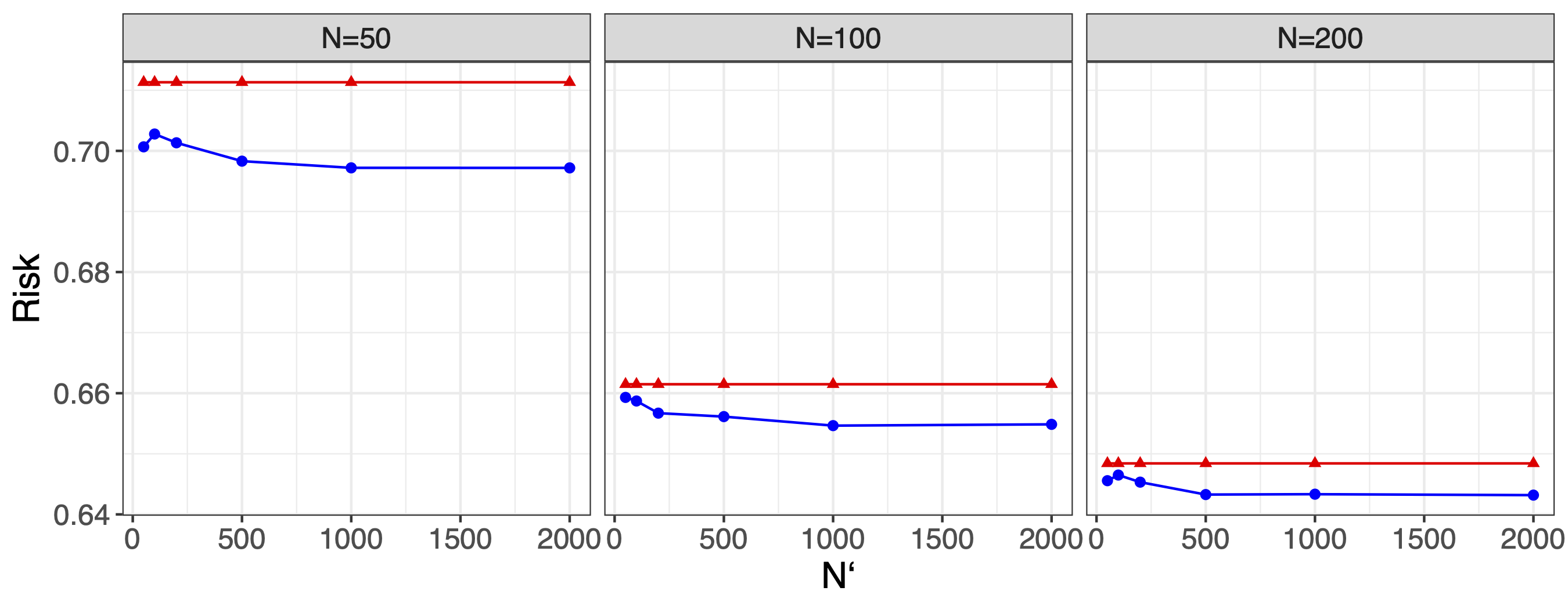
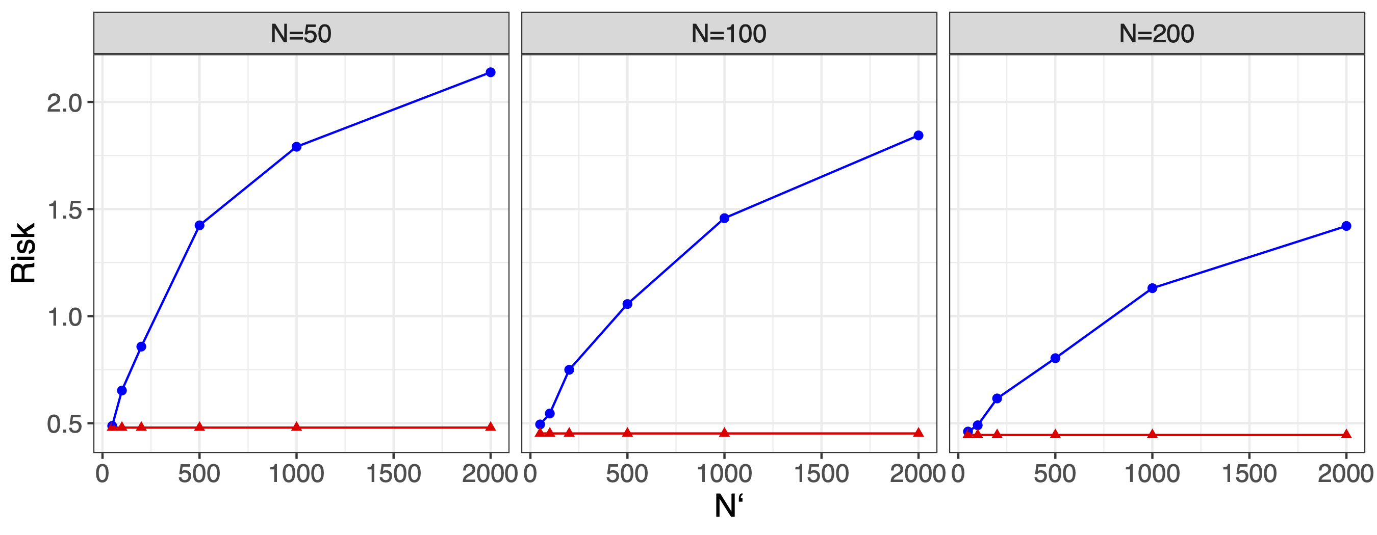
  • Fix N{50,100,200}𝑁50100200N\in\{50,100,200\} and vary N{50,100N^{\prime}\in\{50,100, 200,500,1000,2000}200,500,1000,2000\}.

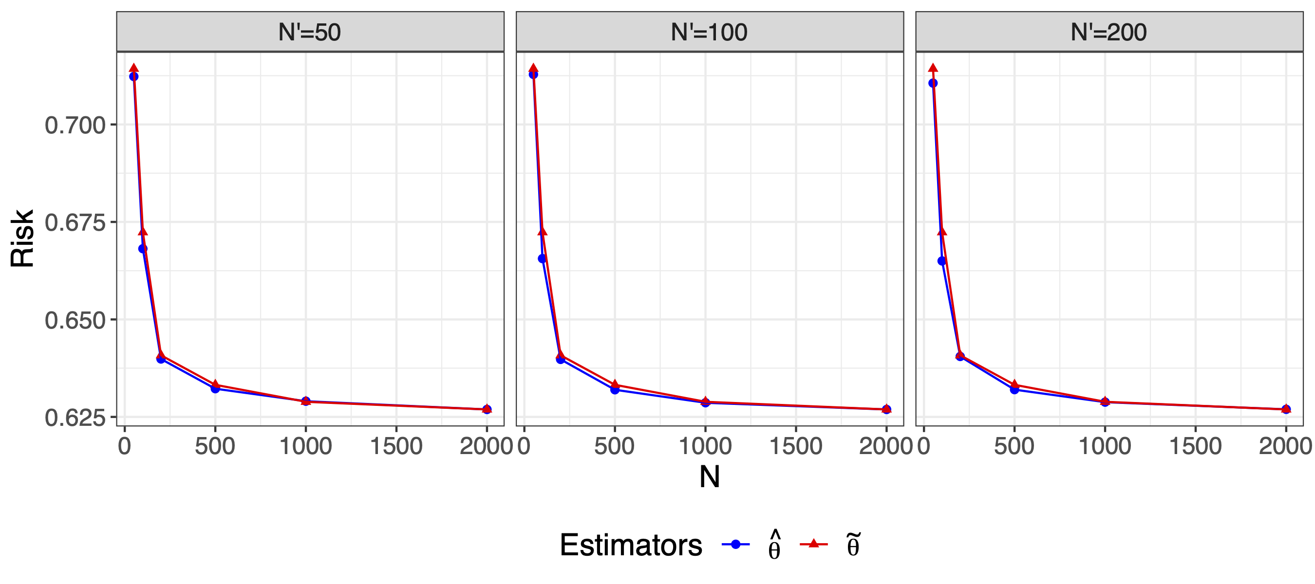
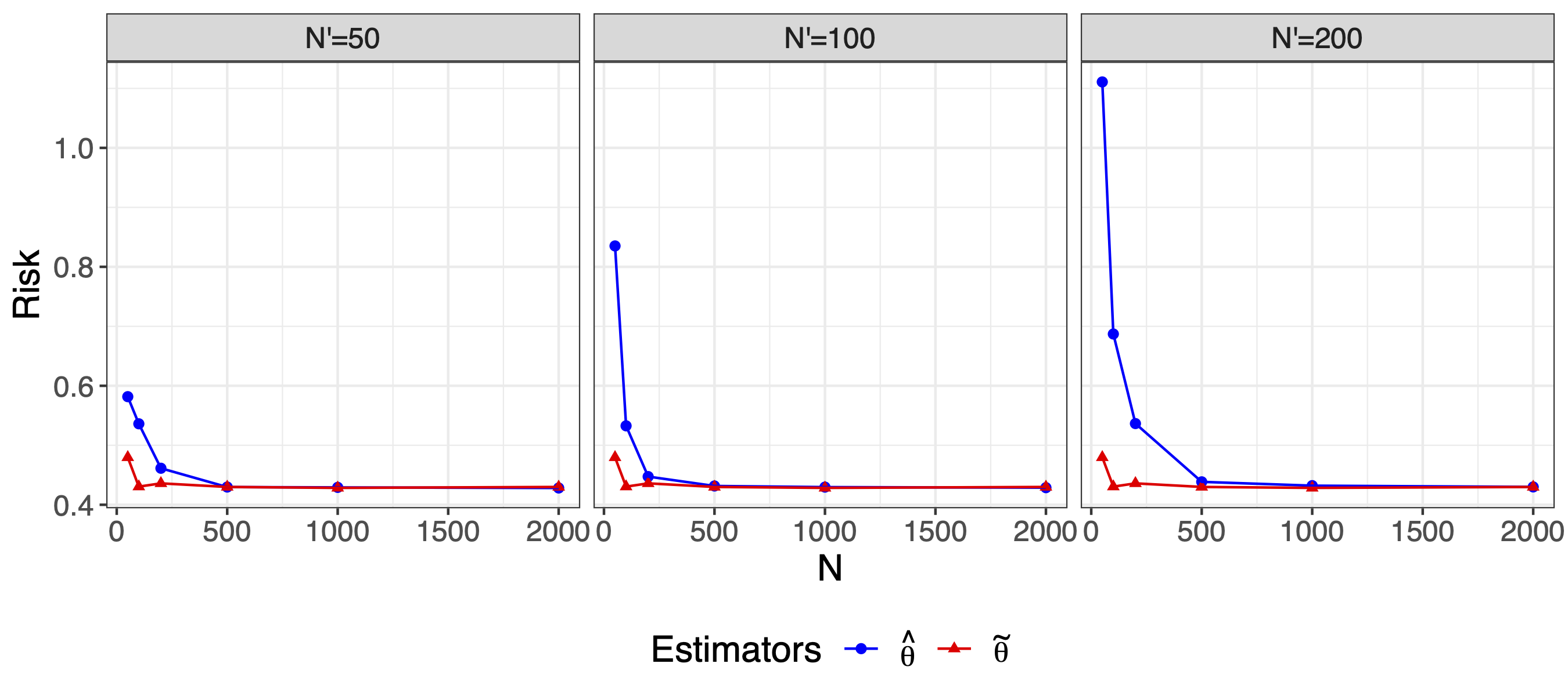
  • Fix N{50,100,200}superscript𝑁50100200N^{\prime}\in\{50,100,200\} and vary N{50,100N\in\{50,100, 200,500,1000,2000}200,500,1000,2000\}

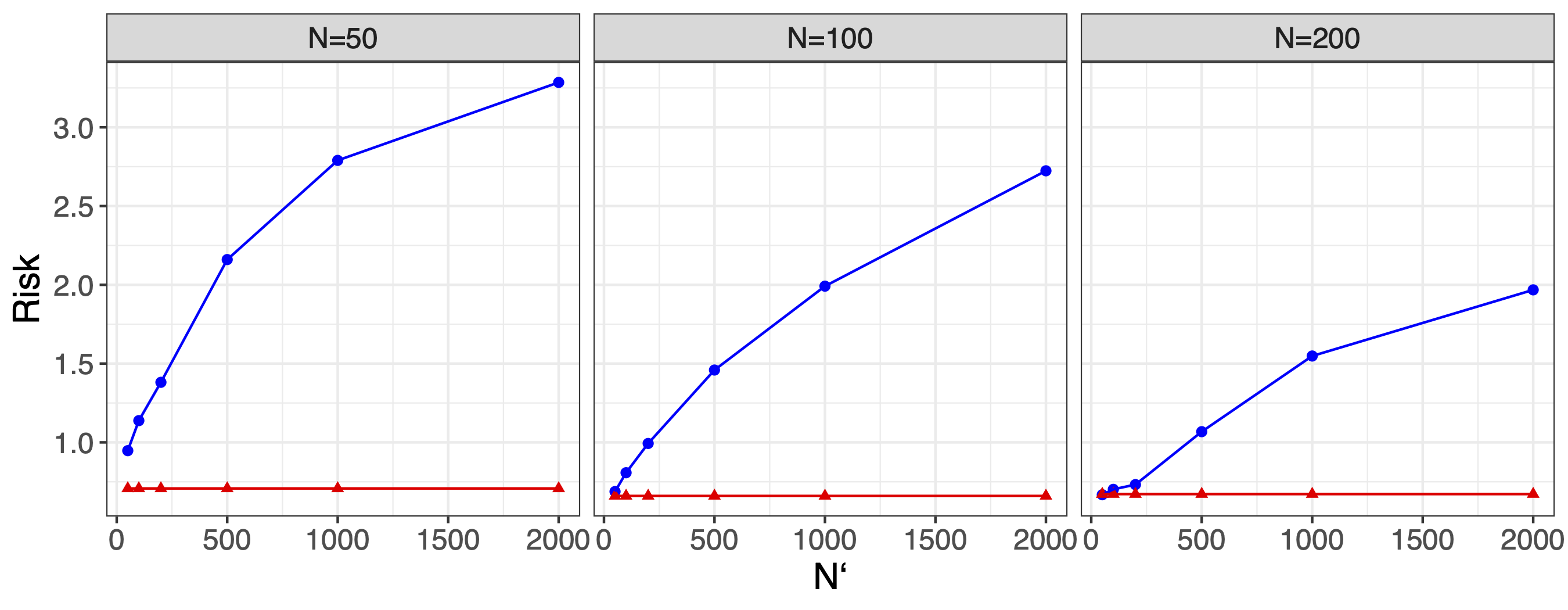
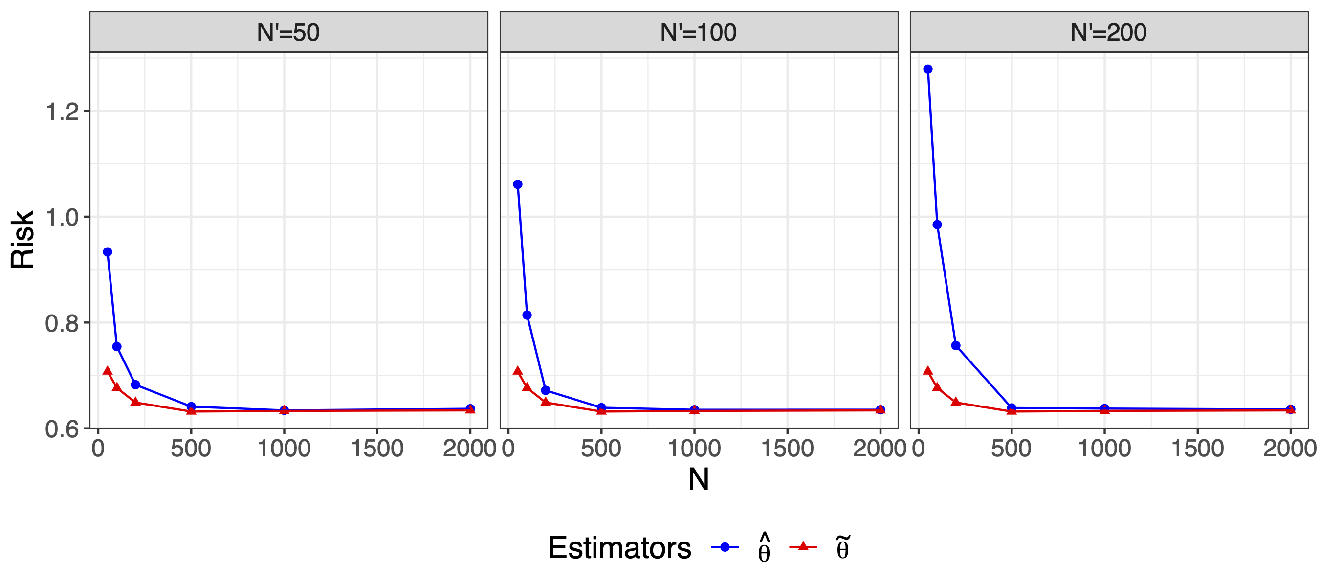
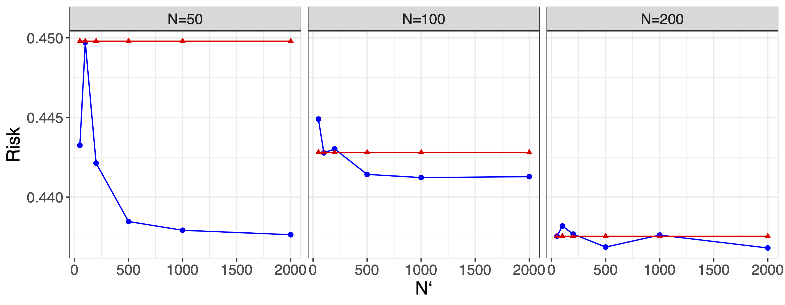
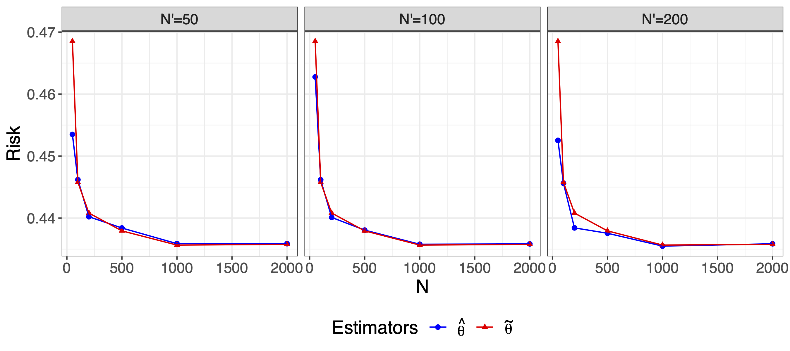
The results are shown in Figure 1 and Figure 2 for disjoint index sets. Overall, as we increase k𝑘k while fixing other parameters, the risk of both 𝜽^^𝜽\hat{\bm{\theta}} and 𝜽~~𝜽\tilde{\bm{\theta}} increases, which is as expected since we aim to capture the variability at a finer level with the same sample size. The first row of the plot for both scenarios represents the case when we fix N𝑁N and vary Nsuperscript𝑁N^{\prime}. Note that the sufficient condition for the dominance of 𝜽^^𝜽\hat{\bm{\theta}} is not satisfied in i, and we notice some cases where 𝜽~~𝜽\tilde{\bm{\theta}} has a lower risk when Nsuperscript𝑁N^{\prime} is relatively small. In contrast, 𝜽^^𝜽\hat{\bm{\theta}} outperforms 𝜽~~𝜽\tilde{\bm{\theta}} overall in ii even when Nsuperscript𝑁N^{\prime} is small. The second row represents the case when we fix Nsuperscript𝑁N^{\prime} and vary N𝑁N. The risk decreases drastically as N𝑁N increases due to the fact that we incorporate more and more observations that are fully classified.

Figure 3 and Figure 4 display the Bayes risk of 𝜽^1subscript^𝜽1\hat{\bm{\theta}}_{1} and 𝜽^2subscript^𝜽2\hat{\bm{\theta}}_{2} estimated using Gibbs sampling. Overall, we observe that 𝜽^^𝜽\hat{\bm{\theta}} has a higher risk than 𝜽~~𝜽\tilde{\bm{\theta}}, particularly when Nsuperscript𝑁N^{\prime} is large. When Nsuperscript𝑁N^{\prime} is fixed, increasing N𝑁N leads to a decrease in the risk of 𝜽^^𝜽\hat{\bm{\theta}}, as incorporating more fully classified data reduces the uncertainties introduced by adding Nsuperscript𝑁N^{\prime}.

We test our data disaggregation approach on two empirical examples, where we utilize data from the Sample Registration System (SRS) and Demographic and Health Surveys (DHS) as the sources of information, respectively.
Refer to caption
Refer to caption
Figure 1: Comparison of risk between 𝜽^1subscriptbold-^𝜽1\bm{\hat{\theta}}_{1} and 𝜽~1subscriptbold-~𝜽1\bm{\tilde{\theta}}_{1} estimators in simulation i.
Refer to caption
Refer to caption
Figure 2: Comparison of risk between 𝜽^2subscriptbold-^𝜽2\bm{\hat{\theta}}_{2} and 𝜽~2subscriptbold-~𝜽2\bm{\tilde{\theta}}_{2} estimators in simulation ii.
Refer to caption
Refer to caption
Figure 3: Comparison of risk between 𝜽^1subscriptbold-^𝜽1\bm{\hat{\theta}}_{1} and 𝜽~1subscriptbold-~𝜽1\bm{\tilde{\theta}}_{1} estimators in simulation iii.
Refer to caption
Refer to caption
Figure 4: Comparison of risk between 𝜽^2subscriptbold-^𝜽2\bm{\hat{\theta}}_{2} and 𝜽~2subscriptbold-~𝜽2\bm{\tilde{\theta}}_{2} estimators in simulation iv.

3.2 MCHSS Data of China

In this section, we provide the first empirical example using MCHSS data (Schumacher et al., 2020) obtained through China’s sample registration system dedicated to maternal and child health. Over a span of 20 years, from 1996 to 2015, all deaths of children under five years of age residing within the surveillance areas were recorded and grouped into six distinct age categories: 0-6 days, 7-27 days, 1-5 months, 6-11 months, 12-23 months, and 24-59 months, with eight non-overlapping, exhaustive categories of CODs.

To demonstrate the effectiveness of our disaggregation method under a nested age structure, we create a synthetic dataset based on the MCHSS data collected during the period of 199619961996 to 200520052005. In the synthetic dataset, the ages are partially classified into three groups: (i) 0-27 days, (ii) 1-11 months, and (iii) 12-59 months. Our goal is to use the fully classified MCHSS data collected from 200620062006 to 201520152015 to perform age group disaggregation.

True 1996-2005 MCHSS Data
1 2 3 4 5 6
1 3550 638 138 9 2 0
2 4398 183 24 0 0 0
3 1783 568 732 373 264 270
4 95 78 459 224 268 473
5 732 231 463 176 584 1333
6 39 92 501 361 270 196
7 1227 991 1671 570 428 328
8 1051 722 491 269 230 261
Predicted 1996-2005 MCHSS Data
1 2 3 4 5 6
1 3474 714 145 2 1 1
2 4258 323 23 1 0 0
3 1659 692 740 365 291 243
4 101 72 454 229 274 467
5 572 391 471 168 667 1250
6 26 105 536 326 321 145
7 1094 1124 1635 606 435 321
8 1059 714 515 245 243 248
Table 2: Comparison of true and disaggregated MCHSS data using Bayesian age reconciliation for the years 1996-2005.

We evaluate the effectiveness of our proposed Bayesian age reconciliation method by comparing its predicted results to the actual MCHSS data from 1996 to 2005, as shown in Table 2. We also compare the accuracy of our method to the data integration by random assignment approach. Our findings demonstrate that our method performs well, achieving a prediction accuracy of 93.0%percent93.093.0\% while only 52.6%percent52.652.6\% of the observations are classified correctly using the random assignment. These results highlights our method’s ability to preserve the joint COD-age distribution information with high accuracy.

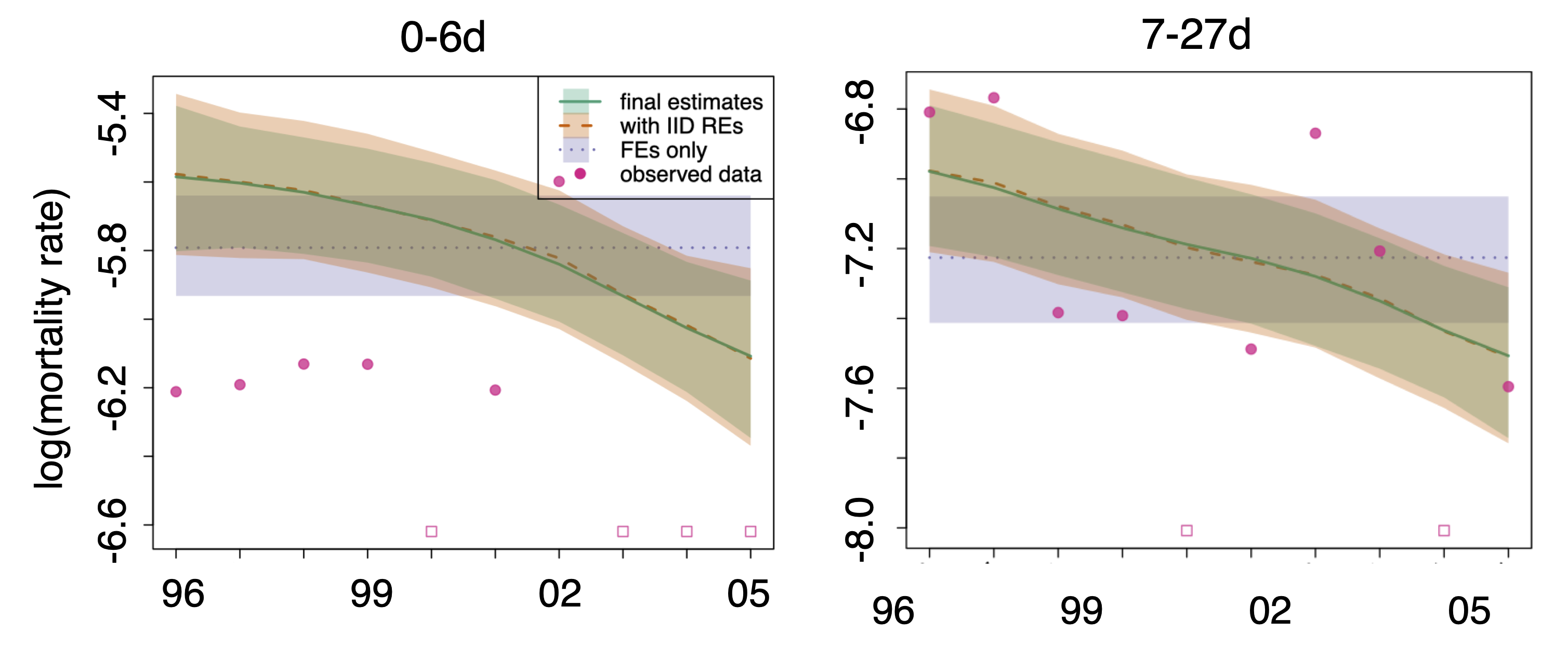
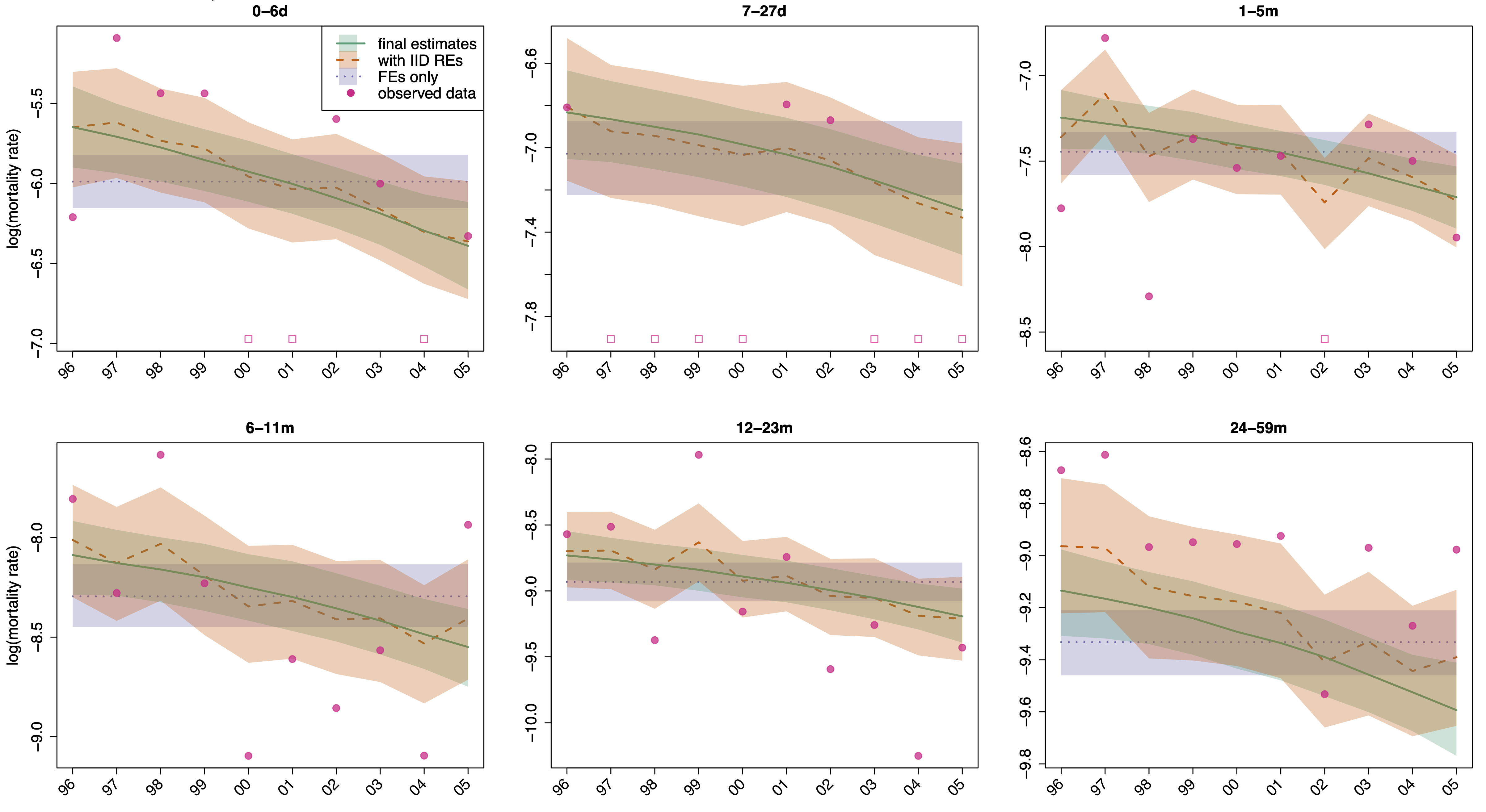
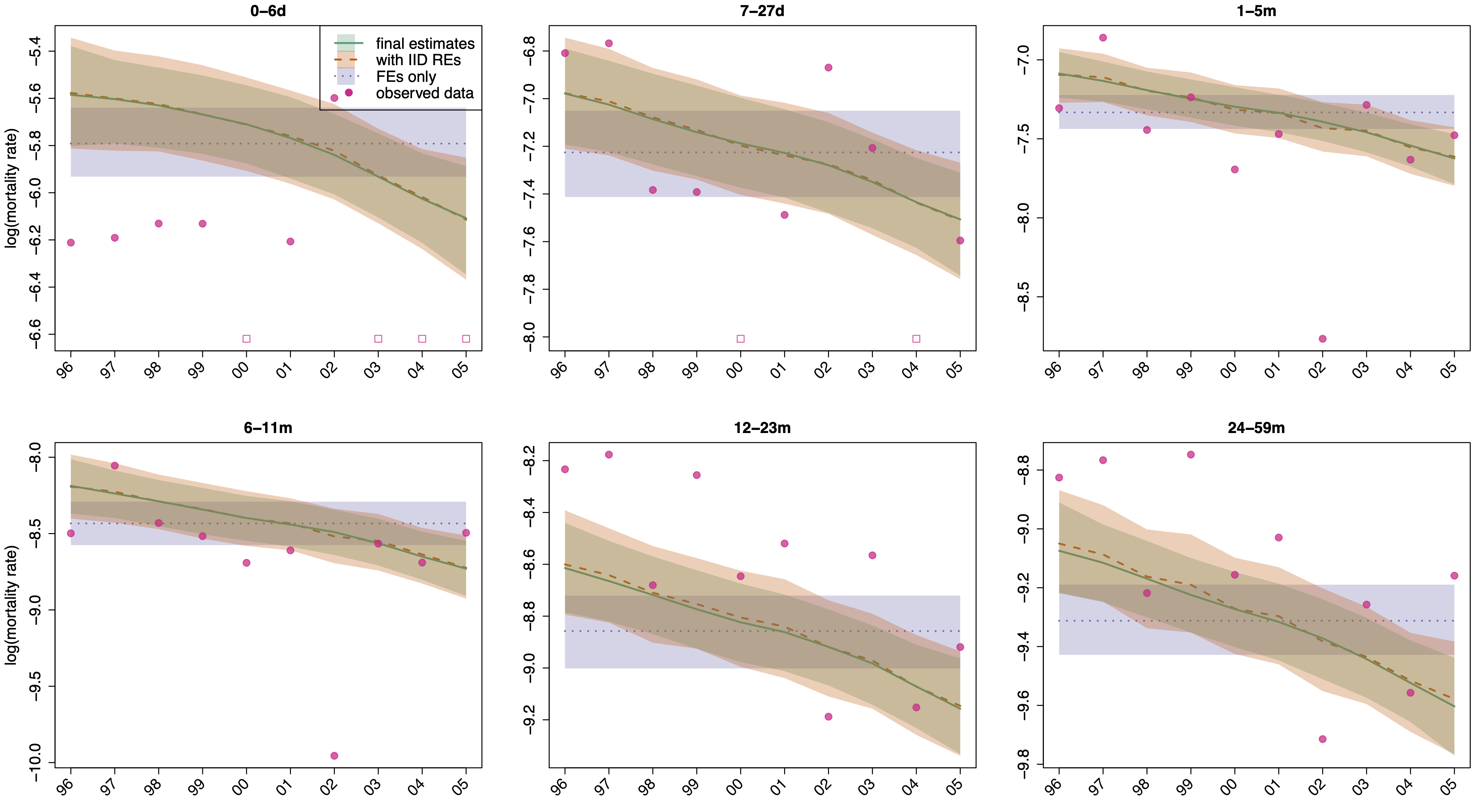
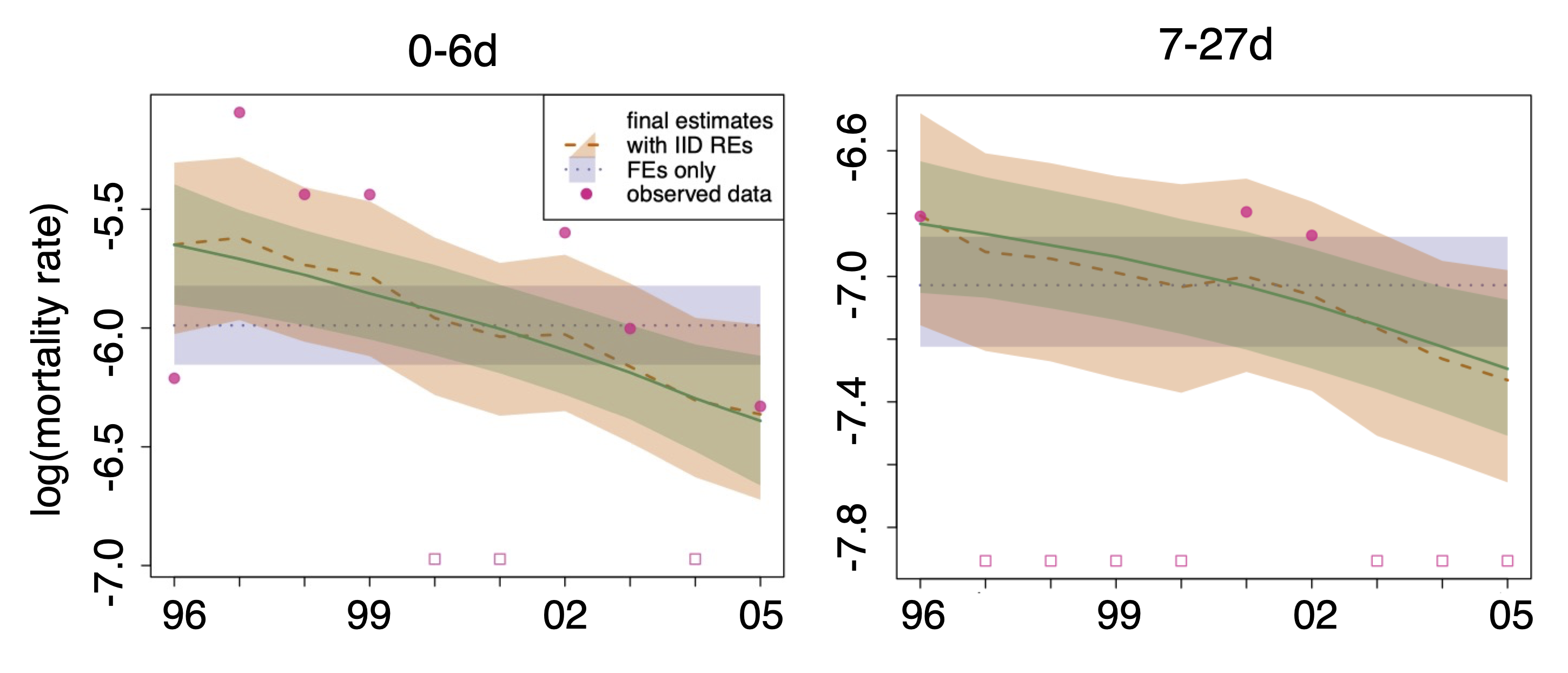
To examine the impact of utilizing the disaggregated data on the estimation of age- and cause-specific child mortality, we fit separate Bayesian models to the true and predicted 1996-2005 MCHSS data, as proposed by Schumacher et al. (2020). Figures 5 present the posterior medians and 80%percent8080\% intervals for the estimated log mortality rates in each age group over the period of 1996-2005 based on the true and predicted data in selected causes and ages. Additionally, we provide posterior median and 80%percent8080\% intervals for the estimated log mortality rates in models with fixed effects only and models with added random effect error terms, as previously discussed in Schumacher et al. (2020).
True 1996-2005 MCHSS Data
Refer to caption
Predicted 1996-2005 MCHSS Data
Refer to caption
Figure 5: Estimation of log mortality rates for non-communicable diseases in the east urban region using MCHSS data. The plot shows empirical data, estimated posterior medians, and posterior 80% intervals. Combinations with zero deaths are indicated by an open square.
True 1996-2005 MCHSS Data
Refer to caption
Predicted 1996-2005 MCHSS Data
Refer to caption
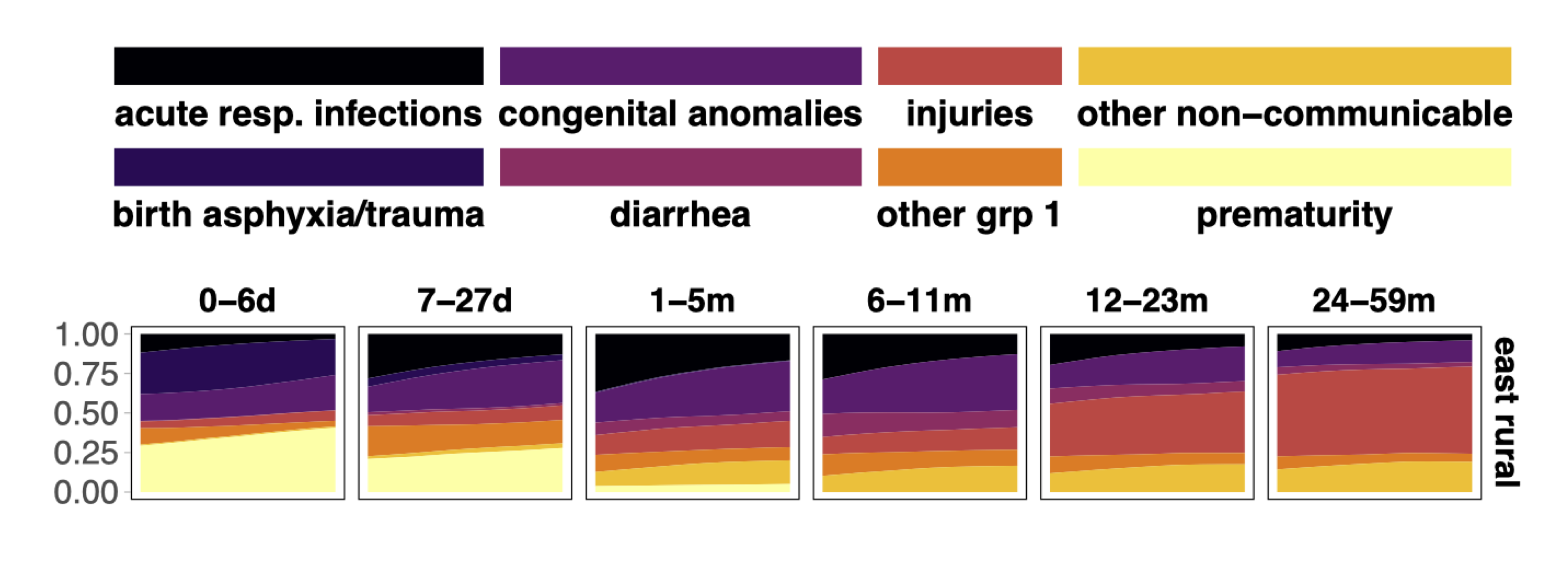
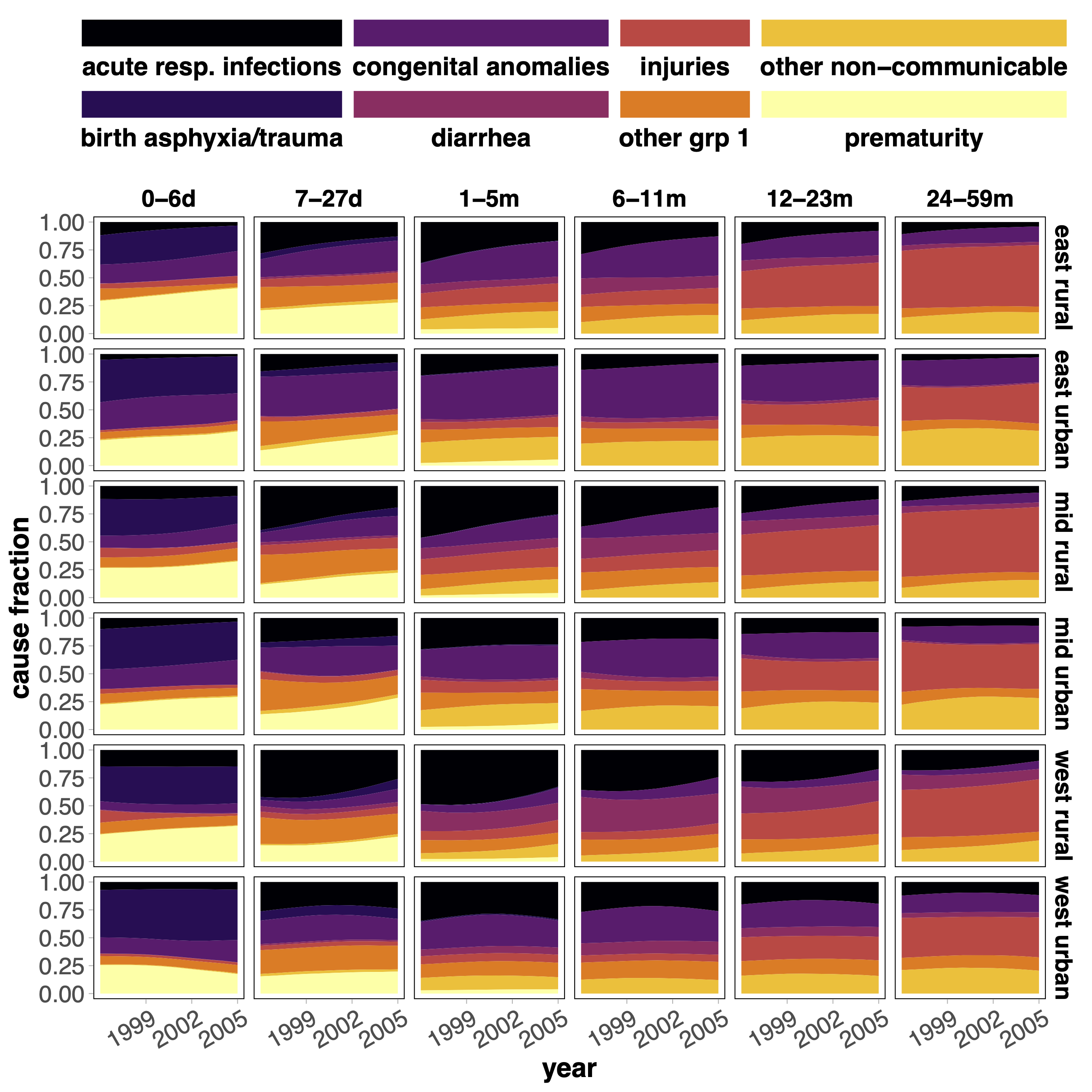
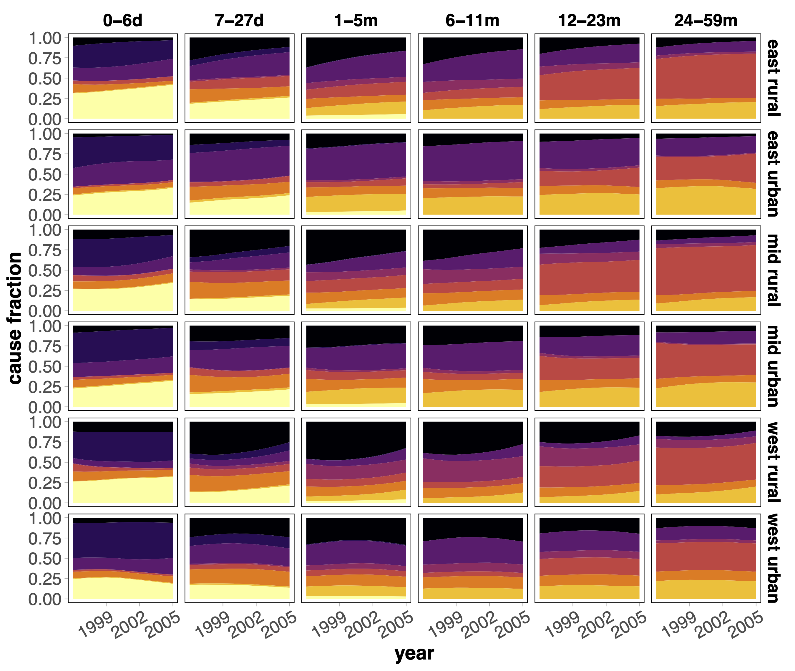
Figure 6: Comparisons of estimated CSMFs between models based the true MCHSS data and the estimated MCHSS data for selected regions, showing agreement in temporal trends and estimated CSMFs.

Figure 5 shows the results of the analysis of non-communicable diseases in the 0-6 days and 7-27 days age groups. Both the true and predicted data fit the models well, but some discrepancies are observed. Specifically, the estimated log mortality rates in the 0-6 days age group are consistently higher when using the predicted data compared to the true data. This discrepancy may be due to some deaths being incorrectly classified in the 7-27 days age group during the disaggregation process. However, the model fitted to the predicted data effectively captures the overall age-specific time trend and benefits from borrowing strength from other age strata.

Furthermore, in Figure 6, the estimated cause-specific mortality fractions (CSMFs) in the selected region are compared between the model fit of the real MCHSS data and the predicted data. This comparison demonstrates that the temporal trends and the estimated CSMFs from the model fit of the predicted data are in agreement with those of the true data.

3.3 BDHS Data

The BDHS data was collected through VA questionnaires in 2011, as well as in 2017-2018. Physical reviews were performed to determine the COD for each individual, with 11 common CODs being recorded. The ages at death for each individual were also documented. To demonstrate the effectiveness of our proposed method under a non-nested age structure, we aggregated the 2011 data into non-standard age categories: (i) 0-3 months, (ii) 4-11 months, and (iii) 12-59 months. For the 2017-2018 data, we created standardized age-disaggregated data with six age groups, as listed in Table 1.

Table 3 presents the comparison between the actual and predicted 2011 BDHS data, which shows overall satisfactory results, albeit with a few instances of misclassification in the non-nested age categories. Our proposed method achieved a slightly improved prediction accuracy of 70.4%percent70.470.4\%, compared to 54.9%percent54.954.9\% with random assignment.

True 2011 BDHS data
1 2 3 4 5 6
1 4 4 0 0 0 0
2 1 3 0 0 0 0
3 0 0 0 1 13 12
4 55 2 0 0 0 0
5 9 0 0 0 0 0
6 0 0 4 2 4 0
7 22 21 39 14 6 7
8 5 5 0 0 0 0
9 26 5 0 0 0 0
10 44 14 0 0 0 0
11 0 0 1 1 0 0
Predicted 2011 BDHS data
1 2 3 4 5 6
1 4 3 1 0 0 0
2 2 1 1 0 0 0
3 0 0 0 1 13 12
4 55 2 0 0 0 0
5 8 1 0 0 0 0
6 0 0 4 2 2 2
7 23 13 57 3 2 11
8 7 3 0 0 0 0
9 26 4 1 0 0 0
10 31 23 4 0 0 0
11 0 1 1 0 0 0
Table 3: Evaluating proposed method for non-standard age categories using 2011 BDHS data: comparison of actual and predicted results demonstrates promising performance with some misclassification observed.

4 Discussion

In this work, we extend the existing literature on simultaneous estimation of multinomial probabilities to a broader and more versatile setting. We provide theoretical support and numerical studies, demonstrating how the integration of partially classified data can lead to improved Bayesian estimators of multinomial probabilities. Our proposed age reconciliation method is based on this approach and has been tested through simulation studies using observed, disaggregated data. The results show that our method is promising and offers a novel perspective on mitigating age inconsistencies in ACSU5M studies.

Our proposed age reconciliation method is a promising first step in tackling the problem of age inconsistencies in ACSU5M studies. However, there are several future directions for research that could further address this issue. First, the CODs are commonly assigned and analyzed by statistical algorithms. For example, several Bayesian methods have been developed to infer CODs based on verbal autopsies (e.g, McCormick et al., 2016; Kunihama et al., 2020; Li et al., 2021; Wu et al., 2021) and estimate the population-level cause specific mortality fractions (e.g, Serina et al., 2015; Byass et al., 2019; Moran et al., 2021). However, it has been shown that considerable uncertainties exist in the classification in these models. One possible extension of our proposed method is to account for misclassifications in both CODs and age groups through the use of joint misclassification matrices in the model parameter estimations. This can be done by extending Bayesian hierarchical models such as the one proposed by Mulick et al. (2021). Our proposed method can extend the approach by accounting for misclassifcations from both CODs and age groups through of use of joint misclassification matrices in the model parameter estimations. Second, although our proposed method offers improved estimators under certain conditions, it fails to provide information theoretic metrics that quantify the effects of data disaggregation. One possible extension of the current approach is to use Dampster-Shafer inference (Dempster and Shafer, 1976) procedures as an alternative approach for multinomial inference (Lawrence et al., 2009). This approach can incorporate epistemic uncertainty and have the potential to quantify the effects of adding partial-classified multinomial data as adversarial attacks. Overall, we believe that these future research directions can further improve the accuracy and reliability of age reconciliations in ACSU5M studies.

References

  • Diaz et al. [2021] Theresa Diaz, Kathleen L Strong, Bochen Cao, Regina Guthold, Allisyn C Moran, Ann-Beth Moller, Jennifer Requejo, Ritu Sadana, Jotheeswaran Amuthavalli Thiyagarajan, Emmanuel Adebayo, et al. A call for standardised age-disaggregated health data. The Lancet Healthy Longevity, 2(7):e436–e443, 2021.
  • Fienberg and Holland [1973] Stephen E Fienberg and Paul W Holland. Simultaneous estimation of multinomial cell probabilities. Journal of the American Statistical Association, 68(343):683–691, 1973.
  • Leonard [1977] Tom Leonard. A bayesian approach to some multinomial estimation and pretesting problems. Journal of the American Statistical Association, 72(360a):869–874, 1977.
  • Alam and Mitra [1986] Khursheed Alam and Amitava Mitra. An empirical bayes estimate of multinomial probabilities. Communications in Statistics-Theory and Methods, 15(10):3103–3127, 1986.
  • Albert [1987] James H Albert. Empirical bayes estimation in contingency tables. Communications in Statistics-Theory and Methods, 16(8):2459–2485, 1987.
  • Chen and Fienberg [1976] Tar Chen and Stephen E Fienberg. The analysis of contingency tables with incompletely classified data. Biometrics, pages 133–144, 1976.
  • Albert [1985] James H Albert. Bayesian estimation methods for incomplete two-way contingency tables using prior belief of association. in “bayesian statistics”(jm bernardo,… and afm smith, eds.). Amsterdam, North Holland, 2:589–602, 1985.
  • Gibbons and Greenberg [1994] Patrick C Gibbons and Edward Greenberg. Bayesian reconstruction of contingency tables with partially categorized data. Communications in Statistics-Theory and Methods, 23(12):3349–3359, 1994.
  • Ahn et al. [2010] Kwang Woo Ahn, Kung-Sik Chan, Ying Bai, and Michael Kosoy. Bayesian inference with incomplete multinomial data: A problem in pathogen diversity. Journal of the American Statistical Association, 105(490):600–611, 2010.
  • Nayak and Naik [1989] Tapan K Nayak and Dayanand N Naik. Estimating multinomial cell probabilities under quadratic loss. Journal of the Royal Statistical Society: Series D (The Statistician), 38(1):3–10, 1989.
  • Ishwaran and James [2001] Hemant Ishwaran and Lancelot F James. Gibbs sampling methods for stick-breaking priors. Journal of the American statistical Association, 96(453):161–173, 2001.
  • Doshi et al. [2009] Finale Doshi, Kurt Miller, Jurgen Van Gael, and Yee Whye Teh. Variational inference for the indian buffet process. In Artificial Intelligence and Statistics, pages 137–144. PMLR, 2009.
  • Teh et al. [2010] Yee Whye Teh et al. Dirichlet process. Encyclopedia of machine learning, 1063:280–287, 2010.
  • Gelfand [2000] Alan E Gelfand. Gibbs sampling. Journal of the American statistical Association, 95(452):1300–1304, 2000.
  • Schumacher et al. [2020] Austin E Schumacher, Tyler H McCormick, Jon Wakefield, Yue Chu, Jamie Perin, Francisco Villavicencio, Noah Simon, and Li Liu. A flexible bayesian framework to estimate age-and cause-specific child mortality over time from sample registration data. arXiv preprint arXiv:2003.00401, 2020.
  • McCormick et al. [2016] Tyler H McCormick, Zehang Richard Li, Clara Calvert, Amelia C Crampin, Kathleen Kahn, and Samuel J Clark. Probabilistic cause-of-death assignment using verbal autopsies. Journal of the American Statistical Association, 111(515):1036–1049, 2016.
  • Kunihama et al. [2020] Tsuyoshi Kunihama, Zehang Richard Li, Samuel J Clark, and Tyler H McCormick. Bayesian factor models for probabilistic cause of death assessment with verbal autopsies. The annals of applied statistics, 14(1):241, 2020.
  • Li et al. [2021] Zehang Richard Li, Zhenke Wu, Irena Chen, and Samuel J Clark. Bayesian nested latent class models for cause-of-death assignment using verbal autopsies across multiple domains. arXiv preprint arXiv:2112.12186, 2021.
  • Wu et al. [2021] Zhenke Wu, Zehang Richard Li, Irena Chen, and Mengbing Li. Tree-informed bayesian multi-source domain adaptation: cross-population probabilistic cause-of-death assignment using verbal autopsy. arXiv preprint arXiv:2112.10978, 2021.
  • Serina et al. [2015] Peter Serina, Ian Riley, Andrea Stewart, Spencer L James, Abraham D Flaxman, Rafael Lozano, Bernardo Hernandez, Meghan D Mooney, Richard Luning, Robert Black, et al. Improving performance of the Tariff method for assigning causes of death to verbal autopsies. BMC Medicine, 13(1):1, 2015.
  • Byass et al. [2019] Peter Byass, Laith Hussain-Alkhateeb, Lucia D’Ambruoso, Samuel Clark, Justine Davies, Edward Fottrell, Jon Bird, Chodziwadziwa Kabudula, Stephen Tollman, Kathleen Kahn, Schiőler Linus, and Max Petzold. An integrated approach to processing WHO-2016 verbal autopsy data: the InterVA-5 model. BMC Medicine, 17(1):1–12, 2019.
  • Moran et al. [2021] Kelly R. Moran, Elizabeth L. Turner, David Dunson, and Amy H. Herring. Bayesian hierarchical factor regression models to infer cause of death from verbal autopsy data. Journal of the Royal Statistical Society: Series C (Applied Statistics), 70(3):532–557, June 2021. ISSN 0035-9254. doi:10.1111/rssc.12468.
  • Mulick et al. [2021] Amy R Mulick, Shefali Oza, David Prieto-Merino, Francisco Villavicencio, Simon Cousens, and Jamie Perin. A bayesian hierarchical model with integrated covariate selection and misclassification matrices to estimate neonatal and child causes of death. medRxiv, pages 2021–02, 2021.
  • Dempster and Shafer [1976] A.P. Dempster and G. Shafer. A Mathematical Theory of Evidence. Limited paperback editions. Princeton University Press, 1976. ISBN 9780691100425. URL https://books.google.com/books?id=wug9DwAAQBAJ.
  • Lawrence et al. [2009] Earl Lawrence, Chunhai Liu, Scott Vander Wiel, and J Zhang. A new method of multinomial inference using dempster-shafer theory. Unpublished Manuscript, 2009.

Supplementary Material to “Bayesian Age Category Reconciliation for Age- and Cause-specific Under-five Mortality Estimates”

S.1 Proof of Lemma 1

Let 𝝆Aj=(θiτj,iAj)Tsubscript𝝆subscript𝐴𝑗superscriptsubscript𝜃𝑖subscript𝜏𝑗𝑖subscript𝐴𝑗𝑇\bm{\rho}_{A_{j}}=(\frac{\theta_{i}}{\tau_{j}},i\in A_{j})^{T}, j=0,,m𝑗0𝑚j=0,\dots,m be the conditional probabilities of each individual cell within each group Ajsubscript𝐴𝑗A_{j} and 𝜼=(𝝉,𝝆Aj,j=0,,m)\bm{\eta}=(\bm{\tau},\bm{\rho}_{A_{j}},j=0,\dots,m) The probability mass function of (𝑿,𝒀)=(X1,X2,,Xk,YA1,,YAm)𝑿𝒀subscript𝑋1subscript𝑋2subscript𝑋𝑘subscript𝑌subscript𝐴1subscript𝑌𝐴𝑚(\bm{X},\bm{Y})=(X_{1},X_{2},\dots,X_{k},Y_{A_{1}},\dots,Y_{Am}) is

f(𝑿,𝒀|𝜼)𝑓𝑿conditional𝒀𝜼\displaystyle f(\bm{X},\bm{Y}|\bm{\eta}) =(N!i=1kXi!i=1kθiXi)N!j=0mYAj!j=0mτjYAjabsent𝑁superscriptsubscriptproduct𝑖1𝑘subscript𝑋𝑖superscriptsubscriptproduct𝑖1𝑘superscriptsubscript𝜃𝑖subscript𝑋𝑖superscript𝑁superscriptsubscriptproduct𝑗0𝑚subscript𝑌subscript𝐴𝑗superscriptsubscriptproduct𝑗0𝑚superscriptsubscript𝜏𝑗subscript𝑌subscript𝐴𝑗\displaystyle=\left(\frac{N!}{\prod_{i=1}^{k}X_{i}!}\prod_{i=1}^{k}\theta_{i}^{X_{i}}\right)\frac{N^{\prime}!}{\prod_{j=0}^{m}Y_{A_{j}}!}\prod_{j=0}^{m}\tau_{j}^{Y_{A_{j}}}
=N!i=1kXi!N!j=0mYAj!{rA0(τ0ρA0(r))Xr×rA1(τ1ρA1(r))Xr××rAm(τmρAm(r))Xr}j=0mτjYAjabsent𝑁superscriptsubscriptproduct𝑖1𝑘subscript𝑋𝑖superscript𝑁superscriptsubscriptproduct𝑗0𝑚subscript𝑌subscript𝐴𝑗subscriptproduct𝑟subscript𝐴0superscriptsubscript𝜏0superscriptsubscript𝜌subscript𝐴0𝑟subscript𝑋𝑟subscriptproduct𝑟subscript𝐴1superscriptsubscript𝜏1superscriptsubscript𝜌subscript𝐴1𝑟subscript𝑋𝑟subscriptproduct𝑟subscript𝐴𝑚superscriptsubscript𝜏𝑚superscriptsubscript𝜌subscript𝐴𝑚𝑟subscript𝑋𝑟superscriptsubscriptproduct𝑗0𝑚superscriptsubscript𝜏𝑗subscript𝑌subscript𝐴𝑗\displaystyle=\frac{N!}{\prod_{i=1}^{k}X_{i}!}\frac{N^{\prime}!}{\prod_{j=0}^{m}Y_{A_{j}}!}\left\{\prod_{r\in A_{0}}(\tau_{0}\rho_{A_{0}}^{(r)})^{X_{r}}\times\prod_{r\in A_{1}}(\tau_{1}\rho_{A_{1}}^{(r)})^{X_{r}}\times\dots\times\prod_{r\in A_{m}}(\tau_{m}\rho_{A_{m}}^{(r)})^{X_{r}}\right\}\prod_{j=0}^{m}\tau_{j}^{Y_{A_{j}}}
=N!i=1kXi!N!j=0mYAj!(j=0mrAj(τjρAj(r))Xr)j=0mτjYAjabsent𝑁superscriptsubscriptproduct𝑖1𝑘subscript𝑋𝑖superscript𝑁superscriptsubscriptproduct𝑗0𝑚subscript𝑌subscript𝐴𝑗superscriptsubscriptproduct𝑗0𝑚subscriptproduct𝑟subscript𝐴𝑗superscriptsubscript𝜏𝑗superscriptsubscript𝜌subscript𝐴𝑗𝑟subscript𝑋𝑟superscriptsubscriptproduct𝑗0𝑚superscriptsubscript𝜏𝑗subscript𝑌subscript𝐴𝑗\displaystyle=\frac{N!}{\prod_{i=1}^{k}X_{i}!}\frac{N^{\prime}!}{\prod_{j=0}^{m}Y_{A_{j}}!}\left(\prod_{j=0}^{m}\prod_{r\in A_{j}}(\tau_{j}\rho_{A_{j}}^{(r)})^{X_{r}}\right)\prod_{j=0}^{m}\tau_{j}^{Y_{A_{j}}}
=N!i=1kXi!N!j=0mYAj!(j=0mτjrAjXr+YAj)j=0mrAj(ρAj(r))Xrabsent𝑁superscriptsubscriptproduct𝑖1𝑘subscript𝑋𝑖superscript𝑁superscriptsubscriptproduct𝑗0𝑚subscript𝑌subscript𝐴𝑗superscriptsubscriptproduct𝑗0𝑚superscriptsubscript𝜏𝑗subscript𝑟subscript𝐴𝑗subscript𝑋𝑟subscript𝑌subscript𝐴𝑗superscriptsubscriptproduct𝑗0𝑚subscriptproduct𝑟subscript𝐴𝑗superscriptsuperscriptsubscript𝜌subscript𝐴𝑗𝑟subscript𝑋𝑟\displaystyle=\frac{N!}{\prod_{i=1}^{k}X_{i}!}\frac{N^{\prime}!}{\prod_{j=0}^{m}Y_{A_{j}}!}\left(\prod_{j=0}^{m}\tau_{j}^{\sum_{r\in A_{j}}X_{r}+Y_{A_{j}}}\right)\prod_{j=0}^{m}\prod_{r\in A_{j}}(\rho_{A_{j}}^{(r)})^{X_{r}}
=N!i=1kXi!Nj=0mYAj!(j=0mτjXAj+YAj)j=0mrAj(ρAj(r))Xrabsent𝑁superscriptsubscriptproduct𝑖1𝑘subscript𝑋𝑖superscript𝑁superscriptsubscriptproduct𝑗0𝑚subscript𝑌subscript𝐴𝑗superscriptsubscriptproduct𝑗0𝑚superscriptsubscript𝜏𝑗subscript𝑋subscript𝐴𝑗subscript𝑌subscript𝐴𝑗superscriptsubscriptproduct𝑗0𝑚subscriptproduct𝑟subscript𝐴𝑗superscriptsuperscriptsubscript𝜌subscript𝐴𝑗𝑟subscript𝑋𝑟\displaystyle=\frac{N!}{\prod_{i=1}^{k}X_{i}!}\frac{N^{\prime}}{\prod_{j=0}^{m}Y_{A_{j}}!}\left(\prod_{j=0}^{m}\tau_{j}^{X_{A_{j}}+Y_{A_{j}}}\right)\prod_{j=0}^{m}\prod_{r\in A_{j}}(\rho_{A_{j}}^{(r)})^{X_{r}}

where XAj=rAjXrsubscript𝑋subscript𝐴𝑗subscript𝑟subscript𝐴𝑗subscript𝑋𝑟X_{A_{j}}=\sum_{r\in A_{j}}X_{r}.

log{j=0mrAj(ρAj(r))Xr}superscriptsubscriptproduct𝑗0𝑚subscriptproduct𝑟subscript𝐴𝑗superscriptsuperscriptsubscript𝜌subscript𝐴𝑗𝑟subscript𝑋𝑟\displaystyle\log\{\prod_{j=0}^{m}\prod_{r\in A_{j}}(\rho_{A_{j}}^{(r)})^{X_{r}}\} =log{rA0(ρA0(r))Xr×rA1(ρA1(r))Xr××rAm(ρAm(r))Xr}absentsubscriptproduct𝑟subscript𝐴0superscriptsuperscriptsubscript𝜌subscript𝐴0𝑟subscript𝑋𝑟subscriptproduct𝑟subscript𝐴1superscriptsuperscriptsubscript𝜌subscript𝐴1𝑟subscript𝑋𝑟subscriptproduct𝑟subscript𝐴𝑚superscriptsuperscriptsubscript𝜌subscript𝐴𝑚𝑟subscript𝑋𝑟\displaystyle=\log\{\prod_{r\in A_{0}}(\rho_{A_{0}}^{(r)})^{X_{r}}\times\prod_{r\in A_{1}}(\rho_{A_{1}}^{(r)})^{X_{r}}\times\dots\times\prod_{r\in A_{m}}(\rho_{A_{m}}^{(r)})^{X_{r}}\}
=j=0mlogrAj(ρAj(r))Xrabsentsuperscriptsubscript𝑗0𝑚subscriptproduct𝑟subscript𝐴𝑗superscriptsuperscriptsubscript𝜌subscript𝐴𝑗𝑟subscript𝑋𝑟\displaystyle=\sum_{j=0}^{m}\log\prod_{r\in A_{j}}(\rho_{A_{j}}^{(r)})^{X_{r}}
=j=0mrAjXrlog(ρAj(r))absentsuperscriptsubscript𝑗0𝑚subscript𝑟subscript𝐴𝑗subscript𝑋𝑟superscriptsubscript𝜌subscript𝐴𝑗𝑟\displaystyle=\sum_{j=0}^{m}\sum_{r\in A_{j}}X_{r}\log(\rho_{A_{j}}^{(r)})
=j=0mrAj\j0Xrlog(ρAj(r))+Xj0logρAjj0absentsuperscriptsubscript𝑗0𝑚subscript𝑟\subscript𝐴𝑗superscript𝑗0subscript𝑋𝑟superscriptsubscript𝜌subscript𝐴𝑗𝑟subscript𝑋superscript𝑗0subscriptsuperscriptsubscript𝜌subscript𝐴𝑗superscript𝑗0\displaystyle=\sum_{j=0}^{m}\sum_{r\in A_{j}\backslash j^{0}}X_{r}\log(\rho_{A_{j}}^{(r)})+X_{j^{0}}\log_{\rho_{A_{j}}^{j^{0}}}

where j0=Aj(0)superscript𝑗0superscriptsubscript𝐴𝑗0j^{0}=A_{j}^{(0)} is the first item of Ajsubscript𝐴𝑗A_{j}.

For rAj\j0𝑟\subscript𝐴𝑗subscript𝑗0r\in A_{j}\backslash j_{0}, j=0,,m𝑗0𝑚j=0,\dots,m:

ρAj(r)logf(𝑿,𝒀|𝜼)=XrρAj(r)Xj0ρAj(j0)superscriptsubscript𝜌subscript𝐴𝑗𝑟𝑓𝑿conditional𝒀𝜼subscript𝑋𝑟superscriptsubscript𝜌subscript𝐴𝑗𝑟subscript𝑋superscript𝑗0superscriptsubscript𝜌subscript𝐴𝑗superscript𝑗0\frac{\partial}{\rho_{A_{j}}^{(r)}}\log f(\bm{X},\bm{Y}|\bm{\eta})=\frac{X_{r}}{\rho_{A_{j}}^{(r)}}-\frac{X_{j^{0}}}{\rho_{A_{j}}^{(j^{0})}}

For r,rAj\j0𝑟superscript𝑟\subscript𝐴𝑗subscript𝑗0r,r^{\prime}\in A_{j}\backslash j_{0} and j=0,,m𝑗0𝑚j=0,\dots,m:

2(ρAj(r))(ρAj(r))logf(𝑿,𝒀|𝜼)={Xr(ρAj(r))2Xj0(ρAjj0)2 if r=rXr(ρAj(r))2 if rrsuperscript2superscriptsubscript𝜌subscript𝐴𝑗𝑟superscriptsubscript𝜌subscript𝐴𝑗superscript𝑟𝑓𝑿conditional𝒀𝜼casessubscript𝑋𝑟superscriptsuperscriptsubscript𝜌subscript𝐴𝑗𝑟2subscript𝑋superscript𝑗0superscriptsuperscriptsubscript𝜌subscript𝐴𝑗superscript𝑗02 if 𝑟superscript𝑟subscript𝑋𝑟superscriptsuperscriptsubscript𝜌subscript𝐴𝑗𝑟2 if 𝑟superscript𝑟\frac{\partial^{2}}{(\partial\rho_{A_{j}}^{(r)})(\partial\rho_{A_{j}}^{(r^{\prime})})}\log f(\bm{X},\bm{Y}|\bm{\eta})=\left\{\begin{array}[]{@{}l@{\quad}l@{}}-\frac{X_{r}}{(\rho_{A_{j}}^{(r)})^{2}}-\frac{X_{j^{0}}}{(\rho_{A_{j}}^{j^{0}})^{2}}&\mbox{ if }r=r^{\prime}\\ -\frac{X_{r}}{(\rho_{A_{j}}^{(r)})^{2}}&\mbox{ if }r\neq r^{\prime}\end{array}\right.

Let Ap={p1,,pnp}subscript𝐴𝑝subscript𝑝1subscript𝑝subscript𝑛𝑝A_{p}=\{p_{1},\dots,p_{n_{p}}\}, p=0,,m𝑝0𝑚p=0,\dots,m. For the p𝑝p-th group, the conditional vector of the cells within the group is ρAp=(θp1τp,,θpnpτp)subscript𝜌subscript𝐴𝑝subscript𝜃subscript𝑝1subscript𝜏𝑝subscript𝜃subscript𝑝subscript𝑛𝑝subscript𝜏𝑝\rho_{A_{p}}=(\frac{\theta_{p_{1}}}{\tau_{p}},\dots,\frac{\theta_{p_{n_{p}}}}{\tau_{p}}). Consider the Jeffrey’s prior, we have that

The Jefferys prior is

π(𝜼)d𝜼𝜋𝜼𝑑𝜼\displaystyle\pi(\bm{\eta})d\bm{\eta} |𝔼𝜽[diag(XA1+YA1τ12,,XAm+YAmτm2)+𝒊(m)(𝒊(m))TXA0+YA0τ02]|proportional-toabsentsubscript𝔼𝜽delimited-[]diagsubscript𝑋subscript𝐴1subscript𝑌subscript𝐴1superscriptsubscript𝜏12subscript𝑋subscript𝐴𝑚subscript𝑌subscript𝐴𝑚superscriptsubscript𝜏𝑚2superscript𝒊𝑚superscriptsuperscript𝒊𝑚𝑇subscript𝑋subscript𝐴0subscript𝑌subscript𝐴0superscriptsubscript𝜏02\displaystyle\propto\sqrt{\left|\mathbb{E}_{\bm{\theta}}\left[\mbox{diag}\left(\frac{X_{A_{1}}+Y_{A_{1}}}{\tau_{1}^{2}},\dots,\frac{X_{A_{m}}+Y_{A_{m}}}{\tau_{m}^{2}}\right)+\bm{i}^{(m)}(\bm{i}^{(m)})^{T}\frac{X_{A_{0}}+Y_{A_{0}}}{\tau_{0}^{2}}\right]\right|}
×j=0m|𝔼𝜽[diag(Xr(ρAj(r))2)rAj\j0+𝒊(nj1)(𝒊(nj1))TXj0(ρAj(j0))2]|\displaystyle\times\prod_{j=0}^{m}\sqrt{\left|\mathbb{E}_{\bm{\theta}}\left[\mbox{diag}\left(\frac{X_{r}}{(\rho_{A_{j}}^{(r)})^{2}}\right)_{r\in A_{j}\backslash j_{0}}+\bm{i}^{(n_{j}-1)}(\bm{i}^{(n_{j}-1)})^{T}\frac{X_{j^{0}}}{(\rho_{A_{j}}^{(j^{0})})^{2}}\right]\right|}
|diag(1τ1,,1τm)+𝒊(m)(𝒊(m))T1τ0|×(j=1m(τj)nj)proportional-toabsentdiag1subscript𝜏11subscript𝜏𝑚superscript𝒊𝑚superscriptsuperscript𝒊𝑚𝑇1subscript𝜏0superscriptsubscriptproduct𝑗1𝑚superscriptsubscript𝜏𝑗subscript𝑛𝑗\displaystyle\propto\sqrt{\left|\mbox{diag}\left(\frac{1}{\tau_{1}},\dots,\frac{1}{\tau_{m}}\right)+\bm{i}^{(m)}(\bm{i}^{(m)})^{T}\frac{1}{\tau_{0}}\right|}\times\left(\prod_{j=1}^{m}(\sqrt{\tau_{j}})^{n_{j}}\right)
×j=0m|diag(1ρAj(r))rAj\j0+𝒊(nj1)(𝒊(nj1))T1ρAj(j0)|\displaystyle\times\prod_{j=0}^{m}\sqrt{\left|\mbox{diag}\left(\frac{1}{\rho_{A_{j}}^{(r)}}\right)_{r\in A_{j}\backslash j^{0}}+\bm{i}^{(n_{j}-1)}(\bm{i}^{(n_{j}-1)})^{T}\frac{1}{\rho_{A_{j}}^{(j^{0})}}\right|}
=|diag(1τ1,,1τm)|[1+(𝒊(m))Tτ0{diag(1τ1,,1τm)}1𝒊(m)τ0]absentdiag1subscript𝜏11subscript𝜏𝑚delimited-[]1superscriptsuperscript𝒊𝑚𝑇subscript𝜏0superscriptdiag1subscript𝜏11subscript𝜏𝑚1superscript𝒊𝑚subscript𝜏0\displaystyle=\sqrt{\left|\mbox{diag}\left(\frac{1}{\tau_{1}},\dots,\frac{1}{\tau_{m}}\right)\right|\left[1+\frac{(\bm{i}^{(m)})^{T}}{\sqrt{\tau_{0}}}\left\{\mbox{diag}\left(\frac{1}{\tau_{1}},\dots,\frac{1}{\tau_{m}}\right)\right\}^{-1}\frac{\bm{i}^{(m)}}{\sqrt{\tau_{0}}}\right]}
×(j=1mτjnj/2)j=0m|diag(1ρAj(r))rAj\j0|[1+(𝒊(nj1))TρAj(j0){diag(1ρAj(r))rAj\j0}1𝒊(nj1)ρAj(j0)]absentsuperscriptsubscriptproduct𝑗1𝑚superscriptsubscript𝜏𝑗subscript𝑛𝑗2superscriptsubscriptproduct𝑗0𝑚diagsubscript1superscriptsubscript𝜌subscript𝐴𝑗𝑟𝑟\subscript𝐴𝑗superscript𝑗0delimited-[]1superscriptsuperscript𝒊subscript𝑛𝑗1𝑇superscriptsubscript𝜌subscript𝐴𝑗superscript𝑗0superscriptdiagsubscript1superscriptsubscript𝜌subscript𝐴𝑗𝑟𝑟\subscript𝐴𝑗superscript𝑗01superscript𝒊subscript𝑛𝑗1superscriptsubscript𝜌subscript𝐴𝑗superscript𝑗0\displaystyle\times\left(\prod_{j=1}^{m}\tau_{j}^{n_{j}/2}\right)\prod_{j=0}^{m}\sqrt{\left|\mbox{diag}\left(\frac{1}{\rho_{A_{j}}^{(r)}}\right)_{r\in A_{j}\backslash j^{0}}\right|\left[1+\frac{(\bm{i}^{(n_{j}-1)})^{T}}{\sqrt{\rho_{A_{j}}^{(j^{0})}}}\left\{\mbox{diag}\left(\frac{1}{\rho_{A_{j}}^{(r)}}\right)_{r\in A_{j}\backslash j^{0}}\right\}^{-1}\frac{\bm{i}^{(n_{j}-1)}}{\sqrt{\rho_{A_{j}}^{(j^{0})}}}\right]}
={j=0mτinj/21}j=0mrAj(ρAj(r))1/21absentsuperscriptsubscriptproduct𝑗0𝑚superscriptsubscript𝜏𝑖subscript𝑛𝑗21superscriptsubscriptproduct𝑗0𝑚subscriptproduct𝑟subscript𝐴𝑗superscriptsuperscriptsubscript𝜌subscript𝐴𝑗𝑟121\displaystyle=\left\{\prod_{j=0}^{m}\tau_{i}^{n_{j}/2-1}\right\}\prod_{j=0}^{m}\prod_{r\in A_{j}}(\rho_{A_{j}}^{(r)})^{1/2-1}

The Bayes estimators under the KL loss are the posterior means of 𝜽=(𝝉,𝝆Aj,j=0,,m)\bm{\theta}=(\bm{\tau},\bm{\rho}_{A_{j}},j=0,\dots,m). Therefore, with respect to the Jeffreys prior and the direct observations (𝑿,𝒀)𝑿𝒀(\bm{X},\bm{Y}), the Bayes estimator is given as

𝜽^^𝜽\displaystyle\hat{\bm{\theta}} =(θi)i=1k, where for iAj,absentsuperscriptsubscriptsubscript𝜃𝑖𝑖1𝑘, where for 𝑖subscript𝐴𝑗\displaystyle=(\theta_{i})_{i=1}^{k}\mbox{, where for }i\in A_{j},
θi^^subscript𝜃𝑖\displaystyle\hat{\theta_{i}} =𝔼(θi|𝑿,𝒀)=𝔼(θirAjθr|𝑿,𝒀)𝔼(rAjθr|𝑿,𝒀)absent𝔼conditionalsubscript𝜃𝑖𝑿𝒀𝔼conditionalsubscript𝜃𝑖subscript𝑟subscript𝐴𝑗subscript𝜃𝑟𝑿𝒀𝔼conditionalsubscript𝑟subscript𝐴𝑗subscript𝜃𝑟𝑿𝒀\displaystyle=\mathbb{E}(\theta_{i}|\bm{X},\bm{Y})=\mathbb{E}(\frac{\theta_{i}}{\sum_{r\in A_{j}}\theta_{r}}|\bm{X},\bm{Y})\mathbb{E}(\sum_{r\in A_{j}}\theta_{r}|\bm{X},\bm{Y})
=𝔼(ρAj(i)|𝑿,𝒀)𝔼(τj|𝑿,𝒀)absent𝔼conditionalsuperscriptsubscript𝜌subscript𝐴𝑗𝑖𝑿𝒀𝔼conditionalsubscript𝜏𝑗𝑿𝒀\displaystyle=\mathbb{E}(\rho_{A_{j}}^{(i)}|\bm{X},\bm{Y})\mathbb{E}(\tau_{j}|\bm{X},\bm{Y})

The closed form posterior mean for τjsubscript𝜏𝑗\tau_{j} and ρAj(i)superscriptsubscript𝜌subscript𝐴𝑗𝑖\rho_{A_{j}}^{(i)} can be obtained as

𝔼(ρAj(i)|𝑿,𝒀)=𝔼(θirAjθr|𝑿,𝒀)=1/2+xirAjxr+nj/2𝔼conditionalsuperscriptsubscript𝜌subscript𝐴𝑗𝑖𝑿𝒀𝔼conditionalsubscript𝜃𝑖subscript𝑟subscript𝐴𝑗subscript𝜃𝑟𝑿𝒀12subscript𝑥𝑖subscript𝑟subscript𝐴𝑗subscript𝑥𝑟subscript𝑛𝑗2\mathbb{E}\left(\rho_{A_{j}}^{(i)}\bigg{|}\bm{X},\bm{Y}\right)=\mathbb{E}\left(\frac{\theta_{i}}{\sum_{r\in A_{j}}\theta_{r}}\bigg{|}\bm{X},\bm{Y}\right)=\frac{1/2+x_{i}}{\sum_{r\in A_{j}}x_{r}+n_{j}/2}
𝔼(τj|𝑿,𝒀)=𝔼(rAjθr|𝑿,𝒀)𝔼conditionalsubscript𝜏𝑗𝑿𝒀𝔼conditionalsubscript𝑟subscript𝐴𝑗subscript𝜃𝑟𝑿𝒀\displaystyle\mathbb{E}\left(\tau_{j}|\bm{X},\bm{Y}\right)=\mathbb{E}\left(\sum_{r\in A_{j}}\theta_{r}\bigg{|}\bm{X},\bm{Y}\right) =yAj+rAjxr+nj/2l=0m{yAl+rAl(1/2+xr)}absentsubscript𝑦subscript𝐴𝑗subscript𝑟subscript𝐴𝑗subscript𝑥𝑟subscript𝑛𝑗2superscriptsubscript𝑙0𝑚subscript𝑦subscript𝐴𝑙subscript𝑟subscript𝐴𝑙12subscript𝑥𝑟\displaystyle=\frac{y_{A_{j}}+\sum_{r\in A_{j}}x_{r}+n_{j}/2}{\sum_{l=0}^{m}\{y_{A_{l}}+\sum_{r\in A_{l}}(1/2+x_{r})\}}
=yAj+rAjxr+nj/2N+N+nj(m+1)/2absentsubscript𝑦subscript𝐴𝑗subscript𝑟subscript𝐴𝑗subscript𝑥𝑟subscript𝑛𝑗2𝑁superscript𝑁subscript𝑛𝑗𝑚12\displaystyle=\frac{y_{A_{j}}+\sum_{r\in A_{j}}x_{r}+n_{j}/2}{N+N^{\prime}+n_{j}(m+1)/2}

Therefore,

θi^=1/2+xirAjxr+nj/2yAj+rAjxr+nj/2N+N+nj(m+1)/2^subscript𝜃𝑖12subscript𝑥𝑖subscript𝑟subscript𝐴𝑗subscript𝑥𝑟subscript𝑛𝑗2subscript𝑦subscript𝐴𝑗subscript𝑟subscript𝐴𝑗subscript𝑥𝑟subscript𝑛𝑗2𝑁superscript𝑁subscript𝑛𝑗𝑚12\hat{\theta_{i}}=\frac{1/2+x_{i}}{\sum_{r\in A_{j}}x_{r}+n_{j}/2}\frac{y_{A_{j}}+\sum_{r\in A_{j}}x_{r}+n_{j}/2}{N+N^{\prime}+n_{j}(m+1)/2}

We can further show that the posterior of (𝜼)𝜼(\bm{\eta}) with respect to a prior distribution for 𝜽𝜽\bm{\theta} being any Dirichlet distribution with parameters 𝜶=(α1,α2,,αk)𝜶subscript𝛼1subscript𝛼2subscript𝛼𝑘\bm{\alpha}=(\alpha_{1},\alpha_{2},\dots,\alpha_{k}) admits a tractable representation.

θ^i=αi+xirAj(xr+αr)yAj+rAj(αr+xr)l=0m{yAl+rAl(αr+xr)}subscript^𝜃𝑖subscript𝛼𝑖subscript𝑥𝑖subscript𝑟subscript𝐴𝑗subscript𝑥𝑟subscript𝛼𝑟subscript𝑦subscript𝐴𝑗subscript𝑟subscript𝐴𝑗subscript𝛼𝑟subscript𝑥𝑟superscriptsubscript𝑙0𝑚subscript𝑦subscript𝐴𝑙subscript𝑟subscript𝐴𝑙subscript𝛼𝑟subscript𝑥𝑟\displaystyle\hat{\theta}_{i}=\frac{\alpha_{i}+x_{i}}{\sum_{r\in A_{j}}(x_{r}+\alpha_{r})}\frac{y_{A_{j}}+\sum_{r\in A_{j}}(\alpha_{r}+x_{r})}{\sum_{l=0}^{m}\{y_{A_{l}}+\sum_{r\in A_{l}}(\alpha_{r}+x_{r})\}}

S.2 Proof of Lemma 2

We would like to compare the risk functions of 𝜽~~𝜽\tilde{\bm{\theta}} and 𝜽^^𝜽\hat{\bm{\theta}}.

Δ𝜽(N,N)=𝔼𝜽[L(𝜽^,𝜽)]𝔼𝜽[(L(𝜽~,𝜽)]\Delta_{\bm{\theta}}(N,N^{\prime})=\mathbb{E}_{\bm{\theta}}[L(\hat{\bm{\theta}},\bm{\theta})]-\mathbb{E}_{\bm{\theta}}[(L(\tilde{\bm{\theta}},\bm{\theta})]

For notation simplicity, let xAj=rAj(xr)subscript𝑥subscript𝐴𝑗subscript𝑟subscript𝐴𝑗subscript𝑥𝑟x_{A_{j}}=\sum_{r\in A_{j}}(x_{r}), θAj=iAjθisubscript𝜃subscript𝐴𝑗subscript𝑖subscript𝐴𝑗subscript𝜃𝑖\theta_{A_{j}}=\sum_{i\in A_{j}}\theta_{i}, αAj=rAjαrsubscript𝛼subscript𝐴𝑗subscript𝑟subscript𝐴𝑗subscript𝛼𝑟\alpha_{A_{j}}=\sum_{r\in A_{j}}\alpha_{r}, and αS=c=1kαcsubscript𝛼𝑆superscriptsubscript𝑐1𝑘subscript𝛼𝑐\alpha_{S}=\sum_{c=1}^{k}\alpha_{c}.

Δ𝜽(N,N)subscriptΔ𝜽𝑁superscript𝑁\displaystyle\Delta_{\bm{\theta}}(N,N^{\prime}) =𝔼𝜽[j=0miAjθilogθ~iθ^i]absentsubscript𝔼𝜽delimited-[]superscriptsubscript𝑗0𝑚subscript𝑖subscript𝐴𝑗subscript𝜃𝑖subscript~𝜃𝑖subscript^𝜃𝑖\displaystyle=\mathbb{E}_{\bm{\theta}}\left[\sum_{j=0}^{m}\sum_{i\in A_{j}}\theta_{i}\log\frac{\tilde{\theta}_{i}}{\hat{\theta}_{i}}\right]
=𝔼𝜽[j=0miAjθilog{xi+αic=1kαc+xc×rAj(xr+αr)αi+xil=0m{yAl+rAl(αr+xr)}yAj+rAj(αr+xr)}]absentsubscript𝔼𝜽delimited-[]superscriptsubscript𝑗0𝑚subscript𝑖subscript𝐴𝑗subscript𝜃𝑖subscript𝑥𝑖subscript𝛼𝑖superscriptsubscript𝑐1𝑘subscript𝛼𝑐subscript𝑥𝑐subscript𝑟subscript𝐴𝑗subscript𝑥𝑟subscript𝛼𝑟subscript𝛼𝑖subscript𝑥𝑖superscriptsubscript𝑙0𝑚subscript𝑦subscript𝐴𝑙subscript𝑟subscript𝐴𝑙subscript𝛼𝑟subscript𝑥𝑟subscript𝑦subscript𝐴𝑗subscript𝑟subscript𝐴𝑗subscript𝛼𝑟subscript𝑥𝑟\displaystyle=\mathbb{E}_{\bm{\theta}}\left[\sum_{j=0}^{m}\sum_{i\in A_{j}}\theta_{i}\log\left\{\frac{x_{i}+\alpha_{i}}{\sum_{c=1}^{k}\alpha_{c}+x_{c}}\times\frac{\sum_{r\in A_{j}}(x_{r}+\alpha_{r})}{\alpha_{i}+x_{i}}\frac{\sum_{l=0}^{m}\{y_{A_{l}}+\sum_{r\in A_{l}}(\alpha_{r}+x_{r})\}}{y_{A_{j}}+\sum_{r\in A_{j}}(\alpha_{r}+x_{r})}\right\}\right]
=𝔼𝜽[j=0miAjθilog{N+N+l=0mrAl(αr)N+c=1kαc×rAj(xr+αr)yAj+rAj(αr+xr)}]absentsubscript𝔼𝜽delimited-[]superscriptsubscript𝑗0𝑚subscript𝑖subscript𝐴𝑗subscript𝜃𝑖superscript𝑁𝑁superscriptsubscript𝑙0𝑚subscript𝑟subscript𝐴𝑙subscript𝛼𝑟𝑁superscriptsubscript𝑐1𝑘subscript𝛼𝑐subscript𝑟subscript𝐴𝑗subscript𝑥𝑟subscript𝛼𝑟subscript𝑦subscript𝐴𝑗subscript𝑟subscript𝐴𝑗subscript𝛼𝑟subscript𝑥𝑟\displaystyle=\mathbb{E}_{\bm{\theta}}\left[\sum_{j=0}^{m}\sum_{i\in A_{j}}\theta_{i}\log\left\{\frac{N^{\prime}+N+\sum_{l=0}^{m}\sum_{r\in A_{l}}(\alpha_{r})}{N+\sum_{c=1}^{k}\alpha_{c}}\times\frac{\sum_{r\in A_{j}}(x_{r}+\alpha_{r})}{y_{A_{j}}+\sum_{r\in A_{j}}(\alpha_{r}+x_{r})}\right\}\right]
=𝔼𝜽[j=0miAjθilog{N+N+l=0mαAlN+αS×xAj+αAjyAj+xAj+αAj}]absentsubscript𝔼𝜽delimited-[]superscriptsubscript𝑗0𝑚subscript𝑖subscript𝐴𝑗subscript𝜃𝑖superscript𝑁𝑁superscriptsubscript𝑙0𝑚subscript𝛼subscript𝐴𝑙𝑁subscript𝛼𝑆subscript𝑥subscript𝐴𝑗subscript𝛼subscript𝐴𝑗subscript𝑦subscript𝐴𝑗subscript𝑥subscript𝐴𝑗subscript𝛼subscript𝐴𝑗\displaystyle=\mathbb{E}_{\bm{\theta}}\left[\sum_{j=0}^{m}\sum_{i\in A_{j}}\theta_{i}\log\left\{\frac{N^{\prime}+N+\sum_{l=0}^{m}\alpha_{A_{l}}}{N+\alpha_{S}}\times\frac{x_{A_{j}}+\alpha_{A_{j}}}{y_{A_{j}}+x_{A_{j}}+\alpha_{A_{j}}}\right\}\right]
=𝔼𝜽[logN+N+αSN+αS+j=0mθAjlog{xAj+αAjyAj+xAj+αAj}]absentsubscript𝔼𝜽delimited-[]superscript𝑁𝑁subscript𝛼𝑆𝑁subscript𝛼𝑆superscriptsubscript𝑗0𝑚subscript𝜃subscript𝐴𝑗subscript𝑥subscript𝐴𝑗subscript𝛼subscript𝐴𝑗subscript𝑦subscript𝐴𝑗subscript𝑥subscript𝐴𝑗subscript𝛼subscript𝐴𝑗\displaystyle=\mathbb{E}_{\bm{\theta}}\left[\log\frac{N^{\prime}+N+\alpha_{S}}{N+\alpha_{S}}+\sum_{j=0}^{m}\theta_{A_{j}}\log\left\{\frac{x_{A_{j}}+\alpha_{A_{j}}}{y_{A_{j}}+x_{A_{j}}+\alpha_{A_{j}}}\right\}\right]
=u=1NΔ𝜽(N+u1,1)absentsuperscriptsubscript𝑢1superscript𝑁subscriptΔ𝜽𝑁𝑢11\displaystyle=\sum_{u=1}^{N^{\prime}}\Delta_{\bm{\theta}}(N+u-1,1)

S.3 Proof of Lemma 3

Without loss of generality, we consider Δ𝜽(N,1)subscriptΔ𝜽𝑁1\Delta_{\bm{\theta}}(N,1). Let (ZAj)j=0mMulti(1,(θAj)j=0m)similar-tosuperscriptsubscriptsubscript𝑍subscript𝐴𝑗𝑗0𝑚Multi1superscriptsubscriptsubscript𝜃subscript𝐴𝑗𝑗0𝑚(Z_{A_{j}})_{j=0}^{m}\sim\mbox{Multi}(1,(\theta_{A_{j}})_{j=0}^{m}) be an independent set of multinomial variables.

Δ𝜽(N,1)subscriptΔ𝜽𝑁1\displaystyle\Delta_{\bm{\theta}}(N,1) =log1+N+αSN+αS+𝔼𝜽[j=0mθAjlog{xAj+αAjzAj+xAj+αAj}]absent1𝑁subscript𝛼𝑆𝑁subscript𝛼𝑆subscript𝔼𝜽delimited-[]superscriptsubscript𝑗0𝑚subscript𝜃subscript𝐴𝑗subscript𝑥subscript𝐴𝑗subscript𝛼subscript𝐴𝑗subscript𝑧𝐴𝑗subscript𝑥subscript𝐴𝑗subscript𝛼subscript𝐴𝑗\displaystyle=\log\frac{1+N+\alpha_{S}}{N+\alpha_{S}}+\mathbb{E}_{\bm{\theta}}\left[\sum_{j=0}^{m}\theta_{A_{j}}\log\left\{\frac{x_{A_{j}}+\alpha_{A_{j}}}{z_{Aj}+x_{A_{j}}+\alpha_{A_{j}}}\right\}\right]
=log1+N+αSN+αS+𝔼𝜽[j=0mθAjlog{xAj+αAjzAj+xAj+αAj}|ZAj=1](ZAj=1)absent1𝑁subscript𝛼𝑆𝑁subscript𝛼𝑆subscript𝔼𝜽delimited-[]conditionalsuperscriptsubscript𝑗0𝑚subscript𝜃subscript𝐴𝑗subscript𝑥subscript𝐴𝑗subscript𝛼subscript𝐴𝑗subscript𝑧subscript𝐴𝑗subscript𝑥subscript𝐴𝑗subscript𝛼subscript𝐴𝑗subscript𝑍subscript𝐴𝑗1subscript𝑍subscript𝐴𝑗1\displaystyle=\log\frac{1+N+\alpha_{S}}{N+\alpha_{S}}+\mathbb{E}_{\bm{\theta}}\left[\sum_{j=0}^{m}\theta_{A_{j}}\log\left\{\frac{x_{A_{j}}+\alpha_{A_{j}}}{z_{A_{j}}+x_{A_{j}}+\alpha_{A_{j}}}\right\}\bigg{|}Z_{A_{j}}=1\right]\mathbb{P}(Z_{A_{j}}=1)
+𝔼𝜽[j=0mθAjlog{xAj+αAjzAj+xAj+αAj}|ZAj=0](ZAj=0)subscript𝔼𝜽delimited-[]conditionalsuperscriptsubscript𝑗0𝑚subscript𝜃subscript𝐴𝑗subscript𝑥subscript𝐴𝑗subscript𝛼subscript𝐴𝑗subscript𝑧subscript𝐴𝑗subscript𝑥subscript𝐴𝑗subscript𝛼subscript𝐴𝑗subscript𝑍subscript𝐴𝑗0subscript𝑍subscript𝐴𝑗0\displaystyle+\mathbb{E}_{\bm{\theta}}\left[\sum_{j=0}^{m}\theta_{A_{j}}\log\left\{\frac{x_{A_{j}}+\alpha_{A_{j}}}{z_{A_{j}}+x_{A_{j}}+\alpha_{A_{j}}}\right\}\bigg{|}Z_{A_{j}}=0\right]\mathbb{P}(Z_{A_{j}}=0)
=log1+N+αSN+αS+𝔼𝜽[j=0mθAj2log{xAj+αAj1+xAj+αAj}]absent1𝑁subscript𝛼𝑆𝑁subscript𝛼𝑆subscript𝔼𝜽delimited-[]superscriptsubscript𝑗0𝑚superscriptsubscript𝜃subscript𝐴𝑗2subscript𝑥subscript𝐴𝑗subscript𝛼subscript𝐴𝑗1subscript𝑥subscript𝐴𝑗subscript𝛼subscript𝐴𝑗\displaystyle=\log\frac{1+N+\alpha_{S}}{N+\alpha_{S}}+\mathbb{E}_{\bm{\theta}}\left[\sum_{j=0}^{m}\theta_{A_{j}}^{2}\log\left\{\frac{x_{A_{j}}+\alpha_{A_{j}}}{1+x_{A_{j}}+\alpha_{A_{j}}}\right\}\right]
=log{1+1N+αS}+𝔼𝜽[j=0mθAj2log{111+xAj+αAj}]absent11𝑁subscript𝛼𝑆subscript𝔼𝜽delimited-[]superscriptsubscript𝑗0𝑚superscriptsubscript𝜃subscript𝐴𝑗2111subscript𝑥subscript𝐴𝑗subscript𝛼subscript𝐴𝑗\displaystyle=\log\left\{1+\frac{1}{N+\alpha_{S}}\right\}+\mathbb{E}_{\bm{\theta}}\left[\sum_{j=0}^{m}\theta_{A_{j}}^{2}\log\left\{1-\frac{1}{1+x_{A_{j}}+\alpha_{A_{j}}}\right\}\right]

where the second equality follows because ZAjBern(θAj)similar-tosubscript𝑍subscript𝐴𝑗Bernsubscript𝜃subscript𝐴𝑗Z_{A_{j}}\sim\mbox{Bern}(\theta_{A_{j}}), (ZAj=1)=θAjsubscript𝑍subscript𝐴𝑗1subscript𝜃subscript𝐴𝑗\mathbb{P}(Z_{A_{j}}=1)=\theta_{A_{j}}

Define the function G:(0,1)(0,):𝐺010G:(0,1)\to(0,\infty) by:

G(θ)=θ2𝔼[log{111+X(θ)+αAj}], θ(0,1)formulae-sequence𝐺𝜃superscript𝜃2𝔼delimited-[]111𝑋𝜃subscript𝛼subscript𝐴𝑗 𝜃01G(\theta)=\theta^{2}\mathbb{E}\left[-\log\left\{1-\frac{1}{1+X(\theta)+\alpha_{A_{j}}}\right\}\right],\mbox{ }\theta\in(0,1)

where X(θ)Bin(N,θ)similar-to𝑋𝜃Bin𝑁𝜃X(\theta)\sim\mbox{Bin}(N,\theta) for θ(0,1)𝜃01\theta\in(0,1).

Then we have

Δ𝜽(N,1)=log{1+1N+αS}j=0mG(θAj)subscriptΔ𝜽𝑁111𝑁subscript𝛼𝑆superscriptsubscript𝑗0𝑚𝐺subscript𝜃subscript𝐴𝑗\Delta_{\bm{\theta}}(N,1)=\log\left\{1+\frac{1}{N+\alpha_{S}}\right\}-\sum_{j=0}^{m}G(\theta_{A_{j}})

If we can prove the condition required for G𝐺G to be convex, then the maximum is attained.

We first prove the following results:

  1. 1.

    Suppose XBinom(n,θ)similar-to𝑋Binom𝑛𝜃X\sim\mbox{Binom}(n,\theta), and let h(X)𝑋h(X) be a function of X𝑋X. Then we can show that

    θ𝔼[h(X)]=1θ𝔼[X{h(X)h(X1)}]𝜃𝔼delimited-[]𝑋1𝜃𝔼delimited-[]𝑋𝑋𝑋1\frac{\partial}{\partial\theta}\mathbb{E}[h(X)]=\frac{1}{\theta}\mathbb{E}[X\left\{h(X)-h(X-1)\right\}]

    Proof: Using the definition of the expectation of binomial random variable, and lemma of Johnson(1987), we have that

    θ𝔼[h(X)]𝜃𝔼delimited-[]𝑋\displaystyle\frac{\partial}{\partial\theta}\mathbb{E}[h(X)] =𝔼{(XθnX1θ)h(X)}absent𝔼𝑋𝜃𝑛𝑋1𝜃𝑋\displaystyle=\mathbb{E}\left\{\left(\frac{X}{\theta}-\frac{n-X}{1-\theta}\right)h(X)\right\}
    =1θ(1θ)𝔼{(Xnθ)h(X)}absent1𝜃1𝜃𝔼𝑋𝑛𝜃𝑋\displaystyle=\frac{1}{\theta(1-\theta)}\mathbb{E}\left\{\left(X-n\theta\right)h(X)\right\}
    =1θ𝔼{X(h(X)h(X1))}absent1𝜃𝔼𝑋𝑋𝑋1\displaystyle=\frac{1}{\theta}\mathbb{E}\left\{X(h(X)-h(X-1))\right\}
  2. 2.

    Suppose XBinom(n,θ)similar-to𝑋Binom𝑛𝜃X\sim\mbox{Binom}(n,\theta), and let h(X)𝑋h(X) be a function of X𝑋X. Then we can show that

    θ2{θ2𝔼[h(X)]}=1θ𝔼[X{(X+1)h(X)2Xh(X1)+(X1)h(X2)}]superscript𝜃2superscript𝜃2𝔼delimited-[]𝑋1𝜃𝔼delimited-[]𝑋𝑋1𝑋2𝑋𝑋1𝑋1𝑋2\frac{\partial}{\partial\theta^{2}}\{\theta^{2}\mathbb{E}[h(X)]\}=\frac{1}{\theta}\mathbb{E}\left[X\left\{(X+1)h(X)-2Xh(X-1)+(X-1)h(X-2)\right\}\right]

    Proof:

    2θ2{θ𝔼[h(X)]}superscript2superscript𝜃2𝜃𝔼delimited-[]𝑋\displaystyle\frac{\partial^{2}}{\partial\theta^{2}}\{\theta\mathbb{E}[h(X)]\} =θ[𝔼[h(X)]+𝔼[X{h(X)h(X1)}]\displaystyle=\frac{\partial}{\partial\theta}[\mathbb{E}[h(X)]+\mathbb{E}[X\{h(X)-h(X-1)\}]
    =θ𝔼[(X+1)h(X)Xh(X1)]absent𝜃𝔼delimited-[]𝑋1𝑋𝑋𝑋1\displaystyle=\frac{\partial}{\partial\theta}\mathbb{E}[(X+1)h(X)-Xh(X-1)]
    =1θ𝔼[X{(X+1)h(X)2Xh(X1)+(X1)h(X2)}]absent1𝜃𝔼delimited-[]𝑋𝑋1𝑋2𝑋𝑋1𝑋1𝑋2\displaystyle=\frac{1}{\theta}\mathbb{E}[X\{(X+1)h(X)-2Xh(X-1)+(X-1)h(X-2)\}]

Consider the function g:[0,):𝑔0g:[0,\infty)\to\mathbb{R} and let g(x)=0𝑔𝑥0g(x)=0 for x(,0)𝑥0x\in(-\infty,0). Let X=X(θ)𝑋𝑋𝜃X=X(\theta) for simplicity of the notations. Using the results from the foregoing lemmas, we have

2θ2𝔼[g(X)]superscript2superscript𝜃2𝔼delimited-[]𝑔𝑋\displaystyle\frac{\partial^{2}}{\partial\theta^{2}}\mathbb{E}[g(X)] =θ(2θ𝔼[g(X)]+θ𝔼[X{g(X)g(X1)}])absent𝜃2𝜃𝔼delimited-[]𝑔𝑋𝜃𝔼delimited-[]𝑋𝑔𝑋𝑔𝑋1\displaystyle=\frac{\partial}{\partial\theta}\left(2\theta\mathbb{E}[g(X)]+\theta\mathbb{E}[X\{g(X)-g(X-1)\}]\right)
=2𝔼[g(X)]+2𝔼[X{g(X)g(X1)}]+𝔼[X{g(X)g(X1)}]absent2𝔼delimited-[]𝑔𝑋2𝔼delimited-[]𝑋𝑔𝑋𝑔𝑋1𝔼delimited-[]𝑋𝑔𝑋𝑔𝑋1\displaystyle=2\mathbb{E}[g(X)]+2\mathbb{E}[X\{g(X)-g(X-1)\}]+\mathbb{E}[X\{g(X)-g(X-1)\}]
+θθ𝔼[X{g(X)g(X1)}]𝜃𝜃𝔼delimited-[]𝑋𝑔𝑋𝑔𝑋1\displaystyle+\theta\frac{\partial}{\partial\theta}\mathbb{E}[X\{g(X)-g(X-1)\}]
=2𝔼[g(X)]+2𝔼[X{g(X)g(X1)}]+𝔼[X{g(X)g(X1)}]absent2𝔼delimited-[]𝑔𝑋2𝔼delimited-[]𝑋𝑔𝑋𝑔𝑋1𝔼delimited-[]𝑋𝑔𝑋𝑔𝑋1\displaystyle=2\mathbb{E}[g(X)]+2\mathbb{E}[X\{g(X)-g(X-1)\}]+\mathbb{E}[X\{g(X)-g(X-1)\}]
+𝔼[X{X(g(X)g(X1))(X1)(g(X1)g(X2))}]𝔼delimited-[]𝑋𝑋𝑔𝑋𝑔𝑋1𝑋1𝑔𝑋1𝑔𝑋2\displaystyle+\mathbb{E}\left[X\{X(g(X)-g(X-1))-(X-1)(g(X-1)-g(X-2))\}\right]
=𝔼[(X2+3X+2)g(X)(2X2+2X)g(X1)+(X2X)g(X2)]absent𝔼delimited-[]superscript𝑋23𝑋2𝑔𝑋2superscript𝑋22𝑋𝑔𝑋1superscript𝑋2𝑋𝑔𝑋2\displaystyle=\mathbb{E}[(X^{2}+3X+2)g(X)-(2X^{2}+2X)g(X-1)+(X^{2}-X)g(X-2)]
=𝔼[g~(X)2g~(X1)+g~(X2)]absent𝔼delimited-[]~𝑔𝑋2~𝑔𝑋1~𝑔𝑋2\displaystyle=\mathbb{E}[\tilde{g}(X)-2\tilde{g}(X-1)+\tilde{g}(X-2)]

where g~(x)=(x+2)(x+1)g(x)~𝑔𝑥𝑥2𝑥1𝑔𝑥\tilde{g}(x)=(x+2)(x+1)g(x) for x𝑥x\in\mathbb{R}.

Returning to the definition of G(θ)𝐺𝜃G(\theta), since αAj=iAjαisubscript𝛼subscript𝐴𝑗subscript𝑖subscript𝐴𝑗subscript𝛼𝑖\alpha_{A_{j}}=\sum_{i\in A_{j}}\alpha_{i} which only depend on |Aj|subscript𝐴𝑗|A_{j}| but not θAjsubscript𝜃subscript𝐴𝑗\theta_{A_{j}}, we write α~=αAj~𝛼subscript𝛼subscript𝐴𝑗\tilde{\alpha}=\alpha_{A_{j}} for notation simplicity. Suppose that

g(x)=log{111+x+α~}𝑔𝑥111𝑥~𝛼g(x)=-\log\left\{1-\frac{1}{1+x+\tilde{\alpha}}\right\}

for all x[0,)𝑥0x\in[0,\infty).

Fixing x[0,)𝑥0x\in[0,\infty), we have that

g~(x)=(x2+3x+2)log(1+x+α~x+α~)~𝑔𝑥superscript𝑥23𝑥21𝑥~𝛼𝑥~𝛼\tilde{g}(x)=(x^{2}+3x+2)\log(\frac{1+x+\tilde{\alpha}}{x+\tilde{\alpha}})
g~(x)=(2x+3)log1+x+α~x+α~(x2+3x+2)(1+x+α~)(x+α~)superscript~𝑔𝑥2𝑥31𝑥~𝛼𝑥~𝛼superscript𝑥23𝑥21𝑥~𝛼𝑥~𝛼\tilde{g}^{\prime}(x)=(2x+3)\log\frac{1+x+\tilde{\alpha}}{x+\tilde{\alpha}}-\frac{(x^{2}+3x+2)}{(1+x+\tilde{\alpha})(x+\tilde{\alpha})}
g~′′(x)=2log1+x+α~x+α~2×(2x+3)(1+x+α~)(x+α~)+x2+3x+2(1+x+α~)2(x+α~)+(x2+3x+2)(1+x+α~)(x+α~)2superscript~𝑔′′𝑥21𝑥~𝛼𝑥~𝛼22𝑥31𝑥~𝛼𝑥~𝛼superscript𝑥23𝑥2superscript1𝑥~𝛼2𝑥~𝛼superscript𝑥23𝑥21𝑥~𝛼superscript𝑥~𝛼2\tilde{g}^{\prime\prime}(x)=2\log\frac{1+x+\tilde{\alpha}}{x+\tilde{\alpha}}-2\times\frac{(2x+3)}{(1+x+\tilde{\alpha})(x+\tilde{\alpha})}+\frac{x^{2}+3x+2}{(1+x+\tilde{\alpha})^{2}(x+\tilde{\alpha})}+\frac{(x^{2}+3x+2)}{(1+x+\tilde{\alpha})(x+\tilde{\alpha})^{2}}

Hence by the low-integer-order polylogarithms series property k=11kzk=log(1z)superscriptsubscript𝑘11𝑘superscript𝑧𝑘1𝑧\sum_{k=1}^{\infty}\frac{1}{k}z^{k}=-\log(1-z) we have that

(1+x+α~)g~′′(x)1𝑥~𝛼superscript~𝑔′′𝑥\displaystyle(1+x+\tilde{\alpha})\tilde{g}^{\prime\prime}(x) =2k=11k1(1+x+α~)k12×2x+3x+α~+x2+3x+2(1+x+α~)(x+α~)+(x2+3x+2)(x+α~)2absent2superscriptsubscript𝑘11𝑘1superscript1𝑥~𝛼𝑘122𝑥3𝑥~𝛼superscript𝑥23𝑥21𝑥~𝛼𝑥~𝛼superscript𝑥23𝑥2superscript𝑥~𝛼2\displaystyle=2\sum_{k=1}^{\infty}\frac{1}{k}\frac{1}{(1+x+\tilde{\alpha})^{k-1}}-2\times\frac{2x+3}{x+\tilde{\alpha}}+\frac{x^{2}+3x+2}{(1+x+\tilde{\alpha})(x+\tilde{\alpha})}+\frac{(x^{2}+3x+2)}{(x+\tilde{\alpha})^{2}}
=2+2k=21k1(1+x+α~)k14×(1α~3/2x+α~)absent22superscriptsubscript𝑘21𝑘1superscript1𝑥~𝛼𝑘141~𝛼32𝑥~𝛼\displaystyle=2+2\sum_{k=2}^{\infty}\frac{1}{k}\frac{1}{(1+x+\tilde{\alpha})^{k-1}}-4\times(1-\frac{\tilde{\alpha}-3/2}{x+\tilde{\alpha}})
+(1α~11+x+α~+1α~2x+α~)(1α~1x+α~)1~𝛼11𝑥~𝛼1~𝛼2𝑥~𝛼1~𝛼1𝑥~𝛼\displaystyle+\left(1-\frac{\tilde{\alpha}-1}{1+x+\tilde{\alpha}}+1-\frac{\tilde{\alpha}-2}{x+\tilde{\alpha}}\right)\left(1-\frac{\tilde{\alpha}-1}{x+\tilde{\alpha}}\right)
=2k=21k1(1+x+α~)k1+4×α~3/2x+α~absent2superscriptsubscript𝑘21𝑘1superscript1𝑥~𝛼𝑘14~𝛼32𝑥~𝛼\displaystyle=2\sum_{k=2}^{\infty}\frac{1}{k}\frac{1}{(1+x+\tilde{\alpha})^{k-1}}+4\times\frac{\tilde{\alpha}-3/2}{x+\tilde{\alpha}}
(α~11+x+α~+α~2x+α~)2×α~1x+α~+(α~11+x+α~+α~2x+α~)α~1x+α~~𝛼11𝑥~𝛼~𝛼2𝑥~𝛼2~𝛼1𝑥~𝛼~𝛼11𝑥~𝛼~𝛼2𝑥~𝛼~𝛼1𝑥~𝛼\displaystyle-\left(\frac{\tilde{\alpha}-1}{1+x+\tilde{\alpha}}+\frac{\tilde{\alpha}-2}{x+\tilde{\alpha}}\right)-2\times\frac{\tilde{\alpha}-1}{x+\tilde{\alpha}}+\left(\frac{\tilde{\alpha}-1}{1+x+\tilde{\alpha}}+\frac{\tilde{\alpha}-2}{x+\tilde{\alpha}}\right)\frac{\tilde{\alpha}-1}{x+\tilde{\alpha}}
=2k=21k1(x+1+α~)k11x+α~+α~1(x+α~)(1+x+α~)+(α~11+x+α~+α~2x+α~)absent2superscriptsubscript𝑘21𝑘1superscript𝑥1~𝛼𝑘11𝑥~𝛼~𝛼1𝑥~𝛼1𝑥~𝛼~𝛼11𝑥~𝛼~𝛼2𝑥~𝛼\displaystyle=2\sum_{k=2}^{\infty}\frac{1}{k}\frac{1}{(x+1+\tilde{\alpha})^{k-1}}-\frac{1}{x+\tilde{\alpha}}+\frac{\tilde{\alpha}-1}{(x+\tilde{\alpha})(1+x+\tilde{\alpha})}+\left(\frac{\tilde{\alpha}-1}{1+x+\tilde{\alpha}}+\frac{\tilde{\alpha}-2}{x+\tilde{\alpha}}\right)

If α~2~𝛼2\tilde{\alpha}\geq 2, then

(1+x+α~)g~′′(x)1𝑥~𝛼superscript~𝑔′′𝑥\displaystyle(1+x+\tilde{\alpha})\tilde{g}^{\prime\prime}(x) 2×12×11+x+α~1x+α~+α~1(x+α~)(1+x+α~)absent21211𝑥~𝛼1𝑥~𝛼~𝛼1𝑥~𝛼1𝑥~𝛼\displaystyle\geq 2\times\frac{1}{2}\times\frac{1}{1+x+\tilde{\alpha}}-\frac{1}{x+\tilde{\alpha}}+\frac{\tilde{\alpha}-1}{(x+\tilde{\alpha})(1+x+\tilde{\alpha})}
=1(x+α~)(1+x+α~)+α~1(x+α~)(1+x+α~)0absent1𝑥~𝛼1𝑥~𝛼~𝛼1𝑥~𝛼1𝑥~𝛼0\displaystyle=-\frac{1}{(x+\tilde{\alpha})(1+x+\tilde{\alpha})}+\frac{\tilde{\alpha}-1}{(x+\tilde{\alpha})(1+x+\tilde{\alpha})}\geq 0

Therefore, g~(X)2g~(X1)+g~(X2)0~𝑔𝑋2~𝑔𝑋1~𝑔𝑋20\tilde{g}(X)-2\tilde{g}(X-1)+\tilde{g}(X-2)\geq 0 when X2𝑋2X\geq 2.

For X=1𝑋1X=1, we have

16(g~(1)2g~(0)+g~(1))16~𝑔12~𝑔0~𝑔1\displaystyle\frac{1}{6}(\tilde{g}(1)-2\tilde{g}(0)+\tilde{g}(-1)) =log(1+11+α~)23log(1+1α~)absent111~𝛼2311~𝛼\displaystyle=\log\left(1+\frac{1}{1+\tilde{\alpha}}\right)-\frac{2}{3}\log\left(1+\frac{1}{\tilde{\alpha}}\right)
log(1+11+α~)log(1+2/3α~)0absent111~𝛼123~𝛼0\displaystyle\geq\log\left(1+\frac{1}{1+\tilde{\alpha}}\right)-\log\left(1+\frac{2/3}{\tilde{\alpha}}\right)\geq 0

For X=0𝑋0X=0, we have g~(0)2g~(1)+g~(2)0~𝑔02~𝑔1~𝑔20\tilde{g}(0)-2\tilde{g}(-1)+\tilde{g}(-2)\geq 0 trivially. Then we have shown that

2θ2θ2𝔼[g(X)]=𝔼[g~(X)2g~(X1)+g~(X2)]0superscript2superscript𝜃2superscript𝜃2𝔼delimited-[]𝑔𝑋𝔼delimited-[]~𝑔𝑋2~𝑔𝑋1~𝑔𝑋20\frac{\partial^{2}}{\partial\theta^{2}}\theta^{2}\mathbb{E}[g(X)]=\mathbb{E}[\tilde{g}(X)-2\tilde{g}(X-1)+\tilde{g}(X-2)]\geq 0

Hence when αAj2subscript𝛼subscript𝐴𝑗2\alpha_{A_{j}}\geq 2, the function G𝐺G is convex.

Assuming αAj2subscript𝛼subscript𝐴𝑗2\alpha_{A_{j}}\geq 2, because G𝐺G is convex and that Δ𝜽(N,1)subscriptΔ𝜽𝑁1\Delta_{\bm{\theta}}(N,1) has convex domain, the maximum value exits and can be attained. We would like to find the 𝜽superscript𝜽\bm{\theta}^{*} such that the risk difference Δ𝜽(N,1)subscriptΔ𝜽𝑁1\Delta_{\bm{\theta}}(N,1) is maximized.

Let 𝜽=(θi)i=0k𝚯superscript𝜽superscriptsubscriptsuperscriptsubscript𝜃𝑖𝑖0𝑘𝚯\bm{\theta}^{*}=(\theta_{i}^{*})_{i=0}^{k}\in\bm{\Theta}, where for iAj={j1,,jnj}𝑖subscript𝐴𝑗subscript𝑗1subscript𝑗subscript𝑛𝑗i\in A_{j}=\{j_{1},\dots,j_{n_{j}}\}, θi:iAj=1(1+m)njsuperscriptsubscript𝜃:𝑖𝑖subscript𝐴𝑗11𝑚subscript𝑛𝑗\theta_{i:i\in A_{j}}^{*}=\frac{1}{(1+m)n_{j}} for all j=0,,m𝑗0𝑚j=0,\dots,m. Then i=0kθi:iAj=θAj=1m+1superscriptsubscript𝑖0𝑘subscriptsuperscript𝜃:𝑖𝑖subscript𝐴𝑗subscript𝜃subscript𝐴𝑗1𝑚1\sum_{i=0}^{k}\theta^{*}_{i:i\in A_{j}}=\theta_{A_{j}}=\frac{1}{m+1} for all j=0,1,,m𝑗01𝑚j=0,1,\dots,m.

By Jensen’s inequality for real convex function, we have that

ϕ(aixiai)aiϕ(xi)aiitalic-ϕsubscript𝑎𝑖subscript𝑥𝑖subscript𝑎𝑖subscript𝑎𝑖italic-ϕsubscript𝑥𝑖subscript𝑎𝑖\phi(\frac{\sum a_{i}x_{i}}{\sum a_{i}})\leq\frac{\sum a_{i}\phi(x_{i})}{\sum a_{i}}

and as a particular case, if aisubscript𝑎𝑖a_{i} are equal, we have

ϕ(xin)ϕ(xi)nitalic-ϕsubscript𝑥𝑖𝑛italic-ϕsubscript𝑥𝑖𝑛\phi(\frac{\sum x_{i}}{n})\leq\frac{\sum\phi(x_{i})}{n}

Therefore,

Δ𝜽(N,1)subscriptΔ𝜽𝑁1\displaystyle\Delta_{\bm{\theta}}(N,1) =log{1+1N+αS}j=0mG(θAj)absent11𝑁subscript𝛼𝑆superscriptsubscript𝑗0𝑚𝐺subscript𝜃subscript𝐴𝑗\displaystyle=\log\left\{1+\frac{1}{N+\alpha_{S}}\right\}-\sum_{j=0}^{m}G(\theta_{A_{j}})
=log{1+1N+αS}(1+m)11+mj=0mG(θAj)absent11𝑁subscript𝛼𝑆1𝑚11𝑚superscriptsubscript𝑗0𝑚𝐺subscript𝜃subscript𝐴𝑗\displaystyle=\log\left\{1+\frac{1}{N+\alpha_{S}}\right\}-(1+m)\frac{1}{1+m}\sum_{j=0}^{m}G(\theta_{A_{j}})
log{1+1N+αS}(1+m)G(1m+1j=1mθAj)absent11𝑁subscript𝛼𝑆1𝑚𝐺1𝑚1superscriptsubscript𝑗1𝑚subscript𝜃subscript𝐴𝑗\displaystyle\leq\log\left\{1+\frac{1}{N+\alpha_{S}}\right\}-(1+m)G(\frac{1}{m+1}\sum_{j=1}^{m}\theta_{A_{j}})
=log{1+1N+αS}i=0mG(1m+1)absent11𝑁subscript𝛼𝑆superscriptsubscript𝑖0𝑚𝐺1𝑚1\displaystyle=\log\left\{1+\frac{1}{N+\alpha_{S}}\right\}-\sum_{i=0}^{m}G(\frac{1}{m+1})
=Δ𝜽(N,1)absentsubscriptΔsuperscript𝜽𝑁1\displaystyle=\Delta_{\bm{\theta}^{*}}(N,1)

With the foregoing results, we attempt to obtain the condition for the dominance between 𝜽^^𝜽\hat{\bm{\theta}} and 𝜽~~𝜽\tilde{\bm{\theta}}:

sup𝜽𝚯Δ𝜽(N,N)𝜽𝚯supsubscriptΔ𝜽𝑁superscript𝑁\displaystyle\underset{\bm{\theta}\in\bm{\Theta}}{\mbox{sup}}\Delta_{\bm{\theta}}(N,N^{\prime}) =sup𝜽𝚯u=1NΔ𝜽(N+u1,1)absent𝜽𝚯supsuperscriptsubscript𝑢1superscript𝑁subscriptΔ𝜽𝑁𝑢11\displaystyle=\underset{\bm{\theta}\in\bm{\Theta}}{\mbox{sup}}\sum_{u=1}^{N^{\prime}}\Delta_{\bm{\theta}}(N+u-1,1)
u=1Nsup𝜽𝚯Δ𝜽(N+u1,1)absentsuperscriptsubscript𝑢1superscript𝑁𝜽𝚯supsubscriptΔ𝜽𝑁𝑢11\displaystyle\leq\sum_{u=1}^{N^{\prime}}\underset{\bm{\theta}\in\bm{\Theta}}{\mbox{sup}}\Delta_{\bm{\theta}}(N+u-1,1)
=u=1NΔ𝜽(N+u1,1)absentsuperscriptsubscript𝑢1superscript𝑁subscriptΔsuperscript𝜽𝑁𝑢11\displaystyle=\sum_{u=1}^{N^{\prime}}\Delta_{\bm{\theta}^{*}}(N+u-1,1)
=Δ𝜽(N,N)absentsubscriptΔsuperscript𝜽𝑁superscript𝑁\displaystyle=\Delta_{\bm{\theta}^{*}}(N,N^{\prime})

Then

Δ𝜽(N,N)subscriptΔsuperscript𝜽𝑁superscript𝑁\displaystyle\Delta_{\bm{\theta}^{*}}(N,N^{\prime}) =𝔼𝜽[logN+N+αSN+αS+j=0m1m+1log{xAj+αAjyAj+xAj+αAj}]absentsubscript𝔼superscript𝜽delimited-[]superscript𝑁𝑁subscript𝛼𝑆𝑁subscript𝛼𝑆superscriptsubscript𝑗0𝑚1𝑚1subscript𝑥subscript𝐴𝑗subscript𝛼subscript𝐴𝑗subscript𝑦subscript𝐴𝑗subscript𝑥subscript𝐴𝑗subscript𝛼subscript𝐴𝑗\displaystyle=\mathbb{E}_{\bm{\theta}^{*}}\left[\log\frac{N^{\prime}+N+\alpha_{S}}{N+\alpha_{S}}+\sum_{j=0}^{m}\frac{1}{m+1}\log\left\{\frac{x_{A_{j}}+\alpha_{A_{j}}}{y_{A_{j}}+x_{A_{j}}+\alpha_{A_{j}}}\right\}\right]
=𝔼𝜽[j=0m1m+1log{yAj+xAj+αAjxAj+αAj}+logN+αSN+N+αS]absentsubscript𝔼superscript𝜽delimited-[]superscriptsubscript𝑗0𝑚1𝑚1subscript𝑦subscript𝐴𝑗subscript𝑥subscript𝐴𝑗subscript𝛼subscript𝐴𝑗subscript𝑥subscript𝐴𝑗subscript𝛼subscript𝐴𝑗𝑁subscript𝛼𝑆superscript𝑁𝑁subscript𝛼𝑆\displaystyle=-\mathbb{E}_{\bm{\theta}^{*}}\left[\sum_{j=0}^{m}\frac{1}{m+1}\log\left\{\frac{y_{A_{j}}+x_{A_{j}}+\alpha_{A_{j}}}{x_{A_{j}}+\alpha_{A_{j}}}\right\}+\log\frac{N+\alpha_{S}}{N^{\prime}+N+\alpha_{S}}\right]
=𝔼𝜽[j=0m1m+1log{yAj+xAj+αAjxAj+αAj×N+αSN+N+αS}]absentsubscript𝔼superscript𝜽delimited-[]superscriptsubscript𝑗0𝑚1𝑚1subscript𝑦subscript𝐴𝑗subscript𝑥subscript𝐴𝑗subscript𝛼subscript𝐴𝑗subscript𝑥subscript𝐴𝑗subscript𝛼subscript𝐴𝑗𝑁subscript𝛼𝑆𝑁superscript𝑁subscript𝛼𝑆\displaystyle=-\mathbb{E}_{\bm{\theta}^{*}}\left[\sum_{j=0}^{m}\frac{1}{m+1}\log\left\{\frac{y_{A_{j}}+x_{A_{j}}+\alpha_{A_{j}}}{x_{A_{j}}+\alpha_{A_{j}}}\times\frac{N+\alpha_{S}}{N+N^{\prime}+\alpha_{S}}\right\}\right]
=𝔼𝜽[j=0m1m+1log{yAj/N+(xAj+αAj)/N1+(N+αS)/N/xAj+αAjN+αS}]absentsubscript𝔼superscript𝜽delimited-[]superscriptsubscript𝑗0𝑚1𝑚1subscript𝑦subscript𝐴𝑗superscript𝑁subscript𝑥subscript𝐴𝑗subscript𝛼subscript𝐴𝑗superscript𝑁1𝑁subscript𝛼𝑆superscript𝑁subscript𝑥subscript𝐴𝑗subscript𝛼subscript𝐴𝑗𝑁subscript𝛼𝑆\displaystyle=-\mathbb{E}_{\bm{\theta}^{*}}\left[\sum_{j=0}^{m}\frac{1}{m+1}\log\left\{\frac{y_{A_{j}}/N^{\prime}+(x_{A_{j}}+\alpha_{A_{j}})/N^{\prime}}{1+(N+\alpha_{S})/N^{\prime}}\bigg{/}\frac{x_{A_{j}}+\alpha_{A_{j}}}{N+\alpha_{S}}\right\}\right]
𝔼𝜽[j=0m1m+1log{1m+1/xAj+αAjN+αS}]absentsubscript𝔼superscript𝜽delimited-[]superscriptsubscript𝑗0𝑚1𝑚11𝑚1subscript𝑥subscript𝐴𝑗subscript𝛼subscript𝐴𝑗𝑁subscript𝛼𝑆\displaystyle\to-\mathbb{E}_{\bm{\theta}^{*}}\left[\sum_{j=0}^{m}\frac{1}{m+1}\log\left\{\frac{1}{m+1}\bigg{/}\frac{x_{A_{j}}+\alpha_{A_{j}}}{N+\alpha_{S}}\right\}\right]

as Nsuperscript𝑁N^{\prime}\to\infty by law of large numbers. We can show that the right-hand side is negative because

θ{(xAj+αAjN+αS)j=0m(1m+1)j=0m}>0subscriptsuperscript𝜃superscriptsubscriptsubscript𝑥subscript𝐴𝑗subscript𝛼subscript𝐴𝑗𝑁subscript𝛼𝑆𝑗0𝑚superscriptsubscript1𝑚1𝑗0𝑚0\mathbb{P}_{\theta^{*}}\left\{\left(\frac{x_{A_{j}}+\alpha_{A_{j}}}{N+\alpha_{S}}\right)_{j=0}^{m}\neq\left(\frac{1}{m+1}\right)_{j=0}^{m}\right\}>0

Therefore,

Δ𝜽(N,N)supΔ𝜽(N,N)<0subscriptΔsuperscript𝜽𝑁superscript𝑁supsubscriptΔ𝜽𝑁superscript𝑁0\Delta_{\bm{\theta}^{*}}(N,N^{\prime})\leq{\mbox{sup}}\Delta_{\bm{\theta}}(N,N^{\prime})<0

for sufficiently large Nsuperscript𝑁N^{\prime}.

S.4 Proof of Theorem 3

Assume N=1superscript𝑁1N^{\prime}=1 without loss of generality. Then it is sufficient to show that

Δ𝜽(N,1)=log{1+1N+αS}(m+1)G(1m+1)subscriptΔsuperscript𝜽𝑁111𝑁subscript𝛼𝑆𝑚1𝐺1𝑚1\Delta_{\bm{\theta}^{*}}(N,1)=\log\left\{1+\frac{1}{N+\alpha_{S}}\right\}-(m+1)G(\frac{1}{m+1})

is negative when N𝑁N is sufficiently large.

Let θAj=11+msuperscriptsubscript𝜃subscript𝐴𝑗11𝑚\theta_{A_{j}}^{*}=\frac{1}{1+m} and XBin(N,θAj)similar-to𝑋Bin𝑁superscriptsubscript𝜃subscript𝐴𝑗X\sim\mbox{Bin}(N,\theta_{A_{j}}^{*})

(1+m)G(11+m)1𝑚𝐺11𝑚\displaystyle(1+m)G(\frac{1}{1+m}) =11+m𝔼[log{111+X+αAj}]absent11𝑚𝔼delimited-[]111𝑋subscript𝛼subscript𝐴𝑗\displaystyle=\frac{1}{1+m}\mathbb{E}\left[-\log\left\{1-\frac{1}{1+X+\alpha_{A_{j}}}\right\}\right]
=θAjk=11k𝔼[1(1+X+αAj)k]absentsuperscriptsubscript𝜃subscript𝐴𝑗superscriptsubscript𝑘11𝑘𝔼delimited-[]1superscript1𝑋subscript𝛼subscript𝐴𝑗𝑘\displaystyle=\theta_{A_{j}}^{*}\sum_{k=1}^{\infty}\frac{1}{k}\mathbb{E}\left[\frac{1}{(1+X+\alpha_{A_{j}})^{k}}\right]

By (3) of Cressie et al. (1981), which is

𝔼(Xn)=Γ(n)10tn1MX(t)𝑑t𝔼superscript𝑋𝑛Γsuperscript𝑛1superscriptsubscript0superscript𝑡𝑛1subscript𝑀𝑋𝑡differential-d𝑡\mathbb{E}(X^{-n})=\Gamma(n)^{-1}\int_{0}^{\infty}t^{n-1}M_{X}(-t)dt

We have that

1k𝔼[1(1+X+αAj)k]1𝑘𝔼delimited-[]1superscript1𝑋subscript𝛼subscript𝐴𝑗𝑘\displaystyle\frac{1}{k}\mathbb{E}\left[\frac{1}{(1+X+\alpha_{A_{j}})^{k}}\right] =1k1Γ(k)0tk1𝔼[e(1+X+αAj)t]𝑑tabsent1𝑘1Γ𝑘superscriptsubscript0superscript𝑡𝑘1𝔼delimited-[]superscript𝑒1𝑋subscript𝛼subscript𝐴𝑗𝑡differential-d𝑡\displaystyle=\frac{1}{k}\frac{1}{\Gamma(k)}\int_{0}^{\infty}t^{k-1}\mathbb{E}[e^{-(1+X+\alpha_{A_{j}})t}]dt
=1k!0tk1e(1+αAj)t𝔼[eXt]𝑑tabsent1𝑘superscriptsubscript0superscript𝑡𝑘1superscript𝑒1subscript𝛼subscript𝐴𝑗𝑡𝔼delimited-[]superscript𝑒𝑋𝑡differential-d𝑡\displaystyle=\frac{1}{k!}\int_{0}^{\infty}t^{k-1}e^{-(1+\alpha_{A_{j}})t}\mathbb{E}[e^{-Xt}]dt

for k=1,2,3,𝑘123k=1,2,3,\dots. Then

(m+1)G(1m+1)𝑚1𝐺1𝑚1\displaystyle(m+1)G(\frac{1}{m+1}) =θAj0k=1tk1k!e(1+αAj)t𝔼[eXt]dtabsentsuperscriptsubscript𝜃subscript𝐴𝑗superscriptsubscript0superscriptsubscript𝑘1superscript𝑡𝑘1𝑘superscript𝑒1subscript𝛼subscript𝐴𝑗𝑡𝔼delimited-[]superscript𝑒𝑋𝑡𝑑𝑡\displaystyle=\theta_{A_{j}}^{*}\int_{0}^{\infty}\sum_{k=1}^{\infty}\frac{t^{k-1}}{k!}e^{-(1+\alpha_{A_{j}})t}\mathbb{E}[e^{-Xt}]dt
=θAj0et1te(1+αAj)t𝔼[eXt]𝑑tabsentsuperscriptsubscript𝜃subscript𝐴𝑗superscriptsubscript0superscript𝑒𝑡1𝑡superscript𝑒1subscript𝛼subscript𝐴𝑗𝑡𝔼delimited-[]superscript𝑒𝑋𝑡differential-d𝑡\displaystyle=\theta_{A_{j}}^{*}\int_{0}^{\infty}\frac{e^{t}-1}{t}e^{-(1+\alpha_{A_{j}})t}\mathbb{E}[e^{-Xt}]dt

Note that 𝔼[eXt]=(1θAj+θAjet)N𝔼delimited-[]superscript𝑒𝑋𝑡superscript1superscriptsubscript𝜃subscript𝐴𝑗superscriptsubscript𝜃subscript𝐴𝑗superscript𝑒𝑡𝑁\mathbb{E}[e^{-Xt}]=(1-\theta_{A_{j}}^{*}+\theta_{A_{j}}^{*}e^{-t})^{N} for all t(0,)𝑡0t\in(0,\infty) by the moment generating function of binomial distribution. Then we have

(m+1)G(1m+1)𝑚1𝐺1𝑚1\displaystyle(m+1)G(\frac{1}{m+1}) =θAj0et1te(1+αAj)t(1θAj+θAjet)N𝑑tabsentsuperscriptsubscript𝜃subscript𝐴𝑗superscriptsubscript0superscript𝑒𝑡1𝑡superscript𝑒1subscript𝛼subscript𝐴𝑗𝑡superscript1superscriptsubscript𝜃subscript𝐴𝑗superscriptsubscript𝜃subscript𝐴𝑗superscript𝑒𝑡𝑁differential-d𝑡\displaystyle=\theta_{A_{j}}^{*}\int_{0}^{\infty}\frac{e^{t}-1}{t}e^{-(1+\alpha_{A_{j}})t}(1-\theta_{A_{j}}^{*}+\theta_{A_{j}}^{*}e^{-t})^{N}dt

Also,

log{1+1N+αS}11𝑁subscript𝛼𝑆\displaystyle\log\left\{1+\frac{1}{N+\alpha_{S}}\right\} =log{111+N+αS}=k=11k1(N+1+αS)kabsent111𝑁subscript𝛼𝑆superscriptsubscript𝑘11𝑘1superscript𝑁1subscript𝛼𝑆𝑘\displaystyle=-\log\left\{1-\frac{1}{1+N+\alpha_{S}}\right\}=\sum_{k=1}^{\infty}\frac{1}{k}\frac{1}{(N+1+\alpha_{S})^{k}}
=k=11k!0tk1e(N+1+αS)t𝑑tabsentsuperscriptsubscript𝑘11𝑘superscriptsubscript0superscript𝑡𝑘1superscript𝑒𝑁1subscript𝛼𝑆𝑡differential-d𝑡\displaystyle=\sum_{k=1}^{\infty}\frac{1}{k!}\int_{0}^{\infty}t^{k-1}e^{-(N+1+\alpha_{S})t}dt
=0et1te(N+1)teαStabsentsuperscriptsubscript0superscript𝑒𝑡1𝑡superscript𝑒𝑁1𝑡superscript𝑒subscript𝛼𝑆𝑡\displaystyle=\int_{0}^{\infty}\frac{e^{t}-1}{t}e^{-(N+1)t}e^{-\alpha_{S}t}

Therefore,

Δ𝜽(N,1)subscriptΔsuperscript𝜽𝑁1\displaystyle\Delta_{\bm{\theta}^{*}}(N,1) =0et1te(N+1)teαStθAj0et1te(1+αAj)t(1θAj+θAjet)N𝑑tabsentsuperscriptsubscript0superscript𝑒𝑡1𝑡superscript𝑒𝑁1𝑡superscript𝑒subscript𝛼𝑆𝑡superscriptsubscript𝜃subscript𝐴𝑗superscriptsubscript0superscript𝑒𝑡1𝑡superscript𝑒1subscript𝛼subscript𝐴𝑗𝑡superscript1superscriptsubscript𝜃subscript𝐴𝑗superscriptsubscript𝜃subscript𝐴𝑗superscript𝑒𝑡𝑁differential-d𝑡\displaystyle=\int_{0}^{\infty}\frac{e^{t}-1}{t}e^{-(N+1)t}e^{-\alpha_{S}t}-\theta_{A_{j}}^{*}\int_{0}^{\infty}\frac{e^{t}-1}{t}e^{-(1+\alpha_{A_{j}})t}(1-\theta_{A_{j}}^{*}+\theta_{A_{j}}^{*}e^{-t})^{N}dt

Note that

00\displaystyle 0 (et1t)=k=1tk1k!k=1tk1(k1)!=etabsentsuperscript𝑒𝑡1𝑡superscriptsubscript𝑘1superscript𝑡𝑘1𝑘superscriptsubscript𝑘1superscript𝑡𝑘1𝑘1superscript𝑒𝑡\displaystyle\leq\left(\frac{e^{t}-1}{t}\right)=\sum_{k=1}^{\infty}\frac{t^{k-1}}{k!}\leq\sum_{k=1}^{\infty}\frac{t^{k-1}}{(k-1)!}=e^{t}
00\displaystyle 0 (et1t)=k=2(k1)tk2k!k=2tk2(k2)!=etabsentsuperscriptsuperscript𝑒𝑡1𝑡superscriptsubscript𝑘2𝑘1superscript𝑡𝑘2𝑘superscriptsubscript𝑘2superscript𝑡𝑘2𝑘2superscript𝑒𝑡\displaystyle\leq\left(\frac{e^{t}-1}{t}\right)^{\prime}=\sum_{k=2}^{\infty}\frac{(k-1)t^{k-2}}{k!}\leq\sum_{k=2}^{\infty}\frac{t^{k-2}}{(k-2)!}=e^{t}
00\displaystyle 0 (et1t)′′=k=3(k1)(k2)tk3k!k=3tk3(k3)!=etabsentsuperscriptsuperscript𝑒𝑡1𝑡′′superscriptsubscript𝑘3𝑘1𝑘2superscript𝑡𝑘3𝑘superscriptsubscript𝑘3superscript𝑡𝑘3𝑘3superscript𝑒𝑡\displaystyle\leq\left(\frac{e^{t}-1}{t}\right)^{\prime\prime}=\sum_{k=3}^{\infty}\frac{(k-1)(k-2)t^{k-3}}{k!}\leq\sum_{k=3}^{\infty}\frac{t^{k-3}}{(k-3)!}=e^{t}

and

(et1t)superscript𝑒𝑡1𝑡\displaystyle\left(\frac{e^{t}-1}{t}\right) ettabsentsuperscript𝑒𝑡𝑡\displaystyle\leq\frac{e^{t}}{t}
(et1t)superscriptsuperscript𝑒𝑡1𝑡\displaystyle\left(\frac{e^{t}-1}{t}\right)^{\prime} =ettet1t2ettabsentsuperscript𝑒𝑡𝑡superscript𝑒𝑡1superscript𝑡2superscript𝑒𝑡𝑡\displaystyle=\frac{e^{t}}{t}-\frac{e^{t}-1}{t^{2}}\leq\frac{e^{t}}{t}
(et1t)′′superscriptsuperscript𝑒𝑡1𝑡′′\displaystyle\left(\frac{e^{t}-1}{t}\right)^{\prime\prime} =ett2ett2+2et1t3ett+2ett3absentsuperscript𝑒𝑡𝑡2superscript𝑒𝑡superscript𝑡22superscript𝑒𝑡1superscript𝑡3superscript𝑒𝑡𝑡2superscript𝑒𝑡superscript𝑡3\displaystyle=\frac{e^{t}}{t}-2\frac{e^{t}}{t^{2}}+2\frac{e^{t}-1}{t^{3}}\leq\frac{e^{t}}{t}+2\frac{e^{t}}{t^{3}}

By integration by parts, we have

(N+1)Δ𝜽(N,1)𝑁1subscriptΔsuperscript𝜽𝑁1\displaystyle(N+1)\Delta_{\bm{\theta}^{*}}(N,1) =[et1te(N+1)teαSt]0[et1teαAjt(1+θAj+θAjet)N+1]0absentsuperscriptsubscriptdelimited-[]superscript𝑒𝑡1𝑡superscript𝑒𝑁1𝑡superscript𝑒subscript𝛼𝑆𝑡0superscriptsubscriptdelimited-[]superscript𝑒𝑡1𝑡superscript𝑒subscript𝛼subscript𝐴𝑗𝑡superscript1superscriptsubscript𝜃subscript𝐴𝑗superscriptsubscript𝜃subscript𝐴𝑗superscript𝑒𝑡𝑁10\displaystyle=\left[-\frac{e^{t}-1}{t}e^{-(N+1)t}e^{-\alpha_{S}t}\right]_{0}^{\infty}-\left[-\frac{e^{t}-1}{t}e^{-\alpha_{A_{j}}t}(1+\theta_{A_{j}}^{*}+\theta_{A_{j}}^{*}e^{-t})^{N+1}\right]_{0}^{\infty}
+0{(et1t)(et1t)αS}e(N+1)teαSt𝑑tsuperscriptsubscript0superscriptsuperscript𝑒𝑡1𝑡superscript𝑒𝑡1𝑡subscript𝛼𝑆superscript𝑒𝑁1𝑡superscript𝑒subscript𝛼𝑆𝑡differential-d𝑡\displaystyle+\int_{0}^{\infty}\left\{\left(\frac{e^{t}-1}{t}\right)^{\prime}-\left(\frac{e^{t}-1}{t}\right)\alpha_{S}\right\}e^{-(N+1)t}e^{-\alpha_{S}t}dt
0{(et1t)(et1t)αAj}eαAjt(1θAj+θAjet)N+1𝑑tsuperscriptsubscript0superscriptsuperscript𝑒𝑡1𝑡superscript𝑒𝑡1𝑡subscript𝛼subscript𝐴𝑗superscript𝑒subscript𝛼subscript𝐴𝑗𝑡superscript1superscriptsubscript𝜃subscript𝐴𝑗superscriptsubscript𝜃subscript𝐴𝑗superscript𝑒𝑡𝑁1differential-d𝑡\displaystyle-\int_{0}^{\infty}\left\{\left(\frac{e^{t}-1}{t}\right)^{\prime}-\left(\frac{e^{t}-1}{t}\right)\alpha_{A_{j}}\right\}e^{-\alpha_{A_{j}}t}(1-\theta_{A_{j}}^{*}+\theta_{A_{j}}^{*}e^{-t})^{N+1}dt
=0h1(t)e(N+1)teαSt𝑑t0h2(t)eαAjt(1θAj+θAjet)N+1𝑑tabsentsuperscriptsubscript0subscript1𝑡superscript𝑒𝑁1𝑡superscript𝑒subscript𝛼𝑆𝑡differential-d𝑡superscriptsubscript0subscript2𝑡superscript𝑒subscript𝛼subscript𝐴𝑗𝑡superscript1superscriptsubscript𝜃subscript𝐴𝑗superscriptsubscript𝜃subscript𝐴𝑗superscript𝑒𝑡𝑁1differential-d𝑡\displaystyle=\int_{0}^{\infty}h_{1}(t)e^{-(N+1)t}e^{-\alpha_{S}t}dt-\int_{0}^{\infty}h_{2}(t)e^{-\alpha_{A_{j}}t}(1-\theta_{A_{j}}^{*}+\theta_{A_{j}}^{*}e^{-t})^{N+1}dt

where h1(t)=(et1t)(et1t)αSsubscript1𝑡superscriptsuperscript𝑒𝑡1𝑡superscript𝑒𝑡1𝑡subscript𝛼𝑆h_{1}(t)=\left(\frac{e^{t}-1}{t}\right)^{\prime}-\left(\frac{e^{t}-1}{t}\right)\alpha_{S} and h2(t)=(et1t)(et1t)αAjsubscript2𝑡superscriptsuperscript𝑒𝑡1𝑡superscript𝑒𝑡1𝑡subscript𝛼subscript𝐴𝑗h_{2}(t)=\left(\frac{e^{t}-1}{t}\right)^{\prime}-\left(\frac{e^{t}-1}{t}\right)\alpha_{A_{j}} for t(0,)𝑡0t\in(0,\infty).

By integration by parts, we have

(N+1)2Δ𝜽(N,1)superscript𝑁12subscriptΔsuperscript𝜽𝑁1\displaystyle(N+1)^{2}\Delta_{\bm{\theta}^{*}}(N,1) =[h1(t)e(N+1)teαSt]0absentsuperscriptsubscriptdelimited-[]subscript1𝑡superscript𝑒𝑁1𝑡superscript𝑒subscript𝛼𝑆𝑡0\displaystyle=\left[h_{1}(t)e^{-(N+1)t}e^{-\alpha_{S}t}\right]_{0}^{\infty}
N+1N+2[1θAjh2(t)e(αAj1)t(1θAj+θAjet)N+2]0𝑁1𝑁2superscriptsubscriptdelimited-[]1superscriptsubscript𝜃subscript𝐴𝑗subscript2𝑡superscript𝑒subscript𝛼subscript𝐴𝑗1𝑡superscript1superscriptsubscript𝜃subscript𝐴𝑗superscriptsubscript𝜃subscript𝐴𝑗superscript𝑒𝑡𝑁20\displaystyle-\frac{N+1}{N+2}\left[\frac{1}{\theta_{A_{j}}^{*}}h_{2}(t)e^{-(\alpha_{A_{j}}-1)t}(1-\theta_{A_{j}}^{*}+\theta_{A_{j}}^{*}e^{-t})^{N+2}\right]_{0}^{\infty}
+0{h1(t)h1(t)αS}e(N+1)teαSt𝑑tsuperscriptsubscript0superscriptsubscript1𝑡subscript1𝑡subscript𝛼𝑆superscript𝑒𝑁1𝑡superscript𝑒subscript𝛼𝑆𝑡differential-d𝑡\displaystyle+\int_{0}^{\infty}\left\{h_{1}^{\prime}(t)-h_{1}(t)\alpha_{S}\right\}e^{-(N+1)t}e^{-\alpha_{S}t}dt
N+1N+201θAj[h2(t)h2(t)(αAj1)]e(αAj1)t(1θAj+θAjet)N+2𝑑t𝑁1𝑁2superscriptsubscript01superscriptsubscript𝜃subscript𝐴𝑗delimited-[]superscriptsubscript2𝑡subscript2𝑡subscript𝛼subscript𝐴𝑗1superscript𝑒subscript𝛼subscript𝐴𝑗1𝑡superscript1superscriptsubscript𝜃subscript𝐴𝑗superscriptsubscript𝜃subscript𝐴𝑗superscript𝑒𝑡𝑁2differential-d𝑡\displaystyle-\frac{N+1}{N+2}\int_{0}^{\infty}\frac{1}{\theta_{A_{j}}^{*}}\left[h_{2}^{\prime}(t)-h_{2}(t)(\alpha_{A_{j}}-1)\right]e^{-(\alpha_{A_{j}}-1)t}(1-\theta_{A_{j}}^{*}+\theta_{A_{j}}^{*}e^{-t})^{N+2}dt
=h1(0)N+1N+21θAjh2(0)+0[h1(t)h1(t)αS]e(N+1)teαSt𝑑tabsentsubscript10𝑁1𝑁21superscriptsubscript𝜃subscript𝐴𝑗subscript20superscriptsubscript0delimited-[]superscriptsubscript1𝑡subscript1𝑡subscript𝛼𝑆superscript𝑒𝑁1𝑡superscript𝑒subscript𝛼𝑆𝑡differential-d𝑡\displaystyle=h_{1}(0)-\frac{N+1}{N+2}\frac{1}{\theta_{A_{j}}^{*}}h_{2}(0)+\int_{0}^{\infty}\left[h_{1}^{\prime}(t)-h_{1}(t)\alpha_{S}\right]e^{-(N+1)t}e^{-\alpha_{S}t}dt
N+1N+201θAj[h2(t)h2(t)(αAj1)]e(αAj1)t(1θAj+θAjet)N+2𝑑t𝑁1𝑁2superscriptsubscript01superscriptsubscript𝜃subscript𝐴𝑗delimited-[]superscriptsubscript2𝑡subscript2𝑡subscript𝛼subscript𝐴𝑗1superscript𝑒subscript𝛼subscript𝐴𝑗1𝑡superscript1superscriptsubscript𝜃subscript𝐴𝑗superscriptsubscript𝜃subscript𝐴𝑗superscript𝑒𝑡𝑁2differential-d𝑡\displaystyle-\frac{N+1}{N+2}\int_{0}^{\infty}\frac{1}{\theta_{A_{j}}^{*}}\left[h_{2}^{\prime}(t)-h_{2}(t)(\alpha_{A_{j}}-1)\right]e^{-(\alpha_{A_{j}}-1)t}(1-\theta_{A_{j}}^{*}+\theta_{A_{j}}^{*}e^{-t})^{N+2}dt

Consider the following

|[h2(t)h2(t)(αAj1)]e(αAj1)t|delimited-[]superscriptsubscript2𝑡subscript2𝑡subscript𝛼subscript𝐴𝑗1superscript𝑒subscript𝛼subscript𝐴𝑗1𝑡\displaystyle\bigg{|}\left[h_{2}^{\prime}(t)-h_{2}(t)(\alpha_{A_{j}}-1)\right]e^{-(\alpha_{A_{j}}-1)t}\bigg{|} [et+etαAj(αAj1)]e(αAj1)tabsentdelimited-[]superscript𝑒𝑡superscript𝑒𝑡subscript𝛼subscript𝐴𝑗subscript𝛼subscript𝐴𝑗1superscript𝑒subscript𝛼subscript𝐴𝑗1𝑡\displaystyle\leq\left[e^{t}+e^{t}\alpha_{A_{j}}(\alpha_{A_{j}}-1)\right]e^{-(\alpha_{A_{j}}-1)t}
=[1+αAj(αAj1)]e(αAj2)tabsentdelimited-[]1subscript𝛼subscript𝐴𝑗subscript𝛼subscript𝐴𝑗1superscript𝑒subscript𝛼subscript𝐴𝑗2𝑡\displaystyle=[1+\alpha_{A_{j}}(\alpha_{A_{j}}-1)]e^{-(\alpha_{A_{j}}-2)t}

By assumption we have αAj2subscript𝛼subscript𝐴𝑗2\alpha_{A_{j}}\geq 2.

For αAj>2subscript𝛼subscript𝐴𝑗2\alpha_{A_{j}}>2, when t(0,1]𝑡01t\in(0,1], we have

|[h2(t)h2(t)(αAj1)]e(αAj1)t||h2(t)h2(t)|=6etdelimited-[]superscriptsubscript2𝑡subscript2𝑡subscript𝛼subscript𝐴𝑗1superscript𝑒subscript𝛼subscript𝐴𝑗1𝑡superscriptsubscript2𝑡subscript2𝑡6superscript𝑒𝑡\bigg{|}\left[h_{2}^{\prime}(t)-h_{2}(t)(\alpha_{A_{j}}-1)\right]e^{-(\alpha_{A_{j}}-1)t}\bigg{|}\leq\bigg{|}h_{2}^{\prime}(t)-h_{2}(t)\bigg{|}=6e^{t}

and when t(1,)𝑡1t\in(1,\infty) we have

|[h2(t)h2(t)(αAj1)]e(αAj1)t|3t2+7tetdelimited-[]superscriptsubscript2𝑡subscript2𝑡subscript𝛼subscript𝐴𝑗1superscript𝑒subscript𝛼subscript𝐴𝑗1𝑡3superscript𝑡27𝑡superscript𝑒𝑡\bigg{|}\left[h_{2}^{\prime}(t)-h_{2}(t)(\alpha_{A_{j}}-1)\right]e^{-(\alpha_{A_{j}}-1)t}\bigg{|}\leq\frac{3}{t^{2}}+\frac{7}{t}e^{-t}

For αAj=2subscript𝛼subscript𝐴𝑗2\alpha_{A_{j}}=2, by the dominated convergence theorem, as N𝑁N\to\infty,

(N+1)2Δ𝜽(N,1)h1(0)1θAjh2(0)=12(11θAj)<0superscript𝑁12subscriptΔsuperscript𝜽𝑁1subscript101superscriptsubscript𝜃subscript𝐴𝑗subscript201211superscriptsubscript𝜃subscript𝐴𝑗0(N+1)^{2}\Delta_{\bm{\theta}^{*}}(N,1)\to h_{1}(0)-\frac{1}{\theta_{A_{j}}^{*}}h_{2}(0)=\frac{1}{2}(1-\frac{1}{\theta_{A_{j}}^{*}})<0

The maximum risk difference is

Δ𝜽(N,1)subscriptΔsuperscript𝜽𝑁1\displaystyle\Delta_{\bm{\theta}^{*}}(N,1) =log{1+1N+αS}(m+1)G(1m+1)absent11𝑁subscript𝛼𝑆𝑚1𝐺1𝑚1\displaystyle=\log\left\{1+\frac{1}{N+\alpha_{S}}\right\}-(m+1)G(\frac{1}{m+1})
=log{1+1N+αS}1m+1𝔼[log{111+X+αAj}]absent11𝑁subscript𝛼𝑆1𝑚1𝔼delimited-[]111𝑋subscript𝛼subscript𝐴𝑗\displaystyle=\log\left\{1+\frac{1}{N+\alpha_{S}}\right\}-\frac{1}{m+1}\mathbb{E}\left[-\log\left\{1-\frac{1}{1+X+\alpha_{A_{j}}}\right\}\right]

S.5 Additional Results

True 1996-2005 MCHSS Data
Refer to caption
Predicted 1996-2005 MCHSS Data
Refer to caption
Figure S1: Selected results from the MCHSS data showing empirical data, estimated posterior medians, and posterior 80%percent8080\% intervals for log mortality rates of prematurity in the west rural region. Combinations with no deaths are represented by an open square.
True 1996-2005 MCHSS Data
Refer to caption
Predicted 1996-2005 MCHSS Data
Refer to caption
Figure S2: Selected results from the MCHSS data showing empirical data, estimated posterior medians, and posterior 80%percent8080\% intervals for log mortality rates of other non-communicable diseases in the east urban region. Combinations with no deaths are represented by an open square.
True 1996-2005 MCHSS Data
Refer to caption
Predicted 1996-2005 MCHSS Data
Refer to caption
Figure S3: Comparisons of estimated CSMFs between models based the true MCHSS data and the estimated MCHSS data using the proposed data reconciliation method.