Assessment of Reinforcement Learning for Macro Placement

Abstract.

We provide open, transparent implementation and assessment of Google Brain’s deep reinforcement learning approach to macro placement (MirhoseiniGYJSWLJPNPTSHTLLHCD21, ) and its Circuit Training (CT) implementation in Git-Hub (CT, ). We implement in open-source key “blackbox” elements of CT, and clarify discrepancies between CT and (MirhoseiniGYJSWLJPNPTSHTLLHCD21, ). New testcases on open enablements are developed and released. We assess CT alongside multiple alternative macro placers, with all evaluation flows and related scripts public in GitHub. Our experiments also encompass academic mixed-size placement benchmarks, as well as ablation and stability studies. We comment on the impact of (MirhoseiniGYJSWLJPNPTSHTLLHCD21, ) and CT, as well as directions for future research.

1. Introduction

In June 2021, authors from the Google Brain and Chip Implementation and Infrastructure (CI2) teams reported a novel reinforcement learning (RL) approach for macro placement (MirhoseiniGYJSWLJPNPTSHTLLHCD21, ) (Nature). The authors stated, “In under six hours, our method automatically generates chip floorplans that are superior or comparable to those produced by humans in all key metrics, including power consumption, performance and chip area.” Results were reported to be superior to those of an academic placer (ChengKKW18, ) and simulated annealing. Data and code availability was promised (“The code used to generate these data is available from the corresponding authors upon reasonable request”). Google’s Circuit Training (CT) repository (CT, ), which “reproduces the methodology published in the Nature 2021 paper”, was made public in January 2022.

Evaluation of Nature and CT has been hampered because neither data nor code in these works is, to date, fully available. A “Stronger Baselines” (SB) manuscript (StrongerBaseline, ) claims that a stronger simulated annealing baseline outperforms Nature, but apparently uses a Google-internal version of CT along with different benchmarks and evaluation metrics. Overall, inability to reproduce Nature methods and results has led to controversy and slowed progress in the field.

This paper summarizes efforts toward an open-source, transparent implementation and assessment of Nature and CT. Results are public in the MacroPlacement GitHub repository (TILOS-repo, ). Additional background and details are given in a “For the Record” series of updates (FtR, ), and in the “Our Progress” (OurProgress, ) and other documentation in MacroPlacement. Our main contributions are as follows.

• We summarize the major miscorrelations between Nature and CT. We also describe the reverse-engineering of key “blackbox” elements of CT – force-directed placement (Sec. 3.2.1) and proxy cost calculation (Sec. 3.2.2) – which are not clearly documented in Nature or open-sourced in CT. Further, we implement the grid-based Simulated Annealing macro placement that is used for comparison by both Nature and SB.

• We extend open foundations for academic research through (i) augmentation of SKY130HD (SKY130HD, ) and ASAP7 (ASAP7, ) design enablements; (ii) bringup of modern, macro-heavy testcases including Ariane (ariane, ), BlackParrot (Quad-Core) (bp_quad, ) and MemPool Group (mempool_group, ); and (iii) interactions with major EDA vendors leading to policy changes that permit Tcl script sharing by researchers in GitHub (Cadence, ) (synopsys22, ).

• We assess CT using benchmarks implemented in NanGate45 (nangate45, ) and GlobalFoundries GF12LP. Methods used for comparison include (i) a SOTA commercial macro placer (CMP); (ii) simulated annealing following (StrongerBaseline, ) (SA); (iii) human-expert solutions; (iv) Nvidia’s AutoDMP (AutoDMP, ); and (v) RePlAce (RePlAce, ). The evaluation flows and related Tcl scripts are public in MacroPlacement (toolflow, ). Comparisons (ii), (iii) and (v) are also made in the Nature work.

• We report experimental assessments that shed light on several aspects of CT: (i) how use of initial placement information from a commercial physical synthesis tool affects CT results; (ii) stability of CT; (iii) correlation between CT’s proxy cost and “ground truth” outputs of a commercial EDA tool; and (iv) performance on ICCAD04 testcases studied in the SB manuscript.

In the following, Section 2 lists the macro placement methods studied, and Section 3 describes efforts toward open-source replication of CT. Sections 4, 5 and 6 present experimental setup and methods, along with results using both modern and academic benchmarks. Section 7 gives conclusions and directions for future research.

2. Macro Placement Methods

VLSI physical design researchers and practitioners have studied macro placement for well over half a century, as reviewed in (MarkovHK15, ) (WangCC09, ). We study the following macro placement methods.

• CT (CT, ) uses the RL approach to place macros in sequence. CT first divides the layout canvas into small grid cells, using placement locations along with hypergraph partitioning to group standard cells into standard-cell clusters, to set up the environment. Then, the RL agent places macros one by one onto the centers of grid cells; after all macros are placed, force-directed placement is used to determine the locations of standard-cell clusters (see Sec. 3.2.1). Finally, proxy cost (Sec. 3.2.2) is calculated and provided as the reward feedback to the RL agent.

• RePlAce (ChengKKW18, ) (RePlAce, ) models the layout and netlist as an electrostatic system. Instances are modeled as electric charges, and the density penalty as potential energy. The instances are spread according to the gradient with respect to the density penalty.

• AutoDMP (AutoDMP, ) from Nvidia builds on the GPU-accelerated global placer DREAMPlace (DREAMPlace, ) and detailed placer ABCDPlace (ABCDPlace, ). AutoDMP adds enhanced concurrent macro and standard cell placement, along with automatic parameter tuning based on multi-objective Bayesian optimization (MOBO).

• CMP is a state-of-the-art commercial macro placer from Cadence which performs concurrent macro and standard cell placement. CMP results also serve as input to the Cadence Genus iSpatial physical synthesis tool.

• Human-Expert macro placements are contributed by individuals at IBM Research (jjung22, ), ETH Zurich and UCSD (Matheus, ); human-expert placements are one of the two baselines used by Nature authors.

• Simulated Annealing (SA) is a baseline used by Nature authors, and studied by both Nature and SB. Annealing is applied to place macros in the same grid cells as CT (see Sec. 3.3).

3. Replication of Circuit Training

We now describe clarifications and reproduction in open source of CT. First, we summarize the main miscorrelations between Nature and CT. Second, we explain details of key “blackbox” elements of CT, i.e., force-directed placement and proxy cost calculation, which are to date hidden behind plc_client APIs in CT. Third, we describe our implementation of Simulated Annealing. We thank Google engineers for answering questions and for many discussions that have helped our understanding since April 2022.

3.1. Mismatches between CT and Nature

We find several significant mismatches between CT and Nature.

• CT assumes that all instances of the input netlist have $(x,y)$ locations, i.e., the netlist has already been placed before it is input to CT. The location information is used by CT’s grouping, gridding and clustering process. However, this was not apparent during the paper review (FtR, ), and is not mentioned in Nature (MirhoseiniGYJSWLJPNPTSHTLLHCD21, ). Experiments in Sec. 5.2.1 show that having initial placement information can significantly enhance CT outcomes.

• The proxy cost function defines the objective that drives the RL agent’s learning. In Eq. 2 below, CT sets congestion weight $\lambda$ to 0.5 and density weight $\gamma$ to 1.0. Nature indicates “the congestion weight $\lambda$ is set to 0.01, the density weight $\gamma$ is set to 0.01”. However, engineers from Google Brain have suggested that we set congestion weight $\lambda=0.5$ and density weight $\gamma=0.5$ (GWu22, ); we follow this last suggestion in all of our experiments. Sensitivity of conclusions to the weighting of proxy cost elements is discussed in Sec. 6 below.

• Nature “place[s] the centre of macros and standard cell clusters onto the centre of the grid cells”. However, CT does not require standard-cell clusters to be placed onto centers of grid cells. (See Sec. 3.2.1.)

• Nature describes generation of the adjacency matrix based on the register distance between pairs of nodes. This is consistent with timing being a key metric for placement quality. However, CT builds the adjacency matrix based only on direct connections between nodes (i.e., macros, IO ports and standard-cell clusters).

3.2. Clarifying “blackbox” elements of CT

We now explain two key “blackbox” elements of CT: force-directed placement and proxy cost calculation. Neither is clearly documented in Nature, nor visible in CT. These examples are representative of the reverse-engineering needed to understand and reimplement methods that to date are visible only through APIs in the plc_client of (CT, ). Note that when performing force-directed placement and proxy cost calculation, CT assumes that each standard-cell cluster has a square shape.

3.2.1. Force-directed placement

Force-directed placement (FD) is used to place standard-cell clusters based on the fixed locations of macros and IO ports. During FD, only standard-cell clusters can be moved, and they are not necessarily placed onto centers of grid cells. At the start of FD, all standard-cell clusters are placed at the center of the canvas. Then, the locations of standard-cell clusters are iteratively updated. Each iteration first calculates the forces exerted on each node (macro, standard-cell cluster or IO port). There are two types of forces between nodes: attractive and repulsive.

Attractive force ($F_{a}$) applies only to pairs of nodes that are connected by nets. All multi-pin nets are decomposed into two-pin nets using the star model. For the two-pin net connecting pin $P1$ of node $M1$ and $P2$ of node $M2$, the attractive force components applied to $M1$ and $M2$ are $F_{a_{x}}=k_{a}\times abs(P1.x-P2.x)$ and $F_{a_{y}}=k_{a}\times abs(P1.y-P2.y)$, where $k_{a}$ is the attractive factor. If one of the pins is an IO port, $k_{a}$ is equal to the attractive factor multiplied by the IO factor (default = 1.0).

Repulsive force ($F_{r}$) applies only to nodes that overlap with each other. We indicate the center coordinates of each node $M$ using $(M.x,M.y)$. For two nodes $M1$ and $M2$ that overlap with each other, the repulsive force components applied to $M1$ and $M2$ are $F_{r_{x}}=k_{r}\times F_{r_{max}}\times\frac{abs(M1.x-M2.x)}{dist(M1,M2)}$ and $F_{r_{y}}=k_{r}\times F_{r_{max}}\times\frac{abs(M1.y-M2.y)}{dist(M1,M2)}$, where $k_{r}$ is the repulsive factor, $F_{r_{max}}$ is the maximum move distance (see Eq. 1) and $dist(M1,M2)$ is the Euclidean distance between the centers of $M1$ and $M2$.

The net force exerted on the $i^{th}$ standard-cell cluster is calculated and then normalized according to

(1) $$\begin{matrix}F_{i}=F_{i_{a}}+F_{i_{r}}\\ max\_move\_distance=\frac{max(width,height)}{num\_iters}\\ F_{i_{x}}=\frac{F_{i_{x}}}{\max_{j}(\{|F_{j_{x}}|\})}\times max\_move\_distance\\ F_{i_{y}}=\frac{F_{i_{y}}}{\max_{j}(\{|F_{j_{y}}|\})}\times max\_move\_distance\\ \end{matrix}$$

where $width$ and $height$ are respectively the width and height of the canvas, $num\_iters$ is the number of iterations, and $\max_{j}(\{|F_{j_{x}}|\})$ and $\max_{j}(\{|F_{j_{y}}|\})$ are respectively the maximum absolute values of horizontal and vertical forces over all nodes. Finally, the standard-cell clusters are moved based on the normalized forces exerted on them. Any move that will push a standard-cell cluster outside of the canvas is canceled. Our open-source implementation of FD is available in MacroPlacement (FDplacement, ). (FDplacement, ) gives a comparison of results from our FD and CT’s FD for the Ariane testcase.

3.2.2. Proxy cost calculation

The proxy cost $R$ is the weighted sum of wirelength, density and congestion cost, i.e.,

(2) $$R=Wirelength+\gamma\times Density+\lambda\times Congestion$$

where $\lambda$ and $\gamma$ are both equal to 0.5 by default. Proxy cost is crucial to understand, since it drives the RL agent’s learning and comprises the only apparent connection between CT and optimization of “key metrics, including power consumption, performance and chip area” (see also Table 1 in Nature). We now describe the three components of proxy cost, with an emphasis on congestion cost. First, the $Wirelength$ cost is the normalized half-perimeter wirelength (HPWL), defined as

$$Wirelength=\frac{1}{|nets|}\sum_{net}{\frac{net.weight\times HPWL(net)}{width+height}}$$

where $width$ and $height$ are respectively the width and height of the canvas. Second, the $Density$ cost is the average density of the top 10% densest grid cells. Third, $Congestion$ cost is decomposed into two parts: congestion due to macros ($macro\_cong$) and congestion due to net routing ($net\_cong$). In the example of Figure 1, the horizontal congestion of grid cell $g_{1}$ ($H\_cong_{g_{1}}$) is the sum of the macro congestion ($H\_macro\_cong_{g_{1}}$) induced by macro $M1$ (the large green rectangle) and the routing congestion ($H\_net\_cong_{g_{1}}$) induced by the routing pattern of net $N1$ (the orange path).

Figure 1. Illustration for congestion cost computation.

Computation of macro congestion. Macro congestion is induced by the extra routing layer resources used by macros. When calculating macro congestion, the horizontal and vertical $macro\_cong$ values of a grid cell $g$ are, respectively, the summation of the routing resources used by macros that intersect $g$’s right and top boundaries. Full details are provided in (ICCAD041, ) (ProxyCost, ).

Computation of routing congestion. Routing congestion is induced by the routing resources occupied by each routed net. In CT’s proxy cost calculation, a net is routed based on the number of different grid cells occupied by its pins. (All pins of a given net that are within a single grid cell are considered as a single pin when computing routing congestion.) A $k$-grid net is a net whose pins occupy $k$ different grid cells. The grid cell occupied by a net’s source pin is the source grid cell of the net, and other grid cells occupied by the net’s pins are sink grid cells. Then, the routing pattern of a k-grid net is calculated as follows. (i) A 1-grid net is ignored. (ii) A 2-grid net is routed using an “L” that depends on relative locations of the source and sink grid cells. (iii) A 3-grid net has routing pattern determined by relative positions of its three different grid cells. (iv) A $k$-grid net, $k>3$, is decomposed into $k-1$ 2-grid nets using a star model centered at the source pin (grid cell). The routing congestion contributions from all nets are superposed. Then, smoothing of $H\_net\_cong$ and $V\_net\_cong$ values per grid is performed. Full details are provided in (ProxyCost, ).

Computation of congestion cost. After computing macro congestion and routing congestion, the total congestion for each grid cell is obtained by adding macro congestion and routing congestion for each direction separately, i.e.,

$$H\_cong =H\_macro\_cong+H\_net\_cong$$

$$V\_cong =V\_macro\_cong+V\_net\_cong$$

Then, congestion cost is given by the average of the top 5% of all $H\_cong$ and $V\_cong$ values of grid cells in the canvas. Our open-source implementation of proxy cost calculation is available in the MacroPlacement repository (ProxyCost, ). (ProxyCostComparison, ) gives a comparison of our and CT’s calculations for the Ariane testcase.

3.3. Simulated Annealing

Simulated Annealing (SA) is used as a baseline for comparison by both Nature and SB. We implement and run SA based on the description given in the SB manuscript; Table 2 of (StrongerBaseline, ) gives a concise comparison of hyperparameters used by SB and Nature. Our implementation differs from that described in Nature in its use of move and shuffle in addition to swap, shift and mirror actions. We also use two initial macro placement schemes, i.e., “spiral macro placement” whereby macros are sequentially placed around the boundary of the chip canvas in a counterclockwise spiral manner, and “greedy packer” whereby macros are packed in sequence from the lower-left corner to the top-right corner of the chip canvas (StrongerBaseline, ). FD placement (Sec. 3.2.1) is used to update the locations of standard-cell clusters every $\{2n,3n,4n,5n\}$ macro actions, where $n$ is the number of hard macros; FD is not itself an action. The SA cost function is the proxy cost described in Sec. 3.2.2. Our SA implementations are open-sourced in MacroPlacement (SA, ); the C++ implementations of FD and proxy cost calculation are used in our reported SA experiments.

4. Modern Benchmarks and Commercial Evaluation Flow

We now describe testcases and design enablements that have been developed to improve academic research foundations while also serving the MacroPlacement effort. In addition, we present the commercial evaluation flow that we use to assess various macro placement solutions.

4.1. Testcases and enablements

New, macro-heavy testcases and enhanced design enablements have been developed and made available in MacroPlacement.

Testcases. MacroPlacement includes four open-source testcases: Ariane (ariane, ) (20K FFs, 133 and 136 macros), BlackParrot (Quad-Core) (bp_quad, ) (214K FFs, 220 macros), MemPool Group (mempool_group, ) (361K FFs, 324 macros), and NVDLA (partition “c”) (nvdla, ) (45K FFs, 128 macros). All macros in Ariane and in NVDLA have the same size, while BlackParrot and MemPool Group each contain macros of varying sizes. Our experiments use the 133-macro Ariane variant to match the Ariane in Nature and CT. (MacroPlacementTestcases, ) gives details of testcase creation.

Enablements. MacroPlacement includes three open-source enablements: SKY130HD (SKY130HD, ), NanGate45 (nangate45, ) and ASAP7 (ASAP7, ). We use the bsg_fakeram (bsg_fakeram, ) generator to generate SRAMs for SKY130HD and NanGate45 enablements. The SKY130HD PDK has only five metal layers, while SRAMs typically use or block the first four metal layers; this makes it difficult to route macro-heavy testcases. We therefore provide the SKY130HD FakeStack (SKY130HDFakeStack, ) enablement which contains nine metal layers. We also provide FakeRAM2.0 (fakeram2, ) to generate SRAM abstracts for ASAP7-based testcases.

4.2. Commercial evaluation flow

Figure 2 presents the commercial tool-based flow that we use to create macro placement instances and evaluate macro placement solutions. The flow has the following steps.

Step 1: We run logic synthesis using Cadence Genus 21.1 to synthesize a gate-level netlist for a given testcase.

Step 2: We input the synthesized netlist to Cadence Innovus 21.1 and use CMP (Concurrent Macro Placer) to place macros.

Step 3: We input the floorplan .def with placed macros to the Cadence Genus iSpatial flow and run physical-aware synthesis. The physical-aware synthesis is used to generate initial placement locations (i.e., (x,y) coordinates) for all standard cells.

Step 4: We obtain macro placement solutions from six methods: CT, SA, RePlAce, AutoDMP, CMP and human-expert. (The CMP macro placement is produced in Step 2.) Before running CT or SA macro placement, we convert the verilog netlist to protocol buffer (protobuf) format, and use CT-Grouping to generate standard-cell clusters. The initial placement of standard cells obtained in Step 3 is used to guide the CT-Grouping process. Code to generate the protobuf netlist and group standard cells are available in MacroPlacement. To generate a Bookshelf-format input netlist for RePlAce, we use the LEF/DEF to Bookshelf converter from RosettaStone (RosettaStone, ). RePlAce, AutoDMP and human experts are not given any initial placement information for standard cells or macros.

Step 5: For each macro placement solution, we input the floorplan .def with macro placement locations to Innovus for place and route (P&R). After reading the .def file into Innovus, we set all standard cells to unplaced, and legalize macro locations using the refine_macro_placement command. We then perform power delivery network (PDN) generation. After PDN generation, we run placement, clock tree synthesis, routing and post-route optimization (postRouteOpt).

Step 6: We extract the total routed wirelength (rWL), standard cell area, total power, worst negative slack (WNS), total negative slack (TNS) and DRC count from the post-routed design. Table 1 of the Nature paper (MirhoseiniGYJSWLJPNPTSHTLLHCD21, ) presents similar metrics to compare different macro placement solutions. Below, we refer to these metrics as the (Nature) “Table 1 metrics”.

Figure 2. Evaluation flow for macro placement solutions produced by different macro placers.

5. Experiments and Results

In this section, we first study the performance of CT and other macro placers. We then present experimental results for ablation, stability, and other studies. The results that we present are a subset of what is summarized in (OurProgress, ) and (FtR, ).

5.1. Comparison of CT with other macro placers

Configuration of different macro placers. We generate macro placement solutions using CT, CMP, SA, RePlAce and AutoDMP. We also include macro placement solutions generated by human-experts. For CT runs, we follow the default setting given in (CT, ), except that we use density weight 0.5 instead of 1.0, based on guidance from Google engineers (GWu22, ). For CMP, we use the default tool settings. For SA, we use the configurations described in (StrongerBaseline, ) and the C++ implementation available in MacroPlacement. Instead of four random seeds, we use two random seeds $\{0,1\}$ and two initialization methods {greedy packing, spiral initialization}. We run in parallel 320 SA workers for 12.5 hours and use the macro placement solution with minimum proxy cost as the final SA solution. The SA workers do not communicate with each other. RePlAce is run with the default parameters given in  (RePlAce, ) except that we change $pcofmax$ to 1.03 from the default value of 1.05. We run AutoDMP (AutoDMP, ) for 200 samples with two GPU workers, default configuration space, and ppa_cost score function. In all experiments, we use Genus 21.1 for synthesis (Step 1) and Innovus 21.1 for place and route (Steps 5 and 6).

Evaluation of Table 1 metrics for different macro placers. We generate macro placement solutions using testcases in open NanGate45 (NG45) and commercial GlobalFoundries 12nm (GF12) enablements. Table 1 presents Nature Table 1 metrics obtained using the evaluation flow of Figure 2 for different macro placers on our testcases. The Table 1 metrics in GF12 are normalized to protect foundry IP: (i) standard-cell area is normalized to core area; (ii) total power and rWL are normalized to the CT result; and (iii) timing metrics (WNS, TNS) are normalized to the target clock period (TCP) which we leave unspecified. In NG45, the respective default TCP values for Ariane, BlackParrot Quad-Core (BlackParrot) and MemPool Group (MemPool) are 1.3ns, 1.3ns and 4.0ns. All testcases reported in Table 1 have 68% floorplan utilization, matching the Ariane design that is public in CT. Studies of other testcases and enablements are pending (updates will be posted in (OurProgress, )).

Table 1 also reports the CT proxy cost for all macro placement solutions, as evaluated by the plc_client provided in CT. To compute the proxy cost for CMP, RePlAce, AutoDMP and human-expert solutions, we first update hard macro locations and orientations, then run the FD placer to place all standard-cell clusters (soft macros). We then compute the proxy cost. Figure 3 shows Ariane-NG45 macro placements produced by the macro placers we study. We make the following observations.

• Comparison of routed wirelength (rWL): CMP and AutoDMP consistently dominate the other macro placers (we comment on this in Footnote 11 below). For BlackParrot-GF12, AutoDMP’s rWL is $\sim$40% less than that of CT.

• Comparison of proxy cost: SA dominates other macro placers in 4 out of 6 cases, and CT dominates other macro placers in 2 out of 6 cases.

• Comparison between CT and Human experts: For large ma-
  cro-heavy designs such as BlackParrot and MemPool, human experts outperform CT in terms of the Nature Table 1 metrics of “ground truth” postRouteOpt outcomes.

• Comparison between CT and SA: CT generates better TNS than SA for 4 of 6 cases, while SA generates better rWL (5 of 6 cases) and proxy cost (4 of 6 cases) than CT.

• Insertion of CT into a standard EDA flow: The commercial evaluation flow for CT is equivalent to the CMP flow with insertion of the CT macro placement step. CT outcomes have better proxy cost but worse rWL than the “pure EDA flow”.

Figure 3. Ariane-NG45 (68% utilization, 1.3ns TCP) macro placements generated by different macro placers.

Table 1. Nature Table 1 metrics of different macro placers for testcases in open NG45 and commercial GF12 enablements. Data points for GF12 (excluding proxy cost) are normalized. We highlight best values of metrics in blue bold font.

Design Enablement	Macro Placer	Area ($\mu m^{2}$)	rWL ($mm$)	Power ($mW$)	WNS ($ps$)	TNS ($ns$)	Proxy Cost
Ariane NG45	CT	244,022	4,894	828.7	-79	-25.8	0.857
	CMP	256,230	4,057	851.5	-154	-196.5	1.269
	RePlAce	252,444	4,609	843.9	-103	-69.9	1.453
	SA	248,344	4,014	831.9	-111	-87.0	0.752
	AutoDMP	243,720	3,764	821.7	-95	-37.5	1.247
	Human	249,034	4,681	832.4	-88	-46.8	1.158
BlackParrot NG45	CT	1,956,712	36,845	4627.4	-185	-1040.8	1.021
	CMP	1,916,166	23,144	4428.7	-144	-356.2	1.022
	RePlAce	1,957,915	32,970	4591.5	-252	-6723.2	1.346
	SA	1,935,896	30,927	4523.7	-156	-1839.8	0.921
	AutoDMP	1,920,024	23,376	4438.6	-190	-1183.1	1.007
	Human	1,919.928	25,916	4469.6	-97	-321.9	1.275
MemPool NG45	CT	4,890,644	123,330	2760.5	-69	-119.3	1.253
	CMP	4,837,150	102,907	2586.6	-20	-1.0	1.571
	SA	4,948,800	125,682	2805.8	-124	-11.7	1.489
	AutoDMP	4,884,674	110,982	2658.8	-115	-43.4	1.782
	Human	4,873,872	107,598	2640.0	-49	-11.9	1.733
Note: Data points (excluding proxy cost) for GF12 are normalized.
Ariane GF12	CT	0.138	1.000	1.000	-0.145	-123.4	0.706
	CMP	0.139	0.865	0.990	-0.159	-142.3	0.878
	RePlAce	0.140	1.042	1.015	-0.168	-197.4	1.160
	SA	0.139	0.925	0.995	-0.155	-178.0	0.664
	AutoDMP	0.137	0.885	0.985	-0.130	-90.5	0.972
	Human	0.137	1.064	0.981	-0.139	-106.6	1.125
BlackParrot GF12	CT	0.179	1.000	1.000	0.001	0.000	0.789
	CMP	0.178	0.593	0.918	0.001	0.000	0.844
	RePlAce	0.178	0.798	0.959	0.000	0.000	1.121
	SA	0.178	0.731	0.944	0.000	0.000	0.665
	AutoDMP	0.178	0.587	0.917	0.000	0.000	0.816
	Human	0.178	0.642	0.928	0.000	0.000	1.089
MemPool GF12	CT	0.410	1.000	1.000	-0.195	-1849.4	0.984
	CMP	0.405	0.821	0.895	-0.197	-1961.3	1.422
	SA	0.412	0.991	1.000	-0.187	-2442.7	1.196
	AutoDMP	0.402	0.843	0.895	-0.213	-1015.7	1.448
	Human	0.406	0.888	0.920	-0.149	-1766.5	1.446

5.2. Ablation, Stability and Other Studies

We now give a sampling of results and takeaways from various ablation, stability and other studies.

5.2.1. CT is helped by placement from physical synthesis.

As noted in Sec. 3.1, CT relies on placement locations in its input, though this is not mentioned in Nature. To test the effect of initial placement on the CT outcome, we generate three “vacuous” input placements for the Ariane-NG45 design. Cases (1), (2) and (3) respectively have all standard cells and macros located at (600, 600), at the lower-left corner (0, 0), and at the upper-right corner (1347.1, 1346.8). For each case, we generate the clustered netlist, run CT and collect Table 1 metrics, following the evaluation flow of Sec. 4.2. We find that placement information in the input provides significant benefit to CT: given locations from Cadence CMP and Genus iSpatial (Steps 2 and 3 of Figure 2), CT’s solution has rWL that is 10.32%, 7.24% and 8.17% less than in Cases (1), (2) and (3), respectively. The Table 1 metrics of all three runs are given at (initialPlacement, ) in MacroPlacement.

5.2.2. Both physical synthesis tools lead to similar CT outcomes

The evaluation flow in Figure 2 uses Cadence CMP and Genus iSpatial. We have also used Synopsys Design Compiler Topographical version R-2020.9 to run physical-aware synthesis and generate standard-cell and macro placement locations, for the Ariane-NG45 design. We observe similar outcomes with either physical synthesis tool; details of Nature Table 1 metrics are given at (DCTopoArianeResult, ).

5.2.3. Proxy cost is not well-correlated to Nature Table 1 metrics

Since the RL agent in Nature and CT is driven by proxy cost, we examine the correlation of proxy cost with Nature Table 1 metrics. We collect 15 macro placement solutions generated by CT for Ariane-NG45 that have proxy cost less than 0.9, and generate the Table 1 metrics for each macro placement (details are given at (ProxyCostCorrelation, )). Table 2 shows the Kendall rank correlation coefficient for proxy cost and Table 1 metrics. Values close to +1 or -1 indicate strong correlation or anticorrelation, respectively, while values close to 0 indicate a lack of correlation. Thus, in the regime of relatively low proxy cost, we observe poor correlation of proxy cost and its components with Table 1 metrics.

Table 2. Kendall rank correlation coefficient between proxy cost and Nature Table 1 metrics.

Proxy Cost Element	Std Cell Area	rWL	Power	WNS	TNS
Wirelength	-0.221	0.317	-0.144	0.163	0.317
Congestion	-0.029	0.086	-0.010	0.105	-0.048
Density	0.096	0.230	0.096	0.268	0.077
Proxy	-0.010	0.257	0.048	0.200	0.048

5.2.4. SA gives more stable results than CT

CT results can vary even if the same global seed is used, due to stochasticity in training. SA results are deterministic for any given seed, but vary across different seeds. We empirically assess the stability of CT and SA results across different seeds, by recording the mean and standard deviation of the overall proxy cost, proxy cost components, and Nature Table 1 metrics. Table 3 gives results for CT, where six runs are made for each of three seeds, i.e., a total of 18 training runs. Table 4 gives results for SA, where six runs are made with different seeds. Note that a single run of SA is configured with a pair of seeds; half of the run’s 320 independent threads use the first seed, and the other half use the second seed. From (aggregated) proxy cost metrics and Nature Table 1 metrics, we observe that SA exhibits significantly smaller standard deviation than CT. Timing metrics (WNS, TNS) show larger variation than other Table 1 metrics.

Table 3. Mean (standard deviation) of proxy cost and Nature Table 1 metrics for different global seeds in CT.

Metric	CT Cost Metrics				Nature Table 1 Metrics
Seed	Proxy Cost	WL Cost	Den. Cost	Cong. Cost	Area ($\mu m^{2}$)	Power (mW)	rWL (mm)	WNS (ps)	TNS (ns)
Ariane-NG45
111	0.841 (0.012)	0.105 (0.002)	0.525 (0.013)	0.949 (0.014)	246,651 (1,258)	834.2 (2.4)	4,880 (137)	-102 (27)	-68.3 (40.5)
222	0.924 (0.035)	0.106 (0.006)	0.529 (0.024)	1.107 (0.050)	247,755 (1,776)	836.5 (5.7)	5,114 (433)	-112 (37)	-79.5 (39.7)
333	0.914 (0.033)	0.106 (0.003)	0.529 (0.012)	1.086 (0.057)	246,855 (1,926)	833.7 (3.9)	4,941 (97)	-87 (20)	-48.0 (28.3)
AGGR	0.893 (0.046)	0.106 (0.003)	0.528 (0.016)	1.047 (0.08)	247,087 (1,652)	834.8 (4.1)	4,978 (272)	-100 (28)	-65.3 (36.9)
BlackParrot-NG45
111	1.059 (0.064)	0.074 (0.009)	0.802 (0.051)	1.169 (0.061)	1,957,636 (10,955)	4,646.3 (76.2)	37,699 (4,382)	-200 (39)	-1342.5 (1171.5)
222	1.064 (0.040)	0.072 (0.004)	0.820 (0.022)	1.163 (0.053)	1,957,891 (8,215)	4,628.9 (38.2)	36,849 (1,888)	-221 (41)	-1707.6 (974.2)
333	1.097 (0.043)	0.077 (0.005)	0.851 (0.048)	1.189 (0.032)	1,959,685 (6,004)	4,656.0 (34.8)	39,159 (2,348)	-189 (36)	-986.8 (458.4)
AGGR	1.073 (0.050)	0.074 (0.006)	0.824 (0.045)	1.173 (0.048)	1,958,404 (8,162)	4,643.7 (51.3)	37,902 (3,046)	-203 (39)	-1345.6 (914.5)

Table 4. Mean (standard deviation) of proxy cost and Nature Table 1 metrics for different global seeds in SA.

Metric	CT Cost Metrics				Nature Table 1 Metrics
Seed	Proxy Cost	WL Cost	Den. Cost	Cong. Cost	Area ($\mu m^{2}$)	Power (mW)	rWL (mm)	WNS (ps)	TNS (ns)
Ariane-NG45
0, 1	0.752	0.085	0.499	0.835	248,343	831.9	4,014	-111	-87.0
2, 3	0.751	0.085	0.498	0.834	244,218	827.2	4,023	-103	-72.2
4, 5	0.755	0.087	0.497	0.839	245,604	830.7	4,062	-197	-229.7
6, 7	0.754	0.088	0.500	0.833	247,213	831.6	4,128	-141	-117.0
8, 9	0.752	0.085	0.501	0.833	246,159	828.8	3,992	-111	-56.4
10, 11	0.755	0.086	0.5007	0.8378	247,820	832.4	3,990	-135	-133.9
AGGR	0.753 (0.002)	0.086 (0.001)	0.499 (0.002)	0.835 (0.002)	246,560 (1,533)	830.4 (2.0)	4,035 (53)	-133 (35)	-116.0 (62.5)
BlackParrot-NG45
0, 1	0.921	0.064	0.708	1.06	1,935,896	4,523.7	30,927	-156	-1839.8
2, 3	0.921	0.062	0.720	0.999	1,939,640	4,529.8	30,499	-219	-1857.3
4, 5	0.926	0.059	0.732	1.001	1,937,104	4,516.3	29,696	-216	-1880.5
6, 7	0.921	0.062	0.735	0.983	1,936,302	4,526.0	31,010	-181	-733.0
8, 9	0.923	0.058	0.729	1.001	1,934,343	4,514.3	29,495	-183	-472.5
10, 11	0.931	0.063	0.748	0.988	1,936,369	4,533.5	31,121	-172	-718.6
AGGR	0.924 (0.004)	0.061 (0.002)	0.729 (0.014)	0.996 (0.009)	1,936,609 (1,745)	4,523.9 (7.5)	30,458 (703)	-188 (25)	-1250.3 (673.6)

5.2.5. Confirmation of CT setup and execution

As noted above, Google engineers have generously provided clarifications and guidance over the course of our efforts. An early confirmation of our CT setup and execution methodology involved Google engineers running CT in-house on the clustered netlist of Ariane in NG45 with 68% utilization and 4ns TCP. Figure 4 shows the CT training curves generated by us and by Google engineers. Running the evaluation flow on both macro placement solutions produces similar Nature Table 1 metrics, as detailed in (CTConfirmation, ).

Figure 4. CT training curves of Ariane in NG45, generated by us and by Google engineers.

5.2.6. Ariane is less challenging than other testcases.

We perform a shuffling experiment to evaluate the relative difficulty of finding good solutions for different testcases. Starting from the CT macro placement, we randomly shuffle the locations of same-size macros and generate six macro placements corresponding to six different random seeds. During macro shuffling, when macro A moves to the initial location of macro B, we update the orientation of macro A with the initial orientation of macro B. We then run the evaluation flow and generate Table 1 metrics for each macro placement.

Table 5 shows the average change in Table 1 metrics and P&R runtime (Steps 5 and 6 of Figure 2) for shuffled macro placements, relative to the original CT macro placement. For Ariane, shuffling increases rWL by 16.17% and P&R runtime by 8.17%. For BlackParrot, shuffling increases rWL by 33.51% and P&R runtime by 23.76%. Because Ariane has less degradation of Table 1 metrics with shuffling, we consider Ariane to be a less difficult testcase than BlackParrot. Details of Table 1 metrics for all the macro placements generated using macro shuffling are available at  (MacroShufflingExperiment, ). Macro shuffling for MemPool resulted in flow failure for all runs, suggesting that MemPool is even more difficult than BlackParrot.

Table 5. Average change of Table 1 metrics and P&R runtime due to macro shuffling (Ariane, BlackParrot).

Design	Standard Cell Area	rWL	Total Power	Runtime
Ariane	1.75%	16.17%	1.49%	8.17%
BlackParrot	2.23%	33.51%	6.54%	23.76%

6. Academic Benchmarks and Evaluation Flow

The SB manuscript (StrongerBaseline, ) opened the question of assessment using standard benchmarks from the VLSI CAD physical design field. We assess CT on the ICCAD04 Mixed-size Placement benchmarks (iccad04, ) studied in SB. 17 testcases contain macros, with number of macros ranging from 178 to 786 and number of standard cells ranging from 12K to 210K; each testcase has multiple macro sizes. Here, we describe our academic evaluation flow and then compare the performance of CT, SA and RePlAce. We also study the effect of proxy cost weighting on the CT vs. SA comparison.

Academic evaluation flow. Figure 5 shows the academic tool-based flow used to create macro placement instances and evaluate macro placement solutions. Our six-step flow enables comparison according to both HPWL and proxy cost, as in SB. (1) We take the netlist in Bookshelf format as input, and run RePlAce (RePlAce, ) and NTUplace3 (NTUplace3, ) to generate initial placement locations (i.e., (x,y) coordinates) for all standard cells and macros. HPWL for RePlAce is reported at this point. (2) We convert the placed netlist (Bookshelf format) into CT’s protobuf format. (3) We use CT-Grouping to generate standard-cell clusters, with macro spacing = 0.0 (default = 0.1) and cell_area_utilization = 1.0 (default = 0.5) to handle high area utilizations. (4) We run FD with only repulsive forces (attractive factor $k_{a}$ = 0) on the clustered netlist to reduce overlap between standard-cell clusters. Proxy cost for RePlAce is reported at this point. (5) We run CT and SA to minimize proxy cost on the clustered netlist. Proxy cost for CT and SA is reported at this point. (6) After running CT or SA, we fix the locations of macros and run RePlAce and NTUplace3 to place standard cells. HPWL for CT or SA is reported at this point. Settings for CT, SA and RePlAce are as described in Sec. 5.1, and all runscripts are provided at (ICCAD041, ).

Figure 5. Academic evaluation flow for macro placers.

Comparison of CT with SA and RePlAce. Table 6 presents results for CT, SA and RePlAce on ICCAD04 testcases. We observe the following. (i) In terms of proxy cost, RePlAce is always better than SA, and SA is always better than CT. (ii) In terms of HPWL, RePlAce is better than SA for 15 of 17 testcases, and SA is better than CT in 16 of 17 testcases. (iii) Our RePlAce runs obtain similar HPWL to that reported in SB’s Table 1. (iv) Compared to SB’s Table B2, our SA runs produce better HPWL than SB’s SA in 10 out 17 testcases, and our CT runs produce worse HPWL than SB’s CT in 15 out of 17 testcases.

Table 6. Proxy cost and HPWL of CT, SA and RePlAce for ICCAD04 testcases.

Design	CT		SA		RePlAce
	Proxy Cost	HPWL	Proxy Cost	HPWL	Proxy Cost	HPWL
ibm01	1.6617	3,373,670	1.3166	2,546,110	0.9976	2,241,590
ibm02	2.2130	6,281,060	1.9072	5,118,090	1.8370	5,265,410
ibm03	2.0316	9,353,340	1.7401	7,456,430	1.3222	6,344,390
ibm04	1.7542	9,781,980	1.5037	8,445,470	1.3024	7,112,910
ibm06	2.9395	7,097,540	2.5057	6,334,540	1.6187	5,725,280
ibm07	2.2191	13,060,600	2.0229	11,956,000	1.4633	9,813,440
ibm08	2.3428	15,684,500	1.9239	14,093,200	1.4285	11,185,400
ibm09	1.6998	15,691,200	1.3875	13,222,300	1.1194	11,940,500
ibm10	2.5972	54,718,400	2.1108	37,128,500	1.5009	39,453,000
ibm11	1.8916	21,647,400	1.7111	20,723,300	1.1774	16,589,100
ibm12	3.1022	48,175,200	2.8261	40,259,300	1.7261	30,497,500
ibm13	1.9785	29,679,600	1.9141	27,099,500	1.3355	21,832,200
ibm14	2.4594	51,257,200	2.2750	43,863,600	1.5436	33,917,600
ibm15	2.7759	54,563,400	2.3000	50,491,900	1.5159	44,368,200
ibm16	2.3018	68,664,000	2.2337	65,699,600	1.4780	51,509,800
ibm17	4.0724	81,895,000	3.6726	76,482,600	1.6446	62,749,100
ibm18	3.2188	43,119,400	2.7755	43,784,200	1.7722	39,705,400

CT vs. SA is stable across proxy cost weighting. For a multi-objective optimization (wirelength, density and congestion), reward engineering is very important in practice. Following a suggestion from (JoeJiang, ), we explore alternative proxy cost weighting to potentially improve final CT outcomes for ICCAD04 testcases. We study three weight combinations (see Sec. 3.2.2): (1) $\gamma=0.5$, $\lambda=0.5$ (suggested by Google Brain (GWu22, )); (2) $\gamma=1.0$, $\lambda=0.5$ (default setting of CT); and (3) $\gamma=0.01$, $\lambda=0.01$ (default setting of Nature). Table 7 shows that SA consistently achieves lower proxy cost than CT for ibm09 and ibm15 across the different weight combinations.

Table 7. CT and SA results for ibm09 and ibm15 using different weight combinations in proxy cost (Eq. 2).

Design (CT/SA)	($\gamma$, $\lambda$)	WL Cost	Den. Cost	Cong. Cost	Proxy Cost	HPWL
ibm09 (CT)	(0.5, 0.5)	0.098	0.873	2.331	1.700	15,691,200
	(1, 0.5)	0.100	0.818	2.407	2.122	15,508,600
	(0.01, 0.01)	0.095	0.904	2.679	0.1304	15,129,200
ibm09 (SA)	(0.5, 0.5)	0.091	0.749	1.845	1.387	13,222,300
	(1, 0.5)	0.100	0.737	1.981	1.828	14,119,400
	(0.01, 0.01)	0.079	0.934	2.233	0.111	14,713,400
ibm15 (CT)	(0.5, 0.5)	0.103	1.022	4.323	2.776	54,563,400
	(1, 0.5)	0.101	0.932	3.572	2.819	52,283,200
	(0.01, 0.01)	0.093	1.049	4.229	0.146	53,496,800
ibm15 (SA)	(0.5, 0.5)	0.093	0.971	3.443	2.300	50,491,900
	(1, 0.5)	0.094	0.977	3.448	2.795	50,235,500
	(0.01, 0.01)	0.086	1.146	3.927	0.136	51,834,900

7. Conclusion

Google’s Nature paper (MirhoseiniGYJSWLJPNPTSHTLLHCD21, ) and the subsequent release of Circuit Training in GitHub (CT, ) have drawn broad attention throughout the EDA and IC design communities. The work presents a novel orchestration of multiple elements: (i) a proxy cost function that captures wirelength, density and congestion and is efficiently evaluated with FD placement; (ii) a sequential framework for macro placement; (iii) gridding of the layout canvas whereby macros can be placed on centers of grid cells, thus reducing the solution space for macro locations; and (iv) clustering of standard cells based on an initial physical-synthesis placement, which reduces both the size of the graph input to GNN and the runtime of proxy cost evaluation. The “News and Views” commentary (ABKahng21, ) that accompanied the Nature paper noted, “We can therefore expect the semiconductor industry to redouble its interest in replicating the authors’ work” – and this is indeed what has transpired since June 2021.

To date, the bulk of data used by Nature authors has not been released, and key portions of source code remain hidden behind APIs. This has motivated our efforts toward open, transparent implementation and assessment of Nature and CT. MacroPlacement provides open testcases, design enablements, commercial and academic evaluation flows, and experimental evaluations to clarify inconsistencies and gaps seen in Nature and CT. Throughout our work, Google engineers have provided guidance and clarifications.

Our experiments show the following. (i) Poor quality of initial placement in the CT input can degrade rWL by up to 10%. The use of initial placement locations from physical synthesis is an important element of CT. (ii) SA produces better proxy cost than CT for modern testcases (4/6) and ICCAD04 testcases (17/17), as well as across varying weight combinations that we study. (iii) For large macro-heavy designs such as BlackParrot and MemPool, human experts outperform CT in terms of Nature Table 1 metrics. This being said, developing a proxy cost with higher correlation to Nature Table 1 metrics will likely improve the “ground truth” performance of CT. (iv) Analytical macro placers (e.g., DREAMPlace in AutoDMP) produce better routed wirelength compared to CT and SA. Replacing the force-directed placement used in Nature with analytical mixed-size placement is likely to improve wirelength.

The difficulty of reproducing methods and results of (MirhoseiniGYJSWLJPNPTSHTLLHCD21, ), and the effort spent on MacroPlacement, highlight potential benefits of a “papers with code” culture change in the academic EDA field. Recent policy changes of EDA vendors are a laudable step forward; they enable us to include Tcl scripts for commercial SP&R flows in the MacroPlacement GitHub. Contributions of benchmarks, design enablements, implementation flows and additional studies to the MacroPlacement effort are warmly welcomed.

Addendum 1: Runtime and Compute Resources

Table 8 presents the runtimes used to generate macro placement solutions for Ariane, BlackParrot and MemPool designs in NG45 enablements using CT, CMP, RePlAce, SA and AutoDMP. For CT, we report only the CT training time. We stop the SA runs after 12.5 hours using automated scripts. For CMP, we report only the runtime of the place_design -concurrent_macros command. During training, CT utilizes eight NVIDIA-V100 GPUs for training and two collect servers, where each collect server utilizes 96 CPUs to run 13 collect jobs. For SA, we launch 320 parallel SA jobs, where each job utilizes 1 CPU thread. RePlAce utilizes one CPU thread, whereas CMP utilizes eight CPU threads, to generate their respective solutions. Last, AutoDMP jobs are launched on an NVIDIA DGX-A100 machines with two GPU workers. From the table, we see that CT consumes substantially more runtime and compute resources than RePlAce or the commercial tool.

Table 8. Runtimes of different macro placers on Ariane, BlackParrot and MemPool Group in NG45 enablement.

Design	Runtime in Hours
	$CT$	CMP	RePlAce	SA	AutoDMP
Ariane-NG45	32.31	0.05	0.06	12.5	0.29
BlackParrot-NG45	50.51	0.33	2.52	12.5	0.71
MemPool-NG45	81.23	1.97	N.A.	12.5	1.73

Addendum 2: Frequently asked questions

A number of questions have been communicated since posting of our ISPD-2023 paper. The most up-to-date version of our FAQs document is available here, as part of the MacroPlacement GitHub repo (TILOS-repo, ). In the following, we provide the main FAQs to date.

A. How was the UCSD replication of CT validated?
We obtained two separate confirmations from Google engineers that our running of CT was correct. These were received on August 10, 2022 and October 3, 2022.

The first confirmation was from Dr. Wenjie (Joe) Jiang on August 10, 2022.

• We ran CT for the Ariane netlist available in the CT repository and shared the tensorboard link and the final plc file (which contains the macro locations of the final solution) with Google engineers.

• Our proxy wirelength cost, proxy density cost and proxy congestion cost of the final solution are respectively 0.0913, 0.5290 and 0.9017. The CT repo gives this link to Google’s training curve and final proxy cost for the same input netlist. The close match of training curves and final proxy cost values provided the desired confirmations.

• We received this comment from Dr. Jiang after sharing the final plc file: “This plc (wirelength 0.0913, density 0.5290 and congestion 0.9017) is very close to ours (assuming they use the default congestion_weight=0.5). With more resources, their RL result could potentially improve further. This plc view (added on doc) also looks reasonable.” Indeed, our training runs that were communicated to Google used congestion weight=0.5.

The second confirmation was from Mr. Guanhang Wu on October 3, 2022.

• We shared the clustered netlist of Ariane design with 6% floorplan utilization on NanGate45 with Guanhang. Here is the link to the details of Guanhang’s run and our run. The close match of training curves, final proxy cost values and the Nature Table 1 metrics provided the desired confirmations.

• We mention this confirmation in Slide 17 of the ISPD-2023 talk and in Section 5.2.5.

The above-mentioned matches between our CT runs and Google engineers’ CT runs provided confirmation as of last Fall that our environment is correct. All of our code has been open-sourced and unchanged since mid-January 2023. There have been no suggestions that it is incorrect in any way.

B. Was Circuit Training intended by Google to provide the code that was used in the Nature paper?
Google has stated this on a number of occasions including those listed below. Of course, a key motivation for our MacroPlacement work has been that code to reproduce (MirhoseiniGYJSWLJPNPTSHTLLHCD21, ) has been only partially open-sourced in Circuit Training (CT, ), and that the data used in (MirhoseiniGYJSWLJPNPTSHTLLHCD21, ) has not been made public.

• In the CT README.md: “This framework reproduces the methodology published in the Nature 2021 paper” (link)

• In the Nature Author Correction (March 31, 2022): “The code used to generate these data is available in the following GitHub repository: https://github.com/google-research/circuit_training” (link)

• A Google Vice-President (Dr. Zoubin Ghahramani), on April 7, 2022: “Google stands by this work published in Nature (MirhoseiniGYJSWLJPNPTSHTLLHCD21, ) on ML for Chip Design, which has been independently replicated, open-sourced, and used in production at Google.” (Twitter)

• The senior Nature author (Dr. Jeff Dean) at NeurIPS-2022 on December 2, 2022: “… Andrew Kahng’s lab, a strong chip design research group, and they also reproduced the results” (Link)

C. Did you use pre-trained models? How much does pre-training matter?

We did not use pre-trained models in our study. Note that it is impossible to replicate the pre-training described in the Nature paper (MirhoseiniGYJSWLJPNPTSHTLLHCD21, ), for two reasons: (1) the data set used for pre-training consists of 20 TPU blocks which are not open-sourced, and (2) the code for pre-training is not released either.

• In the Circuit Training repo (CT, ), Google engineers write: “Our results training from scratch are comparable or better than the reported results in the paper (on page 22) which used fine-tuning from a pre-trained model. We are training from scratch because we cannot publish the pre-trained model at this time and the released code can provide comparable results.” (link)

• The Stronger Baselines manuscript (StrongerBaseline, ) showed that a pre-trained model helped to improve proxy cost for the TPU blocks, but failed to improve HPWL and congestion for the ICCAD04 benchmarks. The authors of (StrongerBaseline, ) pre-trained their model for 48 hours using 200 CPUs and 20 GPUs with a training dataset of 20 TPU blocks.

• The Nature paper (MirhoseiniGYJSWLJPNPTSHTLLHCD21, ) did not show benefits from pre-training for Table 1 metrics. (MirhoseiniGYJSWLJPNPTSHTLLHCD21, ) only shows benefits (from the pre-trained model) in terms of runtime and final proxy cost.

D. In your experiments how do the results of Simulated Annealing (SA) and Reinforcement Learning (i.e., Circuit Training) compare?

The solutions typically produced by human experts and SA are superior to those generated by the RL framework in the majority of cases we tested. Furthermore, in our experiments, SA in nearly all cases produces better results than Circuit Training, using less computational resources, across both benchmark sets that we studied.

• For ICCAD04 (iccad04, ), in terms of proxy cost, SA beats CT in all cases and in terms of HPWL, SA beats CT in 16 out of 17 cases.

• For modern benchmarks, in terms of proxy cost, SA beats CT in four out of five cases, and in terms of routed wirelength, SA beats CT in five out of six cases.

E. Which conclusions did you confirm from the Nature paper and from Stronger Baselines?

For the Nature paper (MirhoseiniGYJSWLJPNPTSHTLLHCD21, ): We confirmed that Circuit Training (CT, ) (narrowly) beats RePlAce (RePlAce, ) on modern testcases with respect to both proxy cost and Nature Table 1 metrics when it uses the initial placement as shown in Figure 2. (Out of 6 head-to-head comparisons for each available metric, RePlAce wins only 3/6 routed wirelength comparisons and 2/6 total power comparisons.) But human experts and some other baselines beat CT.
For Stronger Baselines (StrongerBaseline, ): We confirmed that SA outperforms Circuit Training on ICCAD04 benchmarks (iccad04, ). Out of 17 head-to-head comparisons for each available metric, Circuit Training wins 1/17 HPWL comparisons. The results are mixed for modern testcases, e.g., SA beats Circuit Training 5/6 times for routed wirelength, but Circuit Training beats SA 4/6 times (BlackParrot GF12 is a tie) for timing, i.e., TNS.
For Stronger Baselines: We confirmed that RePlAce beats Circuit Training on ICCAD04 benchmarks. Out of 17 head-to-head comparisons for each available metric, Circuit Training did not win any proxy cost or HPWL comparisons.
We were unable to confirm other conclusions of (MirhoseiniGYJSWLJPNPTSHTLLHCD21, ) or (StrongerBaseline, ).

F. Did it matter that Circuit Training used an initial placement from a physical synthesis tool?

Yes. Circuit Training (CT, ) benefits substantially from its use of the placement locations that it obtains from physical synthesis.

• An ablation study is reported in Section 5.2.1. To test the effect of initial placement on CT outcomes, we generated three “vacuous” input placements for the Ariane-NG45 design. These three cases (1), (2) and (3) respectively have all standard cells and macros located at (600, 600), at the lower-left corner (0, 0), and at the upper-right corner (1347.1, 1346.8) of the layout canvas. For each case, we generate the clustered netlist, run CT and collect Nature Table 1 metrics (Link to all three Nature Table 1 metrics).

• We find that placement information in the input provides significant benefit to CT. When given locations from (Cadence CMP + Genus iSpatial) physical synthesis, CT’s routed wirelength decreases by 10.32%, 7.24% and 8.17% compared to Cases (1), (2) and (3), respectively. See the Link to Nature Table 1 metrics.

G. Are the benchmarks (testcases) that you use adequate to test modern macro placement techniques?

We believe so. We developed new, modern testcases that are mapped to modern, open technologies with full routing and timing information. Table 9 summarizes the numbers of flip-flops, macros, distinct macro sizes, and standard-cell instances in these testcases.

Table 9. Details of testcases.

Testcase	#FFs	#Macros	#Macro Types	#Insts On NG45
Araine	19,807	133	1	117,433
BlackParrot	214,441	220	6	768,631
MemPool Group	360,724	324	4	2,729,405

BlackParrot and MemPool Group are larger and have multiple sizes of macros. They are significantly more challenging than the Ariane testcase used by Google, as confirmed by a shuffling experiment described in Section 5.2.6.

We also use the ICCAD04 benchmarks (iccad04, ) studied by Stronger Baselines (StrongerBaseline, ); these are heavily used and well-known in the academic literature. All the ICCAD04 and modern benchmarks are fully available for download. We welcome additional testcases that target criteria not covered by our existing testcases.

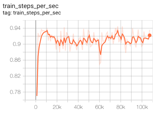
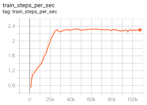
Figure 6. Train steps per second plot for our CT run and the CT run available in the CT repository for Ariane.

H. Are the resources used to run Circuit Training good enough to reproduce the Nature result?

We believe the answer is Yes. We refer to the ISPD-2022 paper by Google authors S. Yu, E. Songhori, W. Jiang, T. Boyd, A. Goldie, A. Mirhoseini and S. Guadarrama, “Scalability and Generalization of Circuit Training for Chip Floorplanning” [YuSJBGMG-ISPD22].

• Training server. In [YuSJBGMG-ISPD22], the authors state: “We think the 8-GPU setup is able to produce better results primarily because it uses a global batch size of 1024, which makes learning more stable and reduces the noise of the policy gradient estimator. Therefore, we recommend using the full batch size suggested in our open-source framework [2] in order to achieve optimal results.”

• Circuit Training (CT, ) itself shows the use of an 8-GPU setup to reproduce their published Ariane results [link].

• We use eight NVIDIA-V100 GPUs to train the model for global batch size = 1024. The global batch size used in the Nature paper (MirhoseiniGYJSWLJPNPTSHTLLHCD21, ) and the global batch size used in our runs are the same (i.e., global batch size = 1024). (MirhoseiniGYJSWLJPNPTSHTLLHCD21, ) refers to the use of 16 GPUs. However, based on the statements given in [YuSJBGMG-ISPD22], and what Circuit Training describes for “Reproduce results”, the final proxy cost achieved by our environment should not differ materially from the environment with 16 GPUs described in (MirhoseiniGYJSWLJPNPTSHTLLHCD21, ).

• Collect servers. Again in [YuSJBGMG-ISPD22], the Google authors state: “With distributed collection, the user can run many (10s-1000s) Actor workers with each collecting experience for a given policy, speeding up the data collection process.” and, “As mentioned in Section 2.2, data collection and multi-GPU training in our framework are independent processes which can be optimized separately.”

• We use two collect servers each running 13 collect jobs, i.e., a total of 26 collect jobs are used for data collection. By contrast, the Nature authors run 512 collect jobs for data collection. The number of collect servers used to run 512 collect jobs is not clear from the description given in the Nature paper. We expect our runtimes to be higher than what Nature reports – and we account for this in our experiments.

• Train steps per second is the indicator of the CT training speed. In Figure 6, the left plot indicates the CT training speed for Ariane in our environment, i.e.,  0.9 steps/second. The right plot indicates the CT training speed for Ariane that is posted in the CT repo, i.e.,  2.3 steps/second. From this we infer that our runtime is expected to be  2.6x times larger than the runtime when the suggested resource (mentioned in the CT repo) is used.

• To make sure that we give the proper amount of resources to Circuit Training in our experiments, we observe from Google’s published Tensorboard that training of Ariane took 14 hours. We therefore give 14 * 2.6 =  36 hours to our Circuit Training environment. (This corresponds to 200 iterations, and this is the number of iterations that we uniformly give to Circuit Training in our experiments.)