Learning Physical Models that Can Respect Conservation Laws

Abstract

Recent work in scientific machine learning (SciML) has focused on incorporating partial differential equation (PDE) information into the learning process. Much of this work has focused on relatively “easy” PDE operators (e.g., elliptic and parabolic), with less emphasis on relatively “hard” PDE operators (e.g., hyperbolic). Within numerical PDEs, the latter problem class requires control of a type of volume element or conservation constraint, which is known to be challenging. Delivering on the promise of SciML requires seamlessly incorporating both types of problems into the learning process. To address this issue, we propose ProbConserv, a framework for incorporating conservation constraints into a generic SciML architecture. To do so, ProbConserv combines the integral form of a conservation law with a Bayesian update. We provide a detailed analysis of ProbConserv on learning with the Generalized Porous Medium Equation (GPME), a widely-applicable parameterized family of PDEs that illustrates the qualitative properties of both easier and harder PDEs. ProbConserv is effective for easy GPME variants, performing well with state-of-the-art competitors; and for harder GPME variants it outperforms other approaches that do not guarantee volume conservation. ProbConserv seamlessly enforces physical conservation constraints, maintains probabilistic uncertainty quantification (UQ), and deals well with shocks and heteroscedasticities. In each case, it achieves superior predictive performance on downstream tasks.

Keywords: scientific machine learning; conservation laws; physically constrained machine learning; partial differential equations; uncertainty quantification; shock location detection

1 Introduction

Conservation laws are ubiquitous in science and engineering, where they are used to model physical phenomena ranging from heat transfer to wave propagation to fluid flow dynamics, and beyond. These laws can be expressed in two complementary ways: in a differential form; or in an integral form. They are most commonly expressed as partial differential equations (PDEs) in a differential form,

$$u_{t}+\nabla\cdot F(u)=0,$$

for an unknown $u$ and a nonlinear flux function $F(u)$. This differential form of the conservation law can be integrated over a spatial domain $\Omega$ using the divergence theorem to result in an integral form of the conservation law,

$$U_{t}=-\int_{\Gamma}F(u)\cdot nd\Gamma,$$

where $U=\int_{\Omega}u(t,x)d\Omega$, $\Gamma$ denotes the boundary of $\Omega$ and $n$ denotes the outward unit normal vector. As examples: in the case of heat transfer, $u$ denotes the temperature, and $U$ the conserved energy of system; and in the case of porous media flow, $u$ denotes the density, and $U$ the conserved mass of the porous media.

Global conservation states that the rate of change in time of the conserved quantity $U$ over a domain $\Omega$ is given by the flux across the boundary $\Gamma$ of the domain. Local conservation arises naturally in the numerical solution of PDEs. Traditional numerical methods (e.g., finite differences, finite elements, and finite volume methods) have been developed to solve PDEs numerically, with finite volume methods being designed for (and being particularly well-suited for) conservation laws (LeVeque, 1990, 2002, 2007). Finite volume methods divide the domain $\Omega$ into control volumes and apply the integral form locally. They enforce that the time derivative of the cell-averaged unknown is equal to the difference between the in-flux and out-flux over the control volume. (This local conservation—so-called since the out-flux that leaves one cell equals the in-flux that enters a neighboring cell—can be used to guarantee global conservation over the whole domain.) This numerical approach should be contrasted with finite difference methods, which use the differential form directly, and which are thus not guaranteed to satisfy the conservation condition.

This discussion is relevant for machine learning (ML) since there has been an interest recently in Scientific ML (SciML) in incorporating the physical knowledge or physical constraints into neural network (NN) training. A popular example of this is the so-called Physics-Informed Neural Networks (PINNs) (Raissi et al., 2019). This approach uses a NN to approximate the PDE solution by incorporating the differential form of the PDE into the loss function, basically as a soft constraint or regularization term. Other data-driven approaches, including DeepONet (Lu et al., 2021) and Neural Operators (NOs) (Li et al., 2021a; Gupta et al., 2021), train on simulations and aim to learn the underlying function map from initial conditions or PDE coefficients to the solution. Other methods such as Physics-Informed Neural Operator (PINO) attempt to make the data-driven Fourier Neural Operator (FNO) “physics-informed,” again by adding the differential form into the supervised loss function as a soft constraint regularization term (Li et al., 2021b; Goswami et al., 2022).

Challenges and limitations for SciML of this soft constraint approach on model training were recently identified (Krishnapriyan et al., 2021; Edwards, 2022). The basic issue is that, unlike numerical finite volume methods, these ML and SciML methods do not guarantee that the physical property of conservation is satisfied. This is a consequence of the fact that the Lagrange dual form of the constrained optimization problem does not in general satisfy the constraint. This results in very weak control on the physical conservation property, resulting in non-physical solutions that violate the governing conservation law.

In this work, we frame the problem of learning physical models that can respect conservation laws via a “finite-volume lens” from scientific computing. This permits us to use the integral form of the governing conservation law to enforce conservation conditions for a range of SciML problems. In particular, for a wide range of initial and boundary conditions, we can express the integral form as a time-varying linear constraint that is compatible with existing ML pipelines. This permits us to propose a two-step framework. In the first step, we use an ML model with a mean and variance estimate to compute a predictive distribution for the solution at specified target points. Possible methods for this step include: classic estimation methods (e.g., Gaussian Processes (Rasmussen & Williams, 2006)); methods designed to exploit the complementary strengths of classical methods and NN methods (e.g., Neural Processes (Kim et al., 2019)); as well as computing ensembles of NN models (to compute empirical estimates of means and variances). In the second step, we apply a discretization of the integral form of the constraint as a Bayesian update in order to enforce the physical conservation constraint on the black-box unconstrained output. We illustrate our framework, ProbConserv, by using an Attentive Neural Process (ANP) (Kim et al., 2019) as the probabilistic deep learning model in the first step paired with a global conservation constraint in the second step. In more detail, the following are our main contributions:

• Integral form for conservation. We propose to use the integral form of the governing conservation law via finite volume methods, rather than the commonly used differential form, to enforce conservation subject to a specified noise parameter. Through an ablation study, we show that adding the differential form of the PDE as a soft constraint to the loss function does not enforce conservation in the underlying unconstrained ML model.

• Strong control on the conservation constraint. By using the integral form, we are able to enforce conservation via linear probabilistic constraints, which can be made arbitrarily binding or sharp by reducing the variance term $\sigma_{G}^{2}$. In particular, by adjusting $\sigma_{G}^{2}$, one can balance satisfying conservation with predictive metrics (e.g., MSE), with ProbConserv obtaining exact conservation when $\sigma_{G}^{2}=0$.

• Effective for “easy” to “hard” PDEs. We evaluate on a parametric family of PDEs, which permits us to explore “easy" parameter regimes as well as “medium" and “hard" parameter regimes. We find that our method and the baselines do well for “easy” problems (although baselines sometimes have issues even with “easy” problems, and even for “easy” problems their solutions may not be conservative), but we do seamlessly better as we go to “harder” problems, with a $5\times$ improvement in MSE.

• Uncertainty Quantification (UQ) and downstream tasks. We provide theoretical guarantees that ProbConserv increases predictive log-likelihood (LL) compared to the original black-box ML model. Empirically, we show that ProbConserv consistently improves LL, which takes into account both prediction accuracy and well-calibrated uncertainty. On “hard” problems, this improved control on uncertainty leads to better insights on downstream shock position detection tasks.

There is a large body of related work, too much to summarize here; see Appendix A for a summary.

2 A Probabilistic Approach to Conservation Law Enforcement

In this section, we present our framework, ProbConserv, for learning physical models that can respect conservation laws. Our approach centers around the following two sources of information: an unconstrained ML algorithm that makes mean and variance predictions; and a conservation constraint (in the form of Equation 4 below) that comes from knowledge of the underlying physical system. See Algorithm 1 for details of our approach. In the first step, we compute a set of mean and variance estimates for the unconstrained model. In the second step, we use those mean and variance estimates to compute an update that respects the conservation law. The update rule has a natural probabilistic interpretation in terms of uncertainty quantification, and it can be used to satisfy the conservation constraint to a user-specified tolerance level. As this tolerance goes to zero, our method gracefully converges to a limiting solution that satisfies conservation exactly (see Theorem 1 below).

  Input: Constraint matrix $G$, constraint value $b$, non-zero noise $\sigma_{G}$ and input points $(t_{1},x_{1}),\dots(t_{N},x_{N})$

  Step 1: Calculate black-box prediction over output grid: ${\mu,\Sigma=f_{\theta}((t_{1},x_{1}),\dots(t_{N},x_{N});D)}$

  Step 2: Calculate $\tilde{\mu}$ and $\tilde{\Sigma}$ according to Equation 8.

  Output: $\tilde{\mu},\tilde{\Sigma}$

Algorithm 1 ProbConserv 

2.1 Integral Form of Conservation Laws as a Linear Constraint

Here, we first derive the integral form of a governing conservation law from the corresponding differential form (a la finite volume methods), and we then show how this integral form can be expressed as a linear constraint (for PDEs with specific initial and boundary conditions, even for certain nonlinear differential PDE operators) for a broad class of real-world problems.

Consider the differential form of the governing equation:

$$\begin{drcases}&\mathcal{F}u(t,x)=0,\,\,x\in\Omega,\\ &u(0,x)=h(x),\,\,x\in\Omega,\\ &u(t,x)=g(t,x),\,\,x\in\Gamma,\end{drcases},\forall\,t\geq 0,$$ (1)

where $\Gamma$ denotes the boundary of the domain $\Omega$, $h(x)$ the initial condition, and $g(t,x)$ the Dirichlet boundary condition. Recently popular SciML methods, e.g., PINNs (Raissi et al., 2019), PINOs (Li et al., 2021b; Goswami et al., 2022), focus on incorporating this form of the constraint into the NN training procedure. In particular, the differential form of the PDE $\mathcal{F}u(t,x)$ could be added as a soft constraint to the loss function $\mathcal{L}$, as follows:

$$\min_{\theta}\mathcal{L}(u)+\lambda\|\mathcal{F}u\|,$$

where $\mathcal{L}$ denotes a loss function measuring the error of the NN approximated solution relative to the known initial and boundary conditions (and potentially any observed solution samples), $\theta$ denotes the NN parameters, and $\lambda$ denotes a penalty or regularization parameter.

For conservation laws, the differential form is given as:

$$\mathcal{F}u=u_{t}+\nabla\cdot F(u),$$ (2)

for some given nonlinear flux function $F(u)$. The corresponding integral form of a conservation law is given as:

$$\int_{\Omega}u(t,x)d\Omega=\int_{\Omega}h(x)d\Omega-\int_{0}^{t}\int_{\Gamma}F(u)\cdot nd\Gamma dt.$$ (3)

See Appendix B for a derivation.

In one-dimension, the boundary integral of the flux can be computed analytically, as the difference of the flux in and out of the domain:

$$\underbrace{\int_{\Omega}u(t,x)d\Omega}_{\mathcal{G}u(t,x)}=\underbrace{\int_{\Omega}h(x)d\Omega+\int_{0}^{t}(F_{\text{in}}-F_{\text{out}})dt}_{b(t)},$$ (4)

where $\Omega=[x_{0},x_{N}]$, $F_{\text{in}}=F(u,t,x_{0})|_{u=g(t,x_{0})}$, and $F_{\text{out}}=F(u,t,x_{N})|_{u=g(t,x_{N})}$. In two and higher dimensions, we do not have an analytic expression, but one can approximate this boundary integral as the sum over the spatial dimensions of the difference of the in and out fluxes on the boundary in that dimension. This methodology is well-developed within finite volume discretization methods, and we leave this extension to future work.

In many applications (including those we consider), by using the prescribed physical boundary condition $u(t,x)=g(t,x)$ for $x\in\Gamma$, it holds that the in and out fluxes on the boundary do not depend on $u$, and instead they only depend on $t$. This is known as a boundary flux linearity assumption since, when it holds, one can use a simple linear constraint to enforce the conservation law. This assumption holds for a broad class of problems—even including nonlinear conservation laws with nonlinear PDE operators $\mathcal{F}$ (See Appendix C for the initial/boundary conditions, exact solutions, exact linear global conservation constraints and Table 5 for a summary). In these cases, Equation 4 results in the following linear constraint equation:

$$\mathcal{G}u(t,x)=\int_{\Omega}u(t,x)d\Omega=b(t),$$ (5)

which can be used to enforce global conservation. See Appendix D.1 for details on how this integral equation can be discretized into a matrix equation.

In other applications, of course, the flux linearity assumption along the boundary of the domain will not hold. For example, the flux may not be known and/or the boundary condition may depend on $u(t,x)$. In these cases, we will not be able to not apply Equation 5 directly. However, nonlinear least squares methods may still be used to enforce the conservation constraint. This methodology is also well-developed, and we leave this extension to future work.

2.2 Step 1: Unconstrained Probability Distribution

In Step 1 of ProbConserv, we use a supervised black-box ML model to infer the mean $\mu$ and covariance $\Sigma$ of the unknown function $u$ from observed data $D$. For example, $D$ can include values of the function $u$ observed at a small set of points. Over a set of $N$ input points $(t_{1},x_{1}),\dots,(t_{N},x_{N})$, the probability distribution of $u\coloneqq[u(t_{1},x_{1}),\dots u(t_{N},x_{N})]\in\mathbb{R}^{N}$ conditioned on data $D$ has mean ${\mu\coloneqq\mathbb{E}(u|D)}$ and covariance ${\Sigma\coloneqq\text{Cov}(u|D)}$ given by the black-box model $f_{\theta}$, i.e.,

$$\mu,\Sigma=f_{\theta}\left((t_{1},x_{1}),\dots,(t_{N},x_{N});D\right).$$ (6)

This framework is general, and there are possible choices for the model in Equation 6. Gaussian Processes (Rasmussen & Williams, 2006) are a natural choice, assuming that one has chosen an appropriate mean and kernel function for the specific problem. The ANP model (Kim et al., 2019), which uses a transformer architecture to encode the mean and covariance, is another choice. A third option is to perform repeated runs, e.g., with different initial seeds, of non-probabilistic black-box NN models to compute empirical estimates of mean and variance parameters.

2.3 Step 2: Enforcing Conservation Constraint

In Step 2 of ProbConserv, we incorporate a discretized and probabilistic form of the constraint given in Equation 5:

$$\begin{split}b&=Gu+\sigma_{G}\epsilon,\end{split}$$ (7)

where $G$ denotes a matrix approximating the linear operator $\mathcal{G}$ (see Appendix D.1), $b$ denotes a vector of observed constraint values, and $\epsilon$ denotes a noise term, where each component has unit variance. The parameter $\sigma_{G}\geq 0$ controls how much the conservation constraint can be violated (see Appendix E for details), with $\sigma_{G}=0$ enforcing exact adherence. Step 2 outputs the following updated mean $\tilde{\mu}$ and covariance $\tilde{\Sigma}$ that respect conservation, given as:

$$\tilde{\mu} =\mu-\Sigma G^{T}(\sigma_{G}^{2}I+G\Sigma G^{T})^{-1}(G\mu-b),$$ (8a)

$$\tilde{\Sigma} =\Sigma-\Sigma G^{T}(\sigma_{G}^{2}I+G\Sigma G^{T})^{-1}G\Sigma,$$ (8b)

where $\mu$ and $\Sigma$ denote the mean and covariance matrix, respectively, from Step 1 (Equation 6).

The update rule given in Equation 8 can be justified from two complementary perspectives. From a Bayesian probabilistic perspective, Equation 8 is the posterior mean and covariance of the predictive distribution of $u$ after incorporating the information given by the conservation constraint via Equation 7. From an optimization perspective, Equation 8 is the solution to a least-squares problem that places a binding inequality constraint on the conserved quantity $G\tilde{\mu}$ (i.e., $\|G\tilde{\mu}-b\|_{2}\leq c$ for some ${c\in(0,\|G\mu-b\|_{2})}$). See Appendix F for more details on these two complementary perspectives.

We emphasize that, for $\sigma_{G}>0$, the final solution does not satisfy $G\tilde{\mu}=b$ exactly. Adherence to the constraint can be gracefully controlled by shrinking $\sigma_{G}$. Specifically, if we consider a monotonic decreasing sequence of constraint values $\sigma_{G,n}\downarrow 0$, then the corresponding sequence of posterior means $\tilde{\mu}_{n}$ is well-behaved, and the limiting solution can be calculated. This is shown in the following theorem.

Theorem 1

Let $\mu$ and $\Sigma$ be the mean and covariance of $u$ obtained at the end of Step 1. Let $\sigma_{G,n}\downarrow 0$ be a monotonic decreasing sequence of constraint values and let $\tilde{\mu}_{n}$ be the corresponding posterior mean at the end of Step 2 shown in Equation 8. Then:

1. The sequence $\tilde{\mu}_{n}$ converges to a limit $\tilde{\mu}^{\star}$ monotonically; i.e., $\|\tilde{\mu}_{n}-\tilde{\mu}^{\star}\|_{\Sigma^{-1}}\downarrow 0$.

2. The limiting mean $\tilde{\mu}^{\star}$ is the solution to a constrained least-squares problem: $\mathrm{argmin}_{y}\|y-\mu\|_{\Sigma^{-1}}$ subject to $Gy=b$.

3. The sequence $G\tilde{\mu}_{n}$ converges to $b$ in $L_{2}$; i.e., $\|G\tilde{\mu}_{n}-b\|_{2}\downarrow 0$.

Moreover, if the conservation constraint $Gu=b$ holds exactly for the true solution $u$, then:

1. The distance between the true solution $u$ and the posterior mean $\tilde{\mu}_{n}$ decreases as $\sigma_{G,n}\to 0$, i.e., ${\|\tilde{\mu}_{n}-u\|_{\Sigma^{-1}}\downarrow\|\tilde{\mu}^{\star}-u\|_{\Sigma^{-1}}}$.

2. For sufficiently small $\sigma_{G,n}$, the log-likelihood $\text{LL}(u;\tilde{\mu}_{n},\tilde{\Sigma}_{n})$ is greater than $\text{LL}(u;\mu,\Sigma)$ and increases as $\sigma_{G,n}\to 0$.

See Appendix G for a proof of Theorem 1. Importantly, Theorem 1 holds for any mean and covariance estimates $\mu,\Sigma$, whether they come from a Gaussian Process, ANP, or repeated runs of a black-box NN. It also shows that we are guaranteed to improve in log-likelihood (LL), which we also verify in the empirical results (see Appendix E).

We should also emphasize that, in addition to conservation, Equation 7 can incorporate other inductive biases, based on knowledge of the underlying PDE. To take but one practically-useful example, one typically desires a solution that is free of artificial high-frequency oscillations. This smoothing can be accomplished by penalizing large absolute values of the second derivative via a second order central finite difference discretization in the matrix $\tilde{G}$ (see Appendix D.2).

3 Empirical Results

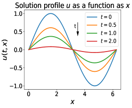
(a) easy: Diffusion equation ($k=1$)

(b) medium: PME ($k(u)=u^{3}$)

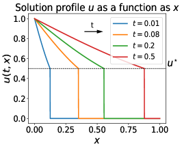
(c) hard: Stefan (discont. $k(u)$)

Figure 1: Illustration of the “easy-to-hard” paradigm for PDEs, for the GPME family of conservation equations: (a) “easy” parabolic smooth (diffusion equation) solutions, with constant parameter $k(u)=k\equiv 1$; (b) “medium” degenerate parabolic PME solutions, with nonlinear monomial coefficient $k(u)=u^{m}$, with parameter $m=3$ here; and (c) “hard” hyperbolic-like (degenerate parabolic) sharp solutions (Stefan equation) with nonlinear step-function coefficient $k(u)=\bm{1}_{u\geq u^{\star}}$, where $\bm{1}_{\mathcal{E}}$ is an indicator function for event $\mathcal{E}$.

In this section, we provide an empirical evaluation to illustrate the main aspects of our proposed framework ProbConserv. We choose the ANP model (Kim et al., 2019) as our black-box, data-driven model in Step 1, and we refer to this instantiation of our framework as ProbConserv-ANP. Unless otherwise stated, we use the limiting solution described in Equation 8, with $\sigma_{G}=0$, so that conservation is enforced exactly through the integral form of the PDE. We organize our empirical results around the following questions:

1. Integral vs. differential form?

2. Strong control on the enforcement of the conservation constraint?

3. “Easy” to “hard” PDEs?

4. Uncertainty Quantification (UQ) for downstream tasks?

Generalized Porous Medium Equation.

The parametric Generalized Porous Medium Equation (GPME) is a family of conservation equations, parameterized by a nonlinear coefficient $k(u)$. It has been used in applications ranging from underground flow transport to nonlinear heat transfer to water desalination and beyond (Vázquez, 2007). The GPME is given as:

$$u_{t}-\nabla\cdot(k(u)\nabla u)=0,$$ (9)

where $F(u)=-k(u)\nabla u$ is a nonlinear flux function, and where the parameter $k=k(u)$ can be varied. Even though the GPME is nonlinear in general, for specific initial and boundary conditions, it has closed form self-similar solutions (Vázquez, 2007; Maddix et al., 2018a, b). This enables ease of evaluation by comparing each competing method to ground truth solutions.

By varying the parameter $k(u)$ in the GPME family, one can obtain PDE problems with widely-varying difficulties, from “easy” (where finite element and finite difference methods perform well) to “hard” (where finite volume methods are needed), and exhibiting many of the qualitative properties of smooth/easy parabolic to sharp/hard hyperbolic PDEs. See Figure 1 for an illustration. In particular: the Diffusion equation is parabolic, linear and smooth, and represents an “easy” case (Sec. 3.1); the Porous Medium Equation (PME) has a solution that becomes sharper (as $m\geq 1$, for $k(u)=u^{m}$, increases), and represents an “intermediate” or “medium” case (Sec. 3.2); and the Stefan equation has a solution that becomes discontinuous, and represents a “hard” case (Sec. 3.3).

We consider these three instances of the GPME (Diffusion, PME, Stefan) that represent increasing levels of difficulty. In particular, the challenging Stefan test case illustrates the importance of developing methods that satisfy conservation conditions on “hard” problems, with non-smooth and even discontinuous solutions, as well as for downstream tasks, e.g., the estimation of the shock position over time. This is important, given the well-known inductive bias that many ML methods have toward smooth/continuous behavior.

See Appendix H for more on the GPME; see Appendix I for details on the ProbConserv-ANP model schematic (Figure 7), model training, data generation and the ANP; and see Appendix J for additional empirical results on the GPME and hyperbolic conservation laws.

Baselines.

We compare our results to the following baselines:

• ANP: Base unconstrained ANP (Kim et al., 2019), trained to minimize the negative evidence lower bound (ELBO):

  $$\mathcal{L}=-\mathbb{E}_{D,u\sim p}\mathbb{E}_{z\sim q_{\phi}}\log p_{\theta}(u,z|D)-\log q_{\phi}(z|u,D),$$

  where $q_{\phi}$ denotes the variational distribution of the data used for training, and $p_{\theta}$ denotes the generative model. The ANP learns a global latent representation $z$ that captures uncertainty in global parameters, which influences the prediction of the reference solution $u$. At inference time, the distribution of $u$ given $z$ ($p_{\theta}(u|z,D)$) outputs a mean and diagonal covariance for Step 1.

• SoftC-ANP: In this “Physics-Informed” Neural Process ablation, we include a soft constrained PDE in the loss function, as is done with PINNs (Raissi et al., 2019), to obtain:

  $$\mathcal{L}+\lambda\mathbb{E}_{z\sim q_{\phi}}\|\mathcal{F}\mu_{z}\|_{2}^{2},$$

  where $\mathcal{F}$ denotes the underlying PDE differential form in Equation 1, $\mu_{z}$ denotes the output mean of the ANP, and $\lambda$ denotes a hyperparameter controlling the relative strength of the penalty. (See Appendix J.1.2 for details on the hyperparameter tuning of $\lambda$.)

• HardC-ANP: In this hard-constrained Neural Process ablation, we project the ANP mean to the nearest solution in $L_{2}$ satisfying the integral form of conservation constraint. This method is inspired by the approach taken in Négiar et al. (2023) that projects the output of a neural network onto the nearest solution satisfying a linear PDE system. HardC-ANP is an alternative to Step 2 that solves the following constrained least-squares problem:

  $$\mu_{HC} =\mathrm{argmin}_{u}\|u-\mu\|_{2}^{2}~{}\text{s.t.}~{}Gu=b$$

  $$=\mu-G^{T}(GG^{T})^{-1}(G\mu-b).$$

  HardC-ANP is equivalent to the limiting solution of the mean of ProbConserv as $\sigma_{G}\to 0$ in Equation 8a, if the variance from Step 1 is fixed to be the same for each point, i.e., $\Sigma=I$.

Evaluation.

At test time, we select a value of the PDE parameter $\alpha$ that lies within the range of PDE parameters used during training (i.e., $\alpha\in\mathcal{A}$). For each value of $\alpha$, we generate multiple independent draws of $(D_{i},u_{i},b_{i})$ in the same manner as the training data. For a given prediction of the mean $\mu$ and covariance $\Sigma$ at a particular time-index $t_{j}$ in the training window, we report the following prediction metrics: conservation error $(\text{CE}(\mu)=(G\mu-b)_{t_{j}}$); predictive log-likelihood $(\text{LL}(u;\mu,\Sigma)={-\frac{1}{2M}\|u_{t_{j},\cdot}-\mu_{t_{j},\cdot}\|_{\Sigma^{-1}_{t_{j}}}-\frac{1}{2M}\sum_{i}\log\sigma^{2}_{t_{j},i}-\log 2\pi})$; and mean-squared error $(\text{MSE}(u,\mu)=\frac{1}{M}\|u_{t_{j},\cdot}-\mu_{t_{j},\cdot}\|^{2}_{2})$, where $M$ denotes the number of spatial points and $\sigma^{2}_{t_{j},\cdot}$ denotes the diagonal of $\Sigma_{t_{j}}\in\mathbb{R}^{M\times M}$. We report the average of each metric over $n_{\text{test}}=50$ independent runs. Our convention for bolding the CE metric is binary on whether conservation is satisfied exactly or not. For the LL and MSE metrics, we bold the methods whose mean metric is within one standard deviation of the best mean metric.

3.1 Diffusion Equation: Constant $k$

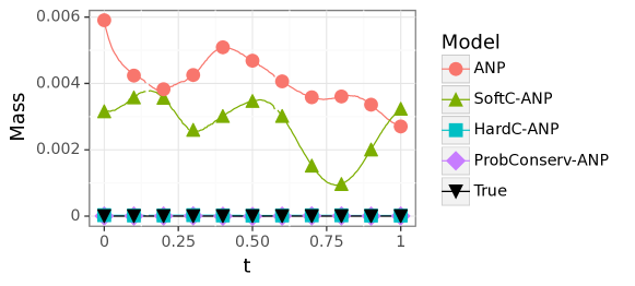
Figure 2: The total mass $U(t)=\int_{\Omega}u(t,x)d\Omega$ as a function of time $t$ for the (“easy”) diffusion equation with constant diffusivity coefficient $k\in\mathcal{A}=[1,5]$ and test-time parameter value $k=1$. The true $U(t)$ is zero at all times since there is zero net flux from the domain boundaries and mass cannot be created or destroyed on the interior. Both ProbConserv-ANP and HardC-ANP satisfy conservation of mass exactly. The other baselines violate conservation and result in a non-physical mass profile over time. ANP and SoftC-ANP are not even zero at time $t=0$.

The diffusion equation is the simplest non-trivial form of the GPME, with constant diffusivity coefficient $k(u)=k>0$ (see Figure 1(a)). We train on values of $k\in\mathcal{A}=[1,5]$. The diffusion equation is also known as the heat equation, where in that application the PDE parameter $k$ denotes the conductivity and the total conserved quantity denotes the energy. In our empirical evaluations, we use the diffusion equation notation, and refer to the conserved quantity as the mass.

Table 1: Mean and standard error for CE $\times 10^{-3}$ (should be zero), LL (higher is better) and MSE $\times 10^{-4}$ (lower is better) over $n_{\text{test}}=50$ runs for the (“easy") diffusion equation at time $t=0.5$ with variable diffusivity constant $k$ parameter in the range $\mathcal{A}=[1,5]$ and test-time parameter value $k=1$.

	CE	LL	MSE
ANP	4.68 (0.10)	$2.72$ (0.02)	$1.71$ (0.41)
SoftC-ANP	3.47 (0.17)	$2.40$ (0.02)	$2.24$ (0.78)
HardC-ANP	0 (0.00)	3.08 (0.04)	$\mathbf{1.37}$ (0.33)
ProbConserv-ANP	0 (0.00)	2.74 (0.02)	1.55 (0.33)

Figure 2 illustrates that the unconstrained ANP solution violates conservation by allowing mass to enter and exit the system over time. Physically, there is no in-flux or out-flux on the boundary of the domain, and thus the true total mass of the system $U(t)=\int_{\Omega}u(t,x)d\Omega$ is zero at all times. Surprisingly, even incorporating the differential form of the conservation law as a soft constraint into the training loss via SoftC-ANP violates conservation and the violation occurs even at $t=0$.

Enforcing conservation as a hard constraint in our ProbConserv-ANP model and HardC-ANP guarantees that the system total mass is zero, and also leads to improved predictive performance for both methods. In particular, Table 1 shows that these methods exactly obtain the lowest MSE and the highest LL. The success of these two approaches that enforce the integral form of the conservation law exactly, along with the failure of SoftC-ANP that penalizes the differential form, demonstrates that physical knowledge must be properly incorporated into the learning process to improve predictive accuracy. Figure 9 in Appendix J.1.1 illustrates that these conservative methods perform well on this “easy” case since the uncertainty from the ANP is relatively homoscedastic throughout the solution space; that is, the estimated errors are mostly the same size, and the constant variance assumption in HardC-ANP holds reasonably well.

Table 2: Mean and standard error for CE $\times 10^{-3}$ (should be zero), LL (higher is better) and MSE $\times 10^{-4}$ (lower is better) over $n_{\text{test}}=50$ runs for the (“medium”) PME at time $t=0.5$ with variable $m$ parameter in the range $\mathcal{A}=[0.99,6]$. For test-time parameter $m=1$, where conservation by the unconstrained ANP is violated the most, ProbConserv-ANP leads to a substantial $\mathbf{5.5\times}$ improvement in MSE and log-likelihood. For test-time parameters $m=3,6$, the MSE for ProbConserv-ANP increases due to the error concentrated at the sharper boundary while the desired log-likelihood and conservation metrics improve.

	$m=1$			$m=3$			$m=6$
	CE	LL	MSE	CE	LL	MSE	CE	LL	MSE
ANP	$6.67$ (0.39)	$3.49$ (0.01)	$0.94$ (0.09)	$-1.23$ (0.29)	$3.67$ (0.00)	$1.90$ (0.04)	$-2.58$ (0.23)	$3.81$ (0.01)	7.67 (0.09)
SoftC-ANP	$5.62$ (0.35)	$3.11$ (0.01)	$1.11$ (0.14)	$-0.65$ (0.30)	$3.46$ (0.00)	$2.06$ (0.03)	$-3.03$ (0.26)	$3.49$ (0.00)	$7.82$ (0.09)
HardC-ANP	0 (0.00)	3.16 (0.04)	0.43 (0.04)	0 (0.00)	$3.44$ (0.03)	1.86 (0.03)	0 (0.00)	3.40 (0.05)	7.61 (0.09)
ProbConserv-ANP	0 (0.00)	3.56 (0.01)	0.17 (0.02)	0 (0.00)	3.68 (0.00)	2.10 (0.07)	0 (0.00)	3.83 (0.01)	10.4 (0.04)

3.2 Porous Medium Equation (PME): $k(u)=u^{m}$

The Porous Medium Equation (PME) is a subclass of the GPME in which the coefficient, $k(u)=u^{m},$ is nonlinear and smooth (see Figure 1(b)). The PME is known to be degenerate parabolic, with different behaviors depending on the value of $m$. We train on values of $m\in\mathcal{A}=[0.99,6]$.

Table 2 compares the CE, MSE, and LL results for $m=1,3,6$. These three values of $m$ reflect “easy,” “medium,” and “hard” scenarios, respectively, as the solution profile becomes sharper. Despite achieving relatively low MSE for $m=1$, the ANP model violates conservation the most. The error profiles as a function of $x$ in Figure 11 in Appendix J.1.2 illustrate the cause: the ANP consistently overestimates the solution to the left of the shock. Enforcing conservation consistently fixes this bias, leading to errors that are distributed around $0$. Our ProbConserv-ANP method results in an $\approx 82\%$ improvement in MSE, and HardC-ANP results in an $\approx 54\%$ improvement over the ANP. Since HardC-ANP shifts every point equally, it induces a negative bias in the zero (degeneracy) region of the domain, leading to a non-physical solution.

For $m=3,6$, while the MSE for ProbConserv-ANP increases compared to the ANP, the LL for ProbConserv-ANP improves. The increase in LL for ProbConserv-ANP indicates that the uncertainty is better calibrated as a whole. Figure 11 in Appendix J.1.2 illustrates that ProbConserv-ANP reduces the errors to the left of the shock point while increasing the error immediately to the right of it. This error increase is penalized more in the $L_{2}$ norm, which leads to an increase in MSE. The LL metric improves because our ProbConserv-ANP model takes into account the estimated variance at each point. It is expected that the largest uncertainty occurs at the sharpest part of the solution, since that is the area with the largest gradient. This region is more difficult to be captured as the shock interface becomes sharper when $m$ is increased.

For control on the enforcement of conservation constraint, see Figure 5 in Appendix E, where we show empirically that the log likelihood is always increasing, as stated in Theorem 1. Note that there are optimal values of $\sigma_{G}^{2}$, in which case the MSE can be better optimized.

3.3 Stefan Problem: Discontinuous Nonlinear $k(u)$

Table 3: Mean and standard error for CE $\times 10^{-2}$ (should be zero), LL (higher is better), and MSE $\times 10^{-3}$ (lower is better) over $n_{\text{test}}=50$ runs for the (“hard”) Stefan variant of the GPME at time $t=0.05$. Each model is trained with the parameter $u^{\star}$ in the range $\mathcal{A}=[0.55,0.7]$ and test-time parameter value $u^{\star}=0.6$. ProbConserv-ANP leads to an increase in log-likelihood and a $\mathbf{3\times}$ decrease in MSE.

	CE	LL	MSE
ANP	-1.30 (0.01)	3.53 (0.00)	5.38 (0.01)
SoftC-ANP	-1.72 (0.04)	3.57 (0.01)	6.81 (0.15)
HardC-ANP	0 (0.00)	2.33 (0.06)	5.18 (0.02)
ProbConserv-ANP	0 (0.00)	3.56 (0.00)	1.89 (0.01)

The most challenging case of the GPME is the Stefan problem. In this case, the coefficient $k(u)$ is a discontinuous nonlinear step function $k(u)=\bm{1}_{u\geq u^{\star}}$, where $\bm{1}_{\mathcal{E}}$ denotes an indicator function for event _E and $u^{\star}\in\mathbb{R}_{+}$. The solution is degenerate parabolic and develops a moving shock over time (see Figure 1(c)). We train on values of $u^{\star}\in\mathcal{A}=[0.55,0.7]$ and evaluate the predictive performances of each model at $u^{\star}=0.6$.

Unlike the PME test case, where the degeneracy point ($x^{*}(t)=t$) is the same for each value of $m$, the shock position for the Stefan problem depends on the parameter $u^{\star}$ (See Figure 4 in Appendix C). This makes the problem more challenging for the ANP, as it can no longer memorize the shock position. On this “harder” problem, the unconstrained ANP violates the physical property of conservation by an order of magnitude larger in CE than in the “easier” diffusion and PME cases. By enforcing conservation of mass, ProbConserv-ANP results in substantial $\approx 65\%$ improvement in MSE (Table 3). In addition, Figure 3(a) shows that the solution profiles associated with ANP and the other baselines are smoothed and deviate more from the true solution than the solution profile of our ProbConserv-ANP model. Similar to our previous two case studies, adding the differential form of the PDE via SoftC-ANP does not lead to a conservative solution (see Figure 12 in Appendix 12). In fact, Table 3 shows that surprisingly, conservation is violated more by SoftC-ANP than with the ANP, with a corresponding increase in MSE. These results demonstrate that physics-based constraints, e.g., conservation laws need be incorporated carefully (via finite volume based ideas) into ML-based models.

Table 3 shows that the LL for ProbConserv-ANP increases only slightly, compared to that of the ANP (3.56 vs 3.53), and it is slightly less than SoftC-ANP. Figure 3(a) shows that enforcing conservation of mass creates a small upward bias in the left part of the solution profile for $x\in[0,0.2]$. Since the variance coming from the ANP is smaller in that region, this bias is heavily penalized in the LL. This bias is worse for HardC-ANP, which assumes an identity covariance matrix and ignores the uncertainty estimates from the ANP. HardC-ANP adds more noticeable upward bias to the $x\in[0,0.2]$ region, and it even adds bias to the zero-density region to the right of the shock. Compared to ProbConserv-ANP, HardC-ANP only leads to a slight reduction in MSE (3%) and a much lower LL (2.33). This shows the benefit of using the uncertainty quantification from the ANP in our ProbConserv-ANP model for this challenging heteroscedastic case.

Downstream Task: Shock Point Estimation.

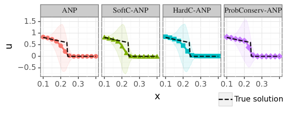
(a) Solution profile.

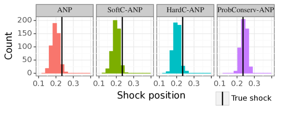
(b) Posterior of the shock position.

Figure 3: (a) Stefan solution profiles at time $t=0.05$ with training parameter values $u^{\star}\in\mathcal{A}=[0.55,0.7]$ and test-time parameter $u^{\star}=0.6$. ProbConserv-ANP results in a sharper solution profile and the solution is mean-centered around the shock position. (b) The corresponding histogram of the posterior of the shock position computed as the mean plus or minus 3 standard deviations. ProbConserv-ANP reduces the level of underestimation and the induced negative bias at the shock interface to result in more accurate shock position prediction.

While quantifying predictive performance in terms of MSE or LL is useful in ML, these metrics are typically not of direct interest to practitioners. To this end, we consider the downstream task of shock point estimation, which is an important problem in fluids, climate, and other areas. The shock position for the Stefan problem $x^{\star}(t)$ depends on the parameter $u^{\star}$. Hence, for a given function at test-time, the shock position $x^{\star}(t)$ is unknown and must be predicted from the estimated solution profile.

We define the shock point at time $t$ as the first spatial point (left-to-right) where the function equals zero:

$$x^{\star}(t)=\inf_{x}\{u(t,x)=0\}.$$ (10)

On a discrete grid, we approximate the infimum using the minimum. The advantage of a probabilistic approach is that we can directly quantify the uncertainty of $x^{\star}(t)$ by drawing samples from the posterior distributions of our ProbConserv-ANP model and the baselines.

Figure 3(b) shows the corresponding histograms of the posterior of the shock position. We see that our ProbConserv-ANP posterior is centered around the true shock value. By underestimating the solution profile, the ANP misses the true shock position wide to the left, as do the other baselines SoftC-ANP and HardC-ANP. Remarkably, neither adding the differential form as a soft constraint (SoftC-ANP) nor projecting to the nearest conservative solution in $L_{2}$ (HardC-ANP) helps with the task of shock position estimation. This result highlights that both capturing the physical conservation constraint and using statistical uncertainty estimates in our ProbConserv-ANP model are necessary on challenging problems with shocks, especially when the shock position is unknown.

4 Conclusion

We have formulated the problem of learning physical models that can respect conservation laws from the finite volume perspective, by writing the governing conservation law in integral form rather than the commonly-used (in SciML) differential form. This permits us to incorporate the global integral form of the conservation law as a linear constraint into black-box ML models; and this in turn permits us to develop a two-step framework that first trains a black-box probabilistic ML model, and then constrains the output using a probabilistic constraint of the linear integral form. Our approach leads to improvements (in MSE, LL, etc.) for a range of “easy” to “hard” parameterized PDE problems. Perhaps more interestingly, our unique approach of using uncertainty quantification to enforce physical constraints leads to improvements in challenging shock point estimation problems. Future extensions include support for local conservation in finite volume methods, where the same linear constraint approach can be taken by computing the fluxes as latent variables; imposing boundary conditions as linear constraints (Saad et al., 2023); and extension to other physical constraints, including nonlinear constraints, e.g., enstrophy in 2D and helicity in 3D, and inequality constraints, e.g., entropy (Tezaur et al., 2017).

Appendix A Related Works

Our method involves combining in a novel way ideas from several different literatures. As such, there is a large body of related work, each of which approaches the problems we consider from somewhat different perspectives. Here, we summarize some of the most related. Table 4 provides an overview of the comparisons of these methods.

Table 4: Summary of different properties of numerical and SciML methods for physical systems.

Method	Conservative	UQ	Inference with different Initial Conditions	Inference with different PDE coefficients	Resolution independent
Numerical methods	✓	✗	✗	✗	✗
PINNs	✗	✗	✗	✗	✓
Neural Operators	✗	✗	✓	✓	✓
Conservative ML models	✓	✗	✓	✗	✗
ProbConserv (our approach)	✓	✓	✓	✓	✓

A.1 Numerical Methods

Numerical methods aim to approximate the solution to partial differential equations (PDEs) by first discretizing the spatial domain $\Omega$ into $N$ gridpoints $\{x_{i}\}_{i=1}^{N}$ with spatial step size $\Delta x$. Then, at each time step, we integrate the resulting semi-discrete ODE in time with temporal step size $\Delta t$ to iteratively compute the solution at final time $T$, i.e., $\{u(T,x_{i})\}_{i=1}^{N}$. By the Lax Equivalence theorem for linear problems, convergence to the true solution, i.e., the norm of the error tending to zero, can be proven to occur when $\Delta t,\Delta x\rightarrow 0$ ($N\rightarrow\infty$) for methods that are both stable and consistent (LeVeque, 2007). A limitation of numerical methods is that to obtain higher accuracy, fine mesh resolutions must be used, which can be computationally expensive in higher dimensions. In addition, for changes in PDE parameters, the simulations need to be re-run. These classical methods are also deterministic, and they do not provide uncertainty quantification.

Finite Volume Methods.

Finite volume methods are designed for conservation laws. These methods divide the domain into control volumes, where the integral form of the governing equation is solved (LeVeque, 1990, 2002). By solving the integral form at each control volume, these methods enforce flux continuity, i.e., that the out-flux of one cell is equal to the in-flux of its neighbor. This results in local conservation, which guarantees global conservation over the entire domain. Maddix et al. (2018a) show that the degenerate parabolic Generalized Porous Medium Equation (GPME) has presented challenges for classical averaged-based finite volume methods, e.g., arithmetic and harmonic averaging. These numerical artifacts include artificial temporal oscillations, and locking or lagging of the shock position. To eliminate these artifacts on the more challenging Stefan problem, Maddix et al. (2018b) show that information about the shock location needs to be incorporated into the scheme to satisfy the Rankine-Hugoniot condition. Other complex methods that explicitly track the front, e.g., front-tracking methods (Al-Rawahi & Tryggvason, 2002; Li et al., 2003) and level set methods (Osher & Sethian, 1988) that implicitly model the interface as a signed distance function, have also been applied to the Stefan problem for modeling crystallization (Sethian & Strain, 1992; Chen et al., 1997).

Reduced Order Models (ROMs).

Reduced Order Models (ROMs) have been a popular alternative to full order model numerical PDE simulations for computational efficiency. ROMs aim to approximate the solution in a lower dimensional subspace by computing the proper orthogonal decomposition (POD) basis using the singular value decomposition (SVD). Similar to deep learning models, there is no way to enforce that unconstrained ROMs are conservative and non-oscillatory. Tezaur et al. (2017) investigate enforcing conservative, entropy and total variation diminishing (TVD) constraints for ROMs as constrained nonlinear least squares problems. These methods are coined “structure preserving” ROMs via physics-based constraints (Sargsyan, 2016).

A.2 Scientific Machine Learning (SciML) Models

Here we describe the recent work in using ML models to solve PDEs. At a high-level, these works can be divided into three categories: 1. Physics-Informed Neural Networks (PINNs), which aim to incorporate PDE information as a soft constraint in the loss function; 2. Neural Operators, which aim to learn the solution mapping from PDE coefficients or initial conditions to solutions; and 3. Hard-constrained conservative ML models, which aim to incorporate different types of constraints to enforce conservation into the architecture.

Physics-informed ML Methods.

Physics-informed neural networks (PINNs) (Raissi et al., 2019) parameterize the solution to PDEs with a neural network (NN). These methods impose physical knowledge into neural networks by adding the differential form of the PDE to the loss function as a soft constraint or regularizer. Purely data-driven approaches include DeepONet (Lu et al., 2021) and Neural Operators (NOs) (Li et al., 2020, 2021a; Gupta et al., 2021), which aim to learn the underlying function map from initial conditions or PDE coefficients to the solution. Learning this mapping enables these methods to be resolution independent, i.e., train on a coarse resolution and perform inference on a finer resolution. These methods only use PDE knowledge implicitly by training on simulations. The Physics-Informed Neural Operator (PINO) attempts to address that the physics are not directly enforced in the model by making the data-driven Fourier Neural Operator (FNO) “physics-informed.” To do so, they again add the differential form into the supervised loss function as a soft constraint regularization term (Li et al., 2021b; Goswami et al., 2022).

Recently Krishnapriyan et al. (2021); Edwards (2022) identified several challenges and limitations for SciML of this soft constraint approach on the training procedure for several PDEs with large parameter values. In particular, Krishnapriyan et al. (2021) show that the sharp and non-smooth loss surface created by adding the PDE directly as a regularizer can be more difficult to optimize. Relatedly, PINO has been shown to perform worse than the base FNO without the differential form of the PDE as a soft constraint in the loss (Li et al., 2021b; Saad et al., 2023). Motivated by these observations, Négiar et al. (2023) propose a solution for linear PDEs that enforces the differential form of the PDE as a hard constraint; and Subramanian et al. (2022) propose another solution using an adaptive update of collocation points. In addition, Wang et al. (2022) examine training issues associated with the spectral bias in PINNs (Jacot et al., 2018). Edwards (2022) discusses the broader-scale impacts of these results for the SciML field, and motivates the need for better solutions that capture the underlying continuous physics.

Machine Learning Models for Conservation Laws.

Enforcing the PDE as a soft constraint gives very weak control on the physical conservation property, resulting in non-physical solutions that can violate governing conservation law. Jekel et al. (2022) aim to satisfy conservation by adding the continuity equation as a soft regularizer via the PINNs approach, and they show that this does not improve performance. To try to remedy this, Mao et al. (2020); Jagtap et al. (2020) propose conservative PINNs (cPINNs) for conservation laws, which aim to enforce flux continuity, i.e., the out-flux of one cell equals the in-flux of the neighboring cell, for a type of local conservation. Again, however, this condition on the flux is added to the loss function as a regularization term, i.e., as a soft constraint in a Lagrange dual form, and so the conservation condition is in general not exactly satisfied.

Motivated by the importance of satisfying conservation laws in climate applications, Bolton & Zanna (2019); Zanna & Bolton (2020); Beucler et al. (2021) have proposed building known linear physical constraints directly into deep learning architectures. Beucler et al. (2021) propose a model that forces the output of a neural network into the null space of the constraint matrix. While the solution exactly satisfies the constraints, the constraints depend on the resolution of the data, and they are an approximation to the true physical quantity that needs to be constrained. Surprisingly, Beucler et al. (2021) also finds that the reconstruction error is not always improved with adding constraints. Other methods to enforce conservation include the following. Sturm & Wexler (2022) enforce the flux continuity equation in the last layer of the neural network to model the balance of atoms. Müller (2022) enforce conservation by encoding symmetries using Noether’s theorem. Richter-Powell et al. (2022) propose so-called Neural Conservation Laws, to enforce conservation by design by using parametizations of deep neural networks similar to the approaches in Négiar et al. (2023); Sturm & Wexler (2022); Müller (2022). In particular, Richter-Powell et al. (2022) use a change of variables that combines time and space derivatives into the divergence operator to create a divergence-free model, and they then use auto-differentiation similar to the Neural ODEs approach (Chen et al., 2018). This optimize-then-discretize approach has been shown to have related difficulties (Krishnapriyan et al., 2022; Ott et al., 2021; Onken & Ruthotto, 2020).

Appendix B Derivation of the Integral Form of a Conservation Law

To obtain the integral form of a conservation law, given in Equation 3 as:

$$\int_{\Omega}u(t,x)d\Omega=\int_{\Omega}h(x)d\Omega-\int_{0}^{t}\int_{\Gamma}F(u)\cdot nd\Gamma dt,$$ (11)

we first integrate the differential form of the conservation law, given in Equation 2 as:

$$\mathcal{F}u=u_{t}+\nabla\cdot F(u),$$ (12)

over the spatial domain $\Omega$. From this, we obtain an expression for the rate of change in time of the total conserved quantity in terms of the fluxes on the boundary, given as:

$$\frac{d}{dt}\int_{\Omega}u(t,x)d\Omega =\int_{\Omega}u_{t}(t,x)d\Omega$$ (13a)

$$=-\int_{\Omega}\nabla\cdot F(u)d\Omega$$ (13b)

$$=-\int_{\Gamma}(F(u)\cdot n)d\Gamma,$$ (13c)

where the last step is obtained by applying the divergence theorem to the flux term, and $n$ is the outward pointing unit normal on the boundary $\Gamma$.

We then integrate Equation 13 over the temporal domain $[0,t]$. Doing this to Equation 13a yields:

$$\int_{0}^{t}\int_{\Omega}u_{t}(t,x)d\Omega=\int_{\Omega}u(t,x)d\Omega-\int_{\Omega}u(0,x)d\Omega,$$

where $u(0,x)=h(x)$ denotes the initial condition. By equating this quantity to the temporal integral of the right hand side of Equation 13c, we obtain the corresponding integral form of a conservation law:

$$\int_{\Omega}u(t,x)d\Omega=\int_{\Omega}h(x)d\Omega-\int_{0}^{t}\int_{\Gamma}F(u)\cdot nd\Gamma dt,$$

which is Equation 11.

Appendix C Exact Solutions and Linear Conservation Constraints for Conservation Laws

In this section, we provide the exact solutions to a wide range of conservation laws:

$$\begin{drcases}&\underbrace{u_{t}+\nabla\cdot F(u)}_{\mathcal{F}u}=0,\,\,x\in\Omega,\\ &u(0,x)=h(x),\\ &u(t,x)=g(t,x),\,\,x\in\Gamma,\end{drcases},\forall\,t\geq 0,$$ (14)

for general nonlinear flux $F(u)$, nonlinear differential operator $\mathcal{F}$, initial condition $h(x)$ and prescribed boundary conditions on the boundary $\Gamma$ of the spatial domain $\Omega$. These exact solutions are used to generate the solution samples for the training data in the experiment section 3.

The integral form of the conservation law in Equation 4 is given as:

$$\underbrace{\int_{\Omega}u(t,x)d\Omega}_{\mathcal{G}u(t,x)}=\underbrace{\int_{\Omega}h(x)d\Omega+\int_{0}^{t}(F_{\text{in}}-F_{\text{out}})dt}_{b(t)},$$ (15)

where $\Omega=[x_{0},x_{N}]$, $F_{\text{in}}=F(u,t,x_{0})|_{u=g(t,x_{0})}$, $F_{\text{out}}=F(u,t,x_{N})|_{u=g(t,x_{N})}$ and $g(t,x)$ is the prescribed Dirichlet boundary condition in Equation 14. We provide the exact formulation of our linear constraint $\mathcal{G}u(t,x)=b(t)$. Table 5 provides a summary, showing that our boundary flux linearity assumption holds for a broad class of problems—even including nonlinear conservation laws with nonlinear PDE operators $\mathcal{F}$.

Table 5: Classification of PDE conservation laws ranging from “easy” to “hard”, and corresponding total time-varying conserved value $b(t)$ in the integral form of Equation 15 for specified flux function $F(u)$, initial and boundary conditions $h(x)$ and $g(t,x)$, respectively in Equation 14. See Section C.1.3 for the value of the constant $c_{1}\in\mathbb{R}$.

PDE	Type	$F(u)$	$h(x)$	$g(t,x)$	$\Omega$	$\Gamma$	$b(t)$
Diffusion	Linear parabolic (“easy”)	$-k\nabla u$, $k\in\mathbb{R}_{+}$	$\sin(x)$	$\{0,0\}$	$[0,2\pi]$	$\{0,2\pi\}$	$0$
PME	Nonlinear degenerate parabolic (“medium”)	$-u^{m}\nabla u$, $m\in\mathbb{Z}_{+}$	0	$\{(mt)^{1/m},0\}$	$[0,1]$	$\{0,1\}$	$\frac{m^{1+1/m}}{m+1}t^{1+1/m}$
Stefan	Nonlinear degenerate parabolic (“hard”)	$\begin{dcases}-\nabla u,\hskip 2.84544ptu\geq u^{\star}\\ 0,\hskip 2.84544pt\text{otherwise}\end{dcases}$, $u^{\star}\in\mathbb{R}_{+}$	$0$	$\{1,0\}$	$[0,1]$	$\{0,1\}$	$2c_{1}\sqrt{t/\pi}$
Advection	Linear hyperbolic (“medium”)	$\beta u$, $\beta\in\mathbb{R}_{+}$	$\begin{dcases}1,\hskip 2.84544ptx\leq 0.5\\ 0,\hskip 2.84544pt\text{otherwise}\end{dcases}$	$\{1,0\}$	$[0,1]$	$\{0,1\}$	$\frac{1}{2}+\beta t$
Burgers’	Nonlinear hyperbolic (“hard”)	$\frac{1}{2}u^{2}$	$\begin{dcases}-ax,\hskip 2.84544ptx\leq 0,a\in\mathbb{R}_{+}\\ 0,\hskip 2.84544pt\text{otherwise}\end{dcases}$	$\{a,0\}$	$[-1,1]$	$\{-1,1\}$	$(a/2)(1+at)$

C.1 GPME Family of Conservation Laws

In this subsection, we consider the (degenerate) parabolic GPME family of conservation laws given in Equation 9 as:

$$u_{t}-\nabla\cdot(k(u)\nabla u)=0,$$

with flux $F(u)=-k(u)\nabla u$. Figure 4 shows the effects of the various PDE parameters $k(u)$ at a fixed time $t$ on the solution on three instances of the GPME ranging from the “easy” to “hard” cases, i.e., the diffusion equation, PME and Stefan, respectively.

(a) $k$: Diffusion equation at $t=1$ (“easy”).

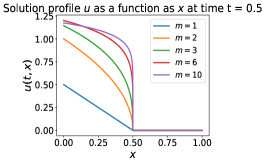
(b) $m$: PME at $t=0.5$ (“medium”).

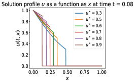
(c) $u^{\star}$: Stefan at $t=0.08$ (“hard”).

Figure 4: Effect of PDE parameters on the three “easy” to “hard” instances of the GPME at fixed time $t$.

C.1.1 Diffusion Equation

The heat or diffusion equation is a simple linear parabolic PDE with constant coefficient $k(u)=k$, which represents an “easy” task. Figure 4(a) illustrates the effect of the constant diffusivity (conductivity) parameter $k$ on solutions to the diffusion (heat) equation. For larger values of $k$, we see that the solution more quickly dissipates toward the constant smooth zero steady state.

Exact Solution.

We use the same diffusion test problem from Krishnapriyan et al. (2021) with the following initial condition and periodic boundary conditions:

$$u(0,x) =h(x)=\sin(x),\forall x\in\Omega=[0,2\pi],$$

$$u(t,0) =u(t,2\pi),\forall t\ \in[0,T],$$

respectively. The exact solution is given as

$$u(t,x)=FT^{-1}(FT(h(x))e^{-kn^{2}t}),$$

where $FT$ denotes the Fourier transform, and $n$ denotes the frequency in the Fourier domain.

Global Conservation.

The total mass (energy) is constant and zero over all time, since there is no in or out flux to the domain. Then, Equation 15 reduces to the following linear homogeneous system:

$$\mathcal{G}u(t,x)=\int_{x_{0}}^{x_{N}}u(t,x)dx=0=b(t).$$ (16)

To derive the above relation, we see by using separation of variables that the solution $u(t,x)=\sin(x)T(t)$ is a damped sine curve over time. The flux $F(u)=-k\nabla u=-\cos(x)T(t)$, where $T(t)$ denotes a decaying exponential function. Then, the integral form in Equation 15 is given as:

$$\int_{\Omega}u(t,x)d\Omega =\int_{\Omega}h(x)d\Omega+\int_{0}^{t}[F(u,t,x_{0}=0)-F(u,t,x_{N}=2\pi)]dt$$

$$=\int_{0}^{2\pi}\sin(x)d\Omega-k\int_{0}^{t}[\cos(0)T(t)-\cos(2\pi)T(t)]dt=0,$$

by periodicity.

C.1.2 Porous Medium Equation

In the Porous Medium Equation (PME), the nonlinearity and small values of the coefficient $k(u)=u^{m}$, for $m\geq 1$, cause challenges for current state-of-the-art SciML baselines as well as classical numerical methods on this degenerate parabolic equation. The difficulty increases as the exponent $m$ increases, and the solution forms sharper corners. In particular, the solution gradient is finite for $m=1$, and it approaches infinity near the front for $m>1$. Figure 4(b) illustrates the effect of the parameter $m$ on the solution, with solutions for $m>1$ being sharper, and having a different profile than those for the piecewise linear solution for $m=1$.

Exact Solution.

We test the locking problem (TLP) of the PME from Lipnikov et al. (2016); Maddix et al. (2018a) with the following initial and growing in time Dirichlet left boundary conditions for some final time $T\leq 1$:

$$u(0,x) =h(x)=0,\forall x\in\Omega=[0,1],$$

$$u(t,0) =g(t,0)=(mt)^{1/m},\forall t\in[0,T],$$

$$u(t,1) =g(t,1)=0,\forall t\in[0,T],$$

respectively. The exact solution is given as:

$$u(t,x)=(m(t-x)_{+})^{1/m}.$$ (17)

Global Conservation.

We write the specific form of the linear conservation constraint in Equation 15 for the PME as:

$$\mathcal{G}u(t,x)=\int_{x_{0}}^{x_{N}}u(t,x)dx=\frac{m^{1+1/m}}{m+1}t{{}^{1+1/m}}=b(t),$$ (18)

by using the fact that the total mass of the initial condition is zero, and that $u(t,x_{N}=1)=0$ on the right boundary for $t\leq x_{N}=1$.

Global conservation is driven by the in-flux at the growing in left boundary, where

$$F_{\text{in}}=F(u,t,x_{0})|_{u=g(t,x_{0}),x=x_{0}}=-g(t,x_{0})^{m}\nabla u|_{x=x_{0}}=-mt\nabla u|_{x=x_{0}}.$$

The boundary flux at the right boundary is 0, since we assume that the shock is contained in the domain and $t>x$, hence $u(t,1)=0$ and

$$F_{\text{out}}=F(u,t,x_{N})|_{u=g(t,x_{N}),x=x_{N}}=-g(t,x_{N})^{m}\nabla u|_{x=x_{N}}=0.$$

The first integral on the righthand side in Equation 15 consisting of the initial mass is 0, since $h(x)=0$, and we are left only with the in-flux term:

$$\int_{\Omega}u(t,x)d\Omega =\int_{0}^{t}F_{\text{in}}(t)dt$$

$$=-\int_{0}^{t}g(t,x_{0}=0)^{m}\nabla u|_{x=x_{0}}dt$$

$$=\int_{0}^{t}(mt)(mt)^{1/m-1}dt$$

$$=m^{1/m}\int_{0}^{t}t^{1/m}dt$$

$$=\frac{m^{1+1/m}}{m+1}t^{1+1/m},$$

where $\nabla u|_{x=x_{0}}=-(m(t-x))^{1/m-1}|_{x=x_{0}}=-(mt)^{1/m-1}$.

C.1.3 Stefan Problem

The Stefan problem is the most challenging problem in the GPME degenerate parabolic family of conservation equations since the coefficient $k(u)$ is a nonlinear step function of the unknown $u$, given as:

$$k(u)=\begin{cases}k_{\max},\hskip 2.84544ptu\geq u^{\star},\\ k_{\min},\hskip 2.84544ptu<u^{\star},\end{cases}$$ (19)

for constants $k_{\max},k_{\min}\in\mathbb{R}$ and $u(t,x^{*}(t))=u^{*}\in\mathbb{R}_{+}$ for shock position $x^{*}(t)$. In this problem, the solution is a shock or moving interface with a finite speed of propagation that does not dissipate over time. Figure 4(c) illustrates the effect of the parameter $u^{\star}$ on the solution and shock position, with smaller values of $u^{\star}$ resulting in a faster shock speed.

Exact Solution.

We use the Stefan test case from van der Meer et al. (2016); Maddix et al. (2018b) with $k_{\max}=1$, $k_{\min}=0$ in Equation 19, and the following initial and Dirichlet boundary conditions for some final time $T$:

$$u(0,x) =h(x)=0,\forall x\in\Omega=[0,1],$$

$$u(t,0) =g(t,0)=1,\forall t\in[0,T],$$

$$u(t,1) =g(t,1)=0,\forall t\in[0,T],$$

respectively. The exact solution is given as:

$$u(t,x)=\bm{1}_{u\geq u^{\star}}\left(1-c_{1}\Phi[x/(2\sqrt{k_{\text{max}}t})]\right),$$ (20)

where $\bm{1}_{\mathcal{E}}$ denotes an indicator function for event $\mathcal{E}$, $\Phi(x)=\text{erf}(x)=\int_{0}^{x}\phi(y)dy$ denotes the error function with $\phi(y)=(2/\sqrt{\pi})\exp(-y^{2})$, and constant $c_{1}=(1-u^{*})/\Phi[\alpha/(2\sqrt{k_{\max}})]$. A nonlinear solve for $\tilde{\alpha}$: $(1-u^{*})/\sqrt{\pi}=u^{*}\Phi(\tilde{\alpha})\tilde{\alpha}\exp(\tilde{\alpha}^{2})$, is used to compute $\alpha=2\sqrt{k_{\max}}\tilde{\alpha}$. The exact shock position is $x^{*}(t)=\alpha\sqrt{t}$.

Global Conservation.

We write the linear $\mathcal{G}$ conservation constraint in Equation 15 for the Stefan equation as:

$$\mathcal{G}u(t,x)=\int_{x_{0}}^{x_{N}}u(t,x)dx=2c_{1}\sqrt{\frac{k_{\max}t}{\pi}}=b(t).$$ (21)

We use the fact that the solution is monotonically non-increasing to compute the coefficient values at the boundaries, i.e., $u(t,x_{0})\geq u^{\star}\geq u(t,x_{N})$, where $0=x_{0}\leq x^{\star}\leq x_{N}=1$ and $x^{*}(t)$ denotes the shock position. It follows that $k(u(t,x_{0}))=k_{\max}$ and $k(u(t,x_{N}))=0$. Then the out-flux $F_{\text{out}}=k(u(t,x_{N}))\nabla u=0$. The first integral on the righthand side of Equation 15 consisting of the initial mass is 0, since $h(x)=0$, and we are left only with the in-flux term as follows:

$$\int_{\Omega}u(t,x)d\Omega =\int_{0}^{t}F_{\text{in}}(t)dt$$

$$=-k_{\max}\int_{0}^{t}\nabla u|_{x=x_{0}}dt$$

$$=c_{1}\sqrt{\frac{k_{\max}}{\pi}}\int_{0}^{t}t^{-1/2}dt$$

$$=2c_{1}\sqrt{\frac{k_{\max}t}{\pi}},$$

where $\nabla u|_{x=x_{0}}=-c_{1}\Phi^{\prime}[x_{0}/(2\sqrt{k_{\max}}t)]/(2\sqrt{k_{\max}}t)=-c_{1}/\sqrt{\pi k_{\max}t}\exp[x_{0}^{2}/(4k_{\max}t)]=-c_{1}/\sqrt{\pi k_{\max}t}$ for $x_{0}=0$.

C.2 Hyperbolic Conservation Laws

In this section, we consider hyperbolic conservation laws, where solutions exhibit shocks and smooth initial conditions self-sharpen over time (LeVeque, 1990, 2002).

C.2.1 Linear Advection

The linear advection (convection) equation:

$$u_{t}+\beta u_{x}=0,$$ (22)

is a hyperbolic conservation law with flux $F(u)=\beta u$, where a fluid with density $u$ is transported or advected by some constant velocity $\beta\in\mathbb{R}$. For larger values of $\beta$, the shock moves faster.

Exact Solution.

Here we consider the test case with the following initial and boundary conditions:

$$u(0,x) =h(x)=\bm{1}_{x\leq 0.5},\forall x\in\Omega=[0,1],$$

$$u(t,0) =g(t,0)=1,\forall t\in[0,T],$$

$$u(t,1) =g(t,1)=0,\forall t\in[0,T],$$

respectively, and $\bm{1}_{\mathcal{E}}$ denotes an indicator function for event $\mathcal{E}$. Note that the linear advection (convection) problem is also studied in Krishnapriyan et al. (2021) with smooth $h(x)=\sin(x)$ and periodic boundary conditions. Here we consider the more challenging case, where the initial condition is already a shock.

In our case, the exact solution,

$$u(t,x)=h(x-\beta t),$$

is simply the initial condition shifted to the right, which is a shock wave traveling to the right with speed $\beta>0$.

Global Conservation.

We write the linear conservation constraint in Equation 15 for linear advection as:

$$\mathcal{G}u(t,x)=\int_{x_{0}}^{x_{N}}u(t,x)dx=\frac{1}{2}+\beta t=b(t).$$ (23)

The out-flux $F_{\text{out}}=u(t,1)=g(t,1)=0$, by the fixed right Dirichlet boundary condition, and we are left with the following terms:

$$\int_{\Omega}u(t,x)d\Omega =\int_{\Omega}h(x)dx+\int_{0}^{t}F_{\text{in}}(t)dt$$

$$=\int_{0}^{0.5}dx+\beta\int_{0}^{t}u(t,0)dt$$

$$=\frac{1}{2}+\beta t,$$

by using the Dirichlet boundary condition $u(t,0)=g(t,0)=1$ in the second term in the last step. We see that the time rate of change in total mass is constant over time.

C.2.2 Burgers’ Equation

Burgers’ Equation, given as:

$$u_{t}+\frac{1}{2}(u^{2})_{x}=0,$$ (24)

is a commonly used nonlinear hyperbolic conservation law with flux $F(u)=\frac{1}{2}u^{2}$. Among other things, it is used in traffic modeling.

Exact Solution.

We consider the test case from Tezaur et al. (2017), where $a=1$, with the following initial and boundary conditions:

$$u(0,x) =h(x)=\begin{cases}a,\hskip 2.84544ptx\leq-1,\\ -ax,\hskip 2.84544pt-1\leq x\leq 0,\\ 0,\hskip 2.84544ptx\geq 0,\end{cases}\forall x\in\Omega=[-1,1],$$

$$u(t,-1) =g(t,-1)=a,\forall t\in[0,T],$$

$$u(t,1) =g(t,1)=0,\forall t\in[0,T],$$

respectively for constant, positive parameter slope $a\geq 1$. For larger values of $a$, the slope of the initial condition is steeper, and a shock is formed faster.

We write the nonlinear Burgers’ Equation 24 in non-conservative form as

$$u_{t}+uu_{x}=0.$$

We see that this is the advection Equation 22 with speed $\beta=u$. Hence, similarly the exact solution is given by $u(t,x)=h(x-ut)$ when the characteristics curves do not intersect, by using the method of characteristics (Evans, 2010). We then obtain the following solution:

$$u(t,x)=\begin{cases}a,\hskip 2.84544ptx-ut\leq-1,\\ -a(x-ut),\hskip 2.84544pt-1\leq x-ut\leq 0,\\ 0,\hskip 2.84544ptx-ut\geq 0.\end{cases}$$

We use the second case to solve this implicit equation explicitly for $u$, i.e., $u=-a(x-ut)\iff u=\frac{-ax}{1-at}$. Then $x-ut=\frac{x}{1-at}$, where the denominator $1-at>0$ for $t<1/a$. We then solve the inequalities and substitute this in to obtain:

$$u(t,x)=\begin{cases}a,\hskip 21.33955ptx\leq at-1,\\ \frac{ax}{at-1},\hskip 12.80365ptat-1\leq x\leq 0,\\ 0,\hskip 21.33955ptx\geq 0,\end{cases}$$

for $0\leq t<1/a$. We see that as time increases the linear part of the solution self-sharpens with a steeper slope until the characteristics intersect at breaking time

$$t_{b}=\frac{-1}{\inf_{x}h^{\prime}(x)}=1/a,$$

and a shock is formed. This is known as the waiting time phenomenon (Maddix et al., 2018b). The rightward moving shock forms with weak solution given as:

$$u(t,x)=\begin{cases}a,\hskip 2.84544ptx\leq\frac{1}{2}(at-1),\\ 0,\hskip 2.84544ptx\geq\frac{1}{2}(at-1),\end{cases}$$

for $t\geq 1/a$. The shock speed $x^{\prime}(t)$ is given by the Rankine-Hugoniot (RH) condition (Evans, 2010). The RH condition simplifies for Burgers’ Equation as follows:

$$x^{\prime}(t)=\frac{f(u_{R})-f(u_{L})}{u_{R}-u_{L}}=\frac{1}{2}\frac{u_{R}^{2}-u_{L}^{2}}{u_{R}-u_{L}}=\frac{1}{2}\frac{(u_{R}-u_{L})(u_{R}+u_{L})}{u_{R}-u_{L}}=\frac{u_{R}+u_{L}}{2}=\frac{a}{2},$$

where $u_{L}=a$ denotes the solution value to the left of the shock and $u_{R}=0$ denotes the solution value to the right of the shock. Lastly, to obtain the shock position $x(t)$, we solve the simple ODE $x^{\prime}(t)=a/2$ with initial condition $x(t_{b}=1/a)=0$ to obtain $x(t)=\frac{at}{2}+c$, where $x(1/a)=\frac{1}{2}+c=0$, and so $c=-\frac{1}{2}$. This results in $x(t)=\frac{1}{2}(at-1)$, as desired.

Global Conservation.

We write the linear conservation constraint in Equation 15 for Burgers’ equation as:

$$\mathcal{G}u(t,x)=\int_{x_{0}}^{x_{N}}u(t,x)dx=\frac{a}{2}(1+at)=b(t).$$ (25)

The out-flux is $F_{\text{out}}=\frac{1}{2}u(t,1)^{2}=\frac{1}{2}g(t,1)^{2}=0$, by the fixed right Dirichlet boundary condition, and we are left with the following terms:

$$\int_{\Omega}u(t,x)d\Omega =\int_{\Omega}h(x)dx+\int_{0}^{t}F_{\text{in}}(t)dt$$

$$=-a\int_{-1}^{0}xdx+\frac{1}{2}\int_{0}^{t}u(t,-1)^{2}dt$$

$$=\frac{a}{2}(1+at),$$

by using the Dirichlet boundary condition $u(t,-1)=g(t,-1)=a$ in the second term in the last step. We again see that the time rate of change in total mass is constant over time.

Appendix D Discretizations of the Integral Operator $\mathcal{G}$ for Conservation and Additional Linear Constraints

In this section, we first describe common discretization schemes $G$ for the integral operator $\mathcal{G}$ in Equation 5 given as:

$$\mathcal{G}u(t,x)=\int_{\Omega}u(t,x)d\Omega=b(t),$$ (26)

to form a linear matrix constraint equation $Gu=b$. Then, we show how to incorporate other types of linear constraints into our framework ProbConserv. In particular, we consider artificial diffusion, which is a common numerical technique to smooth numerical artifacts through the matrix $\tilde{G}$ arising from the second order central finite difference scheme of the second derivative.

D.1 Discretizations of the Integral Operator $\mathcal{G}$

Here, we provide examples of the discrete matrix $G\in\mathbb{R}^{T\times MT}$, which approximates the continuous integral operator $\mathcal{G}$ in Equation 26. We use $M$ to denote the number of spatial points, $T$ to denote the number of time points, and we set $N=MT$.

We form a discrete linear system from the continuous integral conservation law, i.e,. $Gu=b$, where each row $i$ of $G$ acts as a Riemann approximation to the integral $\mathcal{G}u(t,x)$ at time $t_{i}$. At inference time, we assume we have an ordered output grid $\{(t_{1},x_{1}),\dots,(t_{1},x_{M}),\dots,(t_{T},x_{1}),\dots,(t_{T},x_{M})\}$ with spatial grid spacing $\Delta x_{j}=x_{j+1}-x_{j}$ for $j=1,\dots,M-1$. We want to compute the solution at these corresponding grid points given as:

$$u=[u(t_{1},x_{1}),\dots,u(t_{1},x_{M}),\dots,u(t_{T},x_{1}),\dots,u(t_{T},x_{M})]^{T}\in\mathbb{R}^{MT}.$$

The known right-hand side is given as:

$$b=[b(t_{1}),\dots,b(t_{T})]^{T}\in\mathbb{R}^{T}.$$

We now proceed to provide examples of specific matrices $G$ corresponding to common numerical spatial integration schemes (Burden et al., 2016).

Left Riemann Sum.

For $G$ arising from the common first-order left Riemann sum

$$\sum_{j=1}^{M-1}u(t_{i},x_{j})\Delta x_{j},$$

at time $t_{i}$, we have the following expression:

$$G_{ij}=\begin{dcases}\Delta x_{j},\hskip 2.84544pt(i-1)M+1\leq j\leq iM-1,\\ 0,\hskip 2.84544pt\text{otherwise}.\end{dcases}$$

In other words, it uses the left function value $u(t,x_{j})$ on the interval $[x_{j},x_{j+1}]$. The right Riemann sum ($\sum_{j=2}^{M}u(t,x_{j})\Delta x_{j-1}$ at time $t$) is a simple extension that shifts the column indices by 1 to $(i-1)M+2\leq j\leq iM$ to use the right value $u(t_{i},x_{j+1})$ on the interval $[x_{j},x_{j+1}]$.

Trapezoidal Rule.

For $G$ arising from the second order trapezoidal rule

$$Gu=\sum_{j=1}^{M-1}\frac{u(t_{i},x_{j})+u(t_{i},x_{j+1})}{2}\Delta x_{j},$$

at time $t_{i}$, we have the following expression:

$$G_{ij}=\begin{dcases}\frac{\Delta x_{j}}{2},\hskip 2.84544ptj=(i-1)M+1,\\ \frac{\Delta x_{j-1}+\Delta x_{j}}{2},\hskip 2.84544pt(i-1)M+2\leq j\leq iM-1,\\ \frac{\Delta x_{j-1}}{2},\hskip 2.84544ptj=iM,\\ 0,\hskip 2.84544pt\text{otherwise}.\end{dcases}$$ (27)

We use the trapezoidal discretization of $G$ in Equation 27 in our experiments. Note that higher order schemes, e.g., Simpson’s Rule may also be used, as well as more advanced numerical techniques. These can help to reduce the error in the spatial integration approximation, including shock tracking schemes in Maddix et al. (2018b) on the more challenging sharper problems with shocks that we see for high values of $m$ in the PME and Stefan.

D.2 Adding Artificial Diffusion into the Discretization

In addition to various discretization schemes to compute the integral operator $\mathcal{G}$, our ProbConserv framework can incorporate other inductive biases based on the knowledge of the underlying PDE, e.g., to bypass undesirable numerical artifacts. One common technique that has been used widely in numerical methods for this purpose is adding artificial diffusion (Maddix et al., 2018a). This artificial diffusion can act locally at sharp corners such as shock interfaces, where numerical methods tend to suffer from high frequency oscillations. Other common numerical methods to avoid numerical oscillations include total variation diminishing (TVD), i.e., $\text{TV}(u(t_{i+1},x))\leq\text{TV}(u(t_{i},x))$, $\forall i$, or total variation bounded (TVB), i.e., $\text{TV}(u(t_{i+1},x))\leq C$, $C>0$, $\forall i$, where $\text{TV}(u)=\int_{\Omega}|\frac{\partial u}{\partial x}|d\Omega$ and is approximated as $\sum_{j=1}^{M-1}|u(t_{i},x_{j+1})-u(t_{i},x_{j})|$ (LeVeque, 1990; Tezaur et al., 2017). Note that enforcing these inequality constraints is a direction of future work.

In machine learning, artificial diffusion is analogous to adding a regularization penalty on the $L_{2}$ norm of the second derivative $\int\{\frac{\partial^{2}}{\partial x^{2}}u(t_{i},x)\}^{2}dx$ (Hastie et al., 2013). This can be written as the $L_{2}$ norm of a linear operator applied to $u$, $\|\tilde{\mathcal{G}}(u)\|_{2}^{2}$, where $\tilde{\mathcal{G}}(u)(t_{i})\coloneqq\frac{\partial^{2}}{\partial x^{2}}u(t_{i},x)$. Thus, we can incorporate this penalty term into ProbConserv in the same manner as the integral operators by discretizing $\tilde{\mathcal{G}}$ via a matrix $\tilde{G}$. Let $\tilde{G}$ be the second order central finite difference three-point stencil at time $t_{i}$ over $M$ spatial points:

$$\begin{split}(\tilde{G}u)_{j}&=\left(\frac{u(t_{i},x_{j+2})-u(t_{i},x_{j+1})}{\Delta x_{j+1}}\right)-\left(\frac{u(t_{i},x_{j+1})-u(t_{i},x_{j})}{\Delta x_{j}}\right).\\ \end{split}$$

for $j=1,\dots,M-2$. For simplicity of notation, we assume $\Delta x_{j}\coloneqq\Delta x$ for all $x_{j}$, though this need not be the case in general. This results in the following three-banded matrix:

$$\begin{split}\tilde{G}&=\frac{1}{\Delta x}\begin{bmatrix}1&-2&1&0&\dots\\ 0&1&-2&1&\dots\\ \vdots&\vdots&\vdots&\vdots&\vdots\\ \end{bmatrix}.\end{split}$$ (28)

Since our goal is to penalize large differences in the solution, we set the constraint value $b$ to zero:

$$\tilde{G}u+\sigma_{\tilde{G}}\epsilon=0,$$

where $\sigma_{\tilde{G}}>0$ denotes the constraint value for the artificial diffusion. Since the mechanism is exactly the same with a linear constraint, artificial diffusion can be applied using Equation 8a with $b=0$, where $\tilde{\mu}$ and $\tilde{\Sigma}$ are the mean and covariance after applying the conservation constraint as follows:

$$\begin{split}\tilde{\mu}_{\text{diffusion}}&=\tilde{\mu}-\tilde{\Sigma}\tilde{G}^{T}(\sigma^{2}_{\tilde{G}}I+G\tilde{\Sigma}G^{T})^{-1}(\tilde{G}\tilde{\mu}),\\ \tilde{\Sigma}_{\text{diffusion}}&=\tilde{\Sigma}-\tilde{\Sigma}\tilde{G}^{T}(\sigma^{2}_{\tilde{G}}I+G\tilde{\Sigma}G^{T})^{-1}(\tilde{G}\tilde{\Sigma}).\end{split}$$

Moreover, the guarantees of Theorem 1 still hold. Smaller values of $\sigma_{\tilde{G}}$ lead to smaller values of $\|\tilde{G}\tilde{\mu}_{\text{diffusion}}\|_{2}^{2}$, which results in a smoother solution.

Unlike the case of enforcing conservation, it is typically not desirable when applying artificial diffusion to set $\sigma_{\tilde{G}}$ to zero, as this will lead to a simple line fit (Hastie et al., 2013). We set the variance for each row of $\tilde{G}$ as follows: Let $\sigma_{i}^{2}\coloneqq\text{Var}(u_{n})$ be the variance of target value $u_{n}$ from the Step 1 procedure:

$$\sigma_{\tilde{G},i}^{2}\coloneqq\text{Var}((\tilde{G}u)_{i})=\text{Var}(u_{i}-2u_{i+1}+u_{i+2})=\sigma_{i}^{2}+4\sigma_{i+1}^{2}+\sigma_{i+2}^{2}-4\rho\left(\sigma_{i}\sigma_{i+1}+\sigma_{i+1}\sigma_{i+2}\right)+2\rho^{2}\sigma_{i}\sigma_{i+2},$$

where $\rho\in[0,1]$ determines the level of auto-correlation between neighboring points. Higher values of $\rho$ lead to lower values of $\sigma^{2}_{\tilde{G},i}$, and hence a higher penalty.

Appendix E Control on Conservation Constraint

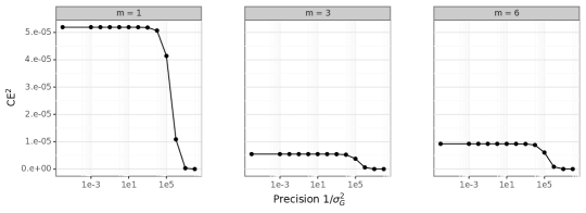
(a) Norm of the conservation error: $\text{CE}^{2}(\tilde{\mu})=\|G\tilde{\mu}-b\|_{2}^{2}$.

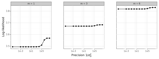
(b) Log-likelihood: $\text{LL}(u;\tilde{\mu},\tilde{\Sigma})={-\frac{1}{2M}\|u_{t_{j},\cdot}-\tilde{\mu}_{t_{j},\cdot}\|_{\tilde{\Sigma}^{-1}_{t_{j}}}-\frac{1}{2M}\sum_{i}\log\tilde{\sigma}^{2}_{t_{j},i}-\log 2\pi}$.

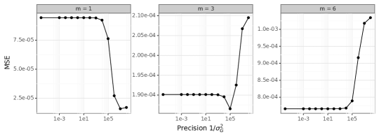
(c) Mean-squared error: $\text{MSE}(u,\tilde{\mu})=\frac{1}{M}\|u_{t_{j},\cdot}-\tilde{\mu}_{t_{j},\cdot}\|^{2}_{2}$.

Figure 5: Illustration of the norm of the conservation error $\text{CE}^{2}$ (lower is better) in the top row, the predictive log likelihood (LL) in the middle row (higher is better), and the mean-squared error (MSE) (lower is better) in the bottom row, as a function of the constraint precision $\frac{1}{\sigma_{G}^{2}}$ for ProbConserv-ANP on the PME in subsection 3.2, where $M$ denotes the number of spatial points, $\tilde{\sigma}^{2}_{t_{j},\cdot}$ denotes the diagonal of the covariance $\tilde{\Sigma}_{t_{j}}\in\mathbb{R}^{M\times M}$ and $t_{j}$ denotes the time-index in the training window at which the metrics are reported. Each column indicates results for a different values of PDE parameter $m\in\{1,3,6\}$, corresponding to “easy”, “medium”, and “hard” scenarios, respectively. In all three cases, $\text{CE}^{2}$ monotonically decreases to zero and LL monotonically increases as $\sigma_{G}^{2}\to 0$ ($1/\sigma_{G}^{2}\rightarrow\infty$), illustrating Theorem 1. The biggest gains in log-likelihood are for $m=1$, where conservation was also violated the most. In contrast, the relationship between MSE and $\frac{1}{\sigma_{G}^{2}}$ is not guaranteed to be monotonic, and it qualitatively changes, depending on the value of $m$.

Figure 5 illustrates that Theorem 1 holds empirically for ProbConserv-ANP on the PME in subsection 3.2, where both the norm of the conservation error ($\text{CE}^{2}$) monotonically decreases to zero and the predictive log likelihood (LL) monotonically increases as the constraint precision $\sigma_{G}^{2}\rightarrow 0$ ($1/\sigma_{G}^{2}\rightarrow\infty$). For the MSE, the trend depends on the difficulty of the problem. For “easy” scenarios, where $m=1$, the MSE also monotonically improves (decreases) as $\sigma_{G}^{2}\rightarrow 0$ ($1/\sigma_{G}^{2}\rightarrow\infty$). For “medium” difficulty problems, where $m=3$, we see that there is an optimal value for $\sigma_{G}^{2}$ around $10^{-5}$, and enforcing the constraint exactly does not result in the lowest MSE. For the “harder” $m=6$ case, we see that a looser tolerance on the constraint results in better MSE. In this case the solution is non-physical since it does not satisfy conservation. Note that in the sharper $m=6$ case, the accuracy may be able to be improved by using more advanced approximations for the integral operator $\mathcal{G}$ that take the sharp corners in the solution into account (Maddix et al., 2018b).

Appendix F Derivation of Constrained Mean and Covariance

In this section, we provide two interpretations for the Step 2 procedure of ProbConserv from Equation 8 given as:

$$\tilde{\mu} =\mu-\Sigma G^{T}(\sigma_{G}^{2}I+G\Sigma G^{T})^{-1}(G\mu-b),$$ (29a)

$$\tilde{\Sigma} =\Sigma-\Sigma G^{T}(\sigma_{G}^{2}I+G\Sigma G^{T})^{-1}G\Sigma.$$ (29b)

While Equation 8 is well-defined in the case that $\sigma_{G}^{2}=0$, for simplicity we assume $\sigma_{G}^{2}>0$ throughout this section. In Lemma 1, we show how Step 2 is justified as a Bayesian update of the unconstrained normal distribution from Step 1 by adding information about the conservation constraint contained in Equation 7, i.e., $b=Gu+\sigma_{G}\epsilon$ in Step 2. In Lemma 2, we show how the posterior mean $\tilde{\mu}$ and $\tilde{\Sigma}$ can be re-expressed in a numerically stable and computationally efficient form given in Equation 29. Finally, Lemma 3 shows that this is equivalent to a least-squares optimization with an upper bound on the conservation error.

Note: $\mu\in\mathbb{R}^{MT},\Sigma\in\mathbb{R}^{MT\times MT},G\in\mathbb{R}^{T\times MT},b\in\mathbb{R}^{T}$, where $N=MT$ denotes the number of spatio-temporal output points, $M$ denotes the number of spatial points and $T$ denotes number of constraints or in this case time steps to enforce the conservation constraint.

Lemma 1 (Step 2 as Bayesian update)

Assume the predictive distribution of $u$ conditioned only on observed data $D$ is normal with mean $\mu$ and covariance $\Sigma$. Let $b$ be the known conservation quantity that follows a normal distribution with mean $Gu$ and covariance $\sigma_{G}^{2}I$, where $\sigma_{G}^{2}>0$. Then the posterior distribution of $u$ conditional on both data $D$ and conservation quantity $b$ is normal with mean $\tilde{\mu}$ and covariance $\tilde{\Sigma}$ given as:

$$\begin{split}u|b,D&\sim\mathcal{N}(\tilde{\mu},\tilde{\Sigma}),\\ \tilde{\Sigma}&=A^{-1}\Sigma,\\ \tilde{\mu}&=A^{-1}(\mu+\frac{1}{\sigma_{G}^{2}}\Sigma G^{T}b),\end{split}$$

where $A=I+\frac{1}{\sigma_{G}^{2}}\Sigma G^{T}G.$

Proof

This follows the same logic as a standard multivariate normal model with known covariance; see Chapter 3.5 of Gelman et al. (2015). We outline the derivation below. Note that we mark the terms that are independent of the unknown $u$ as constants.

$$\log p(u|b,D) =\log\underbrace{p(u|D)}_{\text{Step 1}}\underbrace{p(b|u)}_{\text{Step 2}}-\log\int p(b|u)dp(u|D)\hskip 2.84544pt\text{(Bayes' Rule)}$$

$$=\log p(u|D)+\log p(b|u)+C_{1}$$

$$=\log\mathcal{N}(u;\mu,\Sigma)+\log\mathcal{N}(b;Gu,\sigma_{G}^{2}I)+C_{1}$$

$$=-\frac{1}{2}\left(\|u-\mu\|_{\Sigma^{-1}}^{2}+\frac{1}{\sigma_{G}^{2}}\|Gu-b\|_{2}^{2}\right)+C_{2}$$

$$=-\frac{1}{2}\left(u^{T}\Sigma^{-1}u-2u^{T}\Sigma^{-1}\mu+u^{T}(\frac{1}{\sigma_{G}^{2}}G^{T}G)u-2u^{T}\frac{1}{\sigma_{G}^{2}}G^{T}b\right)+C_{3}$$

$$=-\frac{1}{2}\left(u^{T}(\Sigma^{-1}+\frac{1}{\sigma_{G}^{2}}G^{T}G)u-2u^{T}(\Sigma^{-1}\mu+\frac{1}{\sigma_{G}^{2}}G^{T}b)\right)+C_{3}$$

$$=-\frac{1}{2}\bigg{(}u^{T}\underbrace{(\Sigma^{-1}+\frac{1}{\sigma_{G}^{2}}G^{T}G)}_{\tilde{\Sigma}^{-1}}u-2u^{T}\underbrace{(\Sigma^{-1}+\frac{1}{\sigma_{G}^{2}}G^{T}G)}_{\tilde{\Sigma}^{-1}}\underbrace{(\Sigma^{-1}+\frac{1}{\sigma_{G}^{2}}G^{T}G)^{-1}(\Sigma^{-1}\mu+\frac{1}{\sigma_{G}^{2}}G^{T}b)}_{\tilde{\mu}}\bigg{)}+C_{3}$$

$$=-\frac{1}{2}\left(u^{T}\tilde{\Sigma}^{-1}u-2u^{T}\tilde{\Sigma}^{-1}\tilde{\mu}\right)+C_{3}$$

$$=\log\mathcal{N}(u;\tilde{\mu},\tilde{\Sigma})+C_{4},$$

where

$$\tilde{\Sigma} =(\Sigma^{-1}+\frac{1}{\sigma_{G}^{2}}G^{T}G)^{-1}=(I+\frac{1}{\sigma_{G}^{2}}\Sigma G^{T}G)^{-1}\Sigma=A^{-1}\Sigma,\vspace{0.1cm}$$ (30a)

$$\tilde{\mu} =(\Sigma^{-1}+\frac{1}{\sigma_{G}^{2}}G^{T}G)^{-1}(\Sigma^{-1}\mu+\frac{1}{\sigma_{G}^{2}}G^{T}b)=\tilde{\Sigma}(\Sigma^{-1}\mu+\frac{1}{\sigma_{G}^{2}}G^{T}b)$$ (30b)

$$=A^{-1}\Sigma(\Sigma^{-1}\mu+\frac{1}{\sigma_{G}^{2}}G^{T}b)=A^{-1}(\mu+\frac{1}{\sigma_{G}^{2}}\Sigma G^{T}b),$$ (30c)

$$C_{1} =-\log\int p(b|u)dp(u|D),$$ (30d)

$$C_{2} =C_{1}-\frac{1}{2}\left(MT\log 2\pi+\log\det\Sigma+T\log\pi+\log\sigma_{G}^{2}\right),$$ (30e)

$$C_{3} =C_{2}-\frac{1}{2}\left(\mu^{T}\Sigma^{-1}\mu+\frac{1}{\sigma_{G}^{2}}b^{T}b\right),$$ (30f)

$$C_{4} =0.$$ (30g)

Note that $C_{4}=0$ since the left-hand side and right-hand side are log-probability densities, so we have the desired expression. $\square$

Lemma 2 (Numerically stable form for Step 2)

Assume that $\sigma_{G}^{2}>0$. The posterior mean and covariance $\tilde{\mu}$ and $\tilde{\Sigma}$ can be written in a numerically stable form as:

$$\begin{split}\tilde{\mu}&=\mu-\Sigma G^{T}(\sigma_{G}^{2}I+G\Sigma G^{T})^{-1}(G\mu-b),\\ \tilde{\Sigma}&=\Sigma-\Sigma G^{T}(\sigma_{G}^{2}I+G\Sigma G^{T})^{-1}G\Sigma.\end{split}$$

Proof

We use the following two Searle identities (corollaries of the Woodbury identity) (Petersen et al., 2008):

$$(I+CB)^{-1} =I-C(I+BC)^{-1}B,$$ (31a)

$$(C+BB^{T})^{-1}B =C^{-1}B(I+B^{T}C^{-1}B)^{-1},$$ (31b)

for some matrices $B,C$. Using Equation 31a, we re-write $A^{-1}$:

$$A^{-1} =(I+\frac{1}{\sigma^{2}_{G}}\Sigma G^{T}G)^{-1}$$ (32a)

$$=I-\Sigma G^{T}(I+\frac{1}{\sigma^{2}_{G}}G\Sigma G^{T})^{-1}\frac{1}{\sigma_{G}^{2}}G$$ (32b)

$$=I-\Sigma G^{T}(\sigma^{2}_{G}I+G\Sigma G^{T})^{-1}G.$$ (32c)

The desired expression for $\tilde{\Sigma}$ immediately follows by combining Equation 32c with Lemma 1. For $\tilde{\mu}$, we break the expression into two parts, and then use the Searle identity shown in Equation 31b as follows:

$$\tilde{\mu} =A^{-1}(\mu+\frac{1}{\sigma^{2}_{G}}\Sigma G^{T}b)$$ (33a)

$$=A^{-1}\mu+A^{-1}\frac{1}{\sigma^{2}_{G}}\Sigma G^{T}b,$$ (33b)

$$A^{-1}\mu =(I-\Sigma G^{T}(\sigma^{2}_{G}I+G\Sigma G^{T})^{-1}G)\mu,$$ (33c)

$$A^{-1}\frac{1}{\sigma^{2}_{G}}\Sigma G^{T}b =(\Sigma^{-1}+\frac{1}{\sigma^{2}_{G}}G^{T}G)^{-1}\frac{1}{\sigma_{G}^{2}}G^{T}b$$ (33d)

$$=\frac{1}{\sigma^{2}_{G}}\Sigma G^{T}(I+\frac{1}{\sigma_{G}^{2}}G\Sigma G^{T})^{-1}b$$ (33e)

$$=\Sigma G^{T}(\sigma^{2}_{G}I+G\Sigma G^{T})^{-1}b.$$ (33f)

Adding the expressions in Equation 33c and Equation 33f yields the desired form for $\tilde{\mu}$. $\square$

Observe that the matrix $\sigma^{2}_{G}I+G\Sigma G^{T}\in\mathbb{R}^{T\times T}$ is invertible for all values of $\sigma^{2}_{G}$ (including zero), since it is square in the smaller dimension and has full rank $T$. In addition, inverting $\sigma^{2}_{G}I+G\Sigma G^{T}\in\mathbb{R}^{T\times T}$ has reduced computational complexity compared to inverting $A$.

Lemma 3 (Solution to constrained optimization)

The expression for the posterior mean $\tilde{\mu}$ with $\sigma_{G}^{2}>0$ is equivalent to solving the following constrained least-squares problem for some value of $c>0$:

$$\tilde{\mu}=\mathrm{argmin}_{y}\frac{1}{2}\|y-\mu\|_{\Sigma^{-1}}^{2},$$

subject to $\frac{1}{2}\|Gy-b\|_{2}^{2}<c$, where $c<\frac{1}{2}\|G\mu-b\|_{2}^{2}$.

Proof

This is a standard result from ridge regression (Hastie et al., 2013).

Since $c<\frac{1}{2}\|G\mu-b\|_{2}^{2}$, the complementary slackness condition requires that $c=\frac{1}{2}\|Gy-b\|_{2}^{2}$. Thus, we get the following Lagrangian:

$$L(y,\lambda)=\frac{1}{2}\|y-\mu\|_{\Sigma^{-1}}^{2}+\lambda\left(\frac{1}{2}\|Gy-b\|_{2}^{2}-c\right).$$

Observe that, if we re-label $y\coloneqq u$ and $\lambda\coloneqq 1/\sigma_{G}^{2}$, then $L(y,\lambda)$ is equal to $-\log p(u|b,D)+C_{2}$, where $C_{2}$ is a constant with respect to $y$. Thus, the optimal value of $y$ is the posterior mean from Equation 29a, i.e.,

$$\nabla_{y}L(y,\lambda)=0\iff y=\tilde{\mu},$$

where

$$\tilde{\mu}=\mu-\Sigma G^{T}(\frac{1}{\lambda}I+G\Sigma G^{T})(G\mu-b).$$

Next, we substitute the above expression for $\tilde{\mu}$ into the remaining feasibility condition:

$$\begin{split}c&=\frac{1}{2}\|G\tilde{\mu}-b\|_{2}^{2}\\ &=\|G\left(\mu-\Sigma G^{T}(\frac{1}{\lambda}I+G\Sigma G^{T})^{-1}(G\mu-b)\right)-b\|_{2}^{2}\\ &=\|G\mu-G\Sigma G^{T}(\frac{1}{\lambda}I+G\Sigma G^{T})^{-1}(G\mu-b)-b\|_{2}^{2}\\ &=\|\left(I-G\Sigma G^{T}(\frac{1}{\lambda}I+G\Sigma G^{T})^{-1}\right)(G\mu-b)\|_{2}^{2}.\end{split}$$

The eigenvalues of matrix $I-G\Sigma G^{T}[(1/\lambda)I+G\Sigma G^{T}]^{-1}$ shrink to $0$ as $1/\lambda\to 0$. This establishes that $c$ and $1/\lambda$ have a monotonic relationship. Hence, one can find a value of $c$ such that $\lambda=1/\sigma^{2}_{G}$.

Appendix G Proof of Theorem 1

In this section, we provide the proof for Theorem 1. We begin by first restating Theorem 1. See 1

For the proof of Theorem 1, recall the following expression for the posterior mean from Equation 8a:

$$\tilde{\mu}_{n}=\mu-\Sigma G^{T}(\sigma^{2}_{G,n}I+G\Sigma G^{T})^{-1}(G\mu-b).$$

Proof of 1.

Define $\tilde{\mu}^{\star}\equiv\mu-\Sigma G^{T}(G\Sigma G^{T})^{-1}(G\mu-b)$. We show that $\tilde{\mu}_{n}$ converges monotonically to $\tilde{\mu}^{\star}$ as follows:

$$\tilde{\mu}_{n}-\tilde{\mu}^{\star} =\Sigma G^{T}\left[(G\Sigma G^{T})^{-1}-(\sigma_{G,n}^{2}I+G\Sigma G^{T})^{-1}\right](G\mu-b)$$ (34a)

$$=\Sigma G^{T}\left[(G\Sigma G)^{-1}(-\sigma_{G,n}^{2}I)(-\sigma_{G,n}^{2}I-G\Sigma G^{T})^{-1}\right](G\mu-b)$$ (34b)

$$=\sigma_{G,n}^{2}\Sigma G^{T}\left[(G\Sigma G^{T})^{-1}(\sigma_{G,n}^{2}I+G\Sigma G^{T})^{-1}\right](G\mu-b)$$ (34c)

$$=\sigma_{G,n}^{2}\Sigma G^{T}\left[(\sigma_{G,n}^{2}I+G\Sigma G^{T})(G\Sigma G^{T})\right]^{-1}(G\mu-b)$$ (34d)

$$=\sigma_{G,n}^{2}\Sigma G^{T}\left[\sigma_{G,n}^{2}G\Sigma G^{T}+(G\Sigma G^{T})^{2}\right]^{-1}(G\mu-b).$$ (34e)

The derivation from Equation 34a to Equation 34b follows from the Searle identity:

$$C^{-1}+B^{-1}=C^{-1}(C+B)B^{-1},$$

where $C=G\Sigma G^{T}$, $B=-(\sigma_{G,n}^{2}I+G\Sigma G^{T})$, and $C+B=-\sigma_{G,n}^{2}I$. Then,

$$\|\tilde{\mu}_{n}-\tilde{\mu}^{\star}\|^{2}_{\Sigma^{-1}}=(G\mu-b)^{T}Q_{n}(G\mu-b),$$ (35)

where

$$Q_{n} \coloneqq\left[\sigma_{G,n}^{2}(G\Sigma G^{T})+(G\Sigma G^{T})^{2}\right]^{-1}\sigma^{2}_{G,n}G\Sigma\Sigma^{-1}\Sigma G^{T}\sigma^{2}_{G,n}\left[\sigma_{G,n}^{2}(G\Sigma G^{T})+(G\Sigma G^{T})^{2}\right]^{-1}$$ (36a)

$$=\left[\sigma_{G,n}^{2}(G\Sigma G^{T})+(G\Sigma G^{T})^{2}\right]^{-1}\sigma^{2}_{G,n}G\Sigma G^{T}\sigma^{2}_{G,n}\left[\sigma_{G,n}^{2}(G\Sigma G^{T})+(G\Sigma G^{T})^{2}\right]^{-1}$$ (36b)

$$=\sigma^{4}_{G,n}\left[\sigma_{G,n}^{2}(G\Sigma G^{T})+(G\Sigma G^{T})^{2}\right]^{-1}G\Sigma G^{T}\left[\sigma_{G,n}^{2}(G\Sigma G^{T})+(G\Sigma G^{T})^{2}\right]^{-1}.$$ (36c)

Let $\lambda_{i},v_{i}$ be an eigenvalue and associated eigenvector of $G\Sigma G^{T}$, respectively. First, $\lambda_{i}>0$ because $G\Sigma G^{T}$ is symmetric positive definite. This follows from the fact that $\Sigma$ is positive definite and $G^{T}$ is not rank deficient. Next, the associated eigenvector $v_{i}$ is also an eigenvector of matrix $\sigma_{G,n}^{2}(G\Sigma G^{T})+(G\Sigma G^{T})^{2}$ with eigenvalue $\sigma_{G,n}^{2}\lambda_{i}+\lambda_{i}^{2}$. Therefore, $v_{i}$ is an eigenvector of $Q_{n}$ with eigenvalue:

$$\sigma_{G,n}^{4}\left(\frac{1}{\sigma_{G,n}^{2}\lambda_{i}+\lambda_{i}^{2}}\right)\lambda_{i}\left(\frac{1}{\sigma_{G,n}^{2}\lambda_{i}+\lambda_{i}^{2}}\right)=\frac{\lambda_{i}}{\left(\lambda_{i}+\sigma_{G,n}^{-2}\lambda_{i}^{2}\right)^{2}}.$$

Since all the eigenvalues are strictly decreasing as $\sigma_{G,n}\to 0$, the value $\|\tilde{\mu}_{n}-\tilde{\mu}^{\star}\|^{2}_{\Sigma^{-1}}=(G\mu-b)^{T}Q_{n}(G\mu-b)\downarrow 0$, as required. $\square$

Proof of 2.

Now, we show that $\tilde{\mu}^{\star}=\mathrm{argmin}_{y}\|y-\mu\|_{\Sigma^{-1}}^{2}$ subject to $Gy=b$. This constrained least-squares problem can be cast into the following constrained least-norm problem:

$$\mathrm{minimize}\|u\|_{2}^{2},\text{ subject to }G\Sigma^{1/2}u=b-\Sigma^{-1/2}\mu,$$

with the transformation $u=\Sigma^{-\frac{1}{2}}(y-\mu)$ or $y=\mu+\Sigma^{\frac{1}{2}}u$.

The final solution is

$$\mu-\Sigma G^{T}(G\Sigma G^{T})^{-1}(G\mu-b),$$

which equals $\tilde{\mu}^{\star}$. $\square$

Proof of 3.

We show that the $L_{2}$ norm between the predicted conservation value and the true value, $\|G\tilde{\mu}_{n}-b\|_{2}^{2}$, converges monotonically to $0$ as $\sigma_{G,n}^{2}\to 0$. We start by substituting the expression for Equation 8a:

$$\begin{split}G\tilde{\mu}_{n}-b&=G\mu-G\Sigma G^{T}(\sigma^{2}_{G,n}I+G\Sigma G^{T})^{-1}(G\mu-b)-b\\ &=(I-G\Sigma G^{T}(\sigma^{2}_{G,n}I+G\Sigma G^{T})^{-1})(G\mu-b).\end{split}$$ (37)

Let $v_{i}$ be an eigenvector of $G\Sigma G^{T}$ and $\lambda_{i}$ the associated eigenvector. Then $v_{i}$ is also an eigenvector of $(I-G\Sigma G^{T}(\sigma^{2}_{G,n}I+G\Sigma G^{T})^{-1})$ with eigenvalue $1-\lambda_{i}/(\sigma_{G,n}^{2}+\lambda_{i})$. Since all the eigenvalues are monotonically decreasing to zero as $\sigma^{2}_{G,n}\to 0$ monotonically, $\|G\tilde{\mu}_{n}-b\|_{2}^{2}\downarrow 0$. For $\sigma^{2}_{G,n}=0$, $G\tilde{\mu}_{n}-b=0$. $\square$

Proof of 4.

Define $P\coloneqq\Sigma G^{T}(G\Sigma G^{T})^{-1}G$, which is an oblique projection matrix since

$$P^{2}=\Sigma G^{T}(G\Sigma G^{T})^{-1}G\Sigma G^{T}(G\Sigma G^{T})^{-1}G=P$$

and

$$\begin{split}\langle x,Py\rangle_{\Sigma^{-1}}=x^{T}\Sigma^{-1}Py=x^{T}G^{T}(G\Sigma G^{T})^{-1}Gy=x^{T}P^{T}\Sigma^{-1}y=\langle Px,y\rangle_{\Sigma^{-1}}.\end{split}$$

The norm $\|\tilde{\mu}_{n}-u\|_{\Sigma^{-1}}$ can be decomposed into two parts:

$$\begin{split}\|\tilde{\mu}_{n}-u\|_{\Sigma^{-1}}&=\|P(\tilde{\mu}_{n}-u)\|_{\Sigma^{-1}}+\|(I-P)(\tilde{\mu}_{n}-u)\|_{\Sigma^{-1}}.\end{split}$$

First, we show that the second term $\|(I-P)(\tilde{\mu}_{n}-u)\|_{\Sigma^{-1}}$ equals $\|\tilde{\mu}^{\star}-u\|_{\Sigma^{-1}}$ for all $n$ as follows:

$$\begin{split}(I-P)\tilde{\mu}_{n}&=(I-P)\mu-(I-P)\Sigma G^{T}(\sigma_{G,n}^{2}I+G\Sigma G^{T})^{-1}(G\mu-b)\\ &=(I-P)\mu-\Sigma G^{T}(\sigma_{G,n}^{2}I+G\Sigma G^{T})^{-1}(G\mu-b)+P\Sigma G^{T}(\sigma_{G,n}^{2}I+G\Sigma G^{T})^{-1}(G\mu-b)\\ &=(I-P)\mu-\Sigma G^{T}(G\Sigma G^{T})^{-1}(G\mu-b)+\Sigma G^{T}(G\Sigma G^{T})^{-1}G\Sigma G^{T}(\sigma_{G,n}^{2}I+G\Sigma G^{T})^{-1}(G\mu-b)\\ &=(I-P)\mu\\ &=\tilde{\mu}^{\star}-\Sigma G^{T}(G\Sigma G^{T})^{-1}b,\\ (I-P)u&=u-\Sigma G^{T}(G\Sigma G^{T})^{-1}Gu\\ &=u-\Sigma G^{T}(G\Sigma G^{T})^{-1}b,\end{split}$$

Therefore,

$$(I-P)\tilde{\mu}_{n}-(I-P)u=\tilde{\mu}^{\star}-u.$$

Next, we show that the first term $\|P(\tilde{\mu}_{n}-u)\|_{\Sigma^{-1}}$ is equal to the distance between $\tilde{\mu}_{n}$ and $\tilde{\mu}^{\star}$. We first compute:

$$P\tilde{\mu}_{n} =P\mu-P\Sigma G^{T}(\sigma_{G,n}^{2}I+G\Sigma G^{T})^{-1}(G\mu-b)$$ (38a)

$$=\Sigma G^{T}(G\Sigma G^{T})^{-1}G\mu-\Sigma G^{T}(\sigma_{G,n}^{2}I+G\Sigma G^{T})^{-1}(G\mu-b),$$ (38b)

$$Pu =\Sigma G^{T}(G\Sigma G^{-1})Gu$$ (38c)

$$=\Sigma G^{T}(G\Sigma G^{-1})b.$$ (38d)

Then subtracting Equation 38d from Equation 38a gives:

$$P\tilde{\mu}_{n}-Pu =\Sigma G^{T}(G\Sigma G^{T})^{-1}G\mu-\Sigma G^{T}(\sigma_{G,n}^{2}I+G\Sigma G^{T})^{-1}(G\mu-b)-\Sigma G^{T}(G\Sigma G^{T})^{-1}b$$ (39a)

$$=\left(\Sigma G^{T}(G\Sigma G^{T})^{-1}-\Sigma G^{T}(\sigma_{G,n}^{2}I+G\Sigma G^{T})^{-1}\right)(G\mu-b)$$ (39b)

$$=\tilde{\mu}_{n}-\tilde{\mu}^{\star}.$$ (39c)

From part 1, $\|\tilde{\mu}_{n}-\tilde{\mu}^{\star}\|_{\Sigma^{-1}}\downarrow 0$ monotonically as $\sigma^{2}_{G,n}\downarrow 0$. Thus,

$$\|\tilde{\mu}_{n}-u\|_{\Sigma^{-1}}^{2}=\|\tilde{\mu}_{n}-\tilde{\mu}^{\star}\|_{\Sigma^{-1}}^{2}+\|\tilde{\mu}^{\star}-u\|_{\Sigma^{-1}}^{2}\downarrow\|\tilde{\mu}^{\star}-u\|_{\Sigma^{-1}}^{2}.$$

$\square$

Proof of 5.

Recall that the predictive log-likelihood (LL) is defined as:

$$\text{LL}(u;\tilde{\mu}_{n},\tilde{\Sigma}_{n})=-\frac{1}{2M}\|u-\tilde{\mu}_{n}\|_{\tilde{\Sigma}_{n}^{-1}}-\frac{1}{2}\sum_{i}\log\tilde{\Sigma}_{n,i,i}-\frac{1}{2M}\log 2\pi,$$

where $M$ denotes the total number of points. Also recall that the precision is well-defined as:

$$\tilde{\Sigma}_{n}^{-1}=\Sigma^{-1}+\frac{1}{\sigma_{G,n}^{2}}G^{T}G,$$

so the first term of the predictive likelihood can be further decomposed as:

$$\begin{split}\|\tilde{\mu}_{n}-u\|_{\tilde{\Sigma}^{-1}_{n}}^{2}&=(\tilde{\mu}_{n}-u)^{T}\tilde{\Sigma}^{-1}_{n}(\tilde{\mu}_{n}-u)=(\tilde{\mu}_{n}-u)^{T}\Sigma^{-1}(\tilde{\mu}_{n}-u)+(\tilde{\mu}_{n}-u)^{T}\frac{1}{\sigma_{G,n}^{2}}G^{T}G(\tilde{\mu}_{n}-u)\\ &=\|\tilde{\mu}_{n}-u\|_{\Sigma^{-1}}^{2}+\frac{1}{\sigma_{G,n}^{2}}\|G\tilde{\mu}_{n}-b\|_{2}^{2}\\ &=\|\tilde{\mu}_{n}-u\|_{\Sigma^{-1}}^{2}+\|\frac{1}{\sigma_{G,n}}(G\tilde{\mu}_{n}-b)\|_{2}^{2}.\end{split}$$

Substituting the expression from Equation 37, we get:

$$\begin{split}\frac{1}{\sigma_{G,n}}(G\tilde{\mu}_{n}-b)&=\frac{1}{\sigma_{G,n}}(I-G\Sigma G^{T}(\sigma^{2}_{G,n}I+G\Sigma G^{T})^{-1})(G\mu-b).\end{split}$$ (40)

Let $v_{i}$ be an eigenvector of $G\Sigma G^{T}$ and $\lambda_{i}$ the associated eigenvector. Then $v_{i}$ is also an eigenvector of ${\frac{1}{\sigma_{G,n}}(I-G\Sigma G^{T}(\sigma^{2}_{G,n}I+G\Sigma G^{T})^{-1})(G\mu-b)}$ with eigenvalue:

$$\frac{1}{\sigma_{G,n}}\bigg{(}1-\frac{\lambda_{i}}{\sigma_{G,n}^{2}+\lambda_{i}}\bigg{)}=\frac{\sigma_{G,n}}{\sigma_{G,n}^{2}+\lambda_{i}}=\frac{1}{\sigma_{G,n}+\lambda_{i}\sigma_{G,n}^{-1}}.$$

For sufficiently small $\sigma_{G,n}$, the eigenvalues are monotonically decreasing to zero as $\sigma^{2}_{G,n}\to 0$.

Finally, $\log(\tilde{\Sigma}_{n})_{i,i}$ is non-increasing with respect to $\sigma^{2}_{G,n}$. From Equation 8b,

$$\begin{split}\tilde{\Sigma}_{n}&=\Sigma-\Sigma G^{T}(\sigma^{2}_{G,n}I+G\Sigma G^{T})^{-1}G\Sigma,\\ (\tilde{\Sigma}_{n})_{i,i}&=\Sigma_{i,i}-e_{i}^{T}\Sigma G^{T}(\sigma^{2}_{G,n}I+G\Sigma G^{T})^{-1}G\Sigma e_{i},\end{split}$$

where $e_{i}$ denotes the $i$-th elementary vector. Since $\Sigma G^{T}(\sigma_{G,n}^{2}I+G\Sigma G^{T})^{-1}G\Sigma$ is positive definite with positive diagonal entries, and the eigenvalues of $(\sigma_{G,n}^{2}I+G\Sigma G^{T})^{-1}$ increase monotonically as $\sigma_{G,n}\to 0$, the entry $(\tilde{\Sigma}_{n})_{i,i}$ decreases as $\sigma_{G,n}\to 0$.

Appendix H Additional Details on the Generalized Porous Medium Equation

In this section, we discuss in more detail the parametric Generalized Porous Medium Equation (GPME). The GPME is a family of conservation equations, parameterized by a nonlinear coefficient $k(u)$, and it has been used in several applications ranging from underground flow transport to nonlinear heat transfer to water desalination and beyond. Among other things, it has the parametric ability to represent pressure, diffusivity, conductivity, or permeability, in these and other applications (Vázquez, 2007). From the ML/SciML methods perspective, it has additional advantages, including closed-form self-similar solutions, structured nonlinearities, and the ability to choose the parameter $k(u)$ to interpolate between “easy” and “hard” problems (analogous to but distinct from the properties of elliptical versus parabolic versus hyperbolic PDEs).

The GPME Equation.

The basic GPME is given as:

$$u_{t}-\nabla\cdot(k(u)\nabla u)=0,$$ (41)

where $F(u)=-k(u)\nabla u$ is a nonlinear flux function, and where the parameter $k=k(u)$ can be varied (to model different physical phenomena, or to transition between “easy” PDEs and “hard” PDEs). Even though the equation appears to be parabolic, for small values of $k(u)$ in the nonlinear case, it exhibits degeneracies, and it is is called “degenerate parabolic.” By varying $k$, solutions span from “easy” to “hard,” exhibiting many of the qualitative properties of smooth/nice parabolic to sharp/hard hyperbolic PDEs. Among other things, this includes discontinuities associated with self-sharpening occurring over time, even for smooth initial conditions.

(a) easy: Diffusion equation ($k=1$)

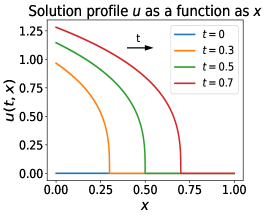
(b) medium: PME ($k(u)=u^{3}$)

(c) hard: Stefan (discont. $k(u)$)

Figure 6: Illustration of the “easy-to-hard” paradigm for PDEs, for the GPME family of conservation equations: (a) “easy” parabolic smooth (diffusion equation) solutions, with constant parameter $k(u)=k\equiv 1$; (b) “medium” degenerate parabolic PME solutions, with nonlinear monomial coefficient $k(u)=u^{m}$, with parameter $m=3$ here; and (c) “hard” hyperbolic-like (degenerate parabolic) sharp solutions (Stefan equation) with nonlinear step-function coefficient $k(u)=\bm{1}_{u\geq u^{\star}}$, where $\bm{1}_{\mathcal{E}}$ is an indicator function for event $\mathcal{E}$.

Figure 6 (Figure 1 repeated here) provides an illustration of this “easy-to-hard” paradigm for PDEs for the three classes of the GPME considered in the main text. In particular, Figure 6(a) illustrates an “easy” situation, with $k(u)\equiv 1$, where we have a simple parabolic solution to the linear heat/diffusion equation, where a sine initial condition is gradually smoothed over time. Figure 6(b) illustrates a situation with “medium” difficulty, namely the degenerate parabolic Porous Medium Equation (PME) with nonlinear differentiable monomial coefficient $k(u)=u^{m}$. Here, for $m=3$, a constant zero initial condition self-sharpens, and it develops a sharp gradient that does not dissipate over time (Maddix et al., 2018a). Finally, Figure 6(c) illustrates an example of the “hard” Stefan problem, where the coefficient $k(u)$ is a nonlinear discontinuous step-function of the unknown $u$ defined by the unknown value $u^{\star}=u(t,x^{\star}(t))=0.5$ at the discontinuity location $x^{\star}(t)$. In this case, the solution evolves as a rightward moving shock or moving interface over time (Maddix et al., 2018b).

Here, we provide more details on these and other classes of the GPME.

Heat/Diffusion Equation.

Perhaps the simplest non-trivial form of the GPME, where the conductivity or diffusivity coefficient

$$k(u)=k>0,$$

is a constant, corresponds to the heat (or diffusion) equation. In this case, Equation 9 reduces to the linear parabolic equation, $u_{t}=k\Delta u$, where $\Delta$ denotes the Laplacian operator. Solutions of this equation are smooth due to the diffusive nature of the Laplacian operator, and even sharp initial condition are smoothed over time.

Variable Coefficient Problem.

The linear variable coefficient problem

$$k(u,x)=k(x),$$

is also a classical parabolic equation. The variable coefficient problem is commonly used in reservoir simulations to model the interface between permeable and impermeable materials, where $k(u)$ denotes the step-function permeabilities that depends on the spatial position $x$.

Porous Medium Equation (PME).

Another subclass of the GPME, in which the coefficient is nonlinear but smooth, is known as the Porous Medium Equation (PME). The PME is known to be degenerate parabolic, and it becomes more challenging as $m$ increases. The PME with $m=1$ has been widely used to model isothermal processes, e.g., groundwater flow and population dynamics in biology. For $m>1$, the PME results in sharp solutions, and it has been used to describe adiabatic processes and nonlinear phenomena such as heat transfer of plasma (ionized gas).

Super-slow Diffusion Problem.

Another subclass of the GPME, known as super-slow diffusion, occurs when

$$k(u)=\exp(-1/u).$$

Here, the diffusivity $k(u)\rightarrow 0$ as $u\rightarrow 0$ faster than any power of $u$. This equation models the diffusion of solids at different absolute temperatures $u$. The coefficient $k(u)$ represents the mass diffusivity in this case, and it is connected with the Arrhenius law in thermodynamics.

Stefan Problem.

The most challenging case of the GPME is when the coefficient $k(u)$ is a discontinuous nonlinear step function:

$$k(u)=\begin{cases}k_{\max},\hskip 2.84544ptu\geq u^{\star}\\ k_{\min},\hskip 2.84544ptu<u^{\star},\end{cases}$$ (42)

for given constants $k_{\max}$, $k_{\min}$ and $u^{\star}\in\mathbb{R}$, in which case it is known as the Stefan problem. The Stefan problem has been used to model two-phase flow between water and ice, crystal growth, and more complex porous media such as foams (van der Meer et al., 2016).

We conclude by noting that, even though the GPME is nonlinear in general, for specific initial and boundary conditions, it has closed form self-similar solutions. For details, see Vázquez (2007); Maddix et al. (2018a, b). This enables ease of evaluation by comparing each competing method to the ground truth.

Appendix I Detailed Experiment Settings

In this section, we review the basics of the Attentive Neural Process (ANP) (Kim et al., 2019) that we use as the black-box deep learning model in Step 1 of our model ProbConserv-ANP in the empirical results section 3. Figure 7 illustrates a schematic for ProbConserv-ANP that shows how in the first step the mean and covariance estimates $\mu,\Sigma$ from the ANP are fed into our probabilistic constraint in the second step to output the updated mean and covariance estimates $\tilde{\mu},\tilde{\Sigma}$.

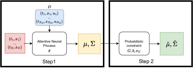
Figure 7: Schematic for the instantiation of our framework ProbConserv with the ANP (ProbConserv-ANP) as the data-driven black box model in Step 1 that is used in the empirical results. In Step 1, the ANP outputs a mean $\mu$ and covariance $\Sigma$ (yellow) of the solution profile $u$ evaluated at the $N$ target points (red). The ANP takes as input the context set $D$ that comprises $N_{D}$ labelled points (blue). The parameter $\theta$ encapsulates the neural network weights within the ANP. In Step 2, the probabilistic constraint in Equation 8 is applied yielding an updated mean $\tilde{\mu}$ and covariance $\tilde{\Sigma}$ (green). The probabilistic constraint is determined by the matrix $G$, value $b$, and variance $\sigma_{G}^{2}$ in Equation 7.

Model Training.

The model from Step 1 is data-driven, with parameter $\theta$ that needs to be learned from data. Given an empirical data distribution, written as $(u,b,D)\sim p$, we maximize the expected joint likelihood of the function $u$ and the constraint $b$, conditioned on data $D$, as a function of the Step 1 parameter $\theta$ and Step 2 parameters $\sigma_{G}$ and $G$ as follows:

$$\begin{split}L(\theta,\sigma_{G},G)&=\mathbb{E}_{u,b,D\sim p}\log p(u,b|D)\\ &=\underbrace{\mathbb{E}_{u,D\sim p}\log p_{\theta}(u|D)}_{\text{Step 1}}+\underbrace{\mathbb{E}_{u,b}\log p_{\sigma_{G},G}(b|u)}_{\text{Step 2}}.\end{split}$$ (43)

This follows because the joint probability can be broken into conditionals ${p(u,b|D)=p_{\theta}(u|D)p_{\sigma_{G},G}(b|u)}$, using Bayes’ Rule. The Step 2 constraint only depends on the value $u$.

The Step 1 parameter $\theta$ is only present in the first term of the summation in Equation 43. Then, the optimal value for $\theta^{\star}$ is found by optimizing the unconstrained log-likelihood from Step 1 over the empirical data distribution and is given as follows:

$$\begin{split}\theta^{\star}&=\operatorname*{arg\,max}_{\theta}L(\theta,\sigma_{G},G)\\ &=\operatorname*{arg\,max}_{\theta}\mathbb{E}_{u,D\sim p}\log p_{\theta}(u|D).\end{split}$$ (44)

Equation 44 is simply the optimization target of several generative models, e.g., Gaussian processes and the ANP. This justifies training the Step 1 black-box model with its original training procedure before applying our Step 2.

Data Generation.

For each PDE instance, we first generate training data for the data-driven model in Step 1. We generate these samples, indexed by $i$, by randomly sampling $n_{\text{train}}$ values of the PDE parameters $\alpha_{i}$ from an interval $\mathcal{A}$. To create the input data $D_{i}$, the solution profile corresponding to $\alpha_{i}$ is evaluated on a set of $N_{D}$ points uniformly sampled from the spatiotemporal domain $[0,t]\times\Omega$. Then, the reference solution for $u$ with parameter $\alpha_{i}$, denoted $u_{i}$, is evaluated over another set of $N_{\text{train}}$ uniformly-sampled points. The Step 1 model (ANP) is then trained on these supervised input-output pairs, $(D_{i},u_{i})$. Using Equation 5, the conservation value $b$ in Step 2 is calculated given the parameter $\alpha_{i}$. At inference time, we fix specific values of the PDE parameters $\alpha$ that are of interest and generate new input-output pairs to evaluate the predictive performance. The settings are the same as those at training, except that the reference solution is evaluated on a fixed grid that evenly divides the time domain $[0,t]$ into $T_{\text{test}}$ points and the spatial domain $\Omega$ into $M_{\text{test}}$ points for a spatio-temporal grid of $N_{\text{test}}=T_{\text{test}}\times M_{\text{test}}$ points. For consistent results, we repeat this procedure over $n_{\text{test}}$ independent datasets for each $\alpha$.

Table 6 provides the training settings and Table 7 provides the cor responding test settings.

Table 6: Training details for each instance of the GPME (Diffusion, PME, Stefan) used in the experiments.

PDE	Parameter	$\mathcal{A}$	Time domain $[0,t]$	Spatial domain $\Omega$	$n_{\text{train}}$	$N_{D}$	$N_{\text{train}}$
Diffusion	$k$	$[1,5]$	$[0,1]$	$[0,2\pi]$	10,000	$100$	$100$
PME	$m$	$[1,6]$	$[0,1]$	$[0,1]$	10,000	$100$	$100$
Stefan	$u^{\star}$	$[0.55,7]$	$[0,0.1]$	$[0,1]$	10,000	$100$	$100$

Table 7: Testing details for each instance of the GPME (Diffusion, PME, Stefan) used in the experiments.

PDE	Parameter values	Test time	Spatial domain $\Omega$	$n_{\text{test}}$	$N_{D}$	$T_{\text{test}}$	$M_{\text{test}}$	$N_{\text{test}}$
Diffusion	$k\in\{1,5\}$	$0.5$	$[0,2\pi]$	50	$100$	$201$	$201$	$40,401$
PME	$m\in\{1,3,6\}$	$0.5$	$[0,1]$	50	$100$	$201$	$201$	$40,401$
Stefan	$u^{\star}\in\{0.6\}$	$0.05$	$[0,1]$	50	$100$	$201$	$201$	$40,401$

We describe here how the input data $D$; input points $(t_{1},x_{1}),\dots,(t_{N},x_{N})$; and solution $u$ are created for a particular draw of PDE parameter $\alpha\in\mathcal{A}$. The input data (a.k.a. the context set) $D$ is generated as follows. First, draw samples from the spatiotemporal domain $(t_{n},x_{n})\sim\text{Uniform}([0,t]\times\Omega)$, for $n=1,\dots,N_{D}$. For each sample $(t_{n},x_{n})$, evaluate the reference solution $u_{n}\coloneqq u(t_{n},x_{n})$ for $\alpha$. Then $D=\{(t_{n},x_{n},u_{n})\}_{n=1,\dots,N_{D}}$.

We create input points $(t_{1},x_{1}),\dots,(t_{N},x_{N})$ differently depending on whether we are training or testing. At train-time, the input points are sampled uniformly from the spatiotemporal domain

$${(t_{n},x_{n})\sim\text{Uniform}([0,t]\times\Omega)},$$

for ${n=1,\dots,N_{\text{train}}}$. At test-time, we divide up the time domain $[0,t]$ into $T_{\text{test}}$ evenly-spaced points and the spatial domain $\Omega$ into $M_{\text{test}}$ evenly-spaced points. We then take the cross product of these as the set of input points, whose size is $N_{\text{test}}=T_{\text{test}}\times M_{\text{test}}$.

Finally, over the set of input points, we evaluate the reference solution for $\alpha$ as: $u=[u(t_{n},x_{n})]_{n=1,\dots,N_{\text{train}}}$.

Attentive Neural Processes (ANP).

The Attentive Neural Process (ANP) (Kim et al., 2019) models the conditional distribution of a function $u$ at target input points $\{x_{n}\}\coloneqq x_{1},\dots,x_{N}$ for $x_{i}\in\mathbb{R}^{D+1}$ given a small set of context points $D\coloneqq\{x_{i},u_{i}\}_{i\in C}$. The function values at each target point $x_{n}$, written as $u_{n}$, are conditionally independent given the latent variable $z$ with the following distribution for $u_{n}$:

$$\begin{split}p_{\theta}(u_{n}|D)&=\int_{z}p_{\theta}(u_{n}|z,D)p_{\theta}(z|D)dz,\\ p_{\theta}(u_{n}|z,D)&=p_{\mathcal{N}}(u_{n}|\mu_{n},\sigma^{2}_{n}),\\ p_{\theta}(z|\mu_{z},\Sigma_{z})&=p_{\mathcal{N}}(z|\mu_{z},\Sigma_{z}),\\ \mu_{n},\sigma_{n}&=f_{\theta}^{u}(x_{n},z,f_{\theta}^{r}(x_{n},D)),\\ \mu_{z},\Sigma_{z}&=f_{\theta}^{z}(D).\\ \end{split}$$ (45)

Here, $p_{\mathcal{N}}(u|\mu,\sigma^{2})\coloneqq(2\pi\sigma^{2})^{-1/2}\exp\left(-\frac{1}{2\sigma^{2}}(x-\mu)^{2}\right)$ denotes the univariate normal distribution with mean $\mu$ and variance $\sigma^{2}$ and $f_{\theta}^{z}$, $f_{\theta}^{u}$, and $f_{\theta}^{r}$ are neural networks whose architecture is described in more detail below.

As standard in variational inference, the attentive neural process (ANP) is trained to maximize the evidence lower bound (ELBO), which is a tractable lower bound to the marginal likelihood $\mathbb{E}_{u,D\sim p}\log p_{\theta}(u|D)$ that we want to maximize in Equation 44:

$$\begin{split}\mathbb{E}_{u,D\sim p}\log p_{\theta}(u|D)&\geq\mathbb{E}_{u,D\sim p}\mathbb{E}_{z\sim q_{\phi}}\log p_{\theta}(u,z|D)-\log q_{\theta}(z|u,D),\\ q_{\theta}(z|u,D)&=p_{\mathcal{N}}(z|\mu_{z}^{q},\Sigma_{z}^{q}),\\ \mu_{z}^{q},\Sigma_{z}^{q}&=f_{\theta}^{z}(D\cup\{(t_{1},x_{1},u_{1}),\dots(t_{N},x_{N},u_{N})\}).\end{split}$$ (46)

By concatenating the context set $D$ with the target set, the ANP can use the same networks for both the generative model $p_{\theta}$ and the variational model $q_{\theta}$. This differs from methods such as the variational auto-encoder (VAE) that train a separate network for the variational model.

In the experiments, we train the ELBO in Equation 46 using stochastic gradient descent over random mini-batches of the supervised pairs $(u,D)$ and a sample of the latent variable $z$ (using the reparameterization trick for an unbiased gradient estimate). Specifically, we use the ADAM optimizer with a learning rate of $1\times 10^{-4}$ and a batch size of $250$.

Architectural details.

Here, we briefly describe the architecture of the ANP used in experiments; a more thorough description of the ANP in general can be found in the original paper (Kim et al., 2019).

The ANP consists of three distinct networks:

1. The latent encoder $f_{\theta}^{z}$ takes the context set $D=\{x_{i},u_{i}\}_{i\in C}$ as input and outputs a mean $\mu_{z}$ and diagonal covariance $\Sigma_{z}$ for the latent representation $z$. Note that $f_{\theta}^{z}$ is invariant to the order of the context set inputs in $D$.

2. The deterministic encoder $f_{\theta}^{r}$ takes the context set $D=\{x_{i},u_{i}\}_{i\in C}$ and the target points $\{x_{n}\}$ as input, and outputs a set of deterministic representations $\{r_{n}\}$ corresponding to each target point. Note that $f_{\theta}^{r}$ is permutation-invariant to the order of the context set inputs in $D$, and is applied pointwise across the target inputs $\{x_{n}\}$.

3. The decoder $f_{\theta}^{u}$ takes the outputs from the latent encoder, deterministic encoder, and the target points $\{x_{n}\}$ as input, and outputs a set of mean and variances $\{\mu_{n},\sigma_{n}\}$ corresponding to each target point. The decoder is applied pointwise across the target inputs $\{x_{n}\}$ and deterministic representation $\{r_{n}\}$.

Table 8: ANP hyperparameters.

Symbol	Value	Description
$d_{x}$	2	Input dimension
$d_{u}$	1	Output dimension
$d_{z}$	128	Latent dimension
$h$	128	Size of hidden layer
$n_{\text{heads}}$	4	Number of heads in MultiHead
$d_{h}$	128	Column dimension in MultiHead layers

For reproducibility, Figure 8 shows how each network is constructed and Table 8 shows the ANP hyperparameters. Each building blocks is also briefly described below:

• $\text{Linear}(d_{\text{in}},d_{\text{out}})$: dense linear layer $xA+b$.

• Mean: Averages the inputs of the input set; i.e., $\text{Mean}(\{s_{i}\})=\frac{1}{|\{s_{i}\}|}\sum_{i}s_{i}$.

• ReLU: Applies ReLU activation pointwise.

• Cross-Attention and Self-Attention. These are multi-head attention blocks first introduced in Vaswani et al. (2017). The three inputs to the multi-head attention block are the queries $Q=[q_{1}|\dots|q_{d_{q}}]^{\top}$, keys $K=[k_{1}|\dots|q_{d_{k}}]^{\top}$, and values $V=[v_{1}|\dots|v_{d_{k}}]^{\top}$. The hyperparameters are the number of heads, $n_{\text{heads}}$ and the number of columns of the matrices $W_{i}^{Q},W_{i}^{K},W_{i}^{V}$, denoted as $d_{h}$. We summarize the notations below:

  $$\begin{split}\text{Self-Attention}(Q)&\coloneqq\text{MultiHead}(Q,Q,Q),\\ \text{Cross-Attention}(Q,K,V),&\coloneqq\text{MultiHead}(Q,K,V),\\ \text{MultiHead}(Q,K,V)&\coloneqq[H_{1}|\dots|H_{n_{\text{heads}}}]W^{O},\\ H_{i}&\coloneqq\text{Attention}(QW_{i}^{Q},KW_{i}^{K},VW_{i}^{V}),\\ \mathrm{Attention}(Q,K,V)&\coloneqq\mathrm{softmax}\left(\frac{QK^{\top}}{\sqrt{d_{k}}}\right)V,\\ \mathrm{softmax}\left(\begin{bmatrix}x_{1,1}&\dots&x_{1,n}\\ \vdots&\ddots&\vdots\\ x_{m,1}&\dots&x_{m,n}\end{bmatrix}\right)&\coloneqq\begin{bmatrix}\frac{\exp(x_{1,1})}{\sum_{i=j}^{n}\exp(x_{1,j})}&\dots&\frac{\exp(x_{1,n})}{\sum_{j=1}^{n}\exp(x_{1,j})}\\ \vdots&\ddots&\vdots\\ \frac{\exp(x_{m,1})}{\sum_{i=1}^{m}\exp(x_{m,j})}&\dots&\frac{\exp(x_{m,n})}{\sum_{j=1}^{n}\exp(x_{m,j})}\end{bmatrix}.\\ \end{split}$$

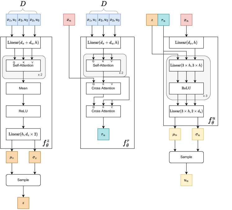
Figure 8: Architectural diagram of the three main networks that make up the Attentive Neural Process (ANP) from Kim et al. (2019) that is used in the experiments as the Step 1 black-box model.

Appendix J Additional Empirical Results

In this section, we provide additional empirical results for the degenerate parabolic Generalized Porous Medium (GPME) family of conservation laws as well as for hyperbolic conservation laws.

J.1 GPME Family of Conservation Laws

Here, we include additional solution profiles and conservation profiles over time for the GPME family of equations, ranging from the “easy" diffusion (heat), “medium" PME, to the “hard" Stefan equations.

J.1.1 Diffusion (Heat) Equation

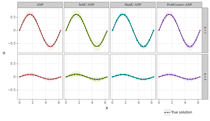
Figure 9: Solution profiles for the diffusion (heat) equation at time $t=0.5$ for diffusivity (conductivity) test-time parameter $k=1$ in the top row and $k=5$ in the bottom row. Each model is trained on samples of $k\in\mathcal{A}=[1,5]$. The shaded region illustrates $\pm 3$ standard deviation uncertainty intervals. ProbConserv-ANP and HardC-ANP both display tighter uncertainty bounds than the baseline ANP, while SoftC-ANP is more diffuse. The uncertainty is relatively homoscedastic on this “easy” case.

Solution Profiles.

Figure 9 shows the solution profiles for the “easy" diffusion equation, at time $t=0.5$, where a sine curve is damped over time for test-time parameter $k=1,5\in\mathcal{A}=[1,5]$. Table 9 shows the corresponding metrics.

Table 9: Mean and standard error for CE $\times 10^{-3}$ (should be zero), LL (higher is better) and MSE $\times 10^{-4}$ (lower is better) over $n_{\text{test}}=50$ for the (“easy") diffusion equation at time $t=0.5$ with variable diffusivity constant $k$ parameter in the range $\mathcal{A}=[1,5]$ and test-time parameter values $k=1,5$.

	$k=1$			$k=5$
	CE	LL	MSE	CE	LL	MSE
ANP	4.68 (0.10)	$2.72$ (0.02)	$1.71$ (0.41)	1.76 (0.04)	$3.28$ (0.02)	$0.547$ (0.08)
SoftC-ANP	3.47 (0.17)	$2.40$ (0.02)	$2.24$ (0.78)	2.86 (0.05)	$2.83$ (0.02)	$1.75$ (0.24)
HardC-ANP	0 (0.00)	3.08 (0.04)	$\mathbf{1.37}$ (0.33)	0 (0.00)	3.64 (0.03)	$\mathbf{0.461}$ (0.07)
ProbConserv-ANP	0 (0.00)	2.74 (0.02)	1.55 (0.33)	0 (0.00)	3.30 (0.02)	0.485 (0.07)

J.1.2 Porous Medium Equation (PME)

Results for Different $\lambda$ for SoftC-ANP.

As is the case with PINNs (Raissi et al., 2019), the SoftC-ANP method has a hyper-parameter $\lambda$ that controls the balance in the training loss between the reconstruction and differential term. A higher value of $\lambda$ places more emphasis on the residual of the PDE term and less emphasis on the evidence lower bound (ELBO) from the ANP.

To investigate whether tuning $\lambda$ will lead to significantly different results, we report results for different values of $\lambda$ for the SoftC-ANP on the Porous Medium Equation (PME). Since these results are presented on the same test dataset used in Table 2, it provides an optimistic case on how tuning $\lambda$ could improve the results for SoftC-ANP. Table 10 shows that the predictive performance is roughly the same across different values of $\lambda$, with both MSE and LL worse than the original ANP across the board and the conservation error (CE) $G\mu-b$ at the final time worse for $m=6$.

Table 10: Investigation of the effect of the soft constraint penalty parameter $\lambda$ in the SoftC-ANP baseline. The metrics CE $\times 10^{-3}$ (should be zero), LL (higher is better) and MSE $\times 10^{-4}$ (lower is better) are reported for the (“medium") PME at time $t=0.5$ with variable $m$ parameter in the range $\mathcal{A}=[0.99,6]$ and test-time parameters $m\in\{1,3,6\}$. We see that the performance is not significantly changed as a function of $\lambda$, and, surprisingly, that the unconstrained ANP ($\lambda=0)$ performs better in most metrics than SoftC-ANP.

	$m=1$			$m=3$			$m=6$
	CE	LL	MSE	CE	LL	MSE	CE	LL	MSE
ANP $(\lambda=0)$	$6.67$	$\bf{3.49}$	$\bf{0.94}$	$-1.23$	$\bf{3.67}$	$\bf{1.90}$	$\bf{-2.58}$	$\bf{3.81}$	$\bf{7.62}$
SoftC-ANP $(\lambda=0.01)$	$5.58$	$3.11$	$1.11$	$-0.61$	$3.46$	$2.03$	$-3.00$	$3.49$	$7.76$
SoftC-ANP $(\lambda=0.1)$	$5.58$	$3.11$	$1.11$	$-0.67$	$3.46$	$2.07$	$-3.01$	$3.49$	$7.87$
SoftC-ANP $(\lambda=1)$	$5.62$	$3.11$	$1.11$	$-0.65$	$3.46$	$2.06$	$-3.03$	$3.49$	$7.82$
SoftC-ANP $(\lambda=10)$	$\bf{5.52}$	$3.11$	$1.08$	$\bf{-0.56}$	$3.46$	$2.04$	$-3.02$	$3.49$	$7.76$
SoftC-ANP $(\lambda=100)$	$5.62$	$3.11$	$1.11$	$-0.59$	$3.46$	$2.03$	$-3.03$	$3.49$	$7.69$

ProbConserv-ANP with Diffusion.

As described in subsection D.2, we explore adding numerical diffusion for eliminating artificial small-scale noises when enforcing conservation. Table 11 shows that adding artificial diffusion improves both MSE and LL compared to the conservation constraint alone. Figures 10-11 illustrate that by removing such artificial noises, ProbConserv-ANP with diffusion leads to tighter uncertainty bounds as well as higher LL than the other baselines.

Table 11: Mean and standard error for CE $\times 10^{-3}$ (should be zero), LL (higher is better) and MSE $\times 10^{-4}$ (lower is better) over $n_{\text{test}}=50$ runs for the (“medium”) PME at time $t=0.5$ with variable $m$ parameter in the range $\mathcal{A}=[0.99,6]$. We see that ProbConserv-ANP (w/diff) improves the performance on ProbConserv-ANP by applying smoothing at the sharp boundary as the test-time parameter $m$ is increased.

	$m=1$			$m=3$			$m=6$
	CE	LL	MSE	CE	LL	MSE	CE	LL	MSE
ANP	$6.67$ (0.39)	$3.49$ (0.01)	$0.94$ (0.09)	$-1.23$ (0.29)	$3.67$ (0.00)	$1.90$ (0.04)	$-2.58$ (0.23)	$3.81$ (0.01)	7.67 (0.09)
SoftC-ANP	$5.62$ (0.35)	$3.11$ (0.01)	$1.11$ (0.14)	$-0.65$ (0.30)	$3.46$ (0.00)	$2.06$ (0.03)	$-3.03$ (0.26)	$3.49$ (0.00)	$7.82$ (0.09)
HardC-ANP	0 (0.00)	3.16 (0.04)	0.43 (0.04)	0 (0.00)	$3.44$ (0.03)	1.86 (0.03)	0 (0.00)	3.40 (0.05)	7.61 (0.09)
ProbConserv-ANP	0 (0.00)	3.56 (0.01)	0.17 (0.02)	0 (0.00)	3.68 (0.00)	2.10 (0.07)	0 (0.00)	3.83 (0.01)	10.4 (0.04)
ProbConserv-ANP (w/diff)	0 (0.00)	4.04 (0.02)	0.15 (0.02)	0 (0.00)	3.96 (0.00)	1.43 (0.05)	0 (0.00)	4.03 (0.01)	7.91 (0.03)

Solution and Error Profiles.

Figures 10-11 illustrate the differing solution profiles and errors for the PME for various values of $m\in\{1,3,6\}$, respectively. As expected, we see a gradient for $m>1$ that becomes sharper and approaches infinity for $m=6$. Increasing $m$ results in smaller values of the PDE parameter denoting the pressure $k(u)=u^{m}$, which increases the degeneracy for smaller values of $k(u)$, i.e., larger values of $m$. In this case the problem also becomes more challenging. For $m=1$, we have a piecewise linear solution, and for $m=3,6$ we see sharper oscillatory uncertainty bounds at the front or free boundary, resulting in some negative values at this boundary as well. We see the value of the uncertainty quantification to reflect that the model is certain in the parabolic regions to the left and right of the sharp boundary especially in the zero (degeneracy) region, and is most uncertain at the boundary (degeneracy) point.

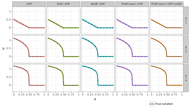
Figure 10: Solution profiles and uncertainty intervals for the PME predicted by our ProbConserv-ANP and other baselines. The solutions are obtained for three scenarios with increasing sharpness in the profile as $m$ is increased from $m=1$ to $m=6$ from left to right, respectively. The HardC-ANP model, which assumes constant variance for the whole domain, results in too high uncertainty in the zero (degenerate) region, unlike our proposed ProbConserv-ANP approach that incorporates the variance information to effectively handle this heteroscedasticity. Adding diffusion to ProbConserv-ANP removes the oscillations locally at the degeneracy, as desired.

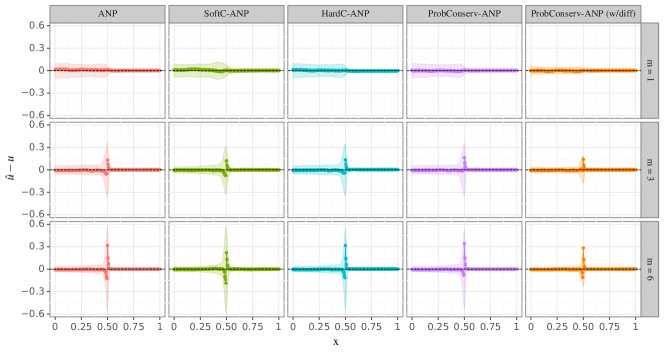
Figure 11: Solution errors with uncertainty bounds as a function of $x$ for our ProbConserv-ANP and other baselines for the PME with parameter $m\in\{1,3,6\}$ after training on $m\in\mathcal{A}=[0.99,6]$. The shaded region indicates $\pm 3$ standard deviations as estimated by each model. For $m=1$, both ProbConserv-ANP with and without diffusion result in solutions with smaller errors. While HardC-ANP model reduces the error scale, it underestimates the zero portion of the solution, which is nonphysical, as the solution quantity cannot be negative. For $m\in\{3,6\}$, while the error magnitude becomes dominant at the shock position for all methods, ProbConserv-ANP with diffusion provides the lowest errors with the tightest confidence interval.

J.1.3 Stefan

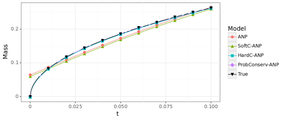
Figure 12: True mass over time for each model. The true mass conservation profile over time is matched exactly by our proposed method ProbConserv-ANP and the hard-constrained HardC-ANP by design. The unconstrained ANP and surprisingly even the differential form soft-constrained SoftC-ANP have a non-physical linear mass profile over time.

Figure 12 shows ProbConserv-ANP follows the true profile of conserved mass in the system over time by design. We also see that the unconstrained ANP and surprisingly the soft-constrained SoftC-ANP that applied the differential form as a soft constraint does not result in conservation being satisfied since it does not enforce it exactly. For these baselines, the mass profile over time is linear and does not match the true profile which is proportional to $\sqrt{t}$.

J.2 Hyperbolic Equations

Here, we demonstrate that our approach ProbConserv-ANP also works for hyperbolic conservation laws by considering the linear advection problem (“medium”) and Burgers’ equation (“hard”), which are both introduced in Table 5 in Appendix C.

J.2.1 Linear Advection

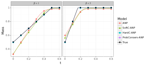
Figure 13: System total mass as a function of time $t$ for the linear advection problem with test-time parameter $\beta=1,3$ and training parameter range $\mathcal{A}=[1,5]$. Both ProbConserv-ANP and HardC-ANP satisfy conservation of mass while the unconstrained ANP and soft-constrained SoftC-ANP baselines deviate from the actual trend completely at all times.

Figure 13 displays the system total mass, $U(t)=\int_{\Omega}u(t,x)d\Omega$ as a function of time, obtained by our ProbConserv-ANP model and the other baselines and compared against the true curve. The results are obtained for two values of test-time parameter $\beta=1,3$ denoting the velocity with training range $\beta\in\mathcal{A}=[1,5]$. The unconstrained ANP contradicts the system true mass at all times including $t=0$. By proper incorporation of the conservation constraint, both ProbConserv-ANP and HardC-ANP methods are able to predict the system mass and capture the actual trend over time exactly while the soft-constrained differential form SoftC-ANP baseline results in little improvement.

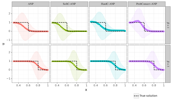
Figure 14: Solution profiles and uncertainty intervals for linear advection problem at time $t=0.1$ for test-time parameter $\beta=1,3$ and training parameter range $\mathcal{A}=[1,5]$. Despite satisfaction of conservation constraint, HardC-ANP predicts a highly diffusive profile and remarkable underestimation of shock interface region especially for $\beta=1$. The prediction error is even higher for the unconstrained ANP model which does not enforce the conservation, and the shock interface is shifted further away from the true solution. ProbConserv-ANP results in a sharper profile than other the baselines and the predicted shock interface is around the actual shock position leading to more accurate shock position estimation.

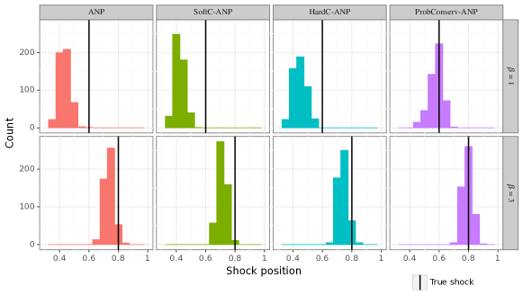
Figure 15: The histogram of shock position for the linear advection problem, computed as the mean plus or minus 3 standard deviations. Due to the shift in the shock interface, both the ANP and HardC-ANP models underestimate the position of the shock, and the underestimation is more significant for $\beta=1$. The ProbConserv-ANP model provides a histogram distributed almost symmetrically around the true shock interface and thus leads to an accurate estimate of the shock position.

Figure 14 shows the predicted solution profiles and corresponding uncertainty intervals for time $t=0.1$ and test-time parameter $\beta=1,3$. Our ProbConserv-ANP model predicts sharper shock profile centered around the actual shock position. On the contrary, both ANP and HardC-ANP lead to highly diffusive profiles which are shifted toward the left of actual shock interface, leading to the under-estimation of the shock position on this downstream task. This under-estimation becomes more evident in Figure 15, which indicates the corresponding histograms of shock position. The histograms associated with the ANP and HardC-ANP models are skewed to the left and both result in the averaged shock positions which are lower than the actual value depicted by the solid vertical line. By proper leveraging of our finite volume based physical constraint, our ProbConserv-ANP results in proper uncertainty quantification which leads to accurate prediction of shock location compared to the other baseline models. Table 12 also shows this accuracy improvement with a maximum improvement of $2.86\times$ in MSE for $\beta=1$.

Table 12: Mean and standard error for CE (should be zero), LL (higher is better) and MSE $\times 10^{-2}$ (lower is better) over $n_{\text{test}}=50$ runs for the hyperbolic linear advection problem at time $t=0.1$ with variable $\beta$ parameter in the range $\mathcal{A}=[1,5]$.

	$\beta=1$			$\beta=3$
	CE	LL	MSE	CE	LL	MSE
ANP	-0.136 (0.004)	0.96 (0.01)	5.72 (0.25)	0.042 (0.003)	0.51 (0.01)	2.03 (0.01)
SoftC-ANP	-0.137 (0.004)	1.58 (0.03)	7.64 (0.34)	0.013 (0.003)	2.31 (0.02)	2.87 (0.20)
HardC-ANP	0 (0.00)	-2.96 (0.34)	4.59 (0.17)	0 (0.00)	1.34 (0.21)	1.93 (0.07)
ProbConserv-ANP	0 (0.00)	1.06 (0.01)	2.00 (0.06)	0 (0.00)	0.52 (0.01)	1.62 (0.01)

J.2.2 Burgers’ Equation

Figure 16 illustrates that the total mass is linear over time, and in this case is approximately satisfied by our ProbConserv-ANP and the baselines. Figure 17 shows the waiting time phenomenon, where the piecewise linear initial condition self-sharpens until the breaking time $t_{b}=1/a$, where it forms a rightward moving shock. We see that the breaking time is inversely proportional to the slope, and that the shock forms sooner for larger values of $a$.

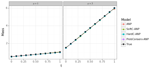
Figure 16: True mass as a function of time $t$ for the Burgers’ equation with test-time parameter $a=1,3$ and training parameter range $\mathcal{A}=[1,4]$.

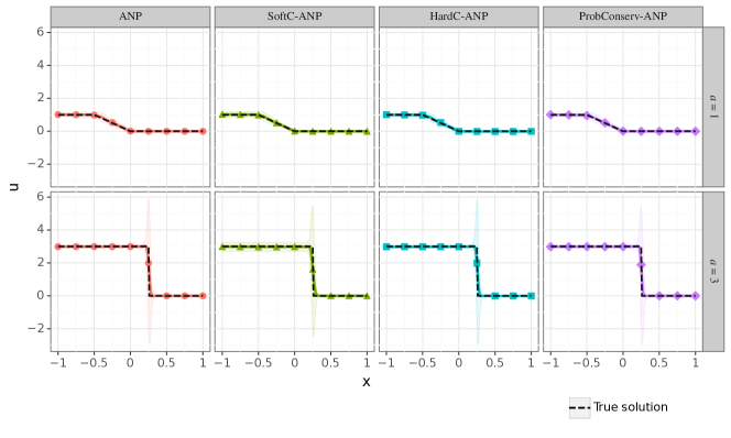
Figure 17: Solution profiles and uncertainty intervals for Burgers’ equation at time $t=0.5$ for test-time parameter $a=1,3$ and training parameter range $\mathcal{A}=[1,4]$.

References

- Al-Rawahi & Tryggvason (2002) Al-Rawahi, N. and Tryggvason, G. Numerical simulation of dendritic solidification with convection: Two-dimensional geometry. Journal of Computational Physics, 180(2):471–496, 2002.
- Beucler et al. (2021) Beucler, T., Pritchard, M., Rasp, S., Ott, J., Baldi, P., and Gentine, P. Enforcing Analytic Constraints in Neural-Networks Emulating Physical Systems. Physical Review Letters, 126(9):098302, 2021.
- Bolton & Zanna (2019) Bolton, T. and Zanna, L. Applications of Deep Learning to Ocean Data Inference and Subgrid Parameterization. Journal of Advances in Modeling Earth Systems, 11(1):376–399, 2019.
- Burden et al. (2016) Burden, A., Burden, R., and Faires, J. Numerical Analysis. CENGAGE Learning, 10th edition, 2016.
- Chen et al. (2018) Chen, R. T. Q., Rubanova, Y., Bettencourt, J., and Duvenaud, D. K. Neural ordinary differential equations. In Advances in Neural Information Processing Systems, volume 31, 2018.
- Chen et al. (1997) Chen, S., Merriman, B., Osher, S., and Smereka, P. A simple level set method for solving stefan problems. Journal of Computational Physics, 135(1):8–29, 1997.
- Edwards (2022) Edwards, C. Neural networks learn to speed up simulations. Communications of the ACM, 65(5):27–29, 2022.
- Evans (2010) Evans, L. Partial Differential Equations, volume 19 of Graduate studies in mathematics. American Mathematical Society, 2nd edition, 2010.
- Gelman et al. (2015) Gelman, A., Carlin, J. B., Stern, H. S., Dunson, D. B., Vehtari, A., and Rubin, D. B. Bayesian Data Analysis. Chapman and Hall/CRC, New York, third edition, July 2015.
- Goswami et al. (2022) Goswami, S., Bora, A., Yu, Y., and Karniadakis, G. E. Physics-informed deep neural operator networks. arXiv preprint arXiv:2207.05748, 2022.
- Gupta et al. (2021) Gupta, G., Xiao, X., and Bogdan, P. Multiwavelet-based Operator Learning for Differential Equations. In Advances in Neural Information Processing Systems, volume 34, 2021.
- Hastie et al. (2013) Hastie, T., Tibshirani, R., and Friedman, J. The Elements of Statistical Learning: Data Mining, Inference, and Prediction. Springer Series in Statistics. Springer New York, 2013.
- Jacot et al. (2018) Jacot, A., Gabriel, F., and Hongler, C. Neural tangent kernel: Convergence and generalization in neural networks. In Advances in Neural Information Processing Systems, volume 31, 2018.
- Jagtap et al. (2020) Jagtap, A. D., Kharazmi, E., and Karniadakis, G. E. Conservative physics-informed neural networks on discrete domains for conservation laws: Applications to forward and inverse problems. Computer Methods in Applied Mechanics and Engineering, 365:113028, 2020.
- Jekel et al. (2022) Jekel, C. F., Sterbentz, D. M., Aubry, S., Choi, Y., White, D. A., and Belof, J. L. Using conservation laws to infer deep learning model accuracy of Richtmyer-meshkov instabilities. arXiv preprint arXiv:2208.11477, 2022.
- Kim et al. (2019) Kim, H., Mnih, A., Schwarz, J., Garnelo, M., Eslami, A., Rosenbaum, D., Vinyals, O., and Teh, Y. W. Attentive Neural Processes. arXiv preprint arXiv:1901.05761, 2019.
- Krishnapriyan et al. (2021) Krishnapriyan, A. S., Gholami, A., Zhe, S., Kirby, R., and Mahoney, M. W. Characterizing possible failure modes in physics-informed neural networks. In Advances in Neural Information Processing Systems, volume 34, pp. 26548–26560, 2021.
- Krishnapriyan et al. (2022) Krishnapriyan, A. S., Queiruga, A. F., Erichson, N. B., and Mahoney, M. W. Learning continuous models for continuous physics. arXiv preprint arXiv:2202.08494, 2022.
- LeVeque (1990) LeVeque, R. J. Numerical Methods for Conservation Laws. Lectures in mathematics ETH Zürich. Birkhäuser Verlag, 1990.
- LeVeque (2002) LeVeque, R. J. Finite Volume Methods for Hyperbolic Problems. Cambridge University Press, 2002.
- LeVeque (2007) LeVeque, R. J. Finite Difference Methods for Ordinary and Partial Differential Equations: Steady-State and Time-Dependent Problems. SIAM, 2007.
- Li et al. (2003) Li, C.-Y., Garimella, S. V., and Simpson, J. E. Fixed-grid front-tracking algorithm for solidification problems, Part I: Method and validation. Numerical Heat Transfer, Part B: Fundamentals, 43(2):117–141, 2003.
- Li et al. (2020) Li, Z., Kovachki, N., Azizzadenesheli, K., Liu, B., Bhattacharya, K., Stuart, A., and Anandkumar, A. Neural Operator: Graph Kernel Network for Partial Differential Equations. arXiv preprint arXiv:2003.03485, 2020.
- Li et al. (2021a) Li, Z., Kovachki, N., Azizzadenesheli, K., Liu, B., Bhattacharya, K., Stuart, A., and Anandkumar, A. Fourier Neural Operator for Parametric Partial Differential Equations. In International Conference on Learning Representations, 2021a.
- Li et al. (2021b) Li, Z., Zheng, H., Kovachki, N. B., Jin, D., Chen, H., Liu, B., Azizzadenesheli, K., and Anandkumar, A. Physics-informed neural operator for learning partial differential equations. arXiv preprint arXiv:2111.03794, 2021b.
- Lipnikov et al. (2016) Lipnikov, K., Manzini, G., Moulton, J. D., and Shashkov, M. The mimetic finite difference method for elliptic and parabolic problems with a staggered discretization of diffusion coefficient. Journal of Computational Physics, 305:111–126, 2016.
- Lu et al. (2021) Lu, L., Jin, P., Pang, G., Zhang, Z., and Karniadakis, G. E. Learning nonlinear operators via deeponet based on the universal approximation theorem of operators. Nat. Mach. Intell., 3:218–229, 2021.
- Maddix et al. (2018a) Maddix, D. C., Sampaio, L., and Gerritsen, M. Numerical artifacts in the Generalized Porous Medium Equation: Why harmonic averaging itself is not to blame. Journal of Computational Physics, 361:280–298, 2018a.
- Maddix et al. (2018b) Maddix, D. C., Sampaio, L., and Gerritsen, M. Numerical artifacts in the discontinuous Generalized Porous Medium Equation: How to avoid spurious temporal oscillations. Journal of Computational Physics, 368:277–298, 2018b.
- Mao et al. (2020) Mao, Z., Jagtap, A. D., and Karniadakis, G. E. Physics-informed neural networks for high-speed flows. Computer Methods in Applied Mechanics and Engineering, 360:112789, 2020.
- Müller (2022) Müller, E. H. Exact conservation laws for neural network integrators of dynamical systems. arXiv preprint arXiv:2209.11661, 2022.
- Négiar et al. (2023) Négiar, G., Mahoney, M. W., and Krishnapriyan, A. S. Learning differentiable solvers for systems with hard constraints. In International Conference on Learning Representations, 2023.
- Onken & Ruthotto (2020) Onken, D. and Ruthotto, L. Discretize-optimize vs. optimize-discretize for time-series regression and continuous normalizing flows. arXiv preprint arXiv:2005.13420, 2020.
- Osher & Sethian (1988) Osher, S. and Sethian, J. A. Fronts propagating with curvature-dependent speed: Algorithms based on hamilton-jacobi formulations. Journal of Computational Physics, 79:12–49, 1988.
- Ott et al. (2021) Ott, K., Katiyar, P., Hennig, P., and Tiemann, M. ResNet after all: Neural ODEs and their numerical solution. In International Conference on Learning Representations, 2021.
- Petersen et al. (2008) Petersen, K. B., Pedersen, M. S., et al. The matrix cookbook. Technical University of Denmark, 7(15):510, 2008.
- Raissi et al. (2019) Raissi, M., Perdikaris, P., and Karniadakis, G. Physics-informed neural networks: A deep learning framework for solving forward and inverse problems involving nonlinear partial differential equations. Journal of Computational Physics, 378:686–707, 2019.
- Rasmussen & Williams (2006) Rasmussen, C. and Williams, C. Gaussian Processes for Machine Learning. MIT Press, 2006.
- Richter-Powell et al. (2022) Richter-Powell, J., Lipman, Y., and Chen, R. T. Q. Neural conservation laws: A divergence-free perspective. arXiv preprint arXiv:2210.01741, 2022.
- Saad et al. (2023) Saad, N., Gupta, G., Alizadeh, S., and Maddix, D. Guiding continuous operator learning through physics-based boundary constraints. In International Conference on Learning Representations, 2023.
- Sargsyan (2016) Sargsyan, S. Dimensionality hyper-reduction and machine learning for dynamical systems with varying parameters. In Ph.D. Thesis, University of Washington, 2016.
- Sethian & Strain (1992) Sethian, J. A. and Strain, J. Crystal growth and dendritic solidification. Journal of Computational Physics, 98(2):231–253, 1992.
- Sturm & Wexler (2022) Sturm, P. O. and Wexler, A. S. Conservation laws in a neural network architecture: enforcing the atom balance of a julia-based photochemical model (v0.2.0). Geosci. Model Dev., 15:3417–3431, 2022.
- Subramanian et al. (2022) Subramanian, S., Kirby, R. M., Mahoney, M. W., and Gholami, A. Adaptive self-supervision algorithms for physics-informed neural networks. arXiv preprint arXiv:2207.04084, 2022.
- Tezaur et al. (2017) Tezaur, I. K., Fike, J. A., Carlberg, K. T., Barone, M. F., Maddix, D., Mussoni, E. E., and Balajewicz, M. Advanced fluid reduced order models for compressible flow. Sandia National Laboratories Report, Sand No. 2017-10335, 2017.
- van der Meer et al. (2016) van der Meer, J., Kraaijevanger, J., Möller, M., and Jansen, J. Temporal oscillations in the simulation of foam enhanced oil recovery. ECMOR XV - 15th European Conference on the Mathematics of Oil Recovery, pp. 1–20, 2016.
- Vaswani et al. (2017) Vaswani, A., Shazeer, N., Parmar, N., Uszkoreit, J., Jones, L., Gomez, A. N., Kaiser, Ł., and Polosukhin, I. Attention is all you need. In Advances in Neural Information Processing Systems, volume 30, 2017.
- Vázquez (2007) Vázquez, J. The Porous Medium Equation: Mathematical Theory. The Clarendon Press, Oxford University Press, Oxford, 2007.
- Wang et al. (2022) Wang, S., Yu, X., and Perdikaris, P. When and why pinns fail to train: A neural tangent kernel perspective. Journal of Computational Physics, 449(110768), 2022.
- Zanna & Bolton (2020) Zanna, L. and Bolton, T. Data-Driven Equation Discovery of Ocean Mesoscale Closures. Geophysical Research Letters, 47(17), 2020.