A convergent finite-volume scheme for
nonlocal cross-diffusion systems
for multi-species populations

Abstract.

An implicit Euler finite-volume scheme for a nonlocal cross-diffusion system on the one-dimensional torus, arising in population dynamics, is proposed and analyzed. The kernels are assumed to be in detailed balance and satisfy a weak cross-diffusion condition. The latter condition allows for negative off-diagonal coefficients and for kernels defined by an indicator function. The scheme preserves the nonnegativity of the densities, conservation of mass, and production of the Boltzmann and Rao entropies. The key idea is to “translate” the entropy calculations for the continuous equations to the finite-volume scheme, in particular to design discretizations of the mobilities, which guarantee a discrete chain rule even in the presence of nonlocal terms. Based on this idea, the existence of finite-volume solutions and the convergence of the scheme are proven. As a by-product, we deduce the existence of weak solutions to the continuous cross-diffusion system. Finally, we present some numerical experiments illustrating the behavior of the solutions to the nonlocal and associated local models.

1. Introduction

This paper is devoted to the design and analysis of structure-preserving finite-volume discretizations of the following one-dimensional nonlocal cross-diffusion initial-value problem:

(1) $$\partial_{t}u_{i}=\partial_{x}(\sigma\partial_{x}u_{i}+u_{i}\partial_{x}p_{i}(u))\quad\mbox{in }{\mathbb{T}},\ t>0,$$

(2) $$u_{i}(\cdot,0)=u_{i}^{0}\quad\mbox{in }{\mathbb{T}},\ i=1,\ldots,n,$$

where $\sigma\geq 0$ is the diffusion coefficient, ${\mathbb{T}}:={\mathbb{R}}/{\mathbb{Z}}$ is the one-dimensional torus of unit measure, and $p_{i}$ is the nonlocal operator

(3) $$p_{i}(u)(x):=a_{ii}u_{i}(x)+\sum_{\begin{subarray}{c}j=1\\ j\neq i\end{subarray}}^{n}a_{ij}(B^{ij}*u_{j})(x)=a_{ii}u_{i}(x)+\sum_{\begin{subarray}{c}j=1\\ j\neq i\end{subarray}}^{n}\int_{\mathbb{T}}a_{ij}B^{ij}(x-y)u_{j}(y)dy,$$

where $a_{ij}$ are some constants. The kernel functions $B^{ij}:{\mathbb{T}}\to{\mathbb{R}}$ are periodically extended to ${\mathbb{R}}$, and $u=(u_{1},\ldots,u_{n})$ is the solution vector. If we define $B^{ii}=\delta_{0}$, where $i\in\{1,\ldots,n\}$ and $\delta_{0}$ is the Dirac measure, we can rewrite $p_{i}$ as

(4) $$p_{i}(u)=\sum_{j=1}^{n}a_{ij}(B^{ij}*u_{j})(x).$$

Equations (1) with definition (4) and general kernels $B^{ij}$ for $i,j=1,\ldots,n$ can be derived from stochastic interacting particle systems in the many-particle limit [10].

We proved in [16] that the “full” nonlocal system, i.e. system (1) and (4), where $B^{ii}\neq\delta_{0}$ are general kernels, admits global weak solutions. Our analysis was based on the fact that this system possesses two Lyapunov functionals. More precisely, assume that there exist numbers $\pi_{1},\ldots,\pi_{n}>0$ such that the kernels $B^{ij}$ satisfy the so-called detailed-balance condition

$$\pi_{i}a_{ij}B^{ij}(x-y)=\pi_{j}a_{ji}B^{ji}(y-x)\quad\mbox{for }i,j=1,\ldots,n\mbox{ and a.e. }x,y\in{\mathbb{T}},$$

and the positive semi-definiteness condition

(5) $$\sum_{i,j=1}^{n}\int_{\mathbb{T}}\int_{{\mathbb{T}}}\pi_{i}a_{ij}B^{ij}(x-y)v_{j}(y)v_{i}(x)dydx\geq 0\quad\mbox{for all }v_{i},v_{j}\in L^{2}({\mathbb{T}}).$$

Then we proved that the Boltzmann (type) and Rao (type) entropies, respectively,

$$H_{B}(u) =\sum_{i=1}^{n}\int_{\mathbb{T}}\pi_{i}u_{i}(\log u_{i}-1)dx,$$

$$H_{R}(u) =\frac{1}{2}\sum_{i,j=1}^{n}\int_{\mathbb{T}}\int_{{\mathbb{T}}}\pi_{i}a_{ij}B^{ij}(x-y)u_{j}(y)u_{i}(x)\,dydx,$$

fulfill the following entropy dissipation inequalities:

(6) $$\frac{dH_{B}}{dt}+4\sigma\sum_{i=1}^{n}\int_{\mathbb{T}}\pi_{i}|\partial_{x}\sqrt{u_{i}}|^{2}dx \leq-\sum_{i,j=1}^{n}\int_{\mathbb{T}}\int_{{\mathbb{T}}}\pi_{i}a_{ij}B^{ij}(x-y)\partial_{x}u_{j}(y)\partial_{x}u_{i}(x)dydx,$$

(7) $$\frac{dH_{R}}{dt}+\sum_{i=1}^{n}\int_{\mathbb{T}}\pi_{i}u_{i}|\partial_{x}p_{i}(u)|^{2}dx \leq-\sigma\sum_{i,j=1}^{n}\int_{\mathbb{T}}\int_{{\mathbb{T}}}\pi_{i}a_{ij}B^{ij}(x-y)\partial_{x}u_{j}(y)\partial_{x}u_{i}(x)dydx,$$

and the right-hand sides are nonpositive due to (5). The Boltzmann entropy is related to the thermodynamic entropy of the system, and the Rao entropy is a measure of the functional diversity of the species [21].

While this theoretical framework was suitable to prove the existence of weak solutions, condition (5) is cumbersome to check in practice. In [16, Remark 1], we proved that (5) is satisfied for smooth kernels like the Gaussian one, i.e. $B^{ij}(x-y)=\exp(-(x-y)^{2}/2)$ for $i,j=1,\ldots,n$. We also claimed that kernels $B^{ij}$ of the type $B^{ij}=\mathrm{1}_{K}$ for some interval $K$ around the origin satisfies (5). This claim is in fact not true, see the counterexample in Appendix B.

System (1) and (4), with local or nonlocal self-diffusion terms, describes the dynamics of a population with $n$ species, where the evolution of each species is driven by nonlocal sensing [20]. In other words, each species has the capability to detect other species over a spatial neighborhood, specified by the kernel $B^{ij}$, and weighted by the strength of attraction ($a_{ij}<0$) or repulsion ($a_{ij}>0$). Thus, from a modeling point of view, the case $B^{ij}=\mathrm{1}_{K}$ is biologically meaningful. To include this case in our analysis (at the continuous or discrete level), we propose to slightly modify the model studied in [16] by considering (3) instead of (4).

For model (1)–(3), we impose the following assumptions. We assume that there exist numbers $\pi_{1},\ldots,\pi_{n}>0$ such that $\pi_{i}a_{ij}=\pi_{j}a_{ji}$ for $i,j\in\{1,\ldots,n\}$, that $B^{ji}(-x)=B^{ij}(x)\geq 0$ for a.e. $x\in{\mathbb{T}}$ and $i,j\in\{1,\ldots,n\}$ (with $i\neq j$), and that for all $i,j\in\{1,\ldots,n\}$ with $i<j$, the matrices

(8) $$M^{ij}(x):=\begin{pmatrix}\pi_{i}a_{ii}&(n-1)\pi_{i}a_{ij}B^{ij}(x)\\ (n-1)\pi_{j}a_{ji}B^{ij}(x)&\pi_{j}a_{jj}\end{pmatrix}$$

are positive definite for a.e. $x\in{\mathbb{T}}$. In particular, we could choose some nonpositive off-diagonal coefficients. The possibility to analyze system (1)–(3) with nonpositive off-diagonal coefficients is a new and meaningful result. However, we notice that with these assumptions, the system is only “weakly” nonlocal, in the sense that the self-diffusion coefficients have to dominate the cross-diffusion terms.

We claim that the functionals $H_{B}$ and $H_{R}$ are still entropies for system (1)–(3), where of course now

$$H_{R}(u)=\frac{1}{2}\sum_{i=1}^{n}\int_{\mathbb{T}}\pi_{i}a_{ii}|u_{i}(x)|^{2}dx+\frac{1}{2}\sum_{\begin{subarray}{c}i,j=1\\ i\neq j\end{subarray}}^{n}\int_{\mathbb{T}}\int_{\mathbb{T}}\pi_{i}a_{ij}B^{ij}(x-y)u_{j}(y)u_{i}(x)dydx.$$

Both functionals satisfy some entropy dissipation inequalities similar to (6)–(7), where, if $i=j$, the terms on the right-hand side are simply given by the square of the $L^{2}({\mathbb{T}})$ norm of $\partial_{x}u_{i}$. Under the above-mentioned assumptions, the entropy production term

(9) $$Q:=\sum_{i=1}^{n}\int_{\mathbb{T}}\pi_{i}a_{ii}|\partial_{x}u_{i}(x)|^{2}dx+\sum_{\begin{subarray}{c}i,j=1\\ i\neq j\end{subarray}}^{n}\int_{\mathbb{T}}\int_{{\mathbb{T}}}\pi_{i}a_{ij}B^{ij}(x-y)\partial_{x}u_{j}(y)\partial_{x}u_{i}(x)dydx$$

is nonnegative; see Lemma 13 in Appendix A. Therefore, at least formally, the functionals $H_{B}$ and $H_{R}$ are entropies for system (1)–(3). In this work, we will translate this property to the discrete level by analyzing a two-point flux approximation finite-volume scheme for (1)–(3).

In the literature, there are some works dealing with the design and analysis of numerical schemes for nonlocal cross-diffusion systems. The work [8] studies a positivity-preserving one-dimensional finite-volume scheme for (1) with $n=2$ and additional local cross-diffusion terms, with a focus on segregated steady states, but without any numerical analysis. The convergence of this finite-volume scheme was proved in [7], still focusing on the two-species model. A converging finite-volume scheme for a nonlocal cross-diffusion system modeling either a food chain of three species or, when dropping the cross-diffusion, being an SIR model, was analyzed in [1, 3]. In both models, the nonlocality comes from the dependence of the self-diffusion coefficients on the total mass of the corresponding species. A structure-preserving finite-volume scheme for the nonlocal Shigesada–Kawasaki–Teramoto system was suggested and analyzed in [15]. We also mention the paper [6] for a second-order finite-volume scheme for a nonlocal diffusion equation, which preserves the nonnegativity and fulfills a spatially discrete entropy inequality. Related works include a Galerkin scheme for a nonlocal diffusion equation with additive noise [19], a finite-volume discretization of a nonlocal Lévy–Fokker–Planck equation [2], and numerical schemes for nonlocal diffusion equations arising in image processing [18]. Up to our knowledge, there does not exist any numerical analysis of system (1)–(3).

In this paper, we propose a finite-volume scheme which preserves the structure of equations (1)–(3). Compared to [7], we allow for an arbitrary number of species, include linear diffusion $\sigma\geq 0$, and prove the preservation of the discrete Boltzmann and Rao entropies. Since we need the positive definiteness of the matrix $M^{ij}(x)$, self-diffusion is needed in our situation. Compared to [15], our equations do not have a Laplacian structure, which was used in [15] to define the numerical scheme, and we allow for nonpositive off-diagonal coefficients. Our main results can be sketched as follows (see Section 2.3 for details):

• We prove the existence of solutions to the finite-volume scheme, which are nonnegative componentwise, conserve the discrete mass, and satisfy discrete versions of the entropy inequalities (6) and (7).

• We show that the discrete solutions converge to a weak solution to (1)–(3) when the mesh size tends to zero. As a by-product, this proves the existence of a weak solution to (1)–(2).

• We illustrate numerically the rate of convergence (in space) in the $L^{p}$-norm as well as the rate of convergence in different metrics of the solution to the nonlocal system towards the solution of the local one (localization limit). Moreover, we illustrate the segregation phenomenon exhibited by the solutions to (1)–(3); see [4].

The paper is organized as follows. The numerical scheme and our main results are introduced in Section 2. We prove the existence of discrete solutions in Section 3, while the proof of the convergence of the scheme is presented in Section 4. In Section 5, numerical experiments are given, Appendix A contains some auxiliary results, and we show in Appendix B that indicator kernels generally do not fulfill inequality (5).

2. Notation and numerical scheme

2.1. Notation

A uniform mesh ${\mathcal{T}}$ of the torus ${\mathbb{T}}$ consists of $N$ intervals (or cells) $K_{\ell}$ of length $\Delta x=1/N$, given by $K_{\ell}=(x_{\ell-1/2},x_{\ell+1/2})$ with end points $x_{\ell\pm 1/2}=(\ell\pm 1/2)\Delta x$ and centers $x_{\ell}=\ell\Delta x$ for $\ell\in G={\mathbb{Z}}\setminus N{\mathbb{Z}}$. For given end time $T>0$, let $N_{T}\in{\mathbb{N}}$ and define the time step size $\Delta t=T/N_{T}$ and the time steps $t_{k}=k\Delta t$. A space-time discretization of $Q_{T}:={\mathbb{T}}\times(0,T)$ is denoted by $\mathcal{D}$; it consists of the space discretization ${\mathcal{T}}$ of ${\mathbb{T}}$ and the time discretization $(N_{T},\Delta t)$ of $(0,T)$.

We introduce some function spaces. The space of piecewise constant (in space) functions is given by

$$\mathcal{V}_{\mathcal{T}}=\bigg{\{}v:{\mathbb{T}}\to{\mathbb{R}}:\exists(v_{\ell})_{\ell\in G}\subset{\mathbb{R}},\ v(x)=\sum_{\ell\in G}v_{\ell}\mathrm{1}_{K_{\ell}}(x)\bigg{\}},$$

where $\mathrm{1}_{K_{\ell}}$ is the indicator function of $K_{\ell}$. We identify the function $v\in\mathcal{V}_{\mathcal{T}}$ and the numbers $(v_{\ell})_{\ell\in G}$ by writing $v=(v_{\ell})_{\ell\in G}$. For $q\in[1,\infty)$ and $v\in\mathcal{V}_{\mathcal{T}}$, we introduce the $L^{q}({\mathbb{T}})$ norm, the discrete $W^{1,q}({\mathbb{T}})$ seminorm, and the discrete $W^{1,q}({\mathbb{T}})$ norm by, respectively,

$$\|v\|^{q}_{0,q,{\mathcal{T}}} =\sum_{\ell\in G}\Delta x|v_{\ell}|^{q},\quad|v|_{1,q,{\mathcal{T}}}^{q}=\sum_{\ell\in G}\Delta x\bigg{|}\frac{v_{\ell+1}-v_{\ell}}{\Delta x}\bigg{|}^{q},$$

$$\|v\|_{1,q,{\mathcal{T}}}^{q} =|v|_{1,q,{\mathcal{T}}}^{q}+\|v\|_{0,q,{\mathcal{T}}}^{q}.$$

We also define the $L^{\infty}({\mathbb{T}})$ norm by $\|v\|_{0,\infty,{\mathcal{T}}}=\max_{\ell\in G}|v_{\ell}|$. Note that $\|v\|_{0,q,{\mathcal{T}}}=\|v\|_{L^{q}({\mathbb{T}})}$ for functions $v\in\mathcal{V}_{\mathcal{T}}$. We set

$$\mathrm{D}_{\ell}v:=\frac{v_{\ell+1}-v_{\ell}}{\Delta x}\quad\mbox{and}\quad\mathrm{D}v:=(\mathrm{D}_{\ell}v)_{\ell\in G}.$$

We recall the definition of the space $\operatorname{BV}({\mathbb{T}})$ of functions of bounded variation. A function $v\in L^{1}({\mathbb{T}})$ belongs to $\operatorname{BV}({\mathbb{T}})$ if its total variation $\operatorname{TV}(v)$, given by

$$\operatorname{TV}(v)=\sup\bigg{\{}\int_{\mathbb{T}}v(x)\partial_{x}\phi(x)dx:\ \phi\in C^{1}_{0}({\mathbb{T}}),\ |\phi(x)|\leq 1\quad\mbox{for all }x\in{\mathbb{T}}\bigg{\}},$$

is finite. We endow the space $\operatorname{BV}({\mathbb{T}})$ with the norm

$$\|v\|_{{\rm BV}({\mathbb{T}})}=\|v\|_{L^{1}({\mathbb{T}})}+\operatorname{TV}(v)\quad\mbox{for all }v\in\operatorname{BV}({\mathbb{T}}).$$

In particular, it holds $\|v\|_{{\rm BV}({\mathbb{T}})}=\|v\|_{1,1,{\mathcal{T}}}$ for any $v\in\mathcal{V}_{\mathcal{T}}\cap\operatorname{BV}({\mathbb{T}})$.

For any given $q\in[1,\infty)$, we associate to these norms a dual norm with respect to the $L^{2}({\mathbb{T}})$ inner product by

$$\|v\|_{-1,q^{\prime},{\mathcal{T}}}=\sup\bigg{\{}\bigg{|}\int_{\mathbb{T}}vwdx\bigg{|}:w\in\mathcal{V}_{\mathcal{T}},\ \|w\|_{1,q,{\mathcal{T}}}=1\bigg{\}},$$

where $1/q+1/q^{\prime}=1$. Then the following estimate holds for all $v$, $w\in\mathcal{V}_{\mathcal{T}}$,

$$\bigg{|}\int_{\mathbb{T}}vwdx\bigg{|}\leq\|v\|_{-1,q^{\prime},{\mathcal{T}}}\|w\|_{1,q,{\mathcal{T}}}.$$

We also need the space of piecewise constant (in time) functions taking values in $\mathcal{V}_{\mathcal{T}}$:

$$\mathcal{V}_{\mathcal{D}}=\bigg{\{}v:{\mathbb{T}}\times(0,T]\to{\mathbb{R}}:\exists(v^{k})_{k=1,\ldots,N_{T}},\ v(x,t)=\sum_{k=1}^{N_{T}}\mathrm{1}_{(t_{k-1},t_{k}]}(t)v^{k}(x)\bigg{\}},$$

and the discrete $L^{p}(0,T;W^{1,q}({\mathbb{T}}))$ norm

$$\bigg{(}\sum_{k=1}^{N_{T}}\Delta t\|v^{k}\|_{1,q,{\mathcal{T}}}^{p}\bigg{)}^{1/p},\quad\mbox{where }1\leq p,q<\infty,\ v\in\mathcal{V}_{\mathcal{D}}.$$

2.2. Numerical scheme

The initial datum (2) is approximated by

(10) $$u_{i,\ell}^{0}=\frac{1}{\Delta x}\int_{K_{\ell}}u_{i}^{0}(x)dx\quad\mbox{for }\ell\in G,\ i=1,\ldots,n.$$

For given $k\in\{1,\ldots,N_{T}\}$ and $u^{k-1}\in\mathcal{V}_{\mathcal{T}}^{n}$, the values $u^{k}=(u_{i,\ell}^{k})_{i=1,\ldots,n,\,\ell\in G}$ are determined by the implicit Euler finite-volume scheme

(11) $$\frac{\Delta x}{\Delta t}(u_{i,\ell}^{k}-u_{i,\ell}^{k-1})+\mathcal{F}_{i,\ell+1/2}^{k}-\mathcal{F}_{i,\ell-1/2}^{k}=0,\quad i=1,\ldots,n,\ \ell\in G,$$

with the numerical fluxes

(12) $$\mathcal{F}_{i,\ell+1/2}^{k}=-\frac{\sigma}{\Delta x}(u_{i,\ell+1}^{k}-u_{i,\ell}^{k})-\frac{u_{i,\ell+1/2}^{k}}{\Delta x}(p_{i,\ell+1}^{k}-p_{i,\ell}^{k}),$$

where the discrete nonlocal operators are given by

(13) $$p_{i,\ell}^{k}=a_{ii}u^{k}_{i,\ell}+\sum_{\begin{subarray}{c}j=1\\ j\neq i\end{subarray}}^{n}\sum_{\ell^{\prime}\in G}\Delta xa_{ij}B^{ij}_{\ell-\ell^{\prime}}u_{j,\ell^{\prime}}^{k},\quad B^{ij}_{\ell-\ell^{\prime}}=\frac{1}{\Delta x}\int_{K_{\ell-\ell^{\prime}}}B^{ij}(y)dy,$$

for all $i,j=1,\ldots,n$ and $\ell$, $\ell^{\prime}\in G$. We show in the proof of Lemma 10 that $p_{i,\ell}^{k}=a_{ii}u_{i}^{k}(x_{\ell})+\sum_{j\neq i}a_{ij}(B^{ij}*u_{j}^{k})(x_{\ell})$ for $\ell\in G$, verifying the consistency of the discretization of $p_{i,\ell}^{k}$.

The mobility $u_{i,\ell+1/2}^{k}=\widehat{F}(u_{i,\ell}^{k},u_{i,\ell+1}^{k})$ is assumed to satisfy the following properties for all $u_{i,\ell}$, $u_{i,\ell+1}$:

• The function $\widehat{F}:[0,\infty)^{2}\to[0,\infty)$ is continuous and satisfies $\widehat{F}(u_{i,\ell},u_{i,\ell})=u_{i,\ell}$ as well as $\min\{u_{i,\ell},u_{i,\ell+1}\}\leq\widehat{F}(u_{i,\ell},u_{i,\ell+1})\leq\max\{u_{i,\ell},u_{i,\ell+1}\}$.

• There exists $c_{0}>0$ such that the following discrete chain rule holds:

  (14) $$u_{i,\ell+1/2}(p_{i,\ell+1}-p_{i,\ell})(\log u_{i,\ell+1}-\log u_{i,\ell})\geq c_{0}(p_{i,\ell+1}-p_{i,\ell})(u_{i,\ell+1}-u_{i,\ell}).$$

Remark 1 (Examples for mobilities).

Property (14) is satisfied if $u_{i,\ell}$ (we omit the superindex $k$) is defined by the upwind approximation

(15) $$u_{i,\ell+1/2}=\begin{cases}u_{i,\ell+1}&\quad\mbox{if }p_{i,\ell+1}-p_{i,\ell}\geq 0,\\ u_{i,\ell}&\quad\mbox{if }p_{i,\ell+1}-p_{i,\ell}<0,\end{cases}$$

or by the logarithmic mean

(16) $$u_{i,\ell+1/2}=\begin{cases}\displaystyle\frac{u_{i,\ell+1}-u_{i,\ell}}{\log u_{i,\ell+1}-\log u_{i,\ell}}&\quad\mbox{if }u_{i,\ell+1}>0,\ u_{i,\ell}>0,\mbox{ and }u_{i,\ell+1}\neq u_{i,\ell},\\ u_{i,\ell}&\quad\mbox{if }u_{i,\ell+1}=u_{i,\ell}>0,\\ 0&\quad\mbox{else}.\end{cases}$$

We refer to Lemma 14 in Appendix A for a proof. ∎

Remark 2 (Symmetry of discrete kernels).

Definition (13) of $B_{\ell-\ell^{\prime}}^{ij}$ is consistent with the discrete analog of $B^{ji}(-x)=B^{ij}(x)$. Indeed, with the change of variables $y\mapsto-y$,

$$B_{-\ell^{\prime}}^{ji}=\frac{1}{\Delta x}\int_{K_{-\ell^{\prime}}}B^{ji}(y)dy=\frac{1}{\Delta x}\int_{K_{\ell^{\prime}}}B^{ji}(-y)dy=\frac{1}{\Delta x}\int_{K_{\ell^{\prime}}}B^{ij}(y)dy=B_{\ell^{\prime}}^{ij}.$$

Remark 3 (Discrete derivative of the convolution).

A shift of $\Delta x$ in definition (13) of $B^{ij}_{\ell-\ell^{\prime}}$ shows that $B^{ij}_{\ell-\ell^{\prime}}=B^{ij}_{(\ell+1)-(\ell^{\prime}+1)}$, which leads to

(17) $$\sum_{\ell^{\prime}\in G}(B^{ij}_{(\ell+1)-\ell^{\prime}}-B^{ij}_{\ell-\ell^{\prime}})\,u_{j,\ell^{\prime}} =\sum_{\ell^{\prime}\in G}\big{(}B^{ij}_{(\ell+1)-(\ell^{\prime}+1)}u_{j,\ell^{\prime}+1}-B^{ij}_{\ell-\ell^{\prime}}u_{j,\ell^{\prime}}\big{)}$$

$$=\sum_{\ell^{\prime}\in G}B^{ij}_{\ell-\ell^{\prime}}(u_{j,\ell^{\prime}+1}-u_{j,\ell^{\prime}})$$

for all $\ell\in G$, $i,j=1,\ldots,n$. This is the discrete analog of the rule $\partial_{x}B^{ij}*u_{j}=B^{ij}*\partial_{x}u_{j}$. ∎

Remark 4 (Asymptotic-preserving scheme).

For $j\neq i$, let $B^{ij}=B^{ij}_{\varepsilon}$ for some parameter $\varepsilon\to 0$ and $B^{ij}_{\varepsilon}\to\delta_{0}$ in the sense of distributions as $\varepsilon\to 0$. Let $p_{i,\ell}^{k,\varepsilon}$ be defined as in (13) with $B^{ij}(y)$ replaced by $B^{ij}_{\varepsilon}(y)$. Then, as $\varepsilon\to 0$,

$$p_{i,\ell}^{k,\varepsilon}\to\sum_{j=1}^{n}a_{ij}\left(\delta_{0}\ast u_{j}\right)(x_{\ell})=\sum_{j=1}^{n}a_{ij}u_{j,\ell}.$$

Thus, our numerical scheme is asymptotic preserving in the sense that the method converges to a finite-volume scheme for the local system, which also preserves the nonnegativity, conserves the mass, and dissipates the Boltzmann and Rao entropies. ∎

2.3. Main results

We impose the following hypotheses:

• Domain and parameters: ${\mathbb{T}}$ is a one-dimensional torus, $T>0$, $\sigma\geq 0$, and $Q_{T}:={\mathbb{T}}\times(0,T)$.

• Initial datum: $u^{0}=(u_{1}^{0},\ldots,u_{n}^{0})\in L^{2}({\mathbb{T}};{\mathbb{R}}^{n})$ satisfies $u_{i}^{0}\geq 0$ in ${\mathbb{T}}$.

• Kernels: Let $B^{ij}\in L^{\infty}({\mathbb{T}})$ for $j\neq i$ be a nonnegative function satisfying $B^{ji}(x)=B^{ij}(-x)$ for a.e. $x\in{\mathbb{T}}$. There exist numbers $\pi_{1},\ldots,\pi_{n}>0$ such that $\pi_{i}a_{ij}=\pi_{j}a_{ji}$ (detailed-balance condition), and the matrices $M^{ij}$, defined in (8), are positive definite for a.e. $x\in{\mathbb{T}}$.

We consider the one-dimensional equations mainly for notational simplicity. In several space dimensions $d>1$, we infer uniform estimates in spaces with weaker integrability than in one space dimension, because of Sobolev embeddings. Thanks to the positive definiteness condition on $M^{ij}_{\ell-\ell^{\prime}}$, we obtain a bound for $u_{i}$ in the discrete $L^{2}(0,T;H^{1}({\mathbb{T}}))$ norm, which allows us to conclude, together with the Rao entropy estimate, by the discrete Gagliardo–Nirenberg inequality, a bound for $u_{i}$ in $L^{2+4/d}(Q_{T})$, which is sufficient to estimate the product $u_{i}\partial_{x}p_{i}(u)$. In the one-dimensional situation, this procedure simplifies; see Lemma 11.

Our results also hold if $\sigma=0$, since the condition $\sigma>0$ provides an estimate for $u_{i}$ in the discrete norm of $L^{2}(0,T;W^{1,1}({\mathbb{T}}))$, while the positive definiteness condition on $M^{ij}_{\ell-\ell^{\prime}}$ allows us to conclude a stronger bound in the discrete norm of $L^{2}(0,T;H^{1}({\mathbb{T}}))$. Notice that kernels of the type $B^{ij}=\mathrm{1}_{K}$ satisfy Hypothesis (H3) (for suitable $\pi_{i}$ and $a_{ij}$).

Condition $u^{0}\in L^{2}({\mathbb{T}};{\mathbb{R}}^{n})$ in Hypothesis (H2) is needed to obtain a finite initial Rao entropy $H_{R}(u^{0})$. For the existence result, the assumption on the kernels can be weakened to $B^{ij}\in L^{1}({\mathbb{T}})$. The boundedness condition on $B^{ij}$ in Hypothesis (H3) is needed in the proof of the convergence of the scheme.

We introduce for a given nonnegative function $u\in\mathcal{V}_{\mathcal{T}}^{n}$ the discrete entropies

(18) $$\mathcal{H}_{B}(u) =\sum_{i=1}^{n}\sum_{\ell\in G}\Delta x\pi_{i}h(u_{i,\ell}),\quad h(s)=s(\log s-1),$$

$$\mathcal{H}_{R}(u) =\frac{1}{2}\sum_{i=1}^{n}\sum_{\ell\in G}\Delta x\pi_{i}a_{ii}|u_{i,\ell}|^{2}+\frac{1}{2}\sum_{\begin{subarray}{c}i,j=1\\ i\neq j\end{subarray}}^{n}\sum_{\ell,\ell^{\prime}\in G}(\Delta x)^{2}\pi_{i}a_{ij}B^{ij}_{\ell-\ell^{\prime}}u_{j,\ell^{\prime}}u_{i,\ell},$$

and the matrices

(19) $$M^{ij}_{\ell-\ell^{\prime}}:=\begin{pmatrix}\pi_{i}a_{ii}&(n-1)\pi_{i}a_{ij}B^{ij}_{\ell-\ell^{\prime}}\\ (n-1)\pi_{j}a_{ji}B^{ij}_{\ell-\ell^{\prime}}&\pi_{j}a_{jj}\end{pmatrix}\quad\mbox{for }i<j,\ \ell,\ell^{\prime}\in G.$$

In view of Hypothesis (H3), they are symmetric and positive definite uniformly in $\ell,\ell^{\prime}\in G$, i.e. $z^{\top}M^{ij}_{\ell-\ell^{\prime}}z\geq c_{M}|z|^{2}$ for all $z\in{\mathbb{R}}^{2}$ and some $c_{M}>0$.

Our first main result is the existence of discrete solutions.

Theorem 5 (Existence of discrete solutions).

Let Hypotheses (H1)–(H3) hold. Then there exists a solution $u^{k}\in\mathcal{V}_{\mathcal{T}}^{n}$ to (10)–(13) for all $k=1,\ldots,N_{T}$, satisfying $u_{i,\ell}^{k}\geq 0$ for all $i=1,\ldots,n$, $\ell\in G$ and the discrete entropy inequalities

(20) $$\mathcal{H}_{B}(u^{k}) +\frac{c_{0}\Delta t}{n-1}\sum_{\begin{subarray}{c}i,j=1\\ i<j\end{subarray}}^{n}\sum_{\ell,\ell^{\prime}\in G}(\Delta x)^{2}\begin{pmatrix}\mathrm{D}_{\ell}u_{i}^{k}\\ \mathrm{D}_{\ell^{\prime}}u_{j}^{k}\end{pmatrix}^{\top}M^{ij}_{\ell-\ell^{\prime}}\begin{pmatrix}\mathrm{D}_{\ell}u_{i}^{k}\\ \mathrm{D}_{\ell^{\prime}}u_{j}^{k}\end{pmatrix}$$

$${}+4\sigma\Delta t\sum_{i=1}^{n}\pi_{i}|(u_{i}^{k})^{1/2}|^{2}_{1,2,{\mathcal{T}}}\leq\mathcal{H}_{B}(u^{k-1}),$$

(21) $$\mathcal{H}_{R}(u^{k}) +\Delta t\sum_{i=1}^{n}\sum_{\ell\in G}\Delta x\pi_{i}u_{i,\ell+1/2}^{k}\bigg{(}\frac{p_{i,\ell+1}^{k}-p_{i,\ell}^{k}}{\Delta x}\bigg{)}^{2}$$

$${}+\frac{\sigma\Delta t}{(n-1)}\sum_{\begin{subarray}{c}i,j=1\\ i<j\end{subarray}}^{n}\sum_{\ell,\ell^{\prime}\in G}(\Delta x)^{2}\begin{pmatrix}\mathrm{D}_{\ell}u_{i}^{k}\\ \mathrm{D}_{\ell^{\prime}}u_{j}^{k}\end{pmatrix}^{\top}M^{ij}_{\ell-\ell^{\prime}}\begin{pmatrix}\mathrm{D}_{\ell}u_{i}^{k}\\ \mathrm{D}_{\ell^{\prime}}u_{j}^{k}\end{pmatrix}\leq\mathcal{H}_{R}(u^{k-1}).$$

Furthermore, the solution conserves the mass, $\sum_{\ell\in G}\Delta xu_{i,\ell}^{k}=\int_{\mathbb{T}}u_{i}^{0}(x)dx$ for all $i=1,\ldots,n$, $k=1,\ldots,N_{T}$.

This theorem is proved by solving a fixed-point problem based on a topological degree argument, similar as in [17]. For this, we formulate (11) in terms of the entropy variable $w_{i}=\pi_{i}\log u_{i}$ and regularize the equations by adding the discrete analog of $-\varepsilon\Delta w_{i}+\varepsilon w_{i}$. The regularization ensures the coercivity in the variable $w_{i}$. After transforming back to the original variable $u_{i}=\exp(w_{i}/\pi_{i})$, we obtain automatically the positivity of $u_{i}$ (and nonnegativity after passing to the limit $\varepsilon\to 0$). Like on the continuous level, the derivation of the discrete entropy inequalities (20) and (21) relies on the detailed-balance condition $\pi_{i}a_{ij}=\pi_{j}a_{ji}$ for all $i,j=1,\ldots,n,$.

For our second main result, we need to introduce some notation. We define the “diamond” cell of the dual mesh $T_{\ell+1/2}=(x_{\ell},x_{\ell+1})$ with center $x_{\ell+1/2}$. These cells define another partition of ${\mathbb{T}}$. The gradient of $v\in\mathcal{V}_{\mathcal{D}}$ is then defined by

$$\partial_{x}^{\mathcal{D}}v(x,t)=\mathrm{D}_{\ell}v^{k}=\frac{v_{\ell+1}^{k}-v_{\ell}^{k}}{\Delta x}\quad\mbox{for }x\in T_{\ell+1/2},\ t\in(t_{k-1},t_{k}].$$

We also introduce a sequence of space-time discretizations $(\mathcal{D}_{m})_{m\in{\mathbb{N}}}$ indexed by the mesh size $\eta_{m}=\max\{\Delta x_{m},\Delta t_{m}\}$ satisfying $\eta_{m}\to 0$ as $m\to\infty$. The corresponding spatial mesh is denoted by ${\mathcal{T}}_{m}$ with $G_{m}={\mathbb{Z}}\setminus N_{m}{\mathbb{Z}}$ and the number of time steps by $N_{T}^{m}$. Finally, to simplify the notation, we set $\partial_{x}^{m}:=\partial_{x}^{\mathcal{D}_{m}}$.

Theorem 6 (Convergence of the scheme).

Let Hypotheses (H1)–(H3) hold and let $\mathcal{D}_{m}$ be a sequence of uniform space-time discretizations satisfying $\eta_{m}\to 0$ as $m\to\infty$. Let $(u_{m})$ be the solutions to (10)–(13) constructed in Theorem 5. Then there exists $u=(u_{1},\ldots,u_{n})$ satisfying $u_{i}\geq 0$ in $Q_{T}$ and, up to a subsequence, as $m\to\infty$,

$$u_{i,m}\to u_{i} \quad\mbox{strongly in }L^{2}(Q_{T}),$$

$$\partial_{x}^{m}u_{i,m}\rightharpoonup\partial_{x}u_{i} \quad\mbox{weakly in }L^{2}(Q_{T}),$$

and $u$ is a weak solution to (1)–(2), i.e., it holds for all $\psi_{i}\in C_{0}^{\infty}({\mathbb{T}}\times[0,T))$ and $i=1,\ldots,n$ that

$$\int_{0}^{T}\int_{\mathbb{T}}u_{i}\partial_{t}\psi_{i}dxdt+\int_{\mathbb{T}}u_{i}^{0}\psi_{i}(\cdot,0)dx=\int_{0}^{T}\int_{\mathbb{T}}(\sigma\partial_{x}u_{i}+u_{i}\partial_{x}p_{i}(u))\partial_{x}\psi_{i}dxdt.$$

The proof of Theorem 6 is based on suitable estimates uniform with respect to $\Delta x_{m}$ and $\Delta t_{m}$, derived from the discrete entropy inequalites. A discrete version of the Aubin–Lions lemma from [14] yields the strong convergence of a subsequence of $(u_{m})$ of solutions to (11)–(13). The most technical part is the identification of the limit function as a weak solution to (1)–(2).

3. Proof of Theorem 5

Theorem 5 is proved by induction over $k=1,\ldots,N_{T}$. We first regularize the problem and prove the existence of an approximate solution by using a topological degree argument for the fixed-point problem. The discrete entropy inequalities yield a priori estimates independent of the approximation parameter. The deregularization limit is performed thanks to the Bolzano–Weierstraß theorem.

Let $k\in\{1,\ldots,N_{T}\}$ and $u^{k-1}\in\mathcal{V}_{\mathcal{T}}^{n}$ satisfying $u_{i,\ell}^{k-1}\geq 0$ for $i=1,\ldots,n$, $\ell\in G$ be given.

3.1. Solution to a linearized regularized scheme

We prove the existence of a unique solution to a linearized regularized problem, which allows us to define the fixed-point operator. Let $R>0$, $\varepsilon>0$ and define

$$Z_{R}=\big{\{}w=(w_{1},\ldots,w_{n})\in\mathcal{V}_{\mathcal{T}}^{n}:\|w_{i}\|_{1,2,{\mathcal{T}}}<R\mbox{ for }i=1,\ldots,n\big{\}}.$$

We introduce the mapping $F:Z_{R}\to{\mathbb{R}}^{nN}$, $w\mapsto w^{\varepsilon}$, where $w^{\varepsilon}$ is the solution to the linear regularized problem

(22) $$-\varepsilon\frac{w_{i,\ell+1}^{\varepsilon}-2w_{i,\ell}^{\varepsilon}+w_{i,\ell-1}^{\varepsilon}}{\Delta x}+\varepsilon\Delta xw_{i,\ell}^{\varepsilon}=-\Delta x\frac{u_{i,\ell}-u_{i,\ell}^{k-1}}{\Delta t}-(\mathcal{F}_{i,\ell+1/2}-\mathcal{F}_{i,\ell-1/2}),$$

where $i=1,\ldots,n$, $\ell\in G$, $u_{i,\ell}$ is defined by $u_{i,\ell}=\exp(w_{i,\ell}/\pi_{i})$, $\mathcal{F}_{i,\ell\pm 1/2}$ is defined as in (12) with $u_{i}^{k}$ replaced by $u_{i}$ and $p_{i,\ell}^{k}$ replaced by

$$p_{i,\ell}=a_{ii}u_{i,\ell}+\sum_{\begin{subarray}{c}j=1\\ j\neq i\end{subarray}}^{n}\sum_{\ell^{\prime}\in G}\Delta xa_{ij}B^{ij}_{\ell-\ell^{\prime}}u_{j,\ell^{\prime}}.$$

We claim that $F$ is well defined. For this, we write (22) in the form

$$Mw^{\varepsilon}=v,\quad\mbox{where }v_{i,\ell}=-\Delta x\frac{u_{i,\ell}-u_{i,\ell}^{k-1}}{\Delta t}-(\mathcal{F}_{i,\ell+1/2}-\mathcal{F}_{i,\ell-1/2}).$$

The matrix $M\in{\mathbb{R}}^{nN\times nN}$ is a block diagonal matrix with entries $M^{\prime}\in{\mathbb{R}}^{N\times N}$, which are tridiagonal matrices such that $M^{\prime}_{\ell,\ell}=\varepsilon\Delta x+2\varepsilon/\Delta x$, $M^{\prime}_{\ell+1,\ell}=M^{\prime}_{\ell,\ell+1}=-\varepsilon/\Delta x$. We can decompose the full system $Mw^{\varepsilon}=v$ into the subsystems $M^{\prime}w_{i}^{\varepsilon}=v_{i}$ for $i=1,\ldots,n$. Since $M^{\prime}$ is strictly diagonally dominant, there exists a unique solution to $M^{\prime}w_{i}^{\varepsilon}=v_{i}$ and consequently for $Mw^{\varepsilon}=v$ by setting $w^{\varepsilon}=(w_{1}^{\varepsilon},\ldots,w_{n}^{\varepsilon})$. We infer that the mapping $F$ is well defined.

3.2. Continuity of $F$

We fix $i\in\{1,\ldots,n\}$, multiply (22) by $w_{i,\ell}^{\varepsilon}$, and sum over $\ell\in G$:

(23) $$\varepsilon\sum_{\ell\in G} \bigg{(}-\frac{w_{i,\ell+1}^{\varepsilon}-2w_{i,\ell}^{\varepsilon}+w_{i,\ell-1}^{\varepsilon}}{\Delta x}+\Delta xw_{i,\ell}^{\varepsilon}\bigg{)}w_{i,\ell}^{\varepsilon}$$

$$=-\sum_{\ell\in G}\Delta x\frac{u_{i,\ell}-u_{i,\ell}^{k-1}}{\Delta t}w_{i,\ell}^{\varepsilon}-\sum_{\ell\in G}(\mathcal{F}_{i,\ell+1/2}-\mathcal{F}_{i,\ell-1/2})w_{i,\ell}^{\varepsilon}.$$

The left-hand side can be rewritten by using discrete integration by parts (or summation by parts):

(24) $$\varepsilon\sum_{\ell\in G} \bigg{(}-\frac{(w_{i,\ell+1}^{\varepsilon}-w_{i,\ell}^{\varepsilon})-(w_{i,\ell}^{\varepsilon}-w_{i,\ell-1}^{\varepsilon})}{\Delta x}w_{i,\ell}^{\varepsilon}+\Delta x(w_{i,\ell}^{\varepsilon})^{2}\bigg{)}$$

$$=\varepsilon\sum_{\ell\in G}\frac{(w_{i,\ell+1}^{\varepsilon}-w_{i,\ell}^{\varepsilon})^{2}}{\Delta x}+\varepsilon\sum_{\ell\in G}\Delta x(w_{i,\ell}^{\varepsilon})^{2}=\varepsilon\|w_{i}^{\varepsilon}\|_{1,2,{\mathcal{T}}}^{2}.$$

The first term on the right-hand side of (23) is estimated by the Cauchy–Schwarz inequality, taking into account that $w\in Z_{R}$, which implies a finite discrete $L^{2}({\mathbb{T}})$ norm for $u_{i,\ell}=\exp(w_{i,\ell}/\pi_{i})$:

$$\bigg{|}-\sum_{\ell\in G}\Delta x\frac{u_{i,\ell}-u_{i,\ell}^{k-1}}{\Delta t}w_{i,\ell}^{\varepsilon}\bigg{|}\leq C(\Delta t)\|u_{i}-u_{i}^{k-1}\|_{0,2,{\mathcal{T}}}\|w_{i}^{\varepsilon}\|_{0,2,{\mathcal{T}}}\leq C(\Delta t,R)\|w_{i}^{\varepsilon}\|_{1,2,{\mathcal{T}}},$$

where here and in the following $C>0$, $C(\Delta t,R)>0$, etc. are generic constants with values changing from line to line. We split the second term on the right-hand side of (23) into two parts:

$$-\sum_{\ell\in G}(\mathcal{F}_{i,\ell+1/2}-\mathcal{F}_{i,\ell-1/2})w_{i,\ell}^{\varepsilon}=I_{1}+I_{2},\quad\mbox{where}$$

$$I_{1}=\sigma\sum_{\ell\in G}\bigg{(}\frac{u_{i,\ell+1}-u_{i,\ell}}{\Delta x}-\frac{u_{i,\ell}-u_{i,\ell-1}}{\Delta x}\bigg{)}w_{i,\ell}^{\varepsilon},$$

$$I_{2}=\sum_{\ell\in G}\bigg{(}u_{i,\ell+1/2}\frac{p_{i,\ell+1}-p_{i,\ell}}{\Delta x}-u_{i,\ell-1/2}\frac{p_{i,\ell}-p_{i,\ell-1}}{\Delta x}\bigg{)}w_{i,\ell}^{\varepsilon}.$$

For $I_{1}$, we use discrete integration by parts, the Cauchy–Schwarz inequality, and the fact that $w\in Z_{R}$:

$$|I_{1}| =\bigg{|}-\sigma\sum_{\ell\in G}\Delta x\frac{u_{i,\ell+1}-u_{i,\ell}}{\Delta x}\frac{w_{i,\ell+1}^{\varepsilon}-w_{i,\ell}^{\varepsilon}}{\Delta x}\bigg{|}$$

$$\leq\sigma\bigg{(}\sum_{\ell\in G}\Delta x\bigg{|}\frac{u_{i,\ell+1}-u_{i,\ell}}{\Delta x}\bigg{|}^{2}\bigg{)}^{1/2}\bigg{(}\sum_{\ell\in G}\Delta x\bigg{|}\frac{w_{i,\ell+1}^{\varepsilon}-w_{i,\ell}^{\varepsilon}}{\Delta x}\bigg{|}^{2}\bigg{)}^{1/2}$$

$$=\sigma|u_{i}|_{1,2,{\mathcal{T}}}|w_{i}^{\varepsilon}|_{1,2,{\mathcal{T}}}\leq C(R)\|w_{i}^{\varepsilon}\|_{1,2,{\mathcal{T}}}.$$

Using discrete integration by parts, and definition (13) of $p_{i,\ell}$, we obtain

$$|I_{2}| =\bigg{|}-\sum_{\ell\in G}\Delta xu_{i,\ell+1/2}\frac{p_{i,\ell+1}-p_{i,\ell}}{\Delta x}\frac{w_{i,\ell+1}^{\varepsilon}-w_{i,\ell}^{\varepsilon}}{\Delta x}\bigg{|}\leq I_{21}+I_{22},\quad\mbox{where}$$

$$I_{21} =\bigg{|}\sum_{\ell\in G}\Delta xu_{i,\ell+1/2}a_{ii}\frac{(u_{i,\ell+1}-u_{i,\ell})}{\Delta x}\frac{(w^{\varepsilon}_{i,\ell+1}-w^{\varepsilon}_{i,\ell})}{\Delta x}\bigg{|},$$

$$I_{22} =\bigg{|}\sum_{\begin{subarray}{c}j=1\\ j\neq i\end{subarray}}^{n}\sum_{\ell,\ell^{\prime}\in G}(\Delta x)^{2}u_{i,\ell+1/2}a_{ij}\frac{B^{ij}_{\ell+1-\ell^{\prime}}-B^{ij}_{\ell-\ell^{\prime}}}{\Delta x}u_{j,\ell^{\prime}}\frac{w_{i,\ell+1}^{\varepsilon}-w_{i,\ell}^{\varepsilon}}{\Delta x}\bigg{|}.$$

For $I_{21}$, because of the bound in $Z_{R}$, we can estimate $u_{i,\ell+1/2}\leq\max\{u_{i,\ell+1},u_{i,\ell}\}\leq C(R)$. Then, thanks to the Cauchy–Schwarz inequality, we obtain

$$I_{21}\leq C(R)a_{ii}\,|u_{i}|_{1,2,{\mathcal{T}}}\,|w^{\varepsilon}_{i}|_{1,2,{\mathcal{T}}}\leq C(R)\,\|w^{\varepsilon}_{i}\|_{1,2,{\mathcal{T}}}.$$

For $I_{22}$, applying the discrete analog (17) of the rule $\partial_{x}B^{ij}*u_{j}=B^{ij}*\partial_{x}u_{j}$,

$$I_{22} =\bigg{|}\sum_{\begin{subarray}{c}j=1\\ j\neq i\end{subarray}}^{n}\sum_{\ell,\ell^{\prime}\in G}(\Delta x)^{2}u_{i,\ell+1/2}a_{ij}B^{ij}_{\ell-\ell^{\prime}}\frac{u_{j,\ell^{\prime}+1}-u_{j,\ell^{\prime}}}{\Delta x}\frac{w_{i,\ell+1}^{\varepsilon}-w_{i,\ell}^{\varepsilon}}{\Delta x}\bigg{|}$$

$$=\bigg{|}\sum_{\begin{subarray}{c}j=1\\ j\neq i\end{subarray}}^{n}\sum_{\ell,\ell^{\prime}\in G}(\Delta x)^{2}u_{i,\ell+1/2}a_{ij}B^{ij}_{\ell-\ell^{\prime}}(\mathrm{D}_{\ell^{\prime}}u_{j})(\mathrm{D}_{\ell}w_{i})\bigg{|},$$

where we used the notation of Section 2.1. Similarly to $I_{21}$, we infer that

$$I_{22}\leq C(R)\sum_{\begin{subarray}{c}j=1\\ j\neq i\end{subarray}}^{n}a_{ij}\sum_{\ell\in G}\Delta x\bigg{(}\sum_{\ell^{\prime}\in G}\Delta xB^{ij}_{\ell-\ell^{\prime}}\mathrm{D}_{\ell^{\prime}}u_{j}\bigg{)}\mathrm{D}_{\ell}w_{i}.$$

Then, by the Cauchy–Schwarz inequality and the discrete convolution inequality from Lemma 15 in Appendix A,

$$I_{22} \leq C(R)\sum_{\begin{subarray}{c}j=1\\ j\neq i\end{subarray}}^{n}\bigg{\{}\sum_{\ell\in G}\Delta x\bigg{(}\sum_{\ell^{\prime}\in G}\Delta xB^{ij}_{\ell-\ell^{\prime}}\mathrm{D}_{\ell^{\prime}}u_{j}\bigg{)}^{2}\bigg{\}}^{1/2}|w_{i}|_{1,2,{\mathcal{T}}}$$

$$\leq C(R)\sum_{\begin{subarray}{c}j=1\\ j\neq i\end{subarray}}^{n}\|B^{ij}\|_{L^{1}({\mathbb{T}})}|u_{j}|_{1,2,{\mathcal{T}}}|w_{i}|_{1,2,{\mathcal{T}}}\leq C(R)\|w_{i}\|_{1,2,{\mathcal{T}}}.$$

Combining these estimates, we deduce from (23) that $\varepsilon\|w_{i}^{\varepsilon}\|_{1,2,{\mathcal{T}}}\leq C(\Delta t,R)$.

We can proceed to show the continuity of $F$. Let $(w^{k})_{k\in{\mathbb{N}}}$ be such that $w^{k}\to w\in Z_{R}$ as $k\to\infty$ and set $w^{\varepsilon,k}:=F(w^{k})$. We have just proved that $(w^{\varepsilon,k})_{k\in{\mathbb{N}}}$ is bounded with respect to the $\|\cdot\|_{1,2,{\mathcal{T}}}$ norm. By the Bolzano–Weierstraß theorem, there exists a subsequence (not relabeled) such that $w^{\varepsilon,k}\to w^{\varepsilon}$ in $Z_{R}$ as $k\to\infty$. Performing the limit $k\to\infty$ in (23), satisfied for $w^{\varepsilon,k}$, shows that $w^{\varepsilon}$ solves scheme (23) with $u_{i,\ell}=\exp(w_{i}^{\varepsilon}/\pi_{i})$. This means that $w^{\varepsilon}=F(w)$ and proves the continuity of $F$.

3.3. Existence of a fixed point

We show that $F:Z_{R}\to{\mathbb{R}}^{nN}$ admits a fixed point by using a topological degree argument. We recall that the Brouwer topological degree is a mapping $\operatorname{deg}:M\to\mathbb{Z}$, where

$$M=\big{\{}(f,Z,y):f\in C^{0}({\mathbb{T}}),\ Z\mbox{ is open, bounded},\ y\not\in f(\partial Z)\big{\}};$$

see [11, Chap. 1, Theorem 3.1] for details and properties. If we show that any solution $(w^{\varepsilon},\rho)\in\overline{Z}_{R}\times[0,1]$ to the fixed-point equation $w^{\varepsilon}=\rho F(w^{\varepsilon})$ satisfies $(w^{\varepsilon},\rho)\not\in\partial Z_{R}\times[0,1]$ for sufficiently large values of $R>0$, then we deduce from the invariance by homotopy that $\operatorname{deg}(I-\rho F,Z_{R},0)$ is invariant in $\rho$. Then, choosing $\rho=0$, $\operatorname{deg}(I,Z_{R},0)=1$ and, if $\rho=1$, $\operatorname{deg}(I-F,Z_{R},0)=\operatorname{deg}(I,Z_{R},0)=1$. This implies that there exists $w^{\varepsilon}\in Z_{R}$ such that $(I-F)(w^{\varepsilon})=0$, which is the desired fixed point.

Let $(w^{\varepsilon},\rho)$ be a fixed point of $w^{\varepsilon}=\rho F(w^{\varepsilon})$. If $\rho=0$, there is nothing to show. Therefore, let $\rho>0$. Then $w_{i}^{\varepsilon}$ solves

(25) $$-\varepsilon\frac{w_{i,\ell+1}^{\varepsilon}-2w_{i,\ell}^{\varepsilon}+w_{i,\ell-1}^{\varepsilon}}{\Delta x}+\varepsilon\Delta xw_{i,\ell}^{\varepsilon}=-\rho\bigg{(}\Delta x\frac{u_{i,\ell}^{\varepsilon}-u_{i,\ell}^{k-1}}{\Delta t}+\mathcal{F}_{i,\ell+1/2}^{\varepsilon}-\mathcal{F}_{i,\ell-1/2}^{\varepsilon}\bigg{)}$$

for all $\ell\in G$ and $i=1,\ldots,n$, where $u_{i,\ell}^{\varepsilon}=\exp(w_{i,\ell}^{\varepsilon}/\pi_{i})$, and the fluxes $\mathcal{F}_{i,\ell\pm 1/2}^{\varepsilon}$ are defined as in (12) with $u_{i,\ell}^{k}$ replaced by $u_{i,\ell}^{\varepsilon}$. We multiply the previous equation by $\Delta tw_{i,\ell}^{\varepsilon}$, sum over $\ell\in G$, $i=1,\ldots,n$, and use discrete integration by parts as in (24):

(26) $$\varepsilon\Delta t\sum_{i=1}^{n}\|w_{i}^{\varepsilon}\|_{1,2,{\mathcal{T}}}^{2}=-\rho\sum_{i=1}^{n}\sum_{\ell\in G}\big{(}\Delta x(u_{i,\ell}^{\varepsilon}-u_{i,\ell}^{k-1})w_{i,\ell}^{\varepsilon}+\Delta t(\mathcal{F}_{i,\ell+1/2}^{\varepsilon}-\mathcal{F}_{i,\ell-1/2}^{\varepsilon})w_{i,\ell}^{\varepsilon}\big{)}.$$

For the first term on the right-hand side, we use $w_{i,\ell}^{\varepsilon}=\pi_{i}\log u_{i,\ell}^{\varepsilon}$ and the convexity of $h(s)=s(\log s-1)$:

$$(u_{i,\ell}^{\varepsilon}-u_{i,\ell}^{k-1})\pi_{i}\log u_{i,\ell}^{\varepsilon}\geq\pi_{i}\big{(}h(u_{i,\ell}^{\varepsilon})-h(u_{i,\ell}^{k-1})\big{)}.$$

Recalling definition (18) of $\mathcal{H}_{B}$, this shows that

$$-\rho\sum_{i=1}^{n}\sum_{\ell\in G}\Delta x(u_{i,\ell}^{\varepsilon}-u_{i,\ell}^{k-1})w_{i,\ell}^{\varepsilon}\leq-\rho\big{(}\mathcal{H}_{B}(u^{\varepsilon})-\mathcal{H}_{B}(u^{k-1})\big{)}.$$

Like in Section 3.2, we split the second term in (26) into two parts:

(27) $$-\rho\Delta t\sum_{i=1}^{n}\sum_{\ell\in G}(\mathcal{F}_{i,\ell+1/2}^{\varepsilon}-\mathcal{F}_{i,\ell-1/2}^{\varepsilon})w_{i,\ell}^{\varepsilon}=I_{3}+I_{4},\quad\mbox{where}$$

$$I_{3}=\rho\sigma\Delta t\sum_{i=1}^{n}\sum_{\ell\in G}\bigg{(}\frac{u_{i,\ell+1}^{\varepsilon}-u_{i,\ell}^{\varepsilon}}{\Delta x}-\frac{u_{i,\ell}^{\varepsilon}-u_{i,\ell-1}^{\varepsilon}}{\Delta x}\bigg{)}w_{i,\ell}^{\varepsilon},$$

$$I_{4}=\rho\Delta t\sum_{i=1}^{n}\sum_{\ell\in G}\bigg{(}u_{i,\ell+1/2}^{\varepsilon}\frac{p_{i,\ell+1}^{\varepsilon}-p_{i,\ell}^{\varepsilon}}{\Delta x}-u_{i,\ell-1/2}^{\varepsilon}\frac{p_{i,\ell}^{\varepsilon}-p_{i,\ell-1}^{\varepsilon}}{\Delta x}\bigg{)}w_{i,\ell}^{\varepsilon}.$$

We use discrete integration by parts, the definition $w_{i,\ell}^{\varepsilon}=\pi_{i}\log u_{i,\ell}^{\varepsilon}$, and the elementary inequality $(a-b)(\log a-\log b)\geq 4(\sqrt{a}-\sqrt{b})^{2}$ for $a$, $b>0$ to estimate the first term:

$$I_{3} =-\rho\sigma\Delta t\sum_{i=1}^{n}\sum_{\ell\in G}\frac{u_{i,\ell+1}^{\varepsilon}-u_{i,\ell}^{\varepsilon}}{\Delta x}(w_{i,\ell+1}^{\varepsilon}-w_{i,\ell}^{\varepsilon})$$

$$\leq-4\rho\sigma\Delta t\sum_{i=1}^{n}\sum_{\ell\in G}\frac{\pi_{i}}{\Delta x}\big{(}(u_{i,\ell+1}^{\varepsilon})^{1/2}-(u_{i,\ell}^{\varepsilon})^{1/2}\big{)}^{2}=-4\rho\sigma\Delta t\sum_{i=1}^{n}\pi_{i}|(u_{i}^{\varepsilon})^{1/2}|_{1,2,{\mathcal{T}}}^{2}.$$

For the second term $I_{4}$, we use discrete integration by parts and $w_{i,\ell}^{\varepsilon}=\pi_{i}\log u_{i,\ell}^{\varepsilon}$ again as well as property (14) (discrete chain rule):

$$I_{4} =-\rho\frac{\Delta t}{\Delta x}\sum_{i=1}^{n}\sum_{\ell\in G}\pi_{i}u_{i,\ell+1/2}^{\varepsilon}(p_{i,\ell+1}^{\varepsilon}-p_{i,\ell}^{\varepsilon})(\log u_{i,\ell+1}^{\varepsilon}-\log u_{i,\ell}^{\varepsilon})$$

$$\leq-\rho c_{0}\frac{\Delta t}{\Delta x}\sum_{i=1}^{n}\sum_{\ell\in G}\pi_{i}(p_{i,\ell+1}^{\varepsilon}-p_{i,\ell}^{\varepsilon})(u_{i,\ell+1}^{\varepsilon}-u_{i,\ell}^{\varepsilon}).$$

Then, inserting definition (3) of $p_{i,\ell}^{\varepsilon}$ and using the discrete analog (17) of $\partial_{x}B^{ij}*u_{j}=B^{ij}*\partial_{x}u_{j}$,

$$I_{4}\leq-\rho c_{0}\frac{\Delta t}{\Delta x}(I_{41}+I_{42}),\quad\mbox{where}$$

$$I_{41}=\sum_{i=1}^{n}\sum_{\ell\in G}\pi_{i}a_{ii}(u_{i,\ell+1}^{\varepsilon}-u_{i,\ell}^{\varepsilon})^{2},$$

$$I_{42}=\sum_{\begin{subarray}{c}i,j=1\\ j\neq i\end{subarray}}^{n}\sum_{\ell,\ell^{\prime}\in G}\Delta x\pi_{i}a_{ij}B_{\ell-\ell^{\prime}}^{ij}(u_{j,\ell^{\prime}+1}^{\varepsilon}-u_{j,\ell^{\prime}}^{\varepsilon})(u_{i,\ell+1}^{\varepsilon}-u_{i,\ell}^{\varepsilon}).$$

We insert $(n-1)^{-1}\sum_{j\neq i}1=1$ and $\sum_{\ell^{\prime}\in G}\Delta x=1$ (note that $\operatorname{m}({\mathbb{T}})=1$) in $I_{41}$ and split the resulting sum in two parts:

$$I_{41}=\frac{1}{n-1}\sum_{\begin{subarray}{c}i,j=1\\ i<j\end{subarray}}^{n}\sum_{\ell,\ell^{\prime}\in G}\Delta x\pi_{i}a_{ii}(u_{i,\ell+1}^{\varepsilon}-u_{i,\ell}^{\varepsilon})^{2}+\frac{1}{n-1}\sum_{\begin{subarray}{c}i,j=1\\ i>j\end{subarray}}^{n}\sum_{\ell,\ell^{\prime}\in G}\Delta x\pi_{i}a_{ii}(u_{i,\ell+1}^{\varepsilon}-u_{i,\ell}^{\varepsilon})^{2}.$$

We exchange $i$ and $j$ as well as $\ell$ and $\ell^{\prime}$ in the second term, which leads to

$$I_{41}=\frac{1}{n-1}\sum_{\begin{subarray}{c}i,j=1\\ i<j\end{subarray}}^{n}\sum_{\ell,\ell^{\prime}\in G}\Delta x\big{[}\pi_{i}a_{ii}(u_{i,\ell+1}^{\varepsilon}-u_{i,\ell}^{\varepsilon})^{2}+\pi_{j}a_{jj}(u_{j,\ell^{\prime}+1}^{\varepsilon}-u_{j,\ell^{\prime}}^{\varepsilon})^{2}\big{]}.$$

Similarly, we distinguish between $i<j$ and $i>j$ in $I_{42}$ and exchange $i$ and $j$ as well as $\ell$ and $\ell^{\prime}$ in the sum over $i>j$, leading to

$$I_{42} =\sum_{\begin{subarray}{c}i,j=1\\ i<j\end{subarray}}^{n}\sum_{\ell,\ell^{\prime}\in G}\Delta x\pi_{i}a_{ij}B_{\ell-\ell^{\prime}}^{ij}(u_{j,\ell^{\prime}+1}^{\varepsilon}-u_{j,\ell^{\prime}}^{\varepsilon})(u_{i,\ell+1}^{\varepsilon}-u_{i,\ell}^{\varepsilon})$$

$$\phantom{xx}{}+\sum_{\begin{subarray}{c}i,j=1\\ i<j\end{subarray}}^{n}\sum_{\ell,\ell^{\prime}\in G}\Delta x\pi_{j}a_{ji}B_{\ell^{\prime}-\ell}^{ji}(u_{i,\ell+1}^{\varepsilon}-u_{i,\ell}^{\varepsilon})(u_{j,\ell^{\prime}+1}^{\varepsilon}-u_{j,\ell^{\prime}}^{\varepsilon}).$$

By Remark 2, we have $B_{\ell^{\prime}-\ell}^{ji}=B_{\ell-\ell^{\prime}}^{ij}$. Therefore,

$$I_{42}=\sum_{\begin{subarray}{c}i,j=1\\ i<j\end{subarray}}^{n}\sum_{\ell,\ell^{\prime}\in G}\Delta x(\pi_{i}a_{ij}+\pi_{j}a_{ji})B_{\ell-\ell^{\prime}}^{ij}(u_{j,\ell^{\prime}+1}^{\varepsilon}-u_{j,\ell^{\prime}}^{\varepsilon})(u_{i,\ell+1}^{\varepsilon}-u_{i,\ell}^{\varepsilon}).$$

The sum of $I_{41}$ and $I_{42}$ can be written as a quadratic form in $\mathrm{D}_{\ell}u_{i}^{\varepsilon}$ and $\mathrm{D}_{\ell^{\prime}}u_{j}^{\varepsilon}$ with the matrix $M^{ij}_{\ell-\ell^{\prime}}$, defined in (19). This shows that

$$I_{4}\leq-\frac{\rho c_{0}\Delta t}{(n-1)}\sum_{\begin{subarray}{c}i,j=1\\ i<j\end{subarray}}^{n}\sum_{\ell,\ell^{\prime}\in G}(\Delta x)^{2}\begin{pmatrix}\mathrm{D}_{\ell}u_{i}^{\varepsilon}\\ \mathrm{D}_{\ell^{\prime}}u_{j}^{\varepsilon}\end{pmatrix}^{\top}M^{ij}_{\ell-\ell^{\prime}}\begin{pmatrix}\mathrm{D}_{\ell}u_{i}^{\varepsilon}\\ \mathrm{D}_{\ell^{\prime}}u_{j}^{\varepsilon}\end{pmatrix}\leq 0.$$

Collecting the estimates for $I_{3}$ and $I_{4}$ in (27), we deduce from (26) the following regularized discrete entropy inequality:

(28) $$\rho\mathcal{H}_{B}(u^{\varepsilon}) +\varepsilon\Delta t\sum_{i=1}^{n}\|w_{i}^{\varepsilon}\|_{1,2,{\mathcal{T}}}^{2}+4\rho\sigma\Delta t\sum_{i=1}^{n}\pi_{i}|(u_{i}^{\varepsilon})^{1/2}|_{1,2,{\mathcal{T}}}^{2}$$

$${}+\frac{\rho c_{0}\Delta t}{(n-1)}\sum_{\begin{subarray}{c}i,j=1\\ i<j\end{subarray}}^{n}\sum_{\ell,\ell^{\prime}\in G}(\Delta x)^{2}\begin{pmatrix}\mathrm{D}_{\ell}u_{i}^{\varepsilon}\\ \mathrm{D}_{\ell^{\prime}}u_{j}^{\varepsilon}\end{pmatrix}^{\top}M^{ij}_{\ell-\ell^{\prime}}\begin{pmatrix}\mathrm{D}_{\ell}u_{i}^{\varepsilon}\\ \mathrm{D}_{\ell^{\prime}}u_{j}^{\varepsilon}\end{pmatrix}\leq\rho\mathcal{H}_{B}(u^{k-1}).$$

We proceed with the topological degree argument. We set $R=1+(\mathcal{H}_{B}(u^{k-1})/(\varepsilon\Delta t))^{1/2}$. Then (28) implies that

$$\varepsilon\Delta t\sum_{i=1}^{n}\|w_{i}^{\varepsilon}\|_{1,2,{\mathcal{T}}}^{2}\leq\rho\mathcal{H}_{B}(u^{k-1})\leq\mathcal{H}_{B}(u^{k-1})=\varepsilon\Delta t(R-1)^{2}<\varepsilon\Delta tR^{2}$$

and hence $w^{\varepsilon}\not\in\partial Z_{R}$. We infer that $\operatorname{deg}(I-F,Z_{R},0)=1$ and consequently, $F$ admits a fixed point. Note that we did not use the estimate for $u_{i}^{\varepsilon}$ in the seminorm $|\cdot|_{1,2,{\mathcal{T}}}$ at this point, such that $\sigma=0$ is admissible here (and also in the following two subsections).

3.4. Limit $\varepsilon\to 0$

There exists a constant $C>0$ such that $C(s-1)\leq h(s)$ for all $s\geq 0$. Hence,

$$C\pi_{i}\Delta x(u_{i,\ell}^{\varepsilon}-1)\leq\pi_{i}\Delta xh(u_{i,\ell}^{\varepsilon})\leq\mathcal{H}_{B}(u^{\varepsilon})\leq\mathcal{H}_{B}(u^{k-1})$$

for all $\ell\in G$, $i=1,\ldots,n$. Thus, $(u_{i,\ell}^{\varepsilon})$ is bounded in $\varepsilon$ and the Bolzano–Weierstraß theorem implies the existence of a subsequence (not relabeled) such that $u_{i,\ell}^{\varepsilon}\to u_{i,\ell}^{k}\geq 0$ as $\varepsilon\to 0$. It follows from (28) that $\varepsilon w_{i,\ell}^{\varepsilon}\to 0$. Thus, the limit $\varepsilon\to 0$ in (25) shows that $u^{k}$ is a solution to the numerical scheme (11)–(13). Moreover, the limit $\varepsilon\to 0$ in (28) leads to the discrete entropy inequality (20).

3.5. Discrete Rao entropy inequality

We prove inequality (21). To this end, we multiply (11) by $\Delta t\pi_{i}p_{i,\ell}^{k}$ and sum over $\ell\in G$, $i=1,\ldots,n$:

(29) $$\sum_{i=1}^{n}\sum_{\ell\in G}\Delta x\pi_{i}(u_{i,\ell}^{k}-u_{i,\ell}^{k-1})p_{i,\ell}^{k}+\sum_{i=1}^{n}\sum_{\ell\in G}\Delta t\pi_{i}(\mathcal{F}_{i,\ell+1/2}^{k}-\mathcal{F}_{i,\ell-1/2}^{k})p_{i,\ell}^{k}=0.$$

For the first term in (29), we use the definition of $p_{i,\ell}^{k}$:

$$\sum_{i=1}^{n}\sum_{\ell\in G}\Delta x\pi_{i}(u_{i,\ell}^{k}-u_{i,\ell}^{k-1})p_{i,\ell}^{k}=I_{5}+I_{6},\quad\mbox{where}$$

$$I_{5}=\sum_{i=1}^{n}\sum_{\ell\in G}\Delta x\pi_{i}a_{ii}(u_{i,\ell}^{k}-u_{i,\ell}^{k-1})u_{i,\ell}^{k},$$

$$I_{6}=\sum_{\begin{subarray}{c}i,j=1\\ j\neq i\end{subarray}}^{n}\sum_{\ell,\ell^{\prime}\in G}(\Delta x)^{2}\pi_{i}a_{ij}B^{ij}_{\ell-\ell^{\prime}}(u_{i,\ell}^{k}-u_{i,\ell}^{k-1})u_{j,\ell^{\prime}}^{k}.$$

We rewrite $I_{5}$ and $I_{6}$ according to

$$I_{5} =\frac{1}{2}\sum_{i=1}^{n}\sum_{\ell\in G}\Delta x\pi_{i}a_{ii}\big{(}(u_{i,\ell}^{k})^{2}-(u_{i,\ell}^{k-1})^{2}\big{)}+\frac{1}{2}\sum_{i=1}^{n}\sum_{\ell\in G}\Delta x\pi_{i}a_{ii}\big{(}u^{k}_{i,\ell}-u^{k-1}_{i,\ell}\big{)}^{2},$$

$$I_{6} =\frac{1}{2}\sum_{\begin{subarray}{c}i,j=1\\ j\neq i\end{subarray}}^{n}\sum_{\ell,\ell^{\prime}\in G}(\Delta x)^{2}\pi_{i}a_{ij}B^{ij}_{\ell-\ell^{\prime}}(u_{i,\ell}^{k}u_{j,\ell^{\prime}}^{k}-u_{i,\ell}^{k-1}u_{j,\ell^{\prime}}^{k-1})$$

$$\phantom{xx}{}+\frac{1}{2}\sum_{\begin{subarray}{c}i,j=1\\ j\neq i\end{subarray}}^{n}\sum_{\ell,\ell^{\prime}\in G}(\Delta x)^{2}\pi_{i}a_{ij}B^{ij}_{\ell-\ell^{\prime}}(u_{i,\ell}^{k}-u_{i,\ell}^{k-1})(u_{j,\ell^{\prime}}^{k}-u_{j,\ell^{\prime}}^{k-1}).$$

Combining the second terms in $I_{5}$ and $I_{6}$, using similar computations as for $I_{4}$ in Section 3.3, and applying Hypothesis (H3) show that the second term of $I_{5}+I_{6}$ is nonnegative so that

$$I_{5}+I_{6} \geq\frac{1}{2}\sum_{i=1}^{n}\sum_{\ell\in G}\Delta x\pi_{i}a_{ii}\big{(}(u_{i,\ell}^{k})^{2}-(u_{i,\ell}^{k-1})^{2}\big{)}$$

$$+\frac{1}{2}\sum_{\begin{subarray}{c}i,j=1\\ j\neq i\end{subarray}}^{n}\sum_{\ell,\ell^{\prime}\in G}(\Delta x)^{2}\pi_{i}a_{ij}B^{ij}_{\ell-\ell^{\prime}}(u_{i,\ell}^{k}u_{j,\ell^{\prime}}^{k}-u_{i,\ell}^{k-1}u_{j,\ell^{\prime}}^{k-1}).$$

Then it holds that

$$\sum_{i=1}^{n}\sum_{\ell\in G}\Delta x\pi_{i}(u_{i,\ell}^{k}-u_{i,\ell}^{k-1})p_{i,\ell}^{k}\geq\mathcal{H}_{R}(u^{k})-\mathcal{H}_{R}(u^{k-1}).$$

Now, we split the second term in (29) again into two parts:

$$\sum_{i=1}^{n}\sum_{\ell\in G}\Delta t\pi_{i}(\mathcal{F}_{i,\ell+1/2}^{k}-\mathcal{F}_{i,\ell-1/2}^{k})p_{i,\ell}^{k}=I_{7}+I_{8},\quad\mbox{where}$$

$$I_{7}=-\sigma\Delta t\sum_{i=1}^{n}\sum_{\ell\in G}\pi_{i}\bigg{(}\frac{u_{i,\ell+1}^{k}-u_{i,\ell}^{k}}{\Delta x}-\frac{u_{i,\ell}^{k}-u_{i,\ell-1}^{k}}{\Delta x}\bigg{)}p_{i,\ell}^{k},$$

$$I_{8}=-\Delta t\sum_{i=1}^{n}\sum_{\ell\in G}\pi_{i}\bigg{(}u_{i,\ell+1/2}^{k}\frac{p_{i,\ell+1}^{k}-p_{i,\ell}^{k}}{\Delta x}-u_{i,\ell-1/2}^{k}\frac{p_{i,\ell}^{k}-p_{i,\ell-1}^{k}}{\Delta x}\bigg{)}p_{i,\ell}^{k}.$$

We reformulate $I_{7}$ by using a discrete integration by parts:

$$I_{7}=\sigma\Delta t\sum_{i=1}^{n}\sum_{\ell\in G}\pi_{i}\frac{u_{i,\ell+1}^{k}-u_{i,\ell}^{k}}{\Delta x}(p_{i,\ell+1}^{k}-p_{i,\ell}^{k}).$$

Then, with similar computations as for $I_{4}$ in Section 3.3, we obtain

$$I_{7}=\frac{\sigma\Delta t}{(n-1)}\sum_{\begin{subarray}{c}i,j=1\\ i<j\end{subarray}}^{n}\sum_{\ell,\ell^{\prime}\in G}(\Delta x)^{2}\begin{pmatrix}\mathrm{D}_{\ell}u_{i}^{k}\\ \mathrm{D}_{\ell^{\prime}}u_{j}^{k}\end{pmatrix}^{\top}M^{ij}_{\ell-\ell^{\prime}}\begin{pmatrix}\mathrm{D}_{\ell}u_{i}^{k}\\ \mathrm{D}_{\ell^{\prime}}u_{j}^{k}\end{pmatrix}\geq 0.$$

Finally, the term $I_{8}$ can be rewritten as

$$I_{8} =\Delta t\sum_{i=1}^{n}\sum_{\ell\in G}\pi_{i}u_{i,\ell+1/2}^{k}\frac{p_{i,\ell+1}^{k}-p_{i,\ell}^{k}}{\Delta x}(p_{i,\ell+1}^{k}-p_{i,\ell}^{k})=\Delta t\sum_{i=1}^{n}\sum_{\ell\in G}\pi_{i}\Delta x\big{|}(u_{i,\ell+1/2}^{k})^{1/2}\mathrm{D}_{\ell}p_{i}^{k}\big{|}^{2}.$$

Hence, we infer from (29) that

$$\mathcal{H}_{R}(u^{k}) +\Delta t\sum_{i=1}^{n}\sum_{\ell\in G}\pi_{i}\Delta x\big{|}(u_{i,\ell+1/2}^{k})^{1/2}\mathrm{D}_{\ell}p_{i}^{k}\big{|}^{2}$$

$${}+\frac{\sigma\Delta t}{(n-1)}\sum_{\begin{subarray}{c}i,j=1\\ i<j\end{subarray}}^{n}\sum_{\ell,\ell^{\prime}\in G}(\Delta x)^{2}\begin{pmatrix}\mathrm{D}_{\ell}u_{i}^{k}\\ \mathrm{D}_{\ell^{\prime}}u_{j}^{k}\end{pmatrix}^{\top}M^{ij}_{\ell-\ell^{\prime}}\begin{pmatrix}\mathrm{D}_{\ell}u_{i}^{k}\\ \mathrm{D}_{\ell^{\prime}}u_{j}^{k}\end{pmatrix}\leq\mathcal{H}_{R}(u^{k-1}),$$

which proves (21).

Finally, conservation of mass follows from summing (11) over $\ell\in G$ and observing that the sum over the numerical fluxes vanishes. This ends the proof of Theorem 5.

4. Proof of Theorem 6

To prove the convergence of the scheme, we derive first some uniform estimates and then apply a discrete Aubin–Lions compactness lemma.

4.1. Uniform estimates

Let $(u_{m})_{m\in{\mathbb{N}}}$ be a sequence of finite-volume solutions to (11)–(13) associated to the mesh $\mathcal{D}_{m}$ and constructed in Theorem 5. The conservation of mass and the discrete entropy inequalities (20) and (21) show that, after summing over $k=1,\ldots,N_{T}^{m}$,

(30) $$\max_{k=1,\ldots,N_{T}^{m}}\|u^{k}_{i}\|_{0,2,{\mathcal{T}}_{m}}^{2}+\sum_{k=1}^{N_{T}^{m}}\Delta t_{m}\|(u_{i}^{k})^{1/2}\|_{1,2,{\mathcal{T}}_{m}}^{2}\leq C,\quad i=1,\ldots,n,$$

where $C>0$ denotes here and in the following a constant independent of the mesh size $\eta_{m}=\max\{\Delta x_{m},$ $\Delta t_{m}\}$, but possibly depending on $u^{0}$ and $T$. Because of the positive definiteness of $M^{ij}_{\ell-\ell^{\prime}}$, we conclude a bound for $u_{i}^{k}$ in the norm $\|\cdot\|_{1,2,{\mathcal{T}}_{m}}$.

Lemma 7.

Let the assumptions of Theorem 6 hold. Then there exists $C>0$ independent of $\eta_{m}$ (but depending on the positive definite constant $c_{M}$) such that for all $m\in{\mathbb{N}}$, $i=1,\ldots,n$,

(31) $$\sum_{k=1}^{N_{T}^{m}}\Delta t_{m}\|u_{i}^{k}\|_{1,2,{\mathcal{T}}_{m}}^{2}\leq C.$$

Proof.

We infer from (20) that

$$\frac{c_{0}}{n-1}\sum_{k=1}^{N_{T}^{m}}\Delta t_{m}\sum_{\begin{subarray}{c}i,j=1\\ i<j\end{subarray}}^{n}\sum_{\ell,\ell^{\prime}\in G_{m}}(\Delta x)^{2}\begin{pmatrix}\mathrm{D}_{\ell}u_{i}^{k}\\ \mathrm{D}_{\ell^{\prime}}u_{j}^{k}\end{pmatrix}^{\top}M^{ij}_{\ell-\ell^{\prime}}\begin{pmatrix}\mathrm{D}_{\ell}u_{i}^{k}\\ \mathrm{D}_{\ell^{\prime}}u_{j}^{k}\end{pmatrix}\leq\mathcal{H}_{B}(u^{0}),$$

Since $M^{ij}_{\ell-\ell^{\prime}}$ is positive definite with constant $c_{M}>0$,

$$\frac{c_{0}}{n-1} \sum_{\begin{subarray}{c}i,j=1\\ i<j\end{subarray}}^{n}\sum_{\ell,\ell^{\prime}\in G_{m}}(\Delta x)^{2}\begin{pmatrix}\mathrm{D}_{\ell}u_{i}^{k}\\ \mathrm{D}_{\ell^{\prime}}u_{j}^{k}\end{pmatrix}^{\top}M^{ij}_{\ell-\ell^{\prime}}\begin{pmatrix}\mathrm{D}_{\ell}u_{i}^{k}\\ \mathrm{D}_{\ell^{\prime}}u_{j}^{k}\end{pmatrix}$$

$$\geq\frac{c_{M}c_{0}}{n-1}\sum_{\begin{subarray}{c}i,j=1\\ i<j\end{subarray}}^{n}\sum_{\ell,\ell^{\prime}\in G_{m}}(\Delta x)^{2}\big{(}|\mathrm{D}_{\ell}u_{i}^{k}|^{2}+|\mathrm{D}_{\ell^{\prime}}u_{j}^{k}|^{2}\big{)}$$

$$=c_{M}c_{0}\sum_{i=1}^{n}\sum_{\ell\in G_{m}}\Delta x|\mathrm{D}_{\ell}u_{i}^{k}|^{2}+c_{M}c_{0}\sum_{j=1}^{n}\sum_{\ell^{\prime}\in G_{m}}\Delta x|\mathrm{D}_{\ell^{\prime}}u_{j}^{k}|^{2}$$

$$=2c_{M}c_{0}\sum_{i=1}^{n}\sum_{\ell\in G_{m}}\Delta x|\mathrm{D}_{\ell}u_{i}^{k}|^{2}.$$

Together with the first bound in (30), this finishes the proof. ∎

Lemma 8.

Let the assumptions of Theorem 6 hold. Then there exists a constant $C>0$ independent of $\eta_{m}$ (but depending on $\sigma$) such that for all $m\in{\mathbb{N}}$, $i=1,\ldots,n$,

$$\sum_{k=1}^{N_{T}^{m}}\Delta t_{m}\|u_{i}^{k}\|_{1,1,{\mathcal{T}}_{m}}^{2}+\sum_{k=1}^{N_{T}^{m}}\Delta t_{m}\|u_{i}^{k}\|_{0,\infty,{\mathcal{T}}_{m}}^{2}\leq C.$$

Moreover, there exists another constant, still denoted by $C>0$ and independent of $\eta_{m}$, such that

(32) $$\sum_{k=1}^{N_{T}^{m}}\Delta t_{m}|p_{i}^{k}|_{1,2,{\mathcal{T}}_{m}}^{2}\leq C.$$

Proof.

As $\operatorname{m}({\mathbb{T}})=1$, thanks to the Cauchy–Schwarz inequality,

$$|u_{i}^{k}|_{1,1,{\mathcal{T}}_{m}} =\sum_{\ell\in G_{m}}|u_{i,\ell+1}^{k}-u_{i,\ell}^{k}|\leq|u_{i}^{k}|_{1,2,{\mathcal{T}}_{m}}.$$

Using (31), this shows that

$$\sum_{k=1}^{N^{m}_{T}} \Delta t_{m}\|u_{i}^{k}\|_{1,1,{\mathcal{T}}_{m}}^{2}\leq 2\sum_{k=1}^{N^{m}_{T}}\Delta t_{m}\big{(}\|u_{i}^{k}\|_{0,1,{\mathcal{T}}_{m}}^{2}+|u_{i}^{k}|_{1,1,{\mathcal{T}}_{m}}^{2}\big{)}$$

$$\leq 2T\max_{k=1,\ldots,N^{m}_{T}}\|u_{i}^{k}\|_{0,1,{\mathcal{T}}_{m}}^{2}+2\sum_{k=1}^{N^{m}_{T}}\Delta t_{m}|u_{i}^{k}|_{1,2,{\mathcal{T}}_{m}}^{2}\leq C(u^{0},T).$$

To show the discrete $L^{\infty}({\mathbb{T}})$ bound, we apply the continuity of the embedding $\operatorname{BV}({\mathbb{T}})\hookrightarrow L^{\infty}({\mathbb{T}})$ (in one space dimension). We conclude that, for $i=1,\ldots,n$,

$$\sum_{k=1}^{N^{m}_{T}}\Delta t_{m}\|u_{i}^{k}\|_{0,\infty,{\mathcal{T}}_{m}}^{2}\leq C\sum_{k=1}^{N^{m}_{T}}\Delta t_{m}\|u_{i}^{k}\|_{{\rm BV}({\mathbb{T}})}^{2}=C\sum_{k=1}^{N^{m}_{T}}\Delta t_{m}\|u_{i}^{k}\|_{1,1,{\mathcal{T}}_{m}}^{2}\leq C(u^{0},T).$$

For the last part, we estimate

$$|p_{i}^{k}|_{1,2,{\mathcal{T}}_{m}}^{2} =\sum_{\ell\in G_{m}}\Delta x_{m}\bigg{|}\frac{p_{i,\ell+1}^{k}-p_{i,\ell}^{k}}{\Delta x_{m}}\bigg{|}^{2}$$

$$\leq Ca_{ii}^{2}|u^{k}_{i}|^{2}_{1,2,{\mathcal{T}}_{m}}+C\sum_{\ell\in G_{m}}\Delta x_{m}\bigg{|}\sum_{\begin{subarray}{c}j=1\\ j\neq i\end{subarray}}^{n}\sum_{\ell^{\prime}\in G_{m}}\Delta x_{m}a_{ij}\frac{B^{ij}_{\ell+1-\ell^{\prime}}-B^{ij}_{\ell-\ell^{\prime}}}{\Delta x_{m}}\,u_{j,\ell^{\prime}}^{k}\bigg{|}^{2}$$

$$\leq C|u^{k}_{i}|^{2}_{1,2,{\mathcal{T}}_{m}}+C\sum_{\ell\in G_{m}}\Delta x_{m}\bigg{|}\sum_{\begin{subarray}{c}j=1\\ j\neq i\end{subarray}}^{n}\sum_{\ell^{\prime}\in G_{m}}\Delta x_{m}a_{ij}B^{ij}_{\ell-\ell^{\prime}}\frac{u_{j,\ell^{\prime}+1}^{k}-u_{j,\ell^{\prime}}^{k}}{\Delta x_{m}}\bigg{|}^{2}$$

$$\leq C|u^{k}_{i}|^{2}_{1,2,{\mathcal{T}}_{m}}+C\sum_{\ell\in G_{m}}\Delta x_{m}\bigg{|}\sum_{\begin{subarray}{c}j=1\\ j\neq i\end{subarray}}^{n}\sum_{\ell^{\prime}\in G_{m}}\Delta x_{m}a_{ij}B^{ij}_{\ell-\ell^{\prime}}\mathrm{D}_{\ell^{\prime}}u_{j}^{k}\bigg{|}^{2}.$$

Then we deduce from the elementary inequality $(\sum_{\begin{subarray}{c}j=1,\,j\neq i\end{subarray}}^{n}a_{j})^{2}\leq(n-1)\sum_{\begin{subarray}{c}j=1,\,j\neq i\end{subarray}}^{n}a_{j}^{2}$ for $a_{j}\in{\mathbb{R}}$ and the discrete Young convolution inequality in Lemma 15 that

$$\sum_{\ell\in G_{m}}\Delta x_{m}\bigg{|}\sum_{\begin{subarray}{c}j=1\\ j\neq i\end{subarray}}^{n}\sum_{\ell^{\prime}\in G_{m}}\Delta x_{m}a_{ij}B^{ij}_{\ell-\ell^{\prime}}\mathrm{D}_{\ell^{\prime}}u_{j}^{k}\bigg{|}^{2}$$

$$\phantom{x}\leq(n-1)\sum_{\begin{subarray}{c}j=1\\ j\neq i\end{subarray}}^{n}\sum_{\ell\in G_{m}}\Delta x_{m}\bigg{(}\sum_{\ell^{\prime}\in G_{m}}\Delta x_{m}a_{ij}B^{ij}_{\ell-\ell^{\prime}}\mathrm{D}_{\ell^{\prime}}u_{j}^{k}\bigg{)}^{2}\leq C\sum_{\begin{subarray}{c}j=1\\ j\neq i\end{subarray}}^{n}\|B^{ij}\|_{L^{2}({\mathbb{T}})}^{2}|u_{j}^{k}|_{1,1,{\mathcal{T}}_{m}}^{2}.$$

Summing over $k$, we infer that

$$\sum_{k=1}^{N_{T}^{m}}\Delta t_{m}|p_{i}^{k}|_{1,2,{\mathcal{T}}_{m}}^{2} \leq C\bigg{\{}\sum_{i=1}^{n}\sum_{k=1}^{N_{T}^{m}}\Delta t_{m}|u^{k}_{i}|^{2}_{1,2,{\mathcal{T}}_{m}}+\sum_{\begin{subarray}{c}j=1\\ j\neq i\end{subarray}}^{n}\bigg{(}\|B^{ij}\|_{L^{2}({\mathbb{T}})}^{2}\sum_{k=1}^{N_{T}^{m}}\Delta t_{m}|u_{j}^{k}|_{1,1,{\mathcal{T}}_{m}}^{2}\bigg{)}\bigg{\}}\leq C,$$

where we used Lemma 8 for the last inequality. At this point, we need the discrete $L^{2}(0,T;H^{1}({\mathbb{T}}))$ bound of $(u_{m,i})$. This ends the proof. ∎

Next, we show a uniform bound for the discrete time derivative.

Lemma 9.

Let the assumptions of Theorem 6 hold. Then there exists $C>0$ independent of $\eta_{m}$ such that for all $m\in{\mathbb{N}}$, $i=1,\ldots,n$,

$$\sum_{k=1}^{N_{T}^{m}}\Delta t_{m}\bigg{\|}\frac{u_{i}^{k}-u_{i}^{k-1}}{\Delta t_{m}}\bigg{\|}_{-1,2,{\mathcal{T}}_{m}}^{4/3}\leq C.$$

Proof.

Let $\phi=(\phi_{\ell})_{\ell\in G_{m}}\in\mathcal{V}_{{\mathcal{T}}_{m}}$ be such that $\|\phi\|_{1,2,{\mathcal{T}}_{m}}=1$. We multiply (11) by $\phi_{\ell}$, sum over $\ell\in G_{m}$, and use discrete integration by parts:

(33) $$\sum_{\ell\in G_{m}} \Delta x_{m}\frac{u_{i,\ell}^{k}-u_{i,\ell}^{k-1}}{\Delta t_{m}}\phi_{\ell}=\sigma\sum_{\ell\in G_{m}}\bigg{(}\frac{u_{i,\ell+1}^{k}-u_{i,\ell}^{k}}{\Delta x_{m}}-\frac{u_{i,\ell}^{k}-u_{i,\ell-1}^{k}}{\Delta x_{m}}\bigg{)}\phi_{\ell}$$

$$\phantom{xx}{}+\sum_{\ell\in G_{m}}\bigg{(}u_{i,\ell+1/2}^{k}\frac{p_{i,\ell+1}^{k}-p_{i,\ell}^{k}}{\Delta x_{m}}-u_{i,\ell-1/2}^{k}\frac{p_{i,\ell}^{k}-p_{i,\ell-1}^{k}}{\Delta x_{m}}\bigg{)}\phi_{\ell}$$

$$=-\sigma\sum_{\ell\in G_{m}}\Delta x_{m}\frac{u_{i,\ell+1}^{k}-u_{i,\ell}^{k}}{\Delta x_{m}}\frac{\phi_{\ell+1}-\phi_{\ell}}{\Delta x_{m}}-\sum_{\ell\in G_{m}}\Delta x_{m}u_{i,\ell+1/2}^{k}\frac{p_{i,\ell+1}^{k}-p_{i,\ell}^{k}}{\Delta x_{m}}\frac{\phi_{\ell+1}-\phi_{\ell}}{\Delta x_{m}}$$

$$=:I_{9}+I_{10}.$$

By the Cauchy–Schwarz inequality,

$$|I_{9}| \leq\sigma\sum_{\ell\in G_{m}}\Delta x_{m}\big{(}(u_{i,\ell+1}^{k})^{1/2}+(u_{i,\ell}^{k})^{1/2}\big{)}\bigg{|}\frac{(u_{i,\ell+1}^{k})^{1/2}-(u_{i,\ell}^{k})^{1/2}}{\Delta x_{m}}\bigg{|}\bigg{|}\frac{\phi_{\ell+1}-\phi_{\ell}}{\Delta x_{m}}\bigg{|}$$

$$\leq 2\sigma\|(u_{i}^{k})^{1/2}\|_{0,\infty,{\mathcal{T}}_{m}}|(u_{i}^{k})^{1/2}|_{1,2,{\mathcal{T}}_{m}}|\phi|_{1,2,{\mathcal{T}}_{m}}.$$

Furthermore, using $(u_{i,\ell+1/2}^{k})^{1/2}\leq\max\{(u_{i,\ell}^{k})^{1/2},(u_{i,\ell+1}^{k})^{1/2}\}\leq\|(u^{k}_{i})^{1/2}\|_{0,\infty,{\mathcal{T}}_{m}}$,

$$|I_{10}| \leq\sum_{\ell\in G_{m}}\Delta x_{m}\big{|}(u_{i,\ell+1/2}^{k})^{1/2}\big{|}\bigg{|}(u_{i,\ell+1/2}^{k})^{1/2}\frac{p_{i,\ell+1}^{k}-p_{i,\ell}^{k}}{\Delta x_{m}}\bigg{|}\bigg{|}\frac{\phi_{\ell+1}-\phi_{\ell}}{\Delta x_{m}}\bigg{|}$$

$$\leq\|(u_{i}^{k})^{1/2}\|_{0,\infty,{\mathcal{T}}_{m}}\bigg{(}\sum_{\ell\in G_{m}}\Delta x_{m}\bigg{|}(u_{i,\ell+1/2}^{k})^{1/2}\frac{p_{i,\ell+1}^{k}-p_{i,\ell}^{k}}{\Delta x_{m}}\bigg{|}^{2}\bigg{)}^{1/2}|\phi|_{1,2,{\mathcal{T}}_{m}}.$$

Applying the elementary inequality $(a+b)^{r}\leq C(a^{r}+b^{r})$ for all $a,b\geq 0$ and $r>1$, inserting the previous estimates into (33), and using Hölder’s inequality, we find that

$$\sum_{k=1}^{N^{m}_{T}} \Delta t_{m}\bigg{\|}\frac{u_{i}^{k}-u_{i}^{k-1}}{\Delta t_{m}}\bigg{\|}_{-1,2,{\mathcal{T}}_{m}}^{4/3}=\sum_{k=1}^{N^{m}_{T}}\Delta t_{m}\sup_{\|\phi\|_{1,2,{\mathcal{T}}_{m}}=1}\bigg{|}\sum_{\ell\in G_{m}}\Delta x_{m}\frac{u_{i,\ell}^{k}-u_{i,\ell}^{k-1}}{\Delta t_{m}}\phi_{\ell}\bigg{|}^{4/3}$$

$$\leq C\sum_{k=1}^{N^{m}_{T}}\Delta t_{m}\|(u_{i}^{k})^{1/2}\|_{0,\infty,{\mathcal{T}}_{m}}^{4/3}|(u_{i}^{k})^{1/2}|_{1,2,{\mathcal{T}}_{m}}^{4/3}$$

$$\phantom{xx}{}+C\sum_{k=1}^{N^{m}_{T}}\Delta t_{m}\|(u_{i}^{k})^{1/2}\|_{0,\infty,{\mathcal{T}}_{m}}^{4/3}\bigg{(}\sum_{\ell\in G_{m}}\Delta x_{m}\bigg{|}(u_{i,\ell+1/2}^{k})^{1/2}\frac{p_{i,\ell+1}^{k}-p_{i,\ell}^{k}}{\Delta x_{m}}\bigg{|}^{2}\bigg{)}^{2/3}$$

$$\leq C\bigg{(}\sum_{k=1}^{N^{m}_{T}}\Delta t_{m}\|(u_{i}^{k})^{1/2}\|_{0,\infty,{\mathcal{T}}_{m}}^{4}\bigg{)}^{1/3}\bigg{(}\sum_{k=1}^{N^{m}_{T}}\Delta t_{m}|(u_{i}^{k})^{1/2}|_{1,2,{\mathcal{T}}_{m}}^{2}\bigg{)}^{2/3}$$

$$\phantom{xx}{}+C\bigg{(}\sum_{k=1}^{N^{m}_{T}}\Delta t_{m}\|(u_{i}^{k})^{1/2}\|_{0,\infty,{\mathcal{T}}_{m}}^{4}\bigg{)}^{1/3}\bigg{(}\sum_{k=1}^{N^{m}_{T}}\Delta t_{m}\sum_{\ell\in G_{m}}\Delta x_{m}\bigg{|}(u_{i,\ell+1/2}^{k})^{1/2}\frac{p_{i,\ell+1}^{k}-p_{i,\ell}^{k}}{\Delta x_{m}}\bigg{|}^{2}\bigg{)}^{2/3}$$

$$\leq C(u^{0},T),$$

and the last bound follows from Lemma 8 and the discrete Rao entropy inequality (21). ∎

4.2. Compactness

We claim now that the estimates from Lemmas 8 and 9 are sufficient to conclude the relative compactness of $(u_{m})_{m\in{\mathbb{N}}}$. In fact, the result follows from the discrete Aubin–Lions lemma [14, Theorem 3.4] if the following two properties are satisfied:

• For any $(v_{m})_{m\in{\mathbb{N}}}\subset\mathcal{V}_{{\mathcal{T}}_{m}}$ such that $\sup_{m\in{\mathbb{N}}}\|v_{m}\|_{1,2,{\mathcal{T}}_{m}}\leq C$ for some $C>0$, there exists $v\in L^{2}({\mathbb{T}})$ satisfing, up to a subsequence, $v_{m}\to v$ strongly in $L^{2}({\mathbb{T}})$. This property follows from [13, Theorem 14.1].

• If $v_{m}\to v$ strongly in $L^{2}({\mathbb{T}})$ and $\|v_{m}\|_{-1,2,{\mathcal{T}}_{m}}\to 0$ as $m\to\infty$, then $v=0$. This property can be replaced by the condition that $\|\cdot\|_{1,2,{\mathcal{T}}_{m}}$ and $\|\cdot\|_{-1,2,{\mathcal{T}}_{m}}$ are dual norms with respect to the $L^{2}({\mathbb{T}})$ norm, which is the case [14, Remark 6]. A more detailed proof can be found in [17, Prop. 10].

Hence, it follows from [14, Theorem 3.4] that there exists a subsequence, which is not relabeled, such that

$$u_{m,i}\to u_{i}\quad\mbox{strongly in }L^{1}(0,T;L^{2}({\mathbb{T}}))\mbox{ as }m\to\infty.$$

Let us now adapt in our case the Gagliardo–Nirenberg inequality. Let $k=1,\ldots,N_{T}^{m}$ be fixed. We first apply Lemma 16 with $s=p=2$:

$$\|u^{k}_{m,i}\|_{0,\infty,{\mathcal{T}}_{m}}\leq C\|u^{k}_{m,i}\|^{1/2}_{1,2,{\mathcal{T}}_{m}}\|u^{k}_{m,i}\|^{1/2}_{0,2,{\mathcal{T}}}.$$

Then it follows from the Hölder inequality

$$\|u^{k}_{m,i}\|_{0,6,{\mathcal{T}}_{m}}\leq\|u^{k}_{m,i}\|^{2/3}_{0,\infty,{\mathcal{T}}_{m}}\|(u_{m,i}^{k})^{1/3}\|_{0,6,{\mathcal{T}}_{m}}=\|u^{k}_{m,i}\|^{2/3}_{0,\infty,{\mathcal{T}}_{m}}\|u_{m,i}^{k}\|_{0,2,{\mathcal{T}}_{m}}^{1/3}$$

that

$$\|u^{k}_{m,i}\|_{0,6,{\mathcal{T}}_{m}}\leq C\|u^{k}_{m,i}\|^{1/3}_{1,2,{\mathcal{T}}_{m}}\,\|u^{k}_{m,i}\|^{2/3}_{0,2,{\mathcal{T}}}.$$

Therefore,

$$\sum_{k=1}^{N_{T}}\Delta t_{m}\|u^{k}_{m,i}\|^{6}_{0,6,{\mathcal{T}}_{m}}\leq C\,\max_{k=1,\ldots,N_{T}}\|u_{m,i}\|^{4}_{0,2,{\mathcal{T}}_{m}}\,\sum_{k=1}^{N_{T}}\Delta t_{m}\,\|u^{k}_{m,i}\|^{2}_{1,2,{\mathcal{T}}_{m}}.$$

Recalling estimates (30) and (31), we conclude that $(u_{m,i})_{m\in{\mathbb{N}}}$ is uniformly bounded in $L^{6}({\mathbb{T}})$. The convergence dominated theorem implies that, up to a subsequence, for every $p<6$,

$$u_{m,i}\to u_{i}\quad\mbox{strongly in }L^{p}(Q_{T})\mbox{ as }m\to\infty.$$

Lemma 8 implies that the sequence of discrete derivatives $(\partial_{x}^{m}u_{m,i})_{m\in{\mathbb{N}}}$ is bounded in $L^{2}(Q_{T})$. Thus, there exists a subsequence (not relabeled) such that $\partial_{x}^{m}u_{m,i}\rightharpoonup v_{i}$ weakly in $L^{2}(Q_{T})$, and the proof of [9, Lemma 4.4] allows us to identify $v_{i}=\partial_{x}u_{i}$.

Lemma 10.

The following convergences hold, up to subsequences, as $m\to\infty$,

$$p_{m,i}\to p_{i}(u) \quad\mbox{strongly in }L^{2}(Q_{T}),$$

$$\partial_{x}p_{m,i}\rightharpoonup\partial_{x}p_{i}(u) \quad\mbox{weakly in }L^{2}(Q_{T}),\quad i=1,\ldots,n.$$

Proof.

We follow the strategy of [15, Corollary 14]. First, we rewrite $p_{i,\ell}^{k}$ defined in (13). By a change of variables, we have

$$p_{i,\ell}^{k} =a_{ii}u_{m,i,\ell}^{k}+\sum_{\begin{subarray}{c}j=1\\ j\neq i\end{subarray}}^{n}\sum_{\ell^{\prime}\in G_{m}}a_{ij}\bigg{(}\int_{K_{\ell-\ell^{\prime}}}B^{ij}(y)dy\bigg{)}u_{m,j,\ell^{\prime}}^{k}$$

$$=a_{ii}u_{m,i,\ell}^{k}+\sum_{\begin{subarray}{c}j=1\\ j\neq i\end{subarray}}^{n}\sum_{\ell^{\prime}\in G_{m}}a_{ij}\int_{K_{\ell^{\prime}}}B^{ij}(x_{\ell}-z)u_{m,j}^{k}(z)dz$$

$$=a_{ii}u_{m,i}^{k}(x_{\ell})+\sum_{\begin{subarray}{c}j=1\\ j\neq i\end{subarray}}^{n}a_{ij}(B^{ij}*u_{m,j}^{k})(x_{\ell}).$$

We introduce the piecewise constant function $Q_{m}^{ij}$ by setting $Q_{m}^{ij}:=(B^{ij}*u_{m,j})(x_{\ell})$ in $K_{\ell}$ for $\ell\in G_{m}$. Then

$$p_{i}(u)-p_{m,i}=a_{ii}(u_{i}-u_{m,i})+\sum_{\begin{subarray}{c}j=1\\ j\neq i\end{subarray}}^{n}a_{ij}(B^{ij}*u_{j}-Q_{m}^{ij}).$$

Since we know that $u_{i}-u_{m,i}\to 0$ strongly in $L^{2}(Q_{T})$, it is sufficient to prove that $B^{ij}*u_{j}-Q_{m}^{ij}\to 0$ strongly in $L^{2}(Q_{T})$. For this, we write

$$(B^{ij}*u_{j}-Q_{m}^{ij})(x,t)=B^{ij}*(u_{j}-u_{m,j})(x,t)+\int_{\mathbb{T}}(B^{ij}(x-y)-B^{ij}(x_{\ell}-y))u_{m,j}(y,t)dy.$$

By Young’s convolution inequality, we have

$$\|B^{ij}*(u_{j}-u_{m,j})\|_{L^{2}(Q_{T})}\leq\|B^{ij}\|_{L^{1}({\mathbb{T}})}\|u_{j}-u_{m,j}\|_{L^{2}(Q_{T})}\to 0.$$

Setting $\xi(x,y)=B^{ij}(x-y)-B^{ij}(x_{\ell}-y)$ for $x\in K_{\ell}$ and $y\in{\mathbb{T}}$, we estimate

$$\bigg{\|}\int_{\mathbb{T}}\xi(\cdot,y)u_{m,j}(y,t)dy\bigg{\|}_{L^{2}(Q_{T})}^{2} \leq\int_{\mathbb{T}}\|\xi(x,\cdot)\|_{L^{2}({\mathbb{T}})}^{2}dx\|u_{m,j}\|_{L^{2}(Q_{T})}^{2}$$

$$\leq\sup_{|z|\leq\Delta x_{m}}\|B^{ij}(z+\cdot)-B^{ij}\|_{L^{2}({\mathbb{T}})}^{2}\|u_{m,j}\|_{L^{2}(Q_{T})}^{2}.$$

Since $(u_{m,j})$ is bounded in $L^{2}(Q_{T})$, it remains to verify that the first factor converges to zero as $\Delta x_{m}\to 0$. This follows from the density of continuous functions in $L^{2}({\mathbb{T}})$. Indeed, let $\varepsilon>0$ and $B_{\varepsilon}^{ij}$ be continuous such that $\|B_{\varepsilon}^{ij}-B^{ij}\|_{L^{2}({\mathbb{T}})}\leq\varepsilon$. Then

$$\sup_{|z|\leq\Delta x_{m}} \|B^{ij}(z+\cdot)-B^{ij}\|_{L^{2}({\mathbb{T}})}\leq\sup_{|z|\leq\Delta x_{m}}\|B^{ij}(z+\cdot)-B_{\varepsilon}^{ij}(z+\cdot)\|_{L^{2}({\mathbb{T}})}$$

$$\phantom{xx}{}+\sup_{|z|\leq\Delta x_{m}}\|B^{ij}_{\varepsilon}(z+\cdot)-B^{ij}_{\varepsilon}\|_{L^{2}({\mathbb{T}})}+\|B^{ij}_{\varepsilon}-B^{ij}\|_{L^{2}({\mathbb{T}})}$$

$$\leq 2\varepsilon+\sup_{|z|\leq\Delta x_{m}}\|B^{ij}_{\varepsilon}(z+\cdot)-B^{ij}_{\varepsilon}\|_{L^{2}({\mathbb{T}})}.$$

The last term is smaller than $\varepsilon$ if we choose $\Delta x_{m}$ sufficiently small. We have shown that $\sup_{|z|\leq\Delta x_{m}}\|B^{ij}(z+\cdot)-B^{ij}\|_{L^{2}({\mathbb{T}})}^{2}\to 0$ as $m\to\infty$ and $B^{ij}*u_{j}-Q_{m}^{ij}\to 0$ strongly in $L^{2}(Q_{T})$. This proves the first part of the lemma.

Thanks to (32), we have shown that $(\partial_{x}^{m}p_{m,i})_{m\in{\mathbb{N}}}$ is bounded in $L^{2}(Q_{T})$. Hence, up to a subsequence, $\partial_{x}^{m}p_{m,i}\rightharpoonup z$ weakly in $L^{2}(Q_{T})$. The first part of the proof shows that $z=\partial_{x}p_{i}(u)$, finishing the proof. ∎

4.3. Convergence of the scheme

We show that the limit $u=(u_{1},\ldots,u_{n})$ of the finite-volume solutions is a weak solution to (1)–(2). Let $i\in\{1,\ldots,n\}$ be fixed, let $\psi_{i}\in C_{0}^{\infty}({\mathbb{T}}\times[0,T))$ be given, and let $\eta_{m}=\max\{\Delta x_{m},\Delta t_{m}\}$. We set $\psi_{i,\ell}^{k}:=\psi_{i}(x_{\ell},t_{k})$ and multiply (11) by $\Delta t_{m}\psi_{i,\ell}^{k-1}$ and sum over $\ell\in G_{m}$, $k=1,\ldots,N_{T}^{m}$. This yields $F_{1}^{m}+F_{2}^{m}+F_{3}^{m}=0$, where

$$F_{1}^{m} =\sum_{k=1}^{N_{T}^{m}}\sum_{\ell\in G_{m}}\Delta x_{m}(u_{i,\ell}^{k}-u_{i,\ell}^{k-1})\psi_{i,\ell}^{k-1},$$

$$F_{2}^{m} =-\sigma\sum_{k=1}^{N_{T}^{m}}\Delta t_{m}\sum_{\ell\in G_{m}}\bigg{(}\frac{u_{i,\ell+1}^{k}-u_{i,\ell}^{k}}{\Delta x_{m}}-\frac{u_{i,\ell}^{k}-u_{i,\ell-1}^{k}}{\Delta x_{m}}\bigg{)}\psi_{i,\ell}^{k-1},$$

$$F_{3}^{m} =-\sum_{k=1}^{N_{T}^{m}}\Delta t_{m}\sum_{\ell\in G_{m}}\bigg{(}u_{i,\ell+1/2}^{k}\frac{p_{i,\ell+1}^{k}-p_{i,\ell}^{k}}{\Delta x_{m}}-u_{i,\ell-1/2}^{k}\frac{p_{i,\ell}^{k}-p_{i,\ell-1}^{k}}{\Delta x_{m}}\bigg{)}\psi_{i,\ell}^{k-1}.$$

Furthermore, we introduce the terms

$$F_{10}^{m} =-\int_{0}^{T}\int_{\mathbb{T}}u_{m,i}\partial_{t}\psi_{i}dxdt-\int_{\mathbb{T}}u_{m,i}(x,0)\psi_{i}(x,0)dx,$$

$$F_{20}^{m} =\sigma\int_{0}^{T}\int_{\mathbb{T}}\partial_{x}^{m}u_{m,i}\partial_{x}\psi_{i}dxdt,$$

$$F_{30}^{m} =\int_{0}^{T}\int_{\mathbb{T}}u_{m,i}\partial_{x}^{m}p_{m,i}\partial_{x}\psi_{i}dxdt.$$

Lemma 11.

Let the assumptions of Theorem 6 hold. Then it holds that, as $m\to\infty$,

(34) $$F_{10}^{m} \to-\int_{0}^{T}\int_{\mathbb{T}}u_{i}\partial_{t}\psi_{i}dxdt-\int_{\mathbb{T}}u_{i}^{0}(x)\psi_{i}(x,0)dx,$$

(35) $$F_{20}^{m} \to\sigma\int_{0}^{T}\int_{\mathbb{T}}\partial_{x}u_{i}\partial_{x}\psi_{i}dxdt,$$

(36) $$F_{30}^{m} \to\int_{0}^{T}\int_{\mathbb{T}}u_{i}\partial_{x}p_{i}(u)\partial_{x}\psi_{i}dxdt.$$

Proof.

The strong convergence of $(u_{m,i})_{m\in{\mathbb{N}}}$ and the weak convergence of $(\partial_{x}^{m}u_{m,i})_{m\in{\mathbb{N}}}$ in $L^{2}(Q_{T})$ as well as the fact that $u_{m,i}(x,0)=(\Delta x_{m})^{-1}\int_{K_{\ell}}u_{i}^{0}(z)dz$ for $x\in K_{\ell}$ and $\ell\in G$ immediately show convergences (34) and (35). It remains to verify (36). We know from Lemma 10 that $\partial_{x}^{m}p_{m,i}\rightharpoonup\partial_{x}p_{i}(u)$ weakly in $L^{2}(Q_{T})$. Since $u_{m,i}\to u_{i}$ strongly in $L^{2}(Q_{T})$, this implies that

$$u_{m,i}\partial_{x}^{m}p_{m,i}\rightharpoonup u_{i}\partial_{x}p_{i}(u)\quad\mbox{weakly in }L^{1}(Q_{T}).$$

In fact, since $u_{m,i}^{1/2}\partial_{x}^{m}p_{m,i}$ is uniformly bounded in $L^{2}(Q_{T})$ and $u_{m,i}^{1/2}$ is uniformly bounded in $L^{\infty}(0,T;L^{4}({\mathbb{T}}))$, this weak convergence even holds in $L^{2}(0,T;L^{4/3}({\mathbb{T}}))$. This proves (36) and ends the proof. ∎

Lemma 12.

Let the assumptions of Theorem 6 hold. Then it holds that, as $m\to\infty$,

$$F_{10}^{m}-F_{1}^{m}\to 0,\quad F_{20}^{m}-F_{2}^{m}\to 0,\quad F_{30}^{m}-F_{3}^{m}\to 0.$$

The lemma implies that

$$F_{10}^{m}+F_{20}^{m}+F_{30}^{m} =(F_{10}^{m}-F_{1}^{m})+(F_{20}^{m}-F_{2}^{m})+(F_{30}^{m}-F_{3}^{m})+(F_{1}^{m}+F_{2}^{m}+f_{3}^{m})$$

$$=(F_{10}^{m}-F_{1}^{m})+(F_{20}^{m}-F_{2}^{m})+(F_{30}^{m}-F_{3}^{m})\to 0\quad\mbox{as }m\to\infty.$$

Therefore, thanks to Lemma 11, we conclude that $u=(u_{1},\ldots,u_{n})$ is a weak solution to (1)–(2). This finishes the proof of Theorem 6 once Lemma 12 is proved.

Proof of Lemma 12.

The limit $F_{10}^{m}-F_{1}^{m}\to 0$ is shown in [9, Theorem 5.2]. For the convergence of $F_{20}^{m}-F_{2}^{m}$, we use discrete integration by parts:

$$F_{2}^{m} =\sigma\sum_{k=1}^{N_{T}^{m}}\Delta t_{m}\sum_{\ell\in G_{m}}\frac{u_{i,\ell+1}^{k}-u_{i,\ell}^{k}}{\Delta x_{m}}(\psi_{i,\ell+1}^{k-1}-\psi_{i,\ell}^{k-1})$$

$$=\sigma\sum_{k=1}^{N_{T}^{m}}\sum_{\ell\in G_{m}}\int_{x_{\ell}}^{x_{\ell+1}}\frac{u_{i,\ell+1}^{k}-u_{i,\ell}^{k}}{\Delta x_{m}}\int_{t_{k-1}}^{t_{k}}\frac{\psi_{i,\ell+1}^{k-1}-\psi_{i,\ell}^{k-1}}{\Delta x_{m}}dxdt,$$

$$F_{20}^{m} =\sigma\sum_{k=1}^{N_{T}^{m}}\sum_{\ell\in G_{m}}\int_{t_{k-1}}^{t_{k}}\int_{x_{\ell}}^{x_{\ell+1}}\frac{u_{i,\ell+1}^{k}-u_{i,\ell}^{k}}{\Delta x_{m}}\partial_{x}\psi_{i}dxdt.$$

By the mean-value theorem,

$$\bigg{|}\int_{t_{k-1}}^{t_{k}}\frac{1}{\Delta x_{m}}\int_{x_{\ell}}^{x_{\ell+1}}\bigg{(}\frac{\psi_{i,\ell+1}^{k-1}-\psi_{i,\ell}^{k-1}}{\Delta x_{m}}-\partial_{x}\psi_{i}\bigg{)}dxdt\bigg{|}\leq C\Delta t_{m}\eta_{m}.$$

This shows that, as $m\to\infty$,

$$|F_{2}^{m} -F_{20}^{m}|\leq\sigma\sum_{k=1}^{N_{T}^{m}}\sum_{\ell\in G_{m}}\bigg{|}\int_{t_{k-1}}^{t_{k}}\int_{x_{\ell}}^{x_{\ell+1}}\bigg{(}\frac{\psi_{i,\ell+1}^{k-1}-\psi_{i,\ell}^{k-1}}{\Delta x_{m}}-\partial_{x}\psi_{i}\bigg{)}\frac{u_{i,\ell+1}^{k}-u_{i,\ell}^{k}}{\Delta x_{m}}dxdt\bigg{|}$$

$$\leq C\eta_{m}\sum_{k=1}^{N_{T}^{m}}\Delta t_{m}\sum_{\ell\in G_{m}}|u_{i,\ell+1}^{k}-u_{i,\ell}^{k}|=C\eta_{m}\sum_{k=1}^{N_{T}^{m}}\Delta t_{m}|u_{i}^{k}|_{1,1,{\mathcal{T}}_{m}}\to 0,$$

where we used the uniform discrete $L^{2}(0,T;W^{1,1}({\mathbb{T}}))$ bound from Lemma 8.

It remains to prove that $|F_{30}^{m}-F_{3}^{m}|\to 0$. First, using a discrete integration by parts we rewrite $F_{3}^{m}$ as well as $F_{30}^{m}$ as

$$F_{3}^{m} =\sum_{k=1}^{N_{T}^{m}}\sum_{\ell\in G_{m}}\int_{t_{k-1}}^{t_{k}}u_{i,\ell+1/2}^{k}\frac{p_{i,\ell+1}^{k}-p_{i,\ell}^{k}}{\Delta x_{m}}(\psi_{i,\ell+1}^{k-1}-\psi_{i,\ell}^{k-1})dt,$$

$$F_{30}^{m} =\sum_{k=1}^{N_{T}^{m}}\sum_{\ell\in G_{m}}\int_{t_{k-1}}^{t_{k}}\bigg{(}\int_{x_{\ell}}^{x_{\ell+1/2}}u_{i,\ell}^{k}\frac{p_{i,\ell+1}^{k}-p_{i,\ell}^{k}}{\Delta x_{m}}\partial_{x}\psi_{i}dx$$

$$\phantom{xx}{}+\int_{x_{\ell+1/2}}^{x_{\ell+1}}u_{i,\ell+1}^{k}\frac{p_{i,\ell+1}^{k}-p_{i,\ell}^{k}}{\Delta x_{m}}\partial_{x}\psi_{i}dx\bigg{)}$$

Then we find that

$$|F_{3}^{m}-F_{30}^{m}| =\bigg{|}\sum_{k=1}^{N_{T}^{m}}\sum_{\ell\in G_{m}}(u^{k}_{i,\ell+1/2}-u^{k}_{i,\ell})\frac{p^{k}_{i,\ell+1}-p^{k}_{i,\ell}}{\Delta x_{m}}$$

$$\phantom{xxxx}{}\times\int_{t_{k-1}}^{t_{k}}\bigg{(}\frac{\psi_{i,\ell+1}^{k-1}-\psi_{i,\ell}^{k-1}}{2}-\int_{x_{\ell}}^{x_{\ell+1/2}}\partial_{x}\psi_{i}(x)dx\bigg{)}dt$$

$$\phantom{xx}{}+\sum_{k=1}^{N_{T}^{m}}\sum_{\ell\in G_{m}}(u^{k}_{i,\ell+1/2}-u^{k}_{i,\ell+1})\frac{p^{k}_{i,\ell+1}-p^{k}_{i,\ell}}{\Delta x_{m}}$$

$$\phantom{xxxx}{}\times\int_{t_{k-1}}^{t_{k}}\bigg{(}\frac{\psi_{i,\ell+1}^{k-1}-\psi_{i,\ell}^{k-1}}{2}-\int_{x_{\ell+1/2}}^{x_{\ell+1}}\partial_{x}\psi_{i}(x)dx\bigg{)}dt\bigg{|},$$

Thanks to the regularity of $\psi_{i}$, there exists a constant $C$ independent of $\eta_{m}$ such that

$$\bigg{|}\int_{t_{k-1}}^{t_{k}}\bigg{(}\frac{\psi_{i,\ell+1}^{k-1}-\psi_{i,\ell}^{k-1}}{2}-\int_{x_{\ell}}^{x_{\ell+1/2}}\partial_{x}\psi_{i}(x)dx\bigg{)}dt\bigg{|}\leq C\eta_{m}\Delta t_{m}.$$

We obtain a similar expression if we integrate $\partial_{x}\psi_{i}$ over $(x_{\ell+1/2},x_{\ell+1})$. Thus, since

$$|u_{i,\ell+1/2}^{k}-u_{i,\ell}^{k}| \leq|u_{i,\ell+1}^{k}-u_{i,\ell}^{k}|\quad\mbox{and}$$

$$|u_{i,\ell+1/2}^{k}-u_{i,\ell+1}^{k}| \leq|u_{i,\ell}^{k}-u_{i,\ell+1}^{k}|,$$

we have

$$|F_{3}^{m}-F_{30}^{m}| \leq 2C\eta_{m}\sum_{k=1}^{N_{T}^{m}}\Delta t_{m}\sum_{\ell\in G_{m}}|u^{k}_{i,\ell+1}-u^{k}_{i,\ell}||\mathrm{D}_{\ell}\,p^{k}_{i}|$$

$$\leq 2C\eta_{m}\bigg{(}\sum_{i=1}^{n}a_{ii}\sum_{k=1}^{N^{m}_{T}}\Delta t_{m}|u^{k}_{i}|^{2}_{1,2,{\mathcal{T}}_{m}}$$

$$\phantom{xx}+\sum_{\begin{subarray}{c}j=1\\ j\neq i\end{subarray}}^{n}\sum_{k=1}^{N_{T}^{m}}\Delta t_{m}\sum_{\ell,\ell^{\prime}\in G_{m}}|u^{k}_{i,\ell+1}-u^{k}_{i,\ell}||a_{ij}(B^{ij}_{\ell+1-\ell^{\prime}}-B^{ij}_{\ell-\ell^{\prime}})u^{k}_{j,\ell^{\prime}}|\bigg{)}.$$

It follows for $j\in\{1,\ldots,n\}$ with $j\neq i$, using the discrete analog (17) of $\partial_{x}B^{ij}*u_{j}=B^{ij}*\partial_{x}u_{j}$, that

$$\max_{\ell\in G_{m}}\bigg{(}\sum_{\ell^{\prime}\in G_{m}}|a_{ij}(B^{ij}_{\ell+1-\ell^{\prime}}-B^{ij}_{\ell-\ell^{\prime}})u^{k}_{j,\ell^{\prime}}|\bigg{)} =\max_{\ell\in G_{m}}\bigg{(}\sum_{\ell^{\prime}\in G_{m}}\Delta x_{m}|a_{ij}||B^{ij}_{\ell-\ell^{\prime}}||\mathrm{D}_{\ell^{\prime}}u_{j}^{k}|\bigg{)}$$

$$\leq|a_{ij}|\|B^{ij}\|_{L^{\infty}({\mathbb{T}})}|u^{k}_{j}|_{1,1,{\mathcal{T}}_{m}}.$$

At this point, we need the regularity condition $B^{ij}\in L^{\infty}({\mathbb{T}})$ from Hypothesis (H3). Hence, it holds that

$$|F_{3}^{m}-F_{30}^{m}|\leq 2C\eta_{m}\bigg{(}\sum_{i=1}^{n}\sum_{k=1}^{N^{m}_{T}}\Delta t_{m}|u^{k}_{i}|^{2}_{1,2,{\mathcal{T}}_{m}}+\sum_{k=1}^{N_{T}^{m}}\Delta t_{m}|u^{k}_{i}|_{1,1,{\mathcal{T}}_{m}}\sum_{\begin{subarray}{c}j=1\\ j\neq i\end{subarray}}^{n}|u^{k}_{j}|_{1,1,{\mathcal{T}}_{m}}\bigg{)}.$$

It remains to apply the Cauchy–Schwarz inequality to conclude that

$$|F_{3}^{m}-F_{30}^{m}| \leq 2C\eta_{m}\bigg{\{}\sum_{i=1}^{n}\sum_{k=1}^{N^{m}_{T}}\Delta t_{m}|u^{k}_{i}|^{2}_{1,2,{\mathcal{T}}_{m}}$$

$$\phantom{xx}{}+\sum_{\begin{subarray}{c}j=1\\ j\neq i\end{subarray}}^{n}\bigg{(}\sum_{k=1}^{N_{T}^{m}}\Delta t_{m}|u^{k}_{i}|^{2}_{1,1,{\mathcal{T}}_{m}}\bigg{)}^{1/2}\bigg{(}\sum_{k=1}^{N_{T}^{m}}\Delta t_{m}|u^{k}_{j}|^{2}_{1,1,{\mathcal{T}}_{m}}\bigg{)}^{1/2}\bigg{\}}.$$

Finally, we infer from Lemma 8 that $|F_{3}^{m}-F_{30}^{m}|\to 0$ as $m\to\infty$. Here, we need the discrete $L^{2}(0,T;H^{1}({\mathbb{T}}))$ bound for $u_{i}$, at least of $a_{ii}>0$. This concludes the proof of Lemma 12. ∎

5. Numerical experiments

In this section, we present several numerical experiments to illustrate the behavior of the scheme. The scheme was implemented in one space dimension using Matlab. In all the subsequent numerical tests, we choose the upwind mobility (15). The code is available at https://gitlab.tuwien.ac.at/asc/nonlocal-crossdiff. Our code is an adaptation of that one developed in [15] for the approximation of the nonlocal SKT system. We refer the reader to [15, Section 6.1] for a complete presentation of the different methods used to implement the scheme.

5.1. Test case 1. Rate of convergence in space for various $L^{p}$-norms, convolution kernels, and initial data

We investigate the rate of convergence in space of the scheme at final time $T=1$. In all test cases of this section, we consider $n=2$ species, $\sigma=10^{-4}$, the coefficient matrix $A=(a_{ij})_{1\leq i,j\leq 2}$ given by

$$A=\begin{pmatrix}0.1251&0.25\\ 1&2\end{pmatrix},$$

and $\pi_{1}=4$, $\pi_{2}=1$. We consider various initial data and kernels. More precisely, we choose

(37) $$u_{1}^{0}(x)=\mathbf{1}_{[1/4,3/4]}(x),\quad u_{2}^{0}(x)=\mathbf{1}_{[0,1/4]}(x)+\mathbf{1}_{[3/4,1]}(x),$$

(38) $$u_{1}^{0}(x)=\cos\left(2\pi x\right)+1,\quad u_{2}^{0}(x)=\sin\left(2\pi x-\pi/2\right)+1,$$

(39) $$u_{1}^{0}(x)=\max\left(1-|1-2x|,0\right),\quad u_{2}^{0}(x)=\max\left(1-2|x|,0\right)$$

and the kernels

(40) $$B^{ij}(z) =\mathbf{1}_{[-0.3,0.3]}(z),$$

(41) $$B^{ij}(z) =2\max\left(1-|z|/0.3,0\right),$$

(42) $$B^{ij}(z) =\exp\left(-|z|^{2}/2\varepsilon^{2}\right)/\sqrt{2\pi\varepsilon^{2}},~{}\varepsilon=10^{-3}.$$

First, we consider a mesh of $N_{init}=32$ cells and the time step size $\Delta t_{init}=1/64$. Then, starting from this initial mesh, we refine the mesh in space by doubling the number of cells and halving the time step size, i.e. $N_{\rm new}=2N_{\rm old}$ and $\Delta t_{\rm new}=\Delta t_{\rm old}/2$. This refinement of the meshes is in agreement with the first-order convergence rate of the Euler discretization in time and the expected first-order convergence rate in space of the scheme, due to the choice of the upwind mobility in the numerical fluxes. As exact solutions to system (1)–(3) are not explicitly known, we refine the mesh in space and time until $N_{\rm end}=2048$ and $\Delta t_{\rm end}=1/4096$, and we consider the solutions of the scheme obtained for $N_{\rm end}$ and $\Delta t_{\rm end}$ as reference solutions. The error is computed between the reference solutions and the solutions obtained for $N=1024$ cells and $\Delta t=1/2048$ at final time $T=1$. Finally, using linear regression in logarithmic scale, we present in Table 1 the experimental order of convergence in the $L^{1}$ and $L^{\infty}$-norms. As expected, we observe a rate of convergence around one. In Table 1, the numbers in bold letters denote the number of the test case available in our code (see the file loadTestcase.m).

Kernel $\rightarrow$	Indicator (40)		Triangle (41)		Gaussian (42)
Initial Data $\downarrow$
(37)	Testcase 13		Testcase 16		Testcase 19
	$L^{1}$-order:	$1.1741$	$L^{1}$-order:	$1.1741$	$L^{1}$-order:	$1.0109$
	$L^{1}$-error:	$9.76\cdot 10^{-4}$	$L^{1}$-error:	$9.76\cdot 10^{-4}$	$L^{1}$-error:	$3.20\cdot 10^{-3}$
	$L^{\infty}$-order:	$1.14$	$L^{\infty}$-order:	$1.1331$	$L^{\infty}$-order:	$0.98437$
	$L^{\infty}$-error:	$1.49\cdot 10^{-3}$	$L^{\infty}$-error:	$1.68\cdot 10^{-3}$	$L^{\infty}$-error:	$2.45\cdot 10^{-2}$
(38)	Testcase 14		Testcase 17		Testcase 20
	$L^{1}$-order:	$1.0948$	$L^{1}$-order:	$1.0336$	$L^{1}$-order:	$0.93381$
	$L^{1}$-error:	$1.81\cdot 10^{-5}$	$L^{1}$-error:	$2.78\cdot 10^{-5}$	$L^{1}$-error:	$2.35\cdot 10^{-3}$
	$L^{\infty}$-order:	$1.0486$	$L^{\infty}$-order:	$1.0092$	$L^{\infty}$-order:	$0.91831$
	$L^{\infty}$-error:	$4.73\cdot 10^{-5}$	$L^{\infty}$-error:	$8.57\cdot 10^{-5}$	$L^{\infty}$-error:	$8.87\cdot 10^{-3}$
(39)	Testcase 15		Testcase 18		Testcase 21
	$L^{1}$-order:	$0.97752$	$L^{1}$-order:	$0.97495$	$L^{1}$-order:	$0.9611$
	$L^{1}$-error:	$6.39\cdot 10^{-5}$	$L^{1}$-error:	$5.35\cdot 10^{-5}$	$L^{1}$-error:	$9.27\cdot 10^{-4}$
	$L^{\infty}$-order:	$0.99787$	$L^{\infty}$-order:	$0.99741$	$L^{\infty}$-order:	$0.9761$
	$L^{\infty}$-error:	$1.74\cdot 10^{-4}$	$L^{\infty}$-error:	$11.48\cdot 10^{-4}$	$L^{\infty}$-error:	$3.69\cdot 10^{-3}$

Table 1. Orders of convergence in the $L^{1}$ and $L^{\infty}$ norms in space at final time $T=1$ for different kernels and initial data.

5.2. Test case 2. Rate of convergence of the localization limit in various metrics

In the second test case, following [15], we evaluate numerically the rate of convergence of the localization limit. More precisely, for some sequences of kernels converging towards the Dirac measure $\delta_{0}$, we compute the rate of convergence in different metrics of the solutions to scheme (10)–(13) towards its local version, i.e. $B^{ij}=\delta_{0}$ for all $i,j=1,\ldots,n$. At the continuous level, one can show by adapting the approach of [16] that the localization limit holds thanks to a compactness method; see also [12] for the SKT system. However, so far no explicit rate of convergence is available. The goal of this numerical test is to obtain a better insight into this rate of convergence. Besides, it also illustrates Remark 4.

We consider the following parameters (for all 6 test cases of this section): $n=3$ species, diffusion parameter $\sigma=10^{-4}$, coefficient matrix

$$A=\begin{pmatrix}0.5&0.2&0.125\\ 0.4&1&0.2\\ 0.25&0.2&1\end{pmatrix},$$

and $\pi_{1}=4$, $\pi_{2}=2$, $\pi_{3}=2$. We choose the final time $T=1$, a mesh of $N=512$ cells, and the time step size $\Delta t=10^{-3}$. Furthermore, we take the nonsmooth initial data

(43) $$u_{1}^{0}(x)=\mathbf{1}_{[3/6,5/6]}(x),\quad u_{2}^{0}(x)=\mathbf{1}_{[0,1/6]}(x)+\mathbf{1}_{[5/6,1]}(x),\quad u_{3}^{0}(x)=\mathbf{1}_{[1/6,3/6]}(x),$$

and the smooth initial data

(44) $$u_{1}^{0}(x) =\cos\left(2\pi x\right)+1,\quad u_{2}^{0}(x)=\sin\left(2\pi x\right)+1,$$

$$\phantom{}u_{3}^{0}(x)=\left(\cos\left(2\pi x\right)+\sin\left(2\pi x\right)+2\right)/2.$$

The kernels are choosen according to

(45) $$B_{\alpha}^{ij}(z) =\mathbf{1}_{[-\alpha,\alpha]}(z)/2\alpha,$$

(46) $$B_{\alpha}^{ij}(z) =\max\left(1-|z|/\alpha,0\right)/\alpha,$$

(47) $$B_{\alpha}^{ij}(z) =\exp\left(-|z|^{2}/2\alpha^{2}\right)/\sqrt{2\pi\alpha^{2}}.$$

In our experiments, starting from $\alpha_{\rm init}=2^{7}\Delta x$, we successively halve $\alpha$ until we reach $\alpha=\Delta x$. For each value of $\alpha$ we compute the solutions to the nonlocal scheme (10)–(13) at final time. We evaluate the $L^{1}$, $L^{\infty}$, and Wasserstein distance $W_{1}$ between the solution to the nonlocal scheme and the solution to the local one (for this, it is enough to set $\alpha=0$ in our code). Since we are in one space dimension, we can explicitly compute the Wasserstein distance $W_{1}$; see [22, Chapter 2]. The rates of convergence are estimated by linear regression (in log scale) and the results are presented in Table 2. Surprisingly, we observe a slightly better rate of convergence in the case of nonsmooth initial data. As before, in Table 2, the names in bold letters denote the name of the test case available in our code (see the file loadTestcase.m).

Kernel $\rightarrow$	(45)		(46)		(47)
Initial Data $\downarrow$
nonsmooth (43)	Testcase NLTL2		Testcase NLTL4		Testcase NLTL6
	$L^{1}$-order:	$1.8280$	$L^{1}$-order:	$1.8709$	$L^{1}$-order:	$1.7386$
	$L^{\infty}$-order:	$1.8271$	$L^{\infty}$-order:	$1.8698$	$L^{\infty}$-order:	$1.7379$
	$W_{1}$-order:	$1.8306$	$W_{1}$-order:	$1.8724$	$W_{1}$-order:	$1.7426$
smooth (44)	Testcase NLTL3		Testcase NLTL5		Testcase NLTL7
	$L^{1}$-order:	$1.7430$	$L^{1}$-order:	$1.8240$	$L^{1}$-order:	$1.5991$
	$L^{\infty}$-order:	$1.7462$	$L^{\infty}$-order:	$1.8261$	$L^{\infty}$-order:	$1.6038$
	$W_{1}$-order:	$1.7451$	$W_{1}$-order:	$1.8252$	$W_{1}$-order:	$1.6023$

Table 2. Rates of convergence of the localization limit in the $L^{1}$, $L^{\infty}$ and $W_{1}$ metric for different initial data and kernels.

5.3. Test case 3. Segregation phenomenon

In the last numerical experiment, we set $\sigma=0$. Under the assumptions $n=2$ species, $a_{ij}=1$, and $B^{ij}=\delta_{0}$ for $i,j=1,2$, it has been shown in [4] that if the initial data are segregated (initial data with disjoint supports) then the solutions remain segregated for all time. The main goal of this subsection is to illustrate the segregation pattern due to the nonlocal terms, i.e. $B^{ij}\neq\delta_{0}$. Let us notice that in the subsequent test cases, Hypothesis (H3) is never satisfied. However, we did not encounter any numerical issues with our code.

We launched the code for a mesh of $512$ cells and the time step size $\Delta t=10^{-4}$. In the case of $n=2$ species, we considered the initial data

$$u_{1}^{0}(x)=\mathbf{1}_{[0.1,0.4]}(x),\quad u_{2}^{0}(x)=\mathbf{1}_{[0.6,0.8]}(x),$$

while for $n=3$ species, we have taken

$$u_{1}^{0}(x)=\mathbf{1}_{[0.5,0.6]}(x),\quad u_{2}^{0}(x)=\mathbf{1}_{[0.8,0.9]}(x),\quad u_{3}^{0}(x)=\mathbf{1}_{[0.1,0.2]}(x).$$

In both cases, we set $a_{ij}=1$ for all $i,j=1,\ldots,n$.

In Figures 1 and 2, we present the segregation pattern at time $t=0.02$ and $t=0.2$ obtained for the local model, $B^{ij}=\delta_{0}$, and the nonlocal model with

$$B^{ij}(z)=100\cdot\mathbf{1}_{[-0.1,0.1]}(z).$$

For small times, the support of the species extends until reaching the support of another species. In the local model, the species slightly mix (due to numerical diffusion), while we observe a “gap” between the supports of the solutions in the nonlocal model. This “gap” is of order $0.1$ which is the size of the radius of the kernels $B^{ij}$. Similar numerical results have been observed in [7, Section 6] but using different kernel functions and two species only.

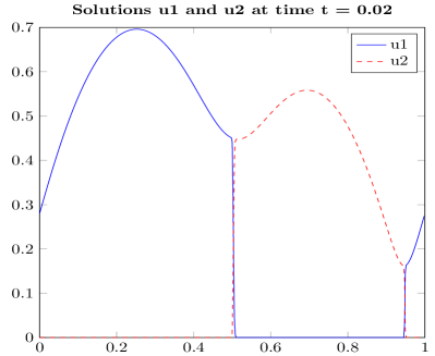
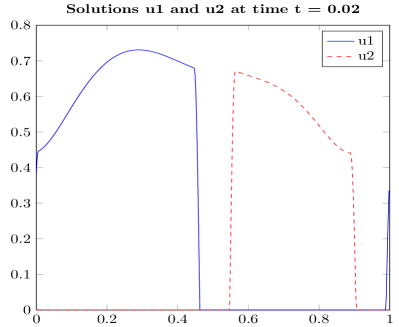
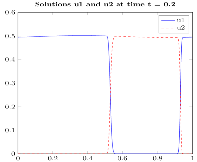
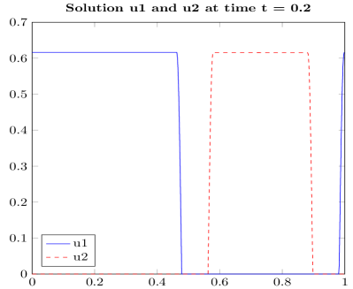
Figure 1. Comparison of the segregation pattern for two species at times $t=0.02$ (top) and $t=0.2$ (bottom) obtained from the local model (left) and nonlocal model (right). The solutions are almost in the steady state at $t=0.2$.

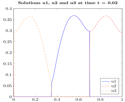
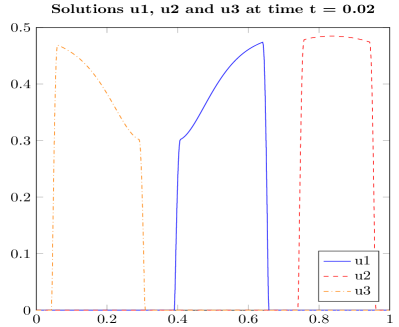
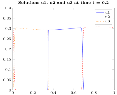
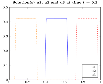
Figure 2. Comparison of the segregation patterns for three species at times $t=0.02$ (top) and $t=0.2$ (bottom) obtained from the local model (left) and nonlocal model (right). The solutions are almost in the steady state at $t=0.2$.

Appendix A Some auxiliary results

Lemma 13.

Under Hypothesis (H3), the entropy dissipation $Q$, defined in (9), is nonnegative.

Proof.

We follow the approach of [12] and write $Q=Q_{1}+\cdots+Q_{3}$, where

$$Q_{1} =\frac{1}{n-1}\sum_{i,j=1,\,i<j}^{n}\int_{\mathbb{T}}\pi_{i}a_{ii}|\partial_{x}u_{i}(x)|^{2}dx+\frac{1}{n-1}\sum_{i,j=1,\,i>j}^{n}\int_{\mathbb{T}}\pi_{i}a_{ii}|\partial_{x}u_{i}(y)|^{2}dy,$$

$$Q_{2} =\sum_{i,j=1,\,i<j}^{n}\int_{\mathbb{T}}\int_{{\mathbb{T}}}\pi_{i}a_{ij}B^{ij}(x-y)\partial_{x}u_{j}(y)\partial_{x}u_{i}(x)dydx,$$

$$Q_{3} =\sum_{i,j=1,\,i>j}^{n}\int_{\mathbb{T}}\int_{{\mathbb{T}}}\pi_{i}a_{ij}B^{ij}(x-y)\partial_{x}u_{j}(y)\partial_{x}u_{i}(x)dydx.$$

Exchanging $i$ and $j$ in the second integral of $Q_{1}$ and using $\operatorname{m}({\mathbb{T}})=1$, we have

$$Q_{1}=\frac{1}{n-1}\sum_{i,j=1,\,i<j}^{n}\int_{\mathbb{T}}\int_{\mathbb{T}}\big{(}\pi_{i}a_{ii}|\partial_{x}u_{i}(x)|^{2}dx+\pi_{j}a_{jj}|\partial_{x}u_{j}(y)|^{2}\big{)}dydx.$$

Exchanging $i$ and $j$ as well as $x$ and $y$ in $Q_{3}$ gives

$$Q_{3} =\sum_{i,j=1,\,i<j}^{n}\int_{\mathbb{T}}\int_{{\mathbb{T}}}\pi_{j}a_{ji}B^{ji}(y-x)\partial_{x}u_{j}(y)\partial_{x}u_{i}(x)dydx$$

$$=\sum_{i,j=1,\,i<j}^{n}\int_{\mathbb{T}}\int_{{\mathbb{T}}}\pi_{j}a_{ji}B^{ij}(x-y)\partial_{x}u_{j}(y)\partial_{x}u_{i}(x)dydx.$$

We collect these expressions to obtain

$$Q=\frac{1}{(n-1)}\sum_{i,j=1,\,i<j}^{n}\int_{\mathbb{T}}\int_{\mathbb{T}}\begin{pmatrix}\partial_{x}u_{i}(x)\\ \partial_{x}u_{j}(y)\end{pmatrix}^{\top}M^{ij}(x-y)\begin{pmatrix}\partial_{x}u_{i}(x)\\ \partial_{x}u_{j}(y)\end{pmatrix}dydx\geq 0,$$

where $M^{ij}$ is defined in (8), and the last inequality follows from Hypothesis (H3). ∎

Lemma 14.

The upwind approximation (15) and the logarithmic mean (16) satisfy property (14) of the mobilities $u_{i,\sigma}$.

Proof.

The proof is based on the following inequalities for the logarithmic mean:

(48) $$\min\{a,b\}\leq\frac{a-b}{\log a-\log b}\leq\max\{a,b\}\quad\mbox{for all }a,b>0.$$

They imply the linear growth $u_{i,\ell+1/2}\leq\max\{u_{i,\ell},u_{i,\ell+1}\}$ for the logarithmic mean, which also holds, by definition, for the upwind approximation. We show that property (14) is satisfied for the upwind approximation (15). Let $p_{i,\ell+1}-p_{i,\ell}\geq 0$. Then, by (48),

$$u_{i,\ell+1/2}(p_{i,\ell+1}-p_{i,\ell})(\log u_{i,\ell+1}-\log u_{i,\ell}) =u_{i,\ell+1}(p_{i,\ell+1}-p_{i,\ell})(\log u_{i,\ell+1}-\log u_{i,\ell})$$

$$\geq(p_{i,\ell+1}-p_{i,\ell})(u_{i,\ell+1}-u_{i,\ell}).$$

On the other hand, if $p_{i,\ell+1}-p_{i,\ell}<0$, again by (48),

$$u_{i,\ell+1/2}(p_{i,\ell+1}-p_{i,\ell})(\log u_{i,\ell+1}-\log u_{i,\ell}) =u_{i,\ell}(p_{i,\ell+1}-p_{i,\ell})(\log u_{i,\ell+1}-\log u_{i,\ell})$$

$$\geq(p_{i,\ell+1}-p_{i,\ell})(u_{i,\ell+1}-u_{i,\ell}).$$

Property (14) follows immediately after inserting definition (16) of the logarithmic mean. This ends the proof. ∎

Lemma 15 (Discrete Young convolution inequality).

Let $1\leq p,q\leq\infty$ and $1\leq r\leq\infty$ be such that $1+1/r=1/p+1/q$ and let $B\in L^{p}({\mathbb{T}})$ and $v=(v_{\ell})_{\ell\in G}\in\mathcal{V}_{\mathcal{T}}$. Furthermore, let $B_{\ell-\ell^{\prime}}=(\Delta x)^{-1}\int_{K_{\ell-\ell^{\prime}}}B(y)dy$ for every $\ell$ and $\ell^{\prime}\in G$. Then

$$\bigg{(}\sum_{\ell\in G}\Delta x\bigg{|}\sum_{\ell^{\prime}\in G}\Delta xB_{\ell-\ell^{\prime}}\,v_{\ell^{\prime}}\bigg{|}^{r}\bigg{)}^{1/r}\leq\|B\|_{L^{p}({\mathbb{T}})}\|v\|_{0,q,{\mathcal{T}}}.$$

Proof.

First, let $\ell\in G$ be fixed. Then

$$\bigg{|}\sum_{\ell^{\prime}\in G}\Delta xB_{\ell-\ell^{\prime}}v_{\ell^{\prime}}\bigg{|}\leq\sum_{\ell^{\prime}\in G}\Delta x\big{(}|B_{\ell-\ell^{\prime}}|^{p}|v_{\ell^{\prime}}|^{q}\big{)}^{1/r}|B_{\ell-\ell^{\prime}}|^{(r-p)/r}|v_{\ell^{\prime}}|^{(r-q)/r}.$$

Thanks to the assumption $1=1/p+1/q-1/r$, we can apply Hölder’s inequality with exponents $r$, $pr/(r-p)$, and $qr/(r-q)$ to obtain

$$\bigg{|}\sum_{\ell^{\prime}\in G}\Delta xB_{\ell-\ell^{\prime}}v_{\ell^{\prime}}\bigg{|} \leq\bigg{(}\sum_{\ell^{\prime}\in G}\Delta x|B_{\ell-\ell^{\prime}}|^{p}|v_{\ell^{\prime}}|^{q}\bigg{)}^{1/r}\bigg{(}\sum_{\ell^{\prime}\in G}\Delta x|B_{\ell-\ell^{\prime}}|^{p}\bigg{)}^{(r-p)/pr}$$

$$\phantom{xx}{}\times\bigg{(}\sum_{\ell^{\prime}\in G}\Delta x|v_{\ell^{\prime}}|^{q}\bigg{)}^{(r-q)/qr}$$

$$=\bigg{(}\sum_{\ell^{\prime}\in G}\Delta x|B_{\ell-\ell^{\prime}}|^{p}|v_{\ell^{\prime}}|^{q}\bigg{)}^{1/r}\|B\|^{(r-p)/r}_{0,p,{\mathcal{T}}}\|v\|^{(r-q)/r}_{0,q,{\mathcal{T}}}.$$

Then, taking the exponent $r$ and summing over $\ell\in G$,

$$\sum_{\ell\in G}\Delta x\bigg{|}\sum_{\ell^{\prime}\in G}\Delta xB_{\ell-\ell^{\prime}}v_{\ell^{\prime}}\bigg{|}^{r} \leq\|B\|^{r-p}_{0,p,{\mathcal{T}}}\|v\|^{r-q}_{0,q,{\mathcal{T}}}\bigg{(}\sum_{\ell\in G}\Delta x\sum_{\ell^{\prime}\in G}\Delta x|B_{\ell-\ell^{\prime}}|^{p}|v_{\ell^{\prime}}|^{q}\bigg{)}$$

$$\leq\|B\|^{r-p}_{0,p,{\mathcal{T}}}\|v\|^{r-q}_{0,q,{\mathcal{T}}}\bigg{(}\sum_{\ell^{\prime}\in G}\Delta x|v_{\ell^{\prime}}|^{q}\sum_{\ell\in G}\Delta x|B_{\ell-\ell^{\prime}}|^{p}\bigg{)}$$

$$\leq\|B\|^{r-p}_{0,p,{\mathcal{T}}}\|v\|^{r-q}_{0,q,{\mathcal{T}}}\|v\|^{q}_{0,q,{\mathcal{T}}}\|B\|^{p}_{0,p,{\mathcal{T}}}=\|B\|^{r}_{0,p,{\mathcal{T}}}\|v\|^{r}_{0,q,{\mathcal{T}}}.$$

Finally, it holds that

$$\|B\|^{p}_{0,p,{\mathcal{T}}} \leq\sum_{\ell\in G}\Delta x\bigg{|}\frac{1}{\Delta x}\int_{K_{\ell}}B(y)dy\bigg{|}^{p}\leq\sum_{\ell\in G}\bigg{(}\int_{K_{\ell}}|B(y)|^{p}dy\bigg{)}\bigg{(}\int_{K_{\ell}}\frac{dx}{\Delta x}\bigg{)}^{p-1}$$

$$\leq\sum_{\ell\in G}\int_{K_{\ell}}|B(y)|^{p}dy=\|B\|^{p}_{L^{p}({\mathbb{T}})},$$

which concludes the proof. ∎

Lemma 16.

Let $s>1$ and $p>1$. Then for any sequence $u=(u_{\ell})_{\ell\in G}$, there exists a constant $C>0$ only depending on $s$ such that

$$\|u\|_{0,\infty,{\mathcal{T}}}\leq C\|u\|_{1,p,{\mathcal{T}}}^{1/s}\|u\|^{1-1/s}_{0,(s-1)p/(p-1),{\mathcal{T}}}.$$

Proof.

We adapt the proof of [5, Lemma 4.1] to the one-dimensional case. By the embedding $\mathrm{BV}({\mathbb{T}})\hookrightarrow L^{\infty}({\mathbb{T}})$ applied to the sequence $(|u_{\ell}|^{s})_{\ell\in G}$,

(49) $$\|u\|_{0,\infty,{\mathcal{T}}}^{s}\leq C\bigg{(}\|u\|^{s}_{0,s,{\mathcal{T}}}+\sum_{\ell\in G}\big{|}|u_{\ell}|^{s}-|u_{\ell+1}|^{s}\big{|}\bigg{)}.$$

Since $s>1$, we have

$$\sum_{\ell\in G}\big{|}|u_{\ell}|^{s}-|u_{\ell+1}|^{s}\big{|}\leq s\sum_{\ell\in G}\big{(}|u_{\ell}|^{s-1}+|u_{\ell+1}|^{s-1}\big{)}|u_{\ell}-u_{\ell+1}|.$$

We apply Hölder’s inequality with exponents $p$ and $p/(p-1)$:

$$\sum_{\ell\in G}\big{|}|u_{\ell}|^{s}-|u_{\ell+1}|^{s}\big{|}\leq 2s\bigg{(}\sum_{\ell\in G}\frac{|u_{\ell}-u_{\ell+1}|^{p}}{\Delta x^{p-1}}\bigg{)}^{1/p}\bigg{(}\sum_{\ell\in G}\Delta x|u_{\ell}|^{\frac{(s-1)p}{p-1}}\bigg{)}^{(p-1)/p}.$$

Besides, using again Hölder’s inequality (with the same exponents), we find that

$$\|u\|_{0,s,{\mathcal{T}}}=\bigg{(}\sum_{\ell\in G}\Delta x|u_{\ell}||u_{\ell}|^{s-1}\bigg{)}^{1/s}\leq\|u\|^{1/s}_{0,p,{\mathcal{T}}_{m}}\|u\|^{(s-1)/s}_{0,(s-1)p/(p-1),{\mathcal{T}}}.$$

Then, inserting the last two inequalities into (49) yields the desired result. This concludes the proof of Lemma 16. ∎

Appendix B Counter-example

We claim that there exist kernels $B^{ij}$, being an indicator function, and piecewise constant functions $u_{1},\ldots,u_{n}$ such that the positive semi-definiteness condition

$$J:=\sum_{i,j=1}^{n}\int_{\mathbb{T}}\int_{\mathbb{T}}\pi_{i}a_{ij}B^{ij}(x-y)u_{j}(y)u_{i}(x)dydx\geq 0$$

is not satisfied. For this statement, we assume that the matrix $(\pi_{i}a_{ij})\in{\mathbb{R}}^{n\times n}$ is (symmetric and) positive definite. With the notation of Section 2.1, we set $\Delta x=1/N$ for some even number $N>5$ and choose $r=3\Delta x/2$ as well as the kernels

$$B^{ij}(x)=\mathrm{1}_{(-r,r)}(x)\quad\mbox{for }x\in{\mathbb{T}}.$$

Let $u_{i}=(u_{i,\ell})_{\ell\in G}\in\mathcal{V}_{\mathcal{T}}$ for $i=1,\ldots,n$. Then we can write $J$ as

(50) $$J=\sum_{i,j=1}^{n}\sum_{\ell,\ell^{\prime}\in G}\pi_{i}a_{ij}\widehat{M}^{ij}_{\ell,\ell^{\prime}}u_{j,\ell^{\prime}}u_{i,\ell},\quad\mbox{where }\widehat{M}^{ij}_{\ell,\ell^{\prime}}=\int_{K_{\ell}}\int_{K_{\ell^{\prime}}}B^{ij}(x-y)dydx.$$

A straightforward, but rather tedious computation shows that the matrix $\widehat{M}^{ij}=(\widehat{M}^{ij}_{\ell,\ell^{\prime}})_{\ell,\ell^{\prime}\in G}$ $\in{\mathbb{R}}^{N\times N}$ is pentadiagonal with entries

$$M_{\ell,\ell^{\prime}}^{ij}=(\Delta x)^{2},\quad M_{\ell,\ell\pm 1}^{ij}=\frac{7}{8}(\Delta x)^{2},\quad M_{\ell,\ell\pm 2}^{ij}=\frac{1}{8}(\Delta x)^{2}.$$

This matrix possesses the eigenvector $w\in{\mathbb{R}}^{N}$, defined by $w_{\ell}=1$ for $\ell$ odd and $w_{\ell}=-1$ for $\ell$ even, associated with the negative eigenvalue $\lambda=-4(\Delta x)^{2}$.

Let $v_{1},\ldots,v_{n}\in{\mathbb{R}}^{n}$ be the eigenvectors of the symmetric matrix $(\pi_{i}a_{ij})_{i,j=1,\ldots,n}$ associated with the eigenvalues $0<\nu_{1}\leq\ldots\leq\nu_{n}$, respectively. We define the $nN\times nN$ matrix $\widehat{M}=(\pi_{i}a_{ij}\widehat{M}^{ij})$ consisting of the $N\times N$ blocks $\pi_{i}a_{ij}\widehat{M}^{ij}$. It can be verified that the matrix $\widehat{M}$ possesses the eigenvector $z=(z_{1},\ldots,z_{n})\in{\mathbb{R}}^{nN}$ with $z_{i}=v_{n,i}w\in{\mathbb{R}}^{N}$ for $i=1,\ldots,n$ associated with the eigenvalue $\lambda\nu_{n}=-4(\Delta x)^{2}\nu_{n}$. Then, choosing $u_{i}=z_{i}$ in (50), we find that

$$J=\sum_{i,j=1}^{n}\pi_{i}a_{ij}z_{i}^{\top}\widehat{M}^{ij}z_{j}=-4(\Delta x)^{2}\nu_{n}\sum_{i=1}^{n}|z_{i}|^{2}<0.$$

This provides the desired counter-example.

References

- [1] V. Anaya, M. Bendahmane, and M. Sepúlveda. Numerical analysis for a three interacting species model with nonlocal and cross diffusion. ESAIM: Math. Model. Numer. Anal. 49 (2015), 171–192.
- [2] N. Ayi, M. Herda, H. Hivert, and I. Tristani. On a structure-preserving numerical method for fractional Fokker–Planck equations. Math. Comp. 92 (2023), 635–693.
- [3] M. Bendahmane and M. Sepúlveda. Convergence of a finite volume scheme for nonlocal reaction-diffusion systems modelling an epidemic disease. Discrete Cont. Dyn. Sys. B 11 (2009), 823–853.
- [4] M. Bertsch, M.E. Gurtin, D. Hilhorst and L.A. Peletier. On interacting populations that disperse to avoid crowding: preservation of segregation. J. Math. Biol. 23 (1985), 1–13.
- [5] M. Bessemoulin-Chatard, C. Chainais-Hillairet, and F. Filbet. On discrete functional inequalities for some finite volume schemes. IMA J. Numer. Anal. 35 (2015), 1125–1149.
- [6] J. A. Carrillo, A. Chertock, and Y. Huang. A finite-volume method for nonlinear nonlocal equations with a gradient flow structure. Commmun. Comput. Phys. 17 (2015), 233–258.
- [7] J. A. Carrillo, F. Filbet, and M. Schmidtchen. Convergence of a finite volume scheme for a system of interacting species with cross-diffusion. Numer. Math. 145 (2020), 473–511.
- [8] J. A. Carrillo, Y. Huang, and M. Schmidtchen. Zoology of a nonlocal cross-diffusion model for two species. SIAM J. Appl. Math. 78 (2018), 1078–1104.
- [9] C. Chainais-Hillairet, J.-G. Liu, and Y.-J. Peng. Finite volume scheme for multi-dimensional drift-diffusion equations and convergence analysis. ESAIM Math. Model. Numer. Anal. 37 (2003), 319–338.
- [10] L. Chen, E. Daus, and A. Jüngel. Rigorous mean-field limit and cross diffusion. Z. Angew. Math. Phys. 70 (2019), no. 122, 21 pages.
- [11] K. Deimling. Nonlinear Functional Analysis. Springer, Berlin, 1985.
- [12] H. Dietert and A. Moussa. Persisting entropy structure for nonlocal cross-diffusion systems. To appear in Ann. Fac. Sci. Toulouse, 2023. arXiv:2101.02893.
- [13] R. Eymard, T. Gallouët, and R. Herbin. Finite Volume Methods. In: P. G. Ciarlet and J.-L. Lions (eds.), Handbook of Numerical Analysis 7 (2000), 713–1018.
- [14] T. Gallouët, J.-C. Latché. Compactness of discrete approximate solutions to parabolic PDEs – Application to a turbulence model. Commun. Pure Appl. Anal. 11 (2012), 2371–2391.
- [15] M. Herda and A. Zurek. Study of a structure preserving finite volume scheme for a nonlocal cross-diffusion system. Submitted for publication, 2022. hal-03714164v2.
- [16] A. Jüngel, S. Portisch, A. Zurek. Nonlocal cross-diffusion systems for multi-species populations and networks. Nonlin. Anal. 219 (2022), no. 112800, 26 pages.
- [17] A. Jüngel and A. Zurek. A convergent structure-preserving finite-volume scheme for the Shigesada–Kawasaki–Teramoto population system. SIAM J. Numer. Anal. 59 (2021), 2286–2309.
- [18] G. Galiano. Error analysis of some nonlocal diffusion discretization schemes. Comput. Math. Appl. 103 (2021), 40–52.
- [19] G. Medvedev and G. Simpson. A numerical method for a nonlocal diffusion equation with additive noise. Stoch. PDE: Anal. Comput., in press, 2023.
- [20] J. R. Potts and M. A. Lewis. Spatial memory and taxis-driven pattern formation in model ecosystems. Bull. Math. Biol. 81 (2019), 2725–2747.
- [21] C. Rao. Diversity and dissimilarity coefficients: a unified approach. Theor. Popul. Biol. 21 (1982), 24–43.
- [22] F. Santambrogio. Optimal transport for applied mathematicians. Calculus of variations, PDEs, and modeling. Prog. Nonlinear Differ. Equ. Appl., Cham: Birkhäuser/Springer, 2015.